Wireless Information and Power Transfer in Relay Systems with Multiple Antennas and Interference

Abstract

In this paper, an energy harvesting dual-hop relaying system without/with the presence of co-channel interference (CCI) is investigated. Specifically, the energy constrained mutli-antenna relay node is powered by either the information signal of the source or via the signal receiving from both the source and interferer. In particular, we first study the outage probability and ergodic capacity of an interference free system, and then extend the analysis to an interfering environment. To exploit the benefit of multiple antennas, three different linear processing schemes are investigated, namely, 1) Maximum ratio combining/maximal ratio transmission (MRC/MRT), 2) Zero-forcing/MRT (ZF/MRT) and 3) Minimum mean-square error/MRT (MMSE/MRT). For all schemes, both the system s outage probability and ergodic capacity are studied, and the achievable diversity order is also presented. In addition, the optimal power splitting ratio minimizing the outage probability is characterized. Our results show that the implementation of multiple antennas increases the energy harvesting capability, hence, significantly improves the system s performance. Moreover, it is demonstrated that the CCI could be potentially exploited to substantially boost the performance, while the choice of a linear processing scheme plays a critical role in determining how much gain could be extracted from the CCI.

I Introduction

Energy harvesting technique, as an emerging solution for prolonging the lifetime of the energy constrained wireless devices, has gained significant interests in recent years. The conventional energy harvesting techniques rely on the external natural resources, such as solar power, wind energy or thermoelectric effects [1, 2, 3]. However, due to the randomness and intermittent property of external natural resources, communication systems employing the conventional energy harvesting technique can not guarantee the delivery of reliable and uninterrupted communication services. Recently, the wireless energy transfer technique, first demonstrated by Nikola Tesla, has rekindled its interest in the context of energy harvesting communication systems where radio-frequency (RF) signals are used as an energy source [4, 5, 6, 7, 8]. Since RF signals can be under control, it is much more reliable than external natural resources, hence, wireless energy harvesting using RF signals is a promising technique to power communication devices [9].

Since RF signals are capable of carrying both the information and energy, a new research area, namely simultaneous wireless information and power transfer (SWIPT), has recently emerged. The seminal works [6, 7] have characterized the fundamental tradeoff between the harvested energy and information capacity. Nevertheless, it was assumed in [6] that the receiver can decode the information and harvest energy from the same signal simultaneously, which is unfortunately impossible due to practical circuit limitations. To this end, the work in [10] proposed two practical receiver architectures, namely, “time-switching”, where the receiver switches between decoding information and harvesting energy, and “power-splitting”, where the receiver splits the signal into two streams, one for information decoding and the other for energy harvesting. Since then, a number of works have appeared in the literature investigating different aspects of simultaneous information and energy transfer with practical receivers [11, 12]. Specifically, in [11], an opportunistic RF energy harvesting scheme for single-input-single-output systems with co-channel interference (CCI) was investigated, where it was shown that the CCI can be identified as a potential energy source. Later on, an improved receiver, i.e., the dynamic power splitting receiver was studied in [12]. The extension of [10] to the scenario with imperfect channel state information (CSI) at the transmitter was studied in [13]. For multiple-input single-output (MISO) channels, the optimal beamforming designs for SWIPT systems with/without secrecy constraint have been investigated in [14, 15], and the optimal transmission strategy maximizing the system throughput of MISO interference channel has been studied in [16]. Moreover, the application of RF energy transfer technique in cognitive radio networks with multiple antennas at the secondary transmitter was considered in [17]. Finally, cellular networks with RF energy transfer were considered in [8, 18]. It is worth noting that all these prior works focus on the point-to-point communication systems.

The RF energy harvesting technique also finds important applications in cooperative relaying networks, where an energy-constrained relay with limited battery reserves relies on some external charging mechanism to assist the transmission of source information to the destination [2]. As such, a number of works have exploited the idea of achieving simultaneous information and energy transfer in cooperative relaying systems [19, 20, 21, 4, 9]. Specifically, [20] studied the throughput performance of an amplify-and-forward (AF) relaying system for both time-switching and power-splitting protocols and [21] considered the power allocation strategies for decode-and-forward (DF) relaying system with multiple source-destination pairs. More recently, the performance of energy harvesting cooperative networks with randomly distributed users was studied in [4, 9]. However, all these works are limited to the single antenna setup and all assume an interference free environment.

Motivated by this, we consider a dual-hop AF relaying system where the source and destination are equipped with a single antenna while the relay is equipped with multiple antennas. The energy constrained relay collects energy from ambient RF signals and uses the harvested energy to forward the information to the destination node. The power-splitting receiver architecture proposed in [10] is adopted. Specifically, we first study the performance of the multiple antenna relay system without CCI, which serves as a benchmark for the performance in the presence of CCI. Then, we present a detailed performance analysis for the system assuming a single dominant interferer at the relay. It is worth pointing out that, in the energy harvesting relaying system, while CCI provides additional energy, it corrupts the desired signal. In order to exploit CCI as a beneficial prospect, three different linear processing schemes, namely, 1) Maximum ratio combining/maximal ratio transmission (MRC/MRT), 2) Zero-forcing/MRT (ZF/MRT), 3) Minimum mean-square error/MRT (MMSE/MRT) are investigated.

The main contributions of this paper are summarized as follows:

• For the scenario without CCI, we derive an exact outage expression involving a single integral, and a tight closed-form outage probability lower bound. In addition, we present a simple high signal-to-noise ratio (SNR) approximation, which reveals that the system achieves a diversity order of $N$, where $N$ is the number of relay antennas. A new tight closed-form upper bound for the ergodic capacity is also derived. Finally, the optimal power splitting ratio minimizing the outage probability is characterized.

• For the scenario with CCI, we present tight closed-form outage probability lower bounds and capacity upper bounds for all three schemes. In addition, we also characterize the high SNR outage behavior and show that both the MRC/MRT and MMSE/MRT schemes achieve a diversity order of $N$, while the ZF/MRT only achieves a diversity order of $N-1$. Moreover, the optimal power splitting ratio minimizing the outage probability is studied.

• The presented analytical expressions provide an efficient means to evaluate key system performance metrics, such as the outage probability and ergodic capacity, without resorting to time-consuming Monte Carlo simulations. Therefore, a fast assessment of the impact of various key system parameters such as the energy harvesting efficiency $\eta$, the number of antennas $N$, the source transmitting power $\rho_{1}$ and the interference power $\rho_{I}$ on the optimal power splitting ratio is enabled.

• Our results demonstrate that the CCI could be potentially exploited to significantly improve the system’s performance. However, the actual performance gain due to CCI depends heavily on the choice of linear processing schemes. It is shown that the MMSE/MRT scheme is always capable of turning the CCI as a desired factor, and can achieve higher performance gain when the CCI is strong. On the other hand, CCI is not always beneficial when the MRC/MRT and ZF/MRT schemes are used. The performance degrades significantly in the strong CCI scenario if the MRC/MRT scheme is applied. In contrast, a weak interferer degrades the performance of the ZF/MRT scheme, which on the other hand achieves almost the same performance as the MMSE/MRT scheme in the presence of strong CCI.

The remainder of the paper is organized as follows: Section II introduces the system model. Section III investigates of the performance of the system without CCI. Section IV addresses the scenario with CCI. Numerical results and discussions are provided in Section V. Finally, Section VI concludes the paper and summarizes the key findings.

Notation: We use bold upper case letters to denote matrices, bold lower case letters to denote vectors and lower case letters to denote scalars. ${\left\|{\bf{h}}\right\|_{F}}$ denotes the Frobenius norm; ${\tt E}\{x\}$ stands for the expectation of the random variable $x$; ${*}$ denotes the conjugate operator, while $T$ denotes the transpose operator and ${{\dagger}}$ denotes the conjugate transpose operator; ${{\cal CN}(0,1)}$ denotes a scalar complex Gaussian distribution with zero mean and unit variance; $\Gamma(x)$ is the gamma function; $\Psi\left({a,b;z}\right)$ is the confluent hypergeometric function [24, Eq. (9.210.2)]; $K_{v}(x)$ is the $v$-th order modified Bessel function of the second kind [24, Eq. (8.407.1)]; ${\rm Ei}(x)$ is the exponential integral function [24, Eq. (8.211.1)]; $\Gamma\left({\alpha,x}\right)$ is the upper incomplete gamma function [24, Eq. (8.350.2)]; ${}_{2}{F_{1}}(a,b;c;z)$ is the Gauss Hypergeometric function [24, Eq. (9.100)]; $\psi\left(x\right)$ is the Digamma function [24, Eq. (8.360.1)]; ${\mathop{\rm G}\nolimits}_{p,q}^{m,n}\left(\cdot\right)$ is the Meijer G-function [24, Eq. (9.301)] and ${\mathop{\rm G}\nolimits}_{1,[1:1],0,[1:1]}^{1,1,1,1,1}\left(\cdot\right)$ denotes the generalized Meijer G-function of two variables [25] which can be computed by the algorithm presented in [26, Table II].

II System Model

We consider a dual-hop multiple antenna AF energy harvesting relaying system as shown in Fig. 1, where both the source and the destination are equipped with a single antenna, while the relay is equipped with $N$ antennas [5]. The source sends information to the destination through an energy constrained relay node. Throughout this paper, the following assumptions are adopted: 1) It is assumed that direct link between the source and the destination does not exist due to obstacles and/or severe fading. 2) The channel remains constant over the block time $T$ and varies independently and identically from one block to the other, and has a Rayleigh distributed magnitude. 3) As in [27, 28, 29], no CSI is assumed at the source, full CSI is assumed at the relay, and local CSI is assumed at the destination.

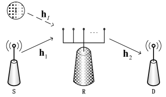
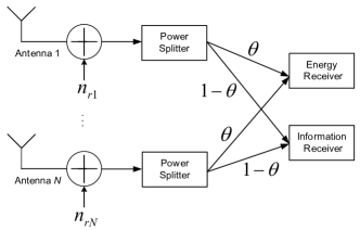
Figure 1: (a) System model: S, R and D denote the source, relay and destination node, respectively. (b) Block diagram of the relay receiver with the power splitting protocol.

We focus on the power splitting protocol proposed in [10]. Specifically, the entire communication consists of two time slots with duration of $\frac{T}{2}$ each. At the end of the first phase, each antenna at the relay node splits the received source signal into two streams, one for energy harvesting and the other for information processing as depicted in Fig. 1. As in [21, 12], we consider the pessimistic case where power splitting only reduces the signal power, but not the noise power. Hence, our results provide a lower bound on the performance for practical systems. We now consider two separate cases depending on whether the relay is subject to CCI or not.

II-A Noise-limited Case

Let $\theta$ denote the power splitting ratio, then the signal component at the input of the information receiver is given by

$${{\bf{y}}_{r}}=\sqrt{{(1-\theta){P_{s}}}/{d_{1}^{\tau}}}{{\bf{h}}_{1}}x+{{\bf{n}}_{r}},$$ (1)

where $P_{s}$ denotes the source power, ${{{\bf h}}_{{1}}}$ is an ${N\times 1}$ vector with entries following identically and independently distributed (i.i.d.) ${{\cal CN}(0,1)}$, $d_{1}$ denotes the distance between the source and the relay, $\tau$ is the path loss exponent, $x$ is the source message with unit power, ${{{\bf n}}_{{r}}}$ is an ${N\times 1}$ vector and denotes the additive white Gaussian noise (AWGN) with ${\tt E}\{\mathbf{n}_{r}\mathbf{n}_{r}^{{\dagger}}\}=N_{0}{\mathbf{I}}$.

At the end of the first phase, the overall energy harvested during half of the block time $\frac{T}{2}$, can be expressed as

$${E_{h}}=\frac{\eta\theta{P_{s}}}{d_{1}^{\tau}}\left\|{{{\bf{h}}_{1}}}\right\|_{F}^{2}\frac{T}{2},$$ (2)

where $\eta$ denotes the RF-to-DC conversion efficiency.

II-B Interference plus Noise Case

We assume that the relay is subjected to a single dominant interferer and AWGN while the destination is still corrupted by the AWGN only. It is worth pointing out the single dominant interferer assumption has been widely adopt in the literature, see [31, 32] and references therein. Moreover, such a system model enables us to gain key insights on the joint effect of CCI and multiple antennas in an energy harvesting relaying system.

In such case, the signal at the input of the information receiver at the relay is given by

$${{\bf{y}}_{r}}=\sqrt{{(1-\theta){P_{s}}}/{d_{1}^{\tau}}}{{\bf{h}}_{1}}x+\sqrt{{(1-\theta){P_{I}}}/{{d_{I}^{\tau}}}}{{\bf{h}}_{I}}{s_{I}}+{{\bf{n}}_{r}},$$ (3)

where $P_{I}$ is the interference power, $d_{I}$ denotes the distance between the interferer and the relay, ${s_{I}}$ is the interference symbol with unit power, and ${{{\bf h}}_{{I}}}$ is an ${N\times 1}$ vector with entries following i.i.d. ${{\cal CN}(0,1)}$.

Also, according to [11], at the end of the first phase, the overall energy harvested during half of the block time $\frac{T}{2}$ is given by

$${E_{h}}=\eta\theta\left({\frac{P_{s}}{d_{1}^{\tau}}\left\|{{{\bf{h}}_{1}}}\right\|_{F}^{2}+\frac{P_{I}}{d_{I}^{\tau}}\left\|{{{\bf{h}}_{I}}}\right\|_{F}^{2}}\right)\frac{T}{2}.$$ (4)

For both cases, during the second phase, the relay transmits a transformed version of the received signal to the destination using the harvested power. Hence, the signal at the destination can be expressed as

$${y_{d}}=\sqrt{{1}/{d_{2}^{\tau}}}{{\bf{h}}_{2}}{\bf{W}}{{\bf{y}}_{r}}+{n_{d}},$$ (5)

where ${{\bf{h}}_{{2}}}$ is a ${1\times N}$ vector and denotes the relay-destination channel and its entries follow i.i.d. ${{\cal CN}(0,1)}$, $d_{2}$ denotes the distance between the relay and the destination, ${n_{d}}$ is the AWGN at the destination with ${\tt E}\{n_{d}^{*}n_{d}\}=N_{0}$, $\mathbf{W}$ is the transformation matrix applied at the information receiver at the relay with ${\tt E}\{\left\|\mathbf{W}\mathbf{y}_{r}\right\|_{F}^{2}\}=P_{r}$. Obviously, the performance of the system depends on the choice of $\mathbf{W}$, which will be elaborated in the ensuing sections.

III The noise-limited Scenario

In this section, we consider the scenario where the relay is corrupted by AWGN only. In such case, it can be shown that the optimal transformation matrix $\bf{W}$ has the following structure:

$${\bf{W}}=\omega\frac{{{\bf{h}}_{2}^{\bf{{\dagger}}}}{{\bf{h}}_{1}^{\bf{{\dagger}}}}}{{\left\|{{{\bf{h}}_{2}}}\right\|}_{F}{\left\|{{{\bf{h}}_{1}}}\right\|}_{F}},$$ (6)

where $\omega$ is the power constraint factor, i.e., the information receiver first applies the MRC principle to combine all the signals from $N$ antennas, and then forward the signal to the destination by using the MRT principle. To guarantee the transmit power constraint at the relay, $\omega$ can be computed as

$${\omega^{2}}=\frac{{P_{r}}}{{\frac{\left({1-\theta}\right){P_{s}}}{d_{1}^{\tau}}\left\|{{{\bf{h}}_{1}}}\right\|_{F}^{2}+{N_{0}}}},$$ (7)

where $P_{r}$ is the available relay power. Since the relay communicates with the destination for half of the block time $\frac{T}{2}$, we have ${P_{r}}=\frac{{{E_{h}}}}{{{T\mathord{\left/{\vphantom{T2}}\right.\kern-1.2pt}2}}}=\frac{\eta\theta{P_{s}}}{d_{1}^{\tau}}\left\|{{{\bf{h}}_{1}}}\right\|_{F}^{2}.$ Hence, the end-to-end SNR of the system can be expressed as

$$\gamma =\frac{{{\omega^{2}}\left\|{{{\bf{h}}_{2}}}\right\|_{F}^{2}\left\|{{{\bf{h}}_{1}}}\right\|_{F}^{2}\frac{\left({1-\theta}\right){P_{s}}}{d_{1}^{\tau}d_{2}^{\tau}}}}{{{\omega^{2}}\left\|{{{\bf{h}}_{2}}}\right\|_{F}^{2}\frac{N_{0}}{d_{2}^{\tau}}+{N_{0}}}}$$

$$=\frac{{\frac{\eta\theta\left({1-\theta}\right)\rho_{1}^{2}}{d_{1}^{2\tau}d_{2}^{\tau}}\left\|{{{\bf{h}}_{2}}}\right\|_{F}^{2}\left\|{{{\bf{h}}_{1}}}\right\|_{F}^{4}}}{{\frac{\eta\theta{\rho_{1}}}{{d_{1}^{\tau}d_{2}^{\tau}}}\left\|{{{\bf{h}}_{2}}}\right\|_{F}^{2}\left\|{{{\bf{h}}_{1}}}\right\|_{F}^{2}+\frac{\left({1-\theta}\right){\rho_{1}}}{d_{1}^{\tau}}\left\|{{{\bf{h}}_{1}}}\right\|_{F}^{2}+1}},$$ (8)

where $\rho_{1}$ is defined as ${\rho_{1}}={{P_{s}}}/{{{N_{0}}}}$.

In the following, we give a detailed performance analysis in terms of the outage probability and ergodic capacity. In addition, the optimal $\theta$ minimizing the outage probability is investigated.

III-A Outage Probability

The outage probability is an important performance metric, which is defined as the instantaneous SNR falls below a pre-defined threshold $\gamma_{\sf th}$. Mathematically, outage probability can be expressed as

$${P_{\sf out}}={\mathop{\rm Prob}\nolimits}\left({\gamma<{\gamma_{\sf th}}}\right).$$ (9)

Theorem 1

The outage probability of the multiple antenna energy harvesting relaying system can be expressed as

$${P_{{\sf{out}}}}=1-\int_{d/c}^{\infty}{\frac{{\Gamma\left({N,\frac{{ax+b}}{{c{x^{2}}-dx}}}\right)}}{{\Gamma\left(N\right)}}\frac{{{x^{N-1}}}}{{\Gamma\left(N\right)}}{e^{-x}}dx},$$ (10)

where $a=\frac{\left({1-\theta}\right){\rho_{1}}{\gamma_{{\sf{th}}}}}{d_{1}^{\tau}}$, $b={\gamma_{{\sf{th}}}}$, $c=\frac{\eta\theta\left({1-\theta}\right)\rho_{1}^{2}}{d_{1}^{2\tau}d_{2}^{\tau}}$, $d=\frac{\eta\theta{\rho_{1}}{\gamma_{{\sf{th}}}}}{d_{1}^{\tau}d_{2}^{\tau}}$.

Proof: Substituting (III) into (9), the outage probability of the system can be expressed as

$${P_{{\rm{out}}}}=$$ (11)

$${\rm{Prob}}\left({\left\|{{{\bf{h}}_{2}}}\right\|_{F}^{2}\left({c\left\|{{{\bf{h}}_{1}}}\right\|_{F}^{4}-d\left\|{{{\bf{h}}_{1}}}\right\|_{F}^{2}}\right)<\left({a\left\|{{{\bf{h}}_{1}}}\right\|_{F}^{2}+b}\right)}\right),$$

which can be evaluated as

$${P_{{\rm{out}}}}=\int_{0}^{d/c}{{f_{\left\|{{{\bf{h}}_{1}}}\right\|_{F}^{2}}}\left(x\right)dx}\\ +\int_{d/c}^{\infty}{{f_{\left\|{{{\bf{h}}_{1}}}\right\|_{F}^{2}}}\left(x\right){F_{\left\|{{{\bf{h}}_{2}}}\right\|_{F}^{2}}}\left({\frac{{ax+b}}{{c{x^{2}}-dx}}}\right)dx}.$$ (12)

Since the squared Frobenius norm of a complex Gaussian vector is Chi-square distributed, $\left\|{{{\bf{h}}_{1}}}\right\|_{F}^{2}$ and $\left\|{{{\bf{h}}_{2}}}\right\|_{F}^{2}$ are i.i.d. gamma random variables. After some simple algebraic manipulations (10) is obtained.  $\square$

Theorem 1 presents the exact outage probability of the of the system with arbitrary number of antennas. For the special case with a single antenna at the relay, Theorem 1 reduces to the result derived in [20, Proposition 3]. To the best of the authors’ knowledge, the integral in (10) does not admit a closed-form expression. However, this single integral expression can be efficiently evaluated numerically using software such as Matlab or MATHEMATICA. Alternatively, we can use the following closed-form lower bound for the outage probability, which will be shown to be tight across the entire SNR range in the Section V.

Corollary 1

The outage probability of the multiple antenna energy harvesting relaying system can be lower bounded as

$$P_{{\sf{out}}}^{{\sf{low}}}=1-\frac{{2{e^{-d/c}}}}{{\Gamma\left(N\right)}}\sum\limits_{i=0}^{N-1}{\frac{1}{{i!}}\sum\limits_{j=0}^{N-1}{{N-1}\choose j}}{\left({\frac{d}{c}}\right)^{N-j-1}}\times\\ {\left({\frac{a}{c}}\right)^{\frac{{i+j+1}}{2}}}{K_{i-j-1}}\left({2\sqrt{\frac{a}{c}}}\right).$$ (13)

Proof: See Appendix A.  $\square$

While Theorem 1 and Corollary 1 are useful to study the system’s outage probability, the expressions are in general too complex to gain insight. Motivated by this, we now look into the high SNR regime, and derive a simple approximation for the outage probability, which enables the characterization of the achievable diversity order.

Theorem 2

In the high SNR regime, i.e., ${\rho_{1}}\to\infty$, the outage probability of the multiple antenna energy harvesting relaying system can be approximated as

$$P_{{\sf{out}}}^{\infty}\approx\frac{\left({\frac{{{d_{1}^{\tau}\gamma_{{\sf{th}}}}}}{{{\rho_{1}}}}}\right)^{N}}{{\Gamma\left({N+1}\right)}}\left({\frac{1}{{{{\left({1-\theta}\right)}^{N}}}}}\right.+\\ \left.{\frac{{\ln\left({\left({1-\theta}\right){\rho_{1}}}\right)-\ln{(d_{1}^{\tau}\gamma_{{\sf{th}}})}-{\bf{C}}}}{{\Gamma\left(N\right)}}{{\left({\frac{d_{2}^{\tau}}{{\eta\theta}}}\right)}^{N}}}\right),$$ (14)

where $\bf{C}$ is the Euler-Mascheroni constant [24, Eq. (9.73)].

Proof: See Appendix B.  $\square$

We observe that the system achieves a diversity order of $N$, which is the same as the conventional case with constant power relay node [22]. However, we notice that $P_{\sf out}$ decays as $\rho_{1}^{-N}\ln{\rho_{1}}$ rather than $\rho_{1}^{-N}$ as in the conventional case [22]. This important observation implies that, in the energy harvesting case, the slope of $P_{\sf out}$ converges much slower compared with that in the constant power case. Please note that similar observations have been made in prior work [21]. The possible reason is that, in SWIPT systems, the available transmit power at the relay is a random variable, which results in higher outage probability compared to the conventional constant relay power case.

III-B Ergodic Capacity

Noticing that the end-to-end SNR given in (III) can be alternatively expressed as

$$\gamma=\frac{{{\gamma_{1}}{\gamma_{2}}}}{{{\gamma_{1}}+{\gamma_{2}}+1}},$$ (15)

where ${\gamma_{1}}=\frac{\left({1-\theta}\right){\rho_{1}}}{d_{1}^{\tau}}\left\|{{{\bf{h}}_{1}}}\right\|_{F}^{2}$ and ${\gamma_{2}}=\frac{\eta\theta{\rho_{1}}}{d_{1}^{\tau}d_{2}^{\tau}}\left\|{{{\bf{h}}_{2}}}\right\|_{F}^{2}\left\|{{{\bf{h}}_{1}}}\right\|_{F}^{2}$. The ergodic capacity is given by

$$C=\frac{1}{2}{\mathop{\rm E}\nolimits}\left[{{{\log}_{2}}\left({1+\frac{{{\gamma_{1}}{\gamma_{2}}}}{{{\gamma_{1}}+{\gamma_{2}}+1}}}\right)}\right].$$ (16)

Unfortunately, an exact evaluation of the ergodic capacity is generally intractable, since the cumulative distribution function (c.d.f.) of (III) can not be given in closed-form. Motivated by this, we hereafter seek to deduce a tight bound for the ergodic capacity.

Starting from (16), the ergodic capacity can be alternatively expressed as

$$C=\frac{1}{2}{\mathop{\rm E}\nolimits}\left[{{{\log}_{2}}\left({\frac{{\left({1+{\gamma_{1}}}\right)\left({1+{\gamma_{2}}}\right)}}{{1+{\gamma_{1}}+{\gamma_{2}}}}}\right)}\right]=C_{\gamma_{1}}+C_{\gamma_{2}}-C_{\gamma_{T}},$$ (17)

where $C_{\gamma_{i}}=\frac{1}{2}{\mathop{\rm E}\nolimits}\left[{{{\log}_{2}}\left({1+{\gamma_{i}}}\right)}\right]$, for $i\in\{1,2\}$, and $C_{\gamma_{T}}=\frac{1}{2}{\mathop{\rm E}\nolimits}\left[{{{\log}_{2}}\left({1+{\gamma_{1}}+{\gamma_{2}}}\right)}\right]$. Using the fact that $f\left({x,y}\right)={\log_{2}}\left({1+{e^{x}}+{e^{y}}}\right)$ is a convex function with respect to $x$ and $y$, we have

$${C_{{\gamma_{T}}}}\geq\frac{1}{2}{\log_{2}}\left({1+{e^{{\mathop{\rm E}\nolimits}\left({\ln{\gamma_{1}}}\right)}}+{e^{{\mathop{\rm E}\nolimits}\left({\ln{\gamma_{2}}}\right)}}}\right).$$ (18)

We now establish the ergodic capacity upper bound of the system using the following theorem:

Theorem 3

The ergodic capacity of the multiple antenna energy harvesting relaying system is upper bounded by

$${C_{\sf up}}=\frac{e^{\frac{d_{1}^{\tau}}{{\left({1-\theta}\right){\rho_{1}}}}}}{{2\ln 2}}\sum\limits_{k=0}^{N-1}{{{\left({\frac{d_{1}^{\tau}}{{\left({1-\theta}\right){\rho_{1}}}}}\right)}^{k}}\Gamma\left({-k,\frac{d_{1}^{\tau}}{{\left({1-\theta}\right){\rho_{1}}}}}\right)}+\\ \frac{1}{{2\ln 2}}\frac{1}{{\Gamma\left({\rm{N}}\right)}}\sum\limits_{m=0}^{N-1}\frac{1}{{m!}}{{\left({\frac{d_{1}^{\tau}d_{2}^{\tau}}{{\eta\theta{\rho_{1}}}}}\right)}^{m}}G_{1,3}^{3,1}\left(\frac{d_{1}^{\tau}d_{2}^{\tau}}{{\eta\theta{\rho_{1}}}}\middle|^{-m}_{-m,N-m,0}\right)-\\ \frac{1}{2}{\log_{2}}\left({1+\frac{(1-\theta){\rho_{1}}}{d_{1}^{\tau}}{e^{\psi\left(N\right)}}+\frac{\eta\theta{\rho_{1}}}{d_{1}^{\tau}d_{2}^{\tau}}{e^{2\psi\left(N\right)}}}\right).$$ (19)

Proof: See Appendix C.  $\square$

Theorem 3 presents a new upper bound for the ergodic capacity of the system, which is quite tight across the entire SNR range as shown in the section V, hence, providing an efficient means to evaluate the ergodic capacity without resorting to Monte Carlo simulations. In addition, as we show in the next subsection, it enables the study of the optimal power splitting ratio.

III-C Optimization of the Parameter $\theta$ in High SNR Value

The right selection of the power splitting ratio $\theta$ is crucial for the system’s performance. A high value of $\theta$ could provide more transmission power at the relay, which benefits the relay-destination transmission. Nevertheless, a large $\theta$ also deteriorates the quality of the source-relay transmission. Hence, there exists a delicate balance, which we now investigate. For tractability, we only focus on the outage performance in the high SNR region, and the impact of $\theta$ on the ergodic capacity will be numerically illustrated in the Section V.

Starting from the high SNR approximation of ${P_{\sf out}}$ in (14), the optimal $\theta$, which is the solution of the optimization problem $\mathop{\min}\limits_{0<\theta<1}\;{P_{\sf out}}$, can be obtained by solving the equivalent problem in (20) shown on the top of the next page.

$$\mathop{\min}\limits_{0<\theta<1}\;\;f\left(\theta\right)=\frac{1}{{{{\left({1-\theta}\right)}^{N}}}}+\frac{{\ln\left({\left({1-\theta}\right){\rho_{1}}}\right)-\ln{d_{1}^{\tau}\gamma_{{\rm{th}}}}-{\bf{C}}}}{{\Gamma\left(N\right)}}{\left({\frac{d_{2}^{\tau}}{{\eta\theta}}}\right)^{N}}.$$ (20)

 

Proposition 1

The optimal $\theta$ is the root of the following polynomial

$${a_{1}}{\theta^{N+1}}-{b_{1}}{\left({1-\theta}\right)^{N+1}}-{c_{1}}\theta{\left({1-\theta}\right)^{N}}\\ -{d_{1}}{\left({1-\theta}\right)^{N+1}}\ln\left({1-\theta}\right)=0,$$ (21)

where ${a_{1}}=N$, ${b_{1}}=\frac{d_{2}^{N\tau}N\left({\ln{\rho_{1}}-\ln{d_{1}^{\tau}\gamma_{{\rm{th}}}}-{\bf{C}}}\right)}{{{\eta^{N}}\Gamma\left(N\right)}}$, ${c_{1}}=\frac{d_{2}^{N\tau}}{{{\eta^{N}}\Gamma\left(N\right)}}$, ${d_{1}}=\frac{Nd_{2}^{N\tau}}{{{\eta^{N}}\Gamma\left(N\right)}}$ and $0<\theta<1$ .

Proof: It is easily to prove that, when ${\rho_{1}}\to\infty$, there is only one root (denoted by $\theta^{*}$) on the interval of $(0,1)$ for the equation $f^{\prime}(\theta)=0$, and we can also note that $f^{\prime}(0)=-\infty$ and $f^{\prime}(1)=+\infty$. Due to the continuity of $f^{\prime}(\theta)$, we have $f^{\prime}(\theta)<0$, $\theta\in(0,\theta^{*})$ and $f^{\prime}(\theta)>0$, $\theta\in(\theta^{*},1)$, which means that $f(\theta)$ first decreases as $\theta$ from $0$ to $\theta^{*}$ and then increases as $\theta$ from $\theta^{*}$ to $1$. Therefore, the global minimum of $f(\theta)$ can be obtained by solving $f^{\prime}\left(\theta\right)=0$.  $\square$

Due to the presence of logarithmic function $\ln{(1-\theta)}$, a closed-form expression for the root of (21) can not be obtained. However, it can be efficiently solved numerically.

IV The Interference plus Noise Scenario

We now assume that the relay is subject to the influence of a single dominant interferer. In the presence of CCI, the optimal relay processing matrix ${\bf W}$ maximizing the end-to-end signal-to-interference-and-noise ratio (SINR) of the system is the solution of the following optimization problem:

$$\mathop{\max}\limits_{\bf{W}}\;\gamma=\frac{{\frac{{(1-\theta){P_{s}}}}{{d_{1}^{\tau}d_{2}^{\tau}}}{{\left|{{{\bf{h}}_{2}}{\bf{W}}{{\bf{h}}_{1}}}\right|}^{2}}}}{{\frac{{(1-\theta){P_{I}}}}{{d_{1}^{\tau}d_{2}^{\tau}}}{{\left|{{{\bf{h}}_{2}}{\bf{W}}{{\bf{h}}_{I}}}\right|}^{2}}+\frac{{\left\|{{{\bf{h}}_{2}}{\bf{W}}}\right\|_{F}^{2}}}{{d_{2}^{\tau}}}{N_{0}}+{N_{0}}}}$$

$$s.t.\;\;{\tt E}\{\left\|{{\bf{W}}{{\bf{y}}_{r}}}\right\|_{F}^{2}\}={P_{r}}=\eta\theta\left({\frac{{{P_{s}}}}{{d_{1}^{\tau}}}\left\|{{{\bf{h}}_{1}}}\right\|_{F}^{2}+\frac{{{P_{I}}}}{{d_{I}^{\tau}}}\left\|{{{\bf{h}}_{I}}}\right\|_{F}^{2}}\right).$$ (22)

Due to the non-convex nature of the problem, a closed-form solution for ${\bf W}$ is hard to find. Hence, in the following, we consider three heuristic two-stage relay processing strategies proposed in [23], i.e., the matrix ${\bf W}$ admits the rank-1 structure ${\bf{W}}=\omega\frac{{{\bf{h}}_{2}^{\bf{{\dagger}}}}}{{\left\|{{{\bf{h}}_{2}}}\right\|}_{F}}{{\bf{w}}_{1}}$, where ${{\bf{w}}_{1}}$ is a ${1\times N}$ linear combining vector, which depends on the linear combining scheme employed at the relay and will be specified in the following subsection.

IV-A MRC/MRT Scheme

For the MRC/MRT scheme, ${{\bf{w}}_{1}}$ is set to match the first hop channel given in (6). To meet the transmit power constraint at the relay, the power constraint factor $\omega^{2}$ should be given by

$${\omega^{2}}=\frac{{{P_{r}}}}{{\frac{\left({1-\theta}\right){P_{s}}}{d_{1}^{\tau}}\left\|{{{\bf{h}}_{1}}}\right\|_{F}^{2}+\frac{\left({1-\theta}\right){P_{I}}}{d_{I}^{\tau}}\frac{{{{\left|{{\bf{h}}_{1}^{\dagger}{{\bf{h}}_{I}}}\right|}^{2}}}}{{\left\|{{{\bf{h}}_{1}}}\right\|_{F}^{2}}}+{N_{0}}}},$$ (23)

where ${P_{r}}=\frac{{{E_{h}}}}{{{T\mathord{\left/{\vphantom{T2}}\right.\kern-1.2pt}2}}}=\eta\theta\left({\frac{P_{s}}{d_{1}^{\tau}}\left\|{{{\bf{h}}_{1}}}\right\|_{F}^{2}+\frac{P_{I}}{d_{I}^{\tau}}\left\|{{{\bf{h}}_{I}}}\right\|_{F}^{2}}\right)$. Therefore, the end-to-end SINR of the MRC/MRT scheme can be expressed as

$${\gamma_{I}^{\sf MRC}}=\frac{{{\gamma_{I1}^{\sf MRC}}{\gamma_{I2}^{\sf MRC}}}}{{{\gamma_{I1}^{\sf MRC}}+{\gamma_{I2}^{\sf MRC}}+1}},$$ (24)

where ${\gamma_{I1}^{\sf MRC}}=\frac{{\frac{\left({1-\theta}\right){\rho_{1}}}{d_{1}^{\tau}}\left\|{{{\bf{h}}_{1}}}\right\|_{F}^{2}}}{{\frac{\left({1-\theta}\right){\rho_{I}}}{d_{I}^{\tau}}\frac{{{{\left|{{\bf{h}}_{1}^{\dagger}{{\bf{h}}_{I}}}\right|}^{2}}}}{{\left\|{{{\bf{h}}_{1}}}\right\|_{F}^{2}}}+1}}$, ${\gamma_{I2}^{\sf MRC}}=\frac{\eta\theta}{d_{2}^{\tau}}\left({\frac{\rho_{1}}{d_{1}^{\tau}}\left\|{{{\bf{h}}_{1}}}\right\|_{F}^{2}+\frac{\rho_{I}}{d_{I}^{\tau}}\left\|{{{\bf{h}}_{I}}}\right\|_{F}^{2}}\right)\left\|{{{\bf{h}}_{2}}}\right\|_{F}^{2}$ and $\rho_{I}$ is defined as ${\rho_{I}}=\frac{{P_{I}}}{{{N_{0}}}}$.

IV-A1 Outage Probability

Since the exact analysis appears to be difficult, in the following we focus on deriving an outage lower bound and a simple high SNR outage approximation. According to [23, 22], the end-to-end SINR in (24) can be tightly upper bounded by

$${\gamma_{I}^{\sf MRC}}\leq{\gamma_{I}^{\sf up}}=\min\left({{\gamma_{I1}^{\sf MRC}}\;,\;{\gamma_{I2}^{\sf MRC}}}\right),$$ (25)

the outage probability of the MRC/MRT scheme is lower bounded by

$${P_{{I\sf{out}}}^{\sf LMRC}}={\rm{Prob}}\left({\gamma_{I}^{\sf up}<{\gamma_{{\sf{th}}}}}\right).$$ (26)

We have the following key result:

Theorem 4

If ${\rho_{1}}\neq{\rho_{I}}$, the outage probability of the MRC/MRT scheme can be lower bounded as

$${P_{{I\sf{out}}}^{\sf LMRC}}=1-{F_{1}^{\sf MRC}}{F_{2}^{\sf MRC}},$$ (27)

with

$${F_{1}^{\sf MRC}}=\frac{{{d_{I}^{\tau}e^{-\frac{{{d_{1}^{\tau}\gamma_{{\sf{th}}}}}}{{\left({1-\theta}\right){\rho_{1}}}}}}}}{{\left({1-\theta}\right){\rho_{I}}}}{\sum\limits_{m=0}^{N-1}{\left({\frac{{{d_{1}^{\tau}\gamma_{{\sf{th}}}}}}{{\left({1-\theta}\right){\rho_{1}}}}}\right)}^{m}}\times$$

$$\sum\limits_{n=0}^{m}{\frac{1}{{(m-n)!}}{{\left({\frac{{\left({1-\theta}\right){\rho_{1}}{\rho_{I}}}}{{{d_{I}^{\tau}\rho_{1}}+{d_{1}^{\tau}\rho_{I}}{\gamma_{{\sf{th}}}}}}}\right)}^{n+1}}},$$

and ${F_{2}^{\sf MRC}}$ can be expressed as in (28) shown on the top of the next page.

$${F_{2}^{\sf MRC}}=\frac{2d_{1}^{N\tau}d_{I}^{N\tau}}{{\rho_{1}^{N}\rho_{I}^{N}}}\sum\limits_{s=1}^{N}{\frac{{\prod\nolimits_{j=1}^{s-1}{\left({1-N-j}\right)}}}{{\left({N-s}\right)!\left({s-1}\right)!}}{{\left({\frac{d_{I}^{\tau}}{{{\rho_{I}}}}-\frac{d_{1}^{\tau}}{{{\rho_{1}}}}}\right)}^{1-N-s}}}\sum\limits_{m=0}^{N-1}\frac{1}{{m!}}{{\left({\frac{{{d_{2}^{\tau}\gamma_{\sf th}}}}{{\eta\theta}}}\right)}^{N+1-s}}\times\\ {{\left({\frac{{{d_{1}^{\tau}d_{2}^{\tau}\gamma_{\sf th}}}}{{\eta\theta{\rho_{1}}}}}\right)}^{\frac{{m+s-N-1}}{2}}}{K_{m+s-N-1}}\left({2\sqrt{\frac{{{d_{1}^{\tau}d_{2}^{\tau}\gamma_{\sf th}}}}{{\eta\theta{\rho_{1}}}}}}\right)+\frac{2d_{1}^{N\tau}d_{I}^{N\tau}}{{\rho_{1}^{N}\rho_{I}^{N}}}\sum\limits_{s=1}^{N}{\frac{{\prod\nolimits_{j=1}^{s-1}{\left({1-N-j}\right)}}}{{\left({N-s}\right)!\left({s-1}\right)!}}}\times\\ {{\left({\frac{d_{1}^{\tau}}{{{\rho_{1}}}}-\frac{d_{I}^{\tau}}{{{\rho_{I}}}}}\right)}^{1-N-s}}\sum\limits_{m=0}^{N-1}{\frac{1}{{m!}}{{\left({\frac{{d_{2}^{\tau}\gamma_{\sf th}}}{{\eta\theta}}}\right)}^{N+1-s}}{{\left({\frac{{{d_{2}^{\tau}d_{I}^{\tau}\gamma_{\sf th}}}}{{\eta\theta{\rho_{I}}}}}\right)}^{\frac{{m+s-N-1}}{2}}}{K_{m+s-N-1}}\left({2\sqrt{\frac{{{d_{2}^{\tau}d_{I}^{\tau}\gamma_{\sf th}}}}{{\eta\theta{\rho_{I}}}}}}\right)}.$$ (28)

 

Proof: See Appendix D.  $\square$

While Theorem 4 is useful for the evaluation of the system’s outage probability, the expression is too complex to yield much useful insights. Motivated by this, we now look into the high SNR region, and derive a simple approximation for the outage probability, which enables the characterization of the achievable diversity order of the system.

Theorem 5

In the high SNR region, i.e., ${\rho_{1}}\to\infty$, the outage probability of the MRC/MRT scheme can be approximated as

$${P_{{I\sf{out}}}^{\sf MRC}}\approx{\left({\frac{{d_{1}^{\tau}\gamma_{{\sf{th}}}}}{{{\rho_{1}}}}}\right)^{N}}\left({{{\left({\frac{1}{{1-\theta}}}\right)}^{N}}\sum\limits_{n=0}^{N}{\frac{{{{\left({\left({1-\theta}\right){\rho_{I}}}\right)}^{n}}}}{d_{I}^{n\tau}(N-n)!}}}\right.+$$

$$\left.{\frac{d_{2}^{N\tau}\sum\limits_{i=0}^{N-1}{{N-1\choose i}{{\left({-1}\right)}^{N-i-1}}\frac{{{}_{2}{F_{1}}\left({N,2N-i-1;2N-i;1-\frac{{{d_{1}^{\tau}\rho_{I}}}}{{{d_{I}^{\tau}\rho_{1}}}}}\right)}}{{2N-i-1}}}}{(\eta\theta)^{N}{\Gamma\left({N+1}\right)\Gamma\left(N\right)}}}\right).$$ (29)

Proof: See Appendix E.  $\square$

For the special case where the relay is equipped with a single antenna, i.e., $N=1$, with the help of [24, Eq. (9.121.6)], (5) reduces to

$${P_{{I\sf{out}}}^{\sf MRC}} \approx\left({\frac{1}{{1-\theta}}+\frac{\rho_{I}}{d_{I}^{\tau}}+\frac{{d_{2}^{\tau}(\ln{\frac{\rho_{1}}{d_{1}^{\tau}}}-\ln{\frac{\rho_{I}}{d_{I}^{\tau}}})}}{{\eta\theta}}}\right)\frac{{{d_{1}^{\tau}\gamma_{{\sf{th}}}}}}{{{\rho_{1}}}}.$$ (30)

Theorem 5 indicates that a full diversity order of $N$ is still achievable in the presence of CCI for the MRC/MRT scheme. Moreover, from (30), we see that the effect of CCI could be either beneficial or detrimental, depending on the relationship between $\rho_{I}$, $d_{I}^{\tau}$, $d_{2}^{\tau}$ $\eta$ and $\theta$, i.e., when $\frac{\rho_{I}}{d_{I}^{\tau}}-\frac{d_{2}^{\tau}{(\ln{\rho_{I}}-\ln{d_{I}^{\tau}})}}{{\eta\theta}}$ is positive, the CCI is detrimental, while when $\frac{\rho_{I}}{d_{I}^{\tau}}-\frac{d_{2}^{\tau}{(\ln{\rho_{I}}-\ln{d_{I}^{\tau}})}}{{\eta\theta}}$ is negative, the CCI becomes beneficial, which suggests that, in wireless powered relaying systems, CCI could be potentially exploited to improve the performance.

IV-A2 Ergodic Capacity

Utilizing similar techniques as in Section III-B, we establish the following ergodic capacity upper bound:

Theorem 6

If ${\rho_{1}}\neq{\rho_{I}}$, the ergodic capacity of the MRC/MRT scheme is upper bounded by

$${C_{I\sf up}^{\sf MRC}}={C_{{\gamma_{I1}^{\sf MRC}}}}+{C_{{\gamma_{I2}^{\sf MRC}}}}-\\ \frac{1}{2}{\log_{2}}\left({1+{e^{{\mathop{\rm E}\nolimits}\left({\ln{\gamma_{I1}^{\sf MRC}}}\right)}}+{e^{{\mathop{\rm E}\nolimits}\left({\ln{\gamma_{I2}^{\sf MRC}}}\right)}}}\right),$$ (31)

where ${C_{{\gamma_{I1}^{\sf MRC}}}}$, ${C_{{\gamma_{I2}^{\sf MRC}}}}$, ${\mathop{\rm E}\nolimits}\left({\ln{\gamma_{I1}^{\sf MRC}}}\right)$ and ${\mathop{\rm E}\nolimits}\left({\ln{\gamma_{I2}^{\sf MRC}}}\right)$ are given by (32) - (35) shown on the next page.

$${C_{{\gamma_{I1}^{\sf MRC}}}}=\frac{{\left({1-\theta}\right){\rho_{1}}}}{{2d_{1}^{\tau}\ln 2}}\sum\limits_{m=0}^{N-1}{\sum\limits_{n=0}^{m}{\frac{{{{\left({\left({1-\theta}\right){\rho_{I}}}\right)}^{n}}}}{d_{I}^{n\tau}{\left({m-n}\right)!n!}}}}{\mathop{\rm G}\nolimits}_{1,[1:1],0,[1:1]}^{1,1,1,1,1}\left({}^{\frac{\left({1-\theta}\right){\rho_{1}}}{d_{1}^{\tau}}}_{\frac{\left({1-\theta}\right){\rho_{I}}}{d_{I}^{\tau}}}\middle|\begin{subarray}{c}{m+1}\\ {0;-n}\\ -\\ {0;0}\end{subarray}\right),$$ (32)

 

$${C_{{\gamma_{I2}^{\sf MRC}}}}=\frac{d_{1}^{N\tau}d_{2}^{N\tau}}{{\rho_{1}^{N}\rho_{I}^{N}2\ln 2}}\sum\limits_{s=1}^{N}{\frac{{\prod\nolimits_{j=1}^{s-1}{\left({1-N-j}\right)}}}{{\left({N-s}\right)!\left({s-1}\right)!}}{{\left({\frac{d_{I}^{\tau}}{{{\rho_{I}}}}-\frac{d_{1}^{\tau}}{{{\rho_{1}}}}}\right)}^{1-N-s}}}\sum\limits_{m=0}^{N-1}\frac{1}{{m!}}{{\left({\frac{d_{2}^{\tau}}{{\eta\theta}}}\right)}^{N+1-s}}\times\\ G_{1,3}^{3,1}\left(\frac{d_{1}^{\tau}d_{2}^{\tau}}{{\eta\theta{\rho_{1}}}}\middle|^{s-N-1}_{s-N-1,m+s-N-1,0}\right)+\frac{d_{1}^{N\tau}d_{2}^{N\tau}}{{\rho_{1}^{N}\rho_{I}^{N}2\ln 2}}\sum\limits_{s=1}^{N}{\frac{{\prod\nolimits_{j=1}^{s-1}{\left({1-N-j}\right)}}}{{\left({N-s}\right)!\left({s-1}\right)!}}{{\left({\frac{d_{1}^{\tau}}{{{\rho_{1}}}}-\frac{d_{I}^{\tau}}{{{\rho_{I}}}}}\right)}^{1-N-s}}}\\ \times\sum\limits_{m=0}^{N-1}{\frac{1}{{m!}}{{\left({\frac{d_{2}^{\tau}}{{\eta\theta}}}\right)}^{N+1-s}}G_{1,3}^{3,1}\left(\frac{d_{2}^{\tau}d_{I}^{\tau}}{{\eta\theta{\rho_{I}}}}\middle|^{s-N-1}_{s-N-1,m+s-N-1,0}\right)},$$ (33)

 

$${\mathop{\rm E}\nolimits}\left({\ln{\gamma_{I1}^{\sf MRC}}}\right)=\ln\left({\left({1-\theta}\right){\rho_{1}}}\right)-\ln{d_{1}^{\tau}}+\psi\left(1\right)-{e^{\frac{d_{I}^{\tau}}{{\left({1-\theta}\right){\rho_{I}}}}}}G_{2,3}^{3,0}\left(\frac{d_{I}^{\tau}}{{\left({1-\theta}\right){\rho_{I}}}}\middle|^{1,1}_{0,0,1}\right)+\\ \sum\limits_{m=1}^{N-1}{\sum\limits_{n=0}^{m}{\frac{{{{\left({\left({1-\theta}\right){\rho_{I}}}\right)}^{n-m}}}}{{(m-n)!d_{I}^{(n-m)\tau}}}\Gamma\left(m\right)\Psi\left({m,m-n;\frac{d_{I}^{\tau}}{{\left({1-\theta}\right){\rho_{I}}}}}\right)}},$$ (34)

 

$${\mathop{\rm E}\nolimits}\left({\ln{\gamma_{I2}^{\sf MRC}}}\right)=\ln\eta\theta-\ln{d_{2}^{\tau}}+\psi\left(N\right)+\frac{d_{I}^{N\tau}}{{\rho_{I}^{N}}}\sum\limits_{s=1}^{N}\frac{{\prod\nolimits_{j=1}^{s-1}{\left({1-N-j}\right)}}}{{\left({s-1}\right)!}}{{\left({\frac{d_{I}^{\tau}}{{{\rho_{I}}}}-\frac{d_{1}^{\tau}}{{{\rho_{1}}}}}\right)}^{1-N-s}}\left({\frac{\rho_{1}}{d_{1}^{\tau}}}\right)^{1-s}\times\\ \left({\psi\left({N-s+1}\right)+\ln{{\rho_{1}}}}-\ln{d_{1}^{\tau}}\right)+\frac{d_{1}^{N\tau}}{{\rho_{1}^{N}}}\sum\limits_{s=1}^{N}{\frac{{\prod\nolimits_{j=1}^{s-1}{\left({1-N-j}\right)}}}{{\left({s-1}\right)!}}{{\left({\frac{d_{1}^{\tau}}{{{\rho_{1}}}}-\frac{d_{I}^{\tau}}{{{\rho_{I}}}}}\right)}^{1-N-s}}\left(\frac{\rho_{I}}{d_{I}^{\tau}}\right)^{1-s}}\times\\ \left({\psi\left({N-s+1}\right)+\ln{\rho_{I}}-\ln{d_{I}^{\tau}}}\right).$$ (35)

 

Proof: See Appendix F.  $\square$

IV-A3 Optimal $\theta$ Analysis

We now study the optimal value of $\theta$ minimizing the outage probability. Based on the high SNR approximation for ${P_{I\sf out}^{\sf MRC}}$ in (5), the optimal $\theta$ can be found as:

Proposition 2

The optimal $\theta$ is a root of the following polynomial

$$\sum\limits_{n=0}^{N-1}{{\cal A}\left(n\right){{\left({1-\theta}\right)}^{n-N-1}}}-\frac{\cal B}{{{\theta^{N+1}}}}=0,$$ (36)

where ${\cal A}\left(n\right)=\frac{\frac{\rho_{I}^{n}}{d_{I}^{n\tau}}}{{\left({N-n-1}\right)!}}$, ${\cal B}=\frac{{d_{2}^{N\tau}}}{{{\eta^{N}}{\Gamma^{2}}\left(N\right)}}\sum\limits_{i=0}^{N-1}{{N-1\choose i}{{\left({-1}\right)}^{N-i-1}}\frac{{{}_{2}{F_{1}}\left({N,2N-i-1;2N-i;1-\frac{{{\rho_{I}}{d_{1}^{\tau}}}}{{{\rho_{1}}{d_{I}^{\tau}}}}}\right)}}{{2N-i-1}}}$ and $0<\theta<1$.

Proof: The result is derived by following the same steps as in the proof of Proposition 1.  $\square$

In the special case of $N=1$, the optimal solution can be given in closed-form as follows:

$${\theta_{\sf MRC}^{\sf opt}}=\frac{{\sqrt{\frac{{{d_{I}^{\tau}\rho_{1}}\left({\ln{\rho_{I}}-\ln{\rho_{1}}-\ln{d_{I}^{\tau}}+\ln{d_{1}^{\tau}}}\right)}}{{\eta\left({{d_{1}^{\tau}\rho_{I}}-{d_{I}^{\tau}\rho_{1}}}\right)}}}}}{{1+{\sqrt{\frac{{{d_{I}^{\tau}\rho_{1}}\left({\ln{\rho_{I}}-\ln{\rho_{1}}-\ln{d_{I}^{\tau}}+\ln{d_{1}^{\tau}}}\right)}}{{\eta\left({{d_{1}^{\tau}\rho_{I}}-{d_{I}^{\tau}\rho_{1}}}\right)}}}}}}.$$ (37)

This simple expression is quite informative, and it can be observed that the optimal $\theta$ in (37) is a decreasing function of $\eta$ and $\rho_{I}$, and an increasing function of $\rho_{1}$, which can be explained as follows:

• As $\eta$ increases, more transmission power can be collected at the relay, hence the bottleneck of the system performance lies in the SINR of the signal at the input of the information receiver. As a result, we should choose a smaller $\theta$ to improve the first hop performance.

• A large $\rho_{I}$ provides more energy, while at the same time reduces the SINR of the first hop transmission. Hence, a smaller $\theta$ should be chosen to compensate the loss of the SINR.

• For large $\rho_{1}$, in general the first hop transmission quality is quite good, hence, it is beneficial to have more energy at the relay, i.e., a larger $\theta$ is desirable.

IV-B ZF/MRT Scheme

For the ZF/MRT scheme, the relay utilizes the available multiple antennas to completely eliminate the CCI. To ensure this is possible, the number of the antennas equipped at the relay should be greater than the number of interferers. Hence, for the ZF/MRT scheme, it is assumed that $N>1$. According to [23], the optimal combining vector ${\bf{w}}_{1}$ is given by ${\bf{w}}_{1}=\frac{{{\bf{h}}_{1}^{\dagger}{\bf{P}}}}{{\sqrt{{\bf{h}}_{1}^{\dagger}{\bf{P}}{{\bf{h}}_{1}}}}},$ where ${\bf{P}}={{\bf{I}}_{N}}-{{\bf{h}}_{I}}{\left({{\bf{h}}_{I}^{\dagger}{{\bf{h}}_{I}}}\right)^{-1}}{\bf{h}}_{I}^{\dagger}$. Therefore, the end-to-end SINR of the ZF/MRT scheme can be expressed as

$${\gamma_{I}^{\sf ZF}}=\frac{{{\gamma_{I1}^{\sf ZF}}{\gamma_{I2}^{\sf ZF}}}}{{{\gamma_{I1}^{\sf ZF}}+{\gamma_{I2}^{\sf ZF}}+1}},$$ (38)

where ${\gamma_{I1}^{\sf ZF}}=\left|{{\bf{h}}_{1}^{\dagger}{\bf{P}}{{\bf{h}}_{1}}}\right|\frac{(1-\theta){\rho_{1}}}{d_{1}^{\tau}}$, ${\gamma_{I2}^{\sf ZF}}=\frac{\eta\theta}{d_{2}^{\tau}}\left({\frac{\rho_{1}}{d_{1}^{\tau}}\left\|{{{\bf{h}}_{1}}}\right\|_{F}^{2}+\frac{\rho_{I}}{d_{I}^{\tau}}\left\|{{{\bf{h}}_{I}}}\right\|_{F}^{2}}\right)\left\|{{{\bf{h}}_{2}}}\right\|_{F}^{2}$.

IV-B1 Outage Probability

We first present the following outage lower bound:

Theorem 7

If ${\rho_{1}}\neq{\rho_{I}}$, the outage probability of the ZF/MRT scheme can be lower bounded as

$${P_{{I\sf{out}}}^{\sf LZF}}=1-{F_{1}^{\sf ZF}}{F_{2}^{\sf ZF}},$$ (39)

where ${F_{1}^{\sf ZF}}=\frac{{\Gamma\left({N-1,\frac{{{d_{1}^{\tau}\gamma_{{\rm{th}}}}}}{{\left({1-\theta}\right){\rho_{1}}}}}\right)}}{{\Gamma\left({N-1}\right)}}$ and ${F_{2}^{\sf ZF}}={F_{2}^{\sf MRC}}$.

Proof: According to [23], the c.d.f. of ${\gamma_{I1}^{\sf ZF}}$ is given by

$${F_{{\gamma_{I1}^{\sf ZF}}}}\left(x\right)=1-\frac{{\Gamma\left({N-1,\frac{d_{1}^{\tau}x}{{\left({1-\theta}\right){\rho_{1}}}}}\right)}}{{\Gamma\left({N-1}\right)}}.$$ (40)

Then, the desired result can be obtained by following the similar lines as in the proof of Theorem 4.  $\square$

To gain further insights, we now look into the high SNR region, and present a simple and informative approximation for the outage probability.

Theorem 8

In the high SNR region, i.e., ${\rho_{1}}\to\infty$, the outage probability of the ZF/MRT scheme can be approximated as

$${P_{{I\sf{out}}}^{\sf ZF}}\approx\frac{1}{{\left({N-1}\right)!}}{\left({\frac{{{d_{1}^{\tau}\gamma_{{\rm{th}}}}}}{{\left({1-\theta}\right){\rho_{1}}}}}\right)^{N-1}}.$$ (41)

Proof: With the help of the asymptotic expansion of incomplete gamma function given in [24, Eq. (8.354.2)], it is easy to note that the c.d.f. of ${\gamma_{I1}^{\sf ZF}}$ can be approximated as

$${F_{{\gamma_{I1}^{\sf ZF}}}}\left(x\right)\approx\frac{1}{{\left({N-1}\right)!}}{\left({\frac{d_{1}^{\tau}x}{{\left({1-\theta}\right){\rho_{1}}}}}\right)^{N-1}}.$$ (42)

Then, utilizing (42) and following the similar lines as in the proof of Theorem 5, we can obtain

$${P_{{I\sf{out}}}^{\sf ZF}}\approx\frac{1}{{\left({N-1}\right)!}}{\left({\frac{{d_{1}^{\tau}{\gamma_{{\rm{th}}}}}}{{\left({1-\theta}\right){\rho_{1}}}}}\right)^{N-1}}+\\ \frac{{\left({\frac{{{d_{1}^{\tau}d_{2}^{\tau}\gamma_{{\rm{th}}}}}}{{\eta\theta{\rho_{1}}}}}\right)^{N}}}{{\Gamma\left({N+1}\right)\Gamma\left(N\right)}}\sum\limits_{i=0}^{N-1}{{N-1\choose i}}{{\left({-1}\right)}^{N-i-1}}\times\\ \frac{{{}_{2}{F_{1}}\left({N,2N-i-1;2N-i;1-\frac{{{d_{1}^{\tau}\rho_{I}}}}{{{d_{I}^{\tau}\rho_{1}}}}}\right)}}{{2N-i-1}}.$$ (43)

The desired result follows by noticing that the second term is negligible compared with the first term in (43).  $\square$

Theorem 8 indicates that the achievable diversity order of the ZF/MRT scheme is $N-1$. Compared with the MRC/MRT scheme, the ZF/MRT scheme incurs a diversity loss of one. This is an intuitive and satisfying result since one degree of freedom is used for the elimination of the CCI.

IV-B2 Ergodic Capacity

We now look into the ergodic capacity of the system, and we can establish the following upper bound of the ergodic capacity:

Theorem 9

If ${\rho_{1}}\neq{\rho_{I}}$, the ergodic capacity of the ZF/MRT scheme is upper bounded by

$${C_{I\sf up}^{\sf ZF}}={C_{{\gamma_{I1}^{\sf ZF}}}}+{C_{{\gamma_{I2}^{\sf ZF}}}}-\frac{1}{2}{\log_{2}}\left({1+{e^{{\mathop{\rm E}\nolimits}\left({\ln{\gamma_{I1}^{\sf ZF}}}\right)}}+{e^{{\mathop{\rm E}\nolimits}\left({\ln{\gamma_{I2}^{\sf ZF}}}\right)}}}\right),$$ (44)

where ${C_{{\gamma_{I1}^{\sf ZF}}}}=\frac{e^{\frac{d_{1}^{\tau}}{{\left({1-\theta}\right){\rho_{1}}}}}}{{2\ln 2}}\sum\limits_{k=0}^{N-2}{{{\left({\frac{d_{1}^{\tau}}{{\left({1-\theta}\right){\rho_{1}}}}}\right)}^{k}}\Gamma\left({-k,\frac{d_{1}^{\tau}}{{\left({1-\theta}\right){\rho_{1}}}}}\right)}$, ${\mathop{\rm E}\nolimits}\left({\ln{\gamma_{I1}^{\sf ZF}}}\right)=\ln\left({\left({1-\theta}\right){\rho_{1}}}\right)-\ln{d_{1}^{\tau}}+\psi\left({N-1}\right)$, ${C_{{\gamma_{I2}^{\sf ZF}}}}={C_{{\gamma_{I2}^{\sf MRC}}}}$ and ${\mathop{\rm E}\nolimits}\left({\ln{\gamma_{I2}^{\sf ZF}}}\right)={\mathop{\rm E}\nolimits}\left({\ln{\gamma_{I2}^{\sf MRC}}}\right)$.

Proof: With the help of the c.d.f. of ${\gamma_{I1}^{\sf ZF}}$ given in (40) and following the similar lines as in the proof of Theorem 6 yields the desired result.  $\square$

IV-B3 Optimal $\theta$ Analysis

We now study the optimal $\theta$ minimizing the outage probability. Based on the high SNR approximation for ${P_{I\sf out}^{\sf ZF}}$ in (43), the optimal $\theta$ can be found as:

Proposition 3

The optimal $\theta$ is a root of the following polynomial

$$\frac{{\cal A}_{1}}{{{(1-\theta)^{N}}}}-\frac{{\cal B}_{1}}{{{\theta^{N+1}}}}=0,$$ (45)

where ${\cal A}_{1}=\frac{{1}}{{\left({N-2}\right)!}}$, ${\cal B}_{1}=\frac{d_{2}^{N\tau}d_{1}^{\tau}\gamma_{\sf th}}{{{\eta^{N}}{\Gamma^{2}}\left(N\right)}\rho_{1}}\sum\limits_{i=0}^{N-1}{{N-1\choose i}{{\left({-1}\right)}^{N-i-1}}\frac{{{}_{2}{F_{1}}\left({N,2N-i-1;2N-i;1-\frac{{{d_{1}^{\tau}\rho_{I}}}}{{{d_{I}^{\tau}\rho_{1}}}}}\right)}}{{2N-i-1}}}$ and $0<\theta<1$.

Proof: The result is derived by following the same steps as in the proof of Proposition 1.  $\square$

IV-C MMSE/MRT Scheme

The ZF scheme completely eliminates the CCI at the relay, which however may cause an elevated noise level. In contrast, the MMSE scheme does not fully eliminate the CCI, instead, it provides the optimum trade-off between interference suppression and noise enhancement. According to [23], ${\bf w}_{1}$ is given by

$${\bf{w}}_{1}={\bf{h}}_{1}^{\dagger}{\left({{{\bf{h}}_{1}}{\bf{h}}_{1}^{\dagger}+{{\bf{h}}_{I}}{\bf{h}}_{I}^{\dagger}+\frac{d_{I}^{\tau}}{{\left({1-\theta}\right){\rho_{I}}}}{\bf{I}}}\right)^{-1}}.$$ (46)

Therefore, the end-to-end SINR of the MMSE/MRT scheme can be expressed as

$${\gamma_{I}^{\sf MMSE}}=\frac{{{\gamma_{I1}^{\sf MMSE}}{\gamma_{I2}^{\sf MMSE}}}}{{{\gamma_{I1}^{\sf MMSE}}+{\gamma_{I2}^{\sf MMSE}}+1}},$$ (47)

where ${\gamma_{I1}^{\sf MMSE}}=\frac{{{d_{I}^{\tau}\rho_{1}}}}{{{d_{1}^{\tau}\rho_{I}}}}{\bf{h}}_{1}^{\dagger}{{\bf{R}}^{-1}}{{\bf{h}}_{1}}$, ${\bf{R}}={{\bf{h}}_{I}}{\bf{h}}_{I}^{\dagger}+\frac{d_{I}^{\tau}}{{\left({1-\theta}\right){\rho_{I}}}}{\bf{I}}$ and ${\gamma_{I2}^{\sf MMSE}}=\frac{\eta\theta}{d_{2}^{\tau}}\left({\frac{\rho_{1}}{d_{1}^{\tau}}\left\|{{{\bf{h}}_{1}}}\right\|_{F}^{2}+\frac{\rho_{I}}{d_{I}^{\tau}}\left\|{{{\bf{h}}_{I}}}\right\|_{F}^{2}}\right)\left\|{{{\bf{h}}_{2}}}\right\|_{F}^{2}$.

IV-C1 Outage Probability

Theorem 10

If ${\rho_{1}}\neq{\rho_{I}}$, the outage probability of the MMSE/MRT scheme can be lower bounded as

$${P_{{I\sf{out}}}^{\sf LMMSE}}=1-{F_{1}^{\sf MMSE}}{F_{2}^{\sf MMSE}},$$ (48)

where ${F_{1}^{\sf MMSE}}=\frac{{\Gamma\left({N,\frac{{{d_{1}^{\tau}\gamma_{{\sf{th}}}}}}{{\left({1-\theta}\right){\rho_{1}}}}}\right)}}{{\Gamma\left(N\right)}}-\frac{{{e^{-\frac{{{d_{1}^{\tau}\gamma_{{\sf{th}}}}}}{{\left({1-\theta}\right){\rho_{1}}}}}}\left({1-\theta}\right){\rho_{I}}}}{{d_{I}^{\tau}\Gamma(N)}}{\left({\frac{{{d_{1}^{\tau}\gamma_{{\sf{th}}}}}}{{\left({1-\theta}\right){\rho_{1}}}}}\right)^{N}}{}_{2}{F_{1}}\left({2,1;2;-\frac{{{d_{1}^{\tau}\rho_{I}}}}{{{d_{I}^{\tau}\rho_{1}}}}{\gamma_{{\sf{th}}}}}\right)$ and ${F_{2}^{\sf MMSE}}={F_{2}^{\sf MRC}}$.

Proof: According to [23] we know that the c.d.f. of ${\gamma_{I1}^{\sf MMSE}}$ is given by

$${F_{{\gamma_{I1}^{\sf MMSE}}}}\left(x\right)=1-\frac{{\Gamma\left({N,\frac{d_{1}^{\tau}x}{{\left({1-\theta}\right){\rho_{1}}}}}\right)}}{{\Gamma\left(N\right)}}+\frac{{{e^{-\frac{d_{1}^{\tau}x}{{\left({1-\theta}\right){\rho_{1}}}}}}\left({1-\theta}\right){\rho_{I}}}}{{d_{I}^{\tau}\Gamma\left(N\right)}}\\ \times{\left({\frac{d_{1}^{\tau}x}{{\left({1-\theta}\right){\rho_{1}}}}}\right)^{N}}{}_{2}{F_{1}}\left({2,1;2;-\frac{{{d_{1}^{\tau}\rho_{I}}}}{{{d_{I}^{\tau}\rho_{1}}}}x}\right).$$ (49)

Then, following the similar lines as in the proof of Theorem 4, we can obtain the desired result.  $\square$

To gain further insights, we now look into the high SNR region, and present a simple approximation for the outage probability.

Theorem 11

In the high SNR region, i.e., ${\rho_{1}}\to\infty$, the outage probability of the MMSE/MRT scheme can be approximated as

$${P_{{I\sf{out}}}^{\sf MMSE}}\approx{\left({\frac{{{d_{1}^{\tau}\gamma_{{\sf{th}}}}}}{{{\rho_{1}}}}}\right)^{N}}\left({\left({\frac{1}{{N!}}+\frac{{\left({1-\theta}\right){\rho_{I}}}}{{d_{I}^{\tau}\Gamma\left(N\right)}}}\right)\frac{1}{{{{\left({1-\theta}\right)}^{N}}}}}\right.+\\ \frac{{{{\left({\frac{d_{2}^{\tau}}{{\eta\theta}}}\right)}^{N}}}}{{\Gamma\left({N+1}\right)\Gamma\left(N\right)}}\sum\limits_{i=0}^{N-1}{{N-1\choose i}}{{\left({-1}\right)}^{N-i-1}}\times\\ \left.{\frac{{{}_{2}{F_{1}}\left({N,2N-i-1;2N-i;1-\frac{{{d_{1}^{\tau}\rho_{I}}}}{{{d_{I}^{\tau}\rho_{1}}}}}\right)}}{{2N-i-1}}}\right).$$ (50)

Proof: After some simple manipulation the c.d.f. of ${\gamma_{I1}^{\sf MMSE}}$ can be approximated as

$${F_{{\gamma_{I1}^{\sf MMSE}}}}\left(x\right)\approx\left({\frac{1}{{N!}}+\frac{{\left({1-\theta}\right){\rho_{I}}}}{{d_{I}^{\tau}\Gamma\left(N\right)}}}\right){\left({\frac{{{d_{1}^{\tau}\gamma_{{\rm{th}}}}}}{{\left({1-\theta}\right){\rho_{1}}}}}\right)^{N}}.$$ (51)

Then, following the similar lines as in the proof of Theorem 5, we can obtain the desired result.  $\square$

Theorem 11 indicates that the MMSE/MRT scheme achieves a diversity order of $N$, the same as the MRC/MRT scheme.

A close observation of (5), (43) and (50) reveals that the difference among all three schemes only lies in their first terms, which can be expressed as follows:

$${a_{\sf MRC}}={\sum\limits_{n=0}^{N}{\frac{{{{\left({\left({1-\theta}\right){\rho_{I}}}\right)}^{n}}}}{{d_{I}^{n\tau}(N-n)!}}}},$$

$$a_{\sf ZF}=\frac{1}{(N-1)!},$$

$$a_{\sf MMSE}={\frac{1}{N!}+\frac{(1-\theta)\rho_{I}}{d_{I}^{\tau}(N-1)!}}.$$ (52)

It can be easily observed that $a_{\sf MMSE}$ is strictly smaller than $a_{\sf MRC}$, since $a_{\sf MMSE}$ only includes the first two terms of $a_{\sf MRC}$. As such, we conclude that the MMSE/MRT scheme always achieves a strictly better outage performance than the MRC/MRT scheme due to the higher array gain. For the ZF/MRT scheme, although a diversity loss leads to its inferior performance in the high SNR region, it should be noted that $a_{\sf ZF}$ is generally smaller than $a_{\sf MRC}$, which means that the ZF/MRC scheme has a larger array gain than the MRC/MRT scheme. Therefore, in the low SNR region, the ZF/MRT scheme may achieve better outage performance than the MRC/MRT scheme.

IV-C2 Ergodic Capacity

Theorem 12

If ${\rho_{1}}\neq{\rho_{I}}$, the ergodic capacity of the MMSE/MRT scheme is upper bounded by

$${C_{I\sf up}^{\sf MMSE}}={C_{{\gamma_{I1}^{\sf MMSE}}}}+{C_{{\gamma_{I2}^{\sf MMSE}}}}-\\ \frac{1}{2}{\log_{2}}\left({1+{e^{{\mathop{\rm E}\nolimits}\left({\ln{\gamma_{I1}^{\sf MMSE}}}\right)}}+{e^{{\mathop{\rm E}\nolimits}\left({\ln{\gamma_{I2}^{\sf MMSE}}}\right)}}}\right),$$ (53)

where

$${C_{{\gamma_{I1}^{\sf MMSE}}}}=\frac{{e^{\frac{d_{1}^{\tau}}{{\left({1-\theta}\right){\rho_{1}}}}}}}{{2\ln 2}}\sum\limits_{k=0}^{N-1}{{{\frac{d_{1}^{k\tau}\Gamma\left({-k,\frac{d_{1}^{\tau}}{{\left({1-\theta}\right){\rho_{1}}}}}\right)}{({\left({1-\theta}\right){\rho_{1}}})^{k}}}}}-\\ \frac{{{{\left({1-\theta}\right)}^{3}}\rho_{I}^{2}{\rho_{1}}}}{{2\ln 2\;\Gamma\left(N\right)d_{I}^{2\tau}d_{1}^{\tau}}}{\mathop{\rm G}\nolimits}_{1,[1:2],0,[1:2]}^{1,1,2,1,1}\left({}^{\frac{(1-\theta){\rho_{1}}}{d_{1}^{\tau}}}_{\frac{(1-\theta){\rho_{I}}}{d_{I}^{\tau}}}\middle|\begin{subarray}{c}{N+2}\\ {0;\left({-2,-1}\right)}\\ -\\ {0;\left({-1,-2}\right)}\end{subarray}\right),$$ (54)

$${\mathop{\rm E}\nolimits}\left({\ln{\gamma_{I1}^{\sf MMSE}}}\right)=\psi\left(N\right)+\ln\left({(1-\theta){\rho_{1}}}\right)-\ln{d_{1}^{\tau}}-\\ \frac{{{{\left({\left({1-\theta}\right){\rho_{I}}}\right)}^{2}}}}{{d_{I}^{2\tau}\Gamma(N)}}{\mathop{\rm G}\nolimits}_{3,2}^{1,3}\left(\frac{(1-\theta){\rho_{I}}}{d_{I}^{\tau}}\middle|^{-N,-2,-1}_{-1,-2}\right),$$ (55)

and ${C_{{\gamma_{I2}^{\sf MMSE}}}}={C_{{\gamma_{I2}^{\sf MRC}}}}$ as well as ${\mathop{\rm E}\nolimits}\left({\ln{\gamma_{I2}^{\sf MMSE}}}\right)={\mathop{\rm E}\nolimits}\left({\ln{\gamma_{I2}^{\sf MRC}}}\right)$.

Proof: With the help of the c.d.f. of ${\gamma_{I1}^{\sf MMSE}}$ given in (49) and follows the similar lines as in the proof of Theorem 6 yields the desired result.  $\square$

IV-C3 Optimal $\theta$ Analysis

We now study the optimal $\theta$ minimizing the outage probability. Based on the high SNR approximation for ${P_{I\sf out}^{\sf MMSE}}$ in (50), the optimal $\theta$ can be found as:

Proposition 4

The optimal $\theta$ is a root of the following equation

$$\frac{1}{{{(1-\theta)^{N+1}\Gamma(N)}}}+\frac{(N-1)\rho_{I}}{{{d_{I}^{\tau}(1-\theta)^{N}\Gamma(N)}}}-\frac{{\cal B}}{{{\theta^{N+1}}}}=0,$$ (56)

where ${\cal B}$ have been defined in (36) and $0<\theta<1$.

Proof: The result is derived by following the same steps as in the proof of Proposition 1.  $\square$

V Numerical Results and Discussion

In this section, we present numerical results to validate the analytical expressions presented in Section IV, and investigate the impact of various key system parameters on the system’s performance. Unless otherwise specified, we set ${\gamma_{\sf th}}=0\;{\mbox{dB}}$, $\eta=0.8$, $\theta=0.5$, $\rho_{I}=9.5\;{\mbox{dB}}$, $\tau=2$ and $d_{1}=d_{2}=d_{I}=1$.

V-A Effect of Multiple Antennas

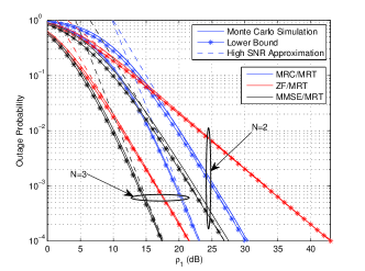
(a) Outage probability

(b) Ergodic capacity

Figure 2: Impact of $N$ on the system performance.

Fig. 2 illustrates the impact of antenna number $N$ on the outage probability and ergodic capacity. It can be readily observed from Fig. 2(a) that for all the three considered schemes, the proposed lower bounds in (27), (39) and (48) are sufficiently tight across the entire SNR range of interest, especially when $N$ is large, and become almost exact in the high SNR region, while the high SNR approximations in (5), (41) and (50) work quite well even at moderate SNR values (i.e., ${\rho_{1}}=20\;\mbox{dB}$). In addition, we see that both the MRC/MRT and MMSE/MRT schemes achieve the full diversity order of $N$, while the ZF/MRT scheme only achieves a diversity order of $N-1$, which is consistent with our analytical results. Moreover, the MMSE/MRT scheme always attains the best outage performance among all three proposed schemes, and the ZF/MRT scheme outperforms the MRC/MRT scheme in the low SNR region, while the opposite holds in the high SNR region.

From Fig. 2(b), we see that, for all three schemes, the proposed ergodic capacity upper bounds in (31), (44) and (53) are sufficiently tight across the entire SNR range of interest. In addition, we observe the intuitive result that increasing $N$ results in an improvement of the ergodic capacity. Moreover, the MMSE/MRT scheme always has the best performance, while the ZF/MRT scheme is slightly inferior, and the performance gap between them disappears as $N$ increases. On the other hand, the MRC/MRT scheme always yields the lowest ergodic capacity, and as $N$ increases, the performance gap becomes more pronounced.

V-B Effect of CCI

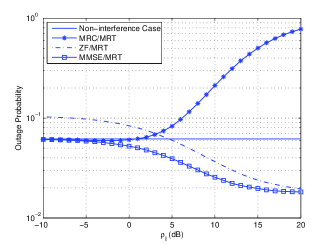
(a) Outage probability

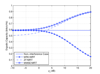
(b) Ergodic capacity

Figure 3: Impact of CCI on the system performance.

Fig. 3 investigates the impact CCI on the system performance. The scenario without CCI is also plotted for comparison. It can be readily observed from Fig. 3(a) that the outage probability of the MRC/MRT scheme decreases slightly for smaller $\rho_{I}$ (i.e., $\rho_{I}<0\mbox{ dB}$), and then increases as the interference becomes stronger. This phenomenon clearly indicates that the CCI can cause either beneficial or harmful effect on the system’s performance. This is because that CCI provides additional energy but at the same time corrupts the desired signal. For the MRC/MRT scheme, when the CCI is too strong, the disadvantage of the CCI becomes the dominant performance limiting factor. However, with sophisticated interference mitigation schemes, e.g., the ZF/MRT and MMSE/MRT schemes, such undesirable effect could be eliminated. As shown in these two schemes, the outage probability decreases monotonically as $\rho_{I}$ increases. Moreover, for the MMSE/MRT scheme, CCI is always desirable, while for the ZF/MRT scheme, whether CCI is beneficial or not depends on its power.

V-C Effect of the Distance

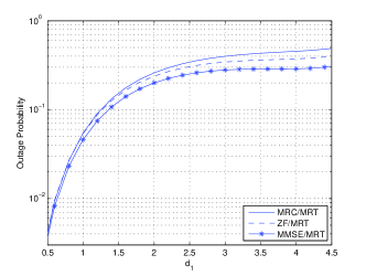
(a) Impact of relay location, $d_{2}=5-d_{1}$, $d_{I}=3$.

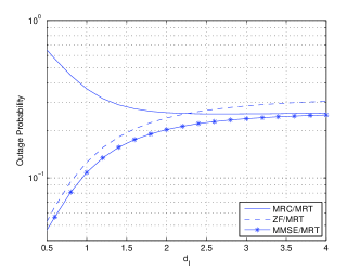
(b) Impact of interferer location, $d_{1}=2$, $d_{2}=3$.

Figure 4: Impact of distance on the system performance.

Fig. 4 shows the effect of the node distances on the system’s outage probability. Unlike the conventional dual-hop system, where it is in general desirable to place the relay in the middle of the source and the destination, Fig. 4(a) indicates that in the energy harvesting scenario, the optimal relay location tends to be close to the source. This observation implies that, the quality of the first hop channel is more important than that of the second hop channel. This is quite intuitive since the quality of the first hop channel not only affects the received signal power at the relay but also determines the available power for the second hop transmission. As shown in Fig. 4(b), as the distance of the CCI increases, the outage performance of ZF/MRT and MMSE/MRT schemes deteriorates. In contrast, the outage performance of the MRC/MRT scheme improves. This is also intuitive, since increasing the distance reduces the received power at the relay, which in turn deteriorates the performance of the ZF/MRT and MMSE/MRT schemes, since strong CCI is desirable for the both the ZF/MRT and MMSE/MRT schemes as illustrated in Fig. 3.

V-D Effect of Power Splitting Ratio $\theta$

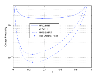
(a) Outage probability

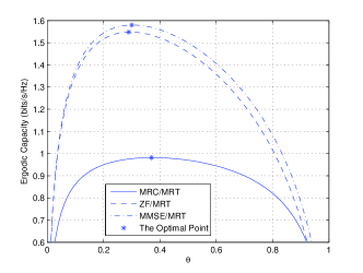
(b) Ergodic capacity

Figure 5: The optimal power splitting ratio $\theta$.

Fig. 5 investigates the the impact of the power splitting ratio $\theta$ on the outage performance. We observe that there exists a unique $\theta$ which gives the best outage or ergodic capacity performance. For all three schemes, we see a similar trends on the impact of $\theta$, i.e., when $\theta$ increases from zero to the optimal value, the performance improves; when $\theta$ exceeds the optimal values, the performance deteriorates gradually. This phenomenon is rather intuitive, since performance of dual-hop systems is limited by the weakest hop quality. Moreover, we see that the optimal $\theta$ is in general different for different schemes and performance metrics, as shown in Fig. 5(a), the MMSE/MRT scheme requires a smaller $\theta$ compared with the MRC/MRT scheme, and the capacity optimal $\theta$ is larger than the outage optimal $\theta$ for the MMSE/MRT scheme.

V-E Effect of Key System Parameters on the Optimal $\theta$

Fig. 6 examines the effect of various key system parameters such as $\eta$, $N$, $\rho_{1}$ and $\rho_{I}$ on the choice of optimal $\theta$. Specifically, Fig. 6(a) illustrates the effect of $\eta$, and we can see that, the outage optimal $\theta$ is a decreasing function of $\eta$. A large $\eta$ implies higher energy conversion efficiency, which in turn suggests that less portion of the signal is needed for energy harvesting, hence, a smaller $\theta$ is required. A similar trend is observed in Fig. 6(b) on the impact of $N$. As $N$ increases, the additional antennas improve the energy harvesting capability, i.e., more energy could be harvested, which implies that the optimal $\theta$ should decrease. The effect of $\rho_{1}$ is shown in Fig. 6(c), it is interesting to see that, for the MRC/MRT and MMSE/MRT schemes, the optimal $\theta$ is an increasing function of $\rho_{1}$, while for the ZF/MRT scheme, the optimal $\theta$ increases first along $\rho_{1}$ and decreases when $\rho_{1}$ exceeds certain value. Finally, Fig. 6(d) investigates the effect of $\rho_{I}$. For all three schemes, the optimal $\theta$ is a decreasing function of $\rho_{I}$. This is intuitive since the CCI serves as the energy source, when the CCI power increases, a smaller $\theta$ is sufficient to fulfill the energy requirement at the relay. Similar trends could be observed for the capacity optimal $\theta$, which are not presented here due to space limitation.

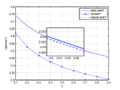
(a) $N=2$, $\rho_{1}=10\;{\mbox{dB}}$, $\rho_{I}=0\;{\mbox{dB}}$

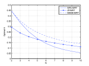
(b) $\eta=0.8$, $\rho_{1}=10\;{\mbox{dB}}$, $\rho_{I}=0\;{\mbox{dB}}$

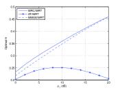
(c) $N=2$, $\eta=0.8$, $\rho_{I}=5\;{\mbox{dB}}$

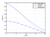
(d) $N=2$, $\eta=0.8$, $\rho_{1}=15\;{\mbox{dB}}$

Figure 6: The impact of (a) $\eta$, (b) $N$, (c) $\rho_{1}$, (d) $\rho_{I}$ on the outage optimal $\theta$.

VI Conclusion

In this paper, we studied the performance of a dual-hop AF energy harvesting system with multiple antennas and CCI. Analytical expressions for the outage probability, ergodic capacity, as well as the diversity order were presented, which provide efficient means for the evaluation of the system’s performance. In addition, the optimal power splitting ratio minimizing the outage probability was analytically characterized while the capacity optimal power splitting ratio was studied numerically. Moreover, the impact of various key system parameters, such as $\eta$, $N$, $\rho_{1}$ and $\rho_{I}$ on the optimal $\theta$ were examined, which provided useful design insights on the choice of a proper power splitting ratio under different system configurations.

Our results demonstrate that both the MRC/MRT and MMSE/MRT schemes achieve a full diversity of $N$ while the ZF/MRT scheme only attains a diversity order of $N-1$. We showed that the CCI could be potentially exploited to significantly improve the system’s performance. With the MMSE/MRT scheme, the CCI is always a desirable factor, and the stronger the CCI, the better the performance. Nevertheless, this is not the case for the MRC/MRT and ZF/MRT schemes, where the CCI could be detrimental. For instance, strong interference degrades the system performance of the MRC/MRT scheme, whereas the performance worsens in the presence of weak interference with the ZF/MRC scheme.

Appendix A Proof of Corollary 1

We first notice that the end-to-end SNR of the system can be tightly upper bounded by

$$\gamma<\frac{\frac{\eta\theta\left({1-\theta}\right)\rho_{1}^{2}}{d_{1}^{2\tau}d_{2}^{\tau}}\left\|{{{\bf{h}}_{2}}}\right\|_{F}^{2}\left\|{{{\bf{h}}_{1}}}\right\|_{F}^{4}}{\frac{\eta\theta{\rho_{1}}}{d_{1}^{\tau}d_{2}^{\tau}}\left\|{{{\bf{h}}_{2}}}\right\|_{F}^{2}\left\|{{{\bf{h}}_{1}}}\right\|_{F}^{2}+\frac{\left({1-\theta}\right){\rho_{1}}}{d_{1}^{\tau}}\left\|{{{\bf{h}}_{1}}}\right\|_{F}^{2}}.$$ (57)

Hence, we get the following the outage probability lower bound:

$$P_{{\sf{out}}}^{{\sf{low}}} ={\rm{Prob}}\left({\left\|{{{\bf{h}}_{2}}}\right\|_{F}^{2}\left({c\left\|{{{\bf{h}}_{1}}}\right\|_{F}^{4}-d\left\|{{{\bf{h}}_{1}}}\right\|_{F}^{2}}\right)<a\left\|{{{\bf{h}}_{1}}}\right\|_{F}^{2}}\right),$$ (58)

which can be computed as

$$P_{{\sf{out}}}^{{\sf{low}}}=\int_{0}^{d/c}{{f_{\left\|{{{\bf{h}}_{1}}}\right\|_{F}^{2}}}\left(x\right)dx}+\\ \int_{d/c}^{\infty}{{f_{\left\|{{{\bf{h}}_{1}}}\right\|_{F}^{2}}}\left(x\right){F_{\left\|{{{\bf{h}}_{2}}}\right\|_{F}^{2}}}\left({\frac{a}{{cx-d}}}\right)dx}.$$ (59)

Noticing that $\left\|{{{\bf{h}}_{1}}}\right\|_{F}^{2}$ and $\left\|{{{\bf{h}}_{2}}}\right\|_{F}^{2}$ are i.i.d. gamma random variables, we have

$$P_{{\sf{out}}}^{{\sf{low}}}=1-\int_{d/c}^{\infty}{\frac{{\Gamma\left({N,\frac{a}{{cx-d}}}\right)}}{{\Gamma\left(N\right)}}\frac{{{x^{N-1}}}}{{\Gamma\left(N\right)}}{e^{-x}}dx}.$$ (60)

Then, making a change of variable $cx-d=t$, (60) can be alternatively written as

$$P_{{\sf{out}}}^{{\sf{low}}}=1-{\left({\frac{1}{c}}\right)^{N}}{e^{-d/c}}\int_{0}^{\infty}{\frac{{\Gamma\left({N,a/t}\right)}}{{\Gamma\left(N\right)}}{{\left({t+d}\right)}^{N-1}}{e^{-t/c}}dt}.$$ (61)

Invoking the series expansion of incomplete gamma function [24, Eq. (8.352.4)] and applying the binomial expansion ${\left({t+d}\right)^{N-1}}=\sum\limits_{j=0}^{N-1}{{{N-1}\choose j}{t^{j}}{d^{N-j-1}}}$, (61) can be further expressed as

$$P_{{\sf{out}}}^{{\sf{low}}}=1-{\left({\frac{1}{c}}\right)^{N}}{e^{-d/c}}\sum\limits_{i=0}^{N-1}{\frac{{{a^{i}}}}{{i!}}}\sum\limits_{j=0}^{N-1}{{{N-1}\choose j}}{d^{N-j-1}}\\ \times\int_{0}^{\infty}{{t^{j-i}}{e^{-\left({\frac{a}{t}+\frac{t}{c}}\right)}}dt}.$$ (62)

To this end, with the help of [24, Eq. (8.432.7)], the desired result can be obtained.

Appendix B Proof of Theorem 2

Starting from (III), we observe that, as ${\rho_{1}}\to\infty$, the end-to-end SNR can be tightly bounded by

$$\gamma<\gamma^{\sf up}=\min\left({\frac{\left({1-\theta}\right){\rho_{1}}}{d_{1}^{\tau}}\left\|{{{\bf{h}}_{1}}}\right\|_{F}^{2}\;,\;\frac{\eta\theta{\rho_{1}}}{d_{1}^{\tau}d_{2}^{\tau}}\left\|{{{\bf{h}}_{2}}}\right\|_{F}^{2}\left\|{{{\bf{h}}_{1}}}\right\|_{F}^{2}}\right).$$ (63)

We now study the c.d.f. of $\gamma^{\sf up}$. Noticing that $\gamma^{\sf up}=\frac{\rho_{1}}{d_{1}^{\tau}}\left\|{{{\bf{h}}_{1}}}\right\|_{F}^{2}{Y}$, where $Y=\min\left({\left({1-\theta}\right)\;,\;\frac{\eta\theta}{d_{2}^{\tau}}\left\|{{{\bf{h}}_{2}}}\right\|_{F}^{2}}\right)$, we first look at the c.d.f. of $Y$, which can be expressed as

$${F_{Y}}\left(y\right)=\underbrace{{\rm{Prob}}\left({\left\|{{{\bf{h}}_{2}}}\right\|_{F}^{2}<\frac{yd_{2}^{\tau}}{{\eta\theta}}\;,\;\left\|{{{\bf{h}}_{2}}}\right\|_{F}^{2}<\frac{(1-\theta)d_{2}^{\tau}}{{\eta\theta}}}\right)}_{{{\rm{P}}_{1}}}+\\ \underbrace{{\rm{Prob}}\left({1-\theta<y\;,\;\left\|{{{\bf{h}}_{2}}}\right\|_{F}^{2}>\frac{(1-\theta)d_{2}^{\tau}}{{\eta\theta}}}\right)}_{{{\rm{P}}_{2}}},$$ (64)

with

$${{\rm{P}}_{1}}=\left\{{\begin{array}[]{*{20}{c}}{{\rm{Prob}}\left({\left\|{{{\bf{h}}_{2}}}\right\|_{F}^{2}<\frac{{(1-\theta)d_{2}^{\tau}}}{{\eta\theta}}}\right)\;,\;y>1-\theta}\\ {{\rm{Prob}}\left({\left\|{{{\bf{h}}_{2}}}\right\|_{F}^{2}<\frac{yd_{2}^{\tau}}{{\eta\theta}}}\right)\;,\;\;\;\;y<1-\theta}\end{array}}\right.,$$ (67)

$$\mbox{\quad}{{\rm{P}}_{2}}=\left\{{\begin{array}[]{*{20}{c}}{{\rm{Prob}}\left({\left\|{{{\bf{h}}_{2}}}\right\|_{F}^{2}>\frac{(1-\theta)d_{2}^{\tau}}{{\eta\theta}}}\right)\;,\;\;y>1-\theta}\\ {0\;,\;\;\;\;\;\;\;\;\;\;\;\;\;\;\;\;\;\;\;\;\;\;\;\;\;\;\;\;\;\;\;\;\;y<1-\theta}\end{array}}\right..$$ (70)

Therefore, the c.d.f. of $Y$ can be finally expressed as

$${F_{Y}}\left(y\right) =\left\{{\begin{array}[]{*{20}{c}}{1\;,\;\;\;\;\;\;\;\;\;\;\;\;\;\;\;\;\;\;\;\;\;\;\;\;y>1-\theta}\\ {{\rm{Prob}}\left({\left\|{{{\bf{h}}_{2}}}\right\|_{F}^{2}<\frac{yd_{2}^{\tau}}{{\eta\theta}}}\right)\;,\;y<1-\theta}\end{array}}\right.$$ (73)

$$=\;\left\{{\begin{array}[]{*{20}{c}}{1\;,\;\;\;\;\;\;\;\;\;\;\;\;\;\;\;\;\;\;\;\;y>1-\theta}\\ {1-\frac{{\Gamma\left({N,{yd_{2}^{\tau}\mathord{\left/{\vphantom{y{\eta\theta}}}\right.\kern-1.2pt}{\eta\theta}}}\right)}}{{\Gamma\left(N\right)}}\;,\;y<1-\theta}\end{array}}\right.$$ (76)

Having obtained the c.d.f. of $Y$, we are ready to compute the c.d.f. of $\gamma^{\sf up}$ as follows:

$${F_{\gamma^{\sf up}}}\left(z\right)=\int_{0}^{\infty}{{F_{Y}}\left({\frac{zd_{1}^{\tau}}{{{\rho_{1}}x}}}\right){f_{\left\|{{{\bf{h}}_{1}}}\right\|_{F}^{2}}}\left(x\right)dx},$$ (77)

which can be expressed as

$${F_{\gamma^{\sf up}}}\left(z\right) =1-\int_{\frac{zd_{1}^{\tau}}{{\left({1-\theta}\right){\rho_{1}}}}}^{\infty}{\frac{{\Gamma\left({N,\frac{zd_{1}^{\tau}d_{2}^{\tau}}{{\eta\theta{\rho_{1}}x}}}\right)}}{{\Gamma\left(N\right)}}\frac{{{x^{N-1}}{e^{-x}}}}{{\Gamma\left(N\right)}}dx}.$$ (78)

Now, applying the asymptotic expansion of incomplete gamma function [24, Eq. (8.354.2)] to (78) yields

$${F_{\gamma^{\sf up}}}\left(z\right)\approx 1-\int_{\frac{zd_{1}^{\tau}}{{\left({1-\theta}\right){\rho_{1}}}}}^{\infty}{\left({1-\frac{1}{{N!}}{{\left({\frac{zd_{1}^{\tau}d_{2}^{\tau}}{{\eta\theta{\rho_{1}}x}}}\right)}^{N}}}\right)\frac{{{x^{N-1}}{e^{-x}}}}{{\Gamma\left(N\right)}}dx}.$$ (79)

Please note, due to the omission of the higher order items of the asymptotic expansion of incomplete gamma function, the expression given in (79) is no longer a bound, but a very tight asymptotic approximation, and matches well with the exact value in the high SNR region, i.e., $P_{\sf out}^{\infty}\mathop{\to}\limits_{{\rho_{1}}\to\infty}{\rm{Prob}}\left({\gamma<\gamma_{\sf th}}\right)$.

To this end, with the help of [24, Eq. (8.350.2)] and [24, Eq. (8.211.1)], we obtain the following closed-form expression for $P_{\sf out}^{\infty}$

$$P_{\sf out}^{\infty}=1-\frac{{\Gamma\left({N,\frac{\gamma_{\sf th}d_{1}^{\tau}}{{\left({1-\theta}\right){\rho_{1}}}}}\right)}}{{\Gamma\left(N\right)}}-\frac{{{\rm{Ei}}\left({-\frac{\gamma_{\sf th}d_{1}^{\tau}}{{\left({1-\theta}\right){\rho_{1}}}}}\right)}}{{N!\left({N-1}\right)!}}{\left({\frac{\gamma_{\sf th}d_{1}^{\tau}d_{2}^{\tau}}{{\eta\theta{\rho_{1}}}}}\right)^{N}}.$$ (80)

Finally, applying [24, Eq. (8.214.1)] and [24, Eq. (8.354.2)] yields the desired result.

Appendix C Proof of Theorem 3

The ergodic capacity can be upper bounded by

$${C_{\sf up}}={C_{{\gamma_{1}}}}+{C_{{\gamma_{2}}}}-\frac{1}{2}{\log_{2}}\left({1+{e^{{\mathop{\rm E}\nolimits}\left({\ln{\gamma_{1}}}\right)}}+{e^{{\mathop{\rm E}\nolimits}\left({\ln{\gamma_{2}}}\right)}}}\right).$$ (81)

Note that ${C_{{\gamma_{1}}}}$ is the ergodic capacity of the SIMO Rayleigh channel, which has been given in [37] as

$${C_{{\gamma_{1}}}}=\frac{1}{{2\ln 2}}\sum\limits_{k=0}^{N-1}{{{\left({\frac{d_{1}^{\tau}}{{\left({1-\theta}\right){\rho_{1}}}}}\right)}^{k}}{e^{\frac{d_{1}^{\tau}}{{\left({1-\theta}\right){\rho_{1}}}}}}\Gamma\left({-k,\frac{d_{1}^{\tau}}{{\left({1-\theta}\right){\rho_{1}}}}}\right)},$$ (82)

and ${C_{{\gamma_{2}}}}$ is the ergodic capacity of the SIMO keyhole channel, which has been given in [38] as

$${C_{{\gamma_{2}}}}=\frac{1}{{2\ln 2}}\frac{1}{{\Gamma\left({{N}}\right)}}\sum\limits_{m=0}^{N-1}{\frac{{\left({\frac{d_{1}^{\tau}d_{2}^{\tau}}{{\eta\theta{\rho_{1}}}}}\right)}^{m}}{{m!}}G_{1,3}^{3,1}\left(\frac{d_{1}^{\tau}d_{2}^{\tau}}{{\eta\theta{\rho_{1}}}}\middle|^{-m}_{-m,N-m,0}\right)}.$$ (83)

Next, we observe that ${\mathop{\rm E}\nolimits}\left({\ln{\gamma_{1}}}\right)=\ln\left({\frac{\left({1-\theta}\right){\rho_{1}}}{d_{1}^{\tau}}}\right)+{\mathop{\rm E}\nolimits}\left({\ln\left\|{{{\bf{h}}_{1}}}\right\|_{F}^{2}}\right)$ and ${\mathop{\rm E}\nolimits}\left({\ln{\gamma_{2}}}\right)=\ln\left({\frac{\eta\theta{\rho_{1}}}{d_{1}^{\tau}d_{2}^{\tau}}}\right)+{\mathop{\rm E}\nolimits}\left({\ln\left\|{{{\bf{h}}_{1}}}\right\|_{F}^{2}}\right)+{\mathop{\rm E}\nolimits}\left({\ln\left\|{{{\bf{h}}_{2}}}\right\|_{F}^{2}}\right)$. It is easy to show that

$${\mathop{\rm E}\nolimits}\left({\ln\left\|{{{\bf{h}}_{1}}}\right\|_{F}^{2}}\right)={\mathop{\rm E}\nolimits}\left({\ln\left\|{{{\bf{h}}_{2}}}\right\|_{F}^{2}}\right)=\psi\left(N\right).$$ (84)

To this end, pulling everything together yeilds the desired result.

Appendix D Proof of Theorem 4

From (26), the outage lower bound can be evaluated as

$$P_{I\sf out}^{\sf LMRC} ={\rm{Prob}}\left({{\gamma_{I1}^{\sf MRC}}<{\gamma_{{\sf{th}}}}}\right)+{\rm{Prob}}\left({{\gamma_{I2}^{\sf MRC}}<{\gamma_{{\sf{th}}}}}\right)$$

$$-{\rm{Prob}}\left({{\gamma_{I1}^{\sf MRC}}<{\gamma_{{\sf{th}}}}\;\text{and}\;{\gamma_{I2}^{\sf MRC}}<{\gamma_{{\sf{th}}}}}\right)$$

$$\approx{\rm{Prob}}\left({{\gamma_{I1}^{\sf MRC}}<{\gamma_{{\sf{th}}}}}\right)+{\rm{Prob}}\left({{\gamma_{I2}^{\sf MRC}}<{\gamma_{{\sf{th}}}}}\right)$$

$$-{\rm{Prob}}\left({{\gamma_{I1}^{\sf MRC}}<{\gamma_{{\sf{th}}}}}\right){\rm{Prob}}\left({{\gamma_{I2}^{\sf MRC}}<{\gamma_{{\sf{th}}}}}\right).$$ (85)

In general, $\gamma_{I1}^{\sf MRC}$ and $\gamma_{I2}^{\sf MRC}$ are not independent. However, through Monte Carlo simulations, we observe that as long as $\rho_{I}$ is close to $\rho_{1}$, the term ${\rm{Prob}}\left({{\gamma_{I1}^{\sf MRC}}<{\gamma_{{\sf{th}}}}\;\text{and}\;{\gamma_{I2}^{\sf MRC}}<{\gamma_{{\sf{th}}}}}\right)$ can be safely approximated by ${\rm{Prob}}\left({{\gamma_{I1}^{\sf MRC}}<{\gamma_{{\sf{th}}}}}\right){\rm{Prob}}\left({{\gamma_{I2}^{\sf MRC}}<{\gamma_{{\sf{th}}}}}\right)$ in the whole SNR region as shown in Fig 7(a). As a matter of fact, the same approximation has been adopted in [39]. Therefore, the remaining task is to compute ${\rm{Prob}}\left({{\gamma_{I1}^{\sf MRC}}<{\gamma_{{\sf{th}}}}}\right)$ and ${\rm{Prob}}\left({{\gamma_{I2}^{\sf MRC}}<{\gamma_{{\sf{th}}}}}\right)$.

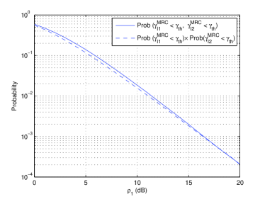
(a) Probability versus $\rho_{1}$ in dB.

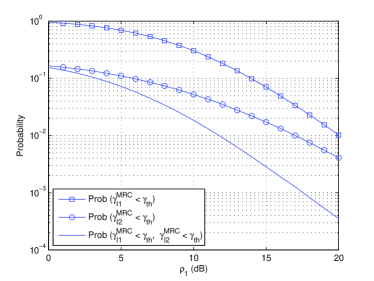
(b) Probability versus $\rho_{1}$ in dB.

Figure 7: Justification of the approximations employed in the proof of Theorem 4 and 5.

The c.d.f. of ${\gamma_{I1}^{\sf MRC}}$ can be expressed as

$$F_{\gamma_{I1}^{\sf MRC}}\left({\gamma_{\sf th}}\right)={\rm{Prob}}\left({\left\|{{{\bf{h}}_{1}}}\right\|_{F}^{2}<\frac{\left({U+1}\right)d_{1}^{\tau}{\gamma_{{\sf{th}}}}}{{\left({1-\theta}\right){\rho_{1}}}}}\right),$$ (86)

where $U=\frac{\left({1-\theta}\right){\rho_{I}}}{d_{I}^{\tau}}\frac{{{{\left|{{\bf{h}}_{1}^{\dagger}{{\bf{h}}_{I}}}\right|}^{2}}}}{{\left\|{{{\bf{h}}_{1}}}\right\|_{F}^{2}}}$, which is an exponential random variables with parameter $\frac{\left({1-\theta}\right){\rho_{I}}}{d_{I}^{\tau}}$ [34]. Hence, we have

$$F_{\gamma_{I1}^{\sf MRC}}\left({\gamma_{\sf th}}\right)=1-\frac{{{d_{I}^{\tau}e^{-\frac{{{d_{1}^{\tau}\gamma_{{\sf{th}}}}}}{{\left({1-\theta}\right){\rho_{1}}}}}}}}{{\left({1-\theta}\right){\rho_{I}}}}{\sum\limits_{m=0}^{N-1}{\frac{1}{{m!}}\left({\frac{d_{1}^{\tau}\gamma_{{\sf{th}}}}{{\left({1-\theta}\right){\rho_{1}}}}}\right)}^{m}}\\ \times\int_{0}^{\infty}{{{\left({x+1}\right)}^{m}}{e^{-\left({\frac{d_{1}^{\tau}\gamma_{{\sf{th}}}}{{\left({1-\theta}\right){\rho_{1}}}}+\frac{d_{I}^{\tau}}{{\left({1-\theta}\right){\rho_{I}}}}}\right)x}}dx}.$$ (87)

Then, applying the binomial expansion and invoking [24, Eq. (8.312.2)], we arrive at

$$F_{\gamma_{I1}^{\sf MRC}}\left({\gamma_{\sf th}}\right)=1-\frac{{{d_{I}^{\tau}e^{-\frac{{{d_{1}^{\tau}\gamma_{{\sf{th}}}}}}{{\left({1-\theta}\right){\rho_{1}}}}}}}}{{\left({1-\theta}\right){\rho_{I}}}}{\sum\limits_{m=0}^{N-1}{\left({\frac{{{d_{1}^{\tau}\gamma_{{\sf{th}}}}}}{{\left({1-\theta}\right){\rho_{1}}}}}\right)}^{m}}\\ \times\sum\limits_{n=0}^{m}{\frac{1}{{(m-n)!}}{{\left({\frac{{\left({1-\theta}\right){\rho_{1}}{\rho_{I}}}}{{{d_{I}^{\tau}\rho_{1}}+{d_{1}^{\tau}\rho_{I}}{\gamma_{{\sf{th}}}}}}}\right)}^{n+1}}}.$$ (88)

Similarly, the c.d.f. of ${\gamma_{I2}^{\sf MRC}}$ can be expressed as

$$F_{\gamma_{I2}^{\sf MRC}}\left({\gamma_{\sf th}}\right) ={\rm{Prob}}\left({{\gamma_{I2}^{\sf MRC}}<{\gamma_{{\sf{th}}}}}\right)={\rm{Prob}}\left({\left\|{{{\bf{h}}_{2}}}\right\|_{F}^{2}<\frac{{{d_{2}^{\tau}\gamma_{{\sf{th}}}}}}{{\eta\theta Z}}}\right)$$

$$=\int_{0}^{\infty}{{F_{\left\|{{{\bf{h}}_{2}}}\right\|_{F}^{2}}}\left({\frac{{{d_{2}^{\tau}\gamma_{{\sf{th}}}}}}{{\eta\theta x}}}\right){f_{Z}}\left(x\right)dx},$$ (89)

where $Z=\frac{\rho_{1}}{d_{1}^{\tau}}\left\|{{{\bf{h}}_{1}}}\right\|_{F}^{2}+\frac{\rho_{I}}{d_{I}^{\tau}}\left\|{{{\bf{h}}_{I}}}\right\|_{F}^{2}$, which is a sum of two independent gamma random variables. According to [35], if ${\rho_{1}}\neq{\rho_{I}}$ the probability density function (p.d.f.) of $Z$ can be given by

$${f_{Z}}(x)=\frac{d_{1}^{N\tau}d_{I}^{N\tau}}{{\rho_{1}^{N}\rho_{I}^{N}}}\sum\limits_{s=1}^{N}{\frac{{\prod\nolimits_{j=1}^{s-1}{\left({1-N-j}\right)}}}{{\left({N-s}\right)!\left({s-1}\right)!}}}\times\\ {{\left({\frac{d_{I}^{\tau}}{{{\rho_{I}}}}-\frac{d_{1}^{\tau}}{{{\rho_{1}}}}}\right)}^{1-N-s}}{x^{N-s}}{e^{-\frac{d_{1}^{\tau}x}{{{\rho_{1}}}}}}+\frac{d_{1}^{N\tau}d_{I}^{N\tau}}{{\rho_{1}^{N}\rho_{I}^{N}}}\times\\ \sum\limits_{s=1}^{N}{\frac{{\prod\nolimits_{j=1}^{s-1}{\left({1-N-j}\right)}}}{{\left({N-s}\right)!\left({s-1}\right)!}}{{\left({\frac{d_{1}^{\tau}}{{{\rho_{1}}}}-\frac{d_{I}^{\tau}}{{{\rho_{I}}}}}\right)}^{1-N-s}}{x^{N-s}}{e^{-\frac{d_{I}^{\tau}x}{{{\rho_{I}}}}}}}.$$ (90)

After some algebraic manipulations and with the help of [24, Eq. ( 8.432.7)], (D) can be computed as (91) shown on the top of the next page.

$$F_{\gamma_{I2}^{\sf MRC}}\left({\gamma_{\sf th}}\right)=1-\frac{2d_{1}^{N\tau}d_{I}^{N\tau}}{{\rho_{1}^{N}\rho_{I}^{N}}}\sum\limits_{s=1}^{N}{\frac{{\prod\nolimits_{j=1}^{s-1}{\left({1-N-j}\right)}}}{{\left({N-s}\right)!\left({s-1}\right)!}}{{\left({\frac{d_{I}^{\tau}}{{{\rho_{I}}}}-\frac{d_{1}^{\tau}}{{{\rho_{1}}}}}\right)}^{1-N-s}}}\sum\limits_{m=0}^{N-1}\frac{1}{{m!}}{{\left({\frac{{{d_{2}^{\tau}\gamma_{\sf th}}}}{{\eta\theta}}}\right)}^{N+1-s}}\times\\ {{\left({\frac{{{d_{1}^{\tau}d_{2}^{\tau}\gamma_{\sf th}}}}{{\eta\theta{\rho_{1}}}}}\right)}^{\frac{{m+s-N-1}}{2}}}{K_{m+s-N-1}}\left({2\sqrt{\frac{{{d_{1}^{\tau}d_{2}^{\tau}\gamma_{\sf th}}}}{{\eta\theta{\rho_{1}}}}}}\right)+\frac{2d_{1}^{N\tau}d_{I}^{N\tau}}{{\rho_{1}^{N}\rho_{I}^{N}}}\sum\limits_{s=1}^{N}{\frac{{\prod\nolimits_{j=1}^{s-1}{\left({1-N-j}\right)}}}{{\left({N-s}\right)!\left({s-1}\right)!}}}\times\\ {{\left({\frac{d_{1}^{\tau}}{{{\rho_{1}}}}-\frac{d_{I}^{\tau}}{{{\rho_{I}}}}}\right)}^{1-N-s}}\sum\limits_{m=0}^{N-1}{\frac{1}{{m!}}{{\left({\frac{{d_{2}^{\tau}\gamma_{\sf th}}}{{\eta\theta}}}\right)}^{N+1-s}}{{\left({\frac{{{d_{2}^{\tau}d_{I}^{\tau}\gamma_{\sf th}}}}{{\eta\theta{\rho_{I}}}}}\right)}^{\frac{{m+s-N-1}}{2}}}{K_{m+s-N-1}}\left({2\sqrt{\frac{{{d_{2}^{\tau}d_{I}^{\tau}\gamma_{\sf th}}}}{{\eta\theta{\rho_{I}}}}}}\right)}.$$ (91)

 

To this end, substituting (88) and (91) into (D) yields the desired result.

Appendix E Proof of Theorem 5

When ${\rho_{1}}\to\infty$ the outage probability of the system can be approximated as

$${P_{I\sf out}^{\sf MRC}}\approx{\rm{Prob}}\left({{\gamma_{I1}^{\sf MRC}}<{\gamma_{{\sf{th}}}}}\right)+{\rm{Prob}}\left({{\gamma_{I2}^{\sf MRC}}<{\gamma_{{\sf{th}}}}}\right).$$ (92)

This approximation comes from the fact that, as $\rho_{1}$ increases, ${\rm{Prob}}\left({{\gamma_{I1}^{\sf MRC}}<{\gamma_{{\sf{th}}}}\;\text{and}\;{\gamma_{I2}^{\sf MRC}}<{\gamma_{{\sf{th}}}}}\right)$ is negligible compared with ${\rm{Prob}}\left({{\gamma_{I1}^{\sf MRC}}<{\gamma_{{\sf{th}}}}}\right)$ or ${\rm{Prob}}\left({{\gamma_{I2}^{\sf MRC}}<{\gamma_{{\sf{th}}}}}\right)$ (it can be justified through Fig 7(b)).

Therefore, the high SNR approximation for the outage probability can be given by

$$P_{I\sf out}^{\sf MRC}\approx F_{\gamma_{I1}^{\sf MRC}}^{\infty}\left({\gamma_{\sf th}}\right)+F_{\gamma_{I2}^{\sf MRC}}^{\infty}\left({\gamma_{\sf th}}\right),$$ (93)

where $F_{\gamma_{I1}^{\sf MRC}}^{\infty}$ and $F_{\gamma_{I2}^{\sf MRC}}^{\infty}$ denote the high SNR approximation of ${\rm{Prob}}\left({{\gamma_{I1}^{\sf MRC}}<{\gamma_{{\sf{th}}}}}\right)$ and ${\rm{Prob}}\left({{\gamma_{I2}^{\sf MRC}}<{\gamma_{{\sf{th}}}}}\right)$, respectively.

We start with the characterization of $F_{\gamma_{I1}^{\sf MRC}}^{\infty}$. Starting from (86), and with the help of the asymptotic expansion of incomplete gamma function, we have

$$F_{\gamma^{\sf MRC}_{I1}}^{\infty}\left({\gamma_{\sf th}}\right)={\left({\frac{{{d_{1}^{\tau}\gamma_{{\sf{th}}}}}}{{\left({1-\theta}\right){\rho_{1}}}}}\right)^{N}}\sum\limits_{n=0}^{N}{\frac{{{{\left({\left({1-\theta}\right){\rho_{I}}}\right)}^{n}}}}{{d_{I}^{n\tau}\left({N-n}\right)!}}}.$$ (94)

Now, we turn our attention to $F_{\gamma_{I2}^{\sf MRC}}^{\infty}\left({\gamma_{\sf th}}\right)$. According to (D) and utilizing the the asymptotic expansion of incomplete gamma function, conditioned on $y_{1}=\frac{\rho_{1}}{d_{1}^{\tau}}\left\|{{{\bf{h}}_{1}}}\right\|_{F}^{2}$ and $y_{I}=\frac{\rho_{I}}{d_{I}^{\tau}}\left\|{{{\bf{h}}_{I}}}\right\|_{F}^{2}$, $F_{\gamma_{I2}^{\sf MRC}}^{\infty}\left({\gamma_{\sf th}}\right)$ can be expressed as

$$F_{\gamma_{I2}^{\sf MRC}}^{\infty}\left({\gamma_{\sf th}}\right)=\frac{1}{{\Gamma\left({N+1}\right)}}{\left({\frac{{{d_{2}^{\tau}\gamma_{{\sf{th}}}}}}{{\eta\theta\left({{y_{1}}+{y_{I}}}\right)}}}\right)^{N}}.$$ (95)

Averaging over ${y_{I}}$, we have

$$F_{\gamma_{I2}^{\sf MRC}}^{\infty}\left({\gamma_{\sf th}}\right)=\frac{1}{{\Gamma\left({N+1}\right)\Gamma\left(N\right)}}{\left({\frac{{{d_{I}^{\tau}d_{2}^{\tau}\gamma_{{\sf{th}}}}}}{{\eta\theta{\rho_{I}}}}}\right)^{N}}\times\\ \int_{0}^{\infty}{{{\left({\frac{1}{{{y_{1}}+x}}}\right)}^{N}}{x^{N-1}}{e^{-\frac{xd_{I}^{\tau}}{{{\rho_{I}}}}}}dx}.$$ (96)

Make a change of variable ${y_{1}}+x=t$, and apply the binomial expansion, (96) can be rewritten by

$$F_{\gamma_{I2}^{\sf MRC}}^{\infty}\left({\gamma_{\sf th}}\right)=\frac{{{e^{\frac{{{d_{I}^{\tau}y_{1}}}}{{{\rho_{I}}}}}{\left({\frac{{{d_{2}^{\tau}\gamma_{{\sf{th}}}}}}{{\eta\theta}}}\right)^{N}}}}}{{\Gamma\left({N+1}\right)\Gamma\left(N\right)}}\sum\limits_{i=0}^{N-1}{{N-1\choose i}}{{\left({-{y_{1}}}\right)}^{N-i-1}}\\ \times\left({\frac{\rho_{I}}{d_{I}^{\tau}}}\right)^{i-2N+1}\Gamma\left({i-N+1,\frac{{{d_{I}^{\tau}y_{1}}}}{{{\rho_{I}}}}}\right).$$ (97)

Further averaging over ${y_{1}}$, we have

$$F_{\gamma_{I2}^{\sf MRC}}^{\infty}\left({\gamma_{\sf th}}\right)=\frac{1}{{\Gamma\left({N+1}\right)\Gamma{{\left(N\right)}^{2}}}}{\left({\frac{{{d_{1}^{\tau}d_{2}^{\tau}\gamma_{{\sf{th}}}}}}{{\eta\theta{\rho_{1}}}}}\right)^{N}}\times\\ \sum\limits_{i=0}^{N-1}{{N-1\choose i}{{\left({-1}\right)}^{N-i-1}}\left({\frac{\rho_{I}}{d_{I}^{\tau}}}\right)^{i-2N+1}}\times\\ \underbrace{\int_{0}^{\infty}{{e^{-\left({\frac{d_{1}^{\tau}}{{{\rho_{1}}}}-\frac{d_{I}^{\tau}}{{{\rho_{I}}}}}\right)x}}{x^{2N-i-2}}\Gamma\left({i-N+1,\frac{xd_{I}^{\tau}}{{{\rho_{I}}}}}\right)dx}}_{{\cal I}_{1}}.$$ (98)

With the help of [24, Eq. (6.455.1)], the integral ${{\cal I}_{1}}$ can be solved as

$${{\cal I}_{1}}=\frac{{\left({\frac{\rho_{I}}{d_{I}^{\tau}}}\right)^{N-i-1}\left({\frac{\rho_{1}}{d_{1}^{\tau}}}\right)^{N}\Gamma\left(N\right)}}{{2N-i-1}}\times\\ {}_{2}{F_{1}}\left({1,N;2N-i;1-\frac{{{d_{I}^{\tau}\rho_{1}}}}{{{d_{1}^{\tau}\rho_{I}}}}}\right).$$ (99)

Then, utilizing [24, Eq. (9.131.1)], we can obtain

$$F_{\gamma_{I2}^{\sf MRC}}^{\infty}(\gamma_{\sf th})=\frac{{\left({\frac{{{d_{1}^{\tau}d_{2}^{\tau}\gamma_{{\rm{th}}}}}}{{\eta\theta{\rho_{1}}}}}\right)^{N}}}{{\Gamma(N+1)\Gamma(N)}}\sum\limits_{i=0}^{N-1}{{N-1\choose i}}\times\\ {{\left({-1}\right)}^{N-i-1}}\frac{{{}_{2}{F_{1}}\left({N,2N-i-1;2N-i;1-\frac{{{d_{I}^{\tau}\rho_{I}}}}{{{d_{1}^{\tau}\rho_{1}}}}}\right)}}{{2N-i-1}}.$$ (100)

To this end, substituting (94) and (100) into (93) yields the desired result.

Appendix F Proof of Theorem 6

Similar to the proof of Theorem 3, we note that the ergodic capacity upper bound can be computed as

$${C_{I\sf up}^{\sf MRC}}={C_{{\gamma_{I1}^{\sf MRC}}}}+{C_{{\gamma_{I2}^{\sf MRC}}}}-\\ \frac{1}{2}{\log_{2}}\left({1+{e^{{\mathop{\rm E}\nolimits}\left({\ln{\gamma_{I1}^{\sf MRC}}}\right)}}+{e^{{\mathop{\rm E}\nolimits}\left({\ln{\gamma_{I2}^{\sf MRC}}}\right)}}}\right),$$ (101)

where $C_{\gamma_{Ii}^{\sf MRC}}=\frac{1}{2}{\mathop{\rm E}\nolimits}\left[{{{\log}_{2}}\left({1+{\gamma_{Ii}^{\sf MRC}}}\right)}\right]$, for $k\in\{1,2\}$. Hence, the remaining task is to compute ${C_{{\gamma_{I1}^{\sf MRC}}}}$, ${C_{{\gamma_{I2}^{\sf MRC}}}}$, ${{\mathop{\rm E}\nolimits}\left({\ln{\gamma_{I1}^{\sf MRC}}}\right)}$ and ${{\mathop{\rm E}\nolimits}\left({\ln{\gamma_{I2}^{\sf MRC}}}\right)}$.

F-A Calculation of $C_{\gamma_{I1}^{\sf MRC}}$

Utilizing the same method as in [33] and invoking the c.d.f. of $\gamma_{I1}^{\sf MRC}$ given in (88), $C_{\gamma_{I1}^{\sf MRC}}$ can be computed as

$${C_{{\gamma_{I1}^{\sf MRC}}}}=\frac{1}{{2\ln 2}}\sum\limits_{m=0}^{N-1}{{{\left({\frac{d_{1}^{\tau}}{{\left({1-\theta}\right){\rho_{1}}}}}\right)}^{m}}\sum\limits_{n=0}^{m}{\frac{{{{\left({\left({1-\theta}\right){\rho_{I}}}\right)}^{n}}}}{{d_{I}^{n\tau}\left({m-n}\right)!}}}}\times\\ \underbrace{\int_{0}^{\infty}{\frac{{{e^{-\frac{xd_{1}^{\tau}}{{\left({1-\theta}\right){\rho_{1}}}}}}{x^{m}}}}{{\left({1+x}\right)}}{{\left({1+\frac{{{d_{1}^{\tau}\rho_{I}}}}{{{d_{I}^{\tau}\rho_{1}}}}x}\right)}^{-\left({n+1}\right)}}dx}}_{{\cal{I}}_{2}}.$$ (102)

With the help of the identity ${\left({1+\beta x}\right)^{-\alpha}}=\frac{1}{{\Gamma\left(\alpha\right)}}{\mathop{\rm G}\nolimits}_{1,1}^{1,1}\left({\beta x\left|{}_{0}^{1-\alpha}\right.}\right)$ and the integral formula [36, Eq. (2.6.2)], ${\cal I}_{2}$ can be computed as

$${\cal I}_{2} =\frac{{\left({\left({1-\theta}\right){\rho_{1}}}\right)}^{m+1}}{{d_{1}^{(m+1)\tau}\Gamma\left({n+1}\right)}}{\mathop{\rm G}\nolimits}_{1,[1:1],0,[1:1]}^{1,1,1,1,1}\left({}^{\frac{\left({1-\theta}\right){\rho_{1}}}{d_{1}^{\tau}}}_{\frac{\left({1-\theta}\right){\rho_{I}}}{d_{I}^{\tau}}}\middle|\begin{subarray}{c}{m+1}\\ {0;-n}\\ -\\ {0;0}\end{subarray}\right).$$ (103)

F-B Calculation of $C_{\gamma_{I2}^{\sf MRC}}$

Similarly, with the help of the c.d.f. of $\gamma_{I2}^{\sf MRC}$ given in (91), $C_{\gamma_{I2}^{\sf MRC}}$ can be computed as (104) shown on the top of the next page,

$${C_{{\gamma_{I2}^{\sf MRC}}}}=\frac{d_{1}^{N\tau}d_{I}^{N\tau}}{{\rho_{1}^{N}\rho_{I}^{N}\ln 2}}\sum\limits_{s=1}^{N}{\frac{{\prod\nolimits_{j=1}^{s-1}{\left({1-N-j}\right)}}}{{\left({N-s}\right)!\left({s-1}\right)!}}{{\left({\frac{d_{I}^{\tau}}{{{\rho_{I}}}}-\frac{d_{1}^{\tau}}{{{\rho_{1}}}}}\right)}^{1-N-s}}\sum\limits_{m=0}^{N-1}{\frac{1}{{m!}}{{\left({\frac{d_{2}^{\tau}}{{\eta\theta}}}\right)}^{N+1-s}}{{\cal I}_{3}}}}\\ +\frac{d_{1}^{\tau}d_{I}^{\tau}}{{\rho_{1}^{N}\rho_{I}^{N}\ln 2}}\sum\limits_{s=1}^{N}{\frac{{\prod\nolimits_{j=1}^{s-1}{\left({1-N-j}\right)}}}{{\left({N-s}\right)!\left({s-1}\right)!}}{{\left({\frac{d_{1}^{\tau}}{{{\rho_{1}}}}-\frac{d_{I}^{\tau}}{{{\rho_{I}}}}}\right)}^{1-N-s}}\sum\limits_{m=0}^{N-1}{\frac{1}{{m!}}{{\left({\frac{d_{2}^{\tau}}{{\eta\theta}}}\right)}^{N+1-s}}{{\cal I}_{4}}}},$$ (104)

 

where

$${\cal I}_{3}=\int_{0}^{\infty}{\frac{{{x^{N+1-s}}}}{{1+x}}{{\left({\frac{d_{1}^{\tau}d_{2}^{\tau}x}{{\eta\theta{\rho_{1}}}}}\right)}^{\frac{{m+s-N-1}}{2}}}}\times\\ {K_{m+s-N-1}}\left({2\sqrt{\frac{d_{1}^{\tau}d_{2}^{\tau}x}{{\eta\theta{\rho_{1}}}}}}\right)dx,$$ (105)

and

$${\cal I}_{4}=\int_{0}^{\infty}{\frac{{{x^{N+1-s}}}}{{1+x}}{{\left({\frac{d_{2}^{\tau}d_{I}^{\tau}x}{{\eta\theta{\rho_{I}}}}}\right)}^{\frac{{m+s-N-1}}{2}}}}\times\\ {K_{m+s-N-1}}\left({2\sqrt{\frac{d_{2}^{\tau}d_{I}^{\tau}x}{{\eta\theta{\rho_{I}}}}}}\right)dx.$$ (106)

Then, following the similar lines as in the Appendix C, ${C_{{\gamma_{I2}^{\sf MRC}}}}$ can be expressed in closed-form.

F-C Calculation of ${{\mathop{\rm E}\nolimits}\left({\ln{\gamma_{I1}^{\sf MRC}}}\right)}$

Invoking the c.d.f. of $\gamma_{I1}^{\sf MRC}$, the general moment of $\gamma_{I1}^{\sf MRC}$ can be computed as

$${\rm{E}}\left({(\gamma_{I1}^{\sf MRC})^{k}}\right)=\sum\limits_{m=0}^{N-1}{{{\left({\frac{1}{{\left({1-\theta}\right){\rho_{1}}}}}\right)}^{m}}\sum\limits_{n=0}^{m}{\frac{{{{\left({\left({1-\theta}\right){\rho_{I}}}\right)}^{n}}}}{{\left({m-n}\right)!}}k}}\times\\ \underbrace{\int_{0}^{\infty}{{e^{-\frac{x}{{\left({1-\theta}\right){\rho_{1}}}}}}{x^{m+k-1}}{{\left({1+\frac{{{\rho_{I}}}}{{{\rho_{1}}}}x}\right)}^{-\left({n+1}\right)}}dx}}_{{{\cal I}_{5}}}.$$ (107)

With the help of [24, Eq. (9.211.4)], we obtain

$${\rm{E}}\left({(\gamma_{I1}^{\sf MRC})^{k}}\right)=\sum\limits_{m=0}^{N-1}{{{\left({\frac{d_{1}^{\tau}}{{\left({1-\theta}\right){\rho_{1}}}}}\right)}^{m}}\sum\limits_{n=0}^{m}{\frac{{{{\left({\left({1-\theta}\right){\rho_{I}}}\right)}^{n}}}}{{d_{I}^{n\tau}\left({m-n}\right)!}}}}\times\\ k{\left({\frac{{{d_{I}^{\tau}\rho_{1}}}}{{{d_{1}^{\tau}\rho_{I}}}}}\right)^{m+k}}\Gamma({m+k})\times\\ \Psi\left({m+k,m+k-n;\frac{d_{I}^{\tau}}{{({1-\theta}){\rho_{I}}}}}\right).$$ (108)

The expectation of $\ln{\gamma_{I1}^{\sf MRC}}$ can be derived using ${\mathop{\rm E}\nolimits}\left({\ln x}\right)={\left.{\frac{{d{\mathop{\rm E}\nolimits}\left({{x^{k}}}\right)}}{{dk}}}\right|_{k=0}}$. To proceed, we find it convenient to use (109) (shown on the top of the next page) as an alternative expression of (108)

$${\rm{E}}\left({(\gamma_{I1}^{\sf MRC})^{k}}\right)=\underbrace{{e^{\frac{d_{I}^{\tau}}{{\left({1-\theta}\right){\rho_{I}}}}}}\Gamma\left({k+1}\right){{\left({\frac{{{d_{I}^{\tau}\rho_{1}}}}{{{d_{1}^{\tau}\rho_{I}}}}}\right)}^{k}}\Gamma\left({1-k,\frac{d_{I}^{\tau}}{{\left({1-\theta}\right){\rho_{I}}}}}\right)}_{{s_{1}}\left(k\right)}+\underbrace{\sum\limits_{m=1}^{N-1}{{{\left({\frac{d_{1}^{\tau}}{{\left({1-\theta}\right){\rho_{1}}}}}\right)}^{m}}\sum\limits_{n=0}^{m}{\frac{{{{\left({(1-\theta){\rho_{I}}}\right)}^{n}}}}{{d_{I}^{n\tau}\left({m-n}\right)!}}k{T_{1}}(k)}}}_{{s_{2}}\left(k\right)}.$$ (109)

 

where ${T_{1}}\left(k\right)={\Psi\left({m+k,m+k-n;\frac{d_{I}^{\tau}}{{\left({1-\theta}\right){\rho_{I}}}}}\right){\left({\frac{{{d_{I}^{\tau}\rho_{1}}}}{{{d_{1}^{\tau}\rho_{I}}}}}\right)}^{m+k}}$ $\times\Gamma\left({m+k}\right)$. Now, the expectation of $\ln{\gamma_{I1}^{\sf MRC}}$ can be computed as

$${\mathop{\rm E}\nolimits}\left({\ln{\gamma_{I1}^{\sf MRC}}}\right)={\left.{\frac{{d{s_{1}}\left(k\right)}}{{dk}}}\right|_{k=0}}+{\left.{\frac{{d{s_{2}}\left(k\right)}}{{dk}}}\right|_{k=0}}.$$ (110)

It is easy to show that

$${\left.{\frac{{d{s_{1}}\left(k\right)}}{{dk}}}\right|_{k=0}}=\ln\left({\left({1-\theta}\right){\rho_{1}}}\right)-\ln{d_{1}^{\tau}}+\psi\left(1\right)-\\ {e^{\frac{d_{I}^{\tau}}{{\left({1-\theta}\right){\rho_{I}}}}}}G_{2,3}^{3,0}\left(\frac{d_{I}^{\tau}}{{\left({1-\theta}\right){\rho_{I}}}}\middle|^{1,1}_{0,0,1}\right),$$ (111)

where we have utilized the identity $\Gamma\left({1,\frac{d_{I}^{\tau}}{{\left({1-\theta}\right){\rho_{I}}}}}\right)={e^{-\frac{d_{I}^{\tau}}{{\left({1-\theta}\right){\rho_{I}}}}}}$, and the derivative property $\frac{{d\Gamma\left({a,z}\right)}}{{da}}=\Gamma\left({a,z}\right)\ln z+G_{2,3}^{3,0}\left(z\middle|^{1,1}_{0,0,a}\right)$.

As for ${\left.{\frac{{d{s_{2}}\left(k\right)}}{{dk}}}\right|_{k=0}}$, it is easy to observe that the key task is to compute ${\left.{\frac{{dk{T_{1}}\left(k\right)}}{{dk}}}\right|_{k=0}}$. Hence, we have

$${\left.{\frac{{dk{T_{1}}\left(k\right)}}{{dk}}}\right|_{k=0}}={\left.{{T_{1}}\left(k\right)}\right|_{k=0}}+k{\left.{\frac{{d{T_{1}}\left(k\right)}}{{dk}}}\right|_{k=0}}.$$ (112)

Noticing that when $m\geq 1$, ${\left.{\frac{{d{T_{1}}\left(k\right)}}{{dk}}}\right|_{k=0}}<\infty$ is a constant, we have ${\left.{k\frac{{d{T_{1}}\left(k\right)}}{{dk}}}\right|_{k=0}}=0$, hence ${\left.{\frac{{dk{T_{1}}\left(k\right)}}{{dk}}}\right|_{k=0}}={\left.{{T_{1}}\left(k\right)}\right|_{k=0}}$. Therefore, we get

$${\left.{\frac{{d{s_{2}}\left(k\right)}}{{dk}}}\right|_{k=0}}=\sum\limits_{m=1}^{N-1}{\sum\limits_{n=0}^{m}{\frac{{{{\left({\left({1-\theta}\right){\rho_{I}}}\right)}^{n-m}}}}{{d_{I}^{(n-m)\tau}\left({m-n}\right)!}}}}\times\\ \Gamma\left(m\right)\Psi\left({m,m-n;\frac{d_{I}^{\tau}}{{\left({1-\theta}\right){\rho_{I}}}}}\right).$$ (113)

To this end, substituting (111) and (113) into (110), the expectation of $\ln{\gamma_{I1}^{\sf MRC}}$ can be obtained.

F-D Calculation of ${{\mathop{\rm E}\nolimits}\left({\ln{\gamma_{I2}^{\sf MRC}}}\right)}$

The expectation of ${{\mathop{\rm E}\nolimits}\left({\ln{\gamma_{I2}^{\sf MRC}}}\right)}$ can be computed as

$${\mathop{\rm E}\nolimits}\left({\ln{\gamma_{I2}^{\sf MRC}}}\right)=\ln\eta\theta-\ln{d_{2}^{\tau}}+{\mathop{\rm E}\nolimits}\left({\ln Z}\right)+{\mathop{\rm E}\nolimits}\left({\ln\left\|{{{\bf{h}}_{2}}}\right\|_{F}^{2}}\right).$$

Since ${\mathop{\rm E}\nolimits}\left({\ln\left\|{{{\bf{h}}_{2}}}\right\|_{F}^{2}}\right)=\psi\left(N\right)$, the remaining task is to figure out ${\mathop{\rm E}\nolimits}\left({\ln Z}\right)$. With the help of the p.d.f. of $Z$ given in (90), we have (114) shown on the top of the next page.

$${\mathop{\rm E}\nolimits}\left({\ln Z}\right)=\frac{d_{1}^{N\tau}d_{I}^{N\tau}}{{\rho_{1}^{N}\rho_{I}^{N}}}\sum\limits_{s=1}^{N}{\frac{{\prod\nolimits_{j=1}^{s-1}{\left({1-N-j}\right)}}}{{\left({N-s}\right)!\left({s-1}\right)!}}{{\left({\frac{d_{I}^{\tau}}{{{\rho_{I}}}}-\frac{d_{1}^{\tau}}{{{\rho_{1}}}}}\right)}^{1-N-s}}\int_{0}^{\infty}{\ln x\;{x^{N-s}}{e^{-\frac{d_{1}^{\tau}x}{{{\rho_{1}}}}}}dx}}\\ +\frac{d_{1}^{N\tau}d_{I}^{N\tau}}{{\rho_{1}^{N}\rho_{I}^{N}}}\sum\limits_{s=1}^{N}{\frac{{\prod\nolimits_{j=1}^{s-1}{\left({1-N-j}\right)}}}{{\left({N-s}\right)!\left({s-1}\right)!}}{{\left({\frac{d_{1}^{\tau}}{{{\rho_{1}}}}-\frac{d_{I}^{\tau}}{{{\rho_{I}}}}}\right)}^{1-N-s}}\int_{0}^{\infty}{\ln x\;{x^{N-s}}{e^{-\frac{d_{I}^{\tau}x}{{{\rho_{I}}}}}}dx}}.$$ (114)

 

Then, invoking [24, Eq. (4.352.1)], the integral in (114) can be solved.

References

- [1] V. Raghunathan, S. Ganeriwal, and M. Srivastava, “Emerging techniques for long lived wireless sensor networks,” IEEE Commun. Mag., vol. 44, no. 4, pp. 108–114, Apr. 2006.
- [2] B. Medepally and N. B. Mehta, “Voluntary energy harvesting relays and selection in cooperative wireless networks,” IEEE Trans. Wireless Commun., vol. 9, no. 11, pp. 3543–3553, Nov. 2010.
- [3] C. K. Ho and R. Zhang, “Optimal energy allocation for wireless communications with energy harvesting constraints,” IEEE Trans. Sig. Process., vol. 60, no. 9, pp. 4808–4818, Sep. 2012.
- [4] Z. Ding and H. V. Poor, “Cooperative energy harvesting networks with spatially random users,” IEEE Signal Process. Lett., vol. 20, no. 12, pp. 1211-1214, Dec. 2013.
- [5] I. Krikidis, S. Sasaki, S. Timotheou, and Z. Ding, “A low complexity antenna switching for joint wireless information and energy transfer in MIMO relay channels,” IEEE Trans. Commun., vol. 62, no. 5, pp. 1577–1587, May 2014.
- [6] L. R. Varshney, “Transporting information and energy simultaneously,” in Proc. IEEE Int. Symp. Inf. Theory (ISIT), Toronto, Canada, Jul. 2008, pp. 1612–1616.
- [7] P. Grover and A. Sahai, “Shannon meets Tesla: wireless information and power transfer,” in Proc. IEEE Int. Symp. Inf. Theory (ISIT), Austin, TX, June 2010, pp. 2363–2367.
- [8] K. Huang and V. K. N. Lau, “Enabling wireless power transfer in cellualr networks: architecture, modeling and deployment,” IEEE Trans. Wireless Commun., vol. 13, no. 2, pp. 902–912, Feb. 2014.
- [9] I. Krikidis, “Simultaneous information and energy transfer in large-scale networks with/without relaying,” IEEE Trans. Commun., vol. 62, no. 3, pp. 900–912, Mar. 2014.
- [10] R. Zhang and C. K. Ho, “MIMO broadcasting for simultaneous wireless information and power transfer,” IEEE Trans. Wireless Commun., vol. 12, no. 5, pp. 1989–2001, May 2013.
- [11] L. Liu, R. Zhang, and K. Chua, “Wireless information transfer with opportunistic energy harvesting,” IEEE Trans. Wireless Commun., vol. 12, no. 1, pp. 288–300, Jan. 2013.
- [12] L. Liu, R. Zhang, and K. Chua, “Wireless information and power transfer: a dynamic power splitting approach,” IEEE Trans. Commun., vol. 61, no. 9, pp. 3990–4001, Sep. 2013.
- [13] Z. Xiang and M. Tao, “Robust beamforming for wireless information and power transmission,” IEEE Wireless Commun. Lett., vol. 1, no. 4, pp. 372–375, Aug. 2012.
- [14] L. Liu, R. Zhang, and K. C. Chua, “Secrecy wireless information and power transfer with MISO beamforming,” IEEE Trans. Sig. Process., vol. 62, no. 7, pp. 1850–1863, Apr. 2014.
- [15] J. Xu, L. Liu, and R. Zhang, “Multiuser MISO beamforming for simultaneous wireless information and power transfer,” IEEE Trans. Sig. Process., vol. 62, no. 18, pp. 4798–4810, Sept. 2014.
- [16] C. Shen, W. Li, and T. Chang, “Wireless information and energy transfer in multi-antenna interference channel,” IEEE Trans. Sig. Process., vol. 62, no. 23, pp. 6249–6264, Dec. 2014.
- [17] G. Zheng, Z. Ho, E. A. Jorswieck, and B. Ottersten, “Information and energy cooperation in cognitive radio networks,” IEEE Trans. Sig. Process., vol. 62, no. 9, pp. 2290–2303, May 2014.
- [18] S. Lee, R. Zhang, and K. Huang, “Opportunistic wireless energy harvesting in cognitive radio networks,” IEEE Trans. Wireless Commun., vol. 12, no. 9, pp. 4788–4799, Sep. 2013.
- [19] I. Krikidis, S. Timotheou, and S. Sasaki, “RF energy transfer for cooperative networks: Data relaying or energy harvesting?,” IEEE Commun. Lett., vol. 16, no. 11, pp. 1772–1775, Nov. 2012.
- [20] A. A. Nasir, X. Zhou, S. Durrani, and R. A. Kennedy, “Relaying protocols for wireless energy harvesting and information processing,” IEEE Trans. Wireless Commun., vol. 12, no. 7, pp. 3622–3636, Jul. 2013.
- [21] Z. Ding, S. M. Perlaza, I. Esnaola, and H. V. Poor, “Power allocation strategies in energy harvesting wireless cooperative networks,” IEEE Trans. Wireless Commun., vol. 13, no. 2, pp. 846–860, Feb. 2014.
- [22] C. Zhong, H. A. Suraweera, A. Huang, Z. Zhang, and C. Yuen, “Outage probability of dual-hop multiple antenna AF relaying systems with interference,” IEEE Trans. Commun., vol. 61, no. 1, pp. 108–119, Jan. 2013.
- [23] G. Zhu, C. Zhong, H. A. Suraweera, Z. Zhang, and C. Yuen, “Outage probability of dual-Hop multiple antenna AF systems with linear processing in the presence of co-channel interference,” IEEE Trans. Wireless Commun., vol. 13, no. 4, pp. 2308–2321, Apr. 2014.
- [24] I. S. Gradshteyn and I. M. Ryzhik, Tables of Intergrals, Series and Products, th Ed.. San Diego: Academic Press, 2000.
- [25] R. P. Agrawal, “On certain transformation formulae and Meijer’s G-function of two variables,” Indian J. Pure Appl. Math., vol. 1, no. 4, pp. 537–551, July 1969.
- [26] I. Ansari, S. Al-Ahmadi, F. Yilmaz, M. Alouini, and H. Yanikomeroglu, “A new formula for the BER of binary modulations with dual-branch selection over generalized- composite fading channels,” IEEE Trans. Commun., vol. 59, no. 10, pp. 2654–2658, Oct. 2011.
- [27] X. Tang and Y. Hua, “Optimal design of non-regenerative MIMO wireless relays,” IEEE Trans. Wireless Commun., vol. 6, no. 4, pp. 1398–1407, Apr. 2007.
- [28] C. Chae, T. Tang, R. W. Heath, and S. Cho, “MIMO relaying with linear processing for multiuser transmission in fixed relay networks,” IEEE Trans. Sig. Process., vol. 56, no. 2, pp. 727–738, Feb. 2008.
- [29] R. Zhang, C. C. Chai, and Y. C. Liang, “Joint beamforming and power control for multiantenna relay broadcast channel with QoS constraints,” IEEE Trans. Sig. Process., vol. 57, no. 2, pp. 726–737, Feb. 2009.
- [30] R. Pabst et al., “Relay-Based deployment concepts for wireless and mobile broadband radio,” IEEE Commun. Mag., vol. 42, pp. 80–89, Sep. 2004.
- [31] R. Mallik and Q. Zhang, “Optimum combining with correlated interference,” IEEE Trans. Wireless Commun., vol. 4, no. 5, pp. 2340–2348, Sep. 2005.
- [32] M. Hassanien and P. Loskot, “Assessment of the link performance with a single interfer,” IEEE Trans. Veh. Technol., vol. 62, no. 3, pp. 1373–1377, Mar. 2013.
- [33] H. A. Suraweera, P. J. Smith, and M. Shafi, “Capacity limits and performance analysis of cognitive radio with imperfect channel knowledge,” IEEE Trans. Veh. Technol., vol. 59, no. 5, pp. 1811–1822, May 2010.
- [34] H. Ding, C. He, and L. Jiang, “Performance analysis of fixed gain MIMO relay systems in the presence of co-channel interference,” IEEE Commun. Lett., vol. 16, no. 7, pp. 1133–1136, July. 2012.
- [35] A. Abu-Dayya and N. Beaulieu, “Outage probability of cellular mobile radio systems with multiple Nakagami interferers,” IEEE Trans. Veh. Technol., vol. 41, no. 4, pp. 757–768, Nov. 1991.
- [36] A. M. Mathai and R. K. Saxena, The H-function with Applications in Statistics and other Disciplines, New York: Wiley, 1987.
- [37] G. Zhu, C. Zhong, H. A. Suraweera, Z. Zhang, C. Yuen and R. Yin, “Ergodic capacity comparison of different relay precoding schemes in dual-hop AF systems with co-Channel interferer,” IEEE Trans. Commun., vol. 62, no. 7, pp. 2314–2328, July 2014.
- [38] H. Shin and J. H. Lee, “Capacity of multiple-antenna fading channels: Spatial fading correlation, double scattering, and keyhole,” IEEE Trans. Inf. Theory, vol. 49, no. 10, pp. 2636–2647, Oct. 2003.
- [39] S. S. Ikki and S. Aissa, “Performance analysis of two-way amplify-and-forward relaying in the presence of co-channel interferences,” IEEE Trans. Commun., vol. 60, no. 4, pp. 933–939, Apr. 2012.