Big data Bayesian risk assessment Shang, Dunson, Song Exploiting Big Data in Logistics Risk Assessment via Bayesian Nonparametrics

Yan Shang Fuqua School of Business, Duke University; yan.shang@duke.edu David Dunson Department of Statistical Science, Duke University; dunson@duke.edu Jing-Sheng Song Fuqua School of Business, Duke University; jingsheng.song@duke.edu

In cargo logistics, a key performance measure is transport risk, defined as the deviation of the actual arrival time from the planned arrival time. Neither earliness nor tardiness is desirable for customer and freight forwarders. In this paper, we investigate ways to assess and forecast transport risks using a half-year of air cargo data, provided by a leading forwarder on 1336 routes served by 20 airlines. Interestingly, our preliminary data analysis shows a strong multimodal feature in the transport risks, driven by unobserved events, such as cargo missing flights. To accommodate this feature, we introduce a Bayesian nonparametric model – the probit stick-breaking process (PSBP) mixture model – for flexible estimation of the conditional (i.e., state-dependent) density function of transport risk. We demonstrate that using alternative methods can lead to misleading inferences. Our model provides a tool for the forwarder to offer customized price and service quotes. It can also generate baseline airline performance to enable fair supplier evaluation. Furthermore, the method allows us to separate recurrent risks from disruption risks. This is important, because hedging strategies for these two kinds of risks are often drastically different.

Bayesian statistics, big data, disruptions and risks, empirical, international air cargo logistics, nonparametric, probit stick-breaking mixture model

First submitted on December 17, 2014; revised on February 23, 2016

1 Introduction

Global trade has grown considerably in recent decades; many companies now have overseas facilities and supply chain partners. International cargo logistics management thus plays an increasingly important role in the global economy. Air transport delivers goods, that are time-sensitive, expensive, perishable or used in just-in-time supply networks, at competitive prices to customers worldwide. Indeed, air cargo transports goods worth in excess of $6.4 trillion annually. This is approximately 35% of world trade by value (IATA 2014b). This industry, including express traffic, is forecast by Boeing to grow at an average 4.7% annual rate in the next two decades to reach a total of more than twice the number of revenue tonne-kilometers (RTK) logged in 2013. However, attention paid to this industry is surprisingly little: air cargo industry ‘.. has remained the poor cousin to the more glamorous passenger side of the business (passenger air transport industry)’ (Morrell 2011).

The consequences of this neglect are significant as the service level of cargo transport has become firms’ big concern. In cargo logistics, a key (service) performance measure is transport risk (or delivery reliability), defined as the deviation of the actual arrival time from the planned arrival time,

$$\mbox{transport risk}=\mbox{actual arrival time}-\mbox{planned arrival time}.$$

Neither earliness nor tardiness is desirable for customer and freight forwarders. While tardiness causes delay in production and product/service delivery to all downstream customers, earliness incurs additional storage and handling costs. Extreme risks, such as more than 48 hour delays or more than 24 hours earliness, is defined as (transport) disruption risks, because they severely impact the operations of the customers and the freight forwarders. To distinguish disruption risks from the routine deviations within a day, we refer to the latter as recurrent risks. According to a 2011 PRTM survey, 69% of companies named improving delivery performance as their top supply chain management strategy. In a 2010 report of Infosys, “carrier delays and non-performance on delivery” is ranked as the leading risk in the logistics industry. Furthermore, in a 2014 survey conducted by the International Air Transport Association (IATA) to major freight forwarders and their customers, low reliability is perceived as the second most important factor (next to transportation cost).

In this paper, we study the transport risks of international air cargo based on a half-year of air cargo data between 2012 and 2013, provided by a leading forwarder on 1336 routes served by 20 airlines. Using a Bayesian nonparametric (BNP) model – the Probit stick-breaking (PSBP) mixture model — we obtain accurate estimates of transport risk distributions and disruption risk probabilities. Our model provides a tool for the forwarder to offer customized price and service quotes. It can also generate baseline airline performance to enable fair supplier evaluation.

We make several contributions to the Operations Management (OM) and Transportation literature as outlined below.

1.1 Empirical Air Cargo Transport Risk Distribution

Our work appears to be the first empirical study of global air logistics in the supply chain literature. One interesting phenomenon observed from the data is that the distribution of transport risk, conditional on predictors (i.e., independent variables including airline, route, shipping time, cargo weight etc), is a multimodal distribution, as shown in Figure

Figure 1: Left — Histogram of transport risk in hours; Right — Histogram of positive transport risk in hours

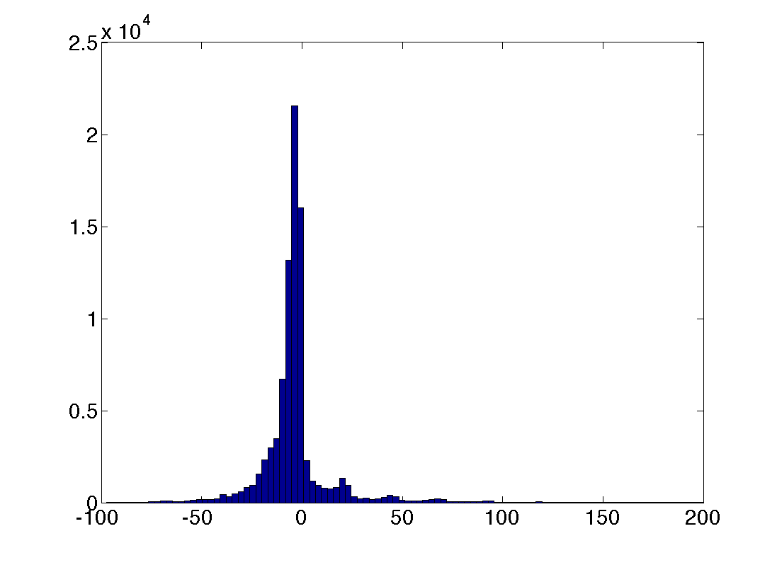
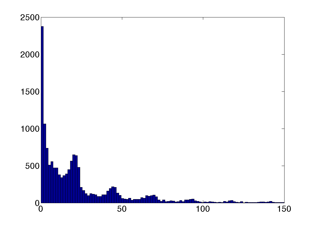
1. The left side of Figure 1 is the empirical distribution of transport risks of all shipments observed in the data (almost 90 thousand shipments), which, clearly, is a non-symmetric, long-tail distribution with several bumps at the distribution’s positive part. To better observe the bumps, we only plot the data that falls in the range $\left(0,\;150\right)$ on the right side of Figure 1. Here, we can see clearly that big bumps concentrate around days (at 24 hours, 48 hours, and 72 hours, etc.) and small bumps concentrate between days. These systematic peaks are largely due to the fact that a cargo that failed to be loaded onto its scheduled flight was loaded onto a flight on the same route later. The scheduled gap between flights, which depends heavily on the route, for example, is usually around 24 hours for international flights and several hours for domestic flights. The time gaps between scheduled flights thus transfer to the gaps between different peaks in the conditional distribution of transport risk to form a multimodal distribution; see ${\cal x}$3 for more detail.

Previous empirical studies primarily focus on domestic passenger flight arrival or departure delays; see Deshpande and Arikan (2012) for a review. Most of this literature assumes delays follow unimodal distributions, adopting linear models; e.g, Shumsky (1995) and Mueller and Chatterji (2002). However, delay distributions exhibit clear multimodality, making linear models unsuitable for air cargo transport risk assessment and prediction. The previous focus on linear models may have been due to the use of data from the US Department of Transportation (DOT) collected at the level of each flight. Our data are instead collected at the level of each cargo trip, including information on a trip from the beginning to end, usually consisting of several connecting flights. Data on the full trip allow us to explore new transport uncertainties not considered before. Specifically, we include information on delays due to missed flights within transportation risk. The clear multimodality in the full trip delay distributions motivates the new modeling approaches proposed in this paper. However, the modeling methods we develop are not restricted to cargo transport risk but can also be applied to other transport risks (e.g., passenger air transport). For an air passenger, the transport risk is determined by when the passenger arrives at the destination. Passenger arrival time can be different from the arrival time of the planned last flight since the passenger might miss the final flight due to a delay of his/her previous flight or some errands at the connecting airport. From this perspective, the passenger transport risk problem is similar to the cargo transport risk problem that we study in this paper.

To our best knowledge, the closest work to ours is Tu et al. (2008). The authors studied the departure push-back delay of flights using a model consisting of three parts accounting for seasonality, daily trends and a residual error modeled by a mixture distribution with Gaussian kernels and mixing weights fixed. The authors used the model to fit one year of data on flights originating from Denver International Airport and operated by United Airlines. However, the simplicity of their model makes it inapplicable to our study with much more volatile transport risks (as explain above) and also a much bigger data set containing cargo shipments to more than 200 airports operated by more than 20 airlines in 95 countries. To accommodate this complexity and better fit our data, we use a Bayesian nonparametric model. In extensive model comparisons with alternative models (see Appendix $\mathsection$B.5 for more details), including a flexible mixture model generalizing Tu et al. (2008), our model shows superior performance.

1.2 BNP Model and Conditional Distribution Function

Our second contribution is methodological. To accommodate the multimodal feature in the empirical transport risk distribution, we introduce a state-of-the-art Bayesian statistics tool – the BNP mixture model. To the best of our knowledge, no prior work has used related techniques in empirical OM, which so far predominantly applies frequentist statistics, such as ordinary least square estimation or maximum likelihood estimation, see, e.g., Deshpande and Arikan (2012), Li et al. (2014) and the references therein.

Bayesian statistics has experienced rapid development in the past two decades accelerated by ever-increasing computational power. Among these tools, BNP mixture models have become popular in the last several years, with applications in fields as diverse as finance, econometrics, genetics, and medicine (refer to Rodriguez and Dunson (2011) for references therein). A nonparametric mixture model can be expressed as follows: in the case where we are interested in estimating a single distribution from an independent and identically distributed ($i.i.d$) sample $y_{1},\cdots,y_{n}$, observations arise from a convolution

$$y_{j}\sim\int k\left(\cdot\mid\boldsymbol{\psi}\right)G\left(\mbox{d}\boldsymbol{\psi}\right)$$

where $k\left(\cdot\mid\boldsymbol{\psi}\right)$ is a given parametric kernel indexed by $\boldsymbol{\psi}$ (we use bold symbol to indicate vector), and $G$ is a mixing distribution assigned a discrete form

$$G\left(\boldsymbol{\psi}\right)=\sum_{l=1}^{L}\omega_{l}\delta_{\boldsymbol{\psi}_{l}},\;\mbox{where }\sum_{l=1}^{L}\omega_{l}=1\mbox{ and }\omega_{l}\geq 0,\;\forall l=1,\cdots,L$$

and $L$ can be finite or infinite. For example, assuming that $G$ follows a Dirichlet process prior leads to the well known Dirichlet process mixture model (Escobar and West 1995).

For our application, we adopt a specific BNP model — the PSBP mixture model, which was formally developed in Rodriguez and Dunson (2011). This method is known for its flexibility, generality, and importantly, computational tractability. In addition, PSBP leads to consistent estimation of any conditional density under weak regularity conditions as shown in Pati et al. (2013). Rodriguez et al. (2009) used this technique to create a nonparametric factor model to study genetic factors predictive of DNA damage and repair. Chung and Dunson (2009) applied this tool to develop a nonparametric variable selection framework. Our model is designed to capture the transport risk distribution characteristics in all ranges, covering both recurrent and disruption risks.

Particularly, we focus on modeling the conditional distribution of transport risks, within the PSBP framework. Modeling the conditional distribution allows us to investigate the relationship between transport risks and potential predictors, including airline, route, shipping time, cargo weight etc, based on which we can further explore ways to improve transport reliability. We will explain this in more details in ${\cal x}$3.1.

To demonstrate the value of PSBP, we compare our transportation risk estimation with that obtained from a naive linear model (see Equation (10) in Appendix $\mathsection$B.5.1 for details). We show that the two methods deliver dramatically different results. For instance, the naive linear model fails to capture the critical roles airlines play in transport service levels, and more importantly, underestimates disruption risks, which can result in insufficient risk management strategies. We further compare our model with two generalized and advanced alternative models: generalized additive models (GAM) (see Equation (11) in Appendix $\mathsection$B.5.3 for details) and flexible mixture models (see Equation (12) in Appendix $\mathsection$B.5.3 for details). Overall, our PSBP model shows a strong in-sample and out-of-sample predictive power but is relatively heavy in computation time. For the detailed model comparison, please refer to ${\cal x}$3.5 and Appendix $\mathsection$B.5.

1.3 Data-Driven Risk Assessment Tool

Our method suggests a powerful and general tool to help supply chain risk assessment, a topic that has not received the attention it deserves. In particular, while supply chain risk management is gaining increasing attention from both practitioners and academics, a recent McKinsey & Co. Global Survey of Business Executives shows that “nearly one-quarter of firms say their company doesn’t have formal risk assessment.” On the other hand, as articulated in Van Mieghem (2011), managing risk through operations contains 4 steps: 1. identification of hazards; 2. risk assessment; 3. tactical risk decisions; 4. implement strategic risk mitigation or hedging. These four steps must be executed and updated recurrently. Among the four steps, step 1 is more experience and context based, which typically involves information from anecdotal records or long experience with the specific business processes. Step 4 is more action-based, requiring detailed organizational design and information systems to carry out the hedging strategies developed in step 3. These two steps may not need quantitative methods. Steps 2 and 3, on the other hand, require rigorous analysis and quantification, and therefore call for analytical research. While most of the supply chain risk management literature focuses on the third step, which involves developing strategies for reducing the probabilities of negative events and/or their consequences should they occur, this paper focuses on step 2 – risk assessment.

Risk assessment involves estimation of two components: (a) risk likelihood, i.e., “the probability that an adverse event or hazard will occur” and (b) risk impact, i.e., “the consequences of the adverse event” (Van Mieghem 2011). The long-term expected risk is the integration of these two parts. Kleindorfer et al. (2003) assess risk impact (part (b)) of catastrophic chemical accidents using data collected by the Environmental Protection Agency. Kleindorfer and Saad (2005) presented a conceptual framework for risk assessment and risk mitigation for supply chains facing disruptions. Different from these studies, our work focuses on using statistical methods to accurately estimate the risk likelihood (part (a)), which calls for more advanced scientific computation and analysis tools. Correctly identifying hazards and assessing risk has important implications for the effectiveness of alternative management policies (Cohen and Kunreuther 2007). Our study shows that a careful risk assessment is critical to developing tailored services for customers (i.e., shippers) of different types and selecting service suppliers.

The transport risk studied in this paper resembles the random yield/capacity risks in manufacturing studied by many authors; see, e.g., Federgruen and Yang (2009), Wang et al. (2010). Also, transportation disruption risk is an important type or component of random supply disruption risks considered by Song and Zipkin (1996), Tomlin (2006), etc. While most of these authors focus on risk mitigation strategies assuming a particular risk distribution, such as a Bernoulli distribution for disruption risks, the Bayesian PSBP mixture model introduced here can be used to generate empirical random yield distributions and disruption probabilities, when data are available.

The reminder of the paper is organized as follows: in ${\cal x}$2, we give a brief introduction of the air cargo logistics industry and its challenges, the data we used for this study and the research questions we ask. In ${\cal x}$3, we describe approaches for model selection, we introduce the PSBP mixture model and the algorithm for posterior computation, and we compare our model with other models based on goodness of fit and predictive performance. In ${\cal x}$4 we explain the results. In ${\cal x}$5 we propose several applications of our model to design more efficient operational strategies. In ${\cal x}$6, we conclude the paper and discuss future directions. Appendix A contains data cleaning steps, and the tables and figures illustrating the data. Appendix B contains certain algorithm details, model implementation steps, model checking and comparison results. Appendix C contains estimation results and selected figures.

2 Industry Background, Data Source, and Research Questions

Though a crucial part of global operations, the air cargo industry is less known to the public because it operates behind the scenes. For this reason, in order to understand our model and analysis, it is necessity to provide a brief background of the industry, which also explains the initial motivation for the industry to develop a standardized Cargo 2000 process. Our data is Cargo 2000 standardized.

2.1 Service Chain Structure

First, we examine the shipping process. Typically, an air cargo transport involves four parties: shippers (e.g., manufacturers), freight forwarders (forwarders in short), carriers (i.e., airlines) and consignees (e.g., downstream manufacturers or distributors); see Figure

Figure 2: Cargo flows from the shipper to the forwarder; then from the forwarder to the airline; then from the airline to the same forwarder. In the end, the forwarder delivers the cargo to the consignee

2 for an illustration. These four parties form a chain structure, usually called the air transport supply chain. A shipper initiates a transaction by providing the forwarder company with “(1) origin/destination; (2) collection/delivery date; (3) shipment details (cargo pieces, weight and volume); (4) shipper/consignee information; (5) product/shipping service required”(IATA 2014a). Following their route map, the forwarder picks up cargoes from the shipper at the required time, consolidating cargoes sharing the same route if possible, and then sends cargoes to the selected airline at an origin airport. The airline takes charge of cargoes until arriving at the destination airport. An airline might use a direct flight or 2 – 3 connecting flights based on the route map. The forwarder accepts cargoes at the destination, and delivers them to consignees.

To simplify terms, we refer to both the shipper and the consignee as the “customers”. Customers use forwarders in 90% of air cargo shipments. A forwarder is a service provider for its customers, while it in turn uses airlines as service providers. Upon receiving a shipping request, a forwarder sends a booking request to several airlines, choosing the most economic one that satisfies the agreed upon timetable. Large forwarders typically reserve a certain percentage (e.g., 30%) of the total space on most airlines, including passenger and cargo airlines.

2.2 Cargo 2000 (C2K) Standards

To compete against integrators (service providers who arrange door-to-door transportation by combining mode(s) of transportation, such as DHL, UPS etc.), Cargo 2000 (C2K) was founded by a group of leading airlines and freight forwarder companies, “IATA Interest Group”, in 1997. This initiative was designed to enable industry-wide participants to “provide reliable and timely delivery shipments through the entire air transport supply chain” (C2K Master Operating Plan (MOP) Executive Summary(IATA 2014a)). Specifically, they developed a system of shipment planning and performance monitoring for air cargo which allows proactive and realtime event processing and control. Currently C2K is composed of more than 80 major airlines, forwarders, ground-handling agents, etc (see Figure 7.1 in Appendix for the current members of C2K). C2K Quality Management System is implemented with two different scopes: Airport-to-Airport (A2A) and Door-to-Door (D2D). In this paper, we focus on the A2A level shipments due to data constraints.

The following describes how C2K is used to create a shipping plan, and how airlines and forwarders monitor, control, intervene and repair each shipment in real-time.

2.2.1 Plan

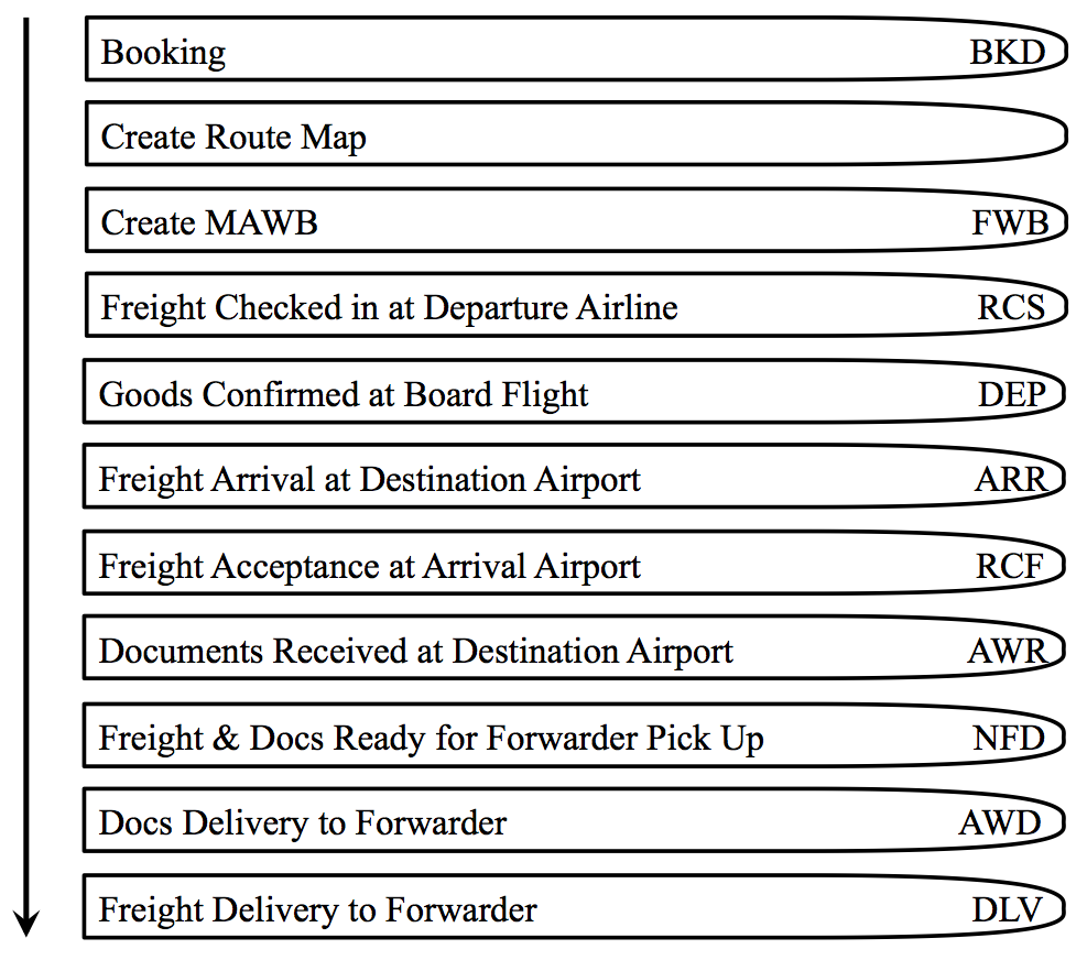
After a carrier has confirmed requested capacity on planned flights, it creates an A2A route map (RMP) and shares it with the forwarder. A RMP describes the path the shipment follows, including flight information, milestones and the latest-by time for the fulfillment of milestones along the transport chain. See Table A.1 and Figure 7.2 in Appendix ${\cal x}$A.2 for an illustration. If a customer agrees on the plan, the RMP is set alive. Otherwise, modifications will be made until agreement is achieved. Essentially, each route map is a combination of a station profile and milestones. Station profiles, which contain information on the duration for completion of each process step, are kept by forwarders and carriers. The milestones are defined by the C2K MOP.

2.2.2 Monitor, Control, Intervene and Repair

After a route map is issued, the shipping process is monitored against this map. The completion of every milestone triggers updates on both the airline’s and forwarder’s IT systems. Any deviation from the plan triggers an alarm, which allows for corrections to be taken by the responsible party in order to bring the shipment back on schedule. If necessary, a new RMP is made for the remaining transport steps. Meanwhile, an exception record is entered into the system recording the necessary information such as time, location, and reasons. See Table 7.2 in Appendix ${\cal x}$A.2 for an illustration.

2.2.3 Report

At the end of the shipment process, a report, including whether or not the delivery promise was kept and which party was accountable for the failure, is generated. This allows the customers to directly compare the performance of their C2K enabled forwarders, carriers and logistics providers.

2.3 Forwarder’s Frustration and Our Objectives

Even with current systems, the service level remains unsatisfying. As a result, forwarders risk loosing customers even though forwarders have no direct control of A2A, which is the most uncertain part of shipping. Questions for the forwarder to solve include: (1) how to predict transport risks so as to prepare for risks and inform customers in advance and (2) how to improve transport reliability in each route by selecting the best supplier? We aim to help address these questions. Suppose a customer comes to the forwarder with a fixed route (origin-destination), time of shipping, weight and volume of cargo. We aim to provide the forwarder with a distribution of transport risk conditional on demand variables (route, month, cargo weight/volume) and decision variables (airline, number of flight legs, planned duration, initial deviation time) with $95\%$ uncertainty interval. See Table

Table 1: Potential predictors

demand variables
route ($r$)	an origin-destination airport pair combination (captures all the fixed effects on a particular route).
month ($m$)	month when the shipping is finished
cargo weight ($wgt$)	total weight of the cargo (kilograms)
cargo number-of-pieces ($pcs$)	total number of pieces of the cargo (unit load)
decision variables
airline ($a$)	the airline transported the cargo
number of legs ($leg$)	number of connecting flights taken to arrival at destination
planned duration ($dur$)	total time (days) planned to take to finish the transport
initial deviation ($dev_{start}$)	deviation (days) between actual and planned check-in time at airline origin warehouse

1 for descriptions of these variables. Specifically, demand variables are determined by the shipper’s demand requirement which can not be changed. On the other hand, the decision variable can be chosen by the shipper at the time of purchasing shipping services. Based on this information, an optimal route can be chosen to match the customer’s cost/utility function, providing different options to different customers. Please refer to $\mathsection$5.1 for application illustration. Next, we elaborate how the above mentioned demand and decision variables affect the transport risk.

2.3.1 Effect of Demand Variables

1. Route: service level differs dramatically across routes depending on (a) supply-demand of air transport service and (b) congestion level and infrastructure at visited airports. We use a route-level effect to absorb all these factors.

2. Month: demand (e.g., holiday shipping) and weather (e.g., winter snow) both have a seasonal trend, which results in different perceived air cargo transport service levels in different months. We used the month, in which each shipment completes, as the predictor. Since shipments only take 1.7 days to complete on average, essentially identical results would be achieved using the month of transport start.

3. Cargo weight and volume: each flight has a maximum weight and volume (cargo volume is approximated by cargo pieces in this paper). Larger cargoes may be more likely to fail to be loaded onto the scheduled flight due to (1) airlines overselling capacities and (2) changes of currently available capacity, such as more luggage from passengers. However, larger cargoes are usually more valuable, thus may have higher transport priority.

2.3.2 Effect of Decision Variables

1. Airline: transportation delays are expected to vary substantially across airlines due to a wide variety of factors, and hence we added (1) the interaction of airline and route and (2) the interaction of airline and number of legs into the model.

2. Number of legs: number of legs increases the probability for a cargo to miss connecting flights, so it is a strong predictor of transport risk.

3. Planned duration: even conditional on route, airline and number of legs, planned duration differs greatly. This reflects cushions added to the shipping time.

4. Initial deviation: if the cargo is sent to the airline earlier than scheduled, it can be loaded onto an earlier flight and otherwise the cargo might miss it’s planned flight. Before the trip starts, the forwarder can use 0 as the default value to make transport risk prediction. As soon as the forwarder has sent the cargos to the airline, a new prediction can be made with the new time information.

2.3.3 Other Potential Predictors

There are other factors, such as price and weather, that may also affect the risk distribution, but are not available in our data. Our model indirectly captures these effects through allowing the distribution of risk to vary flexibly with the demand and decision variables mentioned above. Different definitions of demand/decision variables can be adopted, such as to replace our “route” with “path” (with connecting airports information). This can potentially improve the predictive accuracy. However since our data is sparse and our major focus is to present fundamental modeling details, we choose to retain our current settings while these specifics can be easily modified in our model.

2.4 Data and Summary Statistics

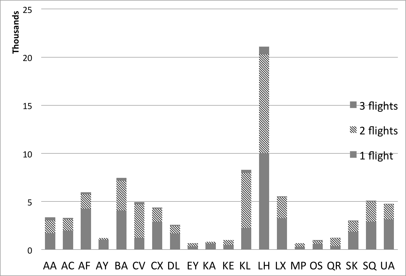
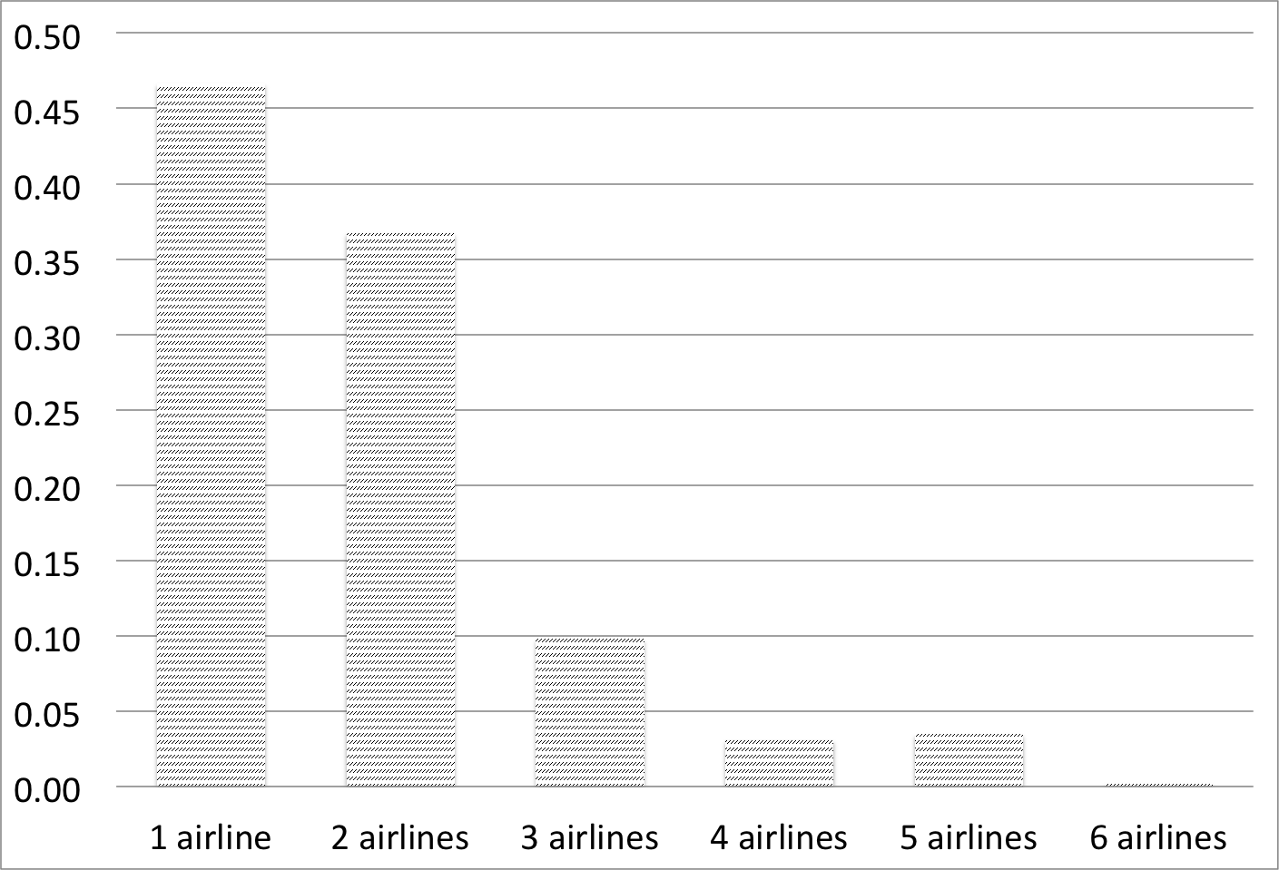
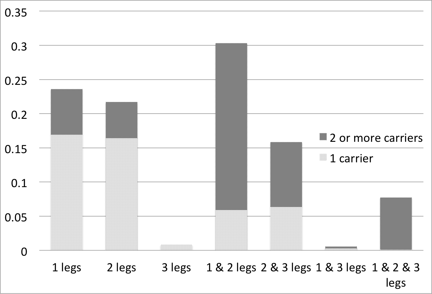
Our data contain a leading freight forwarder company’s C2K standard air freight shipments from October 2012 to April 2013. The data contain real-time milestone updates, similar to the data shown in Table A.1 in Appendix $\mathsection$A.2, and route maps for each shipment. The last route map before the shipment is used to measure risk. After cleaning (see Appendix ${\cal x}$A.1 for cleaning steps), the data include 86,149 shipments on 1336 routes operated by 20 airlines. Freights are shipped from 58 countries to 95 countries. In Appendix ${\cal x}$A.3 are summary statistics. In sum, we observe that: (i) European airlines, such as Lufthansa and KLM, play a significant role in the data; (ii) More than 50% of shipments are transported on routes served by more than 1 airline. For example, around 30% of shipments are on routes served both by direct flights and 2-leg service; (iii) There are more than 50% of shipments transported on routes where services of different legs are available. This confirms the need for a careful assessment of the impact of different choices, which can lead to a higher utility if service levels vary significantly.

3 Model

In this section, we explain the model in details. ${\cal x}$3.1 provides motivation for estimating the conditional distribution of transport risk and advantages of using the PSBP mixture model. The model can be decomposed into two parts: mixture weight and mixture kernel, detailed in ${\cal x}$3.2 and ${\cal x}$3.3, respectively. The Bayesian posterior sampling algorithm to estimate unknown parameters in weights and kernels is presented in ${\cal x}$3.4. We also discuss model selection and comparison in ${\cal x}3.5$. Detailed supplementary materials can be found in Appendix ${\cal x}$B.

3.1 Conditional Risk Distribution

Figure 3: True data (histogram), PSBP predictive (solid curve) and naive linear model predictive (dashed curve) mean conditional response density $\hat{f}(y\mid{\bf x})$. Left: route = Frankfurt to Shanghai, airline = KLM; Right: route = London to Atlanta, airline = Delta. For the exact method to calculate predictive conditional response density, please refer to ${\cal x}$5.2.

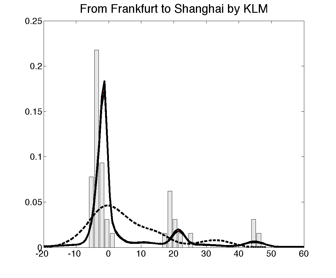
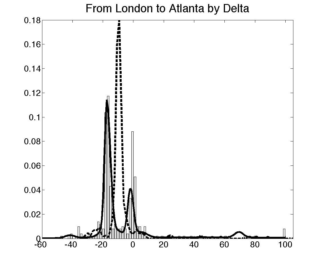
The multimodal feature is not only present at the aggregate data level, see Figure 1, but also at the granular level, such as each route or route-airline level. The histograms in Figure 3 show the empirical distributions on two sample routes served by two airlines. In order to make accurate predictions and inferences based on such data, the first step is to choose a model flexible enough to fit the data well. Usual choices of models for multimodal data rely on mixtures, e.g., mixtures of Normal kernels, which are known to provide an accurate approximation to any unknown density.

We cannot rely on simple mixture models, as we are investigating the distribution of transport risks conditional on demand and decision variables, including both categorical and continuous predictors. This leads to a problem of conditional distribution estimation. One stream of literature on flexible conditional distribution estimation uses frequentist methods. Fan et al. (1996) proposed a double-kernel local linear approach, and related frequentist methods have been considered by Hall et al. (1999) and Hyndman and Yao (2002) among others. The other popular choice is a BNP mixture model. Muller et al. (1996) proposed a Bayesian approach to nonlinear regression, in which the authors modeled the joint distribution of dependent variable and independent variables using a Dirichlet process mixture of Normals (Lo 1984, Escobar and West 1995). This type of approach induces a model for the conditional distribution of the response through a joint model for the response and predictors. Although such joint models are provably flexible, in practice they can have clear disadvantages relative to models that directly target the conditional response distribution without needing to model the high-dimensional nuisance parameter corresponding to the joint density of the predictors. Such disadvantages include treating the independent variables as random, while they are often designed variables (e.g., it seems unnatural to consider route or airline as random), and relatively poor practical performance in estimating the conditional distribution.

We instead focus on direct modeling of the unknown conditional distribution of transport risk $y$ given predictors ${\bf x}=\left(x_{1},\cdots,x_{p}\right)^{{}^{\prime}}\in{\cal X}$ (${\cal X}$ is the sample space for the predictors ${\bf x}$) without specifying a model for the marginal of ${\bf x}$. In our context, predictors ${\bf x}$ = {airline $\left(a\right)$, route $\left(r\right)$, month $\left(m\right)$, number of legs $\left(leg\right)$, initial deviation $\left(dev_{start}\right)$, planned duration $\left(dur\right)$, cargo weight $\left(wgt\right)$, cargo number of pieces $\left(pcs\right)$} (as specified in Table 1). In particular, we assume the transport risk $y$ arises from a convolution

$$y\mid{\bf x}\sim\int k\left(y\mid\boldsymbol{\psi}\right)G_{{\bf x}}\left(\mbox{d}\boldsymbol{\psi}\right)$$ (1)

where $k\left(\cdot\mid\boldsymbol{\psi}\right)$ is a given parametric kernel indexed by parameters $\boldsymbol{\psi}$ (e.g., Normal kernel $k\left(\cdot\mid\boldsymbol{\psi}\right)$ is indexed by $\boldsymbol{\psi}=$(mean, standard deviation)), and the mixing distribution $G_{{\bf x}}$ is allowed to vary flexibly with predictors ${\bf x}\in{\cal X}$. The typical form in the BNP literature (refer to Rodriguez and Dunson (2011) for references) lets

$$G_{{\bf x}}=\sum_{l=1}^{L}\omega_{l}\left({\bf x}\right)\delta_{\boldsymbol{\psi}_{l}\left({\bf x}\right)},\mbox{ where }\sum_{l=1}^{L}\omega_{l}\left({\bf x}\right)=1\mbox{ and }\omega_{l}\left(x\right)\geq 0$$ (2)

where the atoms $\left\{\boldsymbol{\psi}_{l}\left({\bf x}\right):{\bf x}\in{\cal X}\right\}_{l=1}^{L}$ are $i.i.d$ sample paths from a stochastic process over ${\cal X}$, and $\left\{\omega_{l}\left({\bf x}\right),{\bf x}\in{\cal X}\right\}$ are predictor-dependent probability weights that sum to one for all $x$. The above form is too general to be useful and it is necessary to make some simplifications for practical implementation. One common possibility is to introduce predictor dependence only in the $G_{{\bf x}}$ atoms, $\psi_{l}\left(x\right)$, while keeping weights, $\omega_{l}\left({\bf x}\right)=\omega_{l}$, fixed. However, this approach tends to have relatively poor performance in our experience, including the air cargo transport risk data, we have also shown this in model comparison with Flexmix model (see Appendix $\mathsection$B.5.3 for details).

In our case, the peak locations of the dependent variable, transport risk, are almost constant (i.e., daily peaks for international shipments, and some additional few-hourly peaks for domestic shipments besides the daily peaks). However, the heights of the peaks change greatly along with ${\bf x}$ (e.g., route, airline, demand variables). The height of each peak represents (roughly) the probability for the observation to fall into the kernel centered around that peak. For example, if conditional on certain ${\bf x}_{1}$, the peak around 24 hours is relatively high, then a shipment, conditional on ${\bf x}_{1}$, has a large probability of being delayed for 24 hours. On the other hand, if conditional on certain ${\bf x}_{2},$ there is only one significant peak around 0 hours, then a shipment, conditional on ${\bf x}_{2}$, probably arrives close to the planned arrival time. So, in our context, to find out how the height of each peak depends on ${\bf x}$ is of central interest.

Inducing dependence structure in the weights can be difficult and lead to complex and inefficient computational algorithms, limiting the applicability of the models. To overcome these difficulties, we adopt the PSBP mixture model, which has the advantages of computational tractability and consistency under weak regularity conditions.

3.2 Bayesian Probit Stick-breaking Process

Recalling the general form of the mixing measure in Equation (2), stick-breaking weights are defined as $\omega_{l}=u_{l}\prod_{p<l}\left(1-u_{p}\right)$, where the stick-breaking ratios are independently distributed $u_{l}\sim H_{l}$ for $l<L$ and $u_{L}=1$ for the case of finite $L$. In the baseline case in which there is no predictor, Probit stick-breaking weights are constructed as

$$u_{l}=\Phi\left(\gamma_{l}\right),\;\gamma_{l}\sim\mathsf{N}\left(\mu,\phi\right)$$

where $\Phi\left(\cdot\right)$ denotes the cumulative distribution function (cdf) for the standard normal distribution. $\mu$ is the mean and $\phi$ is the precision (the reciprocal of the variance) of a normal distribution such that for $x\sim\mathsf{N}\left(\mu,\phi\right)$, the probability density function (pdf) is $f(x)=\sqrt{\frac{\phi}{2\pi}}\exp\left\{-\frac{\phi}{2}\left(x-\mu\right)^{2}\right\}$. For a finite $L$, the construction of the weights ensures that $\sum_{l=1}^{L}\omega_{l}=1$. When $L=\infty$, $\sum_{l=1}^{\infty}\omega_{l}=1$ almost surely (Rodriguez and Dunson 2011).

The use of Probit transformation to define the weights builds a mapping between a real number $\gamma_{l}$ from $-\infty$ to $+\infty$ into $u_{l}\in(0,1)$. Thus, the transformation allows researchers to restate the model using normally distributed latent variables $\gamma_{l}$, facilitating computation via data augmentation Gibbs sampling algorithms presented in $\mathsection$3.4. This transformation also makes model extensions to include additional structure (e.g,. predictors) straightforward. Additionally, the Probit transformation simplifies prior elicitation as presented at the end of ${\cal x}3.2$.

In order to make $\omega_{l}\left({\bf x}\right)$ predictor-dependent, we further express the latent variables $\gamma_{l}$ as a linear function of ${\bf x}$, $\left\{\gamma_{l}\left({\bf x}\right),{\bf x}\in{\cal X}\right\}$ (In this paper we use superscript as an index rather than the exponent of the parameter):

$$\omega_{l}\left({\bf x}\right) = \Phi\left(\gamma_{l}\left({\bf x}\right)\right)\prod_{p<l}\left(1-\Phi\left(\gamma_{p}\left({\bf x}\right)\right)\right)$$ (3)

$$\gamma_{l}({\bf x}) = \theta_{l}^{1}+\theta_{a}^{2}+\theta_{r}^{3}+\theta_{\left(a,r\right)}^{4}+\theta_{m}^{5}+\theta_{leg}^{6}+\theta_{\left(a,leg\right)}^{7}+f_{1}\left(dev_{start}\mid\boldsymbol{\theta}^{8}\right)$$ (4)

$$+f_{2}\left(dur\mid\boldsymbol{\theta}^{9}\right)+f_{3}\left(\mbox{log}\left(wgt\right)\mid\boldsymbol{\theta}^{10}\right)+f_{4}\left(\mbox{log}\left(pcs\right)\mid\boldsymbol{\theta}^{11}\right)$$

where $\{\theta_{l}^{1}\}$ controls the baseline probability of latent class $l$ ($l=1,\cdots,L$), $\{\theta_{a}^{2}\}$ controls the baseline heterogeneity of airline $a$ ($a=1,\cdots,20$), $\{\theta_{r}^{3}\}$ controls the heterogeneity of route $r$ ($r=1,\cdots 1336$), $\left\{\theta_{\left(a,r\right)}^{4}\right\}$ represents the dependence of weights on possible interactions between airlines and routes, and the meanings of $\left\{\theta_{m}^{5}\right\}$, $\left\{\theta_{leg}^{6}\right\}$,$\left\{\theta_{\left(a,leg\right)}^{7}\right\}$ are similar. In addition, $f_{1}$, $f_{2}$, $f_{3}$ and $f_{4}$ are spline functions expressed as a linear combination of B-splines of degree 4 (see Appendix $\mathsection$B.4 for details of the smooth splines used), where the knots of $dev_{start}$ are [-3, -2, -1, 0, 1, 2, 3], the knots of $dur$ are [1, 2, 4, 6, 8, 10], the knots of $log(weight)$ are [2, 4, 6, 8] and the knots of $log(pcs)$ are [1, 3, 5]. Here we use the logarithm form of cargo weight $\left(wgt\right)$ and number of pieces $\left(pcs\right)$ as the predictors, since the original distributions are highly skewed. To ensure identification of the parameters, we let $\theta_{1}^{2}=\theta_{1}^{3}=\theta_{\left(1,r\right)}^{4}=\theta_{\left(a,1\right)}^{4}=\theta_{1}^{5}=\theta_{(1,leg)}^{6}=\theta_{(a,1)}^{7}=0$ for all $a$, $r$ and interactions in sample space ${\cal X}$.

3.3 Posterior Computation

In Bayesian statistics, the posterior distribution is typically not available analytically, involving an intractable normalizing constant. For this reason, posterior calculations usually rely on either large sample approximations, which may have questionable accuracy in our transportation risk applications, or Markov chain Monte Carlo (MCMC) sampling. The basic idea in MCMC sampling is to construct a Markov chain having stationary distribution corresponding to the joint posterior distribution of the model parameters, with this done in a manner that avoids ever having to calculate the intractable constant. In order for the Markov chain to have the appropriate behavior, the Markov transition kernel needs to be carefully chosen, with usual choices corresponding to either Metropolis-Hastings (MH) or Gibbs sampling. MH can involve a lot of tuning in models with many parameters, while Gibbs avoids tuning by sampling sequentially from the conditional posterior distributions of subsets of parameters given current values of the other parameters. Gibbs sampling relies on a property known as conditional conjugacy. Focusing on a subset of the model parameters and conditioning on the other parameters, the prior probability distribution is conditionally conjugate if the conditional posterior distribution takes the same form as the prior. The specific choices of our model form and prior distributions (to be described below) are motivated by retaining conditional conjugacy.

In order to obtain conditional conjugacy for blocks of parameters, we follow a common strategy known as data augmentation. The basic idea in data augmentation is that one may obtain conditional conjugacy, and hence a simple Gibbs sampling algorithm, by introducing latent variables in a careful manner. The MCMC algorithm is then run for both the latent variables and the model parameters; although this increases the number of unknowns to sample, it can lead to greater efficiency by allowing model parameters to be sampled in blocks directly from full conditional posterior distributions. Similar augmentation strategies are routinely used in frequentist statistics; e.g., to fix mixture models with the EM algorithm. Here, we follow the augmentation strategy of (Rodriguez et al. 2009). First we focus on case when $L<\infty$. For each observation $y_{j}\mid{\bf x}$, (corresponding to replicate $j$ conditional on ${\bf x}$, $j=1,\cdots,n\left({\bf x}\right)$ if there are $n({\bf x})$ replicates, otherwise $j$ is dropped if there are no replicates, i.e., $n({\bf x})=1$), we introduce a latent indicator variable $s_{j}\left({\bf x}\right)$ such that $s_{j}\left({\bf x}\right)=l$ if and only if observation $y_{j}\mid{\bf x}$ is sampled from mixture component $l$ ($l=1,2,\cdots,L$). The use of these latent variables is standard in mixture models. With the help of latent indicators $s_{j}({\bf x})$, Gibbs sampling of more than 2000 model parameters can be classified into four categories, as presented in Appendix $\mathsection$B.1.1 $\sim$ $\mathsection$B.1.5.

3.4 Distributional Choices

To complete a specification of our model, we require a specific choice for the kernel in the kernel mixture, as well as prior probability distributions for each of the model parameters. These choices are described below.

3.4.1 Normal Kernel

A mixture of a moderate number of Normals is known to produce an accurate approximation of any smooth density. Also motivated by computational tractability of the Normal distribution (i.e., conditional conjugacy), we specify the parametric kernel, $k\left(\cdot\mid\boldsymbol{\psi}\right)$, of the PSBP mixture model as a Normal distribution, $\mathsf{N}\left(\mu,\phi\right)$, where $\boldsymbol{\psi}=\left(\mu,\phi\right)$. Recalling that our mixture model takes the form in Equation (1), we replace the kernel in the above equation with Normal and use the PSBP specified prior $G_{{\bf x}}$. Then the conditional distribution of $y$ can be expressed in the simple form

$$y\mid{\bf x}=\sum_{l=1}^{L}\omega_{l}\left({\bf x}\right)\mathsf{N}\left(y\mid\mu_{l},\phi_{l}\right)$$ (5)

The prior of atoms $\left\{\left(\mu_{l},\phi_{l}\right),l=1,2,\cdots,L\right\}$ is $\mathsf{N}\mathsf{G}(\zeta_{\mu},\xi_{\mu},a_{\phi},b_{\phi})$, a conditionally-conjugate Normal-Gamma prior such that

$$\mu_{l}\sim\mathsf{N}\left(\zeta_{\mu},\xi_{\mu}\phi_{l}\right), \phi_{l}\sim\mathsf{G}\left(a_{\phi},b_{\phi}\right).$$

where $l=1,2,\cdots,L$. The specification of prior $\zeta_{\mu},\xi_{\mu},a_{\phi}$ and $b_{\phi}$ is discussed in Appendix ${\cal x}$B.2.

3.4.2 Prior for Parameters in Weight

We choose Normal priors for parameters $\Theta=${$\left\{\theta_{l}^{1}\right\}$, $\left\{\theta_{a}^{2}\right\}$, $\left\{\theta_{r}^{3}\right\}$, $\left\{\theta_{\left(a,r\right)}^{4}\right\}$, $\left\{\theta_{m}^{5}\right\}$, $\left\{\theta_{leg}^{6}\right\}$, $\left\{\theta_{\left(a,leg\right)}^{7}\right\}$, $\boldsymbol{\theta}^{8}$, $\boldsymbol{\theta}^{9}$, $\boldsymbol{\theta}^{10}$, $\boldsymbol{\theta}^{11}$}

$$\theta_{j}^{i}\sim\mathsf{N}\left(\nu^{i},\epsilon^{i}\right),\mbox{ for }i=8,\cdots,11\mbox{ and }j=1,\cdots,n(i)$$

where $n(i)$ is the number of B-spline basis used for predictor $i$. For the coefficients of 7 categorical independent variables $\boldsymbol{\theta}^{1},\cdots,\boldsymbol{\theta}^{7}$ (i.e., $\boldsymbol{\theta}^{1}=\left\{\theta_{l}^{1}\right\}$ etc), we build a hierarchy, which enables information borrowing among parameters in one category

$$\theta_{l}^{1}\sim\mathsf{N}\left(\Phi^{-1}\left(\frac{1}{L-l+1}\right),\epsilon^{1}\right), \theta_{a}^{2}\sim\mathsf{N}\left(0,\epsilon^{2}\right),\cdots \theta_{\left(a,leg\right)}^{7}\sim\mathsf{N}\left(0,\epsilon^{7}\right).$$

where $\epsilon^{i}\sim\mathsf{G}\left(c_{i},d_{i}\right)$ for $i=1,2,\cdots,7$. Here $\mathsf{G}(a,b)$ is a Gamma distribution such that for $x\sim\mathsf{G}(a,b)$ the pdf is $f(x)=\frac{b^{a}}{\Gamma\left(a\right)}x^{a-1}e^{-bx}$. We use the specially designed prior of $\theta_{l}^{1}$ to enforce the same prior baseline probability of each cluster $l=1,2,\cdots,L$. The specification of $\left\{\left(c_{i},d_{i}\right),\mbox{ for }i=1,2,\cdots,7\right\}$ and $\left\{\left(\nu^{i},\epsilon^{i}\right),i=8,9,\cdots,12\right\}$ is discussed in Appendix ${\cal x}$B.2.

3.5 Model Fitting Assessment

In order to select a specific set of predictors to include in our PSBP mixture model, we rely on comparing different possibilities using cross validation. In particular, we select a model having the best out-of-sample predictive performance. Details are provided in Appendix ${\cal x}$B.4, and the selected model is shown in Equation (6). This model is used for later model comparison and application illustration.

$$\gamma_{l}({\bf x}) = \theta_{l}^{1}+\theta_{a}^{2}+\theta_{r}^{3}+\theta_{\left(a,r\right)}^{4}+\theta_{m}^{5}+\theta_{leg}^{6}+f_{1}\left(dev_{start}\mid\boldsymbol{\theta}^{8}\right)+f_{2}\left(dur\mid\boldsymbol{\theta}^{9}\right)+f_{3}\left(\mbox{log}\left(wgt\right)\mid\boldsymbol{\theta}^{10}\right)$$ (6)

It is important to assess how well this model fits the data, while verifying that it does not overfit. In general, Bayesian methods are protected against overfitting due to the implicit penalty on model complexity that appears in the posterior distribution but not in maximum likelihood estimation. In mixture models, overfitting can occur by using too many mixture components. However, the PSBP mixture model and related Bayesian nonparametric models automatically favor placing all but a negligible amount of the probability weight on a few components. This is consistent with our observation of superior out-of-sample predictive performance relative to flexible frequentist regression models.

We follow a common Bayesian strategy of goodness of fit checking by using posterior predictive plots. In particular, the basic idea is to generate new data from the posterior predictive distribution under our PSBP mixture model and see how the observed data relate to these model generated data. If the model fits poorly, a systematic deviation will show up. We observe an excellent goodness of fit based on these assessments. On the contrary, a naive linear model, shown in Equation (10) in Appendix $\mathsection$B.5, shows extremely poor fit. We additionally compare our model with frequentist generalized additive models (GAMs) and flexible mixture models using both in-sample and out-of-sample prediction residuals. Overall, our model presents a superior performance. For interested readers, please refer to Appendix ${\cal x}$B.5 for more details.

4 Results

Table 9.1 in Appendix ${\cal x}$C.1 shows the posterior mean and 95% probability interval of (selected) model parameters. There are several things to note from the table:

1. The 50 kernel means, $\mu_{1},\mu_{2},\cdots,\mu_{50}$, range from -70.0 to 77.5 (hours), indicating the model predicted deviation concentrates within -3 to 3 days, consistent with the data. The 50 kernel standard deviations, $1/\sqrt{\phi_{1}},1/\sqrt{\phi_{2}},\cdots,1/\sqrt{\phi_{50}}$, range from 0.62 to 84.4, meaning the Normal kernels can be very narrow or flat, allowing for flexible estimation.

2. Level parameters, $\theta_{1}^{1},\theta_{2}^{1},\cdots,\theta_{49}^{2}$, vary from -10.9 to 6.74, and the wide range suggests strong variation in risk. For example, if an airline-route pair has $\gamma_{l}\left({\bf x}\right)-\theta_{l}^{1}$ close to zero, then for certain $l$ with $\theta_{l}^{1}$ smaller than -5, the weight $\propto$ $\Phi\left(\gamma_{l}\left({\bf x}\right)\right)$ $\approx$ $\Phi\left(-5\right)$ $\approx$ 0, thus eliminating the inclusion of this component. By similar arguments, $\theta_{l}^{1}$ can also help determine for which $\gamma_{l}\left({\bf x}\right)-\theta_{l}^{1}$ component $l$ plays major role.

3. The posterior distributions of all the coefficients are substantially more concentrated than their prior distributions, suggesting that the data provide substantial information to update the priors; in addition, the 95% probability intervals are narrow.

4. The posterior estimation of airline coefficient (we disguise the names of airlines for confidentiality reasons. The airline index used here is randomly assigned), $\theta_{a}^{2}$, shows great heterogeneity, and the large standard deviation, $1/\sqrt{\epsilon^{2}}$, which measures the variations among airlines, confirms this from one other aspect. Closer inspection reveals that except A1, whose coefficient is fixed at zero for identification, 18 of the remaining 19 airlines’ 95% probability intervals don’t include 0. Furthermore, many of them are far from zero, implying large impact on transport risk. However, based on the linear model (see Equation (10) in Appendix $\mathsection$B.5), only 2 of the 19 airlines are significantly different from 0 at 5% confidence level. This huge difference underlies the principle of the two estimation methods. The naive linear model focuses in estimating the effects of independent variables on distribution mean, and its results indicate airlines don’t necessarily affect the mean of transport risk much. However, PSBP’s results show that airlines are playing an important role on selecting and weighting possible kernels, which affects the tail shape, number of peaks, probability of extreme observation etc. These results and comparison once again show that the linear model, which cannot detect the airlines’ (and some other predictors’ including routes’ etc) impact on transport risk in this case, would lose considerable valuable information.

5. Since the number of routes and their interactions with airline are large, 1336 and 587 respectively, we don’t include their posterior summaries in Table 9.1. However, posterior summaries of hyper-parameters standard deviation, $1/\sqrt{\epsilon^{3}}$, illustrate the large heterogeneity between routes. More importantly, the large standard deviation, $1/\sqrt{\epsilon^{4}}$, represents possibly huge differences in terms of the distribution of transport risks on the same route while by different airlines. This suggests that a careful selection of carriers can result in dramatically different shipping experiences.

5 Applications

Estimates of predictive conditional probability density functions (Cpdfs) are key to generating data-driven operation strategies. In this section, we provide several examples of how posterior Cpdfs can aid decision making. We note that there are other applications of our transport risk models.

5.1 Service Comparison for One Shipment

The most straightforward use of PSBP posterior estimation is to provide predictive Cpdf of transport risk to shippers based on their predetermined demand variables and selectable decision variables (see Table 1). This not only helps the shipper to find a preferable service but also helps the forwarder to set a price quote. Assume a customer comes with predetermined demand requirement $d=\left\{r,m,wgt\right\}$ and is choosing from services $s=\left(a,leg,dur\right)\in S\left(d\right)$, where $S\left(d\right)$ is the set of services available given demand factors, $d$. Here, even though the initial deviation, $dev_{start}$, is one of the decision variables, we set it to 0 because this variable is unknown and not selectable before shipping starts. Let $f\left(risk\mid d,s\right)$ be the predictive distribution of transport risk conditional on $d$ and a chosen $s$, and $l_{i}\left(risk\right)$ be customer $i$’s loss function. The optimal conditional choice of $s$, which minimizes expected transport loss, is defined as

$$\left(s\mid d\right)_{i}^{*} \triangleq \mbox{argmin}_{s\in S\left(c\right)}Loss_{i}\left(s\mid d\right)$$

$$Loss_{i}\left(s\mid d\right) = \int l_{i}\left(risk\right)f\left(risk\mid d,s\right)\mbox{d}dev$$ (7)

where $Loss_{i}\left(s\mid d\right)$ is customer $i$’s expected loss of choosing $s$ given $d$. Estimating each customer’s unknown loss function $l_{i}\left(dev\right)$ is another interesting study of practical value, but is outside the scope of this paper. Here we use several generic loss functions to illustrate how to use predicted $f\left(risk\mid d,s\right)$ to aid service selection.

In Figure

Figure 4: PSBP predictive (solid curve) conditional response density $\hat{f}\left(y\mid x\right)$ with 95% credible interval (dotted curve) of the normal (bottom) and speedy (top) services from three airlines A6 (left), A8 (middle) and A13 (right) on the route from Frankfurt (Germany) to Atlanta (United States). For details of the calculation method, please refer to ${\cal x}$5.2.

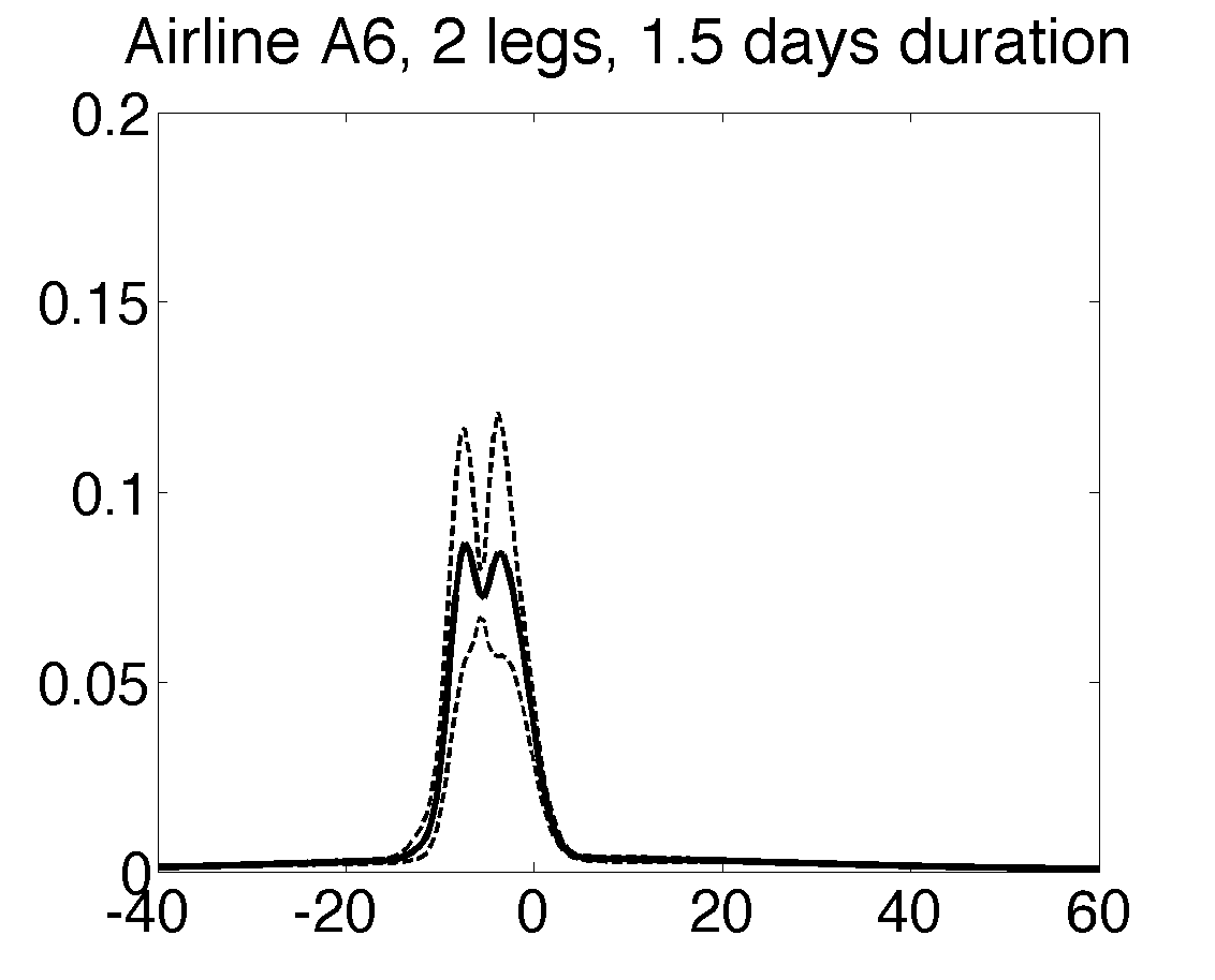
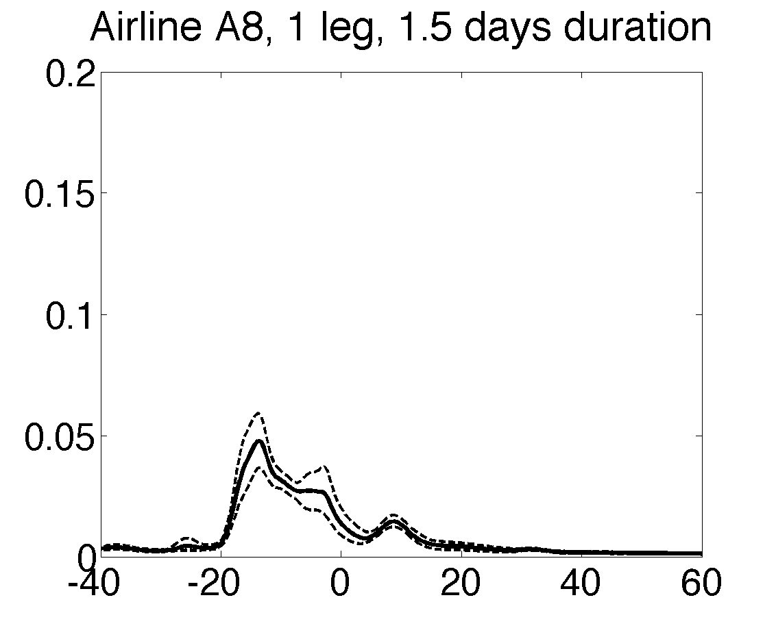
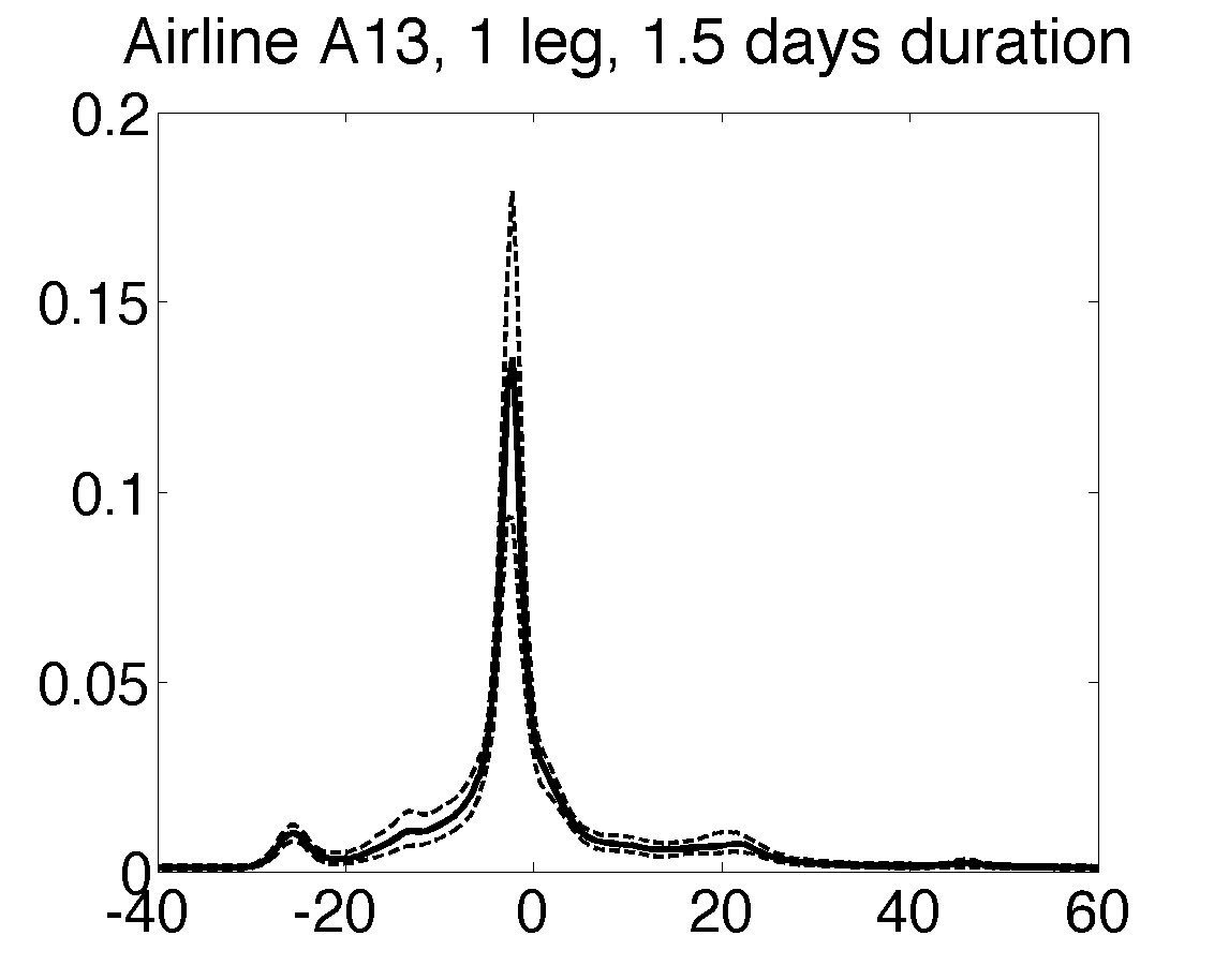
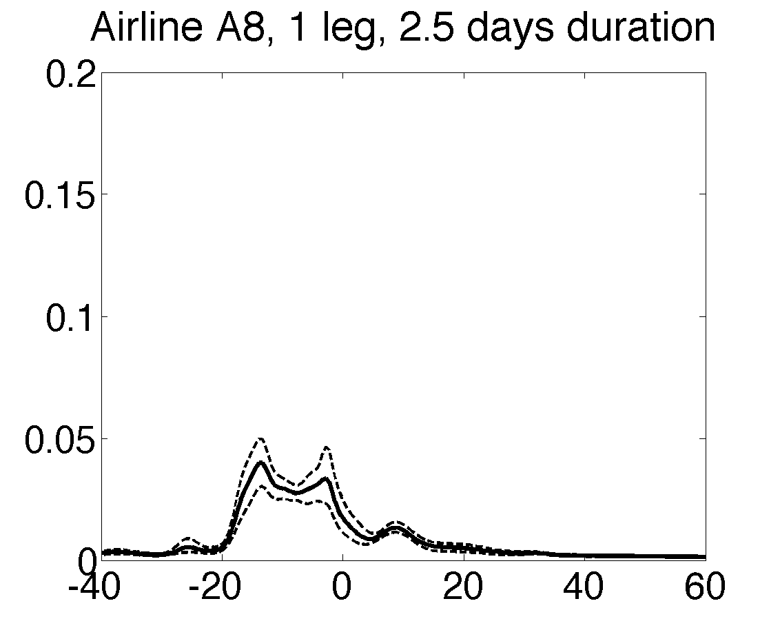
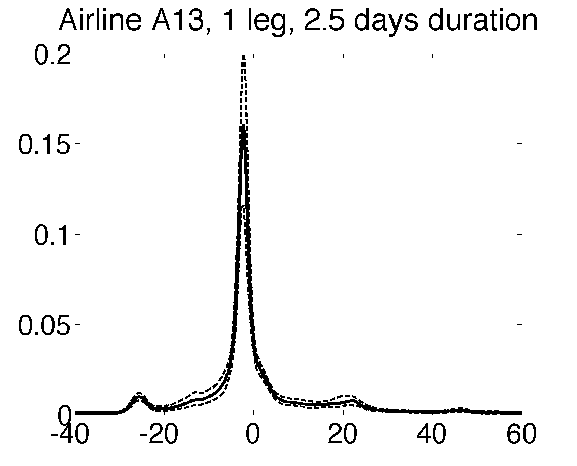
4 are 6 choices as shown by the figure titles, on the route from Frankfurt to Atlanta. The choices are randomly picked from the data. We use the following three loss functions:

$$l_{1}\left(risk\right)=C_{1}\cdot risk l_{2}\left(risk\right)=C_{2}\cdot{\bf 1}\left\{risk>18\right\} l_{3}(risk)=C_{3}\cdot risk^{2}$$

$l_{1}$ naturally arises when a risk neutral shipper is adverse to delays while fond of early arrivals; $l_{2}$ is more proper when a shipper is sensitive to extreme delays exceeding certain threshold (18 hours in our example); $l_{3}$ is used when a shipper is risk adverse and dislikes any deviations from the plan, neither negative nor positive. Under these loss functions, the expected losses have simple analytical forms

$$Loss_{1}=C_{1}\cdot\mathsf{E}_{f} Loss_{2}=C_{2}\cdot\left(1-F\left(18\right)\right) Loss_{3}=C_{3}\cdot\left(\mathsf{Var}_{f}+\mathsf{E}_{f}^{2}\right)$$

where $f$ is short for $f\left(risk\mid d,s\right)$ and $F$ is the corresponding cumulative density function. Figure

Figure 5: Expected loss (with 95% credible interval) of the normal and speedy services from three airlines A6, A8 and A13 on the route from Frankfurt (Germany) to Atlanta (United States). Left: $Loss_{1}=C_{1}\cdot\mathsf{E}_{f}$; Middle: $Loss_{2}=C_{2}\cdot\left(1-F\left(18\right)\right)$; Right: $Loss_{3}=C_{3}\cdot\left(\mathsf{Var}_{f}+\mathsf{E}_{f}^{2}\right)$

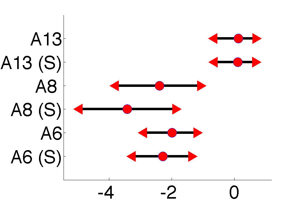
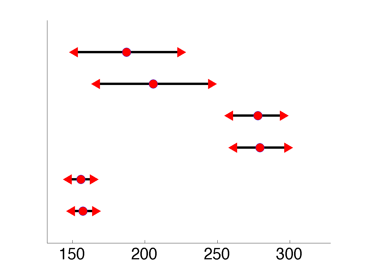
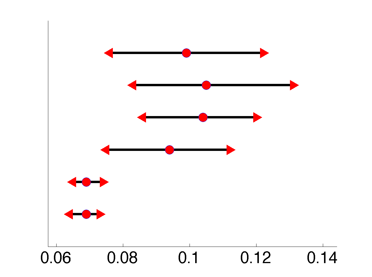
5 presents the expected losses (with posterior 95% probability intervals) calculated for the six choices under 3 risk functions with $C_{1}=C_{2}=C_{3}=1$, in which we use (S) to indicate $speedy$ service. We observe (1) the rank of services in terms of expected loss varies by loss functions; (2) choice of airlines is playing a more dominant role than the choice between normal and speedy services given an airline.

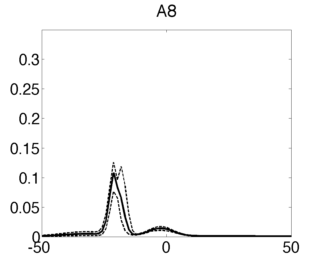
With estimated expected loss of each choice, forwarders can offer different price quotes to different types of shippers. In this example, a forwarder can increase revenue by lowering A8’s prices to attract price-sensitive shippers and increasing A6’s prices to attract quality-sensitive shippers under loss function 2.

5.2 Supplier Ranking on Route or Higher Level

Unlike a shipper, whose decision is made at the level of each shipment, a forwarder plans its business at the route or higher level. To help solve problems at high levels, the full predictive Cpdf should be integrated. Specifically, let the full information set be $U=${$a$, $r$, $m$, $leg$, $dur$, $dev_{start}$, $wgt$}, for $U=U_{1}\cup U_{2}$ and $U_{1}\cap U_{2}=\phi$, then

$$f\left(risk\mid U_{1}\right)=\int f\left(y\mid U_{1},U_{2}\right)f\left(U_{2}\right)dU_{2}$$

where $U_{1}$ contains variables of central interest, and other variables in $U_{2}$ are integrated out. For example, a practical problem faced by a forwarder is whether to choose a carrier on a certain route and how much capacity to reserve from it. For such decisions, an estimation of the airline’s service reliability is a critical input. In this case airlines and routes are of interest, so we let $U_{1}=\left\{a,r\right\}$ and $U_{2}=U-U_{1}$. By using Equation (7) with $c$ and $s$ replaced by $r$ and $a$, the forwarder can obtain expected losses by each airline $a\in S\left(r\right)$, which, in turn, can help make the right capacity reservation and pricing decisions.

5.3 Baseline Comparison

Our result can also be used to generate baseline comparisons of various factors. Baseline effect of a certain factor excludes the effects of any other factors, thus allowing for a direct comparison between factors of one type.

Figure 6: Reference performances of sample airlines A2 (left), A9 (middle) and A13 (right) with predictive density mean (solid curve) and 95% credible interval (dotted curve)

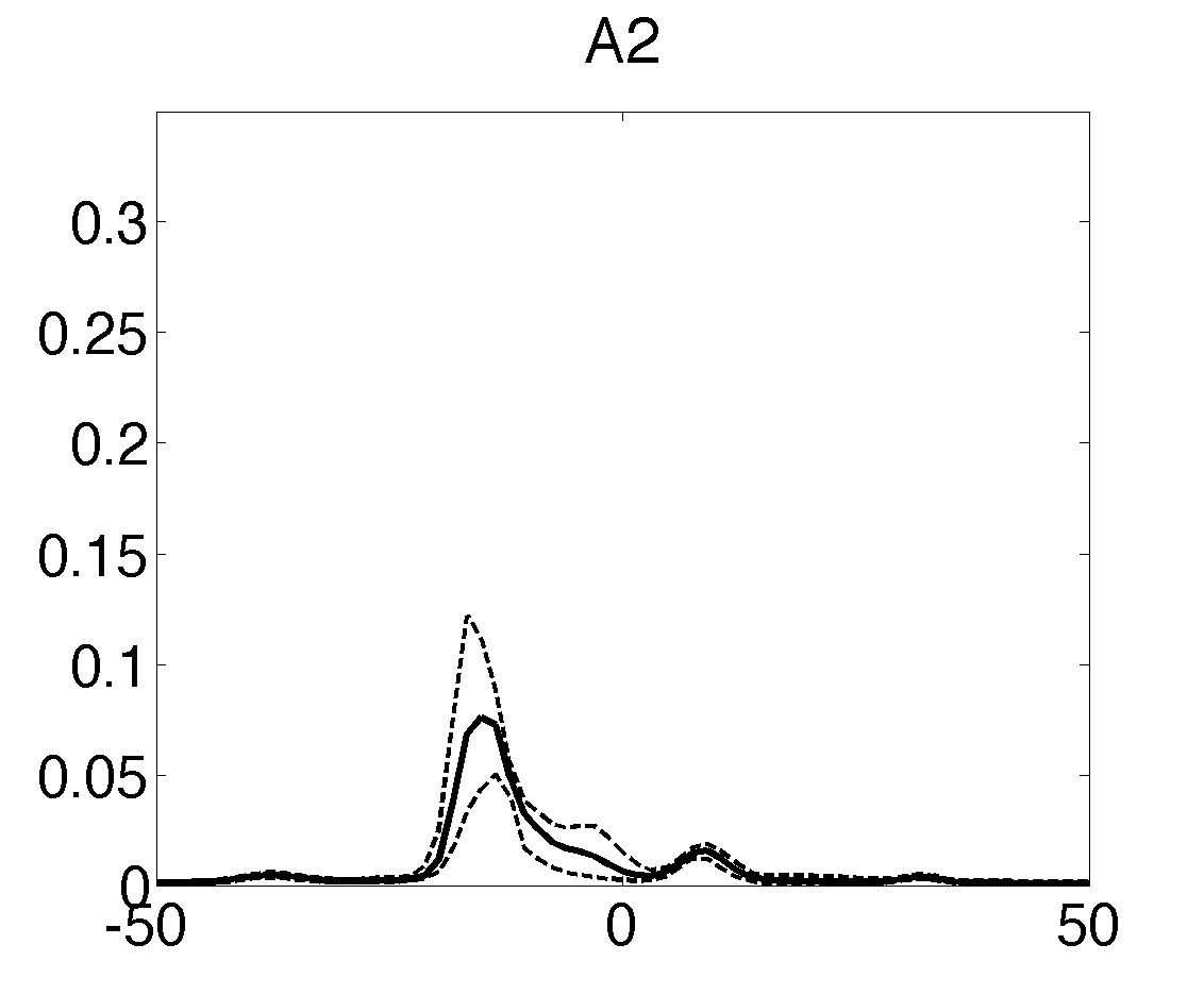
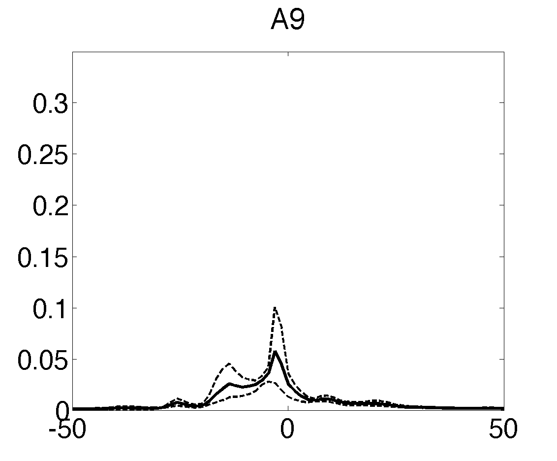
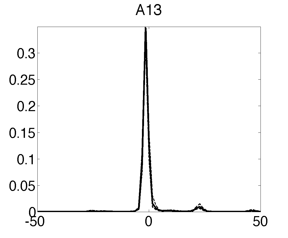
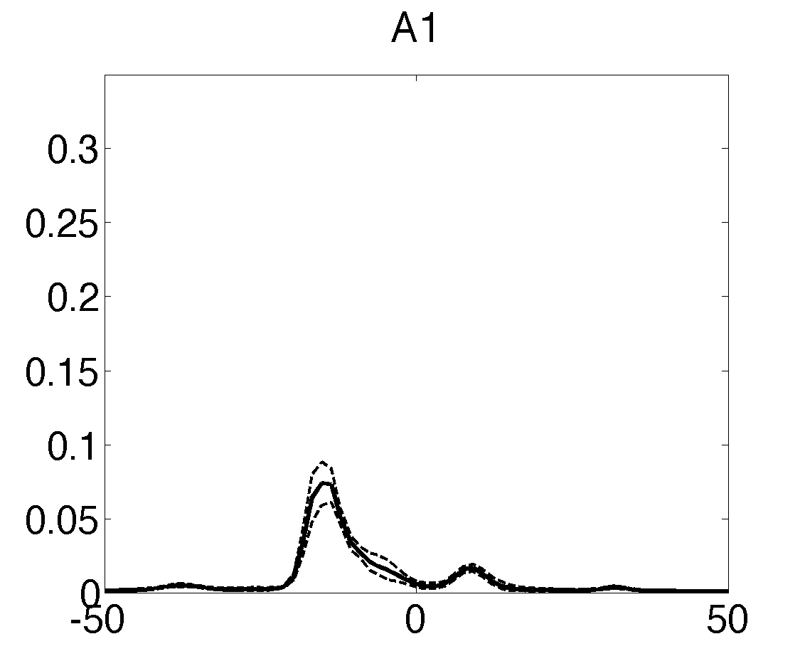
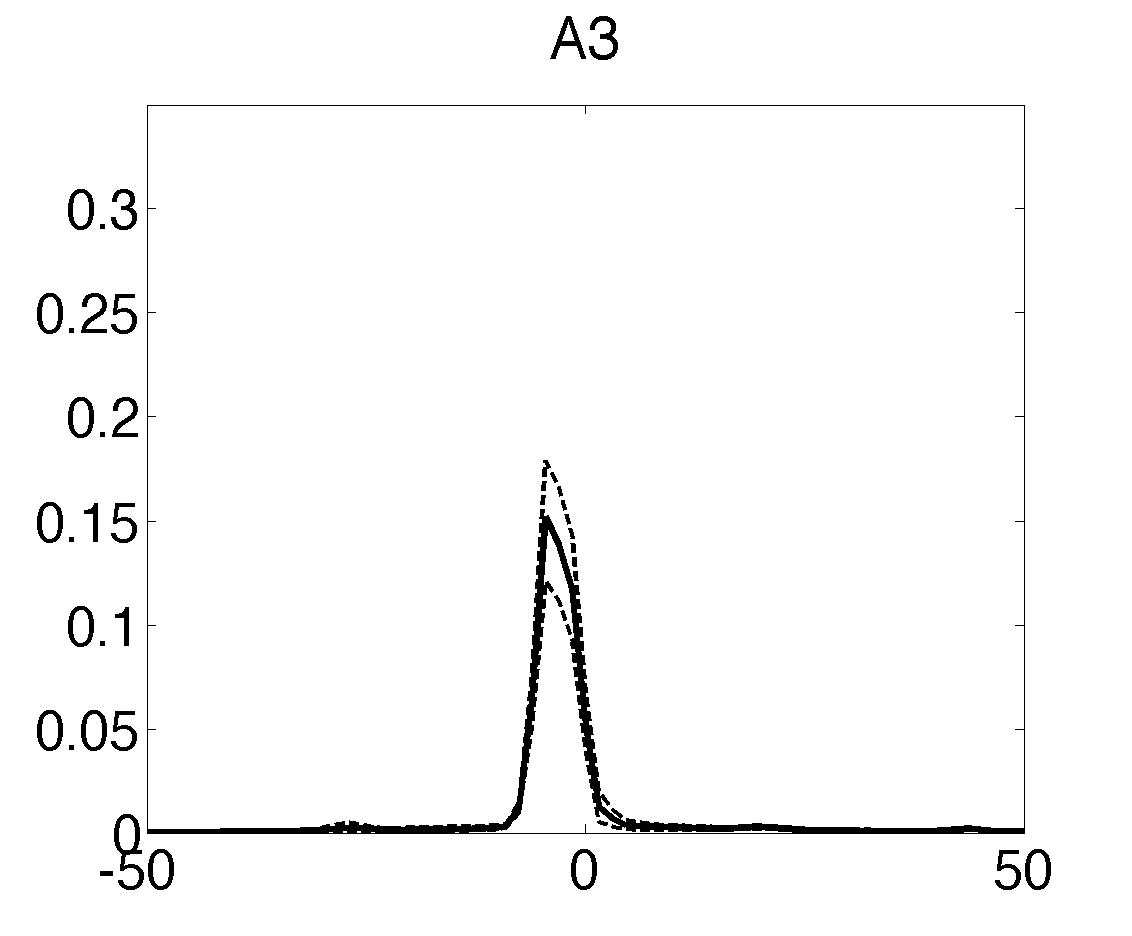
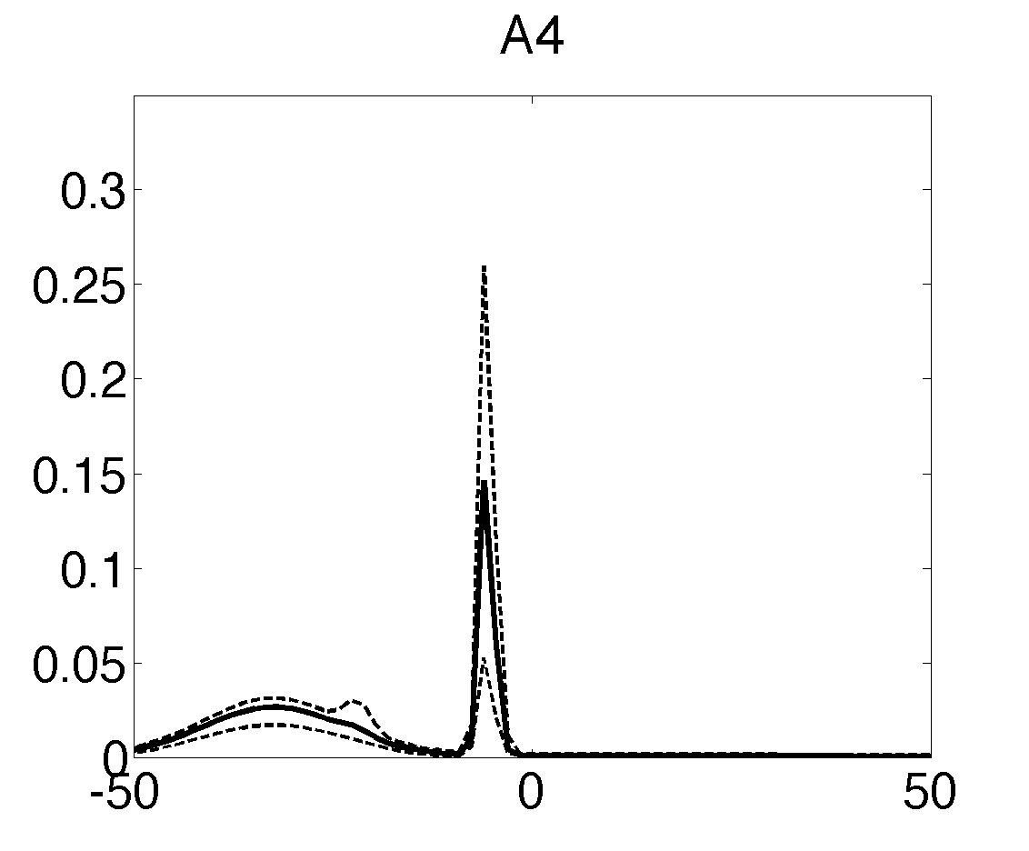
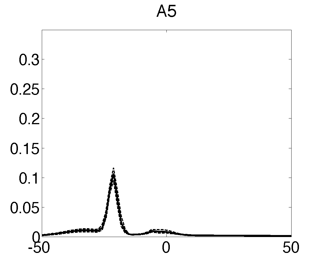
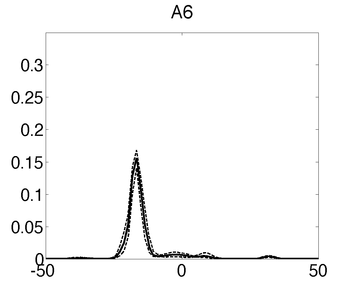
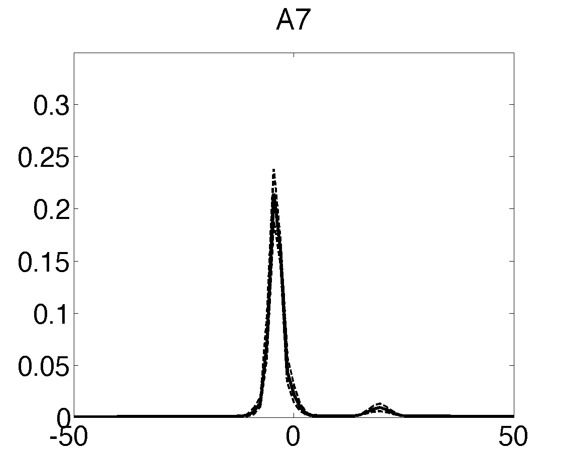
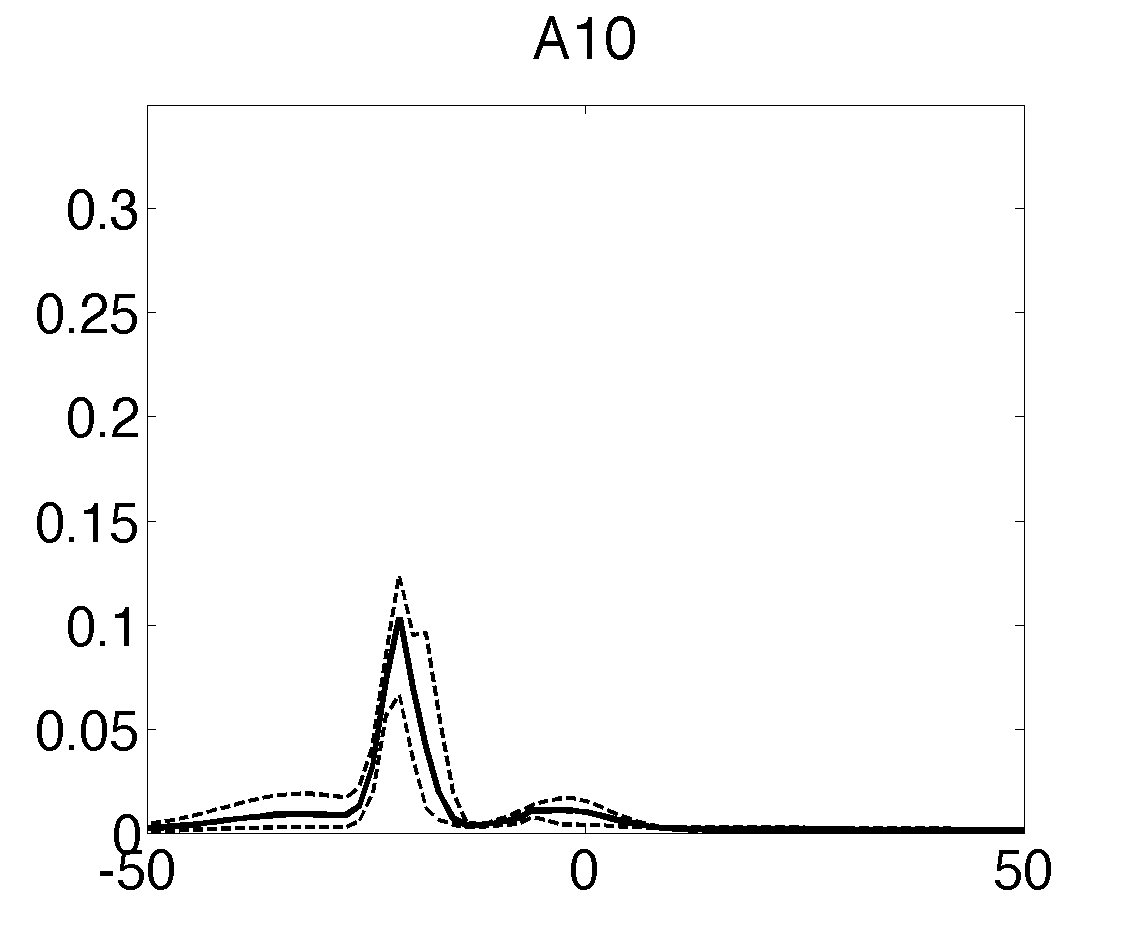
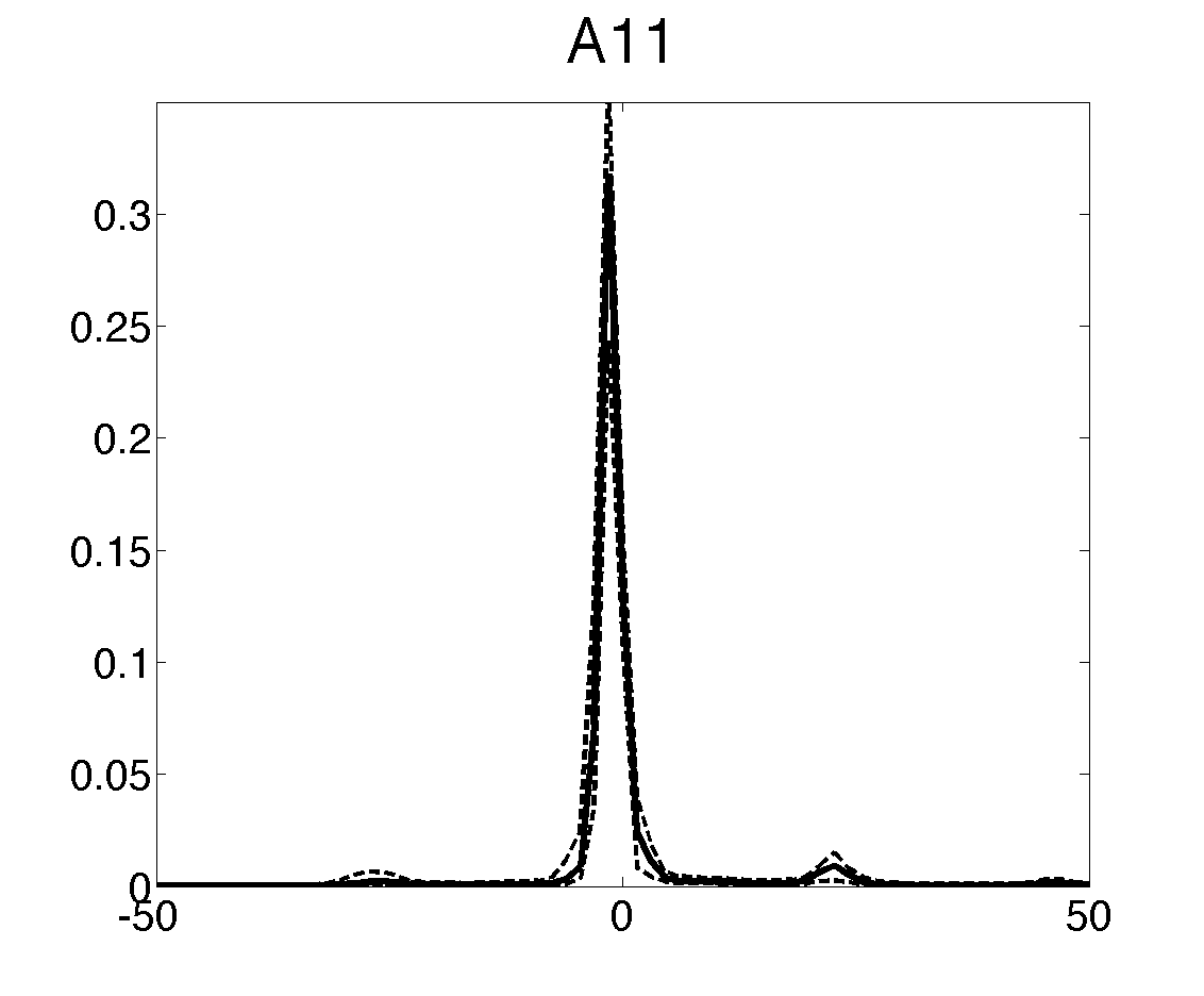
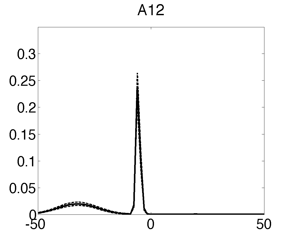
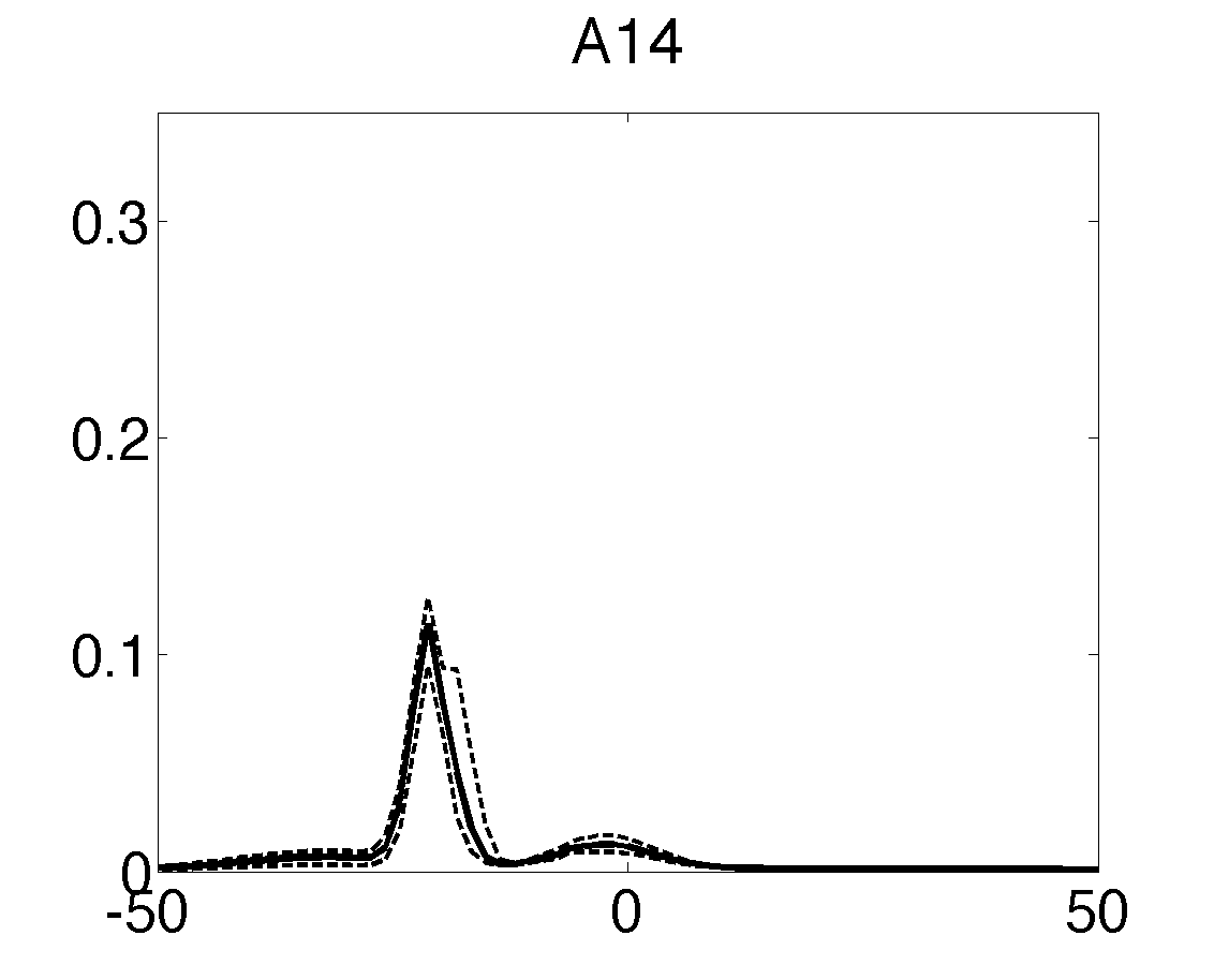
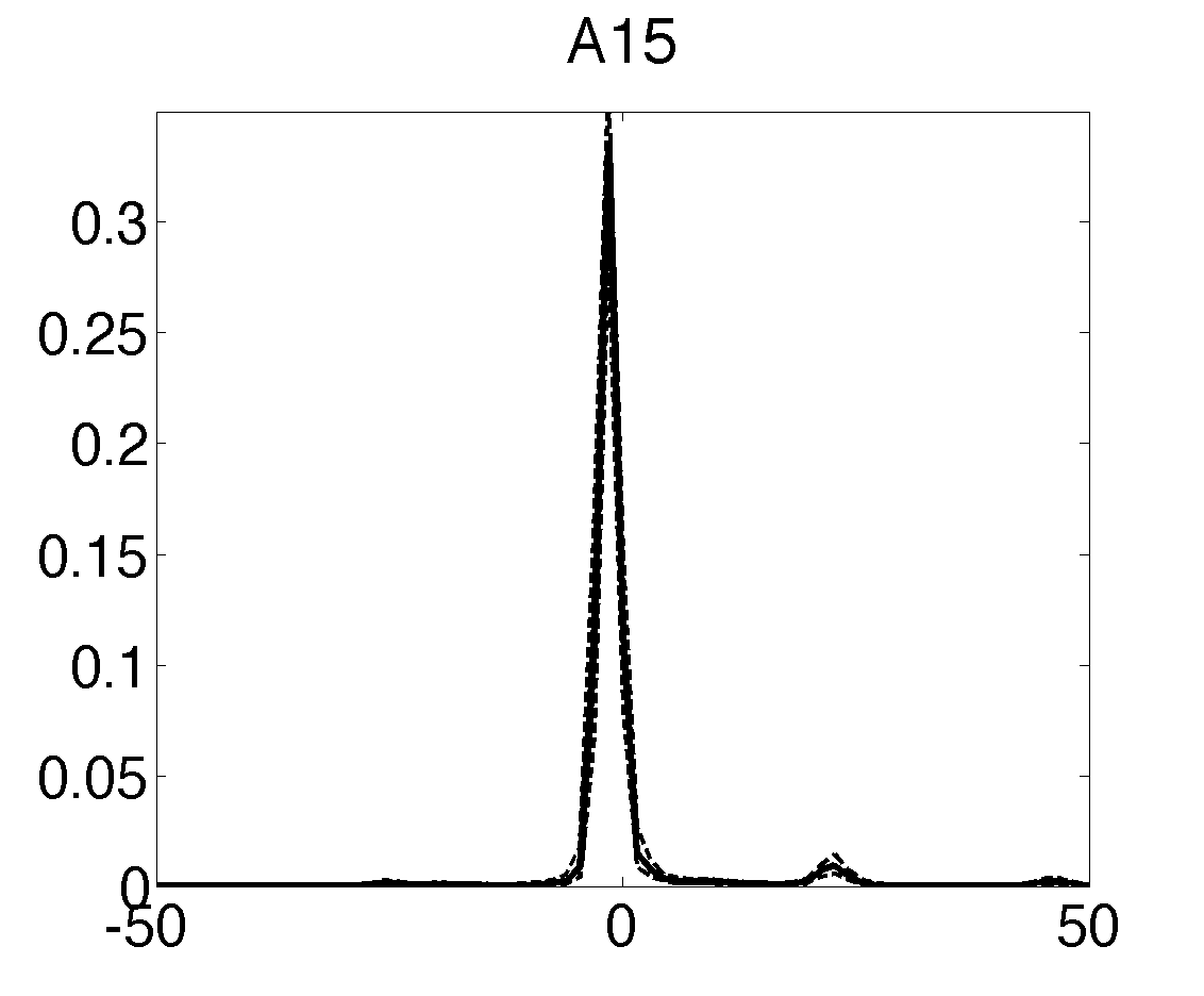
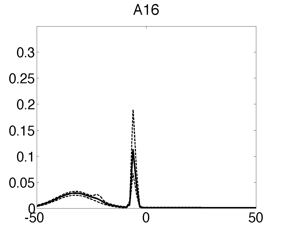
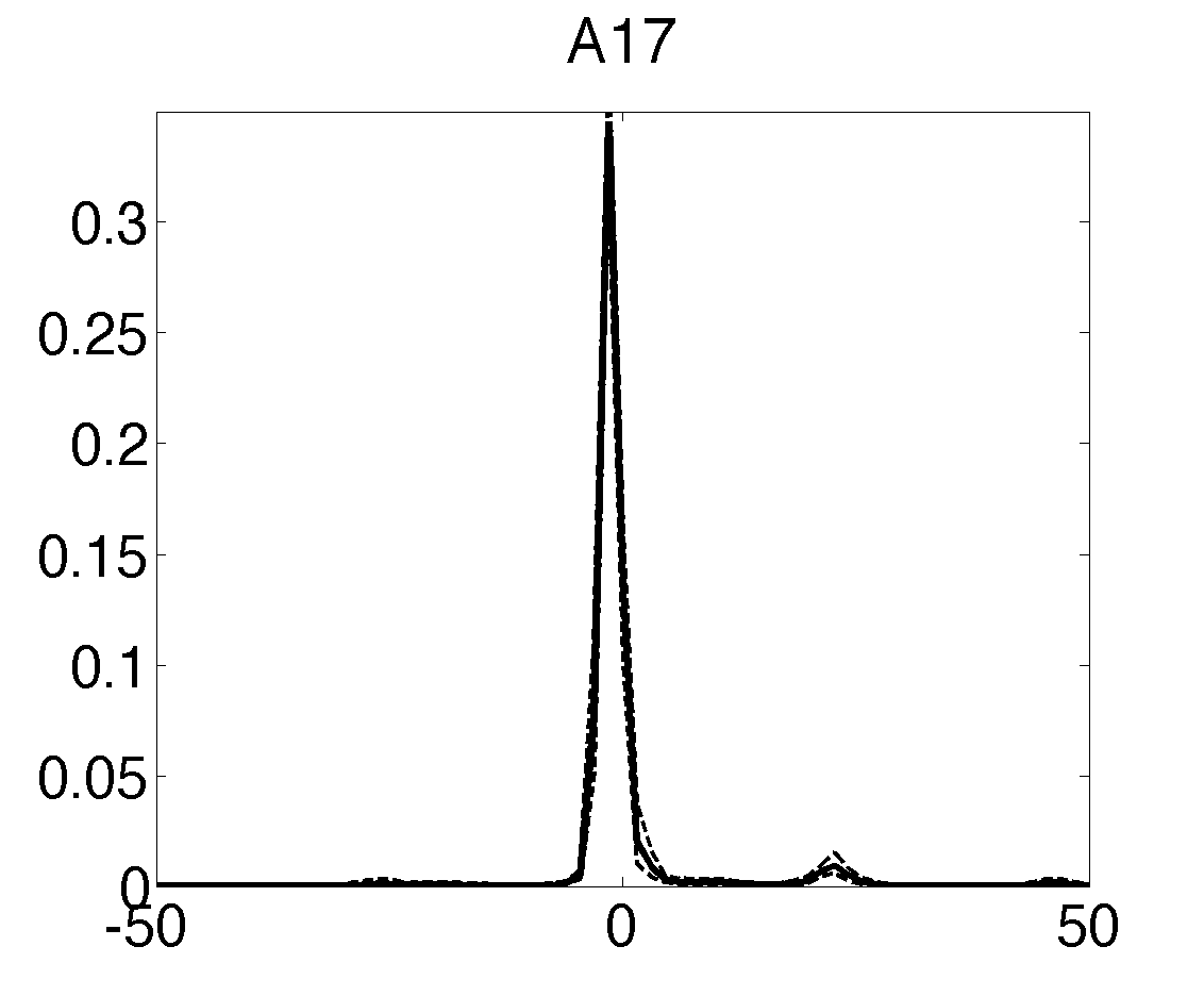
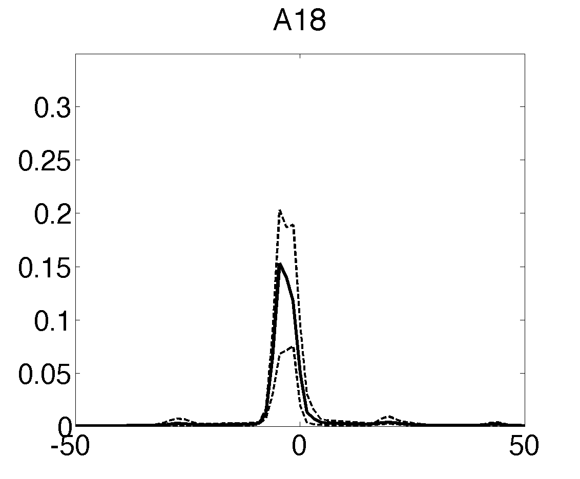
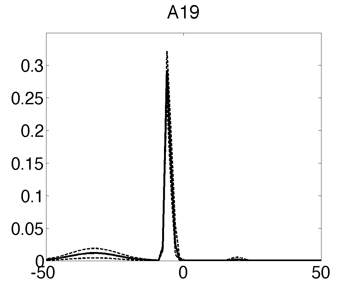
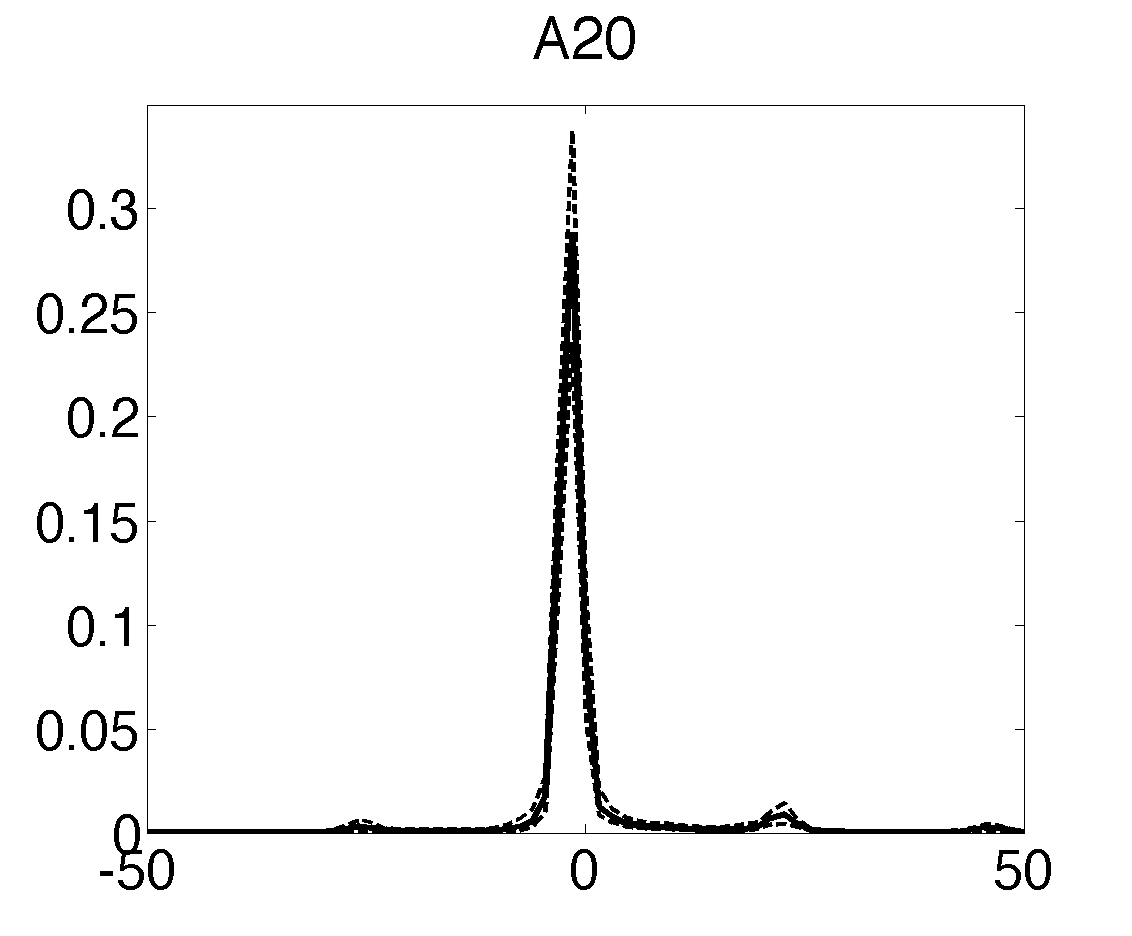
One interesting example is to understand the baseline performance of each airline, in which case a direct comparison is impossible due to the fact that airlines serve different routes. To achieve this baseline comparison, we use the average value for all other predictors, except airline effects $\theta_{a}^{2}$, as their reference levels. Then we plug these reference levels in the posterior samples of each airline and then obtain the reference risk distribution for each airline (See Figure 6 for 3 samples from the 20 airlines. See Appendix ${\cal x}$C.2 for the remaining 17 baseline distributions). From the plots we can directly compare airlines, which differ from each other by the number, locations, and heights of peaks. As such, our model allows baseline comparison based on distribution knowledge. This offers a much richer comparison than those appearing in the literature based on single average metrics. Meanwhile, the richer tool allows us to obtain simple metric comparisons as special cases.

For example, using a U.S. passenger flight data set, Deshpande and Arikan (2012) analyzed single-leg flight truncated block time, which is transport risk plus planned duration minus initial deviation. Initial deviation is defined as the positive delay of the previous flight by the same craft if applicable and zero otherwise. The authors argue that if the truncated block time is shorter than the scheduled block time, the airline incurs an overage cost of $C_{o}$ per unit overage time. Otherwise, the airline incurs an underage cost $C_{u}$ per unit shortage time. The authors then estimate the overage to underage ratio, $\varphi=C_{0}/C_{u}$, for each flight, and calculate the mean ratio of flights served by a certain airline as the airline-wise overage to underage ratio, $\varphi_{a}$. Using our international air cargo data, we can obtain an analogous metric by replacing “schedule block time” and “truncated block time” in their paper with $dur$ and $\left(dur+\mbox{arrival deviation}-[dev_{start}]^{+}\right)$. One concern of estimating airline-wise ratio $\varphi_{a}$ by simply calculating the average of flight-wise ratios is that the effects from other factors, such as routes etc, cannot be excluded. Thus, the calculated overage to underage ratio of each airline, $\varphi_{a}$, cannot be used for direct comparison of airlines’ intrinsic service quality. Baseline distribution of airlines, on the other hand, is a good solution to this problem. Specifically, the optimal $dur^{*}$ is defined by news-vendor solution that

$$\mathsf{Prob}\left(dur^{*}+\mbox{arrival deviation}-\left[dev_{start}\right]^{+}\leq dur^{*}\mid a\right) = \frac{1}{1+\varphi_{a}}$$

$$\mathsf{Prob}\left(\mbox{arrival deviation}\leq 0\mid a\right) = \frac{1}{1+\varphi_{a}}$$ (8)

where we use the fact that the reference level of $\left[dev_{start}\right]^{+}$, calculated by the data average, is zero. Thus each airline’s overage to underage ratio is calculated by $\varphi_{a}=\frac{1}{F_{a}\left(0\right)}-1$

Figure 7: For each of the 20 airlines in the data: the red dot in the center of the arrow is the mean overage to underage ratio calculated by PSBP; the arrow represents the 95% posterior probability interval; the blue circle is the overage to underage ratio from the C2K Monthly Statement issued by IATA (if there is no overage to underage ratio reported in the C2K monthly statement, the blue circle is missing for that airline).

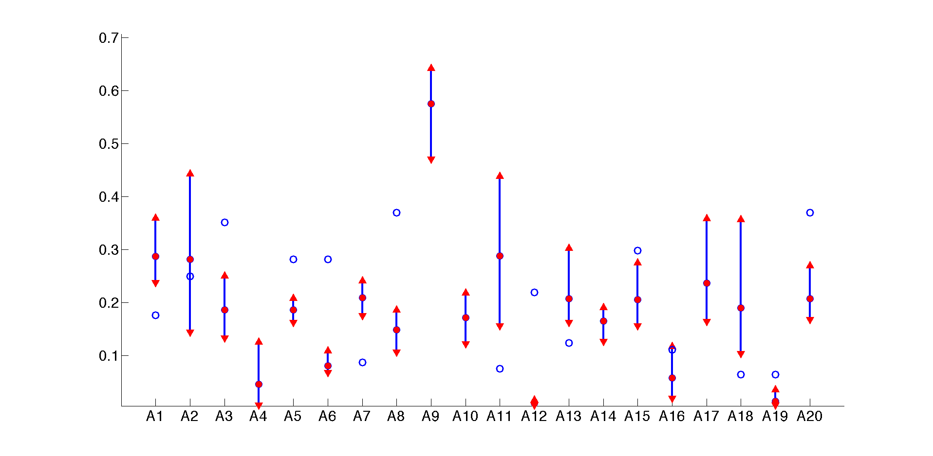
; see Figure 7 for the calculated overage to underage ratios of 20 airlines with 95% probability intervals.

The overage to underage ratio $\varphi_{a}$ is related to airline’s on-time probability by Equation 8: the higher the on-time rate the lower the ratio $\varphi_{a}$. We compare our results to C2K Monthly Statement issued by IATA. In particular, we choose monthly report issued in November 2012, the same period of our data, and convert the reported airlines’ on-time rates into their overage/underage ratios (represented by the circles in Figure 7). The circles deviate from our estimations, the solid dots, following no obvious rules. We believe this is because IATA calculated the on-time rate by simply averaging on-time times of an airline, which fails to exclude the impacts from factors other than the airline, e.g., cargo weight, route, and thus results in unfair comparison. The baseline distribution we calculated can also be used to calculate many other metrics, such as variance, probability of extreme disruptions etc, rather than the simple on-time rate reported by IATA’s monthly report.

6 Conclusions and Future Directions

Using data from international air cargo logistics, we investigate ways to assess and forecast transport risks, defined as the deviation between actual arrival time and planned arrival time. To accommodate the special multimodal feature of the data, we introduce a Bayesian nonparametric mixture model, the Probit stick-breaking process (PSBP) mixture model, for flexible estimation of conditional density function of transport risk. Specifically, we build a linear structure, including demand variables and decision variables, into kernel weights so that the probability weights change with predictors. The model structure is easily extended to account for other factors, such as long-term effects, by allowing coefficients to change dynamically over time, if data allows. Advantages of the PSBP include its generality, flexibility, relatively simple sampling algorithm and theoretical support.

Our results show that our method achieves much more accurate forecasts than alternative models: naive linear model, generalized additive model and flexible mixture model. Moreover, the linear model can lead to misleading inferences. We also demonstrate how an accurate estimation of transport risk Cpdf can help shippers to choose from multiple available services, and help a forwarder to set targeting price, etc. In addition, we show how to use the model to estimate baseline performance of a predictor, such as an airline. We compare our findings with performance reports issued by IATA and point out the shortcomings of IATA’s simple way of ranking airlines. We note that the usage of our method can be much broader than the examples shown here. Indeed, any decisions involving a distribution function require an estimated Cpdf.

Our study serves as a stepping stone to deeper studies in the air cargo transport industry, or more generally, the transportation industry, which generates tons of data everyday yet lacks proper techniques for data analysis. According to a 2011 McKinsey report (Manyika et al. 2011), in the transportation and warehousing sector, the main focus of our paper, IT intensity is among the top 20% and data availability is among the top 40% of all sectors, but the data-driven mind-set is merely at the bottom 20%. The authors’ communication with leaders in this industry, from whom we get the data supporting this research project, confirms this situation, “… we have plenty of data, or we could say we have all the data possible, but we don’t know how to use the data…”.

One of the interesting findings of our paper is that airlines have critical impact on the shape of the transport risk distribution rather than the mean focused on by linear models. For future research, we hope to be able to obtain information regarding why and how airlines are performing so differently on the same routes. By knowing the root drivers of airline service performance, the service quality can be improved for each airline rather than simply choose the best performer.

We are grateful for the generous support of industry sponsors Dr. Prof. Rod Franklin and Mr. Michael Webber. We also thank the area editor Anton Kleywegt, an anonymous associate editor and two referees for their valuable suggestions to make this paper better.

7 Data

7.1 Data Cleaning

After matching MUP with its baseline RMP, we obtain 155,780 shipments (matching rate is higher than 95%). After dropping (1) shipments with extremely delayed milestones (usually caused by data input errors); (2) shipments missing critical information (e.g., carrier); (3) shipments missing weight or package information, 139,512 shipments are retained. The 139,512 shipments are operated by 20 airlines on 11,282 routes (we treat A to B and B to A as two distinct routes), and form 17,604 airline-route pairs. Since our analysis involves the airline-route interaction term, in order to avoid the high noise caused by sparse observations, we drop route-airline pairs containing less than 10 observations and routes containing less than 20 observations in the observing period. After applying this filter, we have 86150 observations left operated by 20 airlines on 1,333 routes. The filter is effective in selecting large and profitable routes.

7.1.1 Exception Records

Exception codes are meant to facilitate (1) finding root causes of delays and (2) identifying parties accountable for failures. Unfortunately, as confirmed by the company as well as our data, exception codes are not helpful in these regards. Less than 8% of delays are assigned exception codes, with only 10% of delays of more than 1 day coded. In addition, codes are ambiguous, with the most frequently appearing code being “COCNR”, denoting the carrier hasn’t received the cargo. Hence, we do not use exception data in our analysis.

7.2 Data Illustration

In Figure

Figure 7.1: Cargo 2000 members

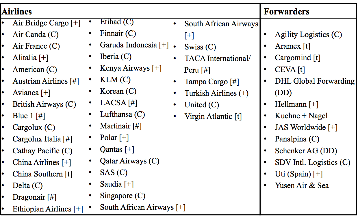
7.1 are the current members under C2K standards. In Table A.1

Table 7.1: An example of a route map

Milestone	Time	Airport	Flight	Weight	Piece
RCS	06.12.2013 16:15:00	NTE	#	630	2
DEP	06.12.2013 19:00:00	NTE	AA 8854	630	2
ARR	07.12.2013 08:52:00	CDG	AA 8854	630	2
DEP	10.12.2013 09:21:00	CDG	AA 0063	630	2
RCF	10.12.2013 21:26:00	MIA	AA 0063	630	2
DEP	11.12.2013 14:58:00	MIA	AA 0913	630	2
RCF	11.12.2013 21:46:00	BOG	AA 0913	630	2
DLV	11.12.2013 22:40:00	BOG	#	630	2

is a typical route map for a shipment from Nantes (France) to Bogotá (Columbia). In Figure

Figure 7.2: Important milestones in a shipment with their short names

7.2 are the milestone chain and explanation of each milestone. In Table 7.2

Table 7.2: A typical record of exception

Status	Exception	Time	Flight	Airport
DEP	COCSYMD	08.01.2013 05:05:00	BA 0125	LHR

is an typical record of an exception.

7.3 Summary Statistics

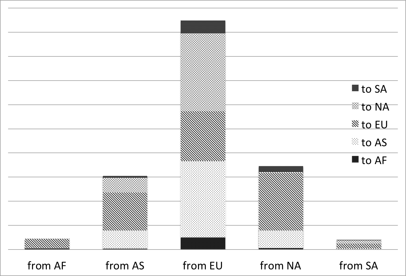
Figure 7.6 shows the number of shipments for each airline, and the percentage of shipments by the number of legs. In Figure 7.6 is the percentage of shipments between the five continents (AF: Africa; AS: Asia; EU: Europe; NA: North America; SA: South America). Figure 7.6 shows the number of airlines available for each shipment. Figure 7.6 depicts the choices between legs of each shipment. Table 7.3 provides summary statistics with predictors defined in Table 1.

Table 7.3: Summary statistics

Dependent Variable
			mean	std
transport risk (hour)			-2.6	20.6
Predictors
	Category Predictor
		airline	route	airline-route	month	airline-leg2	airline-leg3
	dimension	20	1336	588	7	20	16
	Continuous Predictor
		$dev_{start}$ (day)	$dur$ (day)	log$\left(wgt\right)$ (kg)	log$\left(pcs\right)$ (cbm)
	mean	-0.327	1.75	4.91	1.29
	std	0.648	1.30	2.4	1.43

Figure 7.3: Number of shipments by each airline with different number of legs (1, 2 or 3)

Figure 7.4: Number of shipments between continents

Figure 7.5: The percentage of routes with different number of airline options. The airline options vary from only 1 airline to as many as 6 airlines serving the same route.

Figure 7.6: The percentage of routes with different number of leg options (mainly 1 or 2 legs). The histogram is further classified into two categories: whether the route is served by a single airline or multiple airlines.

8 Supplementary Material of Computation and Model Checking

8.1 Gibbs Sampling

8.1.1 Gibbs Sampling for Kernel Parameters

We use “$\cdots$” to indicate all the other parameters and data. The full conditional distribution of the component-specific parameters, $\mu_{l}$ and $\phi_{l}$, is given by

$$p\left(\mu_{l},\phi_{l}\mid\cdots\right)\propto\mathsf{N}\mathsf{G}\left(\mu_{l},\phi_{l}\mid\zeta_{\mu},\xi_{\mu},a_{\phi},b_{\phi}\right)\prod_{({\bf x},j)\;s.t.\;s_{j}\left({\bf x}\right)=l}\mathsf{N}\left(y_{j}\mid\mu_{l},\phi_{l}\right)$$

where $\propto$ represents “proportional to”, $\mathsf{N}\mathsf{G}$ is the Normal-Gamma conjugate prior of $\mu_{l}$ and $\phi_{l}$. Simplified by the conjugacy structure, the Gibbs sampling of kernel mean $\mu_{l}$ is carried out by

$$\mu_{l}\mid\cdots\sim\mathsf{N}\left(\left[\zeta_{\mu}+n_{l}\phi_{l}\right]^{-1}\left[\zeta_{\mu}\xi_{\mu}+h_{l}\phi_{l}\right],\xi_{\mu}+n_{l}\phi_{l}\right)$$

where $n_{l}=\sum_{{\bf x}\in{\cal X}}\sum_{j=1}^{n({\bf x})}\mathbf{1}_{(s_{j}({\bf x})=l)}$ and $h_{l}=\sum_{{\bf x}\in{\cal X}}\sum_{j=1}^{n({\bf x})}y_{j}({\bf x})\mathbf{1}_{(s_{j}({\bf x})=l)}$. Similarly, the Gibbs sampling of kernel precisions $\phi_{l}$ is

$$\phi_{l}\mid\cdots\sim\mathsf{G}\left(a_{\phi}+\frac{n_{l}}{2};b_{\phi}+\frac{1}{2}\sum_{{\bf x}\in{\cal X}}\sum_{j=1}^{n({\bf x})}\left(y_{j}({\bf x})-\mu_{l}\right){}^{2}\mathbf{1}_{(s_{j}({\bf x})=l)}\right)$$

8.1.2 Gibbs Sampling for Weight Parameters: Latent Indicators

Conditional on kernel parameters and the realized values of the weights $\left\{\omega_{l}\left({\bf x}\right),\forall{\bf x}\in{\cal X}\right\}_{l=1}^{L}$, the distribution of the indicators is multinomial with probability given by

$$\mbox{Pr}(s_{j}({\bf x})=l|\cdots)\propto\omega_{l}({\bf x})\mathsf{N}\left(y_{j}({\bf x})|\mu_{l},\phi_{l}\right),$$

So we can sample $s_{j}({\bf x})$ ($j=1,\cdots,n({\bf x}))$ from a multinomial conditional distribution:

$$Pr(s_{j}({\bf x})=l|\cdots)=\frac{\omega_{l}({\bf x})\mathsf{N}(y_{j}({\bf x})|\mu_{l},\phi_{l})}{\sum_{p=1}^{L}\omega_{p}({\bf x})\mathsf{N}(y_{j}({\bf x})|\mu_{l},\phi_{l})}$$

8.1.3 Gibbs Sampling for Weight Parameters: Latent Auxiliary Variable

In order to sample the latent processes $\left\{\gamma_{l}\left({\bf x}\right),\forall{\bf x}\in{\cal X}\right\}_{l=1}^{L}$ and the corresponding weights $\left\{\omega_{l}\left({\bf x}\right),\forall{\bf x}\in{\cal X}\right\}_{l=1}^{L}$, we augment the data with a collection of conditionally independent latent variables $z_{jl}({\bf x})\sim\mathsf{N}(\gamma_{l}({\bf x}),1)$ ($j=1,\cdots,n({\bf x}))$. We aim to make the probability of observing {$z_{j1}\left({\bf x}\right)$, $\cdots$, $z_{jl}\left({\bf x}\right)$} equal to $\omega_{l}\left({\bf x}\right)$ in Equation (3), thus the event of observing {$z_{j1}\left({\bf x}\right)$, $\cdots$, $z_{jl}\left({\bf x}\right)$} can represent the event of observing $s_{j}({\bf x})=l$ as denoted at the beginning of ${\cal x}3.4$. Specifically if $z_{jp}({\bf x})<0$ for all $p<l$ and $z_{jl}({\bf x})>0$, we define $s_{j}({\bf x})=l$. For a finite $L$ case, we define $s_{i}({\bf x})=L$ if $z_{ip}({\bf x})<0$ for all $p\leq L-1$. Then we have

$$\mbox{Pr}(s_{j}({\bf x})=l) = \mbox{Pr}\left(z_{jl}({\bf x})>0,z_{jp}({\bf x})<0\mbox{ for }p<l\right)$$

$$= \Phi\left(\gamma_{l}({\bf x})\right)\prod_{p<l}\left\{1-\Phi\left(\gamma_{p}({\bf x})\right)\right\}$$

independently for $j=1,\cdots,n({\bf x})$. In this way, $\mbox{Pr}(s_{j}({\bf x})=l)$ equals to $\omega_{l}\left({\bf x}\right)$ as defined in Equation (3). This data augmentation scheme simplifies computation as it allows us to implement the following Gibbs sampling scheme

$$z_{jl}({\bf x})\mid\cdots\sim\mathsf{N}\left(\gamma_{l}({\bf x}),1\right)\mathbf{1}_{\boldsymbol{\Omega}_{l}},\;\forall l\leq\mbox{min}\{s_{j}({\bf x}),L-1\},$$

with

$$\boldsymbol{\Omega}_{l}=\begin{cases}\{z_{jl}({\bf x})<0\},&\mbox{if }l<s_{j}({\bf x}),\\ \{z_{jl}({\bf x})\geq 0\},&\mbox{if }l=s_{j}({\bf x})<L\end{cases}$$

where $\mathsf{N}\left(\cdot\right){\bf 1}_{\Omega}$ denotes a normal distribution truncated to the set $\Omega$.

8.1.4 Gibbs Sampling for Weight Parameters: Latent Processes

The latent process $\left\{\gamma_{l}\left({\bf x}\right),\forall{\bf x}\in{\cal X}\right\}$ is built on parameters $\Theta=${$\left\{\theta_{l}^{1}\right\}$, $\left\{\theta_{a}^{2}\right\}$, $\left\{\theta_{r}^{3}\right\}$, $\left\{\theta_{\left(a,r\right)}^{4}\right\}$, $\left\{\theta_{m}^{5}\right\}$, $\left\{\theta_{leg}^{6}\right\}$, $\left\{\theta_{\left(a,leg\right)}^{7}\right\}$, $\boldsymbol{\theta}^{8}$, $\boldsymbol{\theta}^{9}$, $\boldsymbol{\theta}^{10}$, $\boldsymbol{\theta}^{11}$, $\boldsymbol{\theta}^{12}$} and hyper-parameters $\Upsilon$ = {$\epsilon^{i}$, $\forall i$ = =1, 2, $\cdots$, 7}. The distribution of $\Theta$ and $\Upsilon$, conditional on the augmented data, is given by

$$p(\Theta,\Upsilon\mid\cdots)\propto\left[\prod_{{\bf x},j}p\left({\bf z}_{j}({\bf x})\mid\boldsymbol{\gamma}_{j}({\bf x})\right)\right]p(\Theta)p\left(\Upsilon\right)$$

where $p\left(\Theta\right)$ is the prior distribution of $\Theta$ and $p\left(\Upsilon\right)$ is the prior distribution of $\Upsilon$, and $j=1,\cdots,n({\bf x})$. The posterior sampling can be easily implemented by taking advantage of the normal priors we choose. Due to similarities of the Gibbs sampling schemes for $\Theta$ and $\Upsilon$, here we only give updating schemes for two examples: one for coefficients $\left\{\theta_{l}^{1}\right\}_{l=1}^{L}\in\Theta$ and the other one for hyper-parameter $\epsilon^{1}\in\Upsilon$.

1. For $\theta_{l}^{1}$ ($l=1,2,\cdots,L$), the posterior Gibbs sampling follows normal distribution given by

   $$\theta_{l}^{1}\mid\cdots \propto \mathsf{N}\left(\mu_{\theta_{l}^{1}},\phi_{\theta_{l}^{1}}\right)$$

   where $\mu_{\theta_{l}^{1}}=\left\{\Phi^{-1}\left(\frac{1}{L-l+1}\right)+\sum_{{\bf x}\in{\cal X}}\sum_{j}\left[z_{jl}\left({\bf x}\right)-\Delta_{jl}\left({\bf x}\right)\right]{\bf 1}\left(s_{j}\left({\bf x}\right)\geq l\right)\right\}/\left(n_{l}+1\right)$, $\phi_{\theta_{l}^{1}}=\left(n_{l}+\epsilon^{1}\right)/\left(n_{l}+1\right)$, $n_{l}=\sum_{{\bf x}\in{\cal X}}\sum_{j}{\bf 1}\left(s_{j}\left({\bf x}\right)\geq l\right)$ and $\Delta_{jl}\left({\bf x}\right)=\left(\gamma_{j}\left({\bf x}\right)-\theta_{l}^{1}\right){\bf 1}\left(s_{j}\left({\bf x}\right)\geq l\right)$.

2. For $\epsilon^{1}$ the posterior Gibbs sampling follows Gamma distribution given by

   $$\epsilon^{1}\mid\cdots \propto \mathsf{G}\left(c_{1}+\frac{L}{2},d_{1}+\frac{\sum_{l=1}^{L}\theta_{l}^{1}\cdot\theta_{l}^{1}}{2}\right)$$

In the case $L=\infty$, we can easily extend this algorithm to generate a slice sampler, as discussed in Papaspiliopoulos (2008). Alternatively, the results in Rodriguez and Dunson (2011) suggest that a finite PSBP with a large number of components (30 – 40, depending on the value of $\mu$) can be used instead (Ishwaran and Zarepour 2002). So we use $L=50$ as the number of components in this paper; this provides a conservative upper bound as many of these components may not be utilized.

In general, in the conditional method, the Markov chain Monte Carlo algorithm has to explore multimodal posterior distributions. Therefore, we need to add label-switching moves, which assist the algorithm in jumping across modes. This is particularly important for large data sets, where the modes are separated by areas of negligible probability. We use the framework developed in Papaspiliopoulos and Roberts (2008) to design our label switching moves. These label switching moves greatly improved the convergence of the chain.

8.1.5 Label Switching Moves

The label switching moves with infinite mixture models are listed as follows:

1. From $1,2,\dots,L$ choose two elements $l_{1}$ and $l_{2}$ uniformly at random and change their labels with probability

   $$\min\left(1,\Pi_{{\bf x}\in{\cal X}}\left(\frac{\omega_{l_{1}}\left({\bf x}\right)}{\omega_{l_{2}}\left({\bf x}\right)}\right)^{n_{l_{2}}\left({\bf x}\right)-n_{l_{1}}\left({\bf x}\right)}\right)$$

   where $n_{l}\left({\bf x}\right)=\sum_{j}s_{j}\left({\bf x}\right)=l$ ($j=1,\cdots,n\left({\bf x}\right)$)

2. Sample a label $l$ uniformly from $1,2,\dots,L-1$ and propose to swap the labels $l$, $l+1$ and corresponding stick-breaking weights $\gamma_{l}$, $\gamma_{l+1}$ with probability

   $$\min\left(1,F\times\Pi_{{\bf x}\in{\cal X}}\frac{\left(1-\Phi\left(\gamma_{l+1}\left({\bf x}\right)\right)\right)^{n_{l}\left({\bf x}\right)}}{\left(1-\Phi\left(\gamma_{l}\left({\bf x}\right)\right)\right)^{n_{l+1}\left({\bf x}\right)}}\right)$$

   where

   $$F=\frac{\mathsf{N}\left(\theta_{l}^{1}\mid\Phi^{-1}\left(\frac{1}{L-l}\right),1\right)\cdot\mathsf{N}\left(\theta_{l+1}^{1}\mid\Phi^{-1}\left(\frac{1}{L-l+1}\right),1\right)}{\mathsf{N}\left(\theta_{l}^{1}\mid\Phi^{-1}\left(\frac{1}{L-l+1}\right),1\right)\cdot\mathsf{N}\left(\theta_{l+1}^{1}\mid\Phi^{-1}\left(\frac{1}{L-l}\right),1\right)}$$

   is the change of prior probability since the prior of $\theta^{1}$ is not symmetric.

Label switching moves for finite mixture models are listed as follows:

1. Sample a label $l$ uniformly from $1,2,\dots,L-1$ and propose to swap the labels $l$, $l+1$ and corresponding stick-breaking weights $\gamma_{l}$, $\gamma_{l+1}$ with probability

   $$\min\left(1,F\times\Pi_{{\bf x}\in{\cal X}}\frac{\left(1-\Phi\left(\gamma_{l+1}\left({\bf x}\right)\right)\right)^{n_{l}\left({\bf x}\right)}}{\left(1-\Phi\left(\gamma_{l}\left({\bf x}\right)\right)\right)^{n_{l+1}\left({\bf x}\right)}}\right),\;\mbox{if }l\leq L-2$$

   where

   $$F=\frac{f\left(\alpha_{l}\mid\Phi^{-1}\left(\frac{1}{L-l}\right),1\right)f\left(\alpha_{l+1}\mid\Phi^{-1}\left(\frac{1}{L-l+1}\right),1\right)}{f\left(\alpha_{l}\mid\Phi^{-1}\left(\frac{1}{L-l+1}\right),1\right)f\left(\alpha_{l+1}\mid\Phi^{-1}\left(\frac{1}{L-l}\right),1\right)}$$

   is the change of prior probability and $f(\cdot\mid\mu,\phi)$ is the probability density function of $\mathsf{N}\left(\cdot\mid\mu,\phi\right)$. If $l=L-1$, the Metropolis-Hasting probability is:

   $$\min\left(1,\Pi_{{\bf x}\in{\cal X}}\left[\frac{\Phi\left(\gamma_{l}\left({\bf x}\right)\right)}{1-\Phi\left(\gamma_{l}\left({\bf x}\right)\right)}\right]^{n_{l+1}\left({\bf x}\right)-n_{l}\left({\bf x}\right)}\right),\;\mbox{if }l=L-1$$

8.2 Prior Elicitation

First, we consider eliciting hyper-parameters $\left\{\zeta_{\mu_{l}}\right\}_{l=1}^{L}$ and $\left\{\xi_{\mu_{l}}\right\}_{l=1}^{L}$, corresponding to the location of the Normal components, and $a_{\phi}$ and $b_{\phi}$, corresponding to their precisions. These hyper-parameters need to be chosen to ensure that the mixture spans the expected range of observed values with high probability. In our case, we have all prior means $\left\{\zeta_{\mu_{l}}\right\}_{l=1}^{L}$ equal to the global mean (or global median) of all observations, -2.64, and set all $\left\{1/\xi_{\mu_{l}}\right\}_{l=1}^{L}$ equal to half the range of the observed data (a rough estimate of dispersion), 189.6. Sensitivity was assessed by halving and doubling the values of $\xi_{\mu_{l}}$. Under a similar argument, $a_{\phi}$ and $b_{\phi}$ should be chosen so that $E\left(1/\phi_{l}\right)=b_{\phi}/\left(a_{\phi}-1\right)$ is also around half the range of the observations, so we choose $a_{\phi}=1.25,\;b_{\phi}=47.5$. In every scenario we have employed proper priors, as weakly informative proper priors lead to improved performance and improper priors can lead to paradoxical behavior in mixture models, similar to the well known Bartlett-Lindley paradox in Bayesian model selection.

Next, we consider the prior structure on the weights $\omega_{l}\left({\bf x}\right)$. As discussed above, the use of a continuation ratio Probit model along with normal priors for the transformed weights is convenient, as it greatly simplifies implementation of the model. In particular, the transformed mixture weights $\{\gamma_{l}\left({\bf x}\right)\}$ can be sampled by the algorithm shown in ${\cal x}$3.2.3 above from conditionally normal distributions. Hyper-parameter choice is also simplified. A common assumption of basic mixture models for $i.i.d.$ data is that all components have the same probability a priori. In the current context in which mixture weights are predictor dependent, a similar constraint can be imposed on the baseline conditional distribution by setting $E(\theta_{l}^{1})=\Phi^{-1}\left(1/\left(L-l+1\right)\right)$. Since we build a hierarchy above heterogeneity parameters to allow information borrowing, the variance of $\theta^{i}$ ($i=1,2,\cdots,7$), is controlled by the distribution of hyper parameters $\epsilon^{i}$. In order to make sure the continuation ratio $\Phi(\gamma_{l}\left({\bf x}\right))$ is between 0.001 and 0.998 with 0.99 probability, we would expect $\text{Var}\left(\theta^{i}\right)\approx 1$. Smaller values for $V(\theta^{i})$ lead to strong restrictions on the set of weights, discouraging small ones (especially for the first few components in the mixture). On the other hand, larger variances can adversely affect model selection. For the hyper parameter $\epsilon^{i}$ of $\theta^{i}$, in order to make sure $\text{Var}\left(\theta^{i}\right)\approx 1$, we let $c_{i}=6,\;d_{i}=5$ so that $\text{E}\left(1/\epsilon^{i}\right)=1$. This yields a prior sample size of 6, which gives some stability while very small restrictions.

8.3 Implementation

The data were analyzed using the models described in ${\cal x}$3.1. Fifty mixture components were judged sufficient to flexibly characterize changes in the density across predictors, while limiting the risk of over-fitting. Inferences were robust in our sensitivity analysis for $L$ ranging between 40 and 60, but the quality of the fit, as assessed through the plots described in ${\cal x}$3 and ${\cal x}$5, was compromised for $L<40$.

The Gibbs samplers were run for 100,000 iterations following a 70,000 iteration burn-in period. Code was implemented in Matlab, and the longest running time was 118h on a 2.96-GHz Intel Xeon E5-2690 computer with 32 cores. This run time could be dramatically reduced by improving code efficiency and relying on recent developments in scalable Bayesian computation, but we preferred to use standard Gibbs sampling instead of new and less well established computational methods. Examination of diagnostic plots showed adequate mixing and no evidence of lack of convergence.

8.4 Cross Validation for Variable Selection

To balance computation time and accuracy, we use 3-fold cross validation based on predictive log likelihood. Specifically, we partition the original data into three equal sized subsamples, with two of the subsamples used as training data for parameter estimation. Then, the estimated parameters are used to calculate the log likelihood, as shown in Equation (5), of the left out subsample, also known as the validation data. This process is repeated for 3 times so that every subsample is used as validation data once. The reason why we choose to calculate the log likelihood of the validation data that log likelihood is a strictly proper scoring rule for density forecasts as in our study, as explained in Gneiting and Raftery (2007). We compare the cross validation value of many models and list 10 models in Table 8.1.

Table 8.1: Cross validation for model comparison

	Model	-$LL$		Model	-$LL$
1	$\Xi$	324235	6	$\Xi-\theta_{\left(a,leg\right)}^{7}-\theta_{\left(a,r\right)}^{4}$	326687
2	$\Xi-\theta_{\left(a,leg\right)}^{7}$	318101	7	$\Xi-\theta_{\left(a,leg\right)}^{7}-\theta_{leg}^{6}-\theta^{11}$	319515
3	$\Xi-\theta_{\left(a,leg\right)}^{7}-\theta_{leg}^{6}$	320239	8	$\Xi-\theta_{\left(a,leg\right)}^{7}-\theta_{m}^{5}-\theta^{11}$	318684
4	$\Xi-\theta_{\left(a,leg\right)}^{7}-\boldsymbol{\theta}^{11}$	317894	9	$\Xi-\theta_{\left(a,leg\right)}^{7}-\theta_{leg}^{6}-\theta_{m}^{5}$	327174
5	$\Xi-\theta_{\left(a,leg\right)}^{7}-\theta_{m}^{5}$	318894	10	$\Xi-\theta_{\left(a,leg\right)}^{7}-\theta_{\left(a,r\right)}^{4}-\theta_{a}^{2}$	328721

For each model, the log-likelihood of its three subsamples is calculated by averaging over 10,000 posterior samples with the first 10,000 posterior samples dropped as burn-in. In Table 8.1 we use $\Xi$ to indicate the full model, as shown in Equation (4), and use “$-$” to indicate dropping certain predictors. We use $LL$ to indicate sum of the three subsample log-likelihood for each model. Since we are comparing $-LL$ in Table 8.1, smaller values suggest stronger predictive capability. So we choose model (4) in the Table 8.1, which is equivalent to Equation (9).

$$\gamma_{l}({\bf x}) = \theta_{l}^{1}+\theta_{a}^{2}+\theta_{r}^{3}+\theta_{\left(a,r\right)}^{4}+\theta_{m}^{5}+\theta_{leg}^{6}+f_{1}\left(dev_{start}\mid\boldsymbol{\theta}^{8}\right)+f_{2}\left(dur\mid\boldsymbol{\theta}^{9}\right)+f_{3}\left(\mbox{log}\left(wgt\right)\mid\boldsymbol{\theta}^{10}\right)$$ (9)

Since there are 11 kinds of predictors in the full model (i.e., Equation (4)), which are $2^{11}=2048$ different possible variable combinations, it is impossible for us to compare every model in a relatively short research time frame. We choose to use a backward fitting process. Specifically, we start with the full model, then every time we drop one predictor and observe how the $-LL$ change. If the $-LL$ decreases, then we keep this predictor removed, otherwise, we add this predictor back. For example, from model 1 to 2 in Table 8.1, while the interaction term of airline and legs is dropped the $-LL$ drops, so we remove the interaction of airline and leg. From model 2 to 3, we further drop predictor “legs”, however $-LL$ increases, as a result, we add predictor “legs” back. We tested many more models than those listed in Table 8.1 with the best model shown in Equation (9). The 10 models listed in Table 8.1 are shown for illustration.

As we have mentioned in $\mathsection$3.2, $f_{1}$, $f_{2}$ , $f_{3}$ in Equation (9) ($f_{4}$ in Equation (4) is similar) are spline functions expressed as a linear combination of B-splines, or basis spline, of degree 4. The usefulness of B-spline lies in the fact that any spline function of order $n$ on a given set of knots can be expressed as a unique linear combination of B-splines, hence the name basis spline. The knots of $f_{1}$, $f_{2}$, $f_{3}$ and $f_{4}$ have been listed in $\mathsection$3.2, the knots are chosen based on both the meaning in reality (e.g., for better interpretation) and to make sure the data amount in each range of support is roughly comparable. The final expression of the basis spline of a higher order (3 or higher) can be very complicated, so here I only list the recursion formula:

$$B_{i,1}(x) = \begin{cases}1&\mbox{if }t_{i}\leq x<t_{i+1}\\ 0&\mbox{otherwise}\end{cases}$$

$$B_{i,k}(x) = \frac{x-t_{i}}{t_{i+k-1}-t_{i}}B_{i,k-1}(x)+\frac{t_{i+k}-x}{t_{i+k}-t_{i+1}}B_{i+1,k-1}(x)$$

where vector ${\bf t}$ is the knots and $k$ is the order of B-spline. We have tried different orders of B-splines (i.e., $3\sim 6$) with slightly changed knots, however, the predictive power is almost the same. So we decide to use a B-spline of order 4.

8.5 Model Checking and Comparison

In this section, $\mathsection$B.5.1 and $\mathsection$B.5.2 are on model checking while $\mathsection$B.5.3 is about model comparison.

8.5.1 Posterior Predictive Checks

We first use posterior predictive checks (PPC), devised in Rubin (1984) and expanded in Gelman et al. (1996). PPC provide a popular approach for goodness-of-fit assessments of Bayesian models. In implementing PPC, one first generates multiple data sets of the same structure as the observed dataset from the posterior predictive distribution. This is done by generating parameters from the posterior distribution, plugging these parameters into the likeihood, and then sampling new data from this likelihood. If the model does not fit the data well, data generated from the posterior predictive distribution will deviate systematically from the observed data. As an illustration, we implemented a PPC check of a naive linear model (referred to as LM), a method widely used in previous research on flight delays. The specific form of LM is as follows:

$$y \sim N(\mu,\sigma^{2})$$

$$\mu = \theta^{1}+\theta_{a}^{2}+\theta_{r}^{3}+\theta_{\left(a,r\right)}^{4}+\theta_{m}^{5}+\theta_{leg}^{6}+\theta^{8}\cdot dev_{start}+\theta^{9}\cdot dur+\theta^{10}\cdot\mbox{log}\left(wgt\right)$$ (10)

where $y$ represents the dependent variable transport risk. All the other predictors $\boldsymbol{\theta}$ are the same as explained in $\mathsection 3.2$ except the original vector $\theta^{1}$ now doesn’t have the subscript $l$ for each cluster and is just a scalar intercept.

Figure 8.1: Posterior predictive model checking. In “LM Replicate” and “PSBP Replicate”, the histogram is the predicted response, transport risk. In the other four plots, the title is the target value for posterior predictive checking; the histogram is PSBP predictive values; the solid line is the value calculated from the real data; the dash-dotted line is the predictive value by LM.

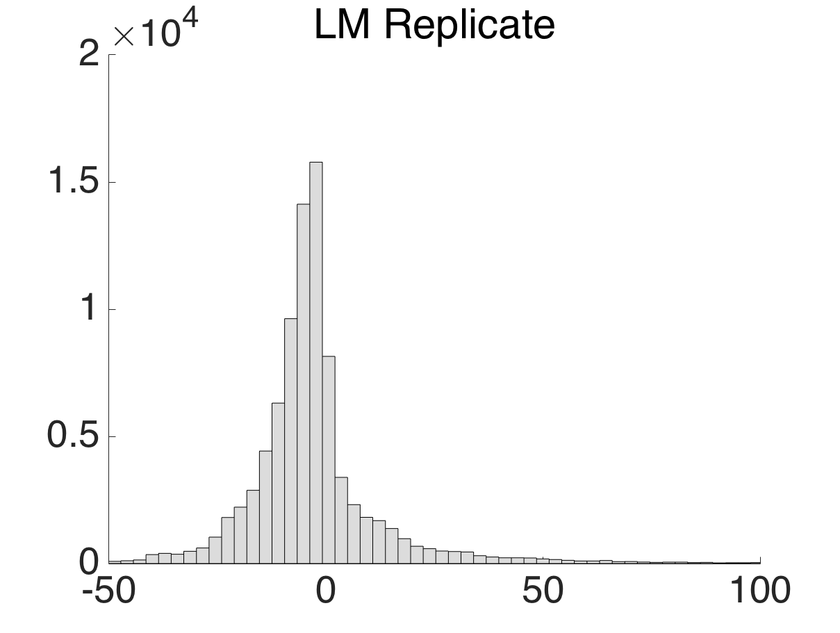
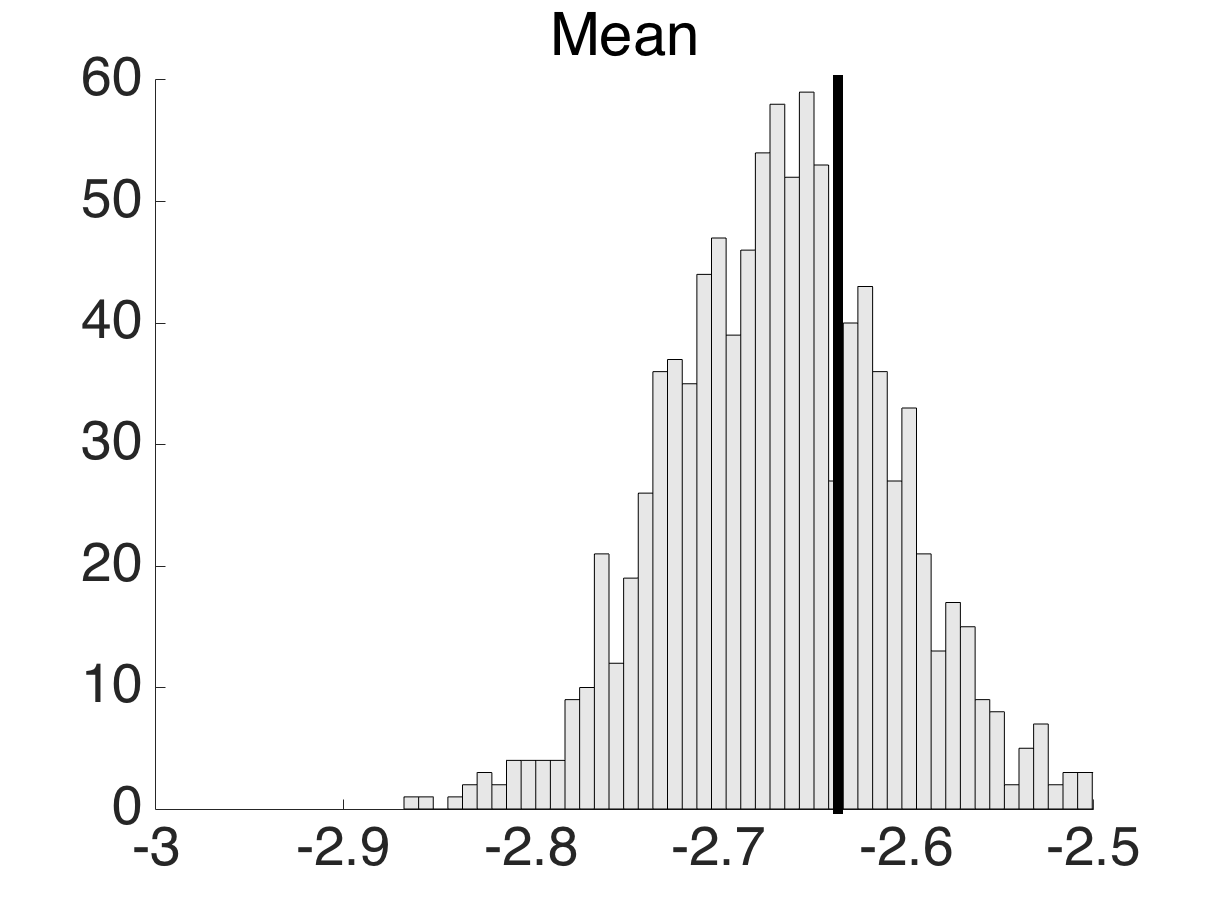
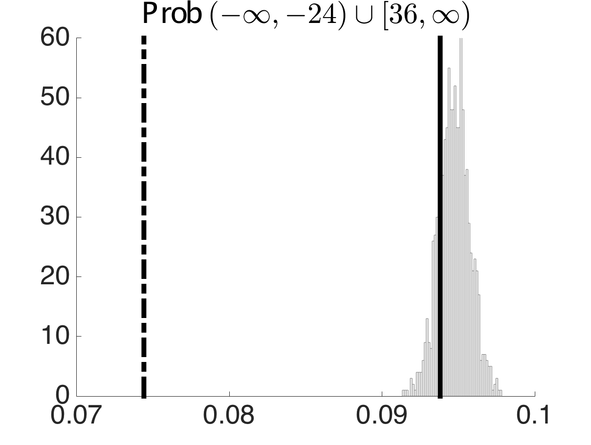
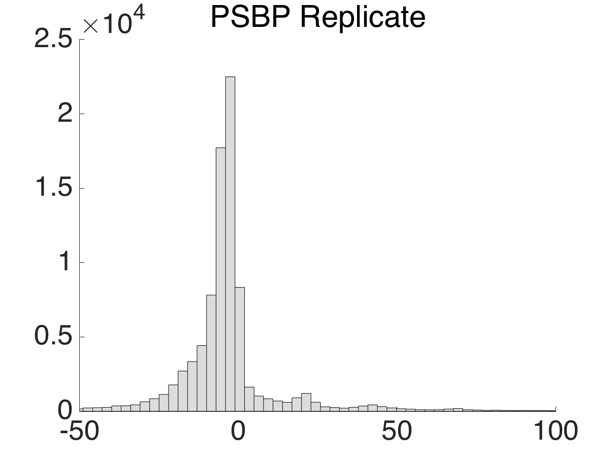
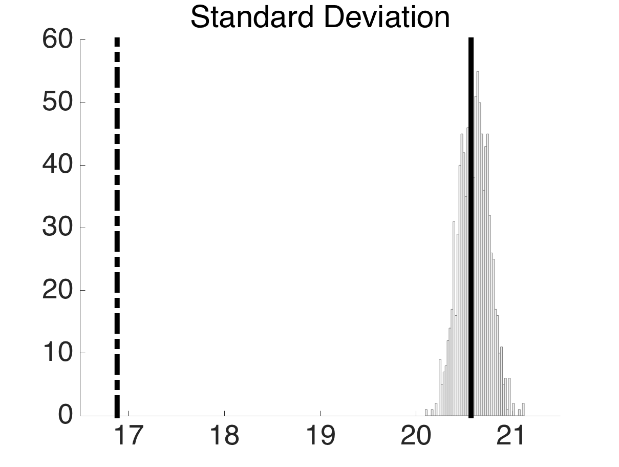
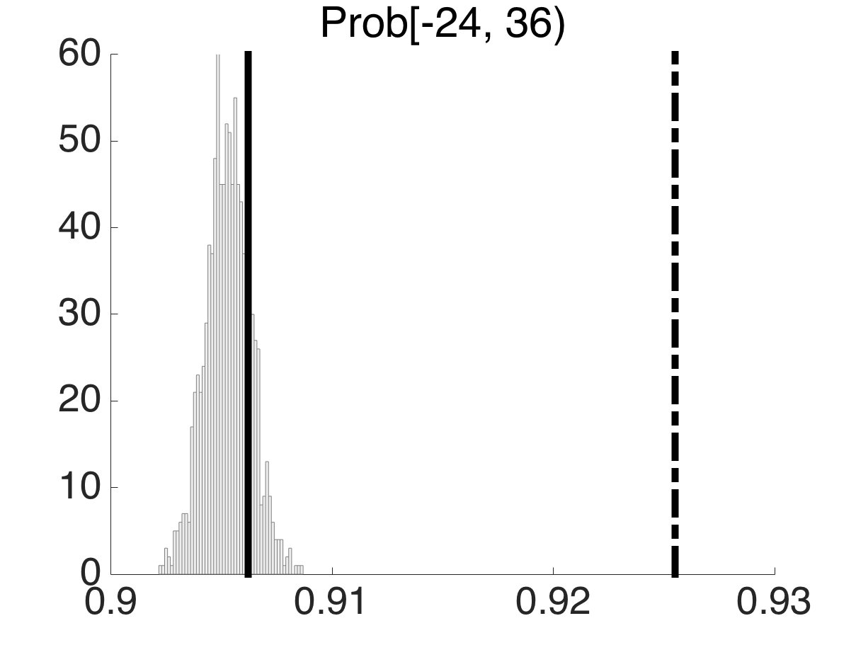
To follow the steps of PPC, we replicate two data sets: one predicted by LM and one predicted by our model. We use these two replicated data to calculate summary statistics including mean, standard deviation, $\mathsf{Prob}\left(\hat{y}<-24\mbox{ or }\hat{y}\geq 36\right)$ (i.e., the probability of transport disruption) and $\mathsf{Prob}\left(-24\leq\hat{y}<36\right)$ (i.e., the probability of recurrent transport risks), then compare the values to the statistics calculated using the true data. If the model fits well, we expect the empirical values of these statistics to not deviate significantly from the simulated distribution under the assumed model. From Figure 8.1 we found that LM predicts the mean accurately (the dashed line and solid line overlays), however largely underestimates extreme situations like more than 24 hours earliness or more than 36 hours delays, while overestimating recurrent risk such as deviations between -24 to 36 hours. In addition, standard deviation is substantially underestimated. On the other hand, the posterior predictive statistics by PSBP closely surrounding the empirical values. Moreover, if we just look at the empirical distribution of the two replica data as compared to the observed data empirical distribution (the first column in Figure 8.1), we can see that the replicated data by LM resembles the shape of the real data poorly. Whereas, the replicated data by our model resembles the real data very well. This clearly shows the model inadequacy of linear model in our situation and confirms our PSBP model to fit the data well.

8.5.2 Visual Inspection

We further check the model at a more granular level – airline-route level. In Figure 3, the histogram is drawn from real data, the solid line is the predictive conditional density by PSBP (the posterior 95$\%$ probability intervals are too narrow to be visible in this figure), while the dashed line is predicted by LM. PSBP captures the location and weights of peaks accurately while linear model predicts badly.

8.5.3 Model Comparison

We further formally compare our model with alternative models including LM, generalized additive model (GAM) and flexible mixture model (Flexmix) using predictive residuals. GAM, as shown in Equation (11)

$$y \sim N(\mu,\sigma^{2})$$

$$\mu = \theta^{1}+\theta_{a}^{2}+\theta_{r}^{3}+\theta_{\left(a,r\right)}^{4}+\theta_{m}^{5}+\theta_{leg}^{6}+s(dev_{start}\mid\theta^{8})+s\left(dur\mid\boldsymbol{\theta}^{9}\right)+s\left(\mbox{log}\left(wgt\right)\mid\boldsymbol{\theta}^{10}\right)$$ (11)

generalizes LM by incorporating nonlinear forms of the continuous predictors. Here $s(\cdot\mid\boldsymbol{\theta})$ represents the smooth function (also the nonparametric or nonlinear form) and $\boldsymbol{\theta}$ are the parameters. We estimate the model using the “bam” function in R package “mgcv” (Wood 2011), in which the estimation of GAMs is conducted via a penalized likelihood frequentist approach. The flexible mixture model we consider is shown as follows (we use the same number of clusters as in PSBP mixture model):

$$y \sim \sum_{l}\omega_{l}N(\mu_{l},\sigma_{l})$$

$$\mu_{l} = \theta_{l}^{1}+\theta_{a}^{2}+\theta_{r}^{3}+\theta_{\left(a,r\right)}^{4}+\theta_{m}^{5}+\theta_{leg}^{6}+s(dev_{start}\mid\theta^{8})+s\left(dur\mid\boldsymbol{\theta}^{9}\right)+s\left(\mbox{log}\left(wgt\right)\mid\boldsymbol{\theta}^{10}\right)$$ (12)

This expression is similar to Equation (5). However, the regression part is now in the Gaussian mean rather than the mixture weights. We estimate the model using “flexmix” function in R package “flexmix” (Gruen and Leisch 2008), in which maximum likelihood estimation is conducted via an EM algorithm.

Table 8.2: Residual checks for model comparison

	LM	GAM	Flexmix	PBSP Mixture
I/O* RMSE	18.6/19.1	17.8/18.4	14.9/15.7	14.1/15.0
I/O MAE	9.66/10.00	9.01/9.31	7.73/8.02	7.17/7.56
I/O Log-likelihood	373090/387755	370547/385183	314477/325575	307124/317894
* I/O: in-sample/out-of-sample

Table 8.2 shows the root mean squared error (RMSE), mean absolute error (MAE) and log likelihood of the in-sample and out-of-sample prediction of the four models. Here the out-of-sample prediction is the average RMSE/MAE/log-likelihood value from the three 3-fold cross-validation methods explained in Appendix $\mathsection$B.4.

From the table, the PSBP Mixture model clear beats the alternatives in all metrics in both in-sample and out-of-sample tests. The under-performance of LM and GAM are easy to understand, as likely arising from the lack of ability to allow the delay distribution to shift flexibly with predictors. Flexmix is a more realistic competitor in this respect, but has some clear disadvantages relative to our Bayesian PSBP mixture approach. Both models are richly parameterized and even though the sample size is large overall, there can be sparsity in local regions of the predictor space. Hence, maximum likelihood estimation may have inflated errors relative to a penalization approach. The weakly informative priors we advocate protect against overfitting and reduce mean square error in estimating coefficients. Another advantage of PSBP is the form of the model in which the kernels are fixed and the weights vary with predictors. As explained in $\mathsection$3.1, the locations of peaks of the multi-modal distribution of the dependent variable, transport risk, are almost constant. However, the heights of the peaks change greatly with predictors (e.g., route, airline, demand variables). Our model can more parsimoniously account for such changes.

In terms of the computational time, we have explained those of our model in Appendix $\mathsection$B.3. LM, GAM and Flexmix are implemented in R using packages listed above on a server of 128G memory. The computational time of LM and GAM are fairly short, 3 minutes and 15 minutes respectively. On the other hand, the estimation of Flexmix takes 135h to reach final convergence. As the sample size and number of predictors increase, the rate of convergence and time per iteration can both increase substantially for standard algorithms for fitting mixture models; both frequentist and Bayesian. We note that our code has not been optimized and we have not attempted to use recently developed algorithms for scaling up Bayesian computation to bigger problem sizes. We also note that our PSBP mixture model can be implemented using a frequentist optimization approach; although maximum likelihood estimation via the EM algorithm would be one possibility, the number of predictors and parameters in the model makes it important to include penalties. We do not consider such possibilities further in this article.

9 Supplementary Material of Results

9.1 Model Parameter Estimation

Table 9.1 shows the posterior mean and 95% probability interval of (selected) model parameters.

Table 9.1: Posterior summaries of model parameters

Kernel Parameters
	$\mu_{l}$ $\left(l=1,2,\cdots,50\right)$		min$\left(\mu_{l}\right)=-79.6,\qquad$ max$\left(\mu_{l}\right)=76.01$
	$\nicefrac{{1}}{{\sqrt{\phi_{l}}}}$ $\left(l=1,2,\cdots,50\right)$		min$\left(\nicefrac{{1}}{{\sqrt{\phi_{l}}}}\right)=0.72,\qquad$ max$\left(\nicefrac{{1}}{{\sqrt{\phi_{l}}}}\right)=84.4$
Parameters in Weight $\gamma$
	Category Predictors
	$\theta_{l}^{1}$ $\left(l=1,2,\cdots,49\right)$		min$\left(\theta_{l}^{1}\right)=-10.9,\qquad$max$\left(\theta_{l}^{1}\right)=6.74$
	$\theta_{a}^{2}$ $\left(a=1,2,\cdots,20\right)$
	$\theta_{1}^{2}$ A1	$\theta_{2}^{2}$ A2	$\theta_{3}^{2}$ A3	$\theta_{4}^{2}$ A4	$\theta_{5}^{2}$ A5
	0 (0, 0)	0.03 (-0.40, 0.61)	-5.27 (-5.86, -4.83)	5.15 (4.31, 6.11)	3.09 (2.89, 3.26)
	$\theta_{6}^{2}$ A6	$\theta_{7}^{2}$ A7	$\theta_{8}^{2}$ A8	$\theta_{9}^{2}$ A9	$\theta_{10}^{2}$ A10
	1.16 (0.84, 1.53)	8.53 (8.19, 8.91)	2.54 (2.01, 2.98)	-0.82 (-1.22, -0.40)	2.90 (2.23, 3.64)
	$\theta_{11}^{2}$ A11	$\theta_{12}^{2}$ A12	$\theta_{13}^{2}$ A13	$\theta_{14}^{2}$ A14	$\theta_{15}^{2}$ A15
	-3.35 (-4.02, -2.74)	5.74 (5.44, 5.97)	-2.96 (-3.19, -2.67)	2.74 (2.27, 2.98)	-2.82 (-3.26, -2.36)
	$\theta_{16}^{2}$ A16	$\theta_{17}^{2}$ A17	$\theta_{18}^{2}$ A18	$\theta_{19}^{2}$ A19	$\theta_{20}^{2}$ A20
	4.95 (4.35, 5.50)	-3.16 (-3.50, -2.76)	-5.36 (-6.59, -4.41)	6.23 (5.79, 6.67)	-2.34 (-2.58, -2.12)
	$\theta_{leg}^{5}$ ($leg=2,3$)
	$\theta_{2}^{5}$	$\theta_{3}^{5}$
	-0.29 (-0.38, -0.21)	-0.34 (-0.47, -0.21)
	Hyper-parameters
	$1/\sqrt{\epsilon^{1}}$	$1/\sqrt{\epsilon^{2}}$	$1/\sqrt{\epsilon^{3}}$	$1/\sqrt{\epsilon^{4}}$	$1/\sqrt{\epsilon^{5}}$	$1/\sqrt{\epsilon^{6}}$
	4.86 (3.98, 5.93)	3.39 (2.62, 4.44)	6.26 (5.86, 6.63)	7.02 (6.46, 7.60)	0.64 (0.46, 0.90)	0.74 (0.51, 1.10)

9.2 Application: Baseline Distributions

In Figure 9.1 and Figure 9.2 are the baseline risk distributions of the remaining 17 airlines.

Figure 9.1: Reference performances of sample airlines with predictive density mean (solid) and 95% credible interval (dotted) (cont.)

Figure 9.2: Reference performances of sample airlines with predictive density mean (solid) and 95% credible interval (dotted)

References

- Chung and Dunson (2009) Chung, Y, DB Dunson. 2009. Nonparametric Bayes conditional distribution modeling with variable selection. J. Amer. Statist. Assoc. 104(488) 1646–1660.
- Cohen and Kunreuther (2007) Cohen, MA, H Kunreuther. 2007. Operations risk management: Overview of Paul Kleindorfer’s contributions. Production Oper. Management 16(5) 525–541.
- Deshpande and Arikan (2012) Deshpande, V, M Arikan. 2012. The impact of airline flight schedules on flight delays. Manufacturing Service Oper. Management 14(3) 423–440.
- Escobar and West (1995) Escobar, MD, M West. 1995. Bayesian density estimation and inference using mixtures. J. Amer. Statist. Assoc. 90(430) 577–588.
- Fan et al. (1996) Fan, J, Q Yao, H Tong. 1996. Estimation of conditional densities and sensitivity measures in nonlinear dynamical systems. Biometrika 83(1) 189–206.
- Federgruen and Yang (2009) Federgruen, A, N Yang. 2009. Optimal supply diversification under general supply risks. Oper. Res. 57(6) 1451–1468.
- Gelman et al. (1996) Gelman, A, XL Meng, H Stern. 1996. Posterior predictive assessment of model fitness via realized discrepancies. Statistica Sinica 733–760.
- Gneiting and Raftery (2007) Gneiting, T, AE Raftery. 2007. Strictly proper scoring rules, prediction, and estimation. J. Amer. Statist. Assoc. 102(477) 359–378.
- Gruen and Leisch (2008) Gruen, B, F Leisch. 2008. FlexMix Version 2: Finite mixtures with concomitant variables and varying and constant parameters. J. Statistical Software 28(4) 1–35.
- Hall et al. (1999) Hall, P, RCL Wolff, Q Yao. 1999. Methods for estimating a conditional distribution function. J. Amer. Statist. Assoc. 94(445) 154–163.
- Hyndman and Yao (2002) Hyndman, RJ, Q Yao. 2002. Nonparametric estimation and symmetry tests for conditional density functions. J. Nonparametric Statistics 14(3) 259–278.
- IATA (2014a) IATA. 2014a. C2K master operating plan. URL http://www.iata.org/whatwedo/cargo/cargo2000/Pages/master-operating-plan.aspx.
- IATA (2014b) IATA. 2014b. Cargo 2000. URL http://www.iata.org/whatwedo/cargo/cargo2000/Pages/index.aspx.
- Ishwaran and Zarepour (2002) Ishwaran, H, M Zarepour. 2002. Dirichlet prior sieves in finite normal mixtures. Statistica Sinica 12(3) 941–963.
- Kleindorfer et al. (2003) Kleindorfer, PR, JC Belke, MR Elliott, K Lee, RA Lowe, HI Feldman. 2003. Accident epidemiology and the US chemical industry: Accident history and worst-case data from RMP* info. Risk Anal. 23(5) 865–881.
- Kleindorfer and Saad (2005) Kleindorfer, PR, GH Saad. 2005. Managing disruption risks in supply chains. Production Oper. Management 14(1) 53–68.
- Li et al. (2014) Li, J, N Granados, S Netessine. 2014. Are consumers strategic? Structural estimation from the air-travel industry. Management Sci. 60(9) 2114–2137.
- Lo (1984) Lo, AY. 1984. On a class of Bayesian nonparametric estimates: I. density estimates. Ann. Statistics 12(1) 351–357.
- Manyika et al. (2011) Manyika, J, M Chui, B Brown, J Bughin, R Dobbs, C Roxburgh, A Byers. 2011. Big data: the next frontier for innovation, competition, and productivity. Tech. Rep., McKinsey Global Institute.
- Morrell (2011) Morrell, PS. 2011. Moving boxes by air: The economics of international air cargo. Ashgate Publishing Company, Burlington, VT.
- Mueller and Chatterji (2002) Mueller, ER, GB Chatterji. 2002. Analysis of aircraft arrival and departure delay characteristics. AIAA aircraft technology, integration and operations (ATIO). Los Angeles, CA.
- Muller et al. (1996) Muller, P, A Erkanli, M West. 1996. Bayesian curve fitting using multivariate normal mixtures. Biometrika 83(1) 67–79.
- Papaspiliopoulos (2008) Papaspiliopoulos, O. 2008. A note on posterior sampling from Dirichlet mixture models. Tech. Rep., University of Warwick, Covertry, UK.
- Papaspiliopoulos and Roberts (2008) Papaspiliopoulos, O, GO Roberts. 2008. Retrospective Markov chain Monte Carlo methods for Dirichlet process hierarchical models. Biometrika 95(1) 169–186.
- Pati et al. (2013) Pati, D, DB Dunson, ST Tokdar. 2013. Posterior consistency in conditional distribution estimation. J. Multivariate Anal. 116 456–472.
- Rodriguez and Dunson (2011) Rodriguez, A, DB Dunson. 2011. Nonparametric Bayesian models through Probit stick-breaking processes. Bayesian Anal. 6(1) 145–177.
- Rodriguez et al. (2009) Rodriguez, A, DB Dunson, J Taylor. 2009. Bayesian hierarchically weighted finite mixture models for samples of distributions. Biostatistics 10(1) 155–171.
- Rubin (1984) Rubin, DB. 1984. Bayesianly justifiable and relevant frequency calculations for the applied statistician. Ann. Statistics 12(4) 1151–1172.
- Shumsky (1995) Shumsky, RA. 1995. Dynamic statistical models for the prediction of aircraft take-off times. Ph.D. thesis, Massachusetts Institute of Technology, Cambridge, MA.
- Song and Zipkin (1996) Song, JS, PH Zipkin. 1996. Inventory control with information about supply conditions. Management Sci. 42(10) 1409–1419.
- Tomlin (2006) Tomlin, B. 2006. On the value of mitigation and contingency strategies for managing supply chain disruption risks. Management Sci. 52(5) 639–657.
- Tu et al. (2008) Tu, Y, MO Ball, WS Jank. 2008. Estimating flight departure delay distribution: A statistical approach with long-term trend and short-term pattern. J. Amer. Statist. Assoc. 103(481) 112–125.
- Van Mieghem (2011) Van Mieghem, JA. 2011. Risk management and operational hedging: An overview. P Kouvelis, L Dong, O Boyabatli, R Li, eds., The Handbook of Integrated Risk Management in Global Supply Chains. John Wiley & Sons Inc, Hoboken, NJ.
- Wang et al. (2010) Wang, Y, W Gilland, B Tomlin. 2010. Mitigating supply risk: Dual sourcing or process improvement? Manufacturing Service Oper. Management 12(3) 489–510.
- Wood (2011) Wood, SN. 2011. Fast stable restricted maximum likelihood and marginal likelihood estimation of semiparametric generalized linear models. J Royal Statistical Society: Series B 73(1) 3–36.