Cosmic Web Reconstruction through Density Ridges: Method and Algorithm
Abstract
The detection and characterization of filamentary structures in the cosmic web allows cosmologists to constrain parameters that dictate the evolution of the Universe. While many filament estimators have been proposed, they generally lack estimates of uncertainty, reducing their inferential power. In this paper, we demonstrate how one may apply the Subspace Constrained Mean Shift (SCMS) algorithm (Ozertem & Erdogmus 2011, Genovese et al. 2014) to uncover filamentary structure in galaxy data. The SCMS algorithm is a gradient ascent method that models filaments as density ridges, one-dimensional smooth curves that trace high-density regions within the point cloud. We also demonstrate how augmenting the SCMS algorithm with bootstrap-based methods of uncertainty estimation allows one to place uncertainty bands around putative filaments. We apply the SCMS first to the dataset generated from the Voronoi model. The density ridges show strong agreement with the filaments from Voronoi method. We then apply the SCMS method datasets sampled from a P3M N-body simulation, with galaxy number densities consistent with SDSS and WFIRST-AFTA, and to LOWZ and CMASS data from the Baryon Oscillation Spectroscopic Survey (BOSS). To further assess the efficacy of SCMS, we compare the relative locations of BOSS filaments with galaxy clusters in the redMaPPer catalog, and find that redMaPPer clusters are significantly closer (with p-values ) to SCMS-detected filaments than to randomly selected galaxies.
keywords:
cosmology: observations – large-scale structure of the Universe – methods: data analysis – methods: statistical1 Introduction
Observations of the local universe made over the last four decades show that on megaparsec scales, matter is distributed in web-like structuresclusters, filaments, sheets, and voidsthat arise naturally from the non-linear evolution of initially small density fluctuations (Peebles, 1980; Bond et al., 1996; Jenkins et al., 1998; Colberg et al., 2005; Springel et al., 2005; Dolag et al., 2006). Of particular interest to us are the filaments, one-dimensional structures that connect galaxy clusters and form at the boundaries of empty voids. Filaments are of interest for several reasons. The detection and characterization of filaments at a range of redshifts provides a means by which cosmologists can constrain theories of the universe’s evolution (Bond et al., 1996; Zhang et al., 2009, 2013). Filaments also influence the shape, angular momentum, and peculiar velocities of dark matter haloes (Hahn et al., 2007b, a; Paz et al., 2008; Hahn et al., 2009; Zhang et al., 2009; Jones et al., 2010; Zhang et al., 2013; Forero-Romero et al., 2014), as well as the intrinsic alignments and luminosities of nearby galaxies (Guo et al., 2015; Clampitt et al., 2014; Codis et al., 2014).
As the review of Cautun et al. (2014) amply demonstrates, the detection of filamentary structure is a non-trivial problem for which many solutions have been proposed. These solutions include methods that examine the Hessian matrix of the galaxy density field, such as the Multiscale Morphology Filter (MMF; Aragón-Calvo et al. 2007, 2010a) and NEXUS and NEXUS+ (Cautun et al., 2013), as well as segmentation-based methods, such as the Candy model (Stoica et al., 2007; Stoica et al., 2005), the skeleton (Novikov et al., 2006), the Spine method (Aragón-Calvo et al., 2010b), and DisPerSE models (Sousbie, 2011), and the path density method (Genovese et al., 2009). While all of these methods provide estimates of filamentary structure, none provide an assessment of estimator uncertainty. The fact that filament estimates are random sets presents a significant challenge to the construction of valid uncertainty measures (Molchanov, 2005).
In this paper, we introduce a new method for filament detection based on the Subspace Constrained Mean Shift (SCMS) algorithm of Ozertem & Erdogmus (2011). The statistical properties of SCMS were studied in Genovese et al. (2014). The mathematical properties of density ridges and the statistical consistency of SCMS are discussed in Eberly (1996); Genovese et al. (2014), and Chen et al. (2014a), respectively, while Chen et al. (2014a) introduce an uncertainty measure to the ridge formalism that allows one to quantitatively assess, in the context of the current paper, putative cosmic filaments.
In §2, we describe the SCMS algorithm and the methods we use to assess the uncertainty of its filament estimates. In §3, we apply SCMS, first to a P3M N-body simulation output (Trac et al., 2015), and then to low-redshift (0.235 0.240) and high-redshift (0.530 0.535) data collected by the Baryon Oscillation Spectroscopic Survey (BOSS), which was released as part of SDSS Data Release 11. We also demonstrate the consistency between filaments detected by SCMS and galaxy clusters listed in the redMaPPer catalog. In §4 we summarize our results and offer possible avenues for future methodological development. In Appendix A we provide further detail on how to optimally select values for the tuning parameters of the SCMS algorithm, while in Appendix B we apply the algorithm to labeled simulated data generated via the Voronoi model of (van de Weygaert, 1994) to show that it preferentially detects structures labeled as filaments. In a second paper, we will provide a full catalogue of filaments detected in SDSS data.
2 Subspace Constrained Mean Shift: Algorithm
2.1 Density Ridge Formalism
Assume that we observe galaxies with locations that are dimension points; for data from typical astronomical surveys, (if the galaxies are constrained to a redshift shell) or . We model as random variables sampled from an unknown density function .
Formally, a density ridge (Eberly, 1996; Ozertem & Erdogmus, 2011; Genovese et al., 2014; Chen et al., 2014a, b) of is defined as follows. Let and be the gradient and Hessian, respectively, of and let be the eigenvectors of the Hessian matrix, with associated eigenvalues . We define to be the matrix of all eigenvectors orthogonal to the first, , and the ridge set as
| (1) |
where
| (2) |
is the projected gradient. The fact that ridges have projected a gradient of (and second eigenvalues being negative) means that ridges are local maximums in the subspace spanned by eigenvectors . When is smooth and the eigengap
| (3) |
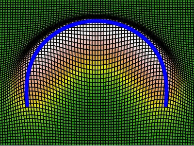
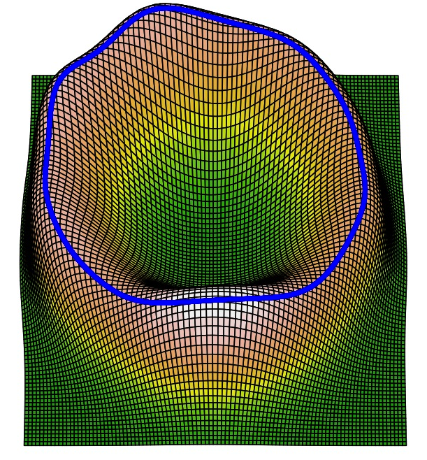
is positive, the ridges have the properties of filaments, i.e. smooth curve-like structures with high density (see Figure 1). Note that will include modes of the density which, in the context of cosmic filament detection, means that contains both filaments and galaxy clusters. Also note that density ridges are more general objects than the skeleton models proposed in Novikov et al. (2006); Sousbie et al. (2008) and the Spine method (Aragón-Calvo et al., 2010b). Essentially, when , density ridges are the same as skeletons.
Compared with other models, density ridges adapt information from both gradient and Hessian matrix of density. In contrast, MMF (Aragón-Calvo et al., 2007, 2010a), NEXUS and NEXUS+ (Cautun et al., 2013) only use the information of second derivatives (they define filaments as the regions with and ). DisPerSE models (Sousbie, 2011) define filaments as those gradient flows that start from saddle points and end up at local maximums, which utilize only the first derivatives.
An attractive feature for the density ridge model is that the statistical theory for consistently estimating the density ridge has been well-established (Genovese et al., 2014; Chen et al., 2014a, b). We also use N-body simulation to verify the convergence of density ridges when we subsample different number of galaxies (see Section 3.2).
2.2 SCMS: Filament Detection
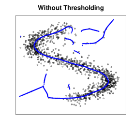
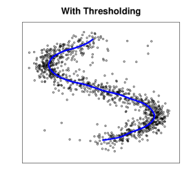


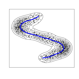
The algorithm consists of three steps described below and listed in Algorithm 1. The first is to estimate the underlying density function given , the observed locations of galaxies. We use the standard kernel density estimator (see e.g. Wasserman 2006):
| (4) |
where is the smoothing kernel (e.g. a Gaussian), is the Euclidean distance between the point and the galaxy location , and is the smoothing bandwidth (the selection of which is discussed in Appendix A).
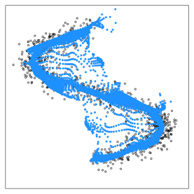
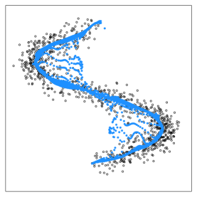
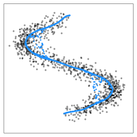
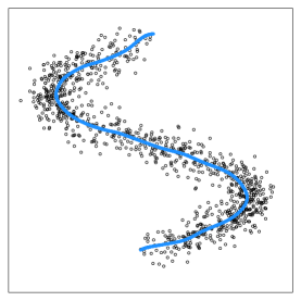
In the second step, we denoise by applying a threshold to the estimated density function to eliminate the effect that galaxies in low-probability density regions, i.e. where , would have on filament estimation. How one selects is also discussed in Appendix A. The denoising step is not part of the original SCMS algorithm but is important to increase its statistical power in low-density regions (see Figure 3. We note that a thresholding step is included in several filament-detection algorithms, including those of e.g. Novikov et al. (2006) and Sousbie (2011).
For the final step, given a set of galaxies in high-density regions, we apply the original version of the SCMS (Ozertem & Erdogmus, 2011) to detect filamentary structures. Given a point on a defined, uniform mesh, SCMS moves it according to an “estimated projected gradient" given by
| (5) |
where are estimates of the quantities that we define above in Section 2.1. One may view this procedure as estimating a ridge set by applying the Ridge operator to :
| (6) |
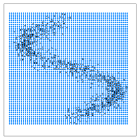
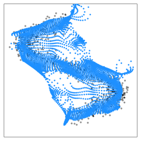
Essentially, is very similar to the filaments defined in Sousbie et al. (2008); Bond et al. (2010); Choi et al. (2010). Note that a putative filament is, in the context of this algorithm, a set of points and not a one-dimensional curve. In Step 4 of Algorithm 1, We further describe how we apply SCMS. In Figure 2, we illustrate the application of SCMS to uniform mesh of points, and in Figure 3 we demonstrate the importance of the thresholding step: the left and right panels show putative filaments detected without and with thresholding, respectively. We observe that thresholding greatly decreases the rate of false filament detection.
-
Step 1.
Compute the density estimator via equation (4).
-
Step 2.
Select a mesh of points. By default, we can take .
-
Step 3.
Thresholding: remove if . Let the remaining mesh points be denoted .
-
Step 4.
For each , perform the following subspace constrained mean shift until convergence:
-
Step 4-1.
For , compute
-
Step 4-2.
Compute the Hessian matrix
(7) -
Step 4-3.
Perform spectral decomposition on and compute , the eigenvectors corresponding to the smallest eigenvalues.
-
Step 4-4.
Update until convergence, where
(8) is called the mean shift vector.
-
Step 4-1.
2.3 SCMS: Filament Uncertainty Estimation
We quantify the uncertainty in the filament estimates produced by SCMS using the concept of local uncertainty (Chen et al., 2014a). The local uncertainty in an estimated filament at a point on the true filament is the expected distance between and the closest point to on . This is denoted by and is given by:
| (9) |
where and the notation denotes the expected value operator. is the radius of a local confidence ball that surrounds the point : the more uncertain the true location of the estimated filament, the larger the value of . We estimate , which is defined as a function of the unknown density field and the unknown filament set , by utilizing bootstrap resampling.
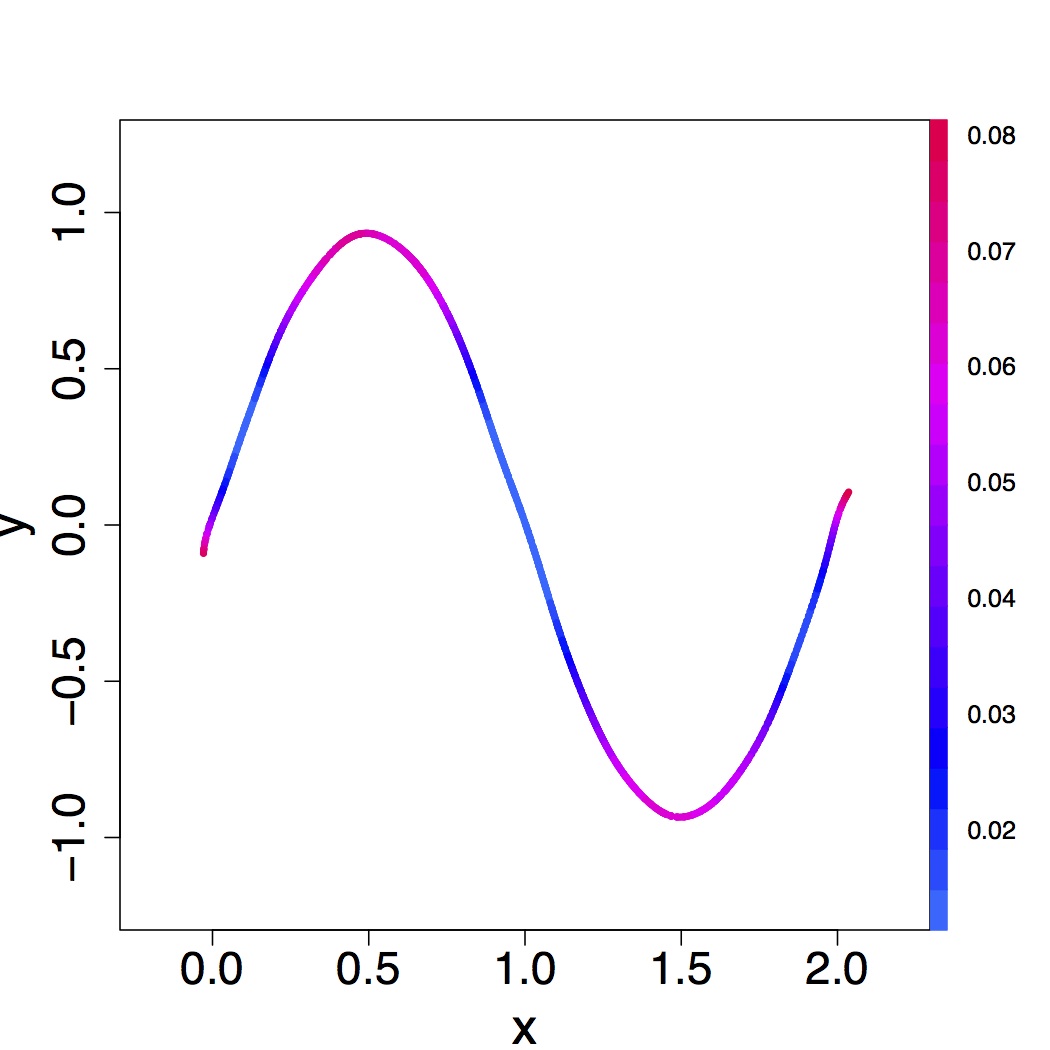
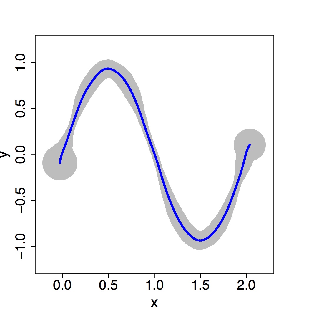
In this paper, we consider both the original version of bootstrap (Efron, 1979) and the smooth bootstrap. The smooth bootstrap (see e.g. Silverman & Young 1987) is a variant of the bootstrap that is useful in functional estimation problems in which the bootstrap sample is drawn from the estimated density instead of the original data. When the smoothing kernel is a bivariate Gaussian, we generate the smooth bootstrap sample via the following two steps:
-
1.
Generate the bootstrap sample.
-
2.
Add independent and identically distributed Gaussian noise with variance .
Unlike the bootstrap, the smooth bootstrap takes into account both the variance and the bias of filament estimation, but with less precision in variance estimation with respect to the bootstrap.
Assume we generate bootstrap samples, and each of them is denoted as , . For each bootstrap sample, say , we compute the density estimate , the ridge estimate , and the confidence ball radii for all . We estimate by adding the radius estimates in quadrature:
| (10) |
In Algorithm 2 we outline the computational steps that one must follow to derive .
Note that calculating the uncertainty measure is not part to the SCMS algorithm–we can detect filaments without using the uncertainty measure. However, this uncertainty measure is a feature that SCMS filaments have. This measure has a geometric interpretation and can be consistently estimated. See Chen et al. (2014a) for more involved discussion. Note that other filament finders do have have such a statistically consistent error measurement.
-
Step 1.
Perform SCMS on to detect filaments; denote the estimated filaments by .
-
Step 2.
Generate bootstrap samples: for .
-
Step 3.
For each bootstrap sample, apply SCMS which yields for .
-
Step 4.
For each , calculate , .
-
Step 5.
Compute .
2.4 SCMS: Boundary Bias
When computed with a kernel density estimator as in equation (4), SCMS filament estimates suffer from boundary bias within two bandwidths of the edge of the observation region. This is a systematic deviation from the true filament caused by the density estimator averaging over a region where no data can be observed, and it can degrade the confidence band coverage probabilities near the boundary. One remedy for boundary bias is to include additional data immediately outside of the region of interest. Including galaxies within of the boundaries eliminates most of the boundary bias, since very little of the volume under a bivariate Gaussian kernel lies beyond that point. If one cannot include additional data points outside the boundaries (for instance, due to overall survey limits), then one must be careful when interpreting filaments detected near the boundaries.
2.5 Filament Coverage
Here we introduce some useful geometric concepts about coverage. Given two sets and . The coverage of by is defined as
| (11) |
Note that when and are curves, they will contain infinite number of points. In this case, we will replace ‘number of points in’ by ‘the length of’. Similarly, we can define the coverage of by as .
Given two collections of filaments and , since and are curves so that they may not intersect each other in general so that the coverage is . Thus, instead of directly compute their coverage, we consider a flatten version of (and respectively). We define
| (12) |
as the r-flatten set of . Then we define the coverage of by as a function of as
| (13) |
Similarly, we can define . The two functions and contain information about the similarity between and .
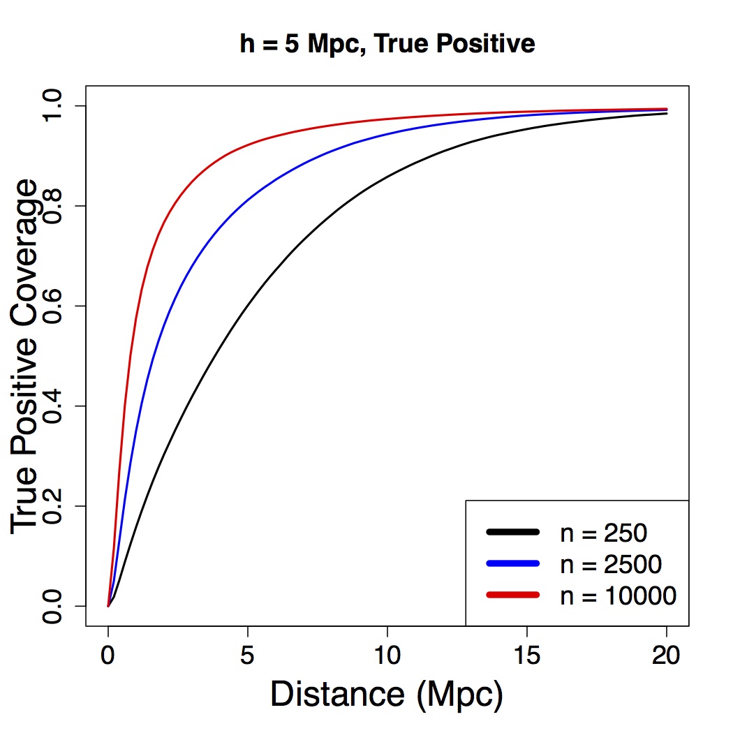
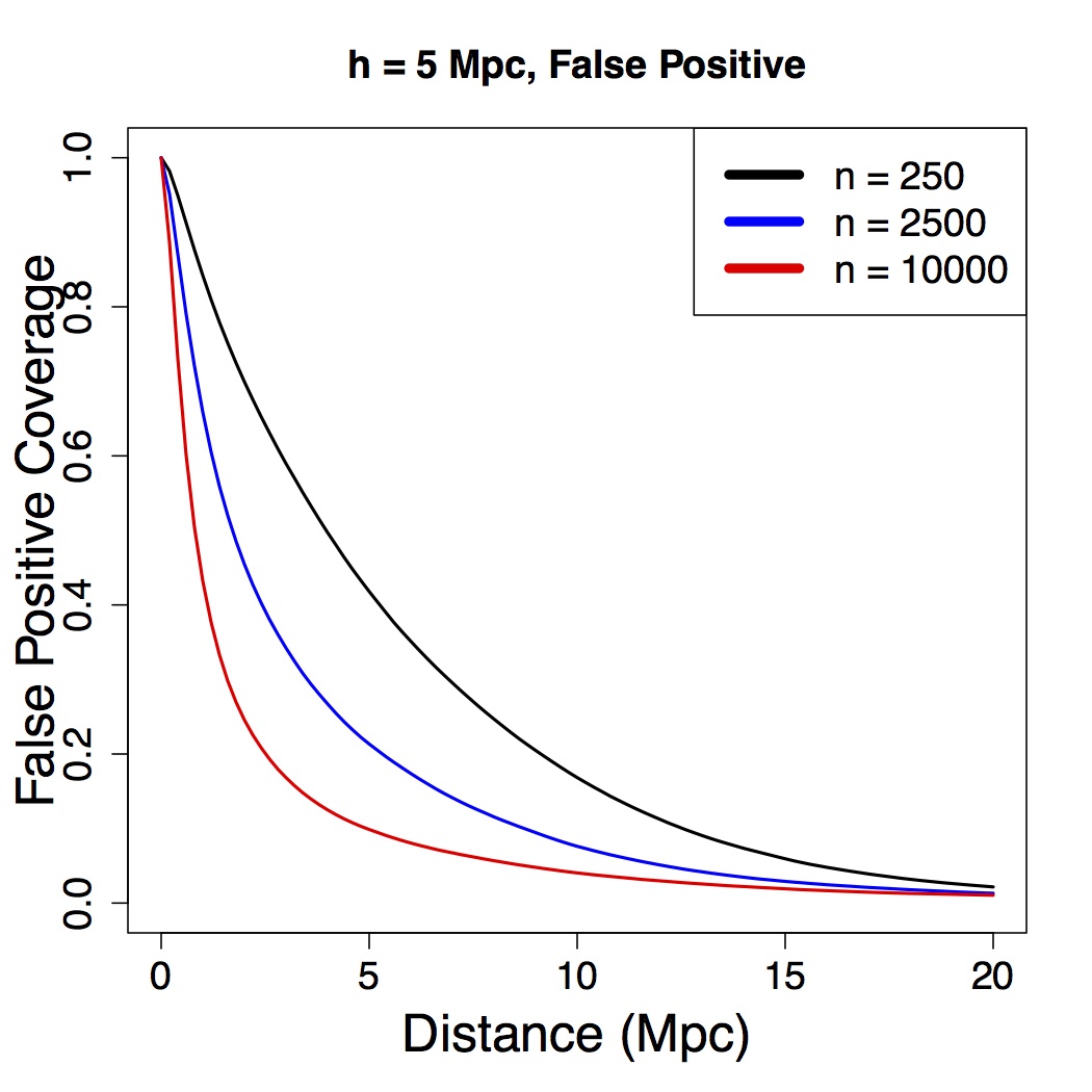
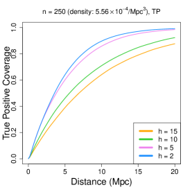
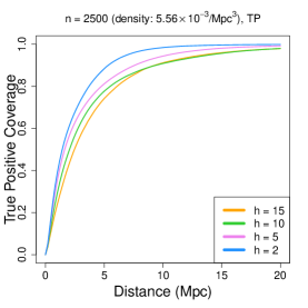
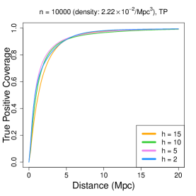
In simulation, we are able to define true filaments, say , and we will have an estimate filament, denoted as . Then we call the quantity the true positive coverage (ratio of true filaments being covered by estimated filaments) and we call the false positive coverage ( is the ratio of estimated filament being covered by truth so that 1 minus this ratio is the ratio of false positive). See Figure 9 for an example of true positive and false positive coverage.
Combining the uncertainty measures and the coverage, we can study the properties of the uncertainty band.. An uncertainty band for a detected filament is simply the union of the confidence balls computed for each point on the filament, i.e.
| (14) |
where represents the set of points within a ball centered at and with radius . Denote the region within the uncertainty band as . The coverage for is then
| (15) | ||||
One can think of as the true positive coverage using a set . For instance, if , then on average, 80% of the points on any given true filament lie within its associated uncertainty band, and 20% lie outside the band. This interpretation of coverage differs from the standard interpretation of confidence band coverage, thus motivating our use of the term “uncertainty band" instead of “confidence band." Figure 10 gives examples of the coverage for uncertainty bands with and and 2500. As we observe in Figure 10, the coverage percentage depends sensitively on the sample size ; thus, we cannot provide simple rules for converting uncertainty bands to coverage percentages.
3 Subspace Constrained Mean Shift: Applications
3.1 Voronoi Dataset
To show the effectiveness of capturing filaments, we compare the SCMS filaments (density ridges) to the filaments in the Voronoi model. The Voronoi model (van de Weygaert, 1994) applies Voronoi tessellation to compute a density estimate for galaxies as well as the curvature of that estimate. Given a curvature estimate, the Voronoi method assigns a class label to each galaxy, indicating the type of large-scale structure to which to associate the galaxy. There are four possible classes: cluster, filament, wall, and void.
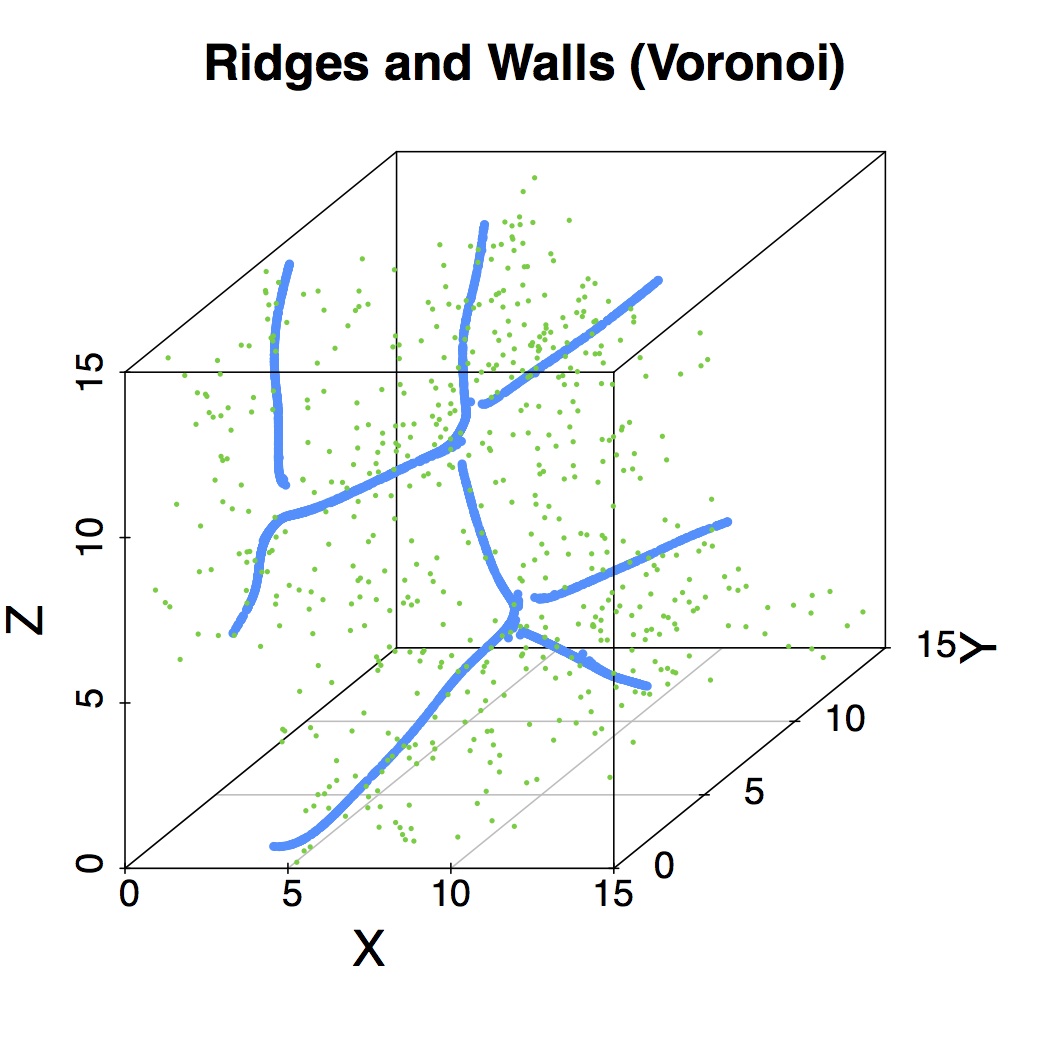
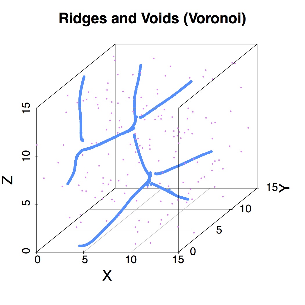
We use the SCMS algorithm to analyze a simulated dataset ( galaxies, each with a class label, that span a Mpc3 box) generated with the Voronoi model (M. A. Aragón-Calvo, private communication). Figure 6 shows a comparison between our density ridges (blue curves) and galaxies with different class labels (brown: cluster; red: filament; green: wall; pink: void). The two methods generate remarkably similar results: Voronoi clusters (i.e. galaxies labeled cluster) occur at the intersection points of density ridges; Voronoi filaments surround the density ridges; and Voronoi walls span surfaces on which the density ridges lay.
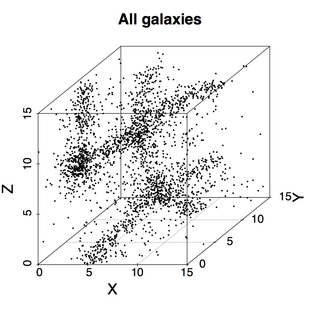
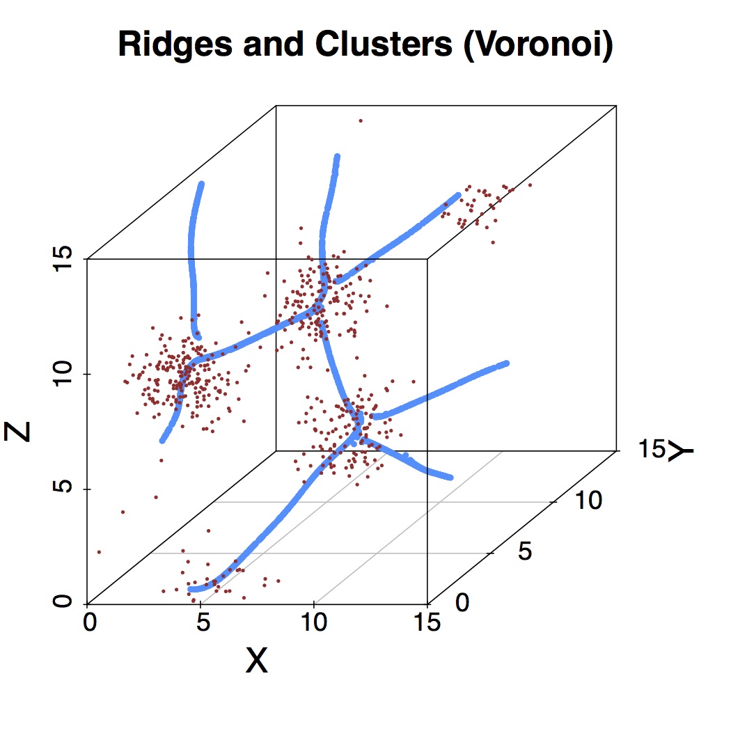
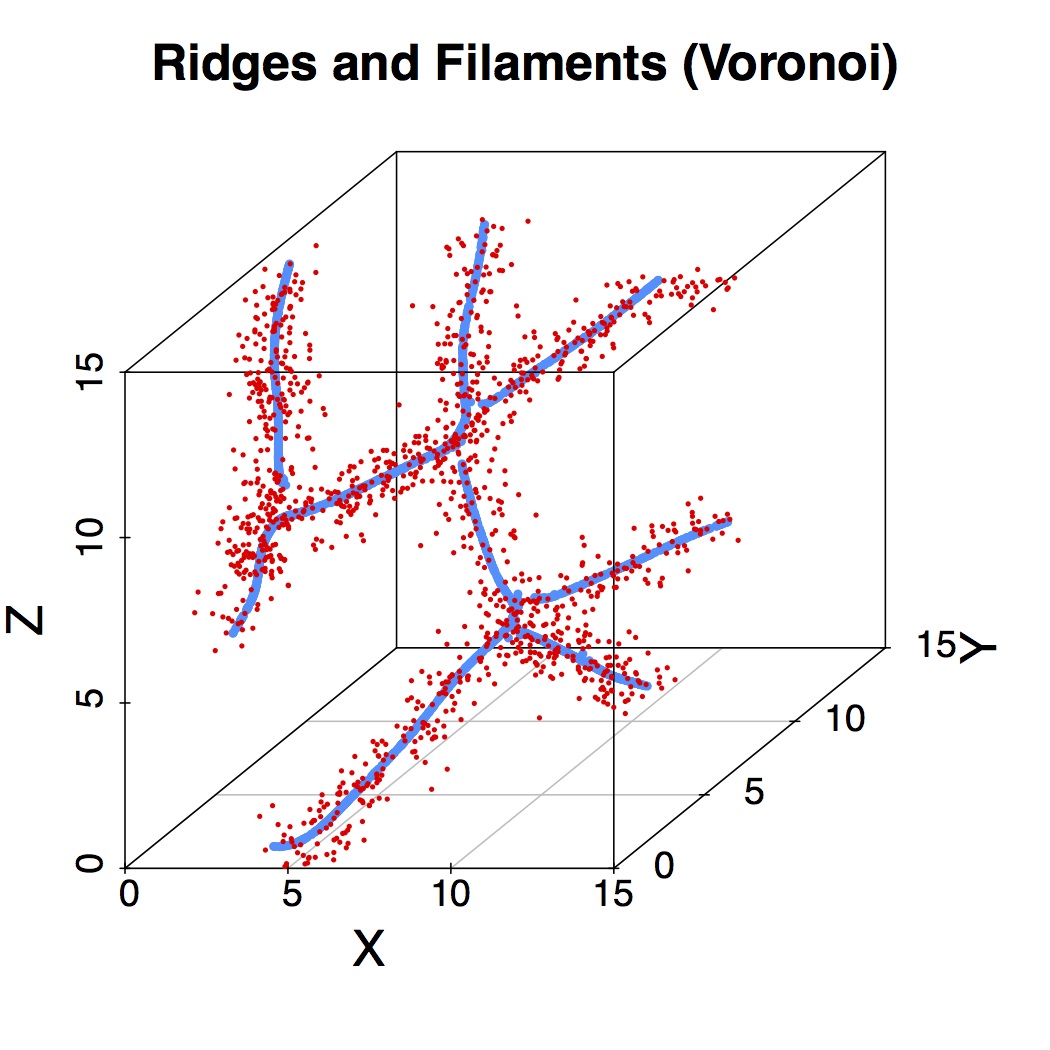
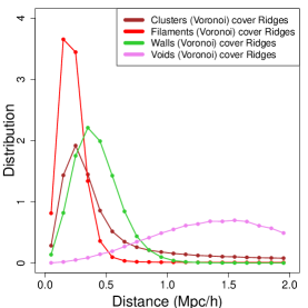
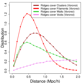
To further quantify the association between density ridges and each Voronoi model class, we study their projection distances onto each other. Note that the distribution of projection distances is related to filament coverage; further discussion of this may be found in Chen et al. (2015). Figure 7 displays the distributions of projection distances. In both panels, we see that the distribution for ridges versus the Voronoi filaments peaks at distances 1 Mpc This indicates that the density ridges and the Voronoi filaments are very similar. On the other hand, the projection distances from the density ridges increases as we consider clusters, walls, and voids; the distributions exhibit increasing positive skewness.
3.2 P3M N-body Simulation
To further demonstrate the efficacy of SCMS, we apply it to P3M N-body simulations from Trac et al. (2015), which assume a CDM cosmology with , , , , and . Each side of the simulation box is of length 1 Gpc/h, and each contains particles.
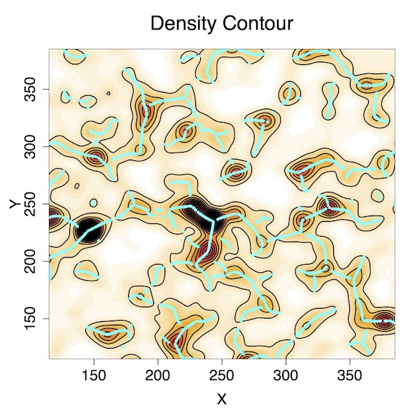
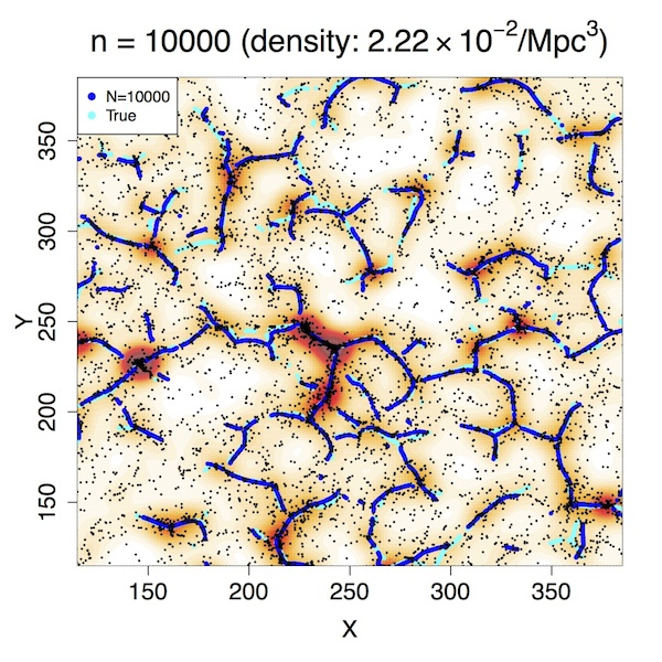
In Figure 8, we demonstrate that, as sample size increases, SCMS outputs filament estimates that are closer to the true filaments (defined by the true density function); the uncertainty measures capture SCMS errors due to the sampling variability. We take a slice of the full simulation data ( Mpc/h and Mpc/h) and smooth the data with smoothing bandwidth (recommended by the selection rule in Appendix A with ) to get the density function and the filaments (cyan curves). Figure 8(a) shows a contour plot for the density function. The original sliced data contains points (gray dots). We downsample to get three different subsamples; each contains particles. For each subsample (black dots), we apply SCMS to detect filaments (blue curves). Note that the convergence phenomena of Figure 8 are further quantified by the true positive and false positive coverage plot in Figure 9.
Note that the sparsest subsample has a galaxy number density Mpc-3 which is similar to the number density observed in SDSS CMASS data ( Mpc-3). The future survey Wide-Field Infrared Survey Telescope (WFIRST),111 http://wfirst.gsfc.nasa.gov/ a NASA mission with science objectives in exoplanet exploration, dark energy research and galactic and extragalactic surveys, will observe a number density similar to the subsample ( Mpc-3).
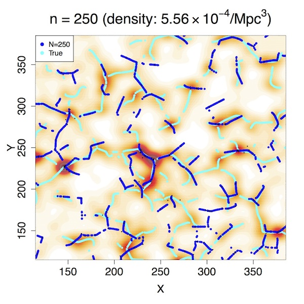
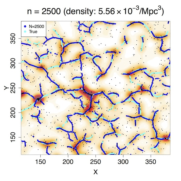
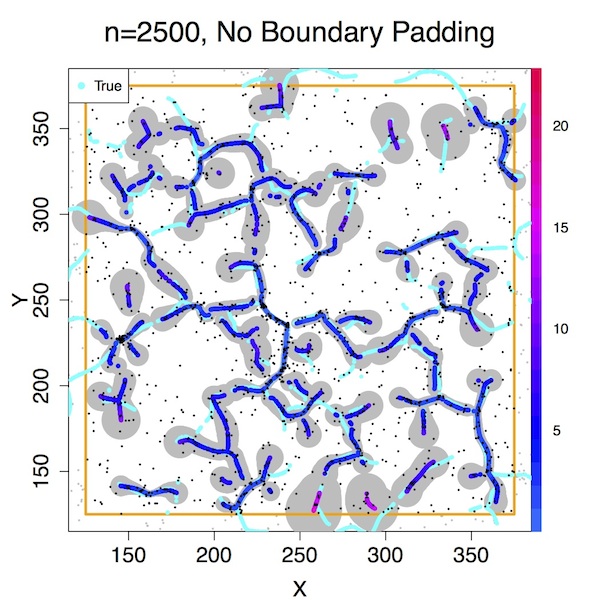
We show the uncertainty measures and filament coverage for in Figure 10. We plot filament coverage for confidence regions for in Figure 10(a), where and , and where is estimated by both the bootstrap (BT) and the smooth bootstrap (SB). This range contains sample sizes that are in line with both CMASS ( 250) and WFIRST ( 2500) data. We observe that filament coverage is, as noted above, sensitive to the sample size and that the smooth bootstrap provides considerably more conservative confidence bands, particularly for . The gray regions displayed in Figure 10(b) are the smooth bootstrap confidence regions , which we estimate contain 85% of the true filaments (cyan curves).
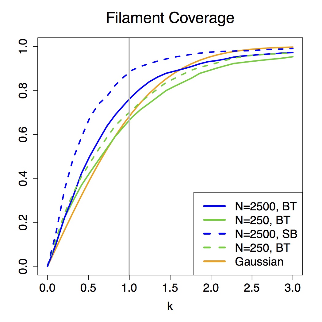
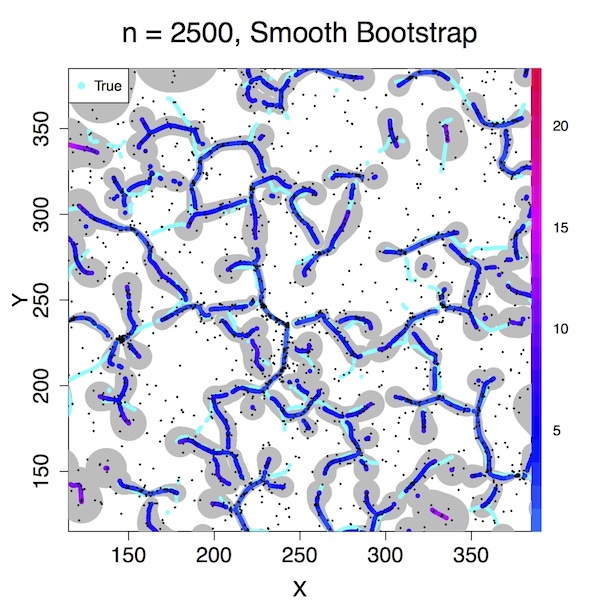
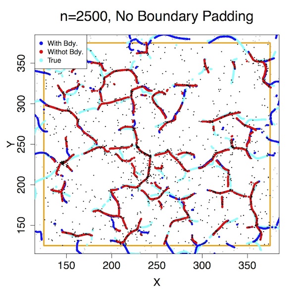
Figure 11 illustrates the effect of boundary bias in the subsample by comparing the estimates and uncertainties with padded and unpadded data near the boundary. Panels (a) and (b) show the boundary bias. Note that the red curves are filaments estimated by using only points within the boundary (given by the orange rectangle). The blue curves are filaments detected by SCMS with boundary points (i.e. points outside the orange rectangle). As can be seen, the estimation of filaments without boundary data (red curves) becomes more inaccurate as we approach the boundary. The boundary bias occurs for filaments with distances less than 10 Mpc/h ( times smoothing parameter ) to the boundaries. The uncertainty measures also show the influence of boundary bias. Figure 11(c) and 11(d) exhibit the uncertainty measures for filaments estimated with and without boundary points. As expected, the uncertainty measures in panel (d) increase as we move close to the boundary.


3.3 Sloan Digital Sky Survey
3.3.1 Data
We further demonstrate the efficacy of SCMS by applying it to data from Data Release 12 (Alam et al., 2015) of the Sloan Digital Sky Survey (SDSS; York et al., 2000). Together, SDSS I, II (Abazajian et al., 2009), and III (Eisenstein et al., 2011) used a drift-scanning mosaic CCD camera (Gunn et al., 1998) to image over one third of the sky ( square degrees) in five photometric bandpasses (Fukugita et al., 1996; Smith et al., 2002; Doi et al., 2010) to a limiting magnitude of , using the dedicated 2.5-m Sloan Telescope (Gunn et al., 2006) located at Apache Point Observatory in New Mexico. The imaging data were processed through a series of pipelines that perform astrometric calibration (Pier et al., 2003), photometric reduction (Lupton et al., 2001), and photometric calibration (Padmanabhan et al., 2008). All of the imaging was reprocessed as part of SDSS Data Release 8 (2011ApJS..193…29A; Aihara et al. 2011).
The Baryon Oscillation Spectroscopic Survey (BOSS) has obtained spectra and redshifts for 1.35 million galaxies over a footprint covering square degrees. These galaxies are selected from the SDSS 2011ApJS..193…29A imaging and are being observed together with quasars and approximately ancillary targets. The targets are assigned to tiles of diameter using a 2003AJ….125.2276B algorithm that is adaptive to the density of targets on the sky (Blanton et al., 2003). Spectra are obtained using the double-armed BOSS spectrographs (Smee et al., 2013). Each observation is performed in a series of -second exposures, integrating until a minimum signal-to-noise ratio is achieved for the faint galaxy targets. This ensures a homogeneous data set with a high redshift completeness of more than percent over the full survey footprint. Redshifts are extracted from the spectra using the methods described in Bolton et al. (2012). A summary of the survey design appears in Eisenstein et al. (2011), and a full description is provided in Dawson et al. (2013).
BOSS selects two classes of galaxies to be targeted for spectroscopy using SDSS 2011ApJS..193…29A imaging: ‘LOWZ’ and ‘CMASS’ (we refer the reader to Anderson et al. (2014) for further description of these classes). For the LOWZ sample, the effective redshift is , slightly lower than that of the SDSS-II luminous red galaxies (LRGs) as we place a redshift cut . The CMASS selection yields a sample with a median redshift and a stellar mass that peaks at (Maraston et al., 2013). Most CMASS targets are central galaxies residing in dark matter haloes of mass .
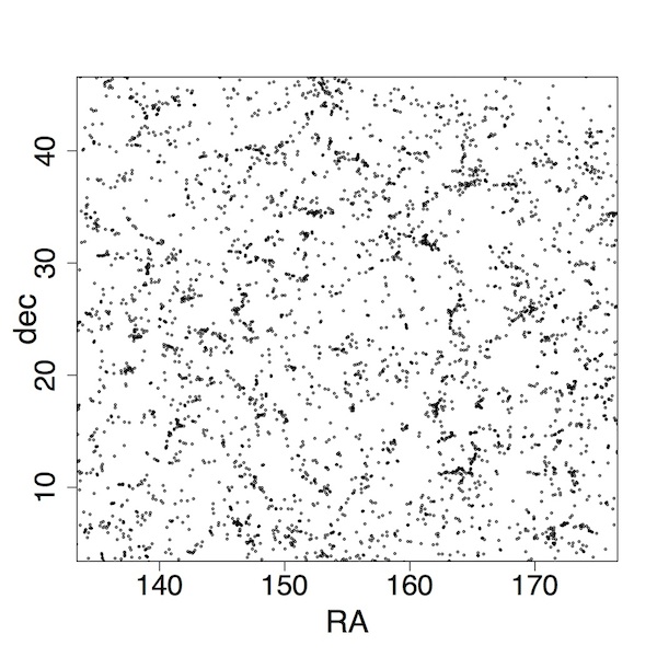
We test SCMS using two slices of data: at low and high redshift. The low- dataset comprises galaxies in the volume
while the high- dataset lies in the volume
and contains galaxies. Both samples have a very thin redshift range (the corresponding comoving distance is around Mpc) so that their constituent galaxies may be viewed as lying on a two-dimensional surface with coordinates (RA,).
There are two principal reasons for our choice to perform a two-dimensional analysis of the SDSS data. The first is that there is too large a change in the number density of detected galaxies over the SDSS redshift range. The SCMS algorithm incorporates kernel density estimation to locate density ridges, and KDE requires a fixed smoothing parameter . However, in low-density regions, should be large to obtain reliable results, while in high-density regions, has to be small so as to not oversmooth the point cloud. The second reason is that when , the number density is very low, and performing a three-dimensional analysis will produce results with large statistical errors due to the small sample size. Lower-dimensional analyses result in decreased statistical error; see e.g. Wasserman 2006.
3.3.2 Results
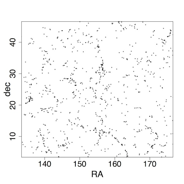
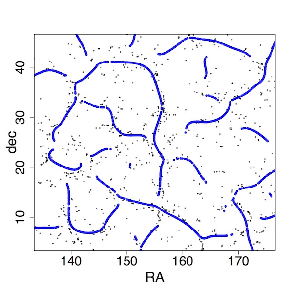
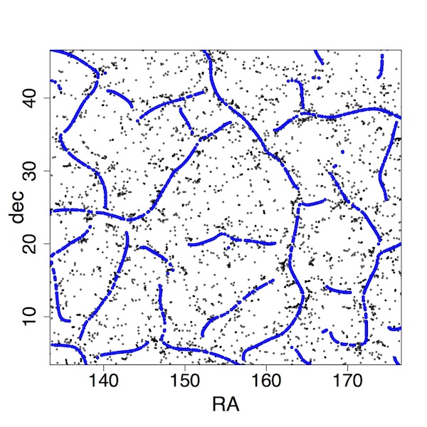
We apply SCMS to the low- data with smoothing bandwidth (41.8 Mpc) and threshold level ; we display our results in Figure 12. For the high- data, and are (71.1 Mpc) and , respectively; we display our results in Figure 13. Note that we have included additional galaxies within degrees of our selected window to mitigate boundary bias.
As can be seen in Figures 12 and 13, SCMS filament estimates capture high density regions and they exhibit one-dimensional, nearly connected structures. In addition, SCMS yields smooth filaments; most filament estimators do not output such smooth structures (cf. Stoica et al., 2007; Stoica et al., 2005; Sousbie, 2011; Aanjaneya et al., 2012; Lecci et al., 2013). We note that the filaments detected by SCMS will not actually connect with each other; points on merging filaments have eigengap (equation 3) that asymptote toward , making the density ridge ill-defined since the first and second eigenvalues become equal. We note that in both figures there are possibly spurious filaments; for instance, in Figure 12, at (RA,) and , we see filaments that are associated with a relatively small number of galaxies. As we demonstrate below, these putative filaments have higher estimates of uncertainty.
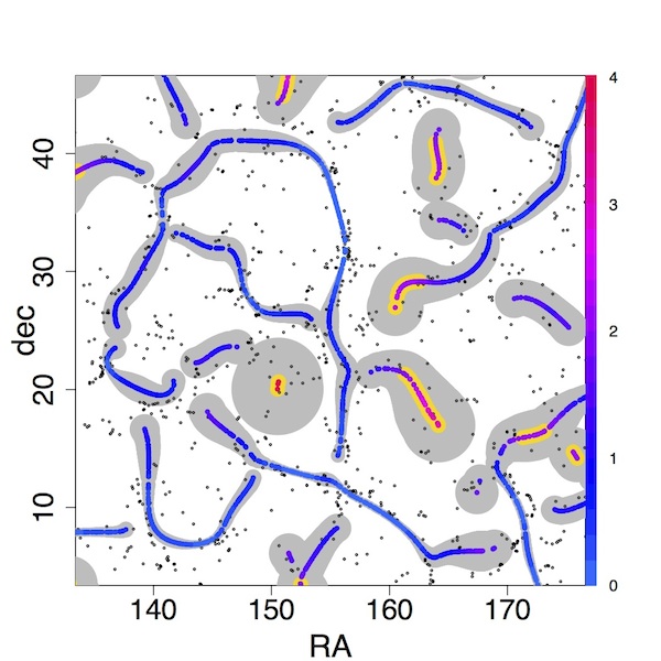
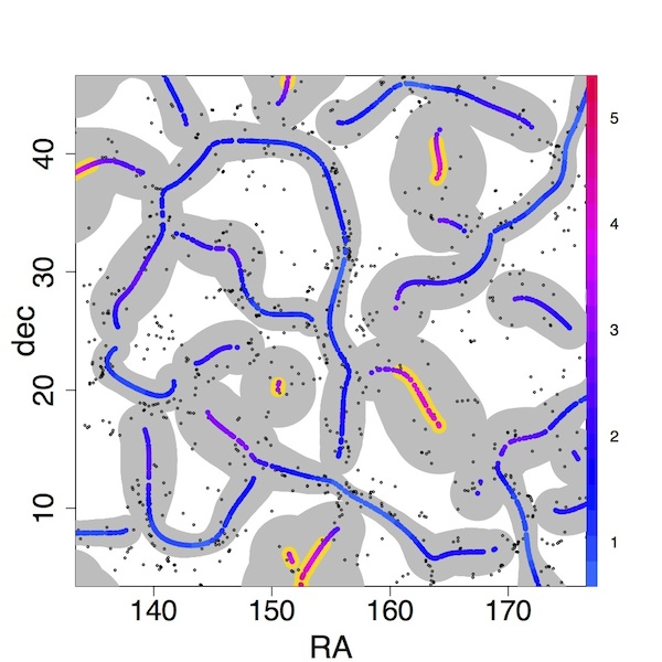
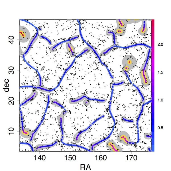
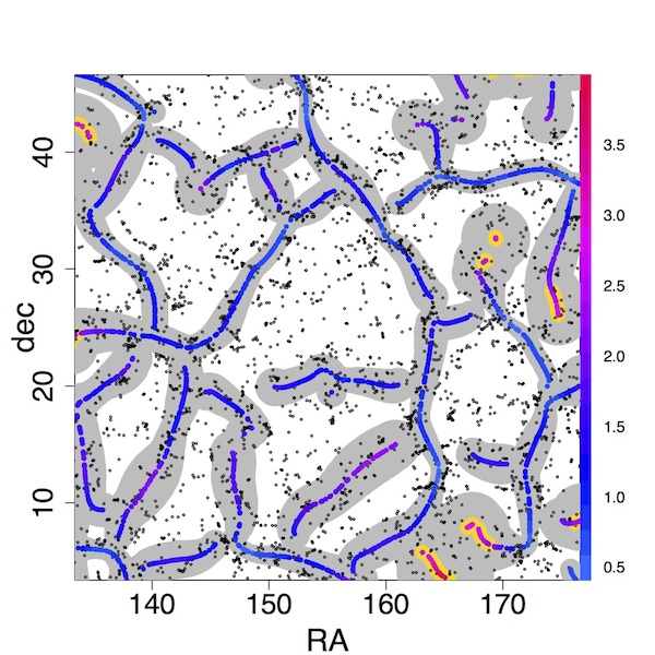
We derive the uncertainties for the filament estimators as described in Section 2.3 from the two test datasets; the results for low- and high- samples are given in Figures 14 and 15, respectively. We visualize local uncertainty using color, where red indicates locations where the filamentary structure is highly uncertain. We also display uncertainty regions as bands of varying width (shown in gray) centered on the filaments. Our simulation study in Section 3.2 indicates that the filament coverage for the regions in Figures 14(a) and 15(a) is , while that in Figures 14(b) and 15(b), is . We find that the overall structure for filaments in the high- dataset is more stable than for the low- data, due to the significantly larger size of the high- dataset; as shown in Figure 8, sample size plays a crucial role in determining the size of the uncertainty regions associated with SCMS filament estimates.
As can be inferred from Figures 14 and 15, our measures of local uncertainty provide useful information to determine the quality of filament detections. We declare a point to be ‘unstable’ if
| (16) |
where is the mean of uncertainty over all filament points and is the root mean square of uncertainty. Namely, if the local uncertainty at is too large, this point is not stable. The constant comes from the width of confidence interval for a Gaussian distribution. For instance the two filaments at (RA,) and in Figure 12 appear by eye to be spurious, given the relative lack of galaxies in their vicinity. Based on the uncertainty measures and our stability test (16), these filaments are declared as unstable (yellow color in Figure 14).
3.3.3 Test Data: Comparison to redMaPPer Clusters
As one last demonstration of the efficacy of SCMS, we examine the consistency between our filament maps and the galaxy clusters in the redMaPPer catalog (Rykoff et al., 2014; Rozo & Rykoff, 2014; Rozo et al., 2015). We make this comparison within the window
and within annuli of width from to (a range that includes galaxy clusters with spectroscopically determined redshifts, or of the redMaPPer sample). Note that we also include SDSS DR7 main sample galaxy from NYU VAGC (Blanton et al., 2005; Padmanabhan et al., 2008; Adelman-McCarthy et al., 2008) to detect filaments for low redshift regions (). We slice the data primarily for computational efficiency, since SCMS is an algorithm, but slicing has the ancillary benefit of simplifying visualization. In total we examine slices, each of which contains galaxy clusters. Within each slice, we determine optimal values of and using the criteria described in Appendix A.
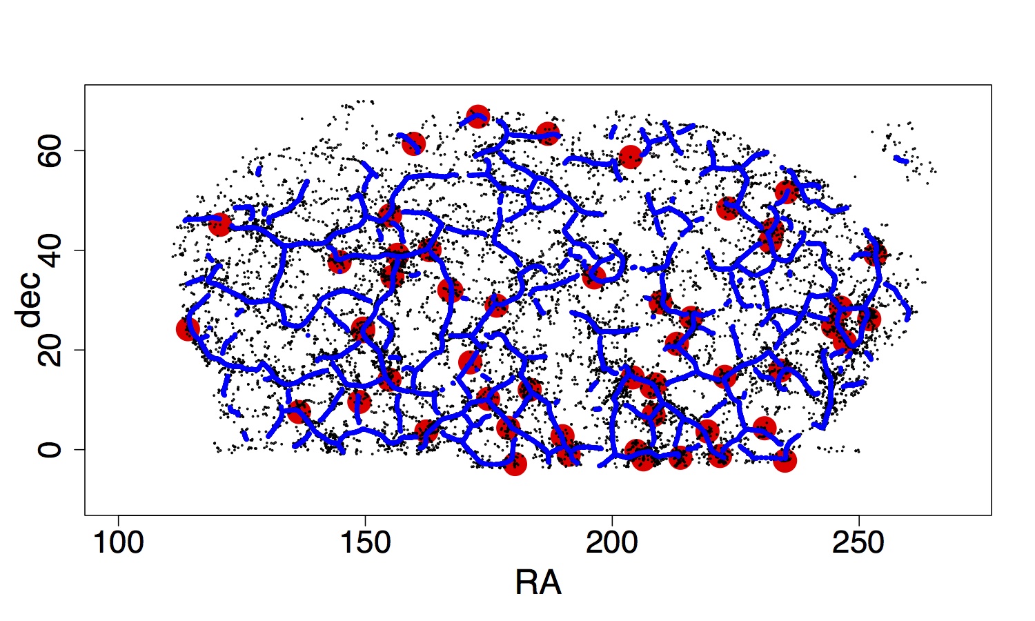
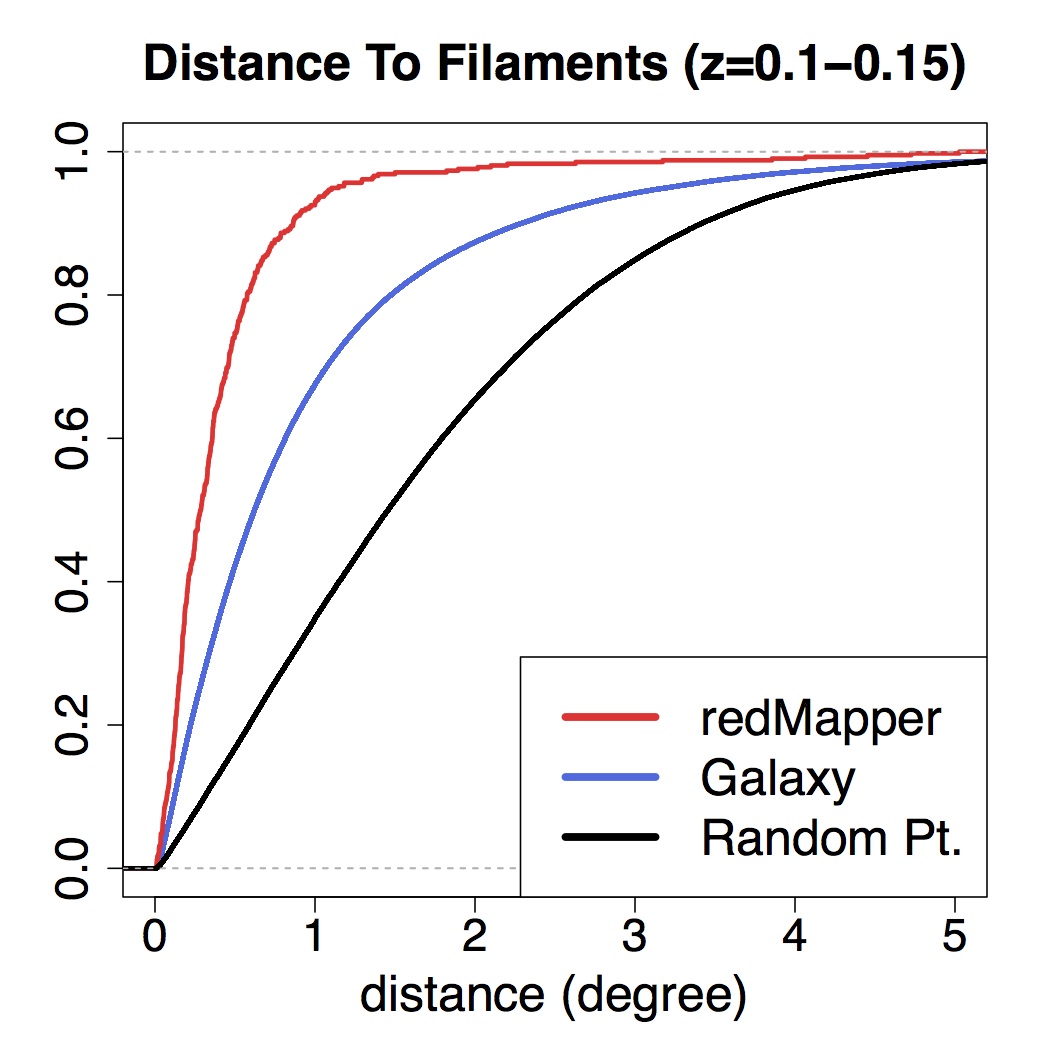
In Figure 16, we display SCMS-detected filaments along with redMaPPer clusters (in red). As can be seen, nearly all galaxy clusters are associated with detected filaments. Qualitatively similar results hold for all other slices. To quantify the association of galaxy clusters and filaments, we compare the distance to filaments for three types of objects: galaxy clusters, galaxies and randomly generated points within the regions where galaxies are observed. We divide the whole redshift range evenly into sub-regions (each sub-region contains 10 slices); within each sub-region we compute distance statistics. Ideally, galaxy clusters should be systematically closer to filaments than galaxies are, and both galaxies and galaxy clusters should be far closer to filaments than randomly generated points. Figure 17 and Table 1 confirm this hypothesis. Figure 17 shows the cumulative distribution for these distance statistics. For a collection of values , the cumulative distribution function (CDF) is a non-decreasing function ranging from to defined as
| (17) |
Both galaxies (blue curves) and galaxy clusters (red curves) tend to be much closer to the filaments than random points; this suggests that galaxies and galaxy clusters are indeed concentrated around the detected filaments. When we compare galaxies and clusters, we observe that galaxy clusters are much more right-skewed in the CDF plot for every redshift sub-region. That is, galaxy clusters tend to distribute around low-distance-to-filament regions compared to a random galaxy. We conduct the two-sample, one-sided KS test (Stephens, 1974), which compares the distributions of distance statistics for galaxy clusters and randomly generated points, for all eight sub-regions. Table 1 shows the -values, a statistical quantity measuring the significance of observations, for the eight KS tests that we carry out. A smaller p-value indicates stronger evidence for clusters being closer to a filament than galaxies. Typically, we declare significance as p-value being less than . We observe an increasing trend in -value as the redshift increases, due to the decrease in the number density of galaxies along the line of sight. The sharp reversal in this trend at the last sub-region () is due to the large size of the CMASS sample at : the number density of galaxies in our sample actually increases from .
Note that in Figure 16, many clusters appear to be located near the intersections of filaments. However, we do not construct a statistics to summarize this phenomena since defining the intersections of filaments detected by SCMS is a non-trivial problem. The main difficulty is due to the ‘gap’ between filaments; the SCMS filaments will not intersect each other but with a small gap. This gap can be explained by the model of density ridges. In the density ridges model, we require the eigengap (recall equation (3)) to ensure the properties of filaments. Therefore, when one ridge merges with another, the eigengap vanishes at some point (i.e. ). This leaves a small gap between one ridge and another.
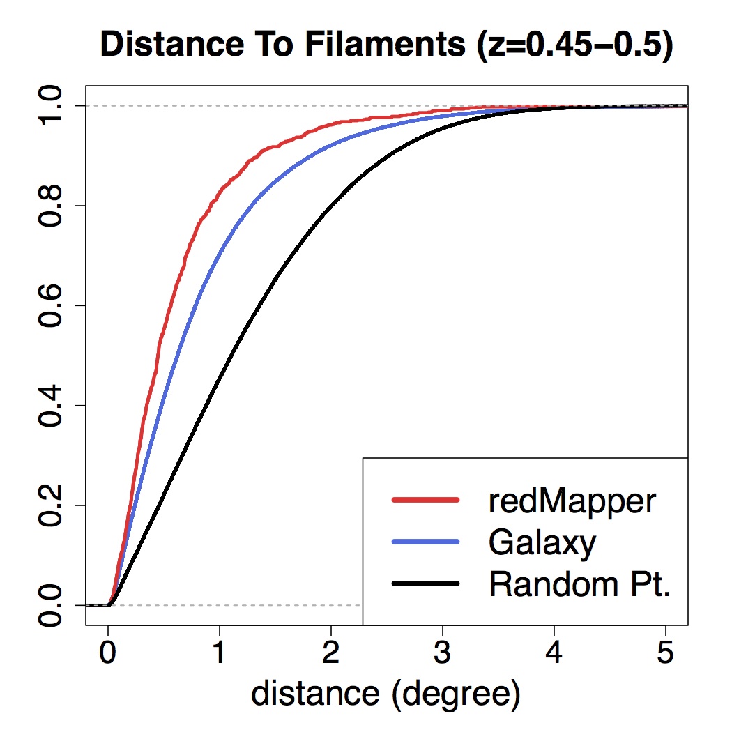
| Redshift | -value | Redshift | -value |
|---|---|---|---|
| 0.100-0.150 | 0.300-0.350 | ||
| 0.150-0.200 | 0.350-0.400 | ||
| 0.200-0.250 | 0.400-0.450 | ||
| 0.250-0.300 | 0.450-0.500 |
4 Summary and Discussion
In this paper, we demonstrate how one may apply the Subspace Constrained Mean Shift (SCMS) algorithm of Ozertem & Erdogmus (2011) to uncover filamentary structure in galaxy point cloud data. The density ridge model behind the SCMS algorithm ensures that galaxies will concentrate around detected filaments. In addition, we introduce an uncertainty measure for detected filaments that is based on the bootstrap, allowing us to study the significance of these filaments.
In §3 we first show that the SCMS filaments are very similar to the Voronoi filaments. Then we demonstrate the efficacy of our SCMS-based filament-finding algorithm by applying it both to P3M N-body simulation output and to SDSS DR 12 data (including the NYU main sample galaxy, LOWZ and CMASS datasets). By applying SCMS to simulated data, we are able to estimate the coverage of our bootstrap-generated uncertainty bands, i.e. the fraction of any one true filament that lies within its associated band (see Figure 10). We find that the coverage depends sensitively on the number of galaxies in an analyzed sample, with the smooth bootstrap algorithm generating more conservative uncertainty bands with 1 coverage 0.6-0.8 (cf. 0.683 for a 1 confidence band) for galaxy number densities 5 10-4 - 5 10-3 (densities observed/to be observed by SDSS CMASS and WFIRST, respectively).
In Figures 12-15, we show the results of applying the SCMS algorithm to SDSS spectroscopically observed galaxies in the redshift slices 0.235 0.240 and 0.530 0.535, respectively. To test the hypothesis that our estimated filaments are associated with real filamentary structures, we compare the distances between filaments and redMaPPer galaxy clusters, random field galaxies, and random points in the galaxy field. By using the one-sided, two-sample KS test, we find that we can safely reject the null hypothesis that galaxy clusters and field galaxies reside at similar distances from filaments; the -values are (cf. the usual rejection criterion that ; see Table 1).
The SCMS algorithm models filaments as one-dimensional ridges that trace high-density regions within the point cloud; as such, SCMS may be grouped with other filament-modeling algorithms that use the eigenvalues and eigenvectors of the Hessian matrix associated with the point cloud density function, such as MMF (Aragón-Calvo et al., 2007, 2010a) and NEXUS/NEXUS+ (Cautun et al., 2013). However, in contrast to these methods, which output filament estimates as two-dimensional regions, SCMS filament estimates are smooth, one-dimensional curves; the filament orientations are well-defined. Also in contrast to these methods, we offer measures of uncertainty by augmenting the SCMS algorithm with bootstrap-based uncertainty estimation algorithms that allow one to e.g. place bands around putative filaments, whose relative sizes indicate uncertainty in filament location (as in e.g. Figure 5). We note that the segmentation-based DisPerSE algorithm of Sousbie (2011) uses the persistence ratio, a metric encapsulating the evolution of topological structure in the galaxy field, to define the significance of putative filaments, but not their spatial uncertainty. Finally, we compare SCMS filaments to those generated by the Spine (Aragón-Calvo et al., 2010b; Aragon-Calvo & Yang, 2014) and Skeleton (Novikov et al., 2006) algorithms. Both the Skeleton and Spine models look for ridges within a density field. However, the Skeleton model does not provide a means by which to compute density ridges. In contrast, the SCMS algorithm allows us to efficiently compute ridges of the field’s kernel density estimate. The Spine method outputs ridges as points on grids, so that resolution is an issue. On the other hand, the SCMS algorithm yields points that are on continuous curves (ridges), so there is no resolution issue to address.
We conclude by stating that one may extend the use of the SCMS algorithm beyond the analysis of galaxy point cloud data. For instance, Chen et al. (2014b) discuss how to apply the algorithm to pixelized image data; in particular, they modify the algorithm (calling it the weighted SCMS algorithm) to find intensity ridges caused by e.g. tidal tails. In addition, the authors also discuss how one would incorporate the mass of a galaxy to achieve a better estimate of the local density as well as of corresponding ridges.
Acknowledgments
We thank Hy Trac for providing the Nbody simulations and Rachel Mandelbaum for useful discussions. We also thank the referee Miguel A. Aragón-Calvo for useful comments and for providing the Voronoi dataset that we analyze in § 3.1. This work is supported in part by the Department of Energy under grant DESC0011114; YC is supported by DOE; SH is supported in part by DOE-ASC, NASA and NSF; CG is supported in part by DOE and NSF; LW is supported by NSF.
Funding for SDSS-III has been provided by the Alfred P. Sloan Foundation, the Participating Institutions, the National Science Foundation, and the U.S. Department of Energy Office of Science. The SDSS-III web site is http://www.sdss3.org/.
SDSS-III is managed by the Astrophysical Research Consortium for the Participating Institutions of the SDSS-III Collaboration including the University of Arizona, the Brazilian Participation Group, Brookhaven National Laboratory, Carnegie Mellon University, University of Florida, the French Participation Group, the German Participation Group, Harvard University, the Instituto de Astrofisica de Canarias, the Michigan State/Notre Dame/JINA Participation Group, Johns Hopkins University, Lawrence Berkeley National Laboratory, Max Planck Institute for Astrophysics, Max Planck Institute for Extraterrestrial Physics, New Mexico State University, New York University, Ohio State University, Pennsylvania State University, University of Portsmouth, Princeton University, the Spanish Participation Group, University of Tokyo, University of Utah, Vanderbilt University, University of Virginia, University of Washington, and Yale University.
Appendix A Parameter Selection
Our version of SCMS has two key parameters, the smoothing bandwidth and the threshold level . In this section we show how we select optimal values for each.
The smoothing bandwidth represents the amount by which we smooth the observed point cloud of galaxies when estimating . One can choose by applying prior knowledge or by letting adapt to the sample. There is a large body of literature on the choice of bandwidth, e.g. Sheather et al. (2004) and Chacón et al. (2011, 2013). Among all methods, we recommend choosing via
| (18) |
where is a constant that we discuss below, is the sample size, is the dimension (in our case ) and is the minimal value for the standard deviation along each coordinate. Note that the reference rule (18) will choose smaller values as the sample size increases.
If is , (18) corresponds to Silverman’s rule (Silverman, 1986). Silverman’s rule selects via minimizing the mean integrated error
| (19) |
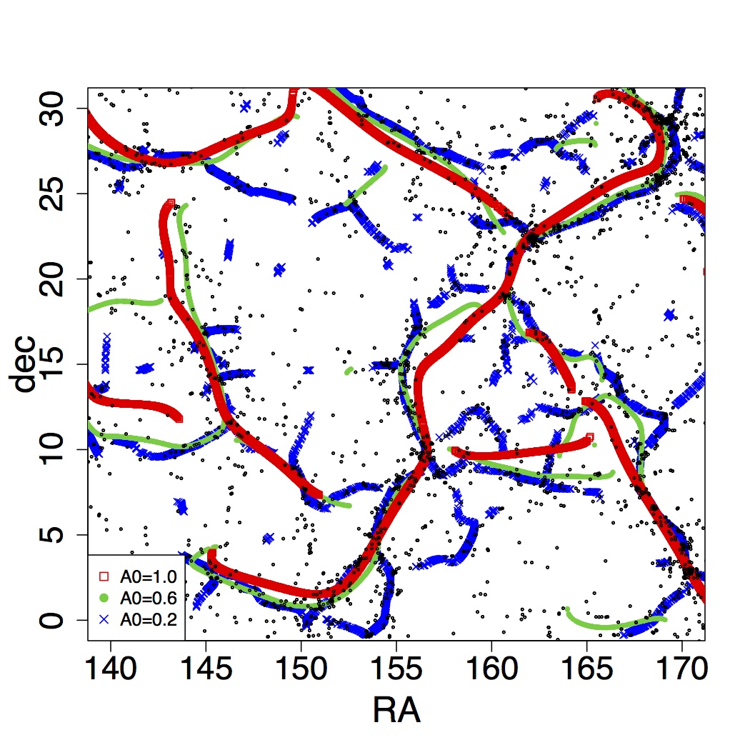
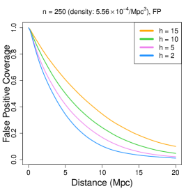
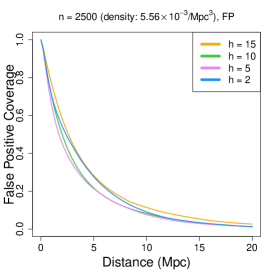
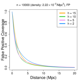
when is a Gaussian. When the data include filaments, is no longer Gaussian and must be optimized as a free parameter. A smaller yields more filaments in a given dataset but more spurious filaments as well. There is no general rule for selecting since the optimality criterion involves the unknown density . Figure 18 shows how varying affects the estimation of filamentary structures. Our results indicate that the optimal lies in the range . This is further confirmed by true positive and false positive coverage of N-body simulation (described in section 3.2) as shown in Figure 19. In N-body simulation, corresponds to Mpc (actual value is ) while corresponds to Mpc (actual value is ). Both values are better than being too large or too small (compared with Mpc and Mpc cases). In our analyses of SDSS data, we adopt the value .
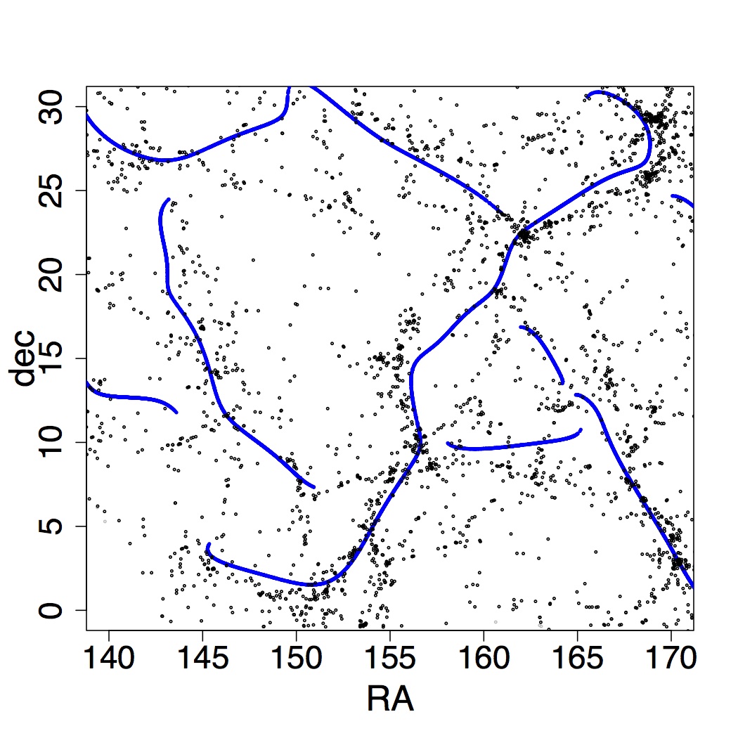
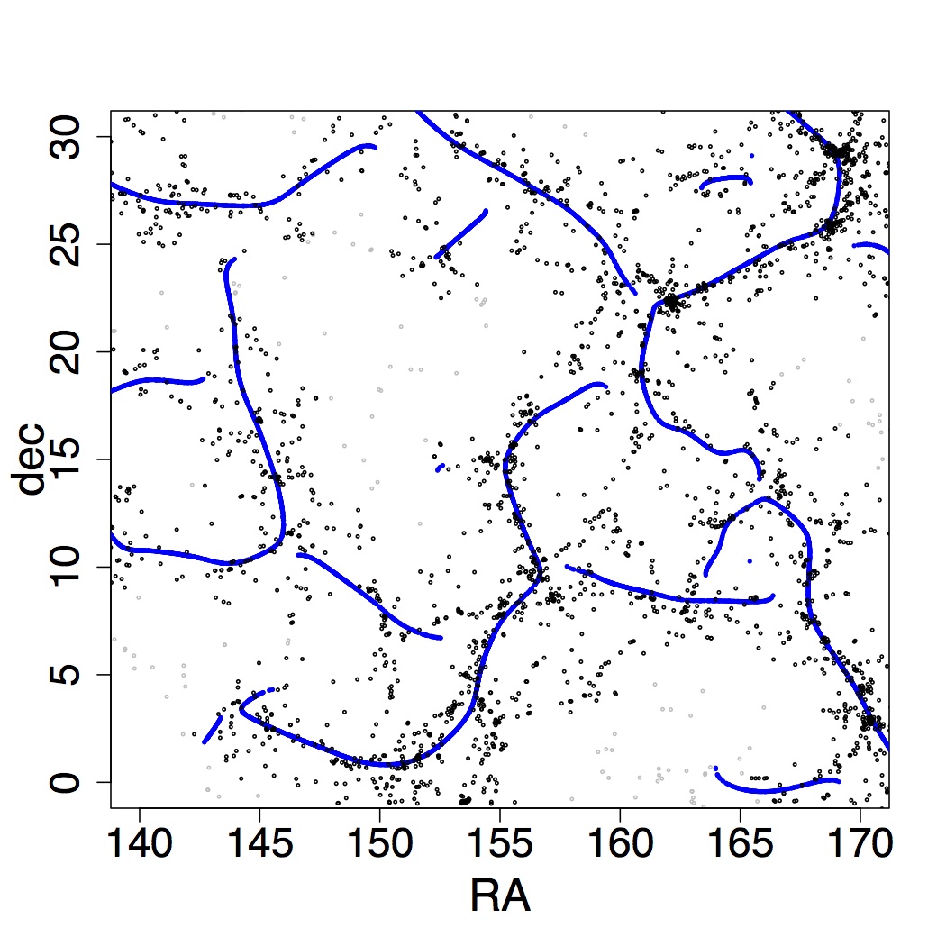
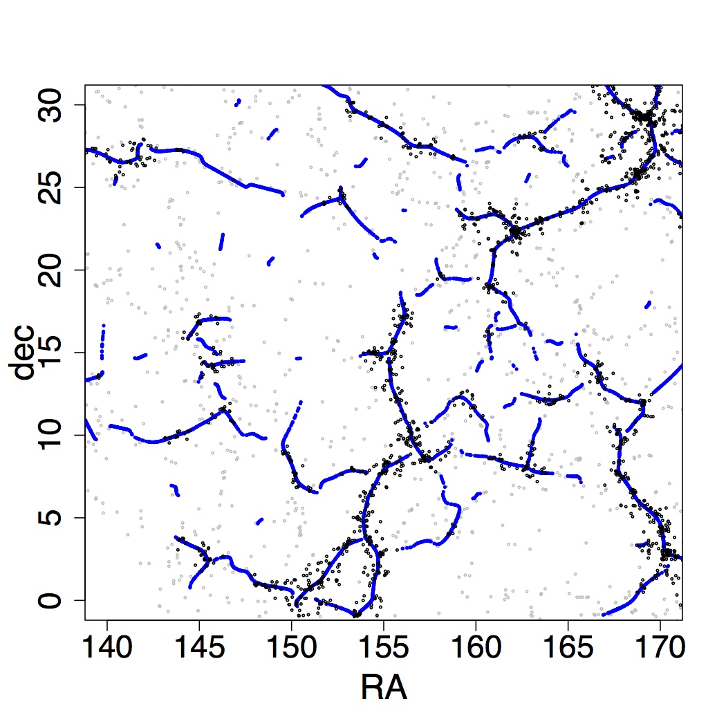
Thresholding stabilizes the ridge-finding process since random noise may cause small bumps in the estimated density field. However, if the threshold is set too high, we will remove useful information about the field. We recommend selecting the thresholding level according to the root mean square (RMS) in the density fluctuation:
| (20) |
where is the region we are interested in and is the average density in . Note that thresholding is also utilized by the MMF (Aragón-Calvo et al., 2010a) and NEXUS (Cautun et al., 2013) filament- (and galaxy cluster-) detection algorithms.
References
- Aanjaneya et al. (2012) Aanjaneya M., Chazal F., Chen D., Glisse M., Guibas L., Morozov D., 2012, International Journal of Computational Geometry and and Applications, 22, 305
- Abazajian et al. (2009) Abazajian K. N., et al., 2009, \apjs, 182, 543
- Adelman-McCarthy et al. (2008) Adelman-McCarthy J. K., et al., 2008, \apjs, 175, 297
- Aihara et al. (2011) Aihara H., et al., 2011, \apjs, 193, 29
- Alam et al. (2015) Alam S., et al., 2015, preprint, (arXiv:1501.00963)
- Anderson et al. (2014) Anderson L., et al., 2014, MNRAS, 439, 83
- Aragon-Calvo & Yang (2014) Aragon-Calvo M. A., Yang L. F., 2014, \mnras, 440, L46
- Aragón-Calvo et al. (2007) Aragón-Calvo M. A., Jones B. J. T., van de Weygaert R., van der Hulst J. M., 2007, A&A, 474, 315
- Aragón-Calvo et al. (2010a) Aragón-Calvo M. A., van de Weygaert R., Jones B. J. T., 2010a, \mnras, 408, 2163
- Aragón-Calvo et al. (2010b) Aragón-Calvo M. A., Platen E., van de Weygaert R., Szalay A. S., 2010b, \apj, 723, 364
- Blanton et al. (2003) Blanton M. R., Lin H., Lupton R. H., Maley F. M., Young N., Zehavi I., Loveday J., 2003, \aj, 125, 2276
- Blanton et al. (2005) Blanton M. R., et al., 2005, \aj, 129, 2562
- Bolton et al. (2012) Bolton A. S., et al., 2012, \aj, 144, 144
- Bond et al. (1996) Bond J. R., Kofman L., Pogosyan D., 1996, Nature, 380, 603
- Bond et al. (2010) Bond N. A., Strauss M. A., Cen R., 2010, \mnras, 409, 156
- Cautun et al. (2013) Cautun M., van de Weygaert R., Jones B. J. T., 2013, MNRAS, 429, 1286
- Cautun et al. (2014) Cautun M., van de Weygaert R., Jones B. J. T., Frenk C. S., 2014, MNRAS, 441, 2923
- Chacón et al. (2011) Chacón J. E., Duong T., Wand M., 2011, Statistica Sinica, 21
- Chacón et al. (2013) Chacón J. E., Duong T., et al., 2013, Electronic Journal of Statistics, 7, 499
- Chen et al. (2014a) Chen Y.-C., Genovese C. R., Wasserman L., 2014a, preprint, (arXiv:1406.5663)
- Chen et al. (2014b) Chen Y.-C., Genovese C. R., Wasserman L., 2014b, preprint, (arXiv:1406.1803)
- Chen et al. (2015) Chen Y.-C., Genovese C. R., Ho S., Wasserman L., 2015, preprint, (arXiv:1506.02278)
- Choi et al. (2010) Choi E., Bond N. A., Strauss M. A., Coil A. L., Davis M., Willmer C. N. A., 2010, \mnras, 406, 320
- Clampitt et al. (2014) Clampitt J., Jain B., Takada M., 2014, preprint, (arXiv:1402.3302)
- Codis et al. (2014) Codis S., Dubois Y., Pichon C., Devriendt J., Slyz A., 2014, preprint, (arXiv:1409.2838)
- Colberg et al. (2005) Colberg J. M., Krughoff K. S., Connolly A. J., 2005, MNRAS, 359, 272
- Dawson et al. (2013) Dawson K. S., et al., 2013, \aj, 145, 10
- Doi et al. (2010) Doi M., et al., 2010, \aj, 139, 1628
- Dolag et al. (2006) Dolag K., Meneghetti M., Moscardini L., Rasia E., Bonaldi A., 2006, \mnras, 370, 656
- Eberly (1996) Eberly D., 1996, Ridges in Image and Data Analysis. Springer
- Efron (1979) Efron B., 1979, Annals of Statistics, 7, 1
- Eisenstein et al. (2011) Eisenstein D. J., et al., 2011, \aj, 142, 72
- Forero-Romero et al. (2014) Forero-Romero J. E., Contreras S., Padilla N., 2014, MNRAS, 443, 1090
- Fukugita et al. (1996) Fukugita M., Ichikawa T., Gunn J. E., Doi M., Shimasaku K., Schneider D. P., 1996, \aj, 111, 1748
- Genovese et al. (2009) Genovese C. R., Verdinelli I., Perone-Pacifico M., Wasserman L., 2009, The Annals of Statistics, 37, 3236
- Genovese et al. (2014) Genovese C. R., Perone-Pacifico M., Verdinelli I., Wasserman L., 2014, The Annals of Statistics, 42, 1511
- Gunn et al. (1998) Gunn J. E., et al., 1998, \aj, 116, 3040
- Gunn et al. (2006) Gunn J. E., et al., 2006, \aj, 131, 2332
- Guo et al. (2015) Guo Q., Tempel E., Libeskind N. I., 2015, \apj, 800, 112
- Hahn et al. (2007a) Hahn O., Porciani C., Carollo C. M., Dekel A., 2007a, \mnras, 375, 489
- Hahn et al. (2007b) Hahn O., Carollo C. M., Porciani C., Dekel A., 2007b, \mnras, 381, 41
- Hahn et al. (2009) Hahn O., Porciani C., Dekel A., Carollo C. M., 2009, \mnras, 398, 1742
- Jenkins et al. (1998) Jenkins A., et al., 1998, ApJ, 499, 20
- Jones et al. (2010) Jones B. J. T., van de Weygaert R., Aragón-Calvo M. A., 2010, MNRAS, 408, 897
- Lecci et al. (2013) Lecci F., Rinaldo A., Wasserman L., 2013, preprint, (arXiv:1305.1212)
- Lupton et al. (2001) Lupton R., Gunn J. E., Ivezić Z., Knapp G. R., Kent S., 2001, in Harnden Jr. F. R., Primini F. A., Payne H. E., eds, Astronomical Society of the Pacific Conference Series Vol. 238, Astronomical Data Analysis Software and Systems X. p. 269 (arXiv:astro-ph/0101420)
- Maraston et al. (2013) Maraston C., et al., 2013, \mnras, 435, 2764
- Molchanov (2005) Molchanov I., 2005, Theory of random sets. Springer-Verlag London Ltd.
- Novikov et al. (2006) Novikov D., Colombi S., Doré O., 2006, \mnras, 366, 1201
- Ozertem & Erdogmus (2011) Ozertem U., Erdogmus D., 2011, Journal of Machine Learning Research, 12, 1249
- Padmanabhan et al. (2008) Padmanabhan N., et al., 2008, \apj, 674, 1217
- Paz et al. (2008) Paz D. J., Stasyszyn F., Padilla N. D., 2008, \mnras, 389, 1127
- Peebles (1980) Peebles P. J. E., 1980, The Large Scale Structure of the Universe. Princeton University Press
- Pier et al. (2003) Pier J. R., Munn J. A., Hindsley R. B., Hennessy G. S., Kent S. M., Lupton R. H., Ivezić Ž., 2003, \aj, 125, 1559
- Rozo & Rykoff (2014) Rozo E., Rykoff E. S., 2014, \apj, 783, 80
- Rozo et al. (2015) Rozo E., Rykoff E. S., Bartlett J. G., Melin J.-B., 2015, \mnras, 450, 592
- Rykoff et al. (2014) Rykoff E. S., et al., 2014, \apj, 785, 104
- Sheather et al. (2004) Sheather S. J., et al., 2004, Statistical Science, 19, 588
- Silverman (1986) Silverman B. W., 1986, Density Estimation for Statistics and Data Analysis. Chapman and Hall
- Silverman & Young (1987) Silverman B. W., Young G. A., 1987, Biometrika, 74, 469
- Smee et al. (2013) Smee S. A., et al., 2013, \aj, 146, 32
- Smith et al. (2002) Smith J. A., et al., 2002, \aj, 123, 2121
- Sousbie (2011) Sousbie T., 2011, \mnras, 414, 350
- Sousbie et al. (2008) Sousbie T., Pichon C., Colombi S., Novikov D., Pogosyan D., 2008, \mnras, 383, 1655
- Springel et al. (2005) Springel V., et al., 2005, \nat, 435, 629
- Stephens (1974) Stephens M. A., 1974, JASA, 69, 730
- Stoica et al. (2005) Stoica R. S., Martínez V. J., Mateu J., Saar E., 2005, \aap, 434, 423
- Stoica et al. (2007) Stoica R. S., Martinez V. J., Saar E., 2007, Journal of the Royal Statistical Society, Series C, 56, 459
- Trac et al. (2015) Trac H., Cen R., Mansfield P., 2015, preprint, (arXiv:1507.02685)
- Wasserman (2006) Wasserman L., 2006, All of Nonparametric Statistics (Springer Texts in Statistics). Springer-Verlag New York, Inc., Secaucus, NJ, USA
- York et al. (2000) York D. G., et al., 2000, \aj, 120, 1579
- Zhang et al. (2009) Zhang Y., Yang X., Faltenbacher A., Springel V., Lin W., Wang H., 2009, \apj, 706, 747
- Zhang et al. (2013) Zhang Y., Yang X., Wang H., Wang L., Mo H. J., van den Bosch F. C., 2013, \apj, 779, 160
- van de Weygaert (1994) van de Weygaert R., 1994, \aap, 283, 361