Emergence of non-zonal coherent structures

ABSTRACT

Planetary turbulence is observed to self-organize into large-scale structures such as zonal jets and coherent vortices. One of the simplest models that retains the relevant dynamics of turbulent self-organization is a barotropic flow in a beta-plane channel with turbulence sustained by random stirring. Non-linear integrations of this model show that as the energy input rate of the forcing is increased, the homogeneity of the flow is first broken by the emergence of non-zonal, coherent, westward propagating structures and at larger energy input rates by the emergence of zonal jets. The emergence of both non-zonal coherent structures and zonal jets is studied using a statistical theory, Stochastic Structural Stability Theory (S3T). S3T directly models a second-order approximation to the statistical mean turbulent state and allows the identification of statistical turbulent equilibria and study of their stability. Using S3T, the bifurcation properties of the homogeneous state in barotropic beta-plane turbulence are determined. Analytic expressions for the zonal and non-zonal large-scale coherent flows that emerge as a result of structural instability are obtained and the equilibration of the incipient instabilities is studied through numerical integrations of the S3T dynamical system. The dynamics underlying the formation of zonal jets are also investigated. It is shown that zonal jets form from the upgradient momentum fluxes that result from the shearing of the eddies by the emerging infinitesimal large-scale flow. Finally, numerical simulations of the nonlinear equations confirm the characteristics (scale, amplitude and phase speed) of the structures predicted by S3T, even in highly non-linear parameter regimes such as the regime of zonostrophic turbulence.

 

Atmospheric and oceanic turbulence is commonly observed to be organized into spatially and temporally coherent structures such as zonal jets and coherent vortices. A simple model that retains the relevant dynamics, is a barotropic flow on a $\beta$-plane with turbulence sustained by random stirring. Numerical simulations of the stochastically forced barotropic vorticity equation on the surface of a rotating sphere or on a $\beta$-plane, have shown the coexistence of robust zonal jets and of large-scale westward propagating coherent structures that are referred to as satellite modes (Danilov and Gurarie 2004) or zonons (Sukariansky et al. 2008; Galperin et al. 2010). Emergence of these coherent structures in barotropic turbulence has also another feature. As the energy input of the stochastic forcing is increased or dissipation is decreased, there is a sudden onset of coherent zonal flows (Srinivasan and Young 2012; Constantinou et al. 2014) and non-zonal coherent structures (Bakas and Ioannou 2014). This argues that the emergence of coherent structures in a homogeneous background of turbulence is a bifurcation phenomenon.

An advantageous method to study such a phenomenon, is to adopt the perspective of statistical state dynamics of the flow, rather than look into the dynamics of sample realizations of direct numerical simulations. This amounts to study the dynamics and stability of the statistical equilibria arising in the turbulent flow, which are fixed points of the equations governing the evolution of the flow statistics. This approach is followed in the Stochastic Structural Stability Theory (S3T) (Farrell and Ioannou 2003) or Second Order Cumulant Expansion theory (CE2) (Marston et al. 2008). This theory is based on two building blocks. The first is to do a Reynolds decomposition of the dynamical variables into the sum of a mean value that represents the coherent flow and fluctuations that represent the turbulent eddies and then form the cumulants containing the information on the mean values (first cumulant) and on the eddy statistics (higher order cumulants). The second building block is to truncate the equations governing the evolution of the cumulants at second order by either parameterizing the terms involving the third cumulant (Farrell and Ioannou 1993a, b, c; DelSole and Farrell 1996; DelSole 2004) or setting the third cumulant to zero (Marston et al. 2008; Tobias et al. 2011; Srinivasan and Young 2012). Restriction of the dynamics to the first two cumulants is equivalent to neglecting the eddy-eddy interactions in the fully non-linear dynamics and retaining only the interaction between the eddies with the instantaneous mean flow. While such a second order closure might seem crude at first sight, there is strong evidence to support it (Bouchet et al. 2013).

Previous studies employing S3T have already addressed the bifurcation from a homogeneous turbulent regime to a jet forming regime in barotropic $\beta$-plane turbulence and identified the emerging jet structures both numerically (Farrell and Ioannou 2007) and analytically (Bakas and Ioannou 2011; Srinivasan and Young 2012) as linearly unstable modes to the homogeneous turbulent state equilibrium. It was also shown that the resulting dynamical system for the evolution of the first two cumulants linearized around the homogeneous equilibrium possesses the mathematical structure of the dynamical system of pattern formation (Parker and Krommes 2013). Comparison of the results of the stability analysis with direct numerical simulations have shown that the structure of zonal flows that emerge in the non-linear simulations can be predicted by S3T (Srinivasan and Young 2012; Constantinou et al. 2014). However, these research efforts, have assumed that the ensemble average employed in S3T is equivalent to a zonal average, a simplification that treats the non-zonal structures as incoherent and cannot address their emergence and effect on the jet dynamics. In addition, the eddy-mean flow dynamics underlying the S3T instability even in the jet formation case, that involve only the interactions of small scale waves with the large-scale coherent structures are not clear.

So the goals in this article are the following. The first goal is to adopt a more general interpretation of the ensemble average, in order to address the emergence of coherent non-zonal structures. We adopt the more general interpretation that the ensemble average is a Reynolds average over the fast turbulent motions (Bernstein 2009; Bernstein and Farrell 2010). With this definition of the ensemble mean, we obtain the statistical dynamics of the interaction of the coarse-grained ensemble average field, which can be zonal or non-zonal coherent structures represented by their vorticity, with the fine-grained incoherent field represented by the vorticity second cumulant and we revisit the structural stability of the homogeneous equilibrium under this assumption. The second goal is to study in detail the eddy-mean flow dynamics underlying the S3T instability focusing on the example of jet formation. And the third goal is to compare the characteristics of the structures that emerge in S3T against non-linear simulations, even in highly non-linear regimes that at first glance present a challenging test for the restricted dynamics of S3T.

1 Formulation of Stochastic Structural Stability Theory under a generalized average

Consider a nondivergent barotropic flow on a $\beta$-plane with cartesian coordinates $\mathbf{x}=(x,y)$. The velocity field, $\mathbf{u}=(u,v)$, is given by $(u,v)=(-\partial_{y}\psi,\partial_{x}\psi)$, where $\psi$ is the streamfunction. Relative vorticity $\zeta(x,y,t)=\Delta\psi$, evolves according to the non-linear (NL) equation:

$$\left(\partial_{t}+\mathbf{u}\cdot\nabla\right)\zeta+\beta v=-r\zeta-\nu\Delta^{2}\zeta+\sqrt{\varepsilon}f^{e},$$ (1)

where $\Delta=\partial_{xx}^{2}+\partial_{yy}^{2}$ is the horizontal Laplacian, $\beta$ is the gradient of planetary vorticity, $r$ is the coefficient of linear dissipation that typically parameterizes Ekman drag in planetary atmospheres and $\nu$ is the coefficient of hyper-diffusion that dissipates enstrophy flowing into unresolved scales. The exogenous forcing term $f^{e}$, parameterizes processes such as small scale convection or baroclinic instability, that are missing from the barotropic dynamics and is necessary to sustain turbulence. We assume that $f^{e}$ is a temporally delta correlated and spatially homogeneous random stirring injecting energy at a rate $\varepsilon$ and having a two-point, two-time correlation function of the form:

$$\left<f^{e}(x_{1},y_{1},t_{1})f^{e}(x_{2},y_{2},t_{2})\right>=\delta(t_{2}-t_{1})\Xi(x_{1},x_{2},y_{1},y_{2}),$$ (2)

where the brackets denote an ensemble average over the different realizations of the forcing.

S3T describes the statistical dynamics of the first two same time cumulants of (1). The equations governing the evolution of the first two cumulants are obtained as follows. We decompose the vorticity field into the averaged field, $Z=\mathcal{T}[\zeta]$, defined as a time average over an intermediate time scale and deviations from the mean or eddies, $\zeta^{\prime}=\zeta-Z$. The intermediate time scale is larger than the time scale of the turbulent motions but smaller than the time scale of the large scale motions. With this decomposition we rewrite (1) as:

$$\left(\partial_{t}+\mathbf{U}\cdot\nabla\right)Z+\beta V=-\nabla\cdot\mathcal{T}[\mathbf{u}^{\prime}\zeta^{\prime}]-rZ-\nu\Delta^{2}Z,$$ (3)

where $\mathbf{U}=[U,V]=[-\partial_{y}\Psi,\partial_{x}\Psi]$ and $\mathbf{u}^{\prime}=[u^{\prime},v^{\prime}]=[-\partial_{y}\psi^{\prime},\partial_{x}\psi^{\prime}]$ are the mean and the eddy velocity fields respectively. The mean vorticity is therefore forced by the divergence of the mean vorticity fluxes. The eddy vorticity $\zeta^{\prime}$ evolves according to:

$$\left(\partial_{t}+\mathbf{U}\cdot\nabla\right)\zeta^{\prime}+(\beta+\partial_{y}Z)v^{\prime}+u^{\prime}\partial_{x}Z=$$

$$\qquad=-r\zeta^{\prime}-\nu\Delta^{2}\zeta^{\prime}+f^{e}+\underbrace{\mathcal{T}[\mathbf{u}^{\prime}\cdot\nabla\zeta^{\prime}]-\mathbf{u}^{\prime}\cdot\nabla\zeta^{\prime}}_{f^{nl}},$$ (4)

where $f^{nl}$ is the term involving the non-linear interactions among the turbulent eddies. A closed system for the statistical state dynamics is obtained by first neglecting the eddy-eddy term $f^{nl}$ to obtain the quasi-linear system,

$$\left(\partial_{t}+\mathbf{U}\cdot\nabla\right)Z+\beta V=-\nabla\cdot\mathcal{T}[\mathbf{u}^{\prime}\zeta^{\prime}]-rZ-\nu\Delta^{2}Z,$$ (5)

$$\left(\partial_{t}+\mathbf{U}\cdot\nabla\right)\zeta^{\prime}+(\beta+\partial_{y}Z)v^{\prime}+u^{\prime}\partial_{x}Z=$$

$$\hskip 120.00018pt=-r\zeta^{\prime}-\nu\Delta^{2}\zeta^{\prime}+\sqrt{\varepsilon}f^{e},$$ (6)

In order to obtain the statistical dynamics of the quasi-linear system (5)-(6) we adopt the general interpretation that the ensemble average over the forcing realizations is equal to the time average over the intermediate time scale (Bernstein 2009; Bernstein and Farrell 2010). Under this assumption, the slowly varying mean flow $Z$ is also the first cumulant of the vorticity $Z=\left<\zeta\right>$, where the brackets denote the ensemble average. The time mean of the vorticity flux is equal to the ensemble mean of the flux $\mathcal{T}[\mathbf{u}^{\prime}\zeta^{\prime}]=\left<\mathbf{u}^{\prime}\zeta^{\prime}\right>$. The fluxes can be related to the second cumulant $C(\mathbf{x}_{1},\mathbf{x}_{2},t)\equiv\left<\zeta^{\prime}(\mathbf{x}_{1})\zeta^{\prime}(\mathbf{x}_{2})\right>$, which is the correlation function of the eddy vorticity between the two points $\mathbf{x}_{i}=(x_{i},y_{i})$, $i=1,2$. We hereafter indicate the dynamic variables that are functions of points $\mathbf{x}_{i}=(x_{i},y_{i})$ with the subscript $i$, that is $\zeta_{i}^{\prime}\equiv\zeta^{\prime}(\mathbf{x}_{i})$. By making the identification that the fluxes at point $\mathbf{x}$ are equal to the value of the two variable function $\left<\mathbf{u}_{1}^{\prime}\zeta_{2}^{\prime}\right>$ evaluated at the same point $\mathbf{x}=\mathbf{x}_{1}=\mathbf{x}_{2}$, we write the fluxes as:

$$\left<\mathbf{u}^{\prime}\zeta^{\prime}\right>=\left<\mathbf{u}_{1}^{\prime}\zeta_{2}^{\prime}\right>_{\mathbf{x}_{1}=\mathbf{x}_{2}}.$$ (7)

Expressing the velocities in terms of the vorticity $[u^{\prime},v^{\prime}]=[-\partial_{y}\Delta^{-1},\partial_{x}\Delta^{-1}]\zeta^{\prime}$, where $\Delta^{-1}$ is the integral operator that inverts vorticity into the streamfunction field, we obtain the vorticity fluxes as a function of the second cumulant, in the following manner:

$$\left<\mathbf{u}^{\prime}\zeta^{\prime}\right> =\left[\left<u_{1}^{\prime}\zeta_{2}^{\prime}\right>_{\mathbf{x}_{1}=\mathbf{x}_{2}},\left<v_{1}^{\prime}\zeta_{2}^{\prime}\right>_{\mathbf{x}_{1}=\mathbf{x}_{2}}\right]$$

$$=\left[-\left<\partial_{y_{1}}\Delta_{1}^{-1}\zeta_{1}^{\prime}\zeta_{2}^{\prime}\right>_{\mathbf{x}_{1}=\mathbf{x}_{2}},\left<\partial_{x_{1}}\Delta_{1}^{-1}\zeta_{1}^{\prime}\zeta_{2}^{\prime}\right>_{\mathbf{x}_{1}=\mathbf{x}_{2}}\right]$$

$$=\left[-\left(\partial_{y_{1}}\Delta_{1}^{-1}C\right)_{\mathbf{x}_{1}=\mathbf{x}_{2}},\left(\partial_{x_{1}}\Delta_{1}^{-1}C\right)_{\mathbf{x}_{1}=\mathbf{x}_{2}}\right].$$ (8)

Consequently, the first cumulant evolves according to:

$$\partial_{t}Z+UZ_{x}+V(\beta+Z_{y})+rZ+\nu\Delta^{2}Z=$$

$$\qquad=\partial_{x}\left(\partial_{y_{1}}\Delta_{1}^{-1}C\right)_{\mathbf{x}_{1}=\mathbf{x}_{2}}-\partial_{y}\left(\partial_{x_{1}}\Delta_{1}^{-1}C\right)_{\mathbf{x}_{1}=\mathbf{x}_{2}}.$$ (9)

Multiplying (A5) for $\partial_{t}\zeta_{1}^{\prime}$ by $\zeta_{2}^{\prime}$ and (A5) for $\partial_{t}\zeta_{2}^{\prime}$ by $\zeta_{1}^{\prime}$, adding the two equations and taking the ensemble average yields the equation for the second cumulant $C$:

$$\partial_{t}C-(A_{1}+A_{2})C=\sqrt{\varepsilon}\left<f_{1}^{e}\zeta_{2}^{\prime}+f_{2}^{e}\zeta_{1}^{\prime}\right>,$$ (10)

where

$$A_{i}=-{\bf U}_{i}\cdot\nabla_{i}-(\beta+\partial_{y_{i}}Z)\partial_{x_{i}}\Delta_{i}^{-1}+\partial_{x_{i}}Z\partial_{y_{i}}\Delta_{i}^{-1}-r-\nu\Delta_{i}^{2},$$ (11)

governs the dynamics of linear perturbations about the instantaneous mean flow $\mathbf{U}$. The right hand side of (10) is the correlation of the external forcing with vorticity, which for delta correlated stochastic forcing is independent of the state of the flow and is equal at all times to the prescribed forcing covariance: $\sqrt{\varepsilon}\left<f_{1}^{e}\zeta_{2}^{\prime}+f_{2}^{e}\zeta_{1}^{\prime}\right>=\varepsilon\left<f_{1}^{e}f_{2}^{e}\right>=\varepsilon\Xi$. Therefore The second cumulant evolves then according to:

$$\partial_{t}C=(A_{1}+A_{2})C+\varepsilon\Xi,$$ (12)

and forms with Eq. (9) the closed autonomous system of S3T theory that determines the statistical dynamics of the flow approximated at second order.

The S3T system has bounded solutions (cf. Appendix A) and the fixed points $Z^{E}$ and $C^{E}$, if they exist, define statistical equilibria of the coherent structures with vorticity, $Z^{E}$, in the presence of an eddy field with second order cumulant or covariance, $C^{E}$. The structural stability of these statistical equilibria addresses the parameters in the physical system which can lead to abrupt reorganization of the turbulent flow. Specifically, when an equilibrium of the S3T equations becomes unstable as a physical parameter changes, the turbulent flow bifurcates to a different attractor. In this work, we show that coherent structures emerge as unstable modes of the S3T system and equilibrate at finite amplitude. The predictions of S3T regarding the emergence and characteristics of the coherent structures are then compared to the non-linear simulations of the stochastically forced barotropic flow.

2 S3T instability and emergence of finite amplitude large-scale structure

The homogeneous equilibrium with no mean flow

$$Z^{E}=0,~{}~{}C^{E}={\Xi\over 2r},$$ (13)

is a fixed point of the S3T system (9) and (12) in the absence of hyperdiffusion (cf. Appendix B). The linear stability of the homogeneous equilibrium can be addressed by performing an eigenanalysis of the S3T system linearized about this equilibrium. The eigenfunctions in this case have the plane wave form

$$\delta Z=Z_{nm}e^{inx+imy}e^{\sigma t}~{},~{}~{}~{}\delta C=C_{nm}(\tilde{x},\tilde{y})e^{in\overline{x}+im\overline{y}}e^{\sigma t},$$ (14)

where $\tilde{x}=x_{1}-x_{2}$, $\overline{x}=(x_{1}+x_{2})/2$, $\tilde{y}=y_{1}-y_{2}$, $\overline{y}=(y_{1}+y_{2})/2$, $n$ and $m$ are the $x$ and $y$ wavenumbers of the eigenfunction and $\sigma=\sigma_{r}+i\sigma_{i}$ is the eigenvalue with $\sigma_{r}=\mathrm{Re}(\sigma)$, $\sigma_{i}=\mathrm{Im}(\sigma)$ being the growth rate and frequency of the mode respectively. The eigenvalue $\sigma$ satisfies the non-dimensional equation:

$$\frac{\tilde{\varepsilon}}{2\pi r^{3}L_{f}^{2}}\int_{-\infty}^{\infty}\int_{-\infty}^{\infty}d\tilde{k}d\tilde{l}(1-\tilde{N}^{2}/\tilde{K}^{2})\hat{\Xi}(\tilde{k},\tilde{l})\times$$

$$\qquad\times\frac{(\tilde{m}\tilde{k}-\tilde{n}\tilde{l})\left[\tilde{n}\tilde{m}(\tilde{k}_{+}^{2}-\tilde{l}_{+}^{2})+(\tilde{m}^{2}-\tilde{n}^{2})\tilde{k}_{+}\tilde{l}_{+}\right]}{i\tilde{\beta}\left(\tilde{k}\tilde{K}_{s}^{2}-(\tilde{k}+\tilde{n})\tilde{K}^{2}\right)+(\tilde{\sigma}+2)\tilde{K}^{2}\tilde{K}_{s}^{2}}=$$

$$\qquad\qquad=(\tilde{\sigma}+1)\tilde{N}^{2}-i\tilde{n}\tilde{\beta},$$ (15)

where $L_{f}$ is a characteristic length scale, $\tilde{\sigma}=\sigma/r$ and $(\tilde{n},\tilde{m})=L_{f}(n,m)$ are the non-dimensional eigenvalue and wavenumbers respectively, $\tilde{\varepsilon}=\varepsilon/(r^{3}L_{f}^{2})$ is the non-dimensional energy injection rate of the forcing, $\tilde{\beta}=\beta L_{f}/r$ is the non-dimensional planetary vorticity gradient,

$$\hat{\Xi}(k,l)=\frac{1}{2\pi}\int_{-\infty}^{\infty}\int_{-\infty}^{\infty}\Xi(\tilde{x},\tilde{y})e^{-ik\tilde{x}-il\tilde{y}}\mathrm{d}\tilde{x}\mathrm{d}\tilde{y}~{},$$ (16)

is the Fourier transform of the forcing covariance, $\tilde{K}^{2}=\tilde{k}^{2}+\tilde{l}^{2}$, $\tilde{K}_{s}^{2}=(\tilde{k}+\tilde{n})^{2}+(\tilde{l}+\tilde{m})^{2}$, $\tilde{N}^{2}=\tilde{n}^{2}+\tilde{m}^{2}$, $\tilde{k}_{+}=\tilde{k}+\tilde{n}/2$ and $\tilde{l}_{+}=\tilde{l}+\tilde{m}/2$ (cf. Appendix B). For a forcing with the mirror symmetry $\hat{\Xi}(k,-l)=\hat{\Xi}(k,l)$ in wavenumber space and for $\tilde{n}\neq 0$, the eigenvalues satisfy the relations:

$$\tilde{\sigma}_{(-\tilde{n},\tilde{m})}=\tilde{\sigma}_{(\tilde{n},\tilde{m})}^{*},\mbox{~{}and~{}}\tilde{\sigma}_{(\tilde{n},-\tilde{m})}=\tilde{\sigma}_{(\tilde{n},\tilde{m})},$$ (17)

implying that the growth rates depend on $|\tilde{n}|$ and $|\tilde{m}|$. As a result, the plane wave $\delta Z=\cos(nx+my)$ and an array of localized vortices $\delta Z=\cos(nx)\cos(my)$, have the same growth rate, despite their different structure. For zonally symmetric perturbations with $\tilde{n}=0$, only the second relation in (17) holds and (15) reduces to the eigenvalue relation derived by Srinivasan and Young (2012) for the emergence of jets in a barotropic $\beta$-plane.

We consider the case of a ring forcing that injects energy at rate $\varepsilon$ at the total wavenumber $K_{f}$:

$$\hat{\Xi}(k,l)=2K_{f}\delta(\sqrt{k^{2}+l^{2}}-K_{f}),$$ (18)

and obtain the eigenvalues $\tilde{\sigma}$ by numerically solving (15). For small values of the energy input rate, $\tilde{\sigma}_{r}<0$ for all wavenumbers and the homogeneous equilibrium is stable. At a critical $\tilde{\varepsilon}_{c}$ the homogeneous flow becomes S3T unstable and exponentially growing coherent structures emerge. The critical value, $\tilde{\varepsilon}_{c}$, is calculated by first determining the energy input rate $\tilde{\varepsilon}_{t}(\tilde{n},\tilde{m})$ that renders wavenumbers $(\tilde{n},\tilde{m})$ neutral $\left(\tilde{\sigma}_{r(\tilde{n},\tilde{m})}=0\right)$, and then by finding the minimum energy input rate over all wavenumbers: $\tilde{\varepsilon}_{c}=\mbox{min}_{(\tilde{n},\tilde{m})}\tilde{\varepsilon}_{t}$. The critical energy input rate $\tilde{\varepsilon}_{c}$ as a function of $\tilde{\beta}$ is shown in figure 1. In addition, the corresponding critical zonostrophy parameter $R_{\beta}=0.7(\tilde{\varepsilon}_{c}\tilde{\beta}^{2})^{1/20}$ which was used in previous studies to characterize the emergence and structure of zonal jets in planetary turbulence (Galperin et al. 2010), is shown as a function of $\tilde{\beta}$ in figure 2. The absolute minimum energy input rate required is $\tilde{\varepsilon}_{c}=67$ and occurs at $\tilde{\beta}_{min}=3.5$, while the minimum zonostrophy parameter required for the emergence of coherent flows is $R_{\beta}=0.82$ and occurs for $\tilde{\beta}\rightarrow 0$. For $\tilde{\beta}\leq\tilde{\beta}_{min}$, the structures that first become marginally stable are zonal jets (with $n=0$). The critical input rate increases as $\tilde{\varepsilon}_{c}\sim\tilde{\beta}^{-2}$ for $\tilde{\beta}\rightarrow 0$ and the homogeneous equilibrium is structurally stable for all excitation amplitudes when $\tilde{\beta}=0$. However, the structural stability for $\tilde{\beta}=0$ is an artifact of the assumed isotropy of the excitation and the assumption of a barotropic flow. In the presence of even the slightest anisotropy (Bakas and Ioannou 2011, 2013b), or in the case of a stratified flow (Parker and Krommes 2015), zonal jets are S3T unstable and are expected to emerge even in the absence of $\beta$. For $\tilde{\beta}>\tilde{\beta}_{min}$, the marginally stable structures are non-zonal and $\tilde{\varepsilon}_{c}$ grows as $\tilde{\varepsilon}_{c}\sim\tilde{\beta}^{1/2}$ for $\tilde{\beta}\rightarrow\infty$. Since the critical forcing for the emergence of zonal jets (also shown in figure 1), increases as $\tilde{\varepsilon}_{c}\sim\tilde{\beta}^{2}$ for $\tilde{\beta}\rightarrow\infty$, for large values of $\tilde{\beta}$ non-zonal structures first emerge and only at significantly higher $\tilde{\varepsilon}$ zonal jets are expected to appear. Investigation of these results with other forcing distributions revealed that the results for $\tilde{\beta}\gg 1$ are independent of the structure of the forcing (Bakas et al. 2015).

The parameter regime of S3T instability is now related to the results of previous studies and to geophysical flows. Previous studies have identified a parameter regime which is distinguished by robust, slowly varying zonal jets as well as propagating, non-dispersive, non-zonal coherent structures (Galperin et al. 2010). This regime that is termed as zonostrophic, is in a region in parameter space in which the zonostrophy parameter is large ($R_{\beta}\geq 2.5$) and the scale $k_{\beta}=0.5(\beta^{3}/\varepsilon)^{1/5}$ in which anisotropization of the turbulent spectrum occurs is sufficiently larger than the forcing scale ($k_{\beta}/K_{f}\leq 1/4$). This regime is shown in figure 2 to be highly supercritical for all $\tilde{\beta}$. In addition, Bakas and Ioannou (2014) calculated indicative order of magnitude values of $\tilde{\beta}$ and $\tilde{\varepsilon}$ for the Earth’s atmosphere and ocean as well as for the Jovian atmosphere. From these values we calculated the relevant zonostrophy parameter $R_{\beta}$ and indicated the three geophysical flows in figure 2. We can see that all three cases are supercritical: the Jovian atmosphere is highly supercritical and is well within the zonostrophic regime, while the Earth’s atmosphere and ocean are slightly supercritical (at least within the context of the simplified barotropic model).

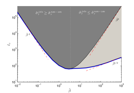
Figure 1: The critical energy input rate $\tilde{\varepsilon}_{c}$ for structural instability (thick solid line) and the critical energy input rate for structural instability of zonal jets (solid line) as a function of $\tilde{\beta}$. The behavior of these critical values for $\tilde{\beta}\ll 1$ and $\tilde{\beta}\gg 1$ is indicated with the dashed asymptotes. In the light gray region only non-zonal coherent structures emerge, while in the dark gray region both zonal jets and non-zonal coherent structures emerge. The thin dotted vertical line $\tilde{\beta}=\tilde{\beta}_{min}$ separates the unstable region: for $\tilde{\beta}<\tilde{\beta}_{min}$ zonal structures grow the most, whereas for $\tilde{\beta}>\tilde{\beta}_{min}$ non-zonal structures grow the most.

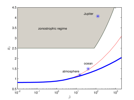
Figure 2: The critical zonostrophy parameter $R_{\beta}=0.7(\tilde{\varepsilon}_{c}\tilde{\beta}^{2})^{1/20}$ for structural instability (thick line) and the corresponding critical parameter for structural instability of zonal jets (thin line) as a function of $\tilde{\beta}$. The shaded region denotes the zonostrophic regime for which both the inequalities $R_{\beta}\geq 2.5$ and $k_{\beta}/K_{f}\leq 1/4$ are satisfied. The stars denote the position of the Earth’s atmosphere and ocean as well as the Jovian atmosphere in the $R_{\beta}$, $\tilde{\beta}$ parameter space.

We now examine the growth rate and dispersion properties of the unstable modes for $\tilde{\varepsilon}>\tilde{\varepsilon}_{c}$ and consider first the case $\tilde{\beta}=1$, with $\tilde{\varepsilon}=2\tilde{\varepsilon}_{c}$. The growth rate of the maximally growing eigenvalue, $\tilde{\sigma}_{r}$, and its associated frequency of the mode, $\tilde{\sigma}_{i}$, are plotted in figure 3(a) as a function of $|\tilde{n}|$ and $|\tilde{m}|$. We observe that the region in wavenumber space defined roughly by $0<|\tilde{n}|<1/2,\mbox{~{}and~{}}1/2<|\tilde{m}|<1$ is unstable, with the maximum growth rate occurring for zonal structures ($\tilde{n}=0$) with $|\tilde{m}|\simeq 0.8$. The frequency of the unstable modes is zero for zonal jet perturbations ($\tilde{n}=0$) and non-negative for all other wavenumbers ($\tilde{n}\neq 0$). Using the symmetries (17), this implies that real unstable mean flow perturbations $\delta Z$ propagate in the retrograde direction if $\tilde{n}\neq 0$ and are stationary when $\tilde{n}=0$. As $\tilde{\varepsilon}$ increases the instability region expands and roughly covers the sector $1/2<|\tilde{N}|<1$, with zonal structures having a larger growth rate compared to non-zonal structures, a result that holds for any $\tilde{\varepsilon}$ when $\tilde{\beta}<\tilde{\beta}_{min}$.

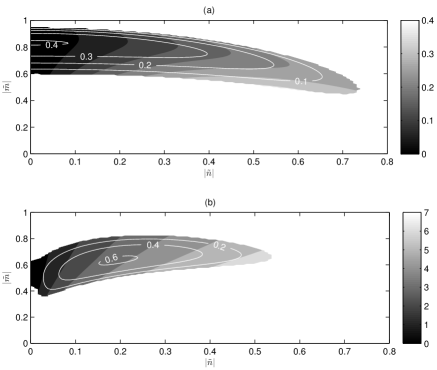
Figure 3: Dispersion relation of the unstable modes for $\tilde{\beta}=1$ (panel a) and $\tilde{\beta}=10$ (panel b). The contours show the growth rate $\tilde{\sigma}_{r}$ and the shading shows the frequency $\tilde{\sigma}_{i}$ of the unstable modes. For $\tilde{\beta}~{}O(1)$, stationary zonal jets are more unstable and for $\tilde{\beta}\gg 1$, westward propagating non-zonal structures are more unstable. For both panels, the energy input rate is $\tilde{\varepsilon}=2\tilde{\varepsilon}_{c}$.

For $\tilde{\beta}>\tilde{\beta}_{min}$ the non-zonal structures have always larger growth rate. This is illustrated in figure 3(b), showing the growth rates and frequencies of the unstable modes for $\tilde{\beta}=10$. For larger $\tilde{\beta}$ values there is a tendency for the frequency of the unstable modes to conform to the corresponding Rossby wave frequency

$$\tilde{\sigma}_{R}=\frac{\tilde{\beta}\tilde{n}}{\tilde{n}^{2}+\tilde{m}^{2}}~{},$$ (19)

a tendency that does not occur for smaller $\tilde{\beta}$. A comparison between the frequency of the unstable modes and the Rossby wave frequency is shown in figure 4 in a plot of $\tilde{\sigma}_{i}/\tilde{\sigma}_{R}$. For slightly supercritical $\tilde{\varepsilon}$, the ratio is close to one and the unstable modes satisfy the Rossby wave dispersion relation. At higher supercriticalities though, $\tilde{\sigma}_{i}$ departs from the Rossby wave frequency (by as much as $40\%$ for the case of $\tilde{\varepsilon}=50\tilde{\varepsilon}_{c}$ shown in figure 4(b)).

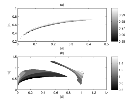
Figure 4: Ratio of the frequency of the unstable modes $\tilde{\sigma}_{i}$ over the corresponding frequency of a Rossby wave with the same wavenumbers $\tilde{\sigma}_{R}$ at (a) $\tilde{\varepsilon}=2\tilde{\varepsilon}_{c}$ and (b) $\tilde{\varepsilon}=50\tilde{\varepsilon}_{c}$ when $\tilde{\beta}=100$. Values of one denote an exact match with the Rossby wave frequency.

3 Analysis of the eddy-mean flow dynamics underlying jet formation

In this section, we investigate the eddy-mean flow dynamics leading to jet formation. These dynamics should have the property of directly channeling energy from the turbulent motions to the coherent flow without the presence of a turbulent cascade. Previous studies have identified such mechanisms for the maintenance of zonal jets. Huang and Robinson (1998) showed that shear straining of the turbulent field by the jet produced upgradient momentum fluxes that maintained the jet against dissipation. A simple case that clearly illustrates the physical picture for the mechanism of shear straining is to consider the evolution of eddies in a planar, inviscid constant shear flow. The eddies are sheared by the mean flow into thinner elliptical shapes, while their vorticity is conserved. For an elongated eddy this implies that the eddy velocities decrease and the eddy energy is transferred to the mean flow through upgradient momentum fluxes. This mechanism can operate when the time required for the eddies to shear over is much shorter than the dissipation time scale. The reason is that in this limit even the eddies with streamfunctions leaning against the shear that initially widen significantly gaining momentum, have the necessary time to shear over, elongate and surrender their momentum to the mean flow. Given that for an emerging jet the characteristic shear time scale is necessarily infinitely longer than the dissipation time scale, it needs to be shown that shear straining can produce upgradient momentum fluxes in this case as well. In addition, previous studies have shown that shearing of isotropic eddies on an infinite domain does not produce any net momentum fluxes (Shepherd 1985; Farrell 1987; Holloway 2010) and should have no effect on the S3T instability (Srinivasan and Young 2012). Therefore another mechanism should be responsible for producing the upgradient fluxes in the case of an isotropic forcing.

In order to investigate the eddy-mean flow dynamics underlying the S3T instability, we calculate the vorticity flux divergence that is induced when the statistical equilibrium (13) is perturbed by an infinitesimal coherent structure $\delta Z$. For an S3T unstable structure, the induced flux divergence tends to enhance the coherent structure $\delta Z$ producing the positive feedback required for instability. So the goal of this section is to illuminate the eddy-mean flow dynamics leading to this positive feedback and to understand qualitatively why the homogeneous equilibrium is more stable for small and large values of $\tilde{\beta}$.

For zonal mean flows (9), (12) are simplified to:

$$\partial_{t}U=-\partial_{y}\left<u^{\prime}v^{\prime}\right>-rU=\partial_{y}\left(\partial_{y_{2}x_{1}}^{2}\Delta_{1}^{-1}C\right)_{{\bf x}_{1}={\bf x}_{2}}-rU,$$ (20)

and

$$\partial_{t}C=(A_{1}+A_{2})C+\Xi,$$ (21)

where

$$A_{i}=-U_{i}\partial_{x_{i}}-(\beta-\partial_{y_{i}y_{i}}^{2}U)\Delta_{i}^{-1}\partial_{x_{i}}-r,$$ (22)

respectively. As a result the zonal mean flow is driven by the momentum flux divergence of the eddies. The perturbation in vorticity covariance $\delta C$ that is induced by the mean flow perturbation $\delta U$ can be estimated immediately by assuming that the system (20)-(21) is very close to the stability boundary, so that the growth rate is small. In this case the mean flow evolves slow enough that it remains in equilibrium with the eddy covariance, that is $d\delta C/dt\simeq 0$. Bakas and Ioannou (2013b) showed that the ensemble mean momentum flux induced by an infinitesimal sinusoidal mean flow perturbation $\delta U=\epsilon\sin(my)$, where $\epsilon\ll 1$ (i.e the eigenfunction of (B4)), is equal in this case to the integral over time and over all zonal wavenumbers of the responses to all point excitations in the $y$ direction:

$$\delta\left<u^{\prime}v^{\prime}\right>=\frac{1}{2\pi}\int_{-\infty}^{\infty}\int_{-\infty}^{\infty}\int_{0}^{\infty}\overline{u^{\prime}v^{\prime}}(t)dtd\xi dk,$$ (23)

where $\overline{u^{\prime}v^{\prime}}(t)$ is the momentum flux at time $t$ produced by:

$$G(k,y-\xi)=B(k)h(y-\xi)e^{ikx+il_{0}(y-\xi)}.$$ (24)

The Green’s function $G$ has the form of a wavepacket with an amplitude $B(k)$ and a carrier wave with wavenumbers $(k,l_{0})$ that is modulated in the $y$ direction by the wavepacket envelope $h(y)$. The characteristics of the amplitude, the wavenumber and the envelope depend on the forcing characteristics, but in any case the calculation of the ensemble mean momentum fluxes is reduced to calculating the momentum fluxes over the life cycle of wavepackets that are initially at different latitudes and then adding their relative contributions.

As the wavepacket propagates in the latitudinal direction, its meridional wavenumber and frequency are going to change due to shearing by the mean flow and due to the change of the mean vorticity gradient $\beta-U_{yy}$. The resulting time variable momentum flux $\overline{u^{\prime}v^{\prime}}(t)$ can be calculated using ray tracing. According to standard ray tracing arguments, the wave action is conserved along a ray (in the absence of dissipation) leading to the momentum flux:

$$\overline{u^{\prime}v^{\prime}}(t)=-|B|^{2}A_{M}(t)e^{-2rt}|h(y-\eta(t))|^{2},$$ (25)

where $A_{M}(t)=kl_{t}/(k^{2}+l_{t}^{2})^{2}$ is the momentum flux of the carrier wave that determines the amplitude of the fluxes of the wavepacket and $l_{t}$, $\eta(t)$ are the time dependent meridional wavenumber and position of the wavepacket respectively (Andrews et al. 1987). Because of the small amplitude of the mean flow perturbation $\delta U$, the wavenumber and position of the packet vary slowly on a time scale $O(\epsilon t)$ compared to the dissipation time scale $1/r$ and the dominant contribution to the time integral in (23) comes from small times. We can therefore seek asymptotic solutions of the form

$$l_{t}=l_{0}+\epsilon l_{1}+\cdots~{},~{}~{}~{}~{}\eta(t)=\xi+c_{0}t+\epsilon\eta_{1}(t)+\cdots~{},$$ (26)

where $c_{0}=2\beta kl_{0}/(k^{2}+l_{0}^{2})^{2}$ is the group velocity in the absence of a mean flow and calculate the integral of $\overline{u^{\prime}v^{\prime}}(t)$ over time from the leading order terms. Substituting (26) in (25) we obtain:

$$\overline{u^{\prime}v^{\prime}}(t) =\underbrace{-|B|^{2}A_{M}(0)e^{-2rt}|h(y-\xi-c_{0}t)|^{2}}_{\overline{u^{\prime}v^{\prime}}_{R}}-$$

$$\quad\underbrace{-\epsilon|B|^{2}\left(\frac{dA_{M}}{dl_{t}}\right)_{l_{0}}l_{1}(t)e^{-2rt}|h(y-\xi-c_{0}t)|^{2}}_{\overline{u^{\prime}v^{\prime}}_{S}}$$

$$\quad-\underbrace{\epsilon|B|^{2}A_{M}(0)\eta_{1}(t)e^{-2rt}\frac{d}{dy}|h(y-\xi-c_{0}t)|^{2}}_{\overline{u^{\prime}v^{\prime}}_{\beta}}.$$ (27)

The first term, $\overline{u^{\prime}v^{\prime}}_{R}$, arises from the momentum flux produced by a wavepacket in the absence of a mean flow. Because $A_{M}(0)=kl_{0}/(k^{2}+l_{0}^{2})^{2}$ is odd with respect to wavenumbers, this term does not contribute to the ensemble averaged momentum flux when integrated over all wavenumbers and will be hereafter ignored. The second term, $\overline{u^{\prime}v^{\prime}}_{S}$, arises from the small change in the amplitude of the flux $A_{M}$ over a dissipation time scale. The third term, $\overline{u^{\prime}v^{\prime}}_{\beta}$, arises from the small change in the position of the packet $\eta$ compared to a propagating packet in the absence of a mean flow. To summarize, the infinitesimal mean flow refracts the wavepacket due to shearing by the mean flow and due to the change of the mean vorticity gradient and slightly changes the amplitude of the fluxes as well as slightly speeds up or slows down the wavepacket. The sum of these two effects will produce the induced momentum fluxes.

a The limit of small scale wavepackets with a short propagation range

In order to clearly illustrate the behavior of the eddy fluxes, we consider the limit of $\tilde{\beta}=\beta L_{f}/r\ll 1$, where $L_{f}$ is the scale of the wavepackets and in addition we assume that the scale of the mean flow, $1/m$, is much larger than the scale of the wavepackets $mL_{f}\ll 1$. In this limit, the wavepackets are dissipated before propagating far from the initial position and the effect of the change in the mean vorticity gradient is higher order. As a result, Bakas and Ioannou (2013b) show that $l_{1}$ and $\eta_{1}$ decrease monotonically with time with rates independent of $\delta U_{yy}$ and proportional to the shear $\delta U_{y}(\xi)$ at the initial position $\xi$:

$$l_{1}=-\delta U_{y}(\xi)kt~{}~{},~{}~{}~{}~{}\eta_{1}=-\beta\delta U_{y}(\xi)\left(\frac{dA_{M}}{dl_{t}}\right)_{l_{0}}kt^{2}.$$ (28)

That is, the amplitude of the flux $A_{M}$ and the group velocity of the packets change only due to the shearing of the phase lines of the carrier wave according to the local shear.

Consider in this limit the first term, $\overline{u^{\prime}v^{\prime}}_{S}$, arising from the small amplitude change. Since the wavepacket is dissipated before it propagates away, we can ignore to first order propagation:

$$\overline{u^{\prime}v^{\prime}}_{S}= -\epsilon|B|^{2}\left(\frac{dA_{M}}{dl_{t}}\right)_{l_{0}}l_{1}(t)e^{-2rt}|h(y-\xi-c_{0}t)|^{2}$$

$$\simeq |B|^{2}\delta U_{y}(\xi)kt\left(\frac{dA_{M}}{dl_{t}}\right)_{l_{0}}e^{-2rt}|h(y-\xi)|^{2},$$ (29)

so that the packet grows/decays in situ. Since the wave packet is rapidly dissipated, the integrated momentum flux over its life time will be given to a good approximation by the instantaneous change in the flux that is proportional to $(dA_{M}/dl_{t})_{l_{0}}$. Figure 5 illustrates the amplitude of the momentum flux as a function of the angle $\theta_{t}=\arctan(l_{t}/k)$ of the phase lines of the carrier wave of the packet with the $y$-axis. It is shown that the momentum flux of a wavepacket with $|\theta_{0}|<\pi/6$ (that is with phase lines close to the meridional direction) excited in regions II or III, will increase within the dissipation time scale. Compared to an unsheared wavepacket, this process leads to upgradient momentum flux. The opposite occurs for waves excited in regions I and IV (with $|\theta_{0}|>\pi/6$) that produce downgradient flux, as their momentum flux decreases.

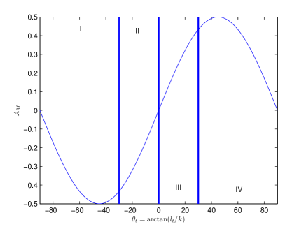
Figure 5: Amplitude of the momentum fluxes, $A_{M}(t)$, of wavepackets as a function of the angle $\theta_{t}=\arctan(l_{t}/k)$ between the phase lines of the central wave and the $y$-axis. The vertical lines separate the regions with $|\theta_{t}|<\pi/6$ (II and III) and $|\theta_{t}|>\pi/6$ (I and IV).

We now consider the second term, $\overline{u^{\prime}v^{\prime}}_{\beta}$ arising from the effect of propagation on the momentum flux. The group velocity is given by $c_{g}=2\beta A_{M}$ in this case and as a result a wavepacket starting in region III, will propagate towards the north (c.f. figure 5). Because shearing slows down the waves in region III ($\eta_{1}\sim-(dA_{M}/dl_{t})$), the wavepacket will flux its momentum from southern latitudes compared to when it moved in the absence of the shear flow. This is shown in figure 6(a) illustrating the distribution of momentum flux of an unsheared and a sheared perturbation whose amplitudes are constant. Figure 6(b) plots this difference, $\overline{u^{\prime}v^{\prime}}_{\beta}$, and shows that the flux is downgradient in this case. The same happens for waves excited in region II, while the waves excited in regions I and IV produce upgradient flux.

The net momentum fluxes produced by an ensemble of wavepackets, will therefore depend on the spectral characteristics of the forcing that determine the regions (I-IV), in which the forcing has significant power. Bakas and Ioannou (2013b) show that for the isotropic forcing (18):

$$\delta\left<u^{\prime}v^{\prime}\right>=$$

$$~{}~{}={1\over 2\pi}\int_{-\infty}^{\infty}\int_{-\infty}^{\infty}\overline{u^{\prime}v^{\prime}}_{S}d\xi dk+{1\over 2\pi}\int_{-\infty}^{\infty}\int_{-\infty}^{\infty}\overline{u^{\prime}v^{\prime}}_{\beta}d\xi dk$$

$$~{}~{}\simeq 0-{3\tilde{\varepsilon}\tilde{\beta}^{2}r\over 32\pi K_{f}^{4}}{d^{3}\delta U\over dy^{3}}.$$ (30)

The first integral is zero, because the gain in momentum occurring for $|\theta_{0}|<\pi/6$ (waves excited in regions II, III) is fully compensated by the loss in momentum for $|\theta_{0}|>\pi/6$ (waves excited in regions I, IV) since for the isotropic forcing all possible wave orientations are equally excited. The net momentum fluxes are therefore produced by the $\overline{u^{\prime}v^{\prime}}_{\beta}$ term and are upgradient, because the loss in momentum occurring for $|\theta_{0}|<\pi/6$, is over compensated by the gain in momentum for $|\theta_{0}|>\pi/6$. The momentum fluxes are also proportional to the third derivative of $\delta U$ yielding a hyper-diffusive momentum flux divergence that tends to reenforce the mean flow and is therefore destabilizing. These destabilizing fluxes are proportional to $\tilde{\beta}^{2}$ and as a result, the energy input rate required to form zonal jets increases as $1/\tilde{\beta}^{2}$ in this limit. It is worth noting that the first term integrates to zero only for the special case of the isotropic forcing, as even the slightest anisotropy yields a non-zero contribution from $\overline{u^{\prime}v^{\prime}}_{S}$. For example consider the forcing covariance $\Xi(x_{1},x_{2},y_{1},y_{2})=\cos\left(k(x_{1}-x_{2})\right)e^{-(y_{1}-y_{2})^{2}/\delta^{2}}$ that mimics the forcing of the barotropic flow by the most unstable baroclinic wave, which has zero meridional wavenumber. In this case the forcing that is centered at $l_{0}=0$ in wavenumber space, injects significant power in a band of waves in regions II and III and therefore $\overline{u^{\prime}v^{\prime}}_{S}$ yields upgradient fluxes.

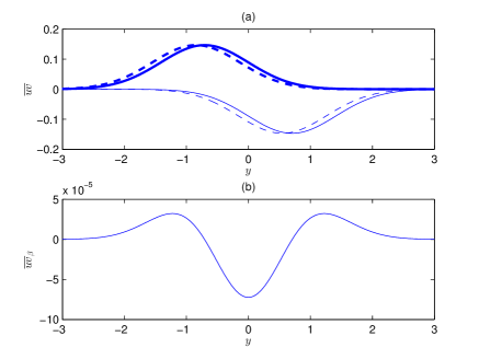
Figure 6: (a) Comparison of the momentum fluxes of an unsheared wavepacket excited in regions II (thick solid line) and III (solid line) to the momentum fluxes of a sheared wavepacket shown by the corresponding dashed lines, when only the change in propagation is taken into account. A snapshot of the fluxes at $t=0.2/r$ is shown. The planetary vorticity gradient is $\beta=0.1$, the wavepacket has initial vorticity $h(y)=e^{-y^{2}}$, $\sqrt{k^{2}+l_{0}^{2}}=1$, $|\theta_{0}|=\pi/10$ and $|B|=1$. (b) The difference in momentum fluxes between a sheared and an unsheared wavepacket calculated over their life cycle.

b The effects of the change in the mean vorticity gradient and the finite propagation range

In order to take into account the effect of the change in the vorticity gradient, we retain higher order terms with respect to $mL_{f}\ll 1$ in $l_{1}$ and $\eta_{1}$. In this case it can be shown that $l_{1}$ decreases with time at a rate proportional to $U_{y}(\xi)+U_{yyy}(\xi)$ (Bakas and Ioannou 2013b). Since the local shear and the local change in the vorticity gradient have different signs, the wavepacket is ’sheared less’ and as a result we expect reduced momentum fluxes compared to the limit discussed in section 4.2. Indeed, for the isotropic forcing:

$$\delta\left<u^{\prime}v^{\prime}\right>\simeq-{3\tilde{\varepsilon}\tilde{\beta}^{2}r\over 32\pi K_{f}^{4}}\left({d^{3}\delta U\over dy^{3}}-\frac{1}{4K_{f}^{2}}\frac{d^{5}\delta U}{dy^{5}}\right).$$ (31)

That is, the change in the mean vorticity gradient has a stabilizing effect.

We finally relax the assumption that $\tilde{\beta}\ll 1$. In this case, $l_{1}$ and $\eta_{1}$ are affected by an integral shear and mean vorticity gradient over the region of propagation. For larger $\tilde{\beta}$, the wavepacket will encounter regions of both positive and negative shear and as a result, the momentum fluxes that are qualitatively proportional to the integral shear over the propagation region will be reduced. In the limit $\tilde{\beta}\gg 1$, the region of propagation is the whole sinusoidal flow with consecutive regions of positive and negative shear and the integral shear along with the fluxes will asymptotically tend to zero. As a result, the energy input rate required for structural instability of zonal jets increases with $\tilde{\beta}$ in this limit.

4 Equilibration of the S3T instabilities

We now investigate the equilibration of the instabilities by studying the S3T system (9), (12) discretized in a doubly periodic channel of size $2\pi\times 2\pi$. We approximate the monochromatic forcing (18), by considering the narrow band forcing

$$\hat{\Xi}(k,l)=\frac{K_{f}}{\Delta K_{f}}\left\{\begin{array}[]{ll}1,~{}\mbox{for~{}}|\sqrt{k^{2}+l^{2}}-K_{f}|\leq\Delta K_{f}\\ 0,~{}\mbox{for~{}}|\sqrt{k^{2}+l^{2}}-K_{f}|>\Delta K_{f}\end{array}\right.,$$ (32)

where $k$, $l$ assume integer values, that injects energy at rate $\varepsilon$ in a narrow ring in wavenumber space with radius $K_{f}$ and width $\Delta K_{f}$. We consider the set of parameter values $\beta=10$, $r=0.01$, $\nu=1.19\cdot 10^{-6}$, $K_{f}=10$ and $\Delta K_{f}=1$, for which $\tilde{\beta}=100$. The integration is therefore in the parameter region of figure 1 in which the non-zonal structures are more unstable than the zonal jets. The growth rates of the coherent structures for integer values of the wavenumbers, $n$ and $m$ are calculated from the discrete version of equation (15) obtained by substituting the integrals with sums over integer values of the wavenumbers (Bakas and Ioannou 2013a).

We first consider the supercritical energy input rate $\tilde{\varepsilon}=4\tilde{\varepsilon}_{c}$. For these parameters only non-zonal modes are unstable, with the perturbation with $(n,m)=(1,5)$ growing the most. At $t=0$, we introduce a small random perturbation, whose streamfunction is shown in figure 7(a). After a few e-folding times, a harmonic structure of the form $Z=\cos(x)\cos(5y)$ dominates the large-scale flow. The energy of this large scale structure shown in figure 7(b), increases rapidly and eventually saturates. At this point the large-scale flow gets attracted to a traveling wave finite amplitude equilibrium structure (cf. figure 7(c)) close in form to the harmonic $Z=\cos(x)\cos(5y)$ that propagates westward. This is illustrated in the Hovmöller diagram of $\psi(x,y=\pi/4,t)$ shown in 7(d). The sloping dashed line in the diagram corresponds to the phase speed of the traveling wave, which is found to be approximately the phase speed of the unstable $(n,m)=(1,5)$ eigenmode.

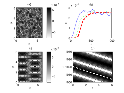
Figure 7: Equilibration of the S3T instabilities. (a) Streamfunction of the initial perturbation. (b) Energy evolution of the initial perturbation shown in panel (a) as obtained from the integration of the S3T equations (9) and (12) (dashed line) and from the integration of the ensemble quasi-linear (EQL) system (4)-(3) with $N_{\textrm{ens}}=10$ (solid line) and $N_{\textrm{ens}}=100$ (dash-dotted line) ensemble members that is discussed in section 6. (c) Snapshot of the streamfunction $\Psi_{eq}$ of the traveling wave structure and (d) Hovmöller diagram of $\Psi_{eq}(x,y=\pi/4,t)$ for the finite equilibrated traveling wave. The thick dashed line shows the phase speed obtained from the stability equation (15). The energy input rate is $\tilde{\varepsilon}=4\tilde{\varepsilon}_{c}$ and $\tilde{\beta}=100$.

Consider now the energy input rate $\tilde{\varepsilon}=10\tilde{\varepsilon}_{c}$. While the maximum growth rate still occurs for the $(|n|,|m|)=(1,5)$ non-zonal structure, zonal jet perturbations are unstable as well. If the S3T dynamics are restricted to account only for the interaction between zonal flows and turbulence by employing a zonal mean rather than an ensemble mean, an infinitesimal jet perturbation will grow and equilibrate at finite amplitude. To illustrate this we integrate the S3T dynamical system (20)-(21) restricted to zonal flow coherent structures. The energy of the small zonal jet perturbation $\delta Z=0.1\cos(4y)$ is shown in figure 8 to grow and saturate at a constant value and the streamfunction of the equilibrated jet is shown in the left inset in figure 8. However, in the context of the generalized S3T analysis that takes into account the dynamics of the interaction between coherent non-zonal structures and jets, we find that these S3T jet equilibria can be saddles: stable to zonal jet perturbations but unstable to non-zonal perturbations. To show this, we consider the evolution of the same jet perturbation $\delta Z=0.1\cos(4y)$ under the generalized S3T dynamics (9), (12) and find that the flow follows the zonally restricted S3T dynamics and equilibrates to the same finite amplitude zonal jet (cf. figure 8). At this point we insert a small random perturbation to the equilibrated flow. Soon after, non-zonal undulations grow and the flow transitions to the stable $Z=\cos(x)\cos(5y)$ traveling wave state that is also shown in figure 8. As a result, the finite equilibrium zonal jet structure is S3T unstable to coherent non-zonal perturbations and is not expected to appear in non-linear simulations despite the fact that the zero flow equilibrium is unstable to zonal jet perturbations. We will elaborate more on this issue in the next section.

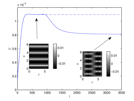
Figure 8: Energy evolution of an initial jet perturbation $\delta Z=0.1\cos(4y)$ for the zonally restricted S3T dynamics (20)-(21) (dashed line) and the generalized S3T dynamics (9), (12) (thin line). The insets show a snapshot of the mean flow streamfunction at $t=700$ (left) and the streamfunction of the equilibrated structure at $t=3500$ (right) under the generalized S3T dynamics. The parameters are $\tilde{\varepsilon}=10\tilde{\varepsilon}_{c}$ and $\tilde{\beta}=100$.

Finally, consider the case $\tilde{\varepsilon}=30\tilde{\varepsilon}_{c}$. At this energy input rate, the finite amplitude non-zonal traveling wave equilibria become S3T unstable. To show this, we consider the non-zonal traveling wave equilibrium obtained by the evolution of the small non-zonal perturbation $\delta Z=0.01\cos(x)\cos(5y)$ to the homogeneous state that is shown at the left inset in figure 9 and impose a small random zonal perturbation. The evolution of the zonal energy $E_{z}=(1/2)\overline{U}^{2}$, where the overbar denotes a zonal average, is shown in figure 9. After an initial transition period, the zonal perturbations grow exponentially and the flow transitions to the jet equilibrium state shown at the right inset in figure 9. Note however, that the jet equilibrium structure is not zonally symmetric. This is a new type of S3T equilibrium: it is a mix between a zonal jet and a non-zonal traveling wave with the same meridional scale. These mixed equilibria appear to be the attractors for larger energy input rates as well. This is illustrated in figure 10 showing the structure of the mixed equilibrium at $\varepsilon=50\varepsilon_{c}$. The equilibrium structure consists of a large amplitude zonally symmetric jet with larger scale compared to the mixed state in figure 9. Embedded in it are non-zonal vortices with the same meridional scale and with about $14\%$ the energy of the zonal jet. These vortices that are shown in figure 10(b) to have approximately the compact support structure $\Psi=\cos(x)\cos(4y)$ propagate westward as shown in the Hovmöller diagram in figure 10(c).

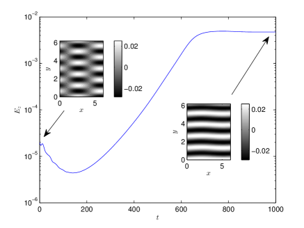
Figure 9: Zonal energy evolution of a random zonal perturbation imposed on the non-zonal traveling wave equilibrium shown in the left inset. The streamfunction of the equilibrated structure is shown in the right inset. The energy input rate is $\tilde{\varepsilon}=30\tilde{\varepsilon}_{c}$ and $\tilde{\beta}=100$.

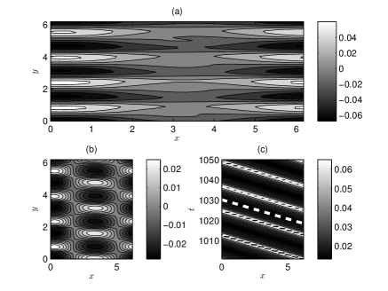
Figure 10: Mixed zonal jet-traveling wave S3T equilibrium for $\tilde{\varepsilon}=50\tilde{\varepsilon}_{c}$ and $\tilde{\beta}=100$. (a) Snapshot of the streamfunction $\Psi_{eq}$ of the equilibrium state. (b) Contour plot of the non-zonal component $\Psi_{eq}-\overline{\Psi_{eq}}$ of the equilibrium structure, where the overline denotes a zonal average. (c) Hovmöller diagram of $\Psi_{eq}(x,y=\pi/4,t)$ for the equilibrated structure.

5 Comparison to ensemble mean quasi-linear and non-linear simulations

a Comparison to an ensemble of quasi-linear simulations

Within the context of the second order cumulant closure, the S3T formulation allows the identification of statistical turbulent equilibria in the infinite ensemble limit, in which the fluctuations induced by the stochastic forcing are averaged to zero. However, these S3T equilibria and their stability properties are manifest even in single realizations of the turbulent system. For example, previous studies using S3T obtained zonal jet equilibria in barotropic, shallow water and baroclinic flows in close correspondence with observed jets in planetary flows (Farrell and Ioannou 2007, 2008, 2009b, 2009a). In addition, previous studies of S3T dynamics restricted to the interaction between zonal flows and turbulence in a $\beta$-plane channel showed that when the energy input rate is such that the zero mean flow equilibrium is unstable, zonal jets also appear in the non-linear simulations with the structure (scale and amplitude) predicted by S3T (Srinivasan and Young 2012; Constantinou et al. 2014).

A very useful intermediate model that retains the wave-mean flow dynamics of the S3T system while relaxing the infinite ensemble approximation is the quasi-linear system (5)-(6). Under the ergodic assumption, this can be interpreted as an ensemble of quasi-linear equations (EQL) in which the ensemble mean can be calculated from a finite number of ensemble members. Its integration is done as follows. A pseudo-spectral code with a $128\times 128$ resolution and a fourth order Runge-Kutta scheme for time stepping is used to integrate (5)-(6) forward. At each time step, $N_{\textrm{ens}}$ separate integrations of (6) are performed with the eddies evolving according to the instantaneous flow. Then the ensemble average vorticity flux divergence is calculated as the average over the $N_{\textrm{ens}}$ simulations and (5) is stepped forward in time according to those fluxes. The EQL system reaches a statistical equilibrium at time scales of the order of $t_{eq}\sim O(1/r)$ and the integration was carried on until $t=100t_{eq}$ in order to collect accurate statistics.

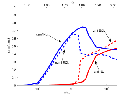
Figure 11: The zmf and nzmf indices defined in (33) and (35) respectively, as a function of energy input rate $\varepsilon/\varepsilon_{c}$ and the zonostrophy parameter $R_{\beta}$ for the non-linear (NL) integrations and an ensemble of quasi-linear (EQL) integrations (dashed line) with $N_{\textrm{ens}}=10$ ensemble members as described in section 6. The critical value $\varepsilon_{c}=8.4\cdot 10^{-6}$ is the energy input rate at which the S3T predicts structural instability of the homogeneous turbulent state. Zonal jets emerge for $\varepsilon>\varepsilon_{nl}$, with $\varepsilon_{nl}=15\varepsilon_{c}$. The parameters are $\beta=10$, $r=0.01$, $\nu=1.19\cdot 10^{-6}$ and the forcing is an isotropic ring in wavenumber space with radius $K_{f}=10$ and width $\Delta K_{f}=1$.

We choose the same parameter values as in the S3T integrations in section 5 ($\beta=10$, $r=0.01$, $\nu=1.19\cdot 10^{-6}$, $K_{f}=10$ and $\Delta K_{f}=1$). For these parameters ($\tilde{\beta}=100$), S3T predicts the emergence of propagating non-zonal structures when the energy input rate exceeds the critical threshold $\tilde{\varepsilon}_{c}$, and the emergence of mixed zonal jet-traveling wave states when the finite amplitude traveling wave states become structurally unstable to zonal jet perturbations. In order to examine whether the same bifurcations occur in the EQL system, we consider two indices that measure the power concentrated at scales larger than the scales forced. The first is the zonal mean flow index defined as in Srinivasan and Young (2012), as the ratio of the energy of zonal jets with scales larger than the scale of the forcing over the total energy

$$\mbox{zmf}=\frac{\sum_{l:l<K_{f}-\Delta K_{f}}\hat{E}(k=0,l)}{\sum_{kl}\hat{E}(k,l)},$$ (33)

where

$$\hat{E}(k,l)=\frac{1}{2T}\int_{0}^{T}\left(\left<\frac{|\hat{\zeta}^{\prime}|^{2}}{k^{2}+l^{2}}\right>+\frac{|\hat{Z}|^{2}}{k^{2}+l^{2}}\right)dt$$ (34)

is the time averaged total energy power spectrum of the flow at wavenumbers $(k,l)$. The second is the non-zonal mean flow index defined as the ratio of the energy of the non-zonal modes with scales larger than the scale of the forcing over the total energy:

$$\mbox{nzmf}=\frac{\sum_{kl:K<K_{f}-\Delta K_{f}}\hat{E}(k,l)}{\sum_{kl}\hat{E}(k,l)}-\mbox{zmf}.$$ (35)

If the structures that emerge are coherent, then these indices quantify their amplitude. Figure 11 shows both indices as a function of the energy input rate $\varepsilon$ and as a function of the corresponding values of the zonostrophy index $R_{\beta}$ for EQL simulations with $N_{\textrm{ens}}=10$ members. The rapid increase of the nzmf index for $\varepsilon>\varepsilon_{c}$ (corresponding to $R_{\beta}>1.55$), illustrates that this regime transition in the flow predicted by S3T with the emergence of non-zonal structures manifests in the quasi-linear dynamics as well. We now consider the case $\varepsilon=4\varepsilon_{c}$ in detail in which the traveling wave structure $Z=\cos(x)\cos(5y)$ is maintained in the S3T integrations. We observe, that the S3T equilibria manifest in the EQL simulations with the addition of some ’thermal noise’ due to the stochasticity of the forcing that is retained in this system. This is illustrated in figure 7b showing the energy growth of the coherent structure for $N_{\textrm{ens}}=10$ and $N_{\textrm{ens}}=100$. The energy of the coherent structure in the EQL integrations fluctuates around the values predicted by the S3T system with the fluctuations decreasing as $1/\sqrt{N_{\textrm{ens}}}$. However, even with only 10 ensemble members we get an estimate that is very close to the theoretical estimate of the infinite ensemble members obtained from the S3T integration. The structure of the traveling wave equilibrium in the quasi-linear simulations shown in figure 12(a) and its phase speed (not shown) are also in very good agreement with the corresponding structure and phase speed obtained from the S3T integration.

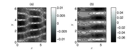
Figure 12: Snapshot of the mean streamfunction $\Psi$ at statistical equilibrium obtained from the ensemble mean quasi-linear simulations with $N_{\textrm{ens}}=10$ members for $\varepsilon=4\varepsilon_{c}$ (panel a) and $\varepsilon=50\varepsilon_{c}$ (panel b). The parameters are as in figure 11.

The second transition in which zonal jets emerge is more intriguing. While the homogeneous equilibrium is structurally unstable to zonal jets when $\varepsilon_{sz}=5.2\varepsilon_{c}$, the finite amplitude zonal jet equilibria are structurally unstable and the flow stays on the attractor of the non-zonal traveling wave equilibria (cf. figure 8). When $\varepsilon>\varepsilon_{nl}$, the non-zonal traveling wave equilibria become S3T unstable while at these parameter values the S3T system has mixed zonal jet-traveling wave equilibria which are stable (cf. figure 10). The rapid increase in the zmf index with the concomitant rapid decrease in the nzmf index shown in figure 11, illustrates that this regime transition manifests in the EQL system as well with similar mixed zonal-traveling wave states appearing. The structure of the mixed zonal jet-traveling wave equilibrium for $\varepsilon=50\varepsilon_{c}$ is shown in 12(b) and similar to the S3T equilibrium in figure 10, it consists mainly of 4 zonal jets and the compact support vortices $Z\sim\cos(x)\cos(4y)$ embedded in the jets. We therefore conclude that the EQL system accurately captures the characteristics of the emerging structures.

b Comparison to non-linear simulations

In order to compare the predictions of S3T to the non-linear simulations, we solve (1) with the narrow band forcing (32) on a doubly periodic channel of size $2\pi\times 2\pi$ using the same pseudospectral code as in the EQL simulations and the same parameter values. Figure 11 shows the nzmf and zmf indices as a function of the energy input rate $\varepsilon$ for the NL simulations. The rapid increase in the nzmf index for $\varepsilon>\varepsilon_{c}$ shows that the non-linear dynamics share the same bifurcation structure as the S3T statistical dynamics. In addition, the stable S3T equilibria are in principle viable repositories of energy in the turbulent flow and the non-linear system is expected to visit their attractors for finite time intervals. Indeed for $\varepsilon=4\varepsilon_{c}$, the pronounced peak at $(|k|,|l|)=(1,5)$ of the time averaged power spectrum shown in figure 13(a) illustrates that the traveling wave equilibrium with $(|k|,|l|)=(1,5)$ that emerges in the S3T integrations, is the dominant structure in the NL simulations. Comparison of the energy spectra obtained from the EQL and the NL simulations (not shown), reveals that the amplitude of this structure in the quasi-linear and in the non-linear dynamics almost matches. Remarkably, the phase speed of the S3T traveling wave matches with the corresponding phase speed of the $(|k|,|l|)=(1,5)$ structure observed in the NL simulations, as can be seen in the Hovmöller diagram in figure 13(b). Such an agreement in the characteristics of the emerging structures between the EQL and NL simulations occurs for a wide range of energy input rates as can be seen by comparing the nzmf indices in figure 11. As a result, S3T predicts the dominant non-zonal propagating structures in the non-linear simulations, as well as their amplitude and phase speed.

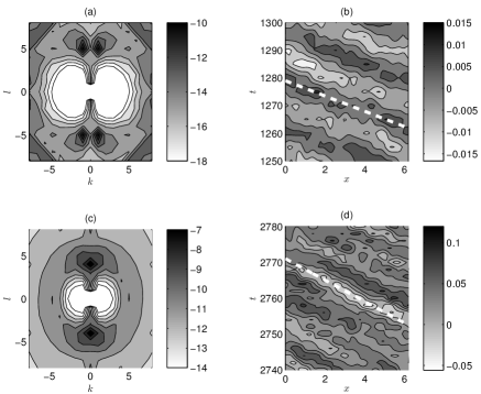
Figure 13: Time averaged energy power spectra, $\log(\hat{E}(k,l))$, obtained from the non-linear (NL) simulation of (1) at $\varepsilon/\varepsilon_{c}=4$ (panel a) and $\varepsilon/\varepsilon_{c}=50$ (panel c). Hovmöller diagram of $\psi(x,y=\pi/4,t)$ at $\varepsilon/\varepsilon_{c}=4$ (panel b) and $\varepsilon/\varepsilon_{c}=50$ (panel d). The thick dashed lines correspond to the phase speed obtained from the eigenvalue relation (15).

We now focus on the second regime transition with the emergence of zonal jets. The increase in the zmf index in the NL simulations for $\varepsilon>\varepsilon_{nl}$ that is shown in figure 11, indicates the emergence of jets roughly at the bifurcation point of the S3T and EQL simulations. However, the energy input rate threshold for the emergence of jets is larger in the NL simulations compared to the corresponding EQL threshold. This discrepancy possibly occurs due to the fact that the exchange of instabilities between the mixed jet-traveling wave equilibria and the pure traveling wave equilibria depends on the equilibrium structure $[Z^{E},C^{E}]$. Small changes for example in $C^{E}$ that might be caused by the eddy-eddy terms neglected in S3T can cause the exchange of instabilities to occur at slightly different energy input rates. It was shown in a recent study that when the effect of the eddy-eddy terms is taken into account by obtaining $C^{E}$ directly from the nonlinear simulations, the S3T stability analysis performed on this corrected equilibrium states accurately predicts the energy input rate for the emergence of jets in the nonlinear simulations (Constantinou et al. 2014). The power spectrum obtained from the NL simulations for $\varepsilon=50\varepsilon_{c}$ shows an energy peak at $(k,|l|)=(0,4)$ with secondary power peaks at $(|k|,|l|)=(1,4)$ and $(|k|,|l|)=(1,5)$) (of approximately $12\%$ of the energy in the zonal jet each). The Hovmöller diagram of the streamfunction shown in figure 13(d) reveals that the dominant non-zonal structures in the NL simulations propagate in the retrograde direction. As a result the mixed S3T equilibrium of figure 10 manifests in the NL simulations. Note however, that the phase speed calculated from the diagram is different than the phase speed of the $(|k|,|l|)=(1,4)$ structure in figure 10. At larger energy input rates the zonal jets have typically larger scales due to jet merging and coexist with energetically significant westward propagating non-zonal structures having an energy between $10-50\%$ of the jet energy and scales $(|k|,|l|)=(1,m)$, where $m$ is the number of jets in the channel. Such an agreement again holds for a wide range of energy input rates, as the zmf indices obtained from the EQL and the NL simulations indicate. In summary, S3T predicts the characteristics of both non-zonal propagating structures and of zonal jets in the non-linear simulations.

c Zonostrophic regime

S3T and the corresponding ensemble quasi-linear system were obtained by ignoring the eddy-eddy non-linear interactions. Therefore the question arises on whether the predictions of S3T are useful in the zonostrophic regime. In this regime, which is highly supercritical with respect to S3T instability of the homogeneous equilibrium (cf. figure 2), maintenance of zonal jets and zonons were interpreted by previous studies to arise from an inverse energy cascade (Galperin et al. 2010), a highly non-linear process, which is absent in S3T. According to this interpretation, the turbulent energy cascades isotropically toward large scales until it reaches $k_{\beta}$. At this scale the cascade becomes anisotropic and most of the energy is channelled into the zonal flows. To illustrate this, the time averaged energy power spectra $\hat{E}(k,l)$ are typically split between the zonal spectra $\hat{E}_{z}(l)=\hat{E}(k=0,l)$ and the residual $\hat{E}_{R}(k,l)=\hat{E}-\hat{E}_{z}$. The zonal and residual spectra calculated from NL integrations in the zonostrophic regime ($K_{f}=60$, $\Delta K=1$, $\beta=42$, $r=0.01$, $\varepsilon=0.0065$) are shown in figure 14. Up to the scale $k_{\beta}$, the residual spectra follow the Kolmogorov $K^{-5/3}$ law in accordance with an isotropic cascade assumption. At this scale, the cascade is anisotropized and the residual spectra steepen. However, most of the energy is in zonal scales with the zonal spectra following a much steeper $K^{-5}$ law.

The residual and the zonal spectra obtained from an EQL simulation with $N_{\textrm{ens}}=10$ for the same parameters, are also shown in figure 14. The residual spectra follow a shallower than $K^{-5/3}$ slope for $K>k_{\beta}$, while they steepen after $k_{\beta}$ and reach a lower peak with respect to the corresponding spectra from the NL simulations. In addition, the residual part of the spectrum corresponds mainly to incoherent motions for scales with $K>k_{\beta}$. This is revealed by taking into account only the spectra of the coherent part of the flow and calculating the residual spectrum that is also shown in figure 14. For most of the scales, it is at least one to two orders of magnitude lower than the corresponding residual spectrum when both coherent and incoherent motions are taken into account and only the non-zonal structures with large scales (close to the energy peak) appear to be coherent. Failure of the EQL simulations to exactly reproduce the $K^{-5/3}$ slope of the incoherent turbulent motions is not surprising, since the inverse energy cascade that is absent in the EQL simulations is essential for this part of the spectrum. The energetically important part however, which contains the large-scale energetic waves is captured by S3T. The zonal spectra obtained from the EQL simulations follow the same $K^{-5}$ law and peak at the same scale compared to the NL simulations but the peak has a larger amplitude. As is argued in section 5.2.2, the steep power law is an artifact of the shape of the strongly forced jet which is characterized by near discontinuity in the shear at the maxima of the prograde jets.

So to summarize, the scale and the shape of the dominant jet structure, as well as the scale of the most energetic coherent non-zonal structures are accurately captured by the EQL simulations, while the eddy-eddy interactions neglected in the EQL simulations set the proper scaling for the tail of the spectrum that consists of incoherent turbulent motions and change the partition between the energy of the jet (that is overestimated in the EQL simulations) and that of the non-zonal large-scale structures (that is underestimated in the EQL simulations).

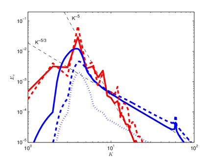
Figure 14: Residual (blue) and zonal (red) energy spectra for the NL (solid) and EQL (dashed) simulations in the zonostrophic regime. Also shown are the residual spectra from the EQL simulations when only the coherent motions are taken into account (blue dotted line). The parameters are $K_{f}=60$, $\Delta K=1$, $\beta=42$, $r=0.01$, $\varepsilon=0.0065$, for which $\tilde{\beta}=70$, $\tilde{\varepsilon}=7308\tilde{\varepsilon}_{c}$, $k_{\beta}=12.9$ and $R_{\beta}=2.5$. Lines (thin dashed) of slope $K^{-5/3}$ and $K^{-5}$ are also plotted for reference. The pseudo-spectral code was run with a $512\times 512$ resolution and the exponential filter of Smith et al. (2002) instead of hyper-diffusion.

6 Summary – Discussion

This article addressed the emergence of coherent structures in barotropic $\beta$-plane turbulence using the tools of Stochastic Structural Stability Theory (S3T), a statistical theory that expresses the statistics of the turbulent flow dynamics as a systematic cumulant expansion truncated at second order. With the interpretation of the ensemble average as a Reynolds average over the fast turbulent eddies adopted in this contribution, the second order cumulant expansion results in a closed, non-linear dynamical system that governs the joint evolution of slowly varying, spatially localized coherent structures with the second order statistics of the rapidly evolving turbulent eddies. The fixed points of this autonomous, deterministic non-linear system define statistical equilibria, the stability of which are amenable to the usual treatment of linear and non-linear stability analysis.

The linear stability of the homogeneous S3T equilibrium with no mean velocity was examined analytically for the case of an isotropic random stirring that sustains the turbulence in the barotropic flow. Structural instability was found to occur for perturbations with smaller scale than the forcing, when the energy input rate $\tilde{\varepsilon}=\varepsilon K_{f}^{2}/r^{3}$ is larger than a certain threshold $\tilde{\varepsilon}_{c}$ that depends on $\tilde{\beta}=\beta/(rK_{f})$. It was found that when $\tilde{\beta}$ is small or order one, the maximum growth rate occurs for stationary zonal structures, while for large $\tilde{\beta}$, westward propagating non-zonal grow the most.

The eddy–mean flow dynamics underlying the S3T instability of zonal jets was then studied in detail. It was shown that close to the structural stability boundary, the dynamics can be split into two competing processes. The first, which is shearing of the eddies by the local shear described by Orr dynamics in the $\beta$ plane, was shown to lead to jet forming upgradient momentum fluxes acting exactly as negative viscosity for an anisotropic forcing and as negative hyperviscosity for isotropic forcing. The second, which is momentum flux divergence resulting from lateral wave propagation on the nonuniform local mean vorticity gradient, was shown to lead to jet opposing downgradient fluxes acting as hyperdiffusion.

The equilibration of the unstable, exponentially growing coherent structures for large $\tilde{\beta}$ was then studied through numerical integrations of the S3T dynamical system. When the forcing amplitude is slightly supercritical, the finite amplitude traveling wave equilibrium has a structure close to the corresponding unstable non-zonal perturbation with the same scale. When the forcing amplitude is highly supercritical, the instabilities equilibrate to mixed states consisting of strong zonal jets with smaller amplitude traveling waves embedded in them.

The predictions of S3T were then compared to the results obtained from direct numerical simulations of the turbulent dynamics. The critical threshold above which coherent non-zonal structures are unstable according to the stability analysis of the S3T system was found to be in excellent agreement with the critical value above which non-zonal structures acquire significant power in the non-linear simulations. The scale, phase speed and amplitude of the dominant structures in the non-linear simulations were also found to correspond to the structures predicted by S3T. In addition, the threshold for the emergence of jets, which is identified in S3T as the energy input rate at which an S3T stable, finite amplitude zonal jet equilibrium exists, was found to roughly match the corresponding threshold for jet formation in the non-linear simulations, with the emerging jet scale and amplitude being accurately obtained using S3T. Such a good agreement between the predictions of S3T and direct numerical simulations, holds not only close to the bifurcation point for the emergence of coherent structures but also in the regime of zonostrophic turbulence. Consequently, these results provide a concrete example that large-scale structure in barotropic turbulence, whether it is zonal jets or non-zonal coherent structures, emerges and is sustained from systematic self-organization of the turbulent Reynolds stresses by spectrally non-local interactions and in the absence of a turbulent cascade.

APPENDIX A

Boundedness of the solutions and invariants of the S3T equations

The S3T system in the absence of forcing and dissipation has similar quadratic invariants with the nonlinear system. Further, the solutions of the S3T equations remain bounded for all times. That is, the sum of the enstrophy of the ensemble mean over the domain, $H_{m}=1/2\int{Z^{2}}dxdy$, and the eddy enstrophy over the domain, $H_{p}=1/2\int{C_{\mathbf{x}_{1}=\mathbf{x}_{2}}}dxdy$, is conserved. Similarly, the sum of the energy of the ensemble mean, $E_{m}=1/2\int{(U^{2}+V^{2})}dxdy$, and the eddy energy, $E_{p}=1/2\int(\Delta_{1}^{-1}{C)_{\mathbf{x}_{1}=\mathbf{x}_{2}}}dxdy$, is also conserved. We show this by first multiplying (9) (in the absence of hyper-diffusion) by $Z$ to obtain:

$$\partial_{t}\eta_{m}+U\partial_{x}\eta_{m}+V\partial_{y}\eta_{m}+\beta VZ=-Z\nabla\cdot\left<{\bf u}^{\prime}\zeta^{\prime}\right>-2r\eta_{m},$$ (A1)

where $\eta_{m}=Z^{2}/2$ is the enstrophy density of the ensemble mean. Integrating by parts and using the continuity equation we rewrite the advection terms as:

$$U\partial_{x}\eta_{m}+V\partial_{y}\eta_{m}=\partial_{x}(U\eta_{m})+\partial_{y}(V\eta_{m}).$$ (A2)

Writing $Z=\partial_{x}V-\partial_{y}U$ and using again the continuity equation we have:

$$ZV=\partial_{x}\frac{U^{2}+V^{2}}{2}-\partial_{y}(UV),$$ (A3)

and (A1) becomes:

$$\partial_{t}\eta_{m}+\nabla\cdot({\bf U}\eta_{m})+\beta\partial_{x}e_{m}-\beta\partial_{y}(UV)=-Z\nabla\cdot\left<{\bf u}^{\prime}\zeta^{\prime}\right>-2r\eta_{m},$$ (A4)

where $e_{m}=(1/2)(U^{2}+V^{2})$ is the energy density of the ensemble mean. Similarly it can be shown from (12), that the ensemble mean of the eddy enstrophy density $\eta_{p}=(1/2)C_{\mathbf{x}_{1}=\mathbf{x}_{2}}$ evolves (in the absence of hyper-diffusion) according to:

$$\partial_{t}\eta_{p}+\nabla\cdot({\bf U}\eta_{p})+\beta\left[\partial_{x}(e_{p})-\partial_{y}\left<u^{\prime}v^{\prime}\right>\right]+$$

$$\qquad+\left<u^{\prime}\zeta^{\prime}\right>\partial_{x}Z+\left<v^{\prime}\zeta^{\prime}\right>\partial_{y}Z=\eta_{f}-2r\eta_{p},$$ (A5)

where $e_{p}=(1/2)(\Delta_{1}^{-1}C)_{\mathbf{x}_{1}=\mathbf{x}_{2}}$ is the ensemble mean of the eddy energy density and $\eta_{f}=(1/2)\Xi_{\mathbf{x}_{1}=\mathbf{x}_{2}}$ is the enstrophy density of the forcing. Adding (A4) and (A5) we obtain the equation for the evolution of the total enstrophy density $\eta=\eta_{p}+\eta_{m}$:

$$(\partial_{t}+2r)\eta-\eta_{f}=-\nabla\cdot({\bf U}\eta)-\beta\partial_{x}(e_{p}+e_{m})+\beta\partial_{y}(UV+\left<u^{\prime}v^{\prime}\right>).$$ (A6)

Integrating (A6) over the horizontal domain, the terms on the rhs of (A6) integrate to zero and the total enstrophy $H=H_{m}+H_{p}=\int(\eta_{m}+\eta_{p})dxdy$ evolves according to:

$$\partial_{t}H=H_{f}-2rH,$$ (A7)

where $H_{f}$ is the total enstrophy imparted by the forcing. As a result, the enstrophy is bounded and has the value $H^{eq}=H_{f}/(2r)$ at steady state. Similarly, it can be shown that the total energy $E=E_{m}+E_{p}$ is bounded.

APPENDIX B

Calculation of the dispersion relation and its properties

In this Appendix we derive the dispersion relation (15), which determines the stability of zonal as well as non-zonal perturbations in homogeneous turbulence. We follow closely the treatment of Srinivasan and Young (2012). We first rewrite (9), (12) in terms of the variables $\tilde{x}=x_{1}-x_{2}$, $\overline{x}=(1/2)(x_{1}+x_{2})$, $\tilde{y}=y_{1}-y_{2}$ and $\overline{y}=(1/2)(y_{1}+y_{2})$. The derivatives transform into this new system of coordinates to $\partial_{x_{i}}=(1/2)\partial_{\overline{x}}+(-1)^{i+1}\partial_{\tilde{x}}$, $\partial_{y_{i}}=(1/2)\partial_{\overline{y}}+(-1)^{i+1}\partial_{\tilde{y}}$, $\Delta_{i}=\tilde{\Delta}+(1/4)\overline{\Delta}+(-1)^{i+1}\partial_{\tilde{y}\overline{y}}^{2}+(-1)^{i+1}\partial_{\tilde{x}\overline{x}}^{2}$, with $\tilde{\Delta}=\partial_{\tilde{x}\tilde{x}}^{2}+\partial_{\tilde{y}\tilde{y}}^{2}$ and $\overline{\Delta}=\partial_{\overline{x}\overline{x}}^{2}+\partial_{\overline{y}\overline{y}}^{2}$. It is also convenient to introduce the streamfunction covariance $S(\tilde{x},\overline{x},\tilde{y},\overline{y})\equiv\left<\psi_{1}^{\prime}\psi_{2}^{\prime}\right>$, which is related to $C(\tilde{x},\overline{x},\tilde{y},\overline{y})$ via:

$$C =\left<\zeta_{1}^{\prime}\zeta_{2}^{\prime}\right>=\left<\Delta_{1}\psi_{1}^{\prime}\Delta_{2}\psi_{2}^{\prime}\right>=\Delta_{1}\Delta_{2}S$$

$$=\left[\left({\tilde{\Delta}}+{1\over 4}\overline{\Delta}\right)^{2}-\Gamma^{2}\right]S,$$ (B1)

where $\Gamma=\partial_{\tilde{x}\overline{x}}^{2}+\partial_{\tilde{y}\overline{y}}^{2}$. Equations (9), (12) then become in the absence of hyper-viscosity ($\nu=0$):

$$\left[\partial_{t}+\overline{U}\partial_{\overline{x}}+\tilde{U}\partial_{\tilde{x}}+\overline{V}\partial_{\overline{y}}+\tilde{V}\partial_{\tilde{y}}\right]C+$$

$$\quad+\left[(\beta+\overline{Z}_{y})\partial_{\overline{x}}+\tilde{Z}_{y}\partial_{\tilde{x}}-\overline{Z}_{x}\partial_{\overline{y}}-\tilde{Z}_{x}\partial_{\tilde{y}}\right]\left(\tilde{\Delta}+\frac{1}{4}\overline{\Delta}\right)S-$$

$$\quad-\left[2(\beta+\overline{Z}_{y})\partial_{\tilde{x}}+\frac{1}{2}\tilde{Z}_{y}\partial_{\overline{x}}-2\overline{Z}_{x}\partial_{\tilde{y}}-\frac{1}{2}\tilde{Z}_{x}\partial_{\overline{y}}\right]\Gamma S=$$

$$\quad=-2rC+\Xi,$$ (B2)

$$\left(\partial_{t}+{\bf U}\cdot\nabla\right)Z+\beta V=(\partial_{\tilde{x}\overline{y}}^{2}-\partial_{\tilde{y}\overline{x}}^{2})\Gamma S|_{\tilde{x}=\tilde{y}=0}-rZ,$$ (B3)

where $(\overline{U},\overline{V})=(1/2)(U_{1}+U_{2},V_{1}+V_{2})$, $(\tilde{U},\tilde{V})=(U_{1}-U_{2},V_{1}-V_{2})$, $(\overline{Z}_{x},\overline{Z}_{y})=(1/2)(\partial_{x_{1}}+\partial_{x_{2}},\partial_{y_{1}}+\partial_{y_{2}})Z$ and $(\tilde{Z}_{x},\tilde{Z}_{y})=(\partial_{x_{1}}-\partial_{x_{2}},\partial_{y_{1}}-\partial_{y_{2}})Z$.

The forcing covariance $\Xi$ is homogeneous and as a result it depends only on the difference coordinates, $\tilde{x}$ and $\tilde{y}$. It can then be readily shown from (B2)-(B3), that the state with no coherent flow ($U^{E}=V^{E}=Z^{E}=0$) and with the homogeneous vorticity covariance $C^{E}(\tilde{x},\tilde{y})=\Xi/(2r)$ (implying also that the streamfunction covariance $S^{E}$ is homogenous) is a fixed point of the S3T system. The stability of this homogeneous equilibrium, can be addressed by first linearizing the S3T system about it:

$$\partial_{t}\delta C =-\left(\delta\tilde{U}\partial_{\tilde{x}}+\delta\tilde{V}\partial_{\tilde{y}}\right)C^{E}-\left(\delta\tilde{Z}_{y}\partial_{\tilde{x}}-\delta\tilde{Z}_{x}\partial_{\tilde{y}}\right)\tilde{\Delta}S^{E}-$$

$$\qquad-\beta\left\{\left[\tilde{\Delta}+\frac{1}{4}\overline{\Delta}\right]\partial_{\overline{x}}-2\Gamma\partial_{\tilde{x}}\right\}\delta S-2r\delta C,$$ (B4)

$$\partial_{t}\delta Z =-\beta\delta V+(\partial_{\tilde{x}\overline{y}}^{2}-\partial_{\tilde{y}\overline{x}}^{2})\Gamma\delta S|_{\tilde{x}=\tilde{y}=0}-r\delta Z,$$ (B5)

where $\delta Z$, $\delta\tilde{U}$, $\delta\tilde{V}$, $\delta\tilde{Z}_{x}$, $\delta\tilde{Z}_{y}$, $\delta C$ and $\delta S$ are small perturbations in the ensemble mean vorticity, velocities and vorticity gradients and in the eddy vorticity and streamfunction covariances respectively, and then performing an eigenanalysis of the linearized equations (B4)-(B5).

We consider a harmonic vorticity perturbation of the form $\delta Z=e^{inx+imy}e^{\sigma t}$, for which:

$$[\delta\tilde{U},\delta\tilde{V},\delta\tilde{Z}_{x},\delta\tilde{Z}_{y}]=$$

$$~{}~{}=-2\left[\frac{m}{N^{2}},-\frac{n}{N^{2}},n,m\right]\sin\left(\frac{n\tilde{x}}{2}+\frac{m\tilde{y}}{2}\right)e^{in\overline{x}+im\overline{y}}e^{\sigma t},$$ (B6)

with $N^{2}=n^{2}+m^{2}$. Taking the same form for the streamfunction covariance perturbation $\delta S=S_{nm}(\tilde{x},\tilde{y})e^{in\overline{x}+im\overline{y}}e^{\sigma t}$ and inserting it in (B4)-(B5) along with (B6) yields:

$$(\sigma+2r)\left[\left(\tilde{\Delta}-\frac{N^{2}}{4}\right)^{2}+\Delta_{+}^{2}\right]S_{nm}$$

$$-\left[2i\beta\Delta_{+}\partial_{\tilde{x}}-in\beta\left(\tilde{\Delta}-\frac{N^{2}}{4}\right)\right]S_{nm}=$$

$$~{}=\frac{2}{N^{2}}\sin\left(\frac{n\tilde{x}}{2}+\frac{m\tilde{y}}{2}\right)\left(m\partial_{\tilde{x}}-n\partial_{\tilde{y}}\right)(\tilde{\Delta}+N^{2})\tilde{\Delta}S^{E},$$ (B7)

$$-(\sigma+r)N^{2}+in\beta=N^{2}\left(m\partial_{\tilde{x}}-n\partial_{\tilde{y}}\right)\Delta_{+}S_{nm}|_{\tilde{x}=\tilde{y}=0},$$ (B8)

where $\Delta_{+}=n\partial_{\tilde{x}}+m\partial_{\tilde{y}}$ and $C^{E}=\Xi/2r=\tilde{\Delta}^{2}S^{E}$ is the equilibrium vorticity covariance with zero mean flow.

Defining the Fourier transform of ${S}_{nm}(\tilde{x},\tilde{y})$ by

$$\hat{S}_{nm}(k,l)={1\over 2\pi}\int_{-\infty}^{\infty}\int_{-\infty}^{\infty}{S}_{nm}(\tilde{x},\tilde{y})e^{-ik\tilde{x}-il\tilde{y}}\mathrm{d}\tilde{x}\mathrm{d}\tilde{y}~{},$$ (B9)

we obtain from (B7) that the Fourier component $\hat{S}_{nm}$ satisfies:

$$\hat{S}_{nm} =\frac{(mk_{-}-nl_{-})K_{-}^{2}(K_{-}^{2}/N^{2}-1)\hat{S}^{E}(k_{-},l_{-})}{i\beta(k_{-}K_{+}^{2}-k_{+}K_{-}^{2})+(\sigma+2r)K_{+}^{2}K_{-}^{2}}-$$

$$\qquad-\frac{(mk_{+}-nl_{+})K_{+}^{2}(K_{+}^{2}/N^{2}-1)\hat{S}^{E}(k_{+},l_{+})}{i\beta(k_{-}K_{+}^{2}-k_{+}K_{-}^{2})+(\sigma+2r)K_{+}^{2}K_{-}^{2}},$$ (B10)

with $k_{\pm}=k\pm n/2$, $l_{\pm}=l\pm m/2$, $K_{\pm}^{2}=k_{\pm}^{2}+l_{\pm}^{2}$ and $K^{2}=k^{2}+l^{2}$. $\hat{S}^{E}=\hat{\Xi}/(2rK^{4})$ is the Fourier transform of $S^{E}$, and $\hat{\Xi}$ is the Fourier transform of $\Xi$. In addition, (B8) becomes:

$$in\beta-(\sigma+r)N^{2}=$$

$$~{}~{}=-{N^{2}\over 2\pi}\int_{-\infty}^{\infty}\int_{-\infty}^{\infty}\left[nm(k^{2}-l^{2})+(m^{2}-n^{2})kl\right]\hat{S}_{nm}dkdl$$

$$~{}~{}=\Lambda_{+}-\Lambda_{-},$$ (B11)

where

$$\Lambda_{\pm} ={1\over 2\pi}\int_{-\infty}^{\infty}\int_{-\infty}^{\infty}dkdlK_{\pm}^{2}(K_{\pm}^{2}-N^{2})\hat{S}^{E}(k_{\pm},l_{\pm})\times$$

$$\quad\times\frac{\left[nm(k^{2}-l^{2})+(m^{2}-n^{2})kl\right](mk_{\pm}-nl_{\pm})}{i\beta(k_{-}K_{+}^{2}-k_{+}K_{-}^{2})+(\sigma+2r)K_{+}^{2}K_{-}^{2}}.$$ (B12)

Equation (B11) can be further simplified by noting that because the choice of $\mathbf{x}_{1}$ and $\mathbf{x}_{2}$ is arbitrary, the forcing covariance satisfies the exchange symmetry $\Xi(x_{1},x_{2},y_{1},y_{2})=\Xi(x_{2},x_{1},y_{2},y_{1})$. In terms of the new variables, the exchange symmetry is written as $\Xi(\tilde{x},\overline{x},\tilde{y},\overline{y})=\Xi(-\tilde{x},\overline{x},-\tilde{y},\overline{y})$, and consequently $\hat{\Xi}$ satisfies $\hat{\Xi}(-k,-l)=\hat{\Xi}(k,l)$. As a result:

$$\Lambda_{+}=-\Lambda_{-}.$$ (B13)

Using (B13) and shifting the axes in the resulting integrals ($k\rightarrow k+n/2$ and $l\rightarrow l+m/2$), reduces (B11) to the following dispersion relation:

$$\int_{-\infty}^{\infty}\int_{-\infty}^{\infty}dkdl\;K^{2}(K^{2}-N^{2})\hat{S}^{E}(k,l)\times$$

$$~{}\times\frac{(mk-nl)\left[nm(k_{+}^{2}-l_{+}^{2})+(m^{2}-n^{2})k_{+}l_{+}\right]}{i\beta\left(kK_{s}^{2}-(k+n)K^{2}\right)+(\sigma+2r)K^{2}K_{s}^{2}}=$$

$$~{}~{}\qquad=\pi(\sigma+r)N^{2}-i\pi n\beta,$$ (B14)

where $K_{s}^{2}=(k+n)^{2}+(l+m)^{2}$. The corresponding dispersion relation on a periodic box, can be readily calculated by simply substituting the integrals in (B14) by finite sums of integer wavenumbers. For a mirror symmetric forcing obeying:

$$\hat{\Xi}(-k,l)=\hat{\Xi}(k,l),$$ (B15)

the eigenvalues $\sigma$ satisfy the symmetries (17). In order to show this, we consider (B14) for $\sigma_{(-n,m)}$ and change the sign of $k$ in the integral to obtain:

$$\int_{-\infty}^{\infty}\int_{-\infty}^{\infty}dkdl\;K^{2}(K^{2}-N^{2})\hat{S}^{E}(-k,l)\times$$

$$~{}~{}\times\frac{(mk-nl)\left[nm(k_{+}^{2}-l_{+}^{2})+(m^{2}-n^{2})k_{+}l_{+}\right]}{-i\beta\left(kK_{s}^{2}-(k+n)K^{2}\right)+(\sigma_{(-n,m)}+2r)K^{2}K_{s}^{2}}=$$

$$~{}~{}\qquad=\pi(\sigma_{(-n,m)}+r)N^{2}+i\pi n\beta.$$ (B16)

Taking the conjugate of (B16) and using the mirror symmetry (B15) yields (B14) and therefore $\sigma_{(-n,m)}=\sigma_{(n,m)}^{*}$. Similarly, it can be readily shown by considering (B14) for $\sigma_{(n,-m)}$ and changing the sign of $l$ in the integral, that $\sigma_{(n,-m)}=\sigma_{(n,m)}$.

REFERENCES

- Andrews et al. (1987) Andrews, D. G., J. R. Holton, and C. B. Leovy, 1987: Middle Atmosphere Dynamics. Academic Press, 489 pp.
- Bakas et al. (2015) Bakas, N. A., N. C. Constantinou, and P. J. Ioannou, 2015: S3T stability of the homogeneous state of barotropic beta-plane turbulence. J. Atmos. Sci., doi:10.1175/JAS-D-14-0213.1, in press.
- Bakas and Ioannou (2011) Bakas, N. A., and P. J. Ioannou, 2011: Structural stability theory of two-dimensional fluid flow under stochastic forcing. J. Fluid Mech., 682, 332–361.
- Bakas and Ioannou (2013a) Bakas, N. A., and P. J. Ioannou, 2013a: Emergence of large scale structure in barotropic -plane turbulence. Phys. Rev. Lett., 110, 224 501.
- Bakas and Ioannou (2013b) Bakas, N. A., and P. J. Ioannou, 2013b: On the mechanism underlying the spontaneous emergence of barotropic zonal jets. J. Atmos. Sci., 70, 2251–2271.
- Bakas and Ioannou (2014) Bakas, N. A., and P. J. Ioannou, 2014: A theory for the emergence of coherent structures in beta-plane turbulence. J. Fluid Mech., 740, 312–341.
- Bernstein (2009) Bernstein, J., 2009: Dynamics of turbulent jets in the atmosphere and ocean. Ph.D. thesis, Harvard University.
- Bernstein and Farrell (2010) Bernstein, J., and B. F. Farrell, 2010: Low-frequency variability in a turbulent baroclinic jet: Eddy-mean flow interactions in a two-level model. J. Atmos. Sci., 67, 452–467.
- Bouchet et al. (2013) Bouchet, F., C. Nardini, and T. Tangarife, 2013: Kinetic theory of jet dynamics in the stochastic barotropic and 2D Navier-Stokes equations. J. Stat. Phys., 153, 572–625.
- Constantinou et al. (2014) Constantinou, N. C., B. F. Farrell, and P. J. Ioannou, 2014: Emergence and equilibration of jets in beta-plane turbulence: applications of Stochastic Structural Stability Theory. J. Atmos. Sci., 71 (5), 1818–1842.
- Danilov and Gurarie (2004) Danilov, S., and D. Gurarie, 2004: Scaling, spectra and zonal jets in beta plane turbulence. Phys. of Fluids, 16, 2592–2603.
- DelSole (2004) DelSole, T., 2004: Stochastic models of quasigeostrophic turbulence. Surv. Geophys., 25, 107–194.
- DelSole and Farrell (1996) DelSole, T., and B. F. Farrell, 1996: The quasi-linear equilibration of a thermally maintained, stochastically excited jet in a quasigeostrophic model. J. Atmos. Sci., 53, 1781–1797.
- Farrell (1987) Farrell, B. F., 1987: Developing disturbances in shear. J. Atmos. Sci., 44, 2191–2199.
- Farrell and Ioannou (1993a) Farrell, B. F., and P. J. Ioannou, 1993a: Stochastic dynamics of baroclinic waves. J. Atmos. Sci., 50, 4044–4057.
- Farrell and Ioannou (1993b) Farrell, B. F., and P. J. Ioannou, 1993b: Stochastic forcing of perturbation variance in unbounded shear and deformation flows. J. Atmos. Sci., 50, 200–211.
- Farrell and Ioannou (1993c) Farrell, B. F., and P. J. Ioannou, 1993c: Stochastic forcing of the linearized Navier- Stokes equations. Phys. Fluids, 5, 2600–2609.
- Farrell and Ioannou (2003) Farrell, B. F., and P. J. Ioannou, 2003: Structural stability of turbulent jets. J. Atmos. Sci., 60, 2101–2118.
- Farrell and Ioannou (2007) Farrell, B. F., and P. J. Ioannou, 2007: Structure and spacing of jets in barotropic turbulence. J. Atmos. Sci., 64, 3652–3655.
- Farrell and Ioannou (2008) Farrell, B. F., and P. J. Ioannou, 2008: Formation of jets in baroclinic turbulence. J. Atmos. Sci., 65, 3352–3355.
- Farrell and Ioannou (2009a) Farrell, B. F., and P. J. Ioannou, 2009a: Emergence of jets from turbulence in the shallow-water equations on an equatorial beta-plane. J. Atmos. Sci., 66, 3197–3207.
- Farrell and Ioannou (2009b) Farrell, B. F., and P. J. Ioannou, 2009b: A theory of baroclinic turbulence. J. Atmos. Sci., 66, 2444–2454.
- Galperin et al. (2010) Galperin, B. H., S. Sukoriansky, and N. Dikovskaya, 2010: Geophysical flows with anisotropic turbulence and dispersive waves: flows with a -effect. Ocean Dyn., 60, 427–441.
- Holloway (2010) Holloway, G., 2010: Eddy stress and shear in 2D flows. J. Turbul., 11, 1–14.
- Huang and Robinson (1998) Huang, H. P., and W. A. Robinson, 1998: Two-dimensional turbulence and persistent zonal jets in a global barotropic model. J. Atmos. Sci., 55, 611–632.
- Marston et al. (2008) Marston, J. B., E. Conover, and T. Schneider, 2008: Statistics of an unstable barotropic jet from a cumulant expansion. J. Atmos. Sci., 65, 1955–1966.
- Parker and Krommes (2013) Parker, J. B., and J. A. Krommes, 2013: Zonal flow as pattern formation. Phys. Plasmas, 20, 100 703.
- Parker and Krommes (2015) Parker, J. B., and J. A. Krommes, 2015: Zonal flow as pattern formation. Zonal Jets, B. Galperin, and R. P. L., Eds., Cambridge University Press, Cambridge.
- Shepherd (1985) Shepherd, T. G., 1985: Time development of small disturbances to plane Couette flow. J. Atmos. Sci., 42, 1868–1871.
- Smith et al. (2002) Smith, K. S., G. Boccaletti, C. C. Henning, L. Marinov, C. Y. Tam, I. M. Held, and G. K. Vallis, 2002: Turbulent diffusion in the geostrophic inverse cascade. J. Fluid Mech., 469, 13–48.
- Srinivasan and Young (2012) Srinivasan, K., and W. R. Young, 2012: Zonostrophic instability. J. Atmos. Sci., 69, 1633–1656.
- Sukariansky et al. (2008) Sukariansky, S., N. Dikovskaya, and B. Galperin, 2008: Nonlinear waves in zonostrophic turbulence. Phys. Rev. Lett., 101, 178 501.
- Tobias et al. (2011) Tobias, S. M., K. Dagon, and J. B. Marston, 2011: Astrophysical fluid dynamics via direct numerical simulation. Astrophys. J., 727, 127.