On phase diagram and the pseudogap state in a linear chiral homopolymer model

Abstract

The phase structure of a single self-interacting homopolymer chain is investigated in terms of a universal theoretical model, designed to describe the chain in the infrared limit of slow spatial variations. The effects of chirality are studied and compared with the influence of a short-range attractive interaction between monomers, at various ambient temperature values. In the high temperature limit the homopolymer chain is in the self-avoiding random walk phase. At very low temperatures two different phases are possible: When short-range attractive interactions dominate over chirality, the chain collapses into a space-filling conformation. But when the attractive interactions weaken, there is a low temperature unfolding transition and the chain becomes like a straight rod. Between the high temperature and low temperature limits, several intermediate states are observed, including $\theta$-regime and pseudogap state, which is a novel form of phase state in the context of polymer chains. Applications to polymers and proteins, in particular collagen, are suggested.

I Introduction

A linear homopolymer is made of a single type of a repeat unit. An important example is polyacetylene, an organic conductive polymer which is the paradigm material for fractional fermion number heeger-2001 ; niemi-1986 . Additional examples, among many others, are poly-L-lysine and poly-L-glutamic. The former is a food preservative with potential for wider, even pharmaceutically relevant antimicrobial effects hiraki-1995 while the latter is used for drug delivery against cancer li-1998 .

From a theoretical point of view, the concept of a homopolymer chain is a useful coarse grained approximation, even in the case of a heteropolymer that exhibits only approximatively repeating patterns: For a sufficiently long chain the distinct monomers are simply combined into appropriate subunits, to dispose of the inhomogeneities in the monomer species. For example collagen, which is the most abundant protein in mammals, displays a repeated glycine-proline-X pattern, where X is any amino acid other than glycine and proline. DNA, RNA and the C$\alpha$ backbone of a protein chain are additional examples where a homopolymer approximation is occasionally profitably introduced degennes-1979 ; grosberg-1994 ; schafer-1999 .

Here the phase structure of a chiral linear homopolymer is investigated, in terms of a universal energy function niemi-2003 ; danielsson-2010 ; hu-2013 ; ioannidou-2014 ; niemi-2014a ; niemi-2014b ; a chiral polymer is one where parity is broken, the mirror image of a stable chiral polymer conformation is in general not stable. A chiral polymer often has a tendency to form helical structures. For example in the case of proteins right-handed helical structures are more common than left-handed ones. There are also chiral proteins that can form different right-handed and left-handed structures. An important example is collagen for which the right-handed polyproline I conformation is more compact than the left-handed polyproline II.

It is found that the phase structure of a chiral homopolymer is more complex than that of a non-chiral one. In particular, a chiral homopolymer can be in a pseudogap state. Here we give a brief description of this phase, following emery-1995 ; corson-1999 ; mannella-2005 ; kleinert-1998 ; zarembo-2002 for some abstract statistical system which displays a continuous symmetry that is associated with a complex order parameter

$$\Psi=\rho e^{i\varphi}$$ (1)

Here $\rho$ and $\varphi$ are just modulus and phase of this abstract order parameter. Such an order parameter is often present e.g. in models of superconductivity. Further in chapter IIE (see eq. (30)) we give description of this complex order parameter in terms of polymer degrees of freedom. The restoration of the continuous symmetry commonly takes place so that the free energy of the symmetry breaking state with non-vanishing condensate $\rho\ \not=\ 0$ becomes larger than the free energy of the symmetric state where $\rho$ vanishes. But the symmetry can also be restored by phase decoherence, even when $\rho\not=0$. This occurs when the phase $\varphi$ in the order parameter becomes disordered so that $\langle e^{i\varphi}\rangle\ =\ 0.$ This implies that the expectation value of the order parameter also vanishes, $\langle\Psi\rangle\ =\ 0$. The system is then in the pseudogap state emery-1995 ; corson-1999 ; mannella-2005 ; kleinert-1998 ; zarembo-2002 . The pseudogap state is a symmetric phase precursor state in the broken symmetry phase. In particular, the transition between the broken symmetry phase and the pseudogap state is not a phase transition but a cross-over prelude to the fully symmetric state, that the system enters when the lowest energy state of the effective potential is one where the modulus vanishes.

It is reminded that the general arguments due to Kadanoff and Wilson kadanoff-1966 ; wilson-1971 ; wilson-1974 ; widom-1965 ; fisher-1975 imply, that in the thermodynamical limit the phase transition properties of a material system are commonly universal, i.e. independent of the atomic level details. From this perspective, the construction of the phase diagram of a linear and chiral structureless homopolymer presented here, should be relevant for the understanding of the phase diagram of more elaborate linear chiral homopolymers, maybe even that of certain heteropolymers degennes-1979 ; grosberg-1994 ; schafer-1999 . Indeed, linear polymers are presumed to have a very similar phase structure, quite independently of their chemical composition degennes-1979 ; grosberg-1994 ; schafer-1999 even though the phase where a particular polymer resides depends on many factors such as concentration, the quality of solvent, ambient temperature and pressure.

The article is organised as follows: The next Section describes the background and the methods. The standard phase structure of linear polymers is first reviewed. The geometrical order parameter variables that are used to model the free energy of a homopolymer are defined, followed by an outline how the ensuing universal Hamiltonian emerges in the limit of low wavelength deformations. The order parameter that detects the presence of a pseudogap state is then defined. The zero temperature ground state is identified in the case of pure steric repulsion, and a universal attractive long-range interaction is introduced to model the effect of hydrophobic forces in the homopolymer chain. A detailed analysis of various Monte Carlo algorithms is presented, to identify one that is computationally most effective in the case of a single homopolymer chain. In the subsequent section the results are then described. The effect of the various parameters to the phase structure is revealed, and in particular the pseudogap state is identified. Finally, the phase diagram is constructed as a function of the various parameters. It is found that in the case of a chiral homopolymer the phase diagram has a much richer structure than in the case of a non-chiral homopolymer.

II Methods

II.1 Phases

A review of the known phase structure of linear, non-chiral homopolymers is now presented, as a background and motivation for the subsequent study.

Three different, universal phases are commonly identified, and these phases are categorised by the way how the polymer structure fills the space degennes-1979 ; grosberg-1994 ; schafer-1999 : Under poor solvent conditions or at low temperatures, when the attractive interactions between the monomers dominate, a single polymer chain is presumed to collapse into a configuration which is space filling. On the other hand, in a good solvent or at high temperatures, when the repulsive interactions dominate and cause the chain to effectively swell, its geometric structure resembles that of a self-avoiding random walk (SAW). Between the two, there is a $\theta$-regime (possibly a tri-critical $\theta$-point) where the attractive and repulsive interactions cancel each other. In the $\theta$-regime the polymer chain is presumed to have the characteristics of an ordinary random walk (RW). Finally, some polymers such as collagen for example, are more like straight, rigid rods. Each of these four phases – rigid rod, SAW, RW and the space filling one – can be characterised by the inverse of the Hausdorff dimension of the chain, called the scaling exponent $\nu$ degennes-1979 ; grosberg-1994 ; schafer-1999 . This quantity is defined by the radius of gyration

$$R_{gyr}\ =\ \sqrt{\,\frac{1}{2N^{2}}\sum_{i,j}({\bf r}_{i}-{\bf r}_{j})^{2}\,}$$ (2)

where the ${\bf r}_{i}$ are the coordinates of the individual monomers. When the number of monomers $N$ becomes very large, the radius of gyration has the asymptotic expansion degennes-1972 ; leguillou-1980 ; li-1995 ; krokhotin-2012

$$R^{2}_{gyr}\ \buildrel N\ {\rm large}\over{\longrightarrow}\ R_{0}^{2}N^{2\nu}(1+R_{1}N^{-\delta_{1}}+...)\sim\ R_{0}^{2}N^{2\nu}$$ (3)

Here the length scale $R_{0}$, the Kuhn length, is the effective distance between the monomers in the large-$N$ limit. The Kuhn length is not a universal quantity, its value can in principle be computed from the atomic level details of the polymer and environment including pressure, temperature and chemical microstructure of the solvent. The dimensionless scaling exponent $\nu$ i.e. the inverse Hausdorff dimension that governs the large-$N$ asymptotic form of equation (3), is presumed to be a universal quantity. Its numerical value is independent of the local atomic level structure of the polymer degennes-1979 ; schafer-1999 ; degennes-1972 ; leguillou-1980 ; li-1995 . The $\delta_{1}$ etc. are critical exponents and the $R_{1}$ etc. are the corresponding amplitudes, and together they constitute the finite-size corrections. The $\delta_{1}$ etc. are universal quantities li-1995 , but the $R_{1}$ etc. are not universal li-1995 .

The following mean field values are conventionally assigned to $\nu$ degennes-1979 ; grosberg-1994 ; schafer-1999 :

$$\nu\ =\ \left\{\ \,\begin{matrix}1/3\\ 1/2\\ 3/5\\ 1\end{matrix}\right.\ \ \ \ \ \begin{matrix}\ \,{\rm collapsed}\\ {\rm RW}\\ {\rm SAW}\\ {\rm rod}\end{matrix}$$ (4)

Under poor solvent conditions or at low temperatures, the polymer collapses into a space-filling conformation huggins-1941 ; flory-1941 ; flory-1953 with the mean field exponent $\nu=1/3$. Folded proteins are commonly found in this phase. For an ordinary random-walk (RW) the mean field value is $\nu=1/2$. This corresponds to the $\theta$ regime, that separates the collapsed phase from the high-temperature self-avoiding random walk phase for which the Flory value $\nu=3/5$ is found. Finally, when $\nu=1$, the polymer loses its inherently fractal structure and behaves like a straight rod.

The transition between the collapsed phase and the SAW phase has been studied extensively, and it involves the RW phase as a tri-critical $\theta$-point or more generally as a transitional $\theta$-regime. But the transitions between the rigid rod phase and the other three, is less studied. However, there is a physically and biologically very important scenario where such a transition could have a rôle; that of cold denaturation of a protein chain. The presence of all four phases (4) opens the possibility of a 4-critical point, under proper conditions bock-2007 .

Finally, the $\theta$-point value $\nu=1/2$ is exact for a polymer with no long range interactions degennes-1979 . For a space-filling structure the value $\nu=1/3$ is also exact, and similarly $\nu=1$ is exact for a straight, linear rod-like structure. But in the case of SAW the mean field value is corrected by fluctuations. A numerical Monte Carlo evaluation, computed directly by using the self-avoiding random-walk model on a square lattice, gives the estimate li-1995

$$\nu\ =0.5877\pm 0.0006.$$ (5)

In the sequel the scaling exponent $\nu$ in (4) is evaluated as a function of various parameters in different phases of the homopolymer, using numerical simulations in the context of a universal off-lattice energy function. Of particular interest is the effect of the parameter that characterises the chirality, and the parameter that characterises the strength of the attractive (hydrophobic) forces.

II.2 Geometry

The order parameters that determine the free energy of the homopolymer chain in terms of its geometry are now identified, following hu-2011 . For this a homopolymer chain with $i=1,...,N$ monomers is considered, with ${\bf r}_{i}$ the three dimensional space coordinates. The unit tangent vectors along the lines that connect two consecutive monomers are

$$\mathbf{t}_{i}=\frac{{\bf r}_{i+1}-{\bf r}_{i}}{|{\bf r}_{i+1}-{\bf r}_{i}|}$$ (6)

The unit binormal vectors are defined by

$$\mathbf{b}_{i}=\frac{{\mathbf{t}}_{i-1}\times{\mathbf{t}}_{i}}{|{\mathbf{t}}_{i-1}\times{\mathbf{t}}_{i}|}$$ (7)

The unit normal vectors are defined by

$$\mathbf{n}_{i}=\mathbf{b}_{i}\times\mathbf{t}_{i}$$ (8)

The three vectors ($\mathbf{n}_{i},\mathbf{b}_{i},\mathbf{t}_{i}$) determine an orthonormal frame at the monomer position $\mathbf{r}_{i}$. The discrete bond angles are

$$\kappa_{i}\ \equiv\ \kappa_{i+1,i}\ =\ \arccos\left({\bf t}_{i+1}\cdot{\bf t}_{i}\right)$$ (9)

and the discrete torsion angles are

$$\tau_{i}\ \equiv\ \tau_{i+1,i}\ =\ {\rm sgn}[(\mathbf{b}_{i-1}\times\mathbf{b}_{i})\cdot\mathbf{t}_{i}]\times\arccos\left({\bf b}_{i+1}\cdot{\bf b}_{i}\right)$$ (10)

Conversely, when the angles ($\kappa_{i},\tau_{i}$) are known the discrete Frenet equation hu-2011

$$\left(\begin{matrix}{\bf n}_{i+1}\\ {\bf b}_{i+1}\\ {\bf t}_{i+1}\end{matrix}\right)=\left(\begin{matrix}\cos\kappa\cos\tau&\cos\kappa\sin\tau&-\sin\kappa\\ -\sin\tau&\cos\tau&0\\ \sin\kappa\cos\tau&\sin\kappa\sin\tau&\cos\kappa\end{matrix}\right)_{\hskip-5.69046pti+1,i}\cdot\left(\begin{matrix}{\bf n}_{i}\\ {\bf b}_{i}\\ {\bf t}_{i}\end{matrix}\right)$$ (11)

determines the frames iteratively, by computing the frame at the position of the ($i+1$)^th monomer from the frame at the position of the $i^{th}$ monomer. Once all the frames have been constructed, the entire chain is obtained as follows,

$$\mathbf{r}_{k}=\sum_{i=0}^{k-1}|\mathbf{r}_{i+1}-\mathbf{r}_{i}|\cdot\mathbf{t}_{i}$$ (12)

With no loss of generality one can set $\mathbf{r}_{0}=0$, and orient $\mathbf{t}_{0}$ to point into the direction of the positive $z$-axis.

A framing is necessary for the construction of the chain from the bond and torsion angles. But the equation (12) does not involve the vectors $\mathbf{n}_{i}$ and $\mathbf{b}_{i}$. Thus any linear combination of these two vectors could be chosen to define a framing, to construct the chain from the angles. This also determines the symmetry that enables the identification of the pertinent order parameter (1): Consider a local SO(2) transformation that rotates the frame ($\mathbf{n}_{i},\mathbf{b}_{i}$) by an angle $\Delta_{i}$ leaving $\mathbf{t}_{i}$ intact,

$$\left(\begin{matrix}{\bf n}\\ {\bf b}\\ {\bf t}\end{matrix}\right)_{\!i}\!\!\rightarrow\left(\!\begin{matrix}\cos\Delta_{i}&\sin\Delta_{i}&0\\ -\sin\Delta_{i}&\cos\Delta_{i}&0\\ 0&0&1\end{matrix}\right)\!\cdot\left(\begin{matrix}{\bf n}\\ {\bf b}\\ {\bf t}\end{matrix}\right)_{\!i}\!$$ (13)

On the Frenet frame bond and torsion angles in (11), this has the following effect:

$$\kappa_{i}\ T^{2}\ \to\ e^{\Delta_{i}T^{3}}(\kappa_{i}T^{2})\,e^{-\Delta_{i}T^{3}}$$ (14)

$$\tau_{i}\ \to\ \tau_{i}+\Delta_{i-1}-\Delta_{i}$$ (15)

where the $(T^{a})_{bc}=\epsilon_{abc}$ are the SO(3) generators $[T^{a},T^{b}]=\epsilon_{abc}T^{c}$. The range of $\tau_{i}$ is $[-\pi,\pi)$ mod($2\pi$). The equations (14) and (15) may be used to extend the range of the bond angle from $[0,\pi)$ to $\kappa_{i}$ into $[-\pi,\pi)$ mod($2\pi$). The extension is compensated for by the following discrete $\mathbb{Z}_{2}$ symmetry

$$\begin{matrix}\ \ \ \ \ \ \ \ \ \kappa_{k}&\to&-\ \kappa_{k}\ \ \ \hskip 28.45274pt{\rm for\ \ all}\ \ k\geq i\\ \ \ \ \ \ \ \ \ \ \tau_{i}&\to&\hskip-71.13188pt\tau_{i}-\pi\end{matrix}$$ (16)

that leaves the chain intact.

In the numerical simulations presented here, all the distances between nearest neighbour monomers are fixed to the uniform constant value

$$|\mathbf{r}_{i+1}-\mathbf{r}_{i}|\ =\ \delta\ =\ 3.8\ \ {\mathrm{\AA}}$$ (17)

This equals the average distance between two consecutive C$\alpha$ atoms along a protein backbone, measured in Ångström’s.

A polymer is subject to steric constraints, due to overlapping electron clouds and various short range Born repulsions. Accordingly the following forbidden volume constraint is introduced,

$$|\mathbf{r}_{i}-\mathbf{r}_{k}|\geq\delta\ \equiv\ 3.8\ \ {\mathrm{\AA}}\ \ \ \ {\rm for}\ \ |i-k|\geq 2$$ (18)

This is in line with the minimum distance observed between any two C$\alpha$ atoms, in folded protein structures. The numerical values (17) and (18) can both be independently modified, with no effect to conclusions.

In the sequel only scaled dimensionless units are used, and in particular the dimensionless unit of length is one Ångström.

II.3 Free energy in the infrared limit

The bond and torsion angles constitute a complete set of geometric variables, to describe protein C$\alpha$ backbones hinsen-2013 . Furthermore, according to Eq. (3) and Eq. (4) the structure dependent phase diagram of a homopolymer is determined by the three dimensional chain geometry. Thus the bond and torsion angles are a complete set of order parameters, in the sense of Kadanoff and Wilson kadanoff-1966 ; wilson-1971 ; wilson-1974 ; widom-1965 ; fisher-1975 : The geometrically defined, structural phase diagram of a homopolymer can be fully determined by a thermodynamical free energy which is constructed from these order parameters only.

A detailed derivation of the free energy used here is now presented. For this a homopolymer chain in thermal equilibrium is considered. Let $F$ be the ensuing thermodynamical Helmholtz free energy. Thus, the minimum of $F$ describes the chain configuration, under thermodynamical equilibrium conditions. The free energy is the sum of the internal energy $U$ and the entropy $S$, at temperature $T$

$$F=U-TS$$ (19)

It is a function of all the inter-atomic distances

$$F=F(r_{\alpha\beta})\ ;\ \ \ r_{\alpha\beta}=|\mathbf{r}_{\alpha}-\mathbf{r}_{\beta}|$$ (20)

where the indices $\alpha,\beta,...$ extend over all the atoms in the homopolymer system, including those of the solvent environment. Consider the infrared, long distance limit where the characteristic length scales of spatial deformations along the homopolymer chain around its thermal equilibrium configuration are large in comparison to the distance (17) between neighboring monomers. This is synonymous to an assumption that there are no abrupt wrenches and buckles along the chain, that there are only gradual long wavelength bends which is the limit of adiabatic deformations. The completeness of the bond and torsion angles to describe a protein structure hinsen-2013 implies that, in order to determine the thermodynamical phase state of the homopolymer chain, it is sufficient to consider the response of all the distances between all the atoms to the variations in the bond and torsion angles only,

$$r_{\alpha\beta}\ =\ r_{\alpha\beta}(\kappa,\tau).$$ (21)

Here, and in the sequel, ($\kappa,\tau$) denotes collectively all the variables $\kappa_{i}$ and $\tau_{i}$.

Suppose that at a local extremum of the free energy, the bond and torsion angles along the homopolymer chain have the values

$$(\kappa_{i},\tau_{i})\ =\ (\kappa_{i0},\tau_{i0})$$ (22)

Consider a conformation where the ($\kappa_{i},\tau_{i}$) deviate from these extremum values. The deviations are

$$\begin{matrix}\Delta\kappa_{i}&=&\kappa_{i}-\kappa_{i0}\\ \Delta\tau_{i}&=&\tau_{i}-\tau_{i0}\end{matrix}$$ (23)

Start by Taylor expanding the infrared limit Helmholtz free energy (19) around the extremum,

$$F\left[r_{\alpha\beta}=r_{\alpha\beta}(\kappa_{i},\tau_{i})\right]\ \equiv\ F(\kappa,\tau)\ =\ F(\kappa_{0},\tau_{0})$$

$$+\sum\limits_{k}\left\{\,\frac{\partial F}{\partial\kappa_{k}}_{|0}\!\Delta\kappa_{k}+\frac{\partial F}{\partial\tau_{k}}_{|0}\!\Delta\tau_{k}\,\right\}$$

$$+\sum\limits_{k,l}\left\{\,\frac{1}{2}\frac{\partial^{2}F}{\partial\kappa_{k}\partial\kappa_{l}}_{|0}\!\Delta\kappa_{k}\Delta\kappa_{l}+\frac{\partial^{2}F}{\partial\kappa_{k}\tau_{l}}_{|0}\!\Delta\kappa_{k}\Delta\tau_{l}+\right.$$

$$\left.+\frac{1}{2}\frac{\partial^{2}F}{\partial\tau_{k}\partial\tau_{l}}_{|0}\!\Delta\tau_{k}\Delta\tau_{l}\,\right\}+\mathcal{O}(\Delta^{3}).$$ (24)

The first term in the expansion evaluates the free energy at the extremum. Since ($\kappa_{i0},\tau_{i0}$) correspond to the extremum, the second term vanishes. Denote in the sequel ($\kappa_{i},\tau_{i}$) collectively, as the variable $\rho_{i}$. Then,

$$F(\kappa,\tau)\ \equiv\ F(\rho)=$$

$$=\ F(\rho_{0})+\frac{1}{2}\sum\limits_{k,l}\frac{\partial^{2}F}{\partial\rho_{k}\partial\rho_{l}}_{|0}\!\Delta\rho_{k}\Delta\rho_{l}\ +\ \mathcal{O}(\Delta^{3})$$ (25)

Following coleman-1973 the expansion (25) is re-arranged in terms of of the differences in the angles $\rho_{i}\sim$ ($\kappa_{i},\tau_{i}$), as follows:

$$F(\rho)=\sum\limits_{k}\left\{\ V_{k}(\rho_{k};\rho_{0k})\ +\right.$$

$$\left.+\ Z_{k}(\rho_{k};\rho_{0k})(\rho_{k}\rho_{k+1}+\rho_{k}\rho_{k-1})\ +\ \dots\ \right\}$$ (26)

Here $\rho_{0k}$ denotes a combination of the various parameters ($\kappa_{i0},\tau_{i0}$) along the chain. But $V_{k}(\rho_{k};\rho_{0k})$, $Z_{k}(\rho_{k};\rho_{0k})$ and so forth depend on the variable $\rho_{k}$ only on the site $k$; these functions are ultralocal. The terms that are not shown explicitly, consist of higher order differences $\rho_{k}\rho_{k+i}$ with $i\geq 2$, and higher powers of the differences. The local terms $V_{k}(\rho_{k})$ constitute the effective potential

$$V_{eff}=\sum\limits_{k}V_{k}(\rho_{k})$$ (27)

The structure of the effective potential is commonly used to conclude whether a spontaneous symmetry breaking takes place coleman-1973 .

The transition from (25) to (26) involves, a priori, an infinite re-arrangement of the terms in the Taylor expansion (25). In particular, the expansion (26) has been designed so that in the continuum limit where distance between neighboring monomers vanishes i.e. $\delta\to 0$ in (17), it becomes, at least naively, an expansion of the free energy in powers of momentum about the point where momentum vanishes: For a single scalar variable $\rho_{k}$ with continuum limit $\rho_{k}\to\phi(x)$ the corresponding continuum limit of (26) is the derivative expansion coleman-1973

$$F(\phi)=\int\left[V(\phi)+\frac{1}{2}(\partial_{\mu}\phi)^{2}Z(\phi)+\dots\right]$$ (28)

II.4 Effective Hamiltonian

Clearly, the free energy must remain invariant under the local frame rotations (14), (15); the physical properties of the chain do not depend on the choice of framing. Accordingly, it has been concluded niemi-2003 ; danielsson-2010 ; hu-2013 ; ioannidou-2014 ; niemi-2014a ; niemi-2014b that – in the unitary gauge – to the leading non-trivial order the free energy has the form

$$H=-\sum_{i=1}^{N-1}2\kappa_{i+1}\kappa_{i}+\sum_{i=1}^{i=N}\left\{2\kappa_{i}^{2}+q(\kappa_{i}^{2}-m^{2})^{2}+cd\kappa_{i}^{2}\tau_{i}^{2}\right\}$$

$$+\sum_{i=1}^{i=N}\left\{\frac{1}{2}c\tau_{i}^{2}-a\tau_{i}-b\kappa_{i}^{2}\tau_{i}\right\}$$ (29)

This is adopted as the (effective) Hamiltonian, in the sequel. In (29) $q$, $m$, $a$, $b$, $c$, $d$ depend on the atomic level physical properties and the chemical microstructure of the homopolymer chain and its environment. In principle, these parameters can be computed from this knowledge. (Note the combination $cd$ in the last term of second sum; this choice is made for later convenience.)

It can be shown niemi-2003 ; danielsson-2010 ; hu-2013 ; ioannidou-2014 ; niemi-2014a ; niemi-2014b that (29) is the most general, universal and gauge i.e. frame rotation (13) invariant Hamiltonian, that models a homopolymer in the limit where the characteristic length scales of spatial deformations around the minimum energy configuration become large in comparison to the distance (17) between consecutive monomers. The effective Hamiltonian (29) coincides with the naively discretized continuum Abelian Higgs Model Hamiltonian with one complex scalar field, when expressed in the unitary gauge and the U(1) gauge transformation is identified with the frame rotation (13); the term with parameter $a$ is the Chern-Simons term, commonly introduced in gauge theories to break parity. In particular, (29) is unique in the sense of Kadanoff and Wilson.

Implicit in (29) is the assumption that there are no abrupt wrenches and buckles along the polymer chain. Only small, gradual bends are present in the deviations around the energy minimum configuration, which is obtained by minimising the Hamiltonian (29). This defines the limit of adiabatic deformations.

In line with the Abelian Higgs Model, see chernodub-2008 in the present context, the Hamiltonian (29) displays the discrete symmetry $\kappa_{i}\to-\kappa_{i}$. As in the case of the Abelian Higgs Model, this symmetry may become spontaneously broken by the ground state. It should be noted that (29) is not invariant under the local $\mathbb{Z}_{2}$ gauge symmetry (16), as it coincides with the leading non-trivial contribution to an expansion of the Helmholtz free energy around a fixed background. To recuperate the $\mathbb{Z}_{2}$ symmetry one may replace $\tau$ in Hamiltonian by $\frac{1}{2}\sin 2\tau$. Alternatively, the Hamiltonian (29) can be interpreted as a deformation of the standard energy function of the discrete nonlinear Schrödinger equation (DNLS) faddeev-1987 ; ablowitz-2003 . The first two sums coincide with the energy of the standard DNLS equation, in terms of the discrete Hasimoto variable of hu-2013 . The first ($c$) term in the third sum is the Proca mass that has a claim of gauge invariance; here the Proca mass is a “regulator”, as explained in niemi-2014b . The second ($a$) term is the helicity, and the last ($b$) term is the conserved momentum. The last two terms break the $\mathbb{Z}_{2}$ parity symmetry, these two terms are responsible for helicity of the homopolymer chain.

The simulations that are described in this article have been performed by keeping some of the parameter values fixed. In Table 1 the parameter values that are kept fixed, have been listed.

Table 1: The parameters in (29) that are kept fixed during our simulations.

$q$	$m$	b	c	$d$
$3.5$	$1.5$	$0$	$10^{-4}$	$10^{-4}$

The numerical values of these parameters have been chosen in conformity with those, that are commonly encountered in the case of proteins krokhotin-2012 ; molkenthin-2011 ; for a protein, the torsion angles are much more flexible than bond angles. The value of $m$ in Table 1 corresponds to an $\alpha$-helical structure.

The parameter $a$, which is not fixed, is of particular interest in the sequel. This is the parameter that breaks chirality; note that the momentum of the DNLS hierarchy is not considered here i.e. $b=0$ for simplicity. This term lacks a direct interpretation in the context of the Abelian Higgs Model. It turns out that the effects of this term are largely accounted for by the $a$ dependent helicity, in any case.

II.5 Pseudogap

In hu-2013 the following combination of the bond and torsion angles has been considered

$$\psi_{i}\ =\ \sigma_{i}e^{i\vartheta_{i}}\ \equiv\ \tan\frac{\kappa_{i}}{2}\,e^{i\vartheta_{i}}$$ (30)

where the phase is

$$\vartheta_{i}=\frac{1}{2}\left(\sum\limits_{k=1}^{i}\tau_{k}-\sum_{k=i+1}^{N}\tau_{k}\right).$$ (31)

The variable (30) is essentially the discrete version of the Hasimoto variable hu-2013 , in terms of the Frenet frame coordinates: It is the complex variable that relates (29) into a generalised version of the discrete non-linear Schrödinger equation faddeev-1987 ; ablowitz-2003 . It is also the present version of the complex order parameter (1). Thus the pseudogap state can be identified with a state where the bond angles are non-vanishing and ordered

$$\langle\kappa_{i}\rangle\ =\ \kappa_{0}\ \not=0$$ (32)

for some site independent $\kappa_{0}$, while torsion angles are essentially randomly fluctuating to the effect that

$$\langle e^{i\vartheta_{i}}\rangle\ \approx\ 0.$$ (33)

Accordingly in the sequel the pseudogap state is detected by monitoring both $\kappa_{i}$ and $\tau_{i}$ simultaneously. It should be noted that since the effective potential (27) is insensitive to the phase in (30), the pseudogap state can be difficult to detect in terms of the minima of the effective potential alone. A dynamical computation that engages fluctuations is needed, to detect the presence of the pseudogap.

It should be kept in mind, that a relation such as (32) is commonly deduced by inspection of the effective potential. In the full theory there are always corrections, due to fluctuations. In particular, in the full theory, at a finite temperature, (32) never vanishes identically. The modulus of the order parameter (30) is a positive definite quantity and thus, due to fluctuations, it always acquires a non-vanishing value in the full theory, as also shown in the simulations presented here.

II.6 Zero temperature

The zero temperature ground state of the Hamiltonian (29) is a solution to the equations of motion,

$$\tau_{i}\ =\ \frac{a}{c}\frac{1}{d\kappa_{i}^{2}+1}$$ (34)

$$\kappa_{i+1}\ =\ 2\kappa_{i}-\kappa_{i-1}+2q(\kappa_{i}^{2}-m^{2})\kappa_{i}+cd\tau_{i}^{2}\kappa_{i}$$ (35)

Accordingly the minimum energy ground state of (29) is

$$\begin{matrix}\kappa_{i}&=&\pm\sqrt{m^{2}-\frac{cd}{2q}\tau_{i}^{2}\,}\ \approx\ \pm m\\ &&\\ \tau_{i}&=&\frac{a}{2c}\frac{1}{dm^{2}+1}\ \approx\ \frac{a}{2c}\end{matrix}$$ (36)

In the sequel the parameter $m$ has the fixed value, given in Table 1, throughout. As a consequence the ground state is controlled by the ratio $a/c$, and in the sequel the phase structure is investigated by varying the ratio $a/c$ within the range $a/c\in[0,4\pi]$.

It should be noted that the configuration (36) does not necessarily describe the minimum energy homopolymer: For some parameter values there can be a conflict between the values of ($\kappa_{i},\tau_{i}$) given by (36) and the forbidden volume constraint (18). A configuration (36) which satisfies the forbidden volume constraint is a helix. But if the forbidden volume constraint is not obeyed, the lowest energy ground state configuration is the one that minimises (29), subject to the constraint (18).

The range of the bond angle become extended to negative values, by the $\mathbb{Z}_{2}$ symmetry (16). The two ground states $\kappa_{i}=\pm m$ have the same energy. In addition of these two ground states, there can also be local minima of (29) that have the profile of a kink chernodub-2010 ; molkenthin-2011 i.e. a domain wall that interpolates between the two ground states $\kappa_{i}=\pm m$. The energy of a kink is higher than the energy of the ground state helix (36). Two kinks can annihilate each other, thus any pair of kinks can be removed by continuous deformations of the chain. A single kink can be translated, so that it becomes removed through the ends of the chain. However, on a discrete lattice the translation invariance is commonly broken, by the Peierls-Nabarro barrier peierls-1940 ; nabarro-1947 ; nabarro-1997 ; sieradzan-2014 . Thus, in general it costs (thermal) energy to translate a kink along the chain.

The present scenario is different from the one that appears in the case of kinks in folded proteins chernodub-2010 ; molkenthin-2011 . There, the parameter values in (29) are different for different super-secondary structures i.e. helix-loop-helix motifs. A folded protein is described by a heteropolymer generalisation of (29), and the ground state is not a straight helix such as (36). A short analysis of a simple heteropolymer is presented in the sequel, in sub-Section III.4.

II.7 Attractive interaction

The constraint (18) is a purely repulsive interaction, and in the case of a homopolymer it models forbidden volume constraints which have a short spatial range. It could be generalized to include an attractive component, with a short range but one that exceeds the extent of forbidden volume constraints. Accordingly, the following rudimental extension of (18) to model both short range forbidden volume constraints and attractions is introduced.

$$U(r)\ =\left\{{{\ +\infty\ \ \ \ \ \ \ \ \ \ \ \ \ \ \ \ \ \ \ \quad 0<r<\delta}\atop{\ U_{0}\!\left\{\tanh(r-R_{0})-1\right\}\quad\delta<r<+\infty}}\right.$$ (37)

Here $\delta$ is the radius of the self-avoiding condition (18). For $r<\delta$ the forbidden volume condition (18) persists. But for $r>\delta$ there is a short range attractive interaction with strength determined by the parameter $U_{0}$; when the parameter $U_{0}$ vanishes (37) reduces to (18). In the sequel this parameter will be varied, jointly with the ratio $a/c$ that characterises helicity.

The parameter $R_{0}$ which determines the range of the attractive interaction, shall have the following value $R_{0}\ =\ 5.0\ \ {\rm\AA}$ throughout; this choice is in line with all-atom molecular dynamics simulations where any long range interactions between atoms are commonly cut off, sharply, beyond distances around 10 Ångström or so.

The attractive interaction can be given a physical interpretation, in terms of “hydrophobic” forces: In the case of e.g. a protein chain under physiological conditions, there is an effective attractive interaction between those amino acids which are considered “hydrophobic” degennes-1979 ; grosberg-1994 ; schafer-1999 . Thus in the presence of the attractive interaction (37) the energy function (29) models a chain made of “hydrophobic” residues, with “hydrophobicity” that depends on the value of $U_{0}$.

It is noted that qualitatively, the present results have been found to be quite insensitive to the details of the profile of the potential $U(r)$. Accordingly (37) can be considered ”universal”.

II.8 Monte Carlo Algorithms

The protein folding problem freddolino-2010 ; dill-2012 ; piana-2014 is notorious for its computational complexity. A comprehensive all-atom simulation with Anton shaw-2008 ; shaw-2009 which is by far the fastest molecular dynamics machine available, can produce no more than a few micro seconds of a folding trajectory per day in silico, in the case of proteins with less than 100 amino acids. Since many proteins take seconds, even days to fold into their native state starting from an initial random conformation, it could take thousands of years to fold such a protein with presently available computer resources. Even in the case of effective off-lattice models such as (29), (18) the simulation of a full folding trajectory is a formidable computational challenge, even with the most powerful computers available. Accordingly, to identify an effective computational scenario, the performance of three different Markovian Monte Carlo algorithms berg-2004 have been tested. The aim has been to identify a Monte Carlo algorithm that has the fastest rate of convergence towards a thermal equilibrium state, in the case of a single polymer chain. In these tests only the forbidden volume constraint (18) has been used, the effect of the attractive (“hydrophobic”) interaction has not been included. The three algorithms are

1) Heat Bath algorithm

2) Metropolis algorithm

3) Mixed algorithm

The curvature and torsion angles are updated according to a probability distribution, that satisfies the detailed balance condition

$$P(\{\kappa_{\text{new}},\tau_{\text{new}}\},\{\kappa_{\text{old}},\tau_{\text{old}}\})\exp(-\beta H(\{\kappa_{\text{old}},\tau_{\text{old}}\}))$$

$$=P(\{\kappa_{\text{old}},\tau_{\text{old}}\},\{\kappa_{\text{new}},\tau_{\text{new}}\})\exp(-\beta H(\{\kappa_{\text{new}},\tau_{\text{new}}\}))$$

Here $\beta$ is the inverse Monte Carlo temperature. The equilibrium distribution

$$\exp\!\left\{-\beta H(\kappa,\tau)\right\}$$ (38)

of a canonical ensemble is obtained in the limit of an infinite number of updates. Each update consists of a “walk” through the entire chain with a provisional revision of each value ($\kappa_{i},\tau_{i}$) which is subject to the requirement that the forbidden volume constraint (18) is preserved ; the three algorithms differ from each other only in the manner how the new values ($\kappa_{i}^{\text{new}},\tau_{i}^{\text{new}}$) are generated.

It should be kept in mind in the sequel, that the Monte Carlo temperature $T=\beta^{-1}$ is not equal to the physical temperature factor $k_{B}\theta$ where $k_{B}$ is the Boltzmann constant and the temperature $\theta$ is measured in Kelvin scale. $T$ is dimensionless quantity like energy $H$ (see eq. (29) ) and all parameters in it (see Table 1). Instead, in the low temperature collapsed regime general renormalisation group arguments krokhotin-2013 propose that dimensionless Monte Carlo temperature $T$ is connected with real physical temperature in the following way:

$$\ln T\ =\ k_{B}\theta+\dots$$ (39)

II.8.1 Heat Bath algorithm

In the Heat Bath algorithm, new values ($\kappa_{i}^{\text{new}},\tau_{i}^{\text{new}}$) are generated randomly, according to probability distributions

$$P(\kappa_{i}^{\text{new}})\ =\ \frac{1}{Z_{i,\kappa}}\exp\left\{-\beta H_{i,\kappa}(\kappa_{i}^{\text{new}})\right\}$$ (40)

and

$$P(\tau_{i}^{\text{new}})\ =\ \frac{1}{Z_{i,\tau}}\exp\left\{-\beta H_{i,\tau}(\tau_{i}^{\text{new}})\right\}$$ (41)

Here $H_{i,\kappa}$ and $H_{i,\tau}$ are the sum of all those terms in the Hamiltonian (29) that contain $\kappa_{i}$ and $\tau_{i}$, respectively, with the given index $i$. The $Z_{i,\kappa}$ and $Z_{i,\tau}$ are normalisation factors. The updated values of $\kappa_{i}^{\text{new}}$ and $\tau_{i}^{\text{new}}$ do not depend on the previous values of $\kappa_{i}$ and $\tau_{i}$.

The probability density for $\kappa_{i}^{\text{new}}$ has the form

$$P(\kappa_{i})\sim\exp\{-c_{1}\kappa_{i}^{4}-c_{2}\kappa_{i}^{2}-c_{3}\kappa_{i}\}$$ (42)

where

$$c_{1} = \beta q$$

$$c_{2} = \beta(2-2qm^{2}+\frac{c}{2}d\tau_{i}^{2}-ab\tau_{i})$$ (43)

$$c_{3} = \beta(-2(\kappa_{i+1}+\kappa_{i-1}))$$

Thus (42) is non-Gaussian. On the other hand, the probability density $P(\tau_{i}^{\text{new}})$ has the Gaussian profile

$$P(\tau_{i})\sim\exp\{-\beta(\frac{c}{2}[d\kappa_{i}^{2}+1]\tau_{i}^{2}-a\tau_{i})\}$$ (44)

Rejection sampling has been used to generate random numbers according to these probability distribution: After generating $\kappa_{i}^{\text{new}}$ and $\tau_{i}^{\text{new}}$ the forbidden volume condition (18) is checked, and the update is rejected when the condition is violated.

II.8.2 Metropolis algorithm

New values of $\kappa$ and $\tau$ are generated according to Gaussian probability distributions, which is centered at the old values. The dispersion of each Gaussian can be adjusted, to enhance the convergence of the algorithm. The new values of $\kappa$ and $\tau$ are accepted or rejected, in the same manner as in the conventional Metropolis algorithm. For example, in the case of $\tau_{i}$ the probability of acceptance of a new value is

$$P(\tau_{i})=\min\{1,\exp(-\beta\Delta H)\}$$ (45)

where $\Delta H$ is the difference of the energy between the new and the old configurations. In addition, the self-avoidance condition (18) is also verified at each step.

II.8.3 Mixed algorithm

The values of $\kappa_{i}^{\text{new}}$ are generated in the same manner as in the Heat Bath algorithm, while for $\tau_{i}^{\text{new}}$ the Metropolis algorithm is used. The convergence of the algorithm can be adjusted, by changing the dispersion of the Gaussian distribution in the $\tau$ update.

II.8.4 Algorithm comparison

A priori, each of the three Monte Carlo algorithms should converge towards the same equilibrium distribution albeit at a different speed. Thus, when the Markovian length is not sufficient and the equilibrium distribution is not yet reached, the result depends on the algorithm and the number of Monte Carlo steps. Accordingly, the three algorithms have been tested and compared, to identify the one with the fastest convergence rate towards a known equilibrium state; for this, the zero temperature ground state described in sub-section II. E. is utilised. In these tests, the following parameter values have been used in the hamiltonian (29),

$$\begin{matrix}a&=&\!\!-1.0\times 10^{-4}\\ c&=&~{}1.0\times 10^{-4}\end{matrix}$$ (46)

These values have been chosen to reproduce a monotonous $\alpha$-helical structure in a manner which is consistent with the forbidden volume constraint (18), as the lowest energy conformation; the choice is not unique. The simulations have been performed with varying chain lengths, from N=100 to N=900. In each case, simulated annealing has been used and the initial configuration is always a linear straight rod with $\kappa_{i}\ =\ \tau_{i}\ =\ 0$. The initial configuration is first heated to very high temperature values (up to $T_{max}=100$), where the structure is fully thermally randomised. This is followed by a slow cooling period, to the target temperature. The cooling takes place with small temperature steps, with each step equal to $\Delta T=0.05\ -\ 0.5$ in logarithmic scale. After each step, $10^{3}-5\times 10^{4}$ Monte Carlo updates are performed along the whole chain, to ensure that it becomes thermalized to the ambient temperature. Here the term “termalized” means that the Marcovian chain reaches its equilibrium distribution. We will call “thermalization length” the number of Monte Carlo updates per one step of cooling process. The longer the chain, the longer the thermalization. For each temperature step only the last configuration is used for calculation of observables. Thus during one cooling process one final (thermalized) chain configuration is obtained for each temperature value. The final phase diagrams have been calculated using 5000 Monte Carlo updates per one step of cooling, equal to $\Delta T=0.05$ in logarithmic scale. One single cooling procedure takes 6 CPU-hours, producing one configuration for each temperature value. Final statistics is compiled from 128 thermalized chain configurations, for each set of parameters values.

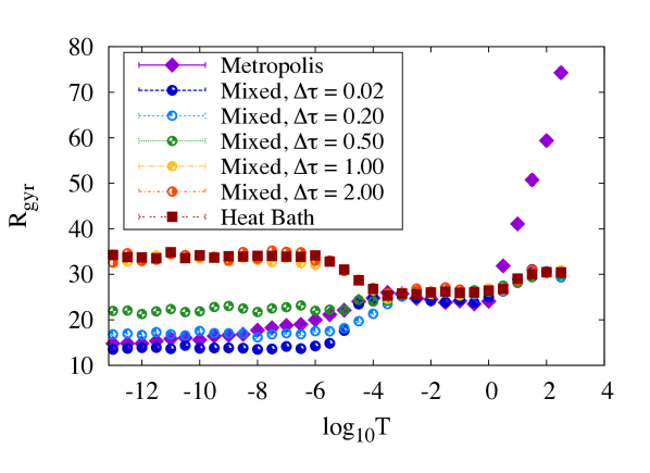
Figure 1: (Color online) Dependence of $R_{gyr}$ on temperature for identical homopolymer chains simulated with different algorithms. Here $\Delta\tau$ is dispersion of Gaussian distribution for generation of $\tau_{\text{new}}$ in mixed algorithm. In conventional Metropolis algorithm the dispersions are $\Delta\kappa=\Delta\tau=0.01$. Length of polymer chain is $N$=100, parameters of the Hamiltonian are the ones from Table I.

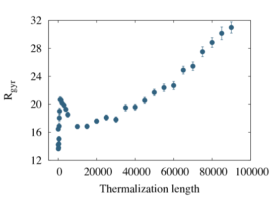
Figure 2: Dependence of $R_{gyr}$ on the thermalization length in Metropolis algorithm. The number of updates, per one step in simulated annealing process (thermalization length), is shown along the horizontal axis. Temperature is $T=10^{-12}$, length of polymer $N$=100, and parameters of Hamiltonian are taken from the Table I.

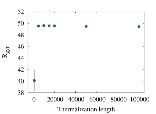
Figure 3: Dependence of $R_{gyr}$ on the thermalization length in Mixed algorithm. The number of updates, per one step in simulated annealing process (thermalization length), is shown along the horizontal axis. Parameters of this run are the same as for the figure 2.

In the sequel the radius of gyration (2) is utilised as the principal observable, to characterise the geometry of the homopolymer chain. Its value is calculated as an average over statistically independent chain configurations, produced during a Monte-Carlo process. In Figure 1 the value of the radius of gyration (2) is compared, as a function of Monte Carlo temperature for a chain with N=100 monomers. The results obtained using the Metropolis algorithm are found to be very different from those obtained using the Heat Bath and Mixed algorithms; for small dispersion $\Delta\tau$ the Mixed algorithm coincides with the Metropolis algorithm. But when $\Delta\tau$ increases, the Mixed algorithm approaches the Heat Bath algorithm as shown in the Figure.

There is no a priori reason why the results for the three algorithms should be different: The stationary distribution is the same, in each of the three algorithms. But it is found that the Metropolis algorithm converges very slowly towards the equilibrium distribution. For this, the dependence of the result on the length of simulation has been analysed. In the case of the Metropolis algorithm, the results are shown in the Figure 2, for $T=10^{-13}$ which is the lowest Monte Carlo temperature value that has been used in the present simulations. As shown in the Figure, $R_{gyr}$ continues to increase with increasing length of thermalization. The Metropolis algorithm approaches the Heat Bath algorithm very slowly, as a function of the simulation time and even at the present, relatively long simulation times the chain is still far from equilibrium distribution.

On the other hand, the results shown in Figure 3 demonstrate that in case of the mixed algorithm the radius of gyration $R_{gyr}$ approaches a fixed value with increasing of the thermalization length. It is concluded that using the present simulation times, the Markovian homopolymer reaches a stationary distribution. Either the Heat Bath algorithm, or alternatively the Mixed algorithm with sufficiently large $\Delta\tau$, should be used to try and describe the thermal equilibrium configurations.

The compactness index $\nu$ i.e. the inverse of the Hausdorff dimension has also been inspected, using the three different algorithms. The results for the Heat Bath algorithm are shown in Figure 4.

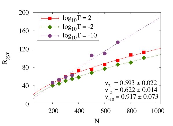
Figure 4: (Color online) Compactness index $\nu$ at different temperatures for a homopolymer chain. Simulation performed with Heat Bath algorithm. Parameters of Hamiltonian are taken from the Table I.

Between $T=100$ and $T=1000$ the value of $\nu$ is essentially temperature independent, and apparently corresponds to the SAW phase. At very low temperatures a transition to the rigid rod state, with $\nu\approx 1$, is observed. This result is in line with the general arguments that are presented in sub-section II.7, on the expected phase structure of the homopolymer model (29), (18).

II.8.5 The final algorithm

On the basis of the results from the test runs, the following improved Heat Bath algorithm is employed in the sequel: The final probability distribution is

$$P=\frac{1}{Z}\exp\{-\beta[H+\sum_{i<j}U(\vec{r}_{i}-\vec{r}_{j})]\}$$ (47)

Here $H$ is the Hamiltonian (29) and $U$ is the potential (37). The Metropolis algorithm is used for acceptance, but with a proposal distribution that coincides with the Heat Bath algorithm: The new values of $\kappa_{i}$ and $\tau_{i}$ are generated using the distributions (40) and (41). The ensuing homopolymer configuration is then accepted, provided it satisfies both the self-avoidance condition (18) and the Metropolis accept-reject condition that utilises the residual energy

$$E_{U}=\sum_{i<j}U(\vec{r}_{i}-\vec{r}_{j})$$ (48)

The acceptance criterion is

$$\exp(-\beta\Delta E_{U})>\lambda$$ (49)

where $\lambda$ is a random number which is uniformly distributed between 0 and 1, and $\Delta E_{U}$ is the change in $E_{U}$ under the update of $\kappa_{i}$ and $\tau_{i}$.

Finally, the algorithm has been calibrated by considering the limit of a truncated Hamiltonian , where the Hamiltonian $H$ is removed and only the attractive potential (37) together with the forbidden volume constraint (18) are retained. The numerical value of $U_{0}$ determines solely the scale of the Monte Carlo temperature $T$, in the present simulations the value $U_{0}=15$ is used. The results are shown in Figure 5.

Figure 5: (Color online) Dependence of $R_{gyr}$ on temperature T for a chain with 100 monomers, in the truncated model. Here $n$ is the number of Monte Carlo updates per one simulated annealing step in temperature (thermalization length). The final algorithm described in paragraph H5 of the section II is used.

A smooth transition is observed in the radius of gyration, from larger values at high temperatures to smaller values at low temperatures.

The Figure 6

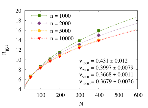
Figure 6: (Color online) Dependence of $R_{gyr}$ on the length of polymer chain $N$ for different thermalization lengths with $T=1$, in the truncated model. The final algorithm is used.

shows how $R_{gyr}$ depends on the length of polymer chain $N$, and fitted to the leading order contribution in (3). The results demonstrate how the equilibrium distribution is reached with a sufficiently long thermalization length, even in the region of low temperatures where the convergence is at its lowest. In particular it is found that the value of the compactness index $\nu$ converges towards the mean field value $1/3$ of the collapsed phase, as shown in Figure 7; the difference between the space filling $\nu=1/3$ and the numerically deduced $\nu\approx$ 0.36 is attributed to the finite size corrections in (3); the available computer power does not enable an identification of the amplitudes $R_{1},...$ or the critical exponents $\delta_{1},...$ in (3) .

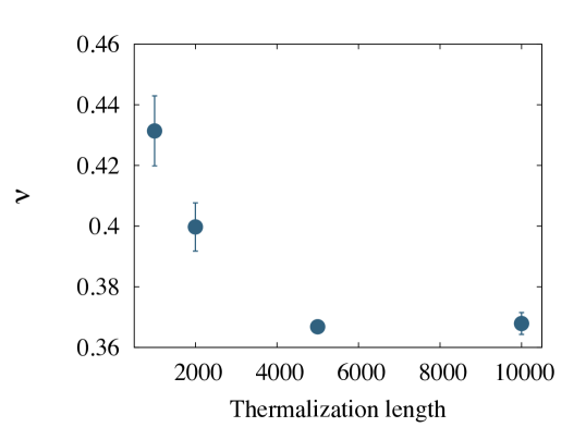
Figure 7: Dependence of compactness index $\nu$ on thermalization length when $T=1$, in the truncated model.

III RESULTS

The present variant of the Heat Bath algorithm has been used in extensive numerical simulations to investigate the phase structure of the homopolymer model (29), (37). The results are summarised in Figures 8-12.

III.1 Effect of parameters

III.1.1 Parameter $U_{0}$

Figures 8-10 describe the properties of the radius of gyration for three representative values of the strength parameter $U_{0}$ in (37),

$$U_{0}\ =\ \left\{\ \begin{matrix}10^{-4}\\ 10^{-2}\\ 10^{-1}\end{matrix}\right.$$ (50)

For the other parameters the values (46) are used. For each value of $U_{0}$, three different characteristic regimes are observed. In the high temperature limit the homopolymer is found in the SAW phase; this is confirmed in Figure 9. When the temperature decreases, the homopolymer enters a regime of decreasing $R_{gyr}$. Finally, there is the low temperature regime where the radius of gyration $R_{gyr}$ has a small value; see Figure 10. The compactness index $\nu$ shows that when the thermalization increases the value of $\nu$ converges towards the values close to $\nu\approx 0.39$ which is indicative of the mean field value $1/3$. This is shown in Figure 11. Again, the difference between the mean field value $\nu=1/3$ and the measured value $\nu\approx 0.36$ is allocated to finite size corrections in (3); the available computer power is not sufficient to deduce the detailed form of these corrections.

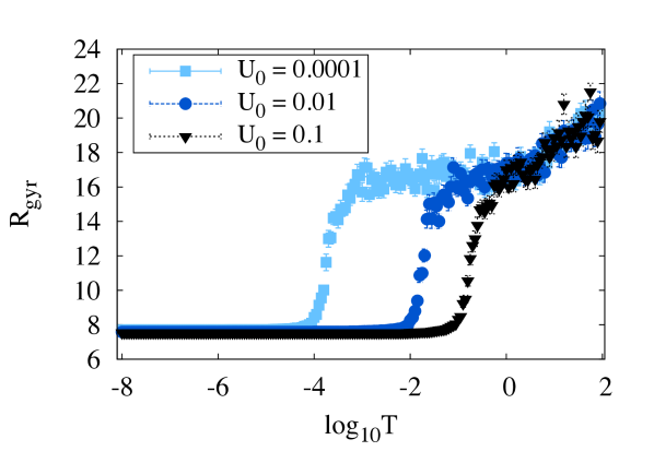
Figure 8: (Color online) Dependence of $R_{gyr}$ on temperature for a chain with 50 monomers. Parameters of the Hamiltonian are taken from the Table I.

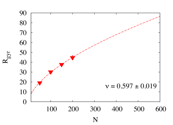
Figure 9: Dependence of $R_{gyr}$ on the length of chain for high temperature $T=10^{1.7}$ and with $U_{0}=0.01$. Parameters of the Hamiltonian are taken from the Table I.

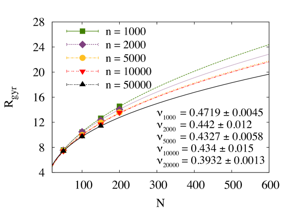
Figure 10: (Color online) Dependence of $R_{gyr}$ on the length of chain for low temperature $T=10^{-6}$ and various thermalization lengths, and with $U_{0}=0.01$. Parameters of the Hamiltonian are taken from the Table I.

Figure 11: Dependence of compactness index $\nu$ on thermalization length. Temperature is equal to $T=10^{-6}$ and $U_{0}=0.01$. Parameters of the Hamiltonian are taken from the Table I.

It is concluded that when the scale for $U_{0}$ exceeds that of $a$ and $c$ the low temperature state is a collapsed configuration.

III.1.2 Parameters $a$ and $c$

According to (36) the classical ground state profile of $\tau_{i}$ remains intact when the parameters $a$ and $c$ are changed in such a manner that the ratio $a/c$ is constant. To study the effect of such a change in $a$ and $c$ at finite temperature, in particular how it conspires with the parameter $U_{0}$, simulations have first been performed with

$$a\ =\ c\ =\ 10^{-2}\ \ \ \ \&\ \ \ \ \ \ U_{0}=10^{-4}$$ (51)

with the values (46) for the remaining parameters. Thus, unlike in the previous simulations now the characteristic scale of the attractive interaction is smaller than that of the torsion angle dependent terms in the Hamiltonian.

The results for the radius of gyration are presented in the Figure 12. At high temperatures the chain is again in the SAW phase. Then, as temperature decreases, there is a transition to a regime akin the intermediate regime shown in Figure 8. Finally, there is a low temperature regime where the chain fluctuates around the classical solution (36). The scale of transition to the low temperature regime is controlled by parameters $a$ and $c$ in Hamiltonian.

It is concluded that when the scale $U_{0}$ of the short-range attractive interaction is smaller than the scale of the parameters $a$ and $c$, the low temperature limit is described by helical structures.

Figure 12: Dependence of $R_{gyr}$ on temperature. The chain has 100 monomers, and parameters ($a,c,U_{0}$) are given in (51).

III.2 Analysis of different phase regimes

The bond and torsion angles form the complete set of local order parameters to probe the phase structure (4), in the case of the present homopolymer model. These order parameters have the following characteristics, in the different regimes that have been analysed in Figures 8-12; the results are summarised in Figures 13-16.

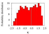
(a)

(b)

Figure 13: Distribution of ($\kappa_{i},\tau_{i}$) in the high temperature SAW phase. Simulation parameters are the same as for the figure 8 ($U_{0}=0.01$), temperature is $T=100$.

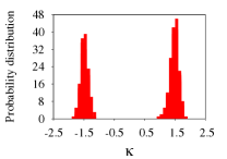
(a)

(b)

Figure 14: Distribution of ($\kappa_{i},\tau_{i}$) in the intermediate transition regime: an example of pseudogap state (see its description in section II.5. Simulation parameters are the same as for the figure 8 ($U_{0}=0.01$), temperature is $T=1$.

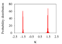
(a)

(b)

Figure 15: Distribution of ($\kappa_{i},\tau_{i}$) in the collapsed phase. It should be observed that the distribution of $\tau_{i}$ is asymmetric, corresponding to broken chirality. Simulation parameters are the same as for the figure 8 ($U_{0}=0.01$), temperature is $T=10^{-7}$.

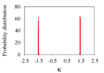
(a)

(b)

Figure 16: Distribution of ($\kappa_{i},\tau_{i}$) in the helical rod-like phase. Simulation parameters are the same as for the figure 12, temperature is $T=10^{-7}$.

In the very high temperature SAW phase, both the bond angle and the torsion angle are subject to large fluctuations; the simulation results are shown in Figure 13. For the bond angles, the values are distributed in the range $0\ \leq\ \ \langle\!\!|\kappa|\!\!\rangle\ \ \leq\ \kappa_{max}\ \sim\ 2.2$. The upper limit reflects the forbidden volume constraint (18). As temperature increases, the values of $\kappa$ become increasingly evenly distributed over this range so that in the $T\to\infty$ limit the distribution is fully uniform; the Figure 13 shows the bond and torsion angle distribution at a generic but high temperature value. It is apparent from this Figure that both angles are disordered.

It is concluded that the SAW phase is a disordered phase.

Next, we observe the intermediate regime takes place between temperature values within the range $10^{-3}<T<10^{1}$ as can be seen in Figures 8 and 12. In this intermediate region the values of the bond angle are found to become ordered. This is shown in Figure 14: The values of $\kappa_{i}$ are thermally fluctuating at around $|\kappa|\approx 1.5$. The values of the torsion angle remain largely disordered. The intermediate region is identified as a pseudogap state, as described in the Introduction.

Finally, there are two different low temperature phases: The collapsed phase shown in Figure 8 where the attractive short-distance interaction dominates and the helical rod-like phase shown in Figure 12 where the attractive short-distance interaction becomes weak.

The distribution of bond and torsion angles in the collapsed phase are displayed in Figure 15. The bond angle is highly ordered around the classical value (36) but the torsion angle remains disordered. However, there is an apparent spontaneous symmetry breaking that has taken place; the double well structure seen in the $\tau$ distribution of Figure 14 has been removed, in a way that resembles the familiar spontaneous symmetry breaking in a $\mathbb{Z}_{2}$ symmetric potential well.

In the helical rod-like phase, both the bond and torsion angles become peaked around the classical values (36). The configurations are akin straight helical rods; a little like e.g. collagen when biologically active. The $\kappa$ distribution reflects the discrete $\mathbb{Z}_{2}$ gauge symmetry. But the $\mathbb{Z}_{2}$ symmetry in the $\tau$ distribution observed in Figure 14 is fully broken.

The transition between the collapsed phase and the helical rod-like phase entails a transitition where the torsion angles become ordered. Due to the very low temperature values involved, the fluctuations are strongly suppressed and a simulation becomes tedious. It is conjectured that, when the temperature is kept in the low temperature regime, an initial helical rod-like structure but with parameter values corresponding to the collapsed phase, is in a glassy phase. Vice versa, an initial collapsed configuration with parameter values in the helical rod-like phase, will eventually become subject to cold denaturation.

III.3 Phase diagram

The homopolymer phase is found to depend on three relevant scales.

– There is the extrinsic temperature scale where the values of $\kappa_{i}$ become ordered. This scale can also be controlled intrinsically, by the parameter $q$ in (29), but the details have not been addressed here.

– There is temperature scale where the values of $\tau_{i}$ become ordered. This scale can be controlled intrinsically, by the parameter ratio $a/c$ in (29).

– Finally, the effects of the scale $U_{0}$ for the short-range attractive interactions have been investigated. This parameter determines an intrinsic scale that controls the transition temperature alternatively to the collapsed phase, or to the helical rod-like phase.

Thus, by changing the relations between the three scales the phase diagram of the homopolymer can be identified; the phase diagram is constructed here in terms of ($T,a,U_{0}$). All the remaining parameters are fixed, and given by the values in Table 1.

The Figure 17 shows the three-dimensional phase diagram in the ($T,a,U_{0}$) space. The Figures 21-21 show various cross-sections, taken at selected values of $U_{0}$ i.e. these Figures show the phase diagram in Figure 17 on the ($a,T$) plane, with different values of $U_{0}$.

Figure 21 shows the phase diagram, for a quite large value of $U_{0}$ (strong coupling) At high temperatures there is the SAW phase. When temperature decreases there is the pseudogap state, that becomes the collapsed phase at low temperatures. Between the pseudogap state and the low temperature collapsed phase there is a $\theta$-regime, or rather a $\theta$-point as it is observed only over a very narrow temperature range.

– Figure 21 displays the phase diagram, when the value of $U_{0}$ is lowered but still relatively large (intermediate but not weak coupling). At high temperatures there is again the SAW phase, followed by the pseudoogap state as the temperature decreases. At low temperatures the pseudogap state becomes converted either to the collapsed phase or to the straight rod phase, depending on the value of the helicity parameter $a$. In addition, there is a range of values of $a$, when a intermediate similar to the $\theta$-regime is observed between the pseudogap state and the straight rod phase. This is the $\eta$-regime. It is notable, that there is a possibility of a 4-critical point involving the pseudogap state, the $\eta$-regime, and the collapsed and straight rod phases.

– Figure 21 shows the phase diagram, as the value of $U_{0}$ becomes further decreased (intermediate but not strong coupling). The collapsed state has entire disappeared, and replaced by the straight rod phase at very low temperatures. The $\eta$-regime displays a periodic structure in the parameter $a$. There appears to be a tri-critical point involving the pseudogap state, the $\eta$-regime and the straight rod phase.

– Finally, in Figure 21 the weak coupling $U_{0}$ phase diagram is displayed. The overall topology of the phase diagram is similar to the one in Figure 21, but with the straight rod phase as the low temperature phase instead of the collapsed phase.

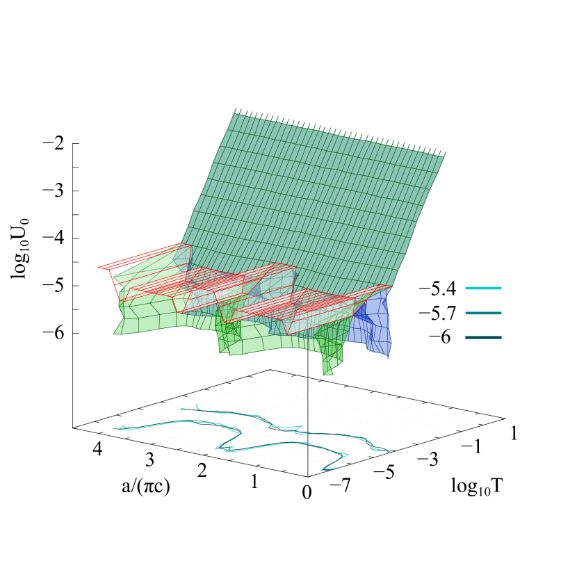
Figure 17: (Color online) The phase diagram on the ($U_{0},T,a$) space. It was obtained for the polymer length $N=100$ using our final algorithm. All parameters in the Hamiltonian except $a$ are fixed according to the Table I.

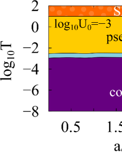
Figure 18: (Color online) A cross-section of the phase diagram in 15 at $U_{0}=10^{-3}$.

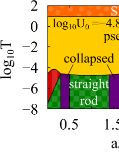
Figure 19: (Color online) A cross-section of the phase diagram in 15 at $U_{0}=10^{-4.8}$.

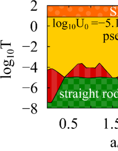
Figure 20: (Color online) A cross-section of the phase diagram in 15 at $U_{0}=10^{-5.1}$.

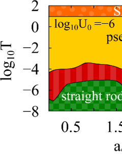
Figure 21: (Color online) A cross-section of the phase diagram in 15 at $U_{0}=10^{-6}$

The Figure 22 shows the phase diagram on the ($U_{0},T$) plane, with helicity fixed. It is notable that there might be a 5-criticality involving the $\eta$- and $\theta$-regimes, the pseudogap state and the collapsed and straight rod phases. However, the detailed investigation of this region of the phase diagram is beyond the capacity of the computer power which is presently available to us.

Figure 22: (Color online) The phase diagram on the ($U_{0},T$) plane, with $a=10^{-4}$.

In summary, it is remarkable how the phase diagram (figures 17-21) is periodic in the helicity parameter $a$ (when $c$ is fixed). Moreover, there is a rapid transition between the helical phase where the compactness index $\nu=1$ and the collapsed phase where $\nu\approx 1/3$ at low temperatures, as shown in Figure 21. There is a pseudogap state that appears as a transition regime, akin the conventional $\theta$-regime, between the collapsed and the SAW phases. For the transition regime between SAW and helical phases shown in Figure 21 there is a pseudogap state that should essentially coincide in its properties with the $\theta$-regime pseudogap state. But due to computational limitations the present analysis is not sufficient to confirm this. There is an apparent 4-critical, even 5-critical point as shown in Figures 21 and 22, but the detailed analysis of this region in the phase diagram needs to be performed using more extensive simulations, which is postponed to a future project. However, it is observed that the potential presence of a 4-critical point in a theoretical context very similar to the present one (i.e. Abelian Higgs model) has been reported in bock-2007

III.4 Heteropolymer and proteins

Finally, it is inquired how the present results could be extended to heteropolymers, to draw conclusions on the potential phase structure of proteins. For this, the effect of perturbations that break the homogeneity of the homopolymer model have been investigated as follows: A collapse has been found to take place when the parameter $U_{0}$ that characterises the strength of self-interaction is larger than the parameters $a$ and $c$ that characterise the torsion angle dependent terms. Thus, a short segment is introduced along the chain, where $U_{0}$ is less than $a$ and $c$. Accordingly, a simulation is performed where a heteropolymer is constructed so that for a short sub-chain of 12 monomers, the values of the parameters $a$ and $c$ is increased from $a=c=10^{-6}$ to $a=c=10^{-2}$, while $U_{0}=10^{-4}$ along the entire chain.

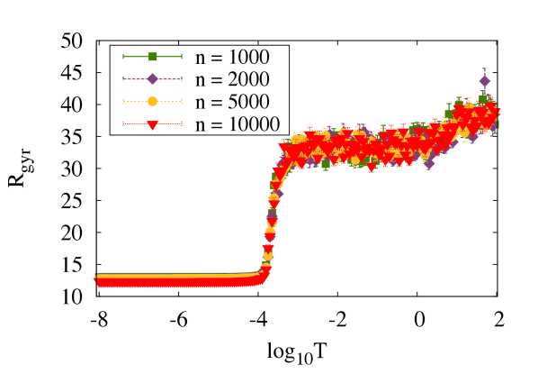
Figure 23: (Color online) Dependence of $R_{gyr}$ on temperature for a heteropolymer chain with 150 monomers Thermalization length $n$ is number of updates per one step of simulated annealing. Parameters of the Hamiltonian and attraction potential are described in the paragraph D of the section III.

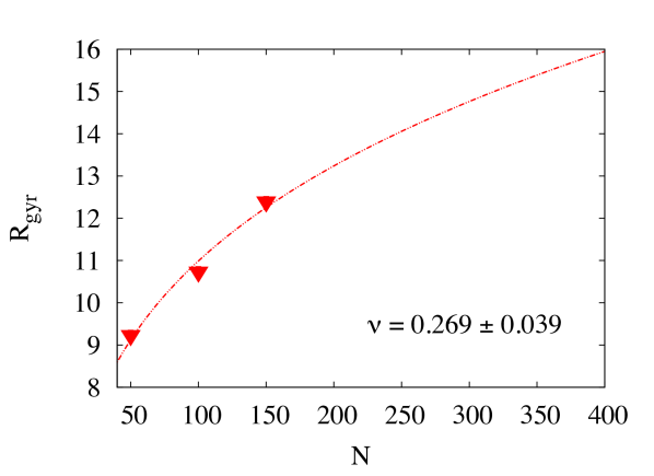
Figure 24: Dependence of $R_{gyr}$ on the length of polymer chain for low temperature $T=10^{-7.5}$. Simulation parameters are the same as for the figure 23.

Results of simulations are presented in Figures 24 and 24, for a chain with 150 monomers. The dependence of $R_{gyr}$ on temperature is shown in figure 24; the phase diagram is very similar to 8. For example, at low temperatures it is found that the compactness index is close to the mean field value $\nu=1/3$ of the collapsed phase. However, the geometry of a configuration in the collapsed phase is different: As shown in Figure 25 a helical structure appears only in that sub-chain where the parameter values $a$ and $c$ have been increased.

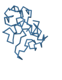
(a)

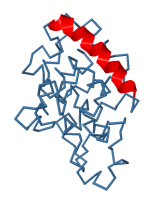
(b)

Figure 25: (Color online) (left) Homopolymer does not display helices in the ground state. (right) Addition of a subchain that breaks homogeneity, gives rise to a helix in the subchain region. Homopolymer configuration was obtained in simulation under the parameters inside the ‘’collapsed” region of the phase diagram (see figure 17). In case of heteropolymer the simulation parameters are the same as for the figure 23, dimensionless temperature $T$ (see paragraph IIH) is equal to $10^{-7.5}$.

IV Summary

The phase structure of chiral homopolymers under varying ambient temperature values have been investigated theoretically, in terms of a universal infrared limit energy function in combination with forbidden volume constraints (self-avoidance) and a short-range attractive interaction between residues. As such, the model should provide a realistic description even in the case of heteropolymers that display an approximatively repeating monomer pattern, provided the scale of the repeat can be considered small in comparison to the chain length. A biologically important example is given by collagen, the most prevalent protein in a human body, in which case the short range attractive interaction models weak hydrophobicity of the amino acids.

It is found that the phase diagram displays a high level of complexity, in terms of the parameters that control the helicity, and the strength of the attractive interaction. In particular, the low energy phase is either like a linear one dimensional straight rod, or a space filling collapsed configuration. At intermediate temperatures, there is a state which can be identified as an example of the pseudogap state, and there are also intermediates that are more like the conventional $\theta$-regime. It is possible that these regimes merge, in the thermodynamical limit, at least for some range of parameter values. However, the possibility of the existence of 4-critical, even 5-critical points in the phase diagram is also proposed, but can not be confirmed with presently available computer power.

The extension of the present approach to investigate properties of proteins and other heteropolymers remains a challenge to future research.

V Acknowledgements

AJN acknowledges support from Region Centre Recherche d^′Initiative Academique grant, Vetenskapsrådet, Carl Trygger’s Stiftelse för vetenskaplig forskning, and Qian Ren Grant at BIT. The work of MU was supported by the DFG grant SFB/TR-55 and by Grant RFBR-14-02-01261-a. Numerical calculations were performed at the ITEP computer systems “Graphyn” and “Stakan” and at the supercomputer center of Moscow State University. AJN thanks A. Sieradzan and Nevena Ilieva for discussions. We dedicate our research to the memory of M. Polikarpov, a close colleague, mentor and teacher without whom our collaboration would not be. Thank you, Misha.

- (1) A. J. Heeger, Rev. Mod. Phys. 73 (2001) 681.
- (2) A. J. Niemi, G. W. Semenoff, Phys. Rep. 135 (1986) 99.
- (3) J. Hiraki, Journ. Antib. Antif. Ag. 23 (1995) 349.
- (4) C. Li, D. F. Yu, A. Newman, F. Cabral, C. Stephens, N. R. Hunter, L. Milas, S. Wallace, Cancer Res. 58 (1998) 2404.
- (5) P. G. De Gennes, Scaling Concepts in Polymer Physics (Cornell University Press, Ithaca, 1979).
- (6) A. Yu. Grosberg, A. R. Khokhlov Statistical Physics of Macromolecules (AIP Series in Polymers and Complex Materials, Woodbury, 1994).
- (7) L. Schäfer, Excluded Volume Effects in Polymer So- lutions, as Explained by the Renormalization Group (Springer Verlag, Berlin, 1999).
- (8) A. J. Niemi, Phys. Rev. D67 (2003) 106004.
- (9) U. H. Danielsson, M. Lundgren, A. J. Niemi, Phys. Rev. E82 (2010) 021910.
- (10) S. Hu, Y. Jiang, A. J. Niemi, Phys. Rev. D87 (2013) 105011.
- (11) T. Ioannidou, Y. Jiang, A. J. Niemi, Phys. Rev. D90 (2014) 025012.
- (12) A. J. Niemi, Theor. Math. Phys. 181 (2014) 1235.
- (13) A. J. Niemi, arXiv:1412.8321 [cond-mat.soft].
- (14) V. J. Emery, S. A. Kivelson, Nature 374 (1995) 434.
- (15) J. Corson, R. Mallozzi, J. Orenstein, J. N. Eckstein, I. Bozovic, Nature 398 (1999) 221.
- (16) N. Mannella, et.al. Nature 438 (2005) 474.
- (17) H. Kleinert, E. Babaev, Phys. Lett. B438 (1998) 311.
- (18) K. Zarembo, JETP Letters 75 (2002) 59.
- (19) L. P. Kadanoff, Physics 2 (2006) 263.
- (20) K. G. Wilson, Phys. Rev. B4 (1971) 3174.
- (21) K. G. Wilson, J. Kogut, Phys. Repts. 12 (1974) 75.
- (22) B. Widom, J. Chem. Phys. 43 (1965) 3892.
- (23) M. E. Fisher, Rev. Mod. Phys. 46 (1974) 597.
- (24) P. G. De Gennes, Phys. Lett. 38A (1972) 339.
- (25) J. C. LeGuillou, J. Zinn-Justin, Phys. Rev. B21 (1980) 3976.
- (26) B. Li, N. Madras, A. Sokal, Journ. Stat. Phys. 80 (1995) 661.
- (27) S. Hu, M. Lundgren, A. J. Niemi, Phys. Rev. E83 (2011) 061908.
- (28) A. Krokhotin, A. Liwo, A. J. Niemi, H. A. Scheraga Journ. Chem. Phys. 137 (2012) 035101.
- (29) M. L. Huggins, Journ. Chem. Phys. 9 (1941) 440.
- (30) P. J. Flory, Journ. Chem. Phys. 9 (1941) 660.
- (31) P. J. Flory, Principles of Polymer Chemistry (Cornell University Press, Ithaca, 1953).
- (32) M. Bock, M. N. Chernodub, E.-M. Ilgenfritz, A. Schiller Phys.Rev. B76 (2007) 184502.
- (33) K. Hinsen, S. Hu, G. R. Kneller, A. J. Niemi Journ. Chem. Phys. 139 (2013) 124115.
- (34) S. Coleman, E. Weinberg Phys. Rev. D7 (1973) 1888.
- (35) M. N. Chernodub, L. D. Faddeev, A. J. Niemi, JHEP 12 (2008) 014.
- (36) L. D. Faddeev, L. A. Takhtajan, Hamiltonian methods in the theory of solitons (Springer Verlag, Berlin, 1987).
- (37) M. J. Ablowitz, B. Prinari, A. D. Trubatch, Discrete and Continuous Nonlinear Schrödinger Systems (London Mat. Soc. Lect. Note Series 302, London, 2003).
- (38) N. Molkenthin, S. Hu, A. J. Niemi, Phys. Rev. Lett. 106 (2011) 078102.
- (39) M. Chernodub, S. Hu, A. J. Niemi, Phys. Rev. E82 (2010) 011916.
- (40) R. Peierls, Proc. Phys. Soc. 52 (1940) 34.
- (41) F. Nabarro, Proc. Phys. Soc. 59 (1947) 256.
- (42) F. Nabarro, Mat. Sci. Eng. (1997) A234 67.
- (43) A. K. Sieradzan, A. J. Niemi, X. Peng, Phys. Rev. E90 (2014) 062717.
- (44) B. A. Berg, Markov Chain Monte Carlo Simulations and Their Statistical Analysis (World Scientific, Singapore, 2004).
- (45) A. Krokhotin, M. Lundgren, A. J. Niemi, X. Peng, J. Phys.: Condens. Matter 25 (2013) 325103.
- (46) P. L. Freddolino, C. B. Harrison, Y. Liu, K. Schulten, Nature physics 6 (2010) 751.
- (47) K. A. Dill and J. K. MacCallum, Science 338 (2012) 1042.
- (48) S. Piana, J. L. Klepeis, D. E. Shaw, Curr. Opin. Struc. Biol. 24 (2014) 98.
- (49) D. E. Shaw, et al., Communications of the ACM 51.7 (2008) 91
- (50) D. E. Shaw, et al., High Performance Computing Networking, Storage and Analysis, Proceedings of the Conference IEEE (2009).