Comparative study of nonclassicality, entanglement, and dimensionality of multimode noisy twin beams
Abstract
The nonclassicality, entanglement, and dimensionality of a noisy twin beam are determined using a characteristic function of the beam written in the Fock basis. One-to-one correspondence between the negativity quantifying entanglement and the nonclassicality depth is revealed. Twin beams, which are either entangled or nonclassical (independent of their entanglement), are observed only for the limited degrees of noise, which degrades their quantumness. The dimensionality of the twin beam quantified by the participation ratio is compared with the dimensionality of entanglement determined from the negativity. Partitioning of the degrees of freedom of the twin beam into those related to entanglement and to noise is suggested. Both single-mode and multimode twin beams are analyzed. Weak nonclassicality based on integrated-intensity quasidistributions of multimode twin beams is studied. The relation of the model to the experimental twin beams is discussed.
pacs:
42.65.Lm,42.50.Ar,03.67.Mn,42.65.YjI Introduction
The question whether a given state cannot be described within a classical theory has been considered one of the most serious since the early days of quantum physics Einstein05 ; Einstein35 ; Schrodinger35 (for a review see, e.g., Ref. Perina1994Book ). Nonclassicality and entanglement, which is one of the nonclassicality manifestations, are the most important properties of optical fields studied in quantum optics. Such fields have no classical analogs and as such they have been found interesting for many reasons. Nonclassical properties of such fields have been found useful both for elucidating the principles of quantum mechanics and in various applications including, e.g., quantum information processing NielsenBook , quantum metrology Migdall1999 ; Giovannetti2011 ; PerinaJr2012a , and highly-sensitive measurements Vahlbruch10 .
From both the theoretical and the experimental points of view, the nonlinear process of parametric down-conversion, in which photon pairs are generated, has played an important role here from the beginning of investigations MandelBook ; Perina1991Book ; Perina1994Book ; WallsBook . Its individual photon pairs have been exploited in many fundamental experiments testing nonclassical behavior predicted by quantum physics Bouwmeester1997 ; Weihs1998 . It has also allowed the generation of more intense fields having their electric-field amplitude quadratures squeezed below the vacuum level Luks1988 ; Lee1990 ; Lvovsky2009 , exhibiting sub-shot-noise correlations Jedrkiewicz2004 ; Bondani2007 or having sub-Poissonian photon-number statistics PerinaJr2013b ; Lamperti2014 ; Lamperti2014a .
In quantum optics, the definition of nonclassicality is based upon the Glauber-Sudarshan representation Glauber63 ; Sudarshan63 ; Perina1991Book of the statistical operator of a given field. The commonly accepted formal criterion for distinguishing nonclassical states from classical ones is expressed as follows DodonovBook ; VogelBook ; MandelBook ; Perina1991Book : A quantum state is nonclassical if its Glauber-Sudarshan function fails to have the properties of a probability density. Alternatively, several operational criteria for nonclassicality of either single-mode DodonovBook ; VogelBook ; Richter02 or multimode Miran10 ; Bartkowiak11 ; Allevi2013 fields have been revealed. Their derivations are based either on field’s moments Vogel08 ; Miran10 ; Allevi2013 or on direct reconstruction of quasidistributions of integrated intensities Haderka2005a ; PerinaJr2012 ; PerinaJr2013a . Also, criteria derived from the majorization theory have been found Lee1990a ; Verma2010 .
Entanglement (or inseparability) is a special nonclassical property that describes quantum correlations among (in general) several subsystems that cannot be treated by the means of classical statistical theory Horodecki09review . Various approaches have been developed for discrete and continuous variables to reveal entanglement. This property has been exploited in suggesting an entanglement criterion and the related entanglement measure (referred to as the negativity) based upon the partial transposition of a statistical operator Peres96 ; Horodecki97 ; Zyczkowski98 ; Vidal02 . Another approach has been based on the violation of the Bell inequalities written for different mean values including the measurement on both parts of a bipartite system CHSH . Also, a method using positive semi-definite matrices of fields’ moments of different orders Shchukin05 ; Miran09 has been found to be very powerful. We would like to stress at this point that entanglement is a very crucial tool in today’s quantum information processing.
In this contribution, we study nonclassicality by applying the Lee nonclassical depth Lee91 as well as entanglement via the negativity Zyczkowski98 ; Vidal02 for (in general) noisy twin beams of different intensities. Such fields occur under real experimental conditions in which a nonlinear crystal generates both photon pairs and individual single photons (noise). Nevertheless, the signal and idler fields together form a bipartite quantum system. We note that entanglement and nonclassicality of twin beams generated by down-conversion seeded by thermal light have been analyzed in Refs. Degiovanni2007 ; Bondani2008 ; Degiovanni2009 . In this case, noise present in the incident thermal fields participates in the nonlinear process and generation of photon pairs. This weakens its detrimental effect on entanglement and nonclassicality of twin beams and allows us to have entangled twin beams with a larger amount of noise.
Here we also study the problem of entanglement dimension via the negativity for general twin beams and the Schmidt number for noiseless twin beams in a pure state. Namely, we estimate how many degrees of freedom of two fields comprising a twin beam are entangled based on the results of Ref. Eltschka13 for axisymmetric states. On the other hand, the participation ratio Zyczkowski99 determined from the reduced statistical operator of the signal (or idler) field gives the number of degrees of freedom in this field serving to describe both entanglement and noise. It varies from (for a pure state ) to for the completely mixed state . We note that the participation ratio gives an effective number of states in the mixture implied by the property that it is a lower bound for the rank of . Moreover, the logarithm of is the von Neumann–Renyi entropy of second order Zyczkowski99 . The inverse of the participation ratio is referred to as the purity (or linear entropy). Various methods for direct measuring the Schmidt number (even without recourse to quantum tomography) were proposed for noiseless twin beams (see, e.g., Refs. Fedorov04 ; Fedorov07 ; Chan07 ; Pires09 ; Bartkiewicz13 ). The method of Ref. Chan07 was recently realized experimentally Just13 . We note that the negativity can also be measured without applying quantum tomography as described, e.g., for two polarization qubits using linear optical setups Bartkiewicz14 ; Bartkiewicz14a .
The paper is organized as follows. In Sec. II, the model of parametric down-conversion providing an appropriate statistical operator of a twin beam is presented. Entanglement of the twin beam is addressed in Sec. III using the negativity. The nonclassical depth is introduced in Sec. IV to quantify nonclassicality. The relation between the negativity and the nonclassical depth is also discussed in Sec. IV. The dimensionality of a twin beam described by the participation ratio together with the entanglement dimensionality described by the negativity is analyzed in Sec. V. Properties of -mode twin beams are discussed in Sec. VI. Section VII is devoted to experimental multimode twin beams containing also noise embedded in independent spatiotemporal modes. Conclusions are drawn in Sec. VIII.
II Quantum model of a twin beam
To describe the generation of a single-mode twin beam by parametric down-conversion, we adopt the approach based on the Heisenberg equations derived from the appropriate nonlinear Hamiltonian Perina1991Book ,
| (1) |
where and represent the annihilation (creation) operators of the signal and idler field, respectively, and is a real coupling constant that is linearly proportional both to the quadratic susceptibility of a nonlinear medium and to the real pump-field amplitude. The interaction time is denoted , () is the pump-field frequency (phase), and and stand for the signal- and idler-field frequencies, respectively. The law of energy conservation provides the relation . H.c. is the Hermitian conjugated term. In a real nonlinear process, also noise occurs. It can be described by the Langevin forces belonging to a reservoir of chaotic oscillators with mean number of noise photons .
The Heisenberg-Langevin equations corresponding to the Hamiltonian are written as
where the constant () describes damping in the signal (idler) field. The Langevin operators (for ) have the properties
| (3) |
where stands for the Kronecker symbol.
Using the interaction representation [] and neglecting damping together with the Langevin forces, the solution of Eq. (II) attains the form
| (4) |
in which and .
Statistical properties of the twin beam are then described by the normal characteristic function defined as
| (5) |
where denotes the trace. Using the solution given in Eq. (4), the normal characteristic function attains the Gaussian form Perina05 ,
| (6) | |||||
in which and denote independent complex variables. For the undamped and noiseless case, we have . Also the mean number of the generated photon pairs is determined as . When damping and noise are also considered Perina05 , the parameters (for ) contain additional noise contributions characterized by the parameters and , i.e., and . Whereas the parameter gives the mean number of photon pairs, the parameters and correspond to the mean number of noise photons coming from the signal- and idler-field reservoirs, respectively. On the other hand, the parameter describing mutual correlations between the signal and idler fields is not influenced by the noise since .
The statistical operator of the twin beam then acquires the form Perina1991Book
| (7) |
In Eq. (7), denotes an anti-normal characteristic function and symbol means normal ordering of field operators.
Performing integration in Eq. (7) we express the statistical operator in the form
| (8) | |||||
where . The parameters introduced in Eq. (8) are related to anti-normal ordering of field operators and are given as with . Decomposing the statistical operator in the Fock-state basis we finally arrive at the formula
III Negativity of the twin beam
The negativity of a mixed bipartite system defined on the basis of the Peres-Horodecki criterion for a partially transposed statistical operator Peres96 ; Horodecki97 ; Vidal02 is useful for quantifying the entanglement of the twin beam. It can be expressed as
| (11) |
using the trace norm of the partially transposed statistical operator . The negativity essentially measures the degree at which fails to be positive. As such it can be regarded as a quantitative version of the Peres-Horodecki criterion for separability Peres96 ; Horodecki97 . According to Eq. (11), the negativity is given as the absolute value of the sum of the negative eigenvalues of . It vanishes for separable states. It is worth noting that the negativity is an entanglement monotone and so it can be used to quantify the degree of entanglement in bipartite systems. Moreover, the negativity does not reveal bound entanglement (i.e., nondistillable entanglement) in systems more complicated than two qubits or qubit-qutrit Horodecki09review .
To determine the negativity we consider the eigenvalue problem for the partially transposed statistical operator . The statistical operator expressed in the Fock-state basis attains a characteristic block structure. The smallest block has dimension 2 and each successive block has dimension larger by 1. For a given one has a block of dimension . Such a block represents a matrix of isolated states; the sum of indices of their statistical operators equals ,
| (12) |
It can be shown that eigenvalues of a block of dimension can be expressed as using the eigenvalues and of a block with dimension 2:
| (13) |
The negative eigenvalues can only be those containing odd powers of . They form a geometric progression whose elements can be summed to arrive at the formula for the negativity :
| (14) |
Expressing parameters , , and in Eq. (14) in terms of parameters , , and , we arrive at the formula
| (15) | |||||
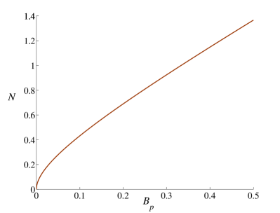
Equation (15) simplifies considerably for noiseless twin beams:
| (16) |
According to Eq. (16), all noiseless twin beams are entangled. The more intense the noiseless twin beams are, the more entangled the signal and idler fields are (see Fig. 1).
The presence of noise in a twin beam can even completely destroy entanglement, as the analysis of Eq. (15) shows. Indeed, the condition for entanglement can be rewritten using Eq. (15) as follows:
| (17) |
Condition (17) cannot be fulfilled for any value of provided that . Thus, the twin beam can be entangled only when
| (18) |
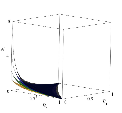
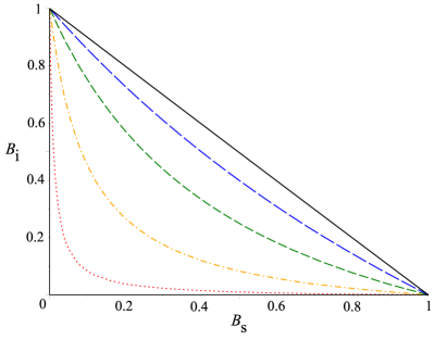
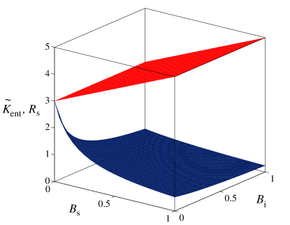
The behavior of the negativity of noisy twin beams dependent on the noise parameters and is illustrated in Fig. 2 for several values of the mean photon-pair number . It holds in general that the greater the value of the mean photon-pair number , the greater the value of the negativity . This can be explained as follows. The more intense twin beams, with their thermal statistics, are effectively spread over a larger number of the Fock states. This naturally results in the larger effectively populated Hilbert spaces used to describe the entanglement. The greater value of the negativity means a greater effective number of the paired modes building the entanglement, i.e., a greater value of the entanglement dimensionality, as defined in Sec. V. Also, the greater the value of the mean photon-pair number , the larger the amount of overall noise acceptable in an entangled twin beam (see Fig. 3). The curves plotted in Fig. 3 indicate that entanglement is more resistent to noise when the noise is distributed in the signal and idler fields asymmetrically. We note that separable states (i.e., with ) contain, in general, paired, signal, and idler noisy contributions. However, the noisy contributions are sufficiently strong to suppress the “entangling power” of the photon-pair contribution and so the state effectively behaves as a classical statistical mixture of the signal and idler fields.
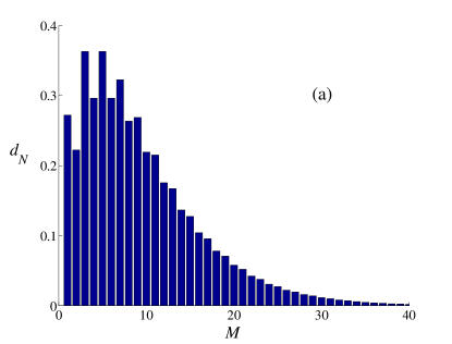
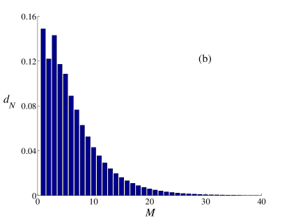
The decomposition of the partially transposed statistical operator into blocks in its matrix representation and the fact that a block (subspace) with dimension describes only states with up to photons in the signal (and also idler) field can be used to define the distribution of the negativity fulfilling the normalization condition
| (19) |
For a given , the element of this distribution is given as the sum of the absolute values of the negative eigenvalues belonging to the block of dimension . The distribution of the negativity provides insight into the internal structure of entanglement. It tells us how entanglement is distributed in the Liouville space of statistical operators. Typical distributions of the negativity for noiseless as well as noisy twin beams are plotted in Fig. 4. A teeth-like structure occurs for smaller numbers in noiseless twin beams. Noise tends to suppress this structure, as is evident from the comparison of the distributions plotted in Figs. 4(a) and 4(b). We note that the densities of the negativity have already been introduced for bipartite entangled states composed of a qubit and continuum of states Luks2012 ; Perinova2014 as well as two continua of states.
IV Nonclassical depth of the twin beam
To quantify nonclassicality of the twin beam we apply the nonclassical depth Lee91 derived from the threshold value of the ordering parameter at which the joint signal-idler quasidistribution of integrated intensities becomes nonnegative Perina05 ; PerinaJr2013a . We adopt the definition . We note that the joint signal-idler quasidistribution of integrated intensities attains negative values for for which . The threshold value can easily be obtained from the condition , which determines the point of the transition between quantum and classical single-mode twin beams PerinaJr2013a . This results in the following formula for the nonclassical depth :
| (20) |
Assuming noiseless twin beams, Eq. (20) simplifies to
| (21) |
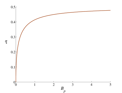
According to Eq. (21), all noiseless twin beams are nonclassical. The greater the mean photon-pair number , the greater the value of the nonclassical depth (see Fig. 5). This depth reaches its greatest value, 1/2, in the limit of an infinitely intense twin beam (). We note that corresponds to symmetrical ordering of the field operators.
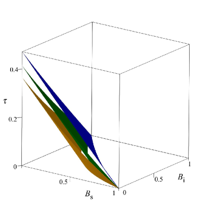
On the other hand, and according to Eq. (20), noise only degrades nonclassical behavior of a twin beam, as documented in Fig. 6. If the noise is equally distributed in the signal and idler fields (), the nonclassical depth determined along Eq. (20) gives the mean number of noise photons needed for suppressing the nonclassicality of the twin beam. So, the larger the value of the nonclassical depth is, the more nonclassical the field is. On the other hand, formal application of Eq. (20) to classical noisy twin beams results in negative values of the nonclassical depth . Their absolute value can be considered a measure of classicality of noisy twin beams in the sense that it quantifies the mean number of photon pairs needed to transform a classical twin beam into the classical-quantum boundary .
Condition for the transition from quantum to classical twin beams applied to Eq. (20) results in the same relation among parameters , , and as derived in Eq. (17) for the boundary between entangled and separable twin beams. Thus, entangled twin beams are nonclassical, whereas separable twin beams are classical. This means that nonclassical twin beams may contain on average only less than one noise photon (). We note that inequality (17) represents the Simon criterion for nonclassicality of Gaussian states as shown in Ref. Perina11 .
Comparison of Eqs. (16) and (21) made for noiseless twin beams reveals a simple relation between the negativity and the nonclassical depth :
| (22) |
Direct calculation based on Eqs. (15) and (20) then confirms that relation (22) holds even for a general noisy twin beam. We thus have a one-to-one correspondence between the value of the negativity and the value of the nonclassical depth . Moreover, according to Eq. (22) the negativity is an increasing function of the nonclassical depth , and vice versa (see Fig. 7). There exists a deep physical reason for this correspondence. The nonlinear process emits photons in pairs into the signal and idler fields, which creates entanglement between these fields. It is this entanglement that gives rise to nonclassical properties of twin beams, as the classical statistical optics is unable to describe pairing of photons appropriately.
V Dimensionality of the twin beam
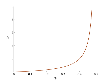
Three different numbers are needed to determine the dimensionality of a general noisy twin beam. The dimensionality of entanglement gives the number of degrees of freedom constituting the entangled (paired) part of the twin beam. We also need additional degrees of freedom to characterize the noisy parts of the twin beam. As the amount of noise is, in general, different in the signal and idler fields, we have independent participation ratios and for both fields. The entanglement dimensionality for bipartite states with axisymmetric statistical operators can be given in terms of the negativity by a simple formula Eltschka13 :
| (23) |
Strictly speaking, it is the least integer that gives a lower bound to the number of entangled dimensions between entangled subsystems (paired modes) of Eltschka13 . According to Eq. (23), the entanglement dimensionality equals 1 for separable states (). It linearly increases with the negativity . As the noise described by the mean noise photon numbers and decreases the values of the negativity , it also decreases the values of the entanglement dimensionality . We note that, for pure states, the Schmidt number is also a good quantifier of the entanglement dimension Law04 ; Gatti2012 ; Chekhova2015 . The Schmidt decomposition of pure states accompanied by convex optimization can even be applied for quantifying the entanglement dimension of mixed entangled states Horodecki09review .
On the other hand, the noise present in the signal and idler fields requires additional degrees of freedom for its description. These degrees of freedom are, together with those reserved for describing entanglement, determined by the participation ratios and derived from the signal- and idler-field reduced statistical operators and , respectively Gatti2012 ; Horoshko2012 :
| (24) |
Equation (10), giving the matrix elements of the statistical operator , guarantees a diagonal form of the reduced statistical operators and of the signal and idler fields, respectively. In this case, Eq. (24) can be rewritten in the form
| (25) |
Using Eq. (10) the matrix elements can be written as
| (26) |
Substituting Eq. (26) into Eq. (25) we obtain a simple formula for the participation ratio :
| (27) |
The same considerations made for the signal field apply also to the idler field.
To find the relation between the entanglement dimensionality and the participation ratios and we consider for a while the noiseless twin beams in pure states. In this case, the elements of the reduced statistical operator , written in Eq. (26), immediately give the squared Schmidt coefficients Pires09 . Combining Eqs. (16), (23), and (27) we arrive at the formula
| (28) |
Equation (28) shows that, excluding weak noiseless twin beams, . This means that the definitions of the entanglement dimensionality and participation ratio set different boundaries for the Schmidt coefficients included in the approximative description of a noiseless twin beam with the wave function
| (29) |
Using Eq. (10), the coefficients in Eq. (29) are obtained in the form
| (30) |
which is in agreement with the thermal photon-number statistics of the signal (or idler) field. We note that the ratio of boundary coefficients is given by the expression . When .
To compare the values of entanglement dimensionality and the participation ratio for general twin beams we have to eliminate the effect of different boundaries set by different definitions, as revealed by considering the pure states. Using the formulas derived for noiseless twin beams, we introduce the modified entanglement dimensionality as follows:
| (31) |
Definition (31) of the modified entanglement dimensionality guarantees that the values of modified entanglement dimensionality and participation ratios and of noiseless twin beams are equal.
The values of the modified dimensionality of entanglement and the signal-field participation ratio are compared in Fig. 8 for the mean photon-pair number . Whereas the values of the modified entanglement dimensionality decrease with increasing values of the mean noise photon numbers and , the values of the signal-field participation ratio increase with increasing values of the mean signal-field noise photon number . We note that the values of the signal-field participation ratio are greater than those of the modified entanglement dimensionality even for , as the presence of noise in the idler field () degrades entanglement.
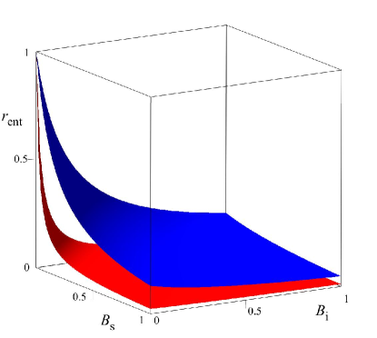
The relative contribution of the degrees of freedom used for describing entanglement in a twin beam is an important characteristic. This contribution can be quantified via the coefficient defined as follows:
| (32) |
As shown in Fig. 9, the greater the values of the mean noise photon numbers and , the smaller the values of the coefficient . The comparison of surfaces of the coefficient drawn for the mean photon-pair numbers and in Fig. 9 reveals seemingly paradoxical behavior. The values of the coefficient decrease with increasing values of the mean photon-pair number . This behavior, however, naturally originates in fragility of entanglement with respect to the noise. More intense twin beams (with greater values of ) are less resistant to a given amount of noise compared to low-intensity twin beams. This is explained by the larger dimensions of the effectively populated Hilbert spaces of more intense twin beams and, thus, the more complex structures of their entanglement. As a consequence, relatively higher numbers of degrees of freedom serving to describe entanglement in more intense noiseless twin beams are “released” by the noise and enlarge the noise parts of twin beams.
Alternatively to the participation ratio , we may apply the von Neumann entropy of a reduced statistical operator. Taking into account the diagonal form of the signal-field reduced statistical operator with the elements written in Eq. (26), the signal-field entropy is in general determined along the formula
| (33) |
Considering the specific form of matrix elements given in Eq. (26), the formula for entropy attains the form
| (34) | |||||
stands for natural logarithm. Combining Eqs. (25) and (34), the entropy is revealed as an increasing function of the participation ratio :
| (35) |
Analogous formulas for the idler-field entropy can easily be derived. The general dependence of entropy on the participation ratio is plotted in Fig. 10.
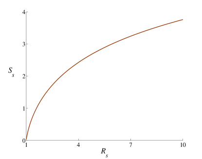
We would like to note that the entropy serves as a good measure of the entanglement for pure states.
VI Twin beam composed of modes
In real experiments, twin beams are rarely composed of only one paired spatiotemporal mode PerinaJr2013a ; Allevi2013 . We note that a twin beam composed of one paired mode represents an ideal field from the experimental point of view Perez14 . For this reason, we consider a multimode twin beam containing independent identical single-mode twin beams. Its statistical operator is given as using the statistical operator written in Eq. (8). There are four parameters characterizing the twin beam: number of modes, mean photon-pair number , mean signal-field noise photon number , and mean idler-field noise photon number . We note that such an -mode twin beam represents a good approximation of a real twin beam when all spatiotemporal modes participating in the nonlinear interaction are detected.
The considered physical quantities behave differently with respect to the number of modes. It has been shown in Refs. Perina05 and PerinaJr2013a that the nonclassical depth does not depend on the number of modes. On the other hand, the multimode negativity , , as well as the participation ratios , for , are multiplicative. We note that the form of the multimode negativity originates in the multiplicative property of the trace norm and its relation to the negativity expressed in Eq. (11) Vidal02 . In fact, the multimode negativity coincides with the entanglement dimensionality defined in Eq. (23) for a single-mode twin beam. The multimode entropies , , are then additive. To reveal similar relations among the studied quantities as has been done for single-mode twin beams, we have to define suitable quantities derived from those considered above. Defining the logarithmic negativity and the logarithmic participation ratios , , we replace the multiplicative quantities with the additive ones. Introducing the logarithmic negativity , logarithmic participation ratios , and entropies related per one mode,
| (36) |
with , we reveal the suitable quantities. The quantities defined in Eq. (36) together with the nonclassical depth behave qualitatively in the same way as those defined for single-mode twin beams discussed above. Especially, the logarithmic negativity per mode is an increasing function of the nonclassical depth . Also, the entropy per mode is an increasing function of the logarithmic participation ratio per mode, .
VII Experimental multimode twin beams
Real experimental multimode twin beams have a more complex structure than that discussed in Sec. VI Haderka2005a ; PerinaJr2013a ; Allevi2013 . The reason is that the spatiotemporal modes of twin beams are shared by the signal and idler fields and so they can be broken before or during the detection owing to spectral and/or spatial filtering. As a consequence, real multimode twin beams are composed of three components PerinaJr2013a ; PerinaJr2012a . A paired component describes photons embedded in spatiospectral modes detected by both signal- and idler-field detectors. A noise signal (idler) component then describes photons occurring in signal (idler) spatiotemporal modes that originate in filtering of the idler (signal) field. If we assume for simplicity that the paired component is ideal, i.e., without noise, we need six parameters to describe a real twin beam. Each component is characterized by the number of modes and mean photon-pair (or noise photon) number . The statistical operator of the experimental twin beam can be expressed as
| (37) |
using single-mode statistical operators , , and of the photon-pair, noise signal, and noise idler components. In Eq. (37), , , and give the numbers of equally populated modes with the mean numbers , , and of photon pairs per mode, respectively.
Entanglement in the experimental twin beam is created only by its paired component and as such it can be quantified by the logarithmic negativity introduced in Sec. VI. The noise components do not contribute to entanglement on one side, and they do not degrade entanglement on the other side. This is qualitatively different from the case of multimode twin beams discussed in Sec. VI and containing noise in paired spatiotemporal modes.
Nonclassicality can be quantified by a multimode generalization of nonclassical depth introduced in Ref. Lee91 for a single-mode field. In a multimode twin beam, we may first determine the standard nonclassical depths for each single-mode field, included either in the paired part of the twin beam or in the noisy signal and idler parts of the twin beam. Then we can take either or to quantify the multimode nonclassical depth . In the first case, the nonclassical depth of the experimental multimode twin beam is just given by the nonclassical depth of a paired mode. The second case is physically more interesting, as the value of is linearly proportional to the minimum amount of additional noise needed to conceal nonclassicality of the multimode state. In this case, we have, for the experimental multimode twin beams,
| (38) |
Using the logarithmic negativity defined in Sec. VI and the nonclassical depth , one-to-one correspondence between the entanglement and the nonclassicality is obtained also for -mode twin beams.
On the other hand, the concept of weak nonclassicality Arvind1997 ; Arvind1998 ; DodonovBook is also useful for the experimental multimode twin beams considered to be composed of one effective paired (macro)mode. The joint quasidistribution of the integrated intensities and of the signal and idler fields, respectively, describes the properties of this effective paired mode Perina1991Book . As no information about the phase is encoded in this simplified effective description, we may only determine the nonclassical intensity depth quantifying nonclassicality, which demonstrates itself by negative values of the marginal quasidistribution of integrated intensities. We have to emphasize that the nonclassical intensity depth is only a nonclassicality witness or parameter, which reveals nonclassicality solely in photon-number statistics. Contrary to this, the nonclassical depth is a genuine and commonly used nonclassicality measure. We note that te standard nonclassicality quantified by reveals both strongly and weakly nonclassical states Arvind1997 ; Arvind1998 . From this point of view is a strong tool or criterion. On the other hand, detects only strongly nonclassical states; i.e., it is a weak tool.
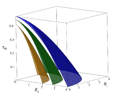
The nonclassical intensity depth has been determined for the experimental multimode twin beams in Ref. PerinaJr2013a ,
| (39) |
where
| (40) |
The analysis of Eq. (39) shows that the experimental multimode twin beam is strongly nonclassical () provided that
| (41) |
Inequality (41) means that the multimode strong nonclassicality of the twin beam is lost if the noise is sufficiently strong. For example, if , strongly nonclassical multimode twin beams are observed for (see Fig. 11). This behavior is similar to that discussed in Sec. IV, though the boundary given by is quantitatively different (compare Figs. 6 and 11). We also have here that the greater the value of the mean photon-pair number , the greater the value of the nonclassical intensity depth . Also, the greater the values of mean noise photon numbers and , the smaller the value of the nonclassical intensity depth .
Similarly as in Sec. VI, the logarithmic participation ratio can be defined for each component of the twin beam to quantify its dimensionality. The logarithmic participation ratio of the whole twin beam is then naturally given as the sum of the logarithmic participation ratio of the paired component and the logarithmic participation ratio of the noise signal and idler components. We note that Eq. (25) is appropriate for determining the participation ratio of both the single-mode noise signal (or idler) field and the single-mode paired field. Alternatively we may consider entropies of the components instead of participation ratios. Entropies of the single-mode noise fields are given by Eq. (33). Equation (33) is applicable also for determination of the entropy of entanglement of a single-mode paired field in a pure state for which . As a consequence, the entropies for , of each component are increasing functions of the corresponding participation ratios . In single-mode cases, these functions are determined by Eq. (35), plotted in Fig. 10. Similarly to the overall logarithmic participation ratio , the overall entropy can be naturally split into its entangled part and noisy part , originating in the noise signal and idler components.
Finally, we briefly address the issue of the experimental determination of the quantities discussed above. As these quantities characterize the “internal” structure of a twin beam, only their indirect determination is possible. It is based upon the measurement of the joint signal-idler photocount histogram using photon-number-resolving detectors. Knowing these detector parameters PerinaJr2012 , reconstruction of the joint signal-idler photon-number distribution PerinaJr2012a ; PerinaJr2013a provides the applied mean photon(-pair) numbers and numbers of modes. The above-derived formulas then give the discussed quantities.
VIII Conclusions
The entanglement and nonclassicality of a single-mode noisy twin beam have been quantified using the negativity and the nonclassical depth, respectively. Universal mapping between the nonclassical depth and the negativity has been revealed for noisy twin beams. The mapping reflects the fact that nonclassicality of a twin beam is caused by the entanglement of its two parts originating in pairing of photons. Limitations to the amount of noise have been found to preserve entanglement together with nonclassicality. the degrees of freedom of a twin beam quantified by the signal- and idler-field participation numbers have been divided into those needed to describe entanglement and the remaining ones forming the noisy signal and idler parts of the twin beam. The entanglement dimensionality derived from the negativity has been applied here. Entropy as an increasing function of the participation number has been discussed. Properties of multimode twin beams have been analyzed using appropriate quantities related per one mode. Also, experimental multimode twin beams containing additional noise in independent spatiotemporal modes have been investigated from the point of view of their entanglement and multimode nonclassicality including weak nonclassicality and dimensionality.
Acknowledgements.
I.A. and J.P. Jr. thank M. Bondani for discussions. Support by project LO1305 of the Ministry of Education, Youth and Sports of the Czech Republic is acknowledged. I.A. thanks project IGA_PrF_2015004 of IGA UP Olomouc. J.P. Jr. acknowledges project P205/12/0382 of GA ČR. A.M. was supported by the Polish National Science Centre under Grants No. DEC-2011/03/B/ST2/01903 and No. DEC-2011/02/A/ST2/00305.References
- (1) A. Einstein, Ann. Phys. 17, 132 (1905).
- (2) A. Einstein, B. Podolsky, and N. Rosen, Phys. Rev. 47, 777 (1935).
- (3) E. Schrödinger, Naturwissenschaften 23, 807 (1935).
- (4) J. Peřina, Z. Hradil, and B. Jurčo, Quantum Optics and Fundamentals of Physics (Kluwer, Dordrecht, 1994).
- (5) M. A. Nielsen and I. L. Chuang, Quantum Computation and Quantum Information (Cambridge University Press, Cambridge, 2000).
- (6) A. Migdall, Physics Today 52, 41 (1999).
- (7) V. Giovannetti, S. Lloyd, and L. Maccone, Nat. Photon. 5, 222 (2011).
- (8) J. Peřina Jr., O. Haderka, M. Hamar, and V. Michálek, Opt. Lett. 37, 2475 (2012a).
- (9) H. Vahlbruch, A. Khailaidovski, N. Lastzka, C. Graef, K. Danzmann, and R. Schnabel, Class. Quantum Grav. 27, 084027 (2010).
- (10) L. Mandel and E. Wolf, Optical Coherence and Quantum Optics (Cambridge University Press, Cambridge, 1995).
- (11) J. Peřina, Quantum Statistics of Linear and Nonlinear Optical Phenomena (Kluwer, Dordrecht, 1991).
- (12) D. F. Walls and G. J. Milburn, Quantum Optics (Springer, Berlin, 1994).
- (13) D. Bouwmeester, J. W. Pan, K. Mattle, M. Eibl, H. Weinfurter, and A. Zeilinger, Nature (London) 390, 575 (1997).
- (14) G. Weihs, T. Jennewein, C. Simon, H. Weinfurter, and A. Zeilinger, Phys. Rev. Lett. 81, 5039 (1998).
- (15) A. Lukš, V. Peřinová, and J. Peřina, Opt. Commun. 67, 149 (1988).
- (16) C. T. Lee, Phys. Rev. A 42, 1608 (1990a).
- (17) A. I. Lvovsky and M. G. Raymer, Rev. Mod. Phys. 81, 299 (2009).
- (18) O. Jedrkiewicz, Y. K. Jiang, E. Brambilla, A. Gatti, M. Bache, L. A. Lugiato, and P. Di Trapani, Phys. Rev. Lett. 93, 243601 (2004).
- (19) M. Bondani, A. Allevi, G. Zambra, M. G. A. Paris, and A. Andreoni, Phys. Rev. A 76, 013833 (2007).
- (20) J. Peřina Jr., O. Haderka, and V. Michálek, Opt. Express 21, 19387 (2013a).
- (21) M. Lamperti, A. Allevi, M. Bondani, R. Machulka, V. Michálek, O. Haderka, and J. Peřina Jr., J. Opt. Soc. Am. B 31, 20 (2014a).
- (22) M. Lamperti, A. Allevi, M. Bondani, R. Machulka, V. Michálek, O. Haderka, and J. Peřina Jr., Int. J. Quant. Inf. 31, 1461017 (2014b).
- (23) R. J. Glauber, Phys. Rev. 131, 2766 (1963).
- (24) E. C. G. Sudarshan, Phys. Rev. Lett. 10, 277 (1963).
- (25) V. Dodonov and V. Manko, Theory of Nonclassical States of Light (Taylor & Francis, New York, 2003).
- (26) W. Vogel and D. Welsch, Quantum Optics (Wiley-VCH, Weinheim, 2006).
- (27) T. Richter and W. Vogel, Phys. Rev. Lett. 89, 283601 (2002).
- (28) A. Miranowicz, M. Bartkowiak, X. Wang, Y.-X. Liu, and F. Nori, Phys. Rev. A 82, 013824 (2010).
- (29) M. Bartkowiak, A. Miranowicz, X. Wang, Y.X. Liu, W. Leoński, and F. Nori, Phys. Rev. A 83, 053814 (2011).
- (30) A. Allevi, M. Lamperti, M. Bondani, J. Peřina Jr., V. Michálek, O. Haderka, and R. Machulka, Phys. Rev. A 88, 063807 (2013).
- (31) W. Vogel, Phys. Rev. Lett. 100, 013605 (2008).
- (32) O. Haderka, J. Peřina Jr., M. Hamar, and J. Peřina, Phys. Rev. A 71, 033815 (2005).
- (33) J. Peřina Jr., M. Hamar, V. Michálek, and O. Haderka, Phys. Rev. A 85, 023816 (2012b).
- (34) J. Peřina Jr., O. Haderka, V. Michálek, and M. Hamar, Phys. Rev. A 87, 022108 (2013b).
- (35) C. T. Lee, Phys. Rev. A 41, 1721 (1990b).
- (36) A. Verma and A. Pathak, Phys. Lett. A 374, 1009 (2010).
- (37) R. Horodecki, P. Horodecki, M. Horodecki, and K. Horodecki, Rev. Mod. Phys. 81, 865 (2009).
- (38) A. Peres, Phys. Rev. Lett. 77, 1413 (1996).
- (39) P. Horodecki, Phys. Lett. A 232, 333 (1997).
- (40) K. Życzkowski, P. Horodecki, A. Sanpera, and M. Lewenstein, Phys. Rev. A 58, 883 (1998).
- (41) G. Vidal and R. F. Werner, Phys. Rev. A 65, 032314 (2002).
- (42) J. F. Clauser, M. A. Horne, A. Shimony, and K. A. Holt, Phys. Rev. Lett. 23, 880 (1969).
- (43) E.V. Shchukin and W. Vogel, Phys. Rev. Lett. 95, 230502 (2005); A. Miranowicz and M. Piani, Phys. Rev. Lett. 97, 058901 (2006).
- (44) A. Miranowicz, M. Piani, P. Horodecki, and R. Horodecki, Phys. Rev. A80, 052303 (2009).
- (45) C. T. Lee, Phys. Rev. A 44, R2775 (1991).
- (46) I. P. Degiovanni, M. Bondani, E. Puddu, A. Andreoni, and M. G. A. Paris, Phys. Rev. A 76, 062309 (2007).
- (47) M. Bondani, E. Puddu, I. P. Degiovanni, and A. Andreoni, J. Opt. Soc. Am. B 25, 1203 (2008).
- (48) I. P. Degiovanni, M. Genovese, V. Schettini, M. Bondani, A. Andreoni, and M. G. A. Paris, Phys. Rev. A 79, 063836 (2009).
- (49) C. Eltschka and J. Siewert, Phys. Rev. Lett. 111, 100503 (2013).
- (50) K. Życzkowski, Phys. Rev. A 60, 3496 (1999).
- (51) M. V. Fedorov, M. A. Efremov, A. E. Kazakov, K. W. Chan, C. K. Law, and J. H. Eberly, Phys. Rev. A 69, 052117 (2004).
- (52) M. V. Fedorov, M. A. Efremov, P. A. Volkov, E. V. Moreva, S. S. Straupe, and S. P. Kulik, Phys. Rev. Lett. 99, 063901 (2007).
- (53) K. W. Chan, J. P. Torres, and J. H. Eberly, Phys. Rev. A 75, 050101 (2007).
- (54) H. Di Lorenzo Pires, C. H. Monken, and M. P. van Exter, Phys. Rev. A 80, 022307 (2009).
- (55) K. Bartkiewicz, K. Lemr, and A. Miranowicz, Phys. Rev. A 88, 052104 (2013).
- (56) F. Just, A. Cavanna, M. V. Chekhova, and G. Leuchs, New J. Phys. 15, 083015 (2013).
- (57) K. Bartkiewicz, J. Beran, K. Lemr, M. Norek, and A. Miranowicz, Phys. Rev. A91, 022323 (2015).
- (58) K. Bartkiewicz, P. Horodecki, K. Lemr, A. Miranowicz, and K. Zyczkowski, Phys. Rev. A91, 032315 (2015).
- (59) J. Peřina and J. Křepelka, J. Opt. B: Quantum Semiclass. Opt. 7, 246 (2005).
- (60) A. Lukš, J. Peřina Jr., W. Leoński, and V. Peřinová, Phys. Rev. A 85, 012321 (2012).
- (61) V. Peřinová, A. Lukš, J. Křepelka, and J. Peřina Jr., Phys. Rev. A 90, 033428 (2014).
- (62) J. Peřina and J. Křepelka, Opt. Commun. 284, 4941 (2011).
- (63) C. K. Law and J. H. Eberly, Phys. Rev. Lett. 92, 127903 (2004).
- (64) A. Gatti, T. Corti, E Brambilla, and D. B. Horoshko, Phys. Rev. A 86, 053803 (2012).
- (65) M. V. Chekhova, G.Leuchs and M. Zukowski, Opt. Comm. 337, 27 (2015).
- (66) D. B. Horoshko, G. Patera, A. Gatti, and M. I. Kolobov, Eur. Phys. J. D 66, 239 (2012).
- (67) A. M. Peréz, T. S. Iskhakov, P. Sharapova, S. Lemieux, V. Tikhonova, M. V. Chekhova, and G. Leuchs, Opt. Lett. 39, 2403 (2014).
- (68) Arvind, N. Mukunda and R. Simon, Phys. Rev. A 56, 5042 (1997).
- (69) Arvind, N. Mukunda and R. Simon, J. Phys. A: Math. Gen. 31, 565 (1998).