The Galactic ²⁶Al emission map as revealed by INTEGRAL SPI

Abstract

Diffuse emission is often challenging since it is undetectable by most instruments, which are generally dedicated to point-source studies. The ²⁶Al emission is a good illustration: the only available ²⁶Al map to date has been released, more than fifteen years ago, thanks to the COMPTEL instrument. However, at the present time, the SPI spectrometer aboard the INTEGRAL mission offers a unique opportunity to enrich this first result. In this paper, $2\times 10^{8}$ s of data accumulated between 2003 and 2013 are used to perform a dedicated analysis, aiming to deeply investigate the spatial morphology of the ²⁶Al emission. The data are first compared with several sky maps based on observations at various wavelengths to model the ²⁶Al distribution throughout the Galaxy. For most of the distribution models, the inner Galaxy flux is compatible with a value of 3.3$\times$ 10^-4 ph cm^-2 s^-1 while the preferred template maps correspond to young stellar components such as core-collapse supernovae, Wolf-Rayet and massive AGB stars. To get more details about this emission, an image reconstruction is performed using an algorithm based on the maximum-entropy method. In addition to the inner Galaxy emission, several excesses suggest that some sites of emission are linked to the spiral arms structure. Lastly, an estimation of the ⁶⁰Fe line flux, assuming a spatial distribution similar to ²⁶Al line emission, results in a ⁶⁰Fe to ²⁶Al ratio around 0.14, which agrees with the most recent studies and with the SN explosion model predictions.

1. Introduction

The 1.809 MeV line emission associated with the ²⁶Al decay is one of the most intense gamma-ray lines observed in our Galaxy. It was first detected by the Ge spectrometer on the HEAO-C spacecraft (Mahoney et al., 1984). However, to date, only the COMPTEL Compton telescope aboard the Compton Gamma Ray Observatory has mapped the ²⁶Al during its nine years survey. The emission has been found mainly distributed along the Galactic plane and supports a massive-stars origin (Diehl et al., 1995; Oberlack et al., 1997; Knödlseder et al., 1999a; Plüschke et al., 2001). In addition, the early COMPTEL skymaps suggest a number of marginally significant spots, some of them being potentially associated with the Galactic spiral arms structure (Chen et al., 1996). However, most of these features remain compatible with statistical noise in the data (Knödlseder et al., 1999b).
These COMPTEL  maps have been used as a basis to fix the spatial morphology of the ²⁶Al line emission for subsequent works related to the spectral analyzes. Among them, detailed studies in the inner Galaxy and extended regions along the Galactic plane made with INTEGRAL SPI  indicate that the intrinsic line width is less than 1.3 keV and that line position shifts along the plane corresponding to the rotation of our Galaxy, confirming at least a partial association of the ²⁶Al emission with the spiral arms (Diehl et al., 2006; Wang et al., 2009; Kretschmer et al., 2013, and references therein).
A related topic is the ⁶⁰Fe emission, more precisely the isotope lines at 1.173 and 1.333 MeV released when it decays into ⁶⁰Co and ⁶⁰Ni, for the final stage of massive star evolution. Because of its weakness, the ⁶⁰Fe radiation has been detected from our Galaxy with only two instruments, RHESSI (Smith, 2004) and SPI  (Harris et al., 2005; Wang et al., 2007). The ⁶⁰Fe to ²⁶Al flux ratio is found to be about 0.15 by both instruments.
In this paper, 10 years of INTEGRAL observation are used to examine the spatial morphology of the ²⁶Al line, through direct sky-imaging and sky distribution model comparison. We will emphasize on the data analysis, especially the instrumental background modeling issue, a key point for both COMPTEL and SPI instruments. We have developed several methods, and try to derive reliable conclusions, independent of any specific (sky or background) model.
In the following sections, we review the main characteristics of the instrument and data-set and discuss the basic principles of the developed methods in Section 2. We then present the results (Section  3) on the global morphology of the ²⁶Al line emission, but also on specific regions suspected to harbor ²⁶Al progenitors, before discussing the outcomes in Section 4.

2. Data and analysis method

2.1. Instrument and observations

The International Gamma-Ray Astrophysics Laboratory (INTEGRAL) observatory was launched from Baïkonour, Kazakhstan, on 2002 October 17.
The on-board SPI spectrometer is equipped with an imaging system sensitive both to point-sources and extended/diffuse emission. It consists of a coded mask associated with a 19 Ge detector camera. This leads to a spatial resolution of $\sim$2.6^∘ over a field-of-view of 30^∘ (Vedrenne et al., 2003). The instrument’s in-flight performance is described in Roques et al. (2003). Due to its non-conventional coded mask imaging system, the imaging capability relies also on a specific observational strategy based on a dithering procedure (Jensen et al., 2003), where the direction of pointing of each exposure is shifted from the previous one by $\sim$2.2^∘. A revolution lasts 3 days, the time that the spacecraft performs a large eccentric orbit, but half of a day of data is unusable because of the radiation belts crossing. It contains generally about 100 exposures lasting approximately 45 minutes each.
The present analysis is based on public data recorded with the SPI instrument from revolution 44 (2003 February 23) to revolution 1287 (2013 April 28). Around 1 MeV, high-energy particles saturate the electronics and can generate false triggers. Nonetheless, it is possible to analyze the signal in this energy range thanks to another electronic chain (via Pulse Shape Discriminators or PSDs) not affected by the saturation problem. The procedure is explained in Jourdain & Roques (2009). We use the events which trigger only one detector (single-events). Note that the events which hit successively two or more detectors (multiple-events, representing $\sim$25$\%$ of the photons in this energy band) are not used in this work. After excluding data contaminated by solar flares or the radiation belts, it results in about 77 000 exposures and 2$\times$10⁸ s observation livetime.
We performed our analyzes of the ²⁶Al line emission in the 1805-1813 keV band, to take into account the Germanium energy resolution (FWHM of 2.9 keV at 1764 keV), including its degradation between two consecutive annealings ($\sim 5\%$). At these energies, the gain calibration (performed orbit-wise) accuracy is better than $\pm$0.01 keV.

2.2. Data modeling

The signal recorded by the SPI camera on the 19 Ge detectors is composed of contributions from each source (point-like or extended) present in the field-of-view, convolved by the instrument aperture, plus the background. For extended/diffuse sources, we assume that their spatial distributions are given by an analytical function or an emission map (Section 2.3) whose intensities are to be determined. For a given energy band and for $N_{s}$ sources located in the field of view, the data $n_{dp}$ obtained during an exposure (pointing) p for the detector d can be expressed by the relation:

$$n_{dp}=\sum_{j=1}^{N_{s}}R_{dp,j}s_{j}+b_{dp}+\epsilon_{dp}$$ (1)

where $s_{j}$ is the intensity of source j. $R_{dp,j}$ is the response of the instrument to source j, $b_{dp}$ the background, and $\epsilon_{dp}$ the statistical noise (both for exposure p and detector d). We assumed that there are $N_{p}$ exposures and $N_{d}$ detectors.
At the energies considered in this paper (E $>$ 1 MeV), point-source emissions are weak and stable in time within the measurement uncertainties. Concerning the extended/diffuse sources, they are not expected to vary. Thus, for a given set of $N_{p}$ exposures and $N_{d}$ detectors, the system of equations, as formulated above, requires $N_{p}\times N_{d}$ equations to solve for $N_{s}+N_{p}\times N_{d}$ unknowns. Hence, it is mandatory to reduce the number of unknowns. We will see below that the observed properties of the background allow us to strongly decrease the corresponding number of free parameters. Finally, to determine the sky model parameters, we adjust the data through a multi-component fitting algorithm, based on the maximum likelihood statistics. Expected counts are obtained by convolving a sky model with the instrument response and then adding the background model. The resulting distribution is compared to the recorded data with free normalizations of both components. We used Poisson’s statistics to evaluate the adequacy of the various sky models to the data. The core algorithm developed to handle such a large system is described in Bouchet et al. (2013a).

2.3. Modeling of the ²⁶Al spatial distribution

A way to estimate the ²⁶Al emission spatial distribution over the Galaxy (i.e. the corresponding $s_{j}$ term in Equation 1) is to represent it with some templates. In this study, we have used maps listed in Table 1, similarly to Knödlseder et al. (1999a) for the COMPTEL data. These maps, although the list is not exhaustive, emphasize some large-scale structures of the sky observed at particular wavelengths and associated to specific emission mechanisms that we may relate to the ²⁶Al emission.
Specific treatments have been applied to some of them: The A[${3.5\mu}$] and A[${4.9\mu}$] maps are the NIR 3.5 and 4.9$\mu$ maps corrected for reddening using NIR 1.25$\mu$ map and averaging emission at latitude $|b|>40^{\circ}$ to estimate the zero level emission as explained in Krivonos et al. (2007, and references therein). Note that, with this procedure, the extra-galactic component has been removed, but the resulting maps are not expected to have an accuracy better than $\sim 10\%$. For the CO (Dame, Hartmann & Thaddeus, 2001) and the EGRET ($>$ 100 MeV) (provided by the NASA/Goddard Space Flight Center) maps, we apply the pre-treatment detailed in Knödlseder et al. (1999a, and references therein). Hence, the peak emission around the Galactic Center of the CO map has been removed, while point-sources from the second EGRET catalog have been subtracted from the EGRET map, together with an isotropic intensity of 1.5$\times$ 10^-5 ph cm^-2 s^-1 sr^-1 to take into account the cosmic diffuse background radiation.
We have introduced a parameter to quantify the difference between all these maps, the contrast, which we defined as the ratio of the flux contained in the region $|l|\leq 150^{\circ}$, $|b|\leq 15^{\circ}$ to the total flux enclosed in $|l|\leq 180^{\circ}$, $|b|\leq 90^{\circ}$. This ratio varies from 0.4, for the 25$\mu$ MIR map, to almost 1, for the A[${4.9\mu}$] map. For reference, the EGRET map, which traces the interstellar gas/cosmic-ray emission, has a contrast value of 0.7. The maps up to EGRET (left part of the x-axis of Figures 6 and 7) are said to have low-contrast and those above (right part) high-contrast.

2.4. Background determination

The instrumental background corresponds to a more or less isotropic component due to particles hitting the telescope or created inside its structure. It is the main contributor to the flux recorded by the detector plane and represents a key issue since the signal-to-noise ratios considered in this study are below 1$\%$.
However, we have to note that the background term in Equation (1), formally consisting of $M=N_{d}\times N_{p}$ values (one per detector and per pointing), can be rewritten as:

$$b_{dp}=a_{p}\times u_{d}\times t_{dp}$$ (2)

Here $u$ is a vector of $N_{d}$ elements, representing the ”uniformity map” of the detector plane (background pattern), $t_{dp}$ the effective observation time for detector d and pointing p. The evolution of the background intensity is traced with $a_{p}$, a scalar normalization coefficient per pointing. Assuming that $u$ is determined elsewhere, the number of unknowns (free parameters) in the set of $N_{p}\times N_{d}$ equations is reduced to $N_{s}+N_{p}$ (for a background intensity varying on the exposure timescale). However, the background intensity ($a_{p}$) does not necessarily vary so rapidly and the number of related background parameters could be still decreased, according to the actual background evolution.
We detail below both aspects (detector pattern and timescale evolution) of the background determination.

2.4.1 Background intensity variations

Figure 1 shows the mean count rate (per detector) evolution with time. In our standard analysis, we generally assume that the background varies with a fixed timescale. We have tested several timescales from one exposure ($\sim$ 2-3 ks) to one revolution ($\sim$ 2-3 days) and compared the results from a statistical point of view. Figure 2 shows the evolution of several indicators as a function of the chosen timescale. The ”reduced chi-square” is defined as $\chi^{2}_{L}/dof$, where $\chi^{2}_{L}$ stands for the likelihood equivalent chi-square and $dof$ for the degrees of freedom.
The reduced chi-square (or similarly $\chi^{2}_{L}-dof$) is rather stable for timescales less than 12 hours; above, its value increases very quickly. As we aim to have as few as possible free parameters, in order to get a better conditioned system of equations, we can consider that a timescale of $\sim$ 9 hours is a reasonable trade-off. In comparison, for the 505-516 keV band, we have concluded in Bouchet et al. (2010) that the best quality and robust results are obtained with a value of $\sim$ 6 hours. Note that the behavior of the above quantities does not depend on the assumed synthetic map nor on the pattern determination method (Section 2.4.2).
However, to impose segments of fixed duration is convenient and easy, but not necessarily the best way to proceed since the background intensity can vary with various timescales along the mission. We have therefore applied a segmentation algorithm developed to determine the variability timescale of the sources (Bouchet et al., 2013b) to the background signal. We first subtracted the source contribution from the total counts. A rough approximation of the sky signal is enough for this purpose (its contribution to the total counts is weak). Then, for each exposure, counts are summed over all detectors, and for each revolution, the corresponding time-series (up to one hundred of exposures) is segmented. The number of segments and their lengths are adjusted in order to obtain the minimal number of segments ensuring $\chi^{2}$/dof $\leq$ 1. Figure 3 illustrates the case where the background intensity varies with different timescales along the revolution.
The background intensity has been found stable (fit with one segment) during 477 over 1081 revolutions. Finally, the total number of segments has been significantly reduced since only $\sim$3000 segments are required to describe the whole dataset, instead of the $\sim$12 000 segments used when fixing a $\sim$6 hours timescale. To compare qualitatively these results with those obtained with fixed timescales, we plot in Figure 2 the statistical quantities corresponding to the background segmentation method with isolated symbols (arbitrary abscissa since no fixed timescale). All of them point toward an improvement of the fit quality when the background variability is determined with a flexible timescale. Finally, these (quasi model-independent) time segments have been used to describe the background evolution in our subsequent analyzes.

2.4.2 ”Uniformity map”

The uniformity map or background pattern ($u$ in Equation 2) can be fixed by hand before the fitting procedure by using “empty-field” observations, thought to contain no source signal. The dedicated SPI  “empty-field” observations are rare, but the exposures whose pointing latitude direction satisfies $|b|>30^{\circ}$ constitute a good approximation since they contain only weak contributions from sources, at the energies considered here. They amount to 20$\%$ of the observations and have been used for building a set of background templates for different periods along the mission (about one per 6 months).
To quantify the properties of the background pattern for each period, we define the vector $u$ as

$$u(d)=\frac{\sum_{p}d_{p}(d)}{\sum_{p}t_{p}(d)}~{}\mathrm{for~{}exposure~{}p~{}satisfying~{}|b|\geq 30^{\circ}}$$ (3)

However, in the case of diffuse emission, the high-latitude exposure fields may contain some signal and the background pattern deduced from them may be ”blurred”. More precisely, the high-latitude $|b|>30^{\circ}$ regions contain $\sim$ 30$\%$ to 40$\%$ of the total emission for the ”low-contrast” maps (12$\mu$, 25$\mu$ and synchrotron) while this ratio is less than 10$\%$ for ”high-contrast” (EGRET to A[${4.9\mu}$] maps) ones. Consequently, if the true emission distribution approaches the 25$\mu$ map, the detector pattern will be more affected by the high-latitude emission than if the true emission distribution follows the A[${4.9\mu}$] map. Note that the effect on the measured source flux is not predictable since the fit procedure adjusts background and source normalizations: a “bad” background pattern may imply an underestimation or an overestimation of the source flux.
In addition, for the ²⁶Al study, we have to keep in mind that the side shields do not stop 100% of photons. This means that any uniformity map or background pattern will contain also some diffuse emission signal passing through the shield.
We have investigated another approach to estimate the detector uniformity pattern, by fitting it during the convergence procedure. We have to note, in this case, that a prerequisite is to have a sufficient knowledge of the source contribution and that the background model relies on more free parameters. With this alternative method, the $\chi^{2}_{L}$ decreases by $\Delta\chi^{2}_{L}\sim$8200 for $\Delta$dof=411 additional parameters (2973 parameters are used to describe the background). However, the improvement of the $\chi^{2}_{L}$ criterion is not reliable enough since the recovered source signal becomes background dependent and can be altered to an extent which is difficult to estimate.
The two pattern determination methods are subsequently referred to as fixed-pattern and fitted-pattern ones, and we have systematically compared the results obtained with each of them.

Figure 4 presents the ²⁶Al line flux obtained in the inner Galaxy ($|l|\leq 30^{\circ}$, $|b|\leq 10^{\circ}$) for both pattern determination methods and several background variability timescales with the same model for the ²⁶Al distribution (here the 60$\mu$ template). With the fixed-pattern method, the recovered flux depends on the assumed background timescale, especially for background timescales below 6 hours, while its value remains unaffected when the background pattern is adjusted. It is worth noting that the same analysis has been applied to the annihilation radiation, at 511 keV. Due to a better statistic and possibly a relatively less emission at high-latitudes, the fluxes obtained with the two pattern determination methods are perfectly compatible for each of the sky components, whatever the assumed background variation time-scales.

2.5. Imaging the sky

Although the model-fitting process provides the best quantitative information about the global emission and is better suited to determine its level of confidence, a direct “imaging” algorithm provides more qualitative information such as the position of potential emitting sources and their extent as well as some basic, but model independent, characteristics of the emission morphology.
To build an image, the sky is divided into small areas or pixels, the flux $f$ in each pixel is to be determined. The linear model of the data derived from Equation (1) is put in a more synthetic form through

$$n=Rf+b+\epsilon$$ (4)

where $n$ represents the data, $b$ the background, $R$ the response of the instrument as described in Section 2.2 and $\epsilon$ the statistical noise. $n$, $b$ and $\epsilon$ are vectors of length $M$ (the number of data points), $f$ a vector of length $N$ (the number of pixels in the sky) and $R$ a matrix of size $M$ by $N$. The statistical noise is assumed to follow a Gaussian distribution with a variance $\sigma^{2}$ and null mean.
However, when the number of pixels is large, the system of equations becomes ill-conditioned; the direct least-square solution is not always reliable and generally poorly informative. To select an informative and particular solution, the most common technique consists in including a regularization term in the above system, in addition to the least square constraint. This solution, although biased by the choice of the regularization criterion, improves the conditioning of the system. A compromise between the goodness of the fit, quantified by $\chi^{2}$, and the regularization, say $H$, is found by maximizing the function

$$Q(f)=\alpha H(f)-\frac{1}{2}\chi^{2}(f)$$ (5)

where $\alpha$ is a parameter, which determines the degree of smoothing of the solution.
We choose to use one of the most popular regularization operators: the entropy function. This method is known as the Maximum-Entropy Method or MEM (Gull, 1989, and references therein). For an assumed positive additive distributions,

$$H(f)=\sum_{i=1}^{N}f_{i}-m_{i}-f_{i}log\frac{f_{i}}{m_{i}}$$ (6)

where $m_{i}$ is the default initial value assigned to the pixel $i$. Note that $f_{i}$ and $m_{i}$ are positive quantities. MEM has been proved to be a successful technique for astronomical image reconstruction (Skilling, 1981). The algorithm is described in Apppendix A. However, despite its capabilities, it suffers from several shortcomings: among them, the difficulty of selecting the appropriate entropy function distribution and the default pixel values. In addition, the possible correlations between pixels are not taken into account properly. One way to remedy this problem is described in Section 2.5.2.

2.5.1 Including the background intensity determination

In our application, the instrumental background could be fixed through the modeling method presented in Section 2.4. However, such a modeling, even though being accurate enough for the model-fitting procedure, may be a source of biases for the image reconstruction, by preventing the appearance or by exaggerating the significance of some structures potentially present in the image. Consequently, we prefer to have the possibility to refine the parameters linked to the background intensity during the image reconstruction process. The instrumental background variation timescale is fixed through the modeling method presented in Section 2.4. We search for both the solution vector $f$ (length $N$) and the background intensities, $b$ (length $N_{b}$). We assume that the background parameters are precisely determined/constrained (small error bars) compared to sky pixels, hence they do not require any smoothing. Note that the ”cross-talk” effects between sky pixels and background parameters are reduced since the number of parameters to describe the background is nearly minimum (Section 2.4.1).

2.5.2 Pixel correlation

As mentioned above, the possible correlations between the pixels of the image (the sky emission should vary smoothly from one pixel to the next ones) are not taken into account properly with the entropy function. It is possible to introduce artificially such a correlation by using an Intrinsic Correlation Function, ICF, (Gull, 1989). The function to maximize becomes:

$$Q(f)=\alpha H(f)-\frac{1}{2}\chi^{2}(f_{ICF})~{}\mathrm{where}~{}f_{ICF}\equiv ICF(f)$$ (7)

For our work, we choose a radial Gaussian function. Such an ICF takes part largely to the solution regularization by ensuring its smoothness.

2.5.3 Construction of a sky image

In practice, the sky is divided into pixels of equal area, following the Healpix (Hierarchical Equal Area isoLatitude Pixelization of a sphere) scheme (Gorski et al., 2005), and initialized with a uniform default value. In a first step, we consider a very low-resolution map (48 pixels of $\sim 29^{\circ}$ resolution) and select the value of $\alpha$ such that the reconstructed flux in the inner Galaxy is comparable to the value obtained with the model-fitting procedure. The size of this problem is relatively small and a N-dimensional search-algorithm is used to maximize the function $Q$ ($\sim$3000 parameters). The calculation of the first-order solution (image and background parameters) is based on a classical Newton type optimization algorithm with a positivity constraint on the solution. During this first stage, the background pattern is fixed. The resulting image is used as a template to compute an improved pattern which is then fixed for the rest of the process. We then use this solution as a starting point (for an initial guess of the background parameters, the image is assumed to be flat) to build a high-resolution image (49 152 pixels of 0.9^∘ resolution) through an algorithm similar to that proposed by Skilling & Bryan (1984). The parameter $\alpha$ and the uniform sky default model are computed at each iteration so that the solution is ensured to follow the optimum MEM trajectory (See Appendix A). At the end, the final solution satisfies $\chi^{2}/dof\simeq 1$ and fulfills an additional test on the degree of non-parallelism between the gradient of $C$ and $H$ (see Appendix A). Note that, the greater the number of iterations is, the lower the chi-square value but the image is more “spiky”. The above mentioned stopping criteria results probably in a ”spiky”, but also more objective image (Skilling & Bryan, 1984).

3. Results

3.1. Imaging

The image displayed in Figure 5 indicates that the emission is essentially confined in the inner Galaxy region ($|l|\leq 30^{\circ}$, $|b|\leq 10^{\circ}$), with a flux in the inner Galaxy of 3.5$\times 10^{-4}$ph cm^-2 s^-1 . Note that the morphology is drastically different from the electron-positron annihilation line emission one, which is essentially concentrated in the bulge region (Weidenspointner et al., 2008; Bouchet et al., 2010; Churazov et al., 2010).
Beyond the morphology of the diffuse emission, our interest has been piqued by several spots visible in the image. Simulations of image reconstruction (Appendix B) show that structures with a peak intensity at $\sim$one-tenth of the image maximum intensity are probably due to residual statistical noise. Above this level, structures are worth being considered carefully. Indeed, some of them have positions compatible with sources detected or studied during recent SPI investigations (See section 3.3). For instance, the image reveals several excesses in the Cygnus region (72${}^{\circ}<l<96^{\circ}$, -7${}^{\circ}<b<7^{\circ}$). A significant one is located at a position compatible with Cyg OB2 cluster (81^∘,-1^∘) as reported by Martin et al. (2009). In the Sco-Cen region (328${}^{\circ}<l<355^{\circ}$, 8${}^{\circ}<b<30^{\circ}$), the strongest excess is localized at (l, b) $\approx$(360^∘, 16^∘), having a spatial extent with a radius of 5^∘. Some structures appear also around the Carina and Vela regions and two others, more extended, in the Taurus/Anticenter region (105${}^{\circ}<l<170^{\circ}$, -15${}^{\circ}<b<20^{\circ}$). Finally, an additional spot detected above 3$\sigma$ is worth investigating. However, a model-fitting analysis is required to extract more quantitative information on the above mentioned structures (Section 3.3).

3.2. Testing template maps

This analysis is similar to that done with the COMPTEL data by Knödlseder et al. (1999a), and consists of using template maps to model the spatial distribution of the ²⁶Al emission through the Galaxy. In this case, only the intensity normalization is adjusted (1 parameter) in addition to the background parameters. In practice, we fit the data with a combination of one of the maps listed in Table 1 plus a background model. The template preparation is detailed in Section 2.3.
To qualify the detection significance of the ²⁶Al emission for a given template, we adjust two models to the data: the first one contains only the background while the second contains the background plus the tested template map. Quantitatively, the improvement of the likelihood is 512 for 1 additional parameter for the 25$\mu$ map (best model) and the background determined with the fixed-pattern method. The ²⁶Al flux detection significance is $\sim 23\sigma$, and the associated reduced-chi-square is $\chi^{2}_{L}/dof=1.0038$. Indeed, each template leads to a significant flux detection. The worse case, H_I map, has a significance of $\sim 17\sigma$.
The same analysis with the fitted-pattern background determination gives an improvement of the likelihood of 312 (for the 100$\mu$ map). The ²⁶Al flux detection significance is $\sim 18\sigma$ and $\chi^{2}_{L}/dof=0.9973$.
Figure 6 displays the Maximum Likelihood Ratio (MLR) obtained with both pattern determination methods (fixed and fitted-pattern) for each of the tested maps (ordered by increasing contrast). Several maps give similar results, leading to the conclusion that star-related distributions (FIR and MIR maps, dust and free-free distributions, all with rather high-contrast) give a good description of the data, as expected from what we know about the ²⁶Al emission process. Similarly, 25$\mu$ and 12$\mu$ maps constitute good tracers, while presenting a low-contrast. In another hand, H_I and 53 GHz synchrotron maps can be excluded. In fact, we have seen (Figure 5) that the emission is confined into the central part of the Galaxy and close to the disk. This explains why the H_I map does not provide a good fit to the data since it extends far in longitude and contains important emission at $|l|\geq 30^{\circ}$. We can also point out that distributions built by imaging method (MEM or MREM) from COMPTEL data appear as good tracers of the ²⁶Al emission, as expected.
As shown in Figure 7, the reconstructed flux attributed to the inner Galaxy does not depend much on the template map and is compatible with a value of $3.3\times$ 10^-4 ph cm^-2 s^-1 , in agreement with the previously reported values. We observe that the flux is systematically higher by $\sim$8 (low-contrast maps) to 20$\%$ (high-contrast maps) when the fixed-pattern background determination method is used, but it has no scientific implication. However, the total flux integrated over the whole sky clearly depends on the contrast of the assumed model. The more the map is contrasted (from left to right on Figure 7), the weaker is the reconstructed total flux. This is due to the fact that the recovered global intensity relies on the central parts of the image (both higher flux and signal to noise ratios) and that a contrasted map encompasses less flux in its external parts than a flatter map. Moreover, we are aware that low-contrast maps may suffer from significant “cross-talk” between the low-spatial frequency structure (a kind of pedestal which mimics a flat low-surface brightness emission) and the (more or less uniform) background contribution.
As an additional test, we have performed correlations between the direct image with 6^∘ resolution (e.g. ICF of 6^∘ FWHM) and each of the templates downgraded to the same $\sim$6^∘ spatial resolution (except the DMR/COBE 53 Ghz one, which originally has 7^∘ resolution). Indeed, the linear correlation coefficient does not depend much on the template map and keeps a value greater than 0.9 in latitude, and above 0.7 in longitude, except the H_I map (coefficient of 0.4 in longitude).
Finally, it appears that it is hard to firmly conclude about a unique solution. This reflects the difficulty of determining precisely such an extended weakly emitting structure and the similarity presented by most of the considered maps. However, we note that the $\chi^{2}$ curves follow the same evolution regardless the background determination method and hence that the conclusions do not depend on it.

3.3. Regions of potential excesses

To check quantitatively the significance of the most significant excesses and known ²⁶Al emitting regions, we have performed a more complete model-fitting analysis. Note, however, that our analysis is not optimized for extended point-sources since a map contribution is necessarily subtracted at the position of the sources and, at worse, may make them disappear.
The sky model consists of one of the templates listed in Table 1, to which is added a spatial model including the spots. For the sources already detected or investigated at 1.8 MeV, we have used the positions and spatial extensions provided by previous works (Vela (Diehl et al., 1995), Cygnus region (Martin et al., 2009), Sco-Cen (Diehl et al., 2010), Orion/Eridanus, (Voss et al., 2010) and Carina (Voss et al., 2012), indicated in bold in Table 1). To investigate the additional spots not yet referenced as ²⁶Al emitters, the extent and location are based on the image analysis using simple models (point-source, Gaussian or disk). However, given their low-significance and the SPI spatial resolution of 2.6 ^∘, their identification with known sources is just indicative. We report in Table 2, the flux values obtained using the IC (low-contrast) and A[${4.9\mu}$] (high-contrast) maps, as representative of the global results.
The Cyg OB2 cluster (81^∘,-1^∘) has a flux of ($4.1\pm 1.5$)$\times$ 10^-5 ph cm^-2 s^-1  similar to the value of ($3.9\pm 1.1$)$\times$ 10^-5 ph cm^-2 s^-1 obtained by Martin et al. (2009) and the ($3.7\pm 1.1$)$\times$ 10^-5 ph cm^-2 s^-1 obtained with COMPTEL (Plüschke et al., 2000). We note also another excess at (l,b)$\approx$(100^∘,6^∘) with a flux of (2.7 $\pm$ 1.1)$\times$ 10^-5 ph cm^-2 s^-1.
Strong emission has been reported in the Sco-Cen region by Diehl et al. (2010) centered around (l, b) = (350^∘, 20^∘). At this position, we find a flux ($4.1\pm 1.6$)$\times$ 10^-5 ph cm^-2 s^-1 when using an $H_{I}$ map to model the large scale ²⁶Al emission. However in our image, the local maximum in this region appears shifted to (l, b) $\approx$(360^∘, 16^∘), and the source is less extended (disk radius of 5^∘ instead of 10^∘ as reported by Diehl et al. (2010)), while the flux remains at ($4.1\pm 1.1$)$\times$ 10^-5 ph cm^-2 s^-1 using again the $H_{I}$ map. On the another hand, in both cases the flux clearly depends on the template map used and is less than 2$\sigma$ for most of the cases.
The Carina and Vela regions are marginally detected (2$\sigma$). For Carina, the measured flux of ($2.8\pm 1.5$)$\times$ 10^-5 ph cm^-2 s^-1 is comparable to the estimation of ($1.5\pm 1.0$)$\times$ 10^-5 ph cm^-2 s^-1 reported by Voss et al. (2012) using SPI data, and ($3.1\pm 0.8$)$\times$ 10^-5 ph cm^-2 s^-1 reported by Knödlseder et al. (1996) using COMPTEL data. For Vela, the flux of ($3.3\pm 1.8$)$\times$ 10^-5 ph cm^-2 s^-1 is comparable to the value ($3.6\pm 1.2$)$\times$ 10^-5 ph cm^-2 s^-1 reported by Diehl et al. (1995) using COMPTEL data. For the Orion-Eridanus area (180${}^{\circ}<l<210^{\circ}$, -30${}^{\circ}<b<5^{\circ}$), we get an upper limit for the total flux of 3$\times$ 10^-5 ph cm^-2 s^-1 (1 $\sigma$) in agreement with the value of (4.5 $\pm$ 2.1)$\times$ 10^-5 ph cm^-2 s^-1  obtained by Voss et al. (2010) from a synthesis model based on the Orion star populations. We also mention the the 2$\sigma$ upper limit of 1.7$\times$ 10^-5 ph cm^-2 s^-1 reported by Oberlack et al. (1995) for the Orion region using COMPTEL instrument.
Concerning the spots not yet reported, we first point out two extended structures in the Taurus/Anticenter region (105${}^{\circ}<l<170^{\circ}$, -15${}^{\circ}<b<20^{\circ}$) with fluxes of ($5\pm 2$) and ($8\pm 3$)$\times$ 10^-5 ph cm^-2 s^-1. Finally, a spot worth mentioning since it is detected above 3 $\sigma$, it is located at high-latitude (l,b)$\approx$(226^∘76^∘) with a flux of (7 $\pm$ 2)$\times$ 10^-5 ph cm^-2 s^-1. We did not find any convincing potential counterpart, but consider the stability of the attributed flux against the assumed ²⁶Al diffuse emission map as a good criterion to assess that an excess is robust and reliable.
We did not notice any systematic effect in the source flux determination between the fixed and fitted background pattern adjustment method. Note that adding all these excesses into the model of the sky improves the likelihood only marginally ($\Delta\chi^{2}_{L}\sim 5$) compared to the case where they are neglected, and that dedicated analyzes must be conducted to refine individually each result.

3.4. ⁶⁰Fe and ⁶⁰Fe to ²⁶Al ratio

While the intensity of the ⁶⁰Fe isotope emissions at 1.173 and 1.333 MeV contains important complementary information for the star evolution study, the weakness of the flux makes it impossible to derive any constraint on the spatial distribution. The latter is, therefore, assumed to be the same as the ²⁶Al line one (Section 3.2), which is physically reasonable since ²⁶Al and ⁶⁰Fe are believed to be produced at least partly in the same sites (e. g., massive stars and supernovae, Timmes et al. (1995), Limongi & Chieffi (2006)).
For this study, we followed basically the same procedure as for the ²⁶Al one. We analyzed the same dataset in the 1170-1176 and 1330-1336 keV bands, with the same templates to estimate the ⁶⁰Fe flux. The background determination method (Section 2.4.1) leads to the identification of 2900 and 2961 time-segments respectively. Note that the contribution of the ²⁶Al line through its interactions with the detectors (Compton effect, diffusion,…) has to be taken into account for the ⁶⁰Fe analysis. Being a strong line, ²⁶Al photons can interact inside the camera through the Compton effect and diffusion (the instrument response is non-diagonal) and produce a continuum from 20 keV to 1.8 MeV in the data-space. This emission component is thus convolved with the instrument response to predict the corresponding counts in the data-space, and the predicted counts in the 1170-1176 and the 1330-1336 keV bands are included in the sky model during the ⁶⁰Fe fluxes analysis. Moreover, the contribution from the diffuse continuum has been taken into account assuming the power law model determined in a previous work (Bouchet et al., 2011). Note that these effects are very small, well below the statistical error bars.
For all the tested distributions, the ⁶⁰Fe isotope lines are detected at a level of 2$\sigma$ and 3$\sigma$ respectively, in the 1170-1176 and 1330-1336 keV bands (Table 3). Their global mean-flux in the inner Galaxy is about 4$\times$ 10^-5 ph cm^-2 s^-1. Systematics in the flux determination of these large-scale structures due to the background pattern determination method is below $\sim$25$\%$ for the ²⁶Al and around $\sim$30$\%$ for the ⁶⁰Fe lines (fluxes obtained with the fixed-pattern are systematically higher).
As a conclusion, even though poorly constrained, the ⁶⁰Fe to ²⁶Al ratio obtained during this analysis is around 0.14 , which agrees with values previously obtained by Smith (2004) and Wang et al. (2007).

4. Discussion and Conclusion

For more than a decade, the reference map for the spatial morphology of the ²⁶Al emission was provided by COMPTEL. Several maps have been published, along the CGRO mission, with more and more data, but also different analysis methods. Consequently, while the extended morphology of the emission is assessed and results compatible, some local features not always appearing, depending on the method. Indeed, the first MEM images (Diehl et al., 1995; Oberlack et al., 1997) exhibit many low-intensity structures. A small number of them remain in the latest MEM image (Plüschke et al., 2001), giving some confidence in their reliability. In parallel, the chief features of these MEM images were confirmed with a MREM algorithm (Knödlseder et al., 1999b). This algorithm is based on an iterative expectation maximization scheme and a wavelet filtering algorithm. This wavelet filter suppresses the low-significance features, which are potential artifacts, by applying a user-adjustable threshold. This aims to produce the smoothest image consistent with the data (Knödlseder et al., 1999b). Note that the early MREM map built from SPI data by Knödlseder et al. (2006) was too rough to bring any additional information compared to COMPTEL ones.
Now that more than 10 years of SPI data are available, our main goal was to refine the COMPTEL view of the ²⁶Al line emission at 1.8 MeV and to investigate the related ⁶⁰Fe lines around 1.2 and 1.3 MeV. To study their spatial morphology, we have developed specific tools. We have performed two kinds of image reconstructions. The first one is based on existing maps, at various wavelengths, which are used as a sky model, convolved with the instrument response and compared to the data (model-fitting). The second one consists in direct sky reconstruction from the data, implying an inverse-problem. While the first method reveals the global large scale morphology of the emission, the latter allows us to look for small scale structures like local regions of ²⁶Al production.
The ²⁶Al line is detected at $\sim 20\sigma$, to compare to the $\sim 30\sigma$ obtained with the analysis of COMPTEL data obtained in 5 years (Knödlseder et al., 1999a).
In addition, comparing the MREM COMPTEL image (Knödlseder et al., 1999b) and SPI one, we report that a number of structures appear in both analyzes. Note that the SPI sky exposition is non-uniform, mostly concentrated along the Galactic plane and differs from the COMPTEL one. Thus, SPI is more sensitive in the Galactic plane than at high-latitudes, with a point-source (3 $\sigma$) sensitivity of 1.4$\times$ 10^-5 ph cm^-2 s^-1 in the Galactic Center region to be compared to the 0.8 to 1.4$\times$ 10^-5 ph cm^-2 s^-1 reported by Plüschke et al. (2001) for COMPTEL.

4.1. Data analysis : issues and solutions

A first point to mention is that, for SPI as for COMPTEL, the background treatment is a tricky issue. In SPI data, to disentangle the signal and the instrumental background contributions, we rely on the ability of the instrument to measure simultaneously both of them, due to the properties of the coded-mask aperture imaging system. Moreover, the evolution of the background intensity with time can be determined with a segmentation code developed specifically to take into account the background variation. The major advantage is that it strongly reduces the number of parameters related to the background. In a second step, we determine the background detector pattern by assuming that high-latitude exposures constitute a good approximation of “empty-fields”. However, they may contain signal from the diffuse emission (Section 2.4.2) We have thus implemented the possibility to determine the background pattern during the data-reduction process, assuming that the signal is sufficiently well known. The two approaches for background pattern determination have been compared to assess the robustness of the results, leading us to essentially the same conclusions regarding the ²⁶Al emission characteristics.

4.2. ²⁶Al and ⁶⁰Fe large-scale emission

In the model fitting analysis based on other wavelength maps, our data do not allow us to distinguish a unique preferred template since several ones lead to similar likelihood parameter values. From COMPTEL data, Knödlseder et al. (1999a) had concluded that the best tracers were DIRBE 240$\mu$ and 53 GHz free-free maps. We agree that the FIR maps with wavelengths 60 to 240 $\mu$ or 53 GHz (free-free and dust) appear statistically as the best estimates of the ²⁶Al emission global morphology but CO, NIR A[4.9$\mu$] and A[3.5$\mu$] extinction-corrected maps have also to be considered with only a slightly lesser degree of confidence. In addition, “low-contrast” maps observed at 25$\mu$ and 12$\mu$ provide an equally good description of the emission.
Indeed, our results confirm that the ²⁶Al emission follows more or less the distribution of the extreme Population $I$, the most massive stars in the Galaxy (Diehl et al., 1995). It is known that the massive stars, supernovae and novae produce the long-lived isotopes ²⁶Al and ⁶⁰Fe with half-lives of 0.7 and 2.6 My. On the another hand, large amounts of dust/grains condense in core collapse SNe ejecta while massive star-supernovae are major dust factories, therefore dust FIR and MIR maps are expected to correlate with the corresponding emissions.
Quantitatively, the flux extracted through the model fitting method for the inner Galaxy ($|l|\leq 30^{\circ}$,$|b|\leq 10^{\circ}$) is found to be around 3.3$\times$ 10^-4ph cm^-2 s^-1 while it does not depend much on the sky model (particularly if we restrict ourselves to the preferred ones). This flux is consistent with earlier measurements of both INTEGRAL SPI and COMPTEL instruments and corresponds to a total ²⁶Al mass contained in our Galaxy of $\sim$3$M\sun$,(but, see also Diehl et al. (2010) and Martin et al. (2009)). However, Churazov et al. (2010) using a ”light-bucket” method obtain a flux of 4 $\times$ 10^-4 ph cm^-2 s^-1 for the region delimited by $|l|\leq 40^{\circ}$,$|b|\leq 40^{\circ}$. For the same region, we obtain a flux of $\sim$ 3.9 $\times$ 10^-4ph cm^-2 s^-1 with the most probable spatial morphologies.
Another observable quantity, related to ²⁶Al production, is the ratio between ⁶⁰Fe and ²⁶Al line fluxes in the inner Galaxy. From a theoretical point of view, the ⁶⁰Fe to ²⁶Al flux ratio provides a test for stellar models, as predictions of the yields of massive stars depend strongly on the prescription of nuclear rates, stellar winds, mixing and rotation (Woosley & Heger, 2007; Tur, Heger & Austin, 2010). With our analysis, the ⁶⁰Fe mean flux in the inner Galaxy is about 4$\times$ 10^-5 ph cm^-2 s^-1, leading to a ⁶⁰Fe to ²⁶Al ratio between 0.12 and 0.15. Considering the uncertainties still affecting the models, this results confirms those reported by Harris et al. (2005); Wang et al. (2007), and can be used to reject some hypotheses, but not yet to definitively discriminate the good ones.

4.3. Imaging results

To go further in the details of the emission distribution, the flux extraction must be independent of any template, and rely on a direct imaging reconstruction of the ²⁶Al emission. To realize it, we chose the MEM tool because of its ability to process high-resolution images. Our MEM code is based on Skilling & Bryan (1984) algorithm. The main improvement we implemented to the basic algorithm is the possibility to refine the background determination during the iterative computation of the solution.
The resulting SPI image presented in Figure 5 resembles the MEM COMPTEL images in term of angular resolution and details. With a resolution fixed to $\sim$6^∘, it gives essentially the same information as the previous method, i.e. the emission is mainly confined in the inner-Galaxy disk (with $|b|\lesssim 7^{\circ}$). But, it also suggests the presence of extended (a few degrees) emitting areas and makes it quite instructive to compare the main features with those observed in COMPTEL maps: Several excesses appear in both SPI and COMPTEL data analyzes of Plüschke et al. (2001), which reinforces their reliability see (Table 2).
In the Cygnus region, Cyg OB2 cluster detection has been reported in COMPTEL and SPI data (Martin et al., 2009). We find at the same position a flux of $4.1-4.5\pm 1.5$$\times$ 10^-5 ph cm^-2 s^-1 compatible with the value of $3.9\pm 1.1$$\times$ 10^-5 ph cm^-2 s^-1 reported by Martin et al. (2009) and $3.7\pm 1.1$)$\times$ 10^-5 ph cm^-2 s^-1 reported by Plüschke et al. (2000). However, a more complete analysis based on the excesses visible in the image reveals several spots in the Cygnus region and around (Table 2), suggesting a complex structure of this area.
The Vela and Carina regions are detected, in our work, at a low significance level (2$\sigma$). For Vela, the measured flux is comparable to the value reported by Diehl et al. (1995). For Carina, the flux is comparable to the estimation of Voss et al. (2012) using SPI data and Knödlseder et al. (1996) using COMPTEL data.
In the Sco-Cen region, emission, not detected in the COMPTEL data, was reported in the SPI data at a high significance level ($6\pm 1$$\times$ 10^-5 ph cm^-2 s^-1) by Diehl et al. (2010) with a somewhat different analysis. Using their location and spatial extension, we find a flux of $4.2\pm 1.6$$\times$ 10^-5 ph cm^-2 s^-1  in the most favorable case (the flat H_I map used to model the diffuse large-scale emission). In our image, the excess appears shifted and less extended (Table 2). Moreover, the measured flux depends strongly on the template used to model the large-scale emission of the ²⁶Al line. This lead us to consider that this result requires additional work to be confirmed.
On the other hand, we pick up significant and robust excesses, not explicitly reported by the COMPTEL team. Two of them, rather extended, are seen in the Taurus/Anticenter region at (l,b)$\simeq$ (161^∘,-3^∘) and (l,b)$\simeq$ (149^∘, 8^∘) with fluxes of $4-6\pm 2$ and $8-9\pm 3$$\times$ 10^-5 ph cm^-2 s^-1. It is not excluded that they belong to a same structure, leading to a $\sim$4$\sigma$ detection. Furthermore, they can be correlated with a weak feature around (l, b) $\simeq$(160^∘,0^∘) in the COMPTEL MREM image (Knödlseder et al., 1999b). A third feature appears at high-latitude (($7\pm 2$)$\times$ 10^-5 ph cm^-2 s^-1). Obviously, we can not exclude that this spot is due to statistical data noise, but its stability against the various analysis methods supports its reliability.
We have to point out that the present analysis has been optimized for large scale emissions (handling the all-sky data set) while any ”local” analysis requires a dedicated procedure. Briefly, in this case, we have to use the exposures whose pointing direction are not too far from the source or region of interest (less than $12^{\circ}$) and to refine the sky model, to optimize the signal-to-noise ratio.
Chen et al. (1996) (see also Prantzos & Diehl (1995)) have proposed an interpretation of the COMPTEL ²⁶Al emission by linking enhanced emission spots to the Galactic spiral arms. This relation has been confirmed with the observation of the line shift along the Galactic plane in the SPI data (Diehl et al., 2006; Kretschmer et al., 2013). Some of the identified regions match excesses we point out in our analysis, reinforcing the reliability of the emissions and supporting the proposed scenario (labeled with ’ * ’ in Table 2).
To conclude, the SPI instrument gives us one of the rare opportunities to get pieces of information about the spatial distribution of ²⁶Al line and the nucleosynthesis process. Fifteen years after the first results obtained by COMPTEL, we confirm the chief features as well as some of the low-intensity structures reported by this instrument through direct-imaging of the sky and templates comparison. While we cannot hope to increase significantly the amount of data recorded by INTEGRAL (more than 10 years of observation have been included in the presented analysis), some improvements in the data analysis appear achievable to still refine our results. In particular, an accurate modeling of the response outside the field of view is a prime objective for studying emissions above $\sim$ 1 MeV together with the analysis of the multiple events, which contain $\sim$20$\%$ of the $\gamma$-ray photons.

Appendix A The Maximum Entropy algorithm

The Maximum-Entropy algorithm aims to maximize the following function Q (Equation 4):

$$Q(f)=\alpha H(f,m)-\frac{C(f)}{2}$$ (A1)

where $\alpha$ is a regularization parameter. For an image containing $N$ pixels, the following entropy function $H$ is used

$$H(f,m)=\sum_{i=1}^{N}(f_{i}-m_{i}-f_{i}log\frac{f_{i}}{m_{i}})$$ (A2)

where $m_{i}$ is a model image assigned to pixel $i$, which expresses our prior knowledge about the sky intensities $f_{i}$.The sky intensities and their model are positive quantities. $C(f)$ measures the discrepancy between the measured data d and the reconstructed model of the data. A single statistical constraint is generally used and for data with a Gaussian noise, C is the chi-square function:

$$C=\sum_{i=1}^{M}\frac{(\sum_{j=1}^{N}R_{ij}f_{j}-b_{i}-n_{i})^{2}}{\sigma_{i}^{2}}$$ (A3)

In this expression $M$ is the number of measured data-points $n_{i}$, $\sigma_{i}^{2}$ represents the noise level and $b_{i}$ the instrumental background for each data-point. $R$ is a matrix of size $M\times N$, which represents the response of the instrument. To simplify the presentation of the algorithm, the values $b_{i}$ are supposed to be known and provided by the user.
The resulting map $f$ obtained by maximizing Equation A1 will be unique since the surfaces $H=constant$ and $C=constant$ are both convex. For every fixed constraint level, $C_{aim}$,

$$C(f)=C_{aim}$$ (A4)

defines an ellipsoidal hyper-surface of radius $C_{aim}$ in the N-dimensional image-space. For this surface there is only one tangent point $f$ with a certain (maximal for Equation A4) entropy hyper-surface for which the gradient $\nabla$Q vanishes. Therefore, f is the maximum entropy solution for Equation A4 given by the formula:

$$\nabla Q=\alpha\nabla H-\frac{1}{2}\nabla C=0$$ (A5)

A.1. Convergence method

An iterative procedure is needed to solve the set of non-linear equations (Equation A5). It can be the following: Starting from the point of absolute maximum-entropy solution ( $f^{0}=m$, $\alpha=\infty$ ), one finds at each iteration, the maximum entropy point $f$ , which fulfills the condition of Equation A5 for certain ellipsoidal hyper-surfaces (Equation A4) with the condition:

$$C(f+\delta f)<C(f)$$ (A6)

The new solution is updated by incrementing the previous solution with a vector $\delta f$. The solution is forced to follow the maximum-entropy trajectory by using the appropriate value of $\alpha$ defined by Equation A5.
As the solution is updated at each iteration, the approximation of $Q$, through its quadratic expansion, should remain accurate. Maximizing $Q(f)$ subject to $|\delta f|^{2}\leq l_{0}^{2}$ for some small value of $l_{0}$, between successive iterations, fulfills the requirement. In addition, the tendency of the search-direction algorithm to produce negative values of $f$ is limited. However such distance limit tends to slow the attainment of high-values of $f$. To overcome this defect, (Skilling & Bryan, 1984) (hereafter SB84) suggest to use, instead of the squared length of the increment:

$$l^{2}=\sum_{i}(\delta f_{i}/f_{i})^{2}\leq l_{0}^{2}$$ (A7)

Using a distance in this form is equivalent to put a metric with $-\nabla\nabla H$ onto the image-space.

$$g_{ij}=1/f^{i}(i=j)\mathrm{~{}and~{}}g_{ij}=0(i\neq j)$$ (A8)

The upper index denotes a contra-variant vector.
However, the problem is a N-dimensional problem and can be difficult to solve for a large number of unknowns $N$ with a Newton-Raphson procedure.
It is one of the reasons why we use the algorithm proposed by SB84. It consists in choosing, at each iteration, three search-directions $e_{1}$, $e_{2}$ and $e_{3}$ derived from the gradients $\nabla C$ and $\nabla H$, as well as from the matrix of curvature of C, $\nabla\nabla C$. In this way, the N-dimensional problem is reduced to a three-dimensional problem. The three search-directions, by using the metric given by Equation A8, are

$$e_{1}=f(\nabla H),~{}e_{2}=f(\nabla C),~{}e_{3}=|\nabla H|^{-1}f(\nabla\nabla C)f(\nabla H)-|\nabla C|^{-1}f(\nabla\nabla C)f(\nabla C)$$ (A9)

The entropy metric is used to define the lengths

$$|\nabla S|=[\sum f^{i}(\frac{\partial S}{\partial f^{i}})^{2}]^{1/2},~{}|\nabla C|=[\sum f^{i}(\frac{\partial C}{\partial f^{i}})^{2}]^{1/2}$$

The solution is updated by adding the increment vector as follows

$$f=f+\delta f=f+\sum_{\mu=1}^{3}x^{\mu}e_{\mu}$$ (A10)

The values to be found are the lengths $x_{\mu}$ ( $\mu$=1,2,3) along the search directions $e_{\mu}$. For this purpose, $H$ and $C$ are modeled by their Taylor 2 -order expansions $\tilde{H}$ and $\tilde{C}$ at the current solution $f$

$$\tilde{H}(x)=H_{0}+H_{\mu}x^{\mu}-1/2g_{\mu\nu}x^{\mu}x^{\nu},~{}\tilde{C}(x)=C_{0}+C_{\mu}x^{\mu}-1/2M_{\mu\nu}x^{\mu}x^{\nu};~{}l^{2}=g_{\mu\nu}x^{\mu}x^{\nu}$$

where

$$H_{\mu}=e_{\mu}^{T}\cdot\nabla{H},~{}C_{\mu}cC_{\mu}^{T}\cdot\nabla{C},~{}g_{\mu\nu}=e_{\mu}^{T}\cdot e_{\nu},~{}M_{\mu\nu}=e_{\mu}^{T}\cdot\nabla\nabla C\cdot e_{\nu}$$

After simultaneous diagonalisation of the quadratic models of H and C, in a common basis, formed by the eigenvectors of the matrix $g_{\mu\nu}$ computed on the basis formed by the eigenvectors of the matrix $M_{\mu\nu}$, one obtains:

$$\tilde{H}(x)=H_{0}+H_{\mu}x_{\mu}-1/2x_{\mu}x_{\mu},~{}\tilde{C}(x)=C_{0}+C_{\mu}x_{\mu}-1/2\gamma_{(\mu)}x_{\mu}x_{\mu};l^{2}=x_{\mu}x_{\mu}$$

where $\gamma_{(\mu)}$ are the eigenvalues of $M_{\mu\nu}$. This is a low-dimensional problem and standard algorithms can perform these operations. According to the maximum-entropy trajectory ($\nabla Q=0$ as defined in Equation A5), the step-lengths are

$$x_{\mu}=\frac{(\alpha S_{\mu}-C_{\mu})}{(\gamma_{(\mu)}+\alpha)}$$ (A11)

SB84 introduce explicitly the distance constraint into the optimization process.The quadratic model of $Q$ becomes

$$\tilde{Q}=\alpha\tilde{H}-\tilde{C}/2+pl^{2}/2\mathrm{~{}with~{}}p>0$$ (A12)

Then, the step-lengths $x_{\mu}$ are given by

$$x_{\mu}=\frac{\alpha S_{\mu}-C_{\mu}}{p+\gamma_{(\mu)}+\alpha}$$ (A13)

In SB84, $p$ can be interpreted as an artificial increase of each eigenvalue $\gamma_{(\mu)}$ of C. The equivalent quadratic model of $C$ is

$$C_{p}(x)=C_{0}+C_{\mu}x_{\mu}+1/2(\gamma_{(\mu)}+p)x_{\mu}x_{\mu}$$ (A14)

A.2. Control of the algorithm

The control of the convergence of the algorithm is performed directly on the constraint C, and not on the Lagrange multiplier $\alpha$. The aim is to maximize $S$ over $C=C_{aim}$. The minimum reachable value of $C$ is

$$C_{min}=C_{0}-\frac{1}{2}\sum_{i=1}^{3}\frac{C_{\mu}^{2}}{\gamma_{(\mu)}+p}$$

SB84 recommend to have a more modest aim $\tilde{C}_{aim}$, for example

$$\tilde{C}_{aim}=max(2/3C_{min}+1/3C_{0},C_{aim})$$

$\tilde{C}(x)$ is an increasing function of $\alpha$. The simultaneous control of $\tilde{C}(x)$ and $l^{2}$ is done through the value of $p$, $\tilde{C}(x)$ is an increasing function and $l^{2}$ a decreasing function of $p$. By adjusting the values of $\alpha$ and $p$, one can reach the aimed result. The procedure is detailed in SB84.

A.3. Stopping the algorithm

In the ” historical” version of the maximum-entropy, this process is repeated until $C$ reaches the stopping value $M$. SB84 suggest to reach at least a value lower than the largest acceptable value at 99 % confidence, about $M+3.39\sqrt{M}$ where $M$ is the number of observations.
Equation A5 forces the gradients $\nabla$H and $\nabla$C to be parallel. Then, the parameter $\alpha$ can be interpreted as the ratio of their lengths. In addition, the algorithm is always checked by measuring the degree of non-parallelism between $\nabla H$ and $\nabla C$ through the value of

$$TEST=\frac{1}{2}|\frac{\nabla H}{|\nabla H|}-\frac{\nabla C}{|\nabla C|}|^{2}$$ (A15)

The value is zero for a true maximum entropy image. SB84 indicate that reaching $TEST\lesssim 0.1$ or so at the correct value of C, demonstrates that the unique maximum-entropy reconstruction has been attained.
In our application, we always reached $C\leq M$ and $TEST\leq 0.1$. The function $C$ always decreases when the iteration number increases. From a number of iterations, the value of TEST starts to decrease in a monotonic way and reaches a minimum value. From this point, its value becomes almost stable and in the worst case increases slightly whereas there is essentially no progress in the decrease of the value of $C$. In addition, we compare the function C to its quadratic approximation to ensure its validity. To achieve and maintain this constraint during the iterations, the length of the increment (Equation A7) is kept small enough, this results in a larger iteration number. In general, 30 to 50 iterations are required (less if the increment constraint is higher or relaxed at any given number of iterations, but at the expense of an inaccurate 2nd-order approximation of C).

A.4. Our application

Different choices of C (f) are possible (Bryan & Skilling, 1980). We used a modified version of the $\chi^{2}$ statistic, accurate for low numbers of counts, following the prescription of Mighell (1999). The image model is computed at each iteration as

$$m_{i}=cste=exp(\frac{\sum_{i=1}^{N}f_{i}lnf_{i}}{\sum_{i=1}^{N}f_{i}})$$

Appendix B Simulations of imaging reconstruction

To simulate synthetic data, we rely on the model-fitting analysis. A given template map is used to model the distribution of the ²⁶Al line over the Galaxy (Section 3.2). Expected counts are obtained by convolving this sky model with the instrument response and then adding the background model. The intensity of the map and the intensity variations of the background are the parameters which are adjusted to the recorded data.
Our simulations start from the predicted counts. Poisson statistical fluctuations are added to them to build the simulated data, which are in turn analyzed similarly as the real data. We simulated data from the MREM template, which represents a smooth input map, and EGRET template, which is a more structured. The input maps and their reconstruction are displayed on Figure 8. We present two image reconstructions which differ in the resolution of the final image, forced to the values of 3^∘ and 6^∘ (FWHM). In all cases, the fluxes simulated and measured in the inner Galaxy are recovered within 5$\%$ for both MREM and EGRET simulated maps. From these simulations, we conclude that statistical noise produces structures whose intensity can reach about one-tenth of the image maximum intensity. Above this value, there are no particular structures created during the image reconstruction process at any particular position. The longitude profiles of the reconstructed images are compared to the simulated images on Figure 9.

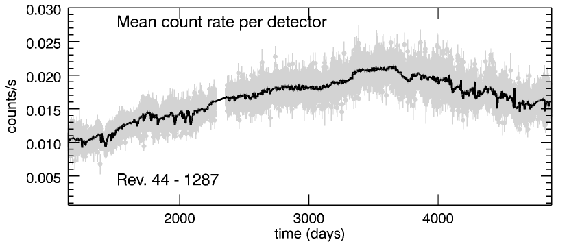
Figure 1.— Mean count rates recorded on the camera per detector versus time in the 1805-1813 keV energy band. In gray, the count rates and associated error bars (1 point per exposure). In black, the count rates averaged per revolution. The total number of exposures is 76 789. The hole around days 2500 corresponds to exposures with no PSD information (Section 2).

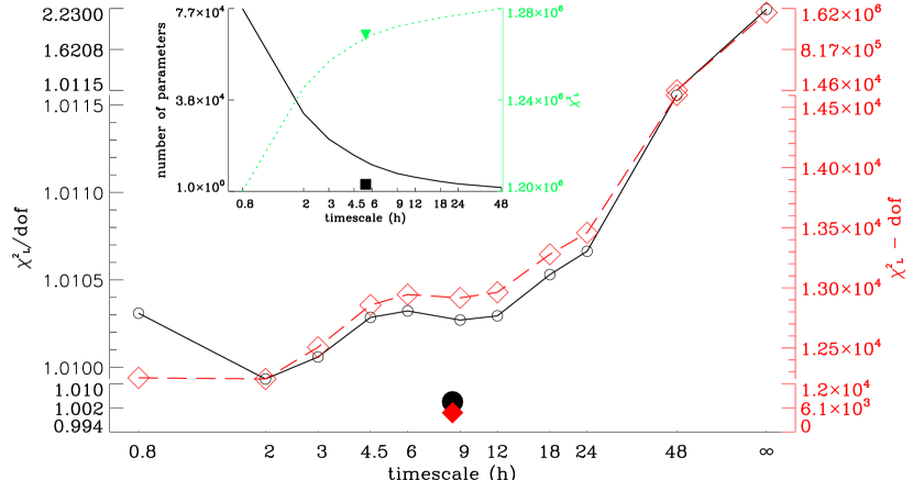
Figure 2.— A sky model, consisting of a synthetic map (here the 60$\mu$ map, Section 3.2), plus a few sources, is fitted to the 1805-1813 keV data (fixed-pattern method). The evolution of the reduced ($\chi^{2}_{L}/dof$) (solid-line, open black-circles) and the $\chi^{2}_{L}-dof$ (dashed-line, open red-diamonds) are shown as a function of the assumed background timescale (in hours). In insert are displayed the $\chi^{2}_{L}$ (dotted-green line) and the number of parameters to be determined (solid black line). The filled black-circle, red-diamond and (in insert) green triangle and black-square show respectively the $\chi^{2}_{L}/dof$, the $\chi^{2}_{L}-dof$ , the $\chi^{2}_{L}$ and the number of parameters obtained with the background segmentation method. The infinity symbol ($\infty$) on the x-axis corresponds to a constant background for the whole dataset.

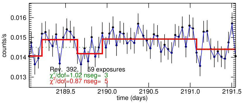
Figure 3.— Background intensity evolution in revolution 392. The background is modeled with 3 time-segments (dotted purple-line) to give a $\chi^{2}/dof$ of 1.02 or with 5 time-segments (red line) for a $\chi^{2}/dof$ of 0.87.

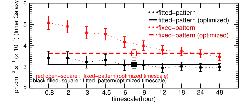
Figure 4.— Flux of the sky obtained with the fixed-pattern (open red-circles) and fitted-pattern (filled black-circles) background method as a function of the assumed background variation timescale (here using a 60$\mu$ map). The values obtained with the optimized number of background parameters are shown with the squares (open for fixed and filled for fitted-patter).

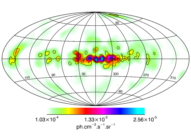
Figure 5.— Image of the ²⁶Al line (1805-1813 keV). The image is built with a resolution (ICF FWHM) of 6^∘. For this image reconstruction, the background pattern is adjusted as explained in Section 2.5.3. The contours are extracted from the 3^∘ resolution image. In units of $\times 10^{-3}$ ph cm^-2 s^-1 sr^-1, they correspond to 0.54, 1.1, and 2.7. Identified regions, from left to right: Perseus region (105^∘ $\leq$ l $\leq$ 170^∘) (Taurus clouds), Cygnus/Cepheus region (75^∘ $\leq$ l $\leq$ 100^∘), the inner Galaxy (-30^∘ $\leq$ l $\leq$30^∘, -10^∘ $\leq$ b $\leq$10^∘), Carina (l=286^∘, b=1^∘) and the Vela region (260^∘$\leq$ l $\leq$ 270^∘). At mid-latitude, the Sco/Cen region (300^∘ $\leq$ l $\leq$ 360^∘, 8 ^∘$\leq$ b $\leq$ 30^∘).

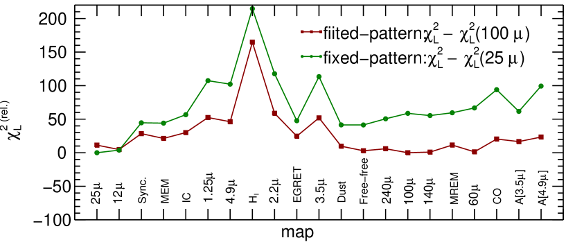
Figure 6.— The relative chi-square variation ($\chi^{2(rel.)}_{L})$ versus assumed template to model the distribution of the ²⁶Al line. $\chi^{2(rel.)}_{L})$ is the $\chi^{2}_{L}$ from which the value of the best fitted template is subtracted. The best template is the 100$\mu$ template for the fitted-pattern method ($\chi^{2}_{L}$=1258778.1 for 1261797 dof) and the 25$\mu$ template for the fixed-pattern method ($\chi^{2}_{L}$=1266968.4 for 1262208 dof). Terms: sync., dust and free-free, are abbreviations for 53 GHz synchrotron, dust and free-free maps described in Table 1. MEM and MREM indicate the COMPTEL maps, A[3.5$\mu$] and A[4.9$\mu$]corrected NIR extinction map. The red curve is for the fitted-pattern and green for fixed-pattern method. The maps are ordered following their contrast defined as the ratio of the flux enclosed in the region $|l|<150^{\circ}$, $|b|<15^{\circ}$ to the total flux.

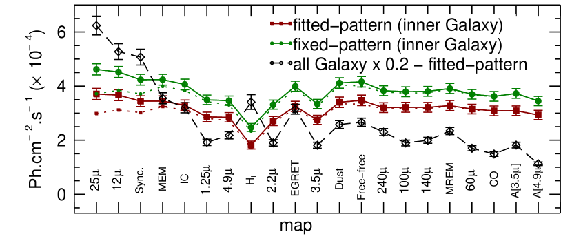
Figure 7.— Flux in the inner Galaxy as a function of the map used to model the distribution of the ²⁶Al line. The labels are the same as in Figure 6. The dashed black-curve is the total flux in the Galaxy (fitted-pattern), scaled by a factor 0.2. The dotted lines (red for fitted-pattern and green for fixed-pattern) are the fluxes obtained, if an isotropic emission (possibly extra-galactic) estimated by using the map emission at $|b|>$40^∘, is subtracted from each template. The labels are the same as in Figure 6.

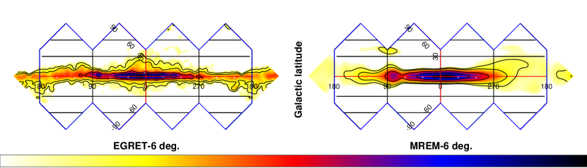
(a) Image template (shown at 6^∘ FWHM)

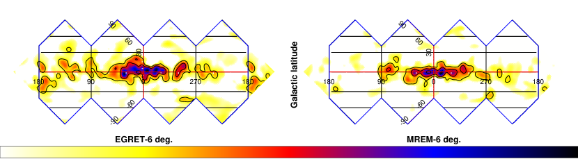
(b) Reconstruction 6^∘ FWHM

(c) Reconstruction 3^∘ FWHM

Figure 8.— Simulated and reconstructed maps. The image contains 49152 pixels (pixel size is 0.9^∘) ordered following the Healpix scheme. (Top) Simulated MREM (initially 3.8^∘) and EGRET (initially 2^∘) displayed using an angular resolution of 6^∘ FWHM. (Middle) The reconstructed MREM and EGRET fixing the output map resolution to 6^∘ FWHM and (Bottom) to 3^∘ FWHM. Images are displayed using the DS9 software (http://ds9.si.edu/site/Download.html). The images are scaled between their maximum intensity $f_{max}$ and $f_{max}/25$. The scale is in square root unit of the flux (ds9 Scale Square Root menu). (Top) contours correspond to $f_{max}/2$, $f_{max}/4$, $f_{max}/10$ and $f_{max}/16$. (Middle) $f_{max}/2$, $f_{max}/4$ and $f_{max}/10$. (Bottom) $f_{max}/5$ and $f_{max}/12$.

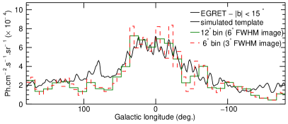
(a) EGRET simulated template

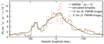
(b) MREM simulated template

Figure 9.— Longitude profiles of the reconstructed images compared to the simulated images (See Figure 8.

Table 1Maps used as templates.

	Tracer	Mechanism
${\dagger}$MIR 12 and 25$\mu$	warm dust (T$\sim$250 and $\sim$120 K)	dust nano-grains and PAHS
	/AGBs	heated to high temperature
${\dagger}$53 GHz sync	cosmic-rays/magnetic field	Synchroton
aCOMPTEL-MEM
IC	Inverse-Compton from GeV	Inverse-Compton
	electrons on the CMB and ISRF
${\dagger}$NIR 1.25, 4.9 $\mu$	stars (K and M giants)	star light
bHI (21 cm)	H hyperfine transition	Neutral hydrogen
${\dagger}$NIR 2.2$\mu$	stars (K and M giants)	star light
${\dagger}$EGRET	Interstellar gas/cosmic-rays	nuclear interactions
${\dagger}$NIR 3.5 $\mu$	stars (K and M giants)	star light
${\dagger}$53 GHz free-free	ionized gas	Free-free
${\dagger}$53 GHz dust	dust	Thermal dust
${\dagger}$FIR 100, 140 and 240$\mu$	warm dust (T $\sim$30,	microns sized dust emitting in thermal
	$\sim$21 and $\sim$12 K)	equilibrium with the heating ISRF
aCOMPTEL-MREM
${\dagger}$FIR 60$\mu$	warm dust (T$\sim$50 K)	microns sized dust emitting in thermal
		equilibrium with the heating ISRF
cCO	CO rotational transition	Molecular gas / young stars
dNIR extinction-corrected map	stars (K and M giants)	star light
3.5, 4.9 $\mu$ (hereafter A[${3.5\mu}$ and A[${4.9\mu}$] )

Note. — The maps are ordered in ascending “contrast”, defined here as the ratio between the fraction of the emission enclosed in the region $|l|<150^{\circ}$, $|b|<15^{\circ}$ to that of the whole sky. The value of the ratio varies from 0.4 (25$\mu$) to nearly 1 (A[${4.9\mu}$]).

${\dagger}$ available at http://lambda.gsfc.nasa.gov or http://heasarc.gsfc.nasa.gov.

The NIR, MIR and FIR maps are the COBE/DIRBE Zodi-Subtracted Mission Average (ZSMA) maps, from which zodiacal light contribution has been subtracted. Our 53 Ghz synchrotron presents some inaccuracies and is used for indicative purpose. ^a The maximum-entropy (MEM) and Multiresolution Regularized Expectation Maximization (MREM) all-sky image of the Galactic 1809 keV line emission observed with COMPTEL over 9 years (Plüschke et al., 2001, and references therein).^bDickey & Lockman (1990). ^cDame, Hartmann & Thaddeus (2001) with central peak removed (Section 2.3). ^dThe NIR extinction maps (Section 2.3).

Table 2²⁶Al emission sites and flux in units $\times$ 10^-5 ph cm^-2 s^-1.

Source	Position	Spatial	26Al large-scale morphology
name	l∘, b∘	morphology	IC map	A[${4.9\mu}$]
Cygnus region
Cyg OB2 clusterd	81,-1	Gaussian, $\sigma$=3	4.5 $\pm$ 1.5	4.1 $\pm$ 1.5
Mutiple sources - most significant excesses
	†81,-1	Gaussian, $\sigma$=3	4.3 $\pm$ 1.6	3.8 $\pm$ 1.6
	100, 6	Point-source	2.9 $\pm$ 1.1	2.7 $\pm$ 1.1
	†64, 1	Point-source	2.2 $\pm$ 1.1	2.0 $\pm$ 1.1
Sco-Cena,+	350, 20	disk r=10∘	0.4 $\pm$ 1.4	1.9 $\pm$ 1.4
	360, 16	disk r=5∘	0.5 $\pm$ 0.9	1.1 $\pm$ 0.9
Orion/Eridanus region
Orion/Eridanuse		150 $<$ l $<$ 210, -30 $<$ b $<$ 5	1.2 $\pm$ 3.2	0.5 $\pm$ 3.1
Carinab	∗287,0	disk r=3∘	3.1 $\pm$ 1.5	2.8 $\pm$ 1.5
Vela c	∗267,-1	disk r=4∘	3.6 $\pm$ 1.8	3.3 $\pm$ 1.8
Taurus†	∗161,-3	Disk r=5∘	5.6 $\pm$ 2.1	4.4 $\pm$ 2.1
	149, 8	Disk r=11∘	8.5 $\pm$ 2.9	7.9 $\pm$ 2.9
Other significant excesses
	226, 76	Gaussian, $\sigma$=3∘	7.2 $\pm$ 1.8	6.8 $\pm$ 1.8
Known high-energy emitting sources
Crab	185,-6	Point-source	1.2 $\pm$ 1.3	1.1 $\pm$ 1.3
Cyg X-1	71, 3	Point-source	0.2 $\pm$ 1.1	0.2 $\pm$ 1.1
PSR B1509-58	∗320,-1.2	Point-source	2.8 $\pm$ 0.9	2.8 $\pm$ 0.9

Note. — The first column contains the name of the source if it is known. The second column the position of the source in galactic coordinates and the third column the source spatial morphology; a point (point-source), an axi-symmetric Gaussian ($\sigma$ indicated) or a disk (radius indicated)). The position and spatial morphology in bold correspond to known sources or are based on published works. Next columns give the source fluxes obtained for two template maps used to model the large-scale distribution of ²⁶Al over the Galaxy; IC (low-contrast map) and A[${4.9\mu}$]  (high-contrast map). A model, comprising the ²⁶Al line distribution, the sources and the background, is adjusted to the data. The uncertainties are obtained from the model-fitting analysis by using the curvature matrix of the likelihood function and terms associated with the variance of the solution. The different labels identify excesses, which have been already mentioned in the literature by: ^a (Diehl et al., 2010) - ^b (Voss et al., 2012) - ^c (Diehl et al., 1995) - ^d(Martin et al., 2009) - ^e(Diehl et al., 2002).

^∗ Possible association with the spiral arms (Chen et al., 1996) - ^† Suspected or visible in COMPTEL ²⁶Al image (Oberlack et al., 1997; Plüschke et al., 2001). ⁺See Section 3.3.

Table 3Radioactive line fluxes in the inner Galaxy in units of $\times$10^-4 ph cm^-2 s^-1 .

	$25\mu$	COMPTEL-Al	$240\mu$	COMPTEL-MREM	$60\mu$	CO	${\dagger}$ A[${4.9\mu}$]
26Al	$3.68\pm 0.21$	$3.41\pm 0.20$	$3.15\pm 0.18$	$3.24\pm 0.19$	$3.11\pm 0.18$	$3.05\pm 0.18$	$2.92\pm 0.17$
60Fe	$0.47\pm 0.16$	$0.45\pm 0.15$	$0.38\pm 0.14$	$0.38\pm 0.14$	$0.38\pm 0.13$	$0.41\pm 0.13$	$0.42\pm 0.13$
60Fe/26Al	$0.13\pm 0.05$	$0.13\pm 0.05$	$0.12\pm 0.05$	$0.12\pm 0.05$	$0.12\pm 0.05$	$0.14\pm 0.05$	$0.15\pm 0.06$

Note. — Fluxes are given for the inner galaxy ($|l|<30^{\circ}$ and $|b|<10^{\circ}$). ${\dagger}$ the map is corrected from reddening and fluxes are essentially zero for $|b|>20^{\circ}$. ⁶⁰Fe is the average flux of the 1173 and 1333 keV lines (1170-1176 keV and 1330-1336 keV bands) and ²⁶Al the flux of the 1809 keV line in the 1805-1813 keV band. The fluxes are obtained using the “fitted-pattern” method.

References

- Bennett et al. (1992) Bennett, Smoot, G. F., Hinshaw, G., et al,, 1992, ApJ, 396, L7
- Bouchet et al. (2008) Bouchet, L., Jourdain, E., Roques, J. P, et al., 2008, ApJ, 679, 1315
- Bouchet et al. (2010) Bouchet, L., Roques, J. P., & Jourdain, E., 2010, ApJ, 720, 177
- Bouchet et al. (2011) Bouchet, L., Strong, A., Porter, T.A, et al., 2011, ApJ, 739, 29
- Bouchet et al. (2013a) Bouchet, L., Amestoy, P., Buttari, A, Rouet, F.-H. and Chauvin, M., 2013a, Astronomy and Computing, Volume 1, 59
- Bouchet et al. (2013b) Bouchet, L., Amestoy, P., Buttari, A, Rouet, F.-H. and Chauvin, M., 2013b,A&A, 555, 52
- Bryan & Skilling (1980) Bryan, R. K. & Skilling, J., 1980, MNRAS, 191, 69
- Cash (1979) Cash, W., 1979, ApJ, 228, 939
- Chen et al. (1996) Chen, W., Gehrels, N., Diehl, R. and Hartmann, D., 1996, A&AS, 120, 315
- Churazov et al. (2010) Churazov, E., Sazonov, S., Ysygankov S., et al., 2011, MNRAS, 411, 1727
- Dame, Hartmann & Thaddeus (2001) Dame, T. M., Hartmann, D. and Thaddeus, P., 2001, ApJ, 547, 792
- Dickey & Lockman (1990) Dickey, J. M., & Lockman, F. J. 1990, ARA&A , 28, 215
- Diehl et al. (1995) Diehl, R., Bennett, K., Bloemen, et al., 1995a, A&A, 298, L25
- Diehl et al. (1995) Diehl, R., Dupraz, C., Bennett, K., et al., 1995b, A&A, 298, 445
- Diehl et al. (2002) Diehl, R., 2002, New Astronomy Review, 46, 547
- Diehl et al. (2006) Diehl, R., Halloin, H., Kretschmer, K., et al., 2006, Nature, 439, 435
- Diehl et al. (2010) Diehl, R., Lang, M.G., Martin, P. et al., 2010, A&A, 522, A51
- Foster (1961) Foster, M., 1961, Journal of the Society for Industrial and Applied Mathematics 9 (3), 387
- Gorski et al. (2005) Górski, M., Hivon, E., Banday, A. J., et al., 2005, ApJ, 622, 759
- Gull (1989) Gull, S. F., 1989, in Skilling J., ed., Maximum Entropy and Bayesian Methods. Kluwer, Dordrecht, p. 53
- Harris et al. (2005) Harris, M. J, Knödlseder, J., Jean, P., et al., 2005, A&A, 433, L49
- Jensen et al. (2003) Jensen, P. L., Clausen, K., Cassi, C., et al., 2003, A&A, 411, L7
- Jourdain & Roques (2009) Jourdain, E. & Roques J. P., 2009, ApJ, 704, 17
- Knödlseder et al. (1996) Knödlseder, J., Bennett, K., Bloemen, H., et al., 1996, A&AS, 120, 327
- Knödlseder et al. (1999a) Knödlseder, J., Bennett, K., Bloemen, H., et al. 1999a, A&A, 344, 68
- Knödlseder et al. (1999b) Knödlseder, Dixon, D., J., Bennett, K., et al. 1999b, A&A, 345, 813
- Knödlseder et al. (2006) Knödlseder, J., Weidenspointner, G., Jean, P. et al., 2006, The Obscured Universe. Proceedings of the VI INTEGRAL Workshop, Editor: S. Grebenev, R. Sunyaev, C. Winkler. ESA SP-622, Noordwijk: ESA Publication Division, ISBN 92-9291-933-2, p 13
- Kretschmer et al. (2013) Kretschmer, K., Diehl, R., Krause, M. et al., 2013, aap, 559, 99
- Krivonos et al. (2007) Krivonos, R., Revnivtsev, M., Churazov, E., et al., 2007, A&A, 463, 957
- Limongi & Chieffi (2006) Limongi, M. & Chieffi, A. 2006, ApJ, 647, 483
- Mahoney et al. (1984) Mahoney, W. A., Ling J. C, Weathon, W. A. & Jacobson, A. S., 1984, ApJ,.286, 578
- Martin et al. (2009) Martin, P., Knödlseder, J., Diehl, R. & Meynet G., 2009 A&A, 506, 703
- Mighell (1999) Mighell, K. J., 1999, ApJ,518 380
- Oberlack et al. (1995) Oberlack, U., Bennett, K., Bloemen, H. et al., 1995, 24th International Cosmic Ray Conference, 2, 207
- Oberlack et al. (1997) Oberlack, U., Bennett, K., Bloemen, H., et al., 1996, A&AS, 120, 311
- Plüschke et al. (2000) Plüschke, S., Diehl, R., Schoenfelder, V., Weidenspointner, G, et al., 2000, The Fifth Compton Symposium, AIP Conference Proceedings, Volume 510,35
- Plüschke et al. (2001) Plüschke, S., Diehl, R., Schoenfelder, V., et al., 2001, ”Exploring the gamma-ray universe”, Proceedings of the Fourth INTEGRAL Workshop, Editor: B. Battrick, Scientific editors: A. Gimenez, V. Reglero & C. Winkler. ESA SP-459, Noordwijk: ESA Publications Division, ISBN 92-9092-677-5
- Prantzos & Diehl (1995) Prantzos, N. & Diehl, R., 1995, Advances in Space Research,15, 5, 99
- Roques et al. (2003) Roques, J. P., Schanne, S., Von Kienlin, A., et al., 2003, A&A, 411, L91
- Schoenfelder et al. (1993) Schoenfelder, V., Aarts, H., Bennett, K., et al., 1993, ApJS, 86, 657
- Skilling (1981) Skilling, J., 1981, Workshop on Maximum Entropy Estimation and Data Analysis, University of Wyoming, Reidel, Dordrecht, Holland
- Skilling & Bryan (1984) Skilling, J. & Bryan, R. K., 1984, MNRAS, 211, 111
- Smith (2004) Smith, D. M., 2004, ESA-SP-552, 45
- Timmes et al. (1995) Timmes, F. X., Woosley, S. E., Hartmann, D. H., et al. 1995, ApJ, 449, 20
- Tur, Heger & Austin (2010) Tur C., Heger,A. and Austin, S. M. 2010, ApJ, 718, 357
- Vedrenne et al. (2003) Vedrenne, G., Roques, J. P., Schonfelder, V., et al., 2003, A&A, 411, L63
- Voss et al. (2008) Voss, R.,Diehl, R., Hartmann, D. H and Kretschmer, K., 2008, New Astronomy Reviews, 52, 436
- Voss et al. (2010) Voss, R.,Diehl, R., Vink, J. S. and Hartmann, D. H, 2010, A&A, 520, 51
- Voss et al. (2012) Voss, R., Martin, P., Diehl, R., et al., 2012, A&A, 539, 66
- Wang et al. (2007) Wang, W., Harris, M. J., Diehl, R., et al., 2007, A&A, 469, 1005
- Wang et al. (2009) Wang, W., Lang, M. G., Diehl, R., et al., 2009, A&A, 496, 713
- Weidenspointner et al. (2008) Weidenspointner, G., Skinner, G., Jean, P., et al., 2008, Nature, 451, 159
- Woosley & Heger (2007) Woosley, S. E., & Heger, A., 2007, Phys. Rep., 442, 269