Computing the Rank Profile Matrix

Abstract

The row (resp. column) rank profile of a matrix describes the stair-case shape of its row (resp. column) echelon form. In an ISSAC’13 paper, we proposed a recursive Gaussian elimination that can compute simultaneously the row and column rank profiles of a matrix as well as those of all of its leading sub-matrices, in the same time as state of the art Gaussian elimination algorithms. Here we first study the conditions making a Gaussian elimination algorithm reveal this information. Therefore, we propose the definition of a new matrix invariant, the rank profile matrix, summarizing all information on the row and column rank profiles of all the leading sub-matrices. We also explore the conditions for a Gaussian elimination algorithm to compute all or part of this invariant, through the corresponding PLUQ decomposition. As a consequence, we show that the classical iterative CUP decomposition algorithm can actually be adapted to compute the rank profile matrix. Used, in a Crout variant, as a base-case to our ISSAC’13 implementation, it delivers a significant improvement in efficiency. Second, the row (resp. column) echelon form of a matrix are usually computed via different dedicated triangular decompositions. We show here that, from some PLUQ decompositions, it is possible to recover the row and column echelon forms of a matrix and of any of its leading sub-matrices thanks to an elementary post-processing algorithm.

1 Introduction

Triangular matrix decompositions are widely used in computational linear algebra. Besides solving linear systems of equations, they are also used to compute other objects more specific to exact arithmetic: computing the rank, sampling a vector from the null-space, computing echelon forms and rank profiles.

The row rank profile (resp. column rank profile) of an $m\times n$ matrix $A$ with rank $r$, denoted by RowRP(A) (resp. ColRP(A)), is the lexicographically smallest sequence of $r$ indices of linearly independent rows (resp. columns) of $A$. An $m\times n$ matrix has generic row (resp. column) rank profile if its row (resp. column) rank profile is $(1,..,r)$. Lastly, an $m\times n$ matrix has generic rank profile if its $r$ first leading principal minors are non-zero. Note that if a matrix has generic rank profile, then its row and column rank profiles are generic, but the converse is false: the matrix $\begin{bmatrix}0&1\\ 1&0\end{bmatrix}$ does not have generic rank profile even if its row and column rank profiles are generic. The row support (resp. column support) of a matrix $A$, denoted by $\text{RowSupp}({A})$ (resp. $\text{ColSupp}({A})$), is the subset of indices of its non-zero rows (resp. columns).

We recall that the row echelon form of an $m\times n$ matrix $A$ is an upper triangular matrix $E=TA$, for a non-singular matrix $T$, with the zero rows of $E$ at the bottom and the non-zero rows in stair-case shape: $\min\{j:a_{i,j}\neq 0\}<\min\{j:a_{i+1,j}\neq 0\}$. As $T$ is non singular, the column rank profile of $A$ is that of $E$, and therefore corresponds to the column indices of the leading elements in the staircase. Similarly the row rank profile of $A$ is composed of the row indices of the leading elements in the staircase of the column echelon form of $A$.

Rank profile and triangular matrix decompositions

The rank profiles of a matrix and the triangular matrix decomposition obtained by Gaussian elimination are strongly related. The elimination of matrices with arbitrary rank profiles gives rise to several matrix factorizations and many algorithmic variants. In numerical linear algebra one often uses the PLUQ decomposition, with $P$ and $Q$ permutation matrices, $L$ a lower unit triangular matrix and $U$ an upper triangular matrix. The LSP and LQUP variants of [8] are used to reduce the complexity rank deficient Gaussian elimination to that of matrix multiplication. Many other algorithmic decompositions exist allowing fraction free computations [10], in-place computations [4, 9] or sub-cubic rank-sensitive time complexity [13, 9]. In [5] we proposed a Gaussian elimination algorithm with a recursive splitting of both row and column dimensions, and replacing row and column transpositions by rotations. This elimination can compute simultaneously the row and column rank profile while preserving the sub-cubic rank-sensitive time complexity and keeping the computation in-place.

In this paper we first study the conditions a PLUQ decomposition algorithm must satisfy in order to reveal the rank profile structure of a matrix. We introduce in section 2 the rank profile matrix $\mathcal{R}_{A}$, a normal form summarizing all rank profile information of a matrix and of all its leading sub-matrices. We then decompose, in section 3, the pivoting strategy of any PLUQ algorithm into two types of operations: the search of the pivot and the permutation used to move it to the main diagonal. We propose a new search and a new permutation strategy and show what rank profiles are computed using any possible combination of these operations and the previously used searches and permutations. In particular we show three new pivoting strategy combinations that compute the rank profile matrix and use one of them, an iterative Crout CUP with rotations, to improve the base case and thus the overall performance of exact Gaussian elimination. Second, we show that preserving both the row and column rank profiles, together with ensuring a monotonicity of the associated permutations, allows us to compute faster several other matrix decompositions, such as the LEU and Bruhat decompositions, and echelon forms.

In the following, $0_{m\times n}$ denotes the $m\times n$ zero matrix and $A_{i..j,k..l}$ denotes the sub-matrix of $A$ of rows between $i$ and $j$ and columns between $k$ and $l$. To a permutation $\sigma:\{1,\dots,n\}\rightarrow\{1,\dots,n\}$ we define the associated permutation matrix $P_{\sigma}$, permuting rows by left multiplication: the rows of $P_{\sigma}A$ are that of $A$ permuted by $\sigma$. Reciprocally, for a permutation matrix $P$, we denote by $\sigma_{P}$ the associated permutation.

2 The rank profile matrix

We start by introducing in Theorem 1 the rank profile matrix, that we will use throughout this document to summarize all information on the rank profiles of a matrix. From now on, matrices are over a field $\mathrm{K}$ and a valid pivot is a non-zero element.

Definition 1.

An $r$-sub-permutation matrix is a matrix of rank $r$ with only $r$ non-zero entries equal to one.

Lemma 1.

An $m\times n$ $r$-sub-permutation matrix has at most one non-zero entry per row and per column, and can be written $P\begin{bmatrix}I_{r}\\ &0_{(m-r)\times(n-r)}\end{bmatrix}Q$ where $P$ and $Q$ are permutation matrices.

Theorem 1.

Let $A\in\mathrm{K}^{m\times n}$. There exists a unique $m\times n$ $\text{rank}(A)$-sub-permutation matrix $\mathcal{R}_{A}$ of which every leading sub-matrix has the same rank as the corresponding leading sub-matrix of $A$. This sub-permutation matrix is called the rank profile matrix of $A$.

Proof.

We prove existence by induction on the row dimension of the leading submatrices.

If $A_{1,1..n}=0_{1\times n}$, setting $\mathcal{R}^{(1)}=0_{1\times n}$ satisfies the defining condition. Otherwise, let $j$ be the index of the leftmost invertible element in $A_{1,1..n}$ and set $\mathcal{R}^{(1)}=e_{j}^{T}$ the j-th $n$-dimensional row canonical vector, which satisfies the defining condition.

Now for a given $i\in\{1,\dots,m\}$, suppose that there is a unique $i\times n$ rank profile matrix $\mathcal{R}^{(i)}$ such that $\text{rank}(A_{1..i,1..j})=\text{rank}(\mathcal{R}_{1..i,1..j})$ for every $j\in\{1..n\}$. If $\text{rank}(A_{1..i+1,1..n})=\text{rank}(A_{1..i,1..n})$, then $\mathcal{R}^{(i+1)}=\begin{bmatrix}\mathcal{R}^{(i)}\\ 0_{1\times n}\end{bmatrix}$. Otherwise, consider $k$, the smallest column index such that $\text{rank}(A_{1..i+1,1..k})=\text{rank}(A_{1..i,1..k})+1$ and set $\mathcal{R}^{(i+1)}=\begin{bmatrix}\mathcal{R}^{(i)}\\ e_{k}^{T}\end{bmatrix}$. Any leading sub-matrix of $\mathcal{R}^{(i+1)}$ has the same rank as the corresponding leading sub-matrix of $A$: first, for any leading subset of rows and columns with less than $i$ rows, the case is covered by the induction; second define $\begin{bmatrix}B&u\\ v^{T}&x\end{bmatrix}=A_{1..i+1,1..k}$, where $u,v$ are vectors and $x$ is a scalar. From the definition of $k$, $v$ is linearly dependent with $B$ and thus any leading sub-matrix of $\begin{bmatrix}B\\ v^{T}\end{bmatrix}$ has the same rank as the corresponding sub-matrix of $\mathcal{R}^{(i+1)}$. Similarly, from the definition of $k$, the same reasoning works when considering more than $k$ columns, with a rank increment by $1$.
Lastly we show that $\mathcal{R}^{(i+1)}$ is a $r_{i+1}$-sub-permutation matrix. Indeed, $u$ is linearly dependent with the columns of $B$: otherwise, $\text{rank}(\begin{bmatrix}B&u\end{bmatrix})=\text{rank}(B)+1$. From the definition of $k$ we then have $\text{rank}(\begin{bmatrix}B&u\\ v^{T}&x\end{bmatrix})=rank(\begin{bmatrix}B&u\end{bmatrix})+1=\text{rank}(B)+2=\text{rank}(\begin{bmatrix}B\\ v^{T}\end{bmatrix})+2$ which is a contradiction. Consequently, the $k$-th column of $\mathcal{R}^{(i)}$ is all zero, and $\mathcal{R}^{(i+1)}$ is a $r$-sub-permutation matrix.

To prove uniqueness, suppose there exist two distinct rank profile matrices $\mathcal{R}^{(1)}$ and $\mathcal{R}^{(2)}$ for a given matrix $A$ and let $(i,j)$ be some coordinates where $\mathcal{R}_{1..i,1..j}^{(1)}\neq\mathcal{R}_{1..i,1..j}^{(2)}$ and $\mathcal{R}_{1..i-1,1..j-1}^{(1)}=\mathcal{R}_{1..i-1,1..j-1}^{(2)}$. Then, $\text{rank}(A_{1..i,1..j})=\text{rank}(\mathcal{R}_{1..i,1..j}^{(1)})\neq\text{rank}(\mathcal{R}_{1..i,1..j}^{(2)})=\text{rank}(A_{1..i,1..j})$ which is a contradiction. ∎

Example 1.

$A=\begin{bmatrix}2&0&3&0\\ 1&0&0&0\\ 0&0&4&0\\ 0&2&0&1\\ \end{bmatrix}$ has $\mathcal{R}_{A}=\begin{bmatrix}1&0&0&0\\ 0&0&1&0\\ 0&0&0&0\\ 0&1&0&0\end{bmatrix}$ for rank profile matrix over $\mathbb{Q}$.

Remark 1.

The matrix $E$ introduced in Malaschonok’s LEU decomposition [12, Theorem 1], is in fact the rank profile matrix. There, the existence of this decomposition was only shown for $m=n=2^{k}$, and no connection was made to the relation with ranks and rank profiles. This connection was made in [5, Corollary 1], and the existence of $E$ generalized to arbitrary dimensions $m$ and $n$. Finally, after proving its uniqueness here, we propose this definition as a new matrix normal form.

The rank profile matrix has the following properties:

Lemma 2.

Let $A$ be a matrix.

1. $\mathcal{R}_{A}$ is diagonal if $A$ has generic rank profile.

2. $\mathcal{R}_{A}$ is a permutation matrix if $A$ is invertible

3. $\text{RowRP}(A)=\text{RowSupp}({\mathcal{R}_{A}})$; $\text{ColRP}(A)=\text{ColSupp}({\mathcal{R}_{A}})$.

Moreover, for all $1\leq i\leq m$ and $1\leq j\leq n$, we have:

1. $\text{RowRP}(A_{1..i,1..j})=\text{RowSupp}({(\mathcal{R}_{A})_{1..i,1..j}})$

2. $\text{ColRP}(A_{1..i,1..j})=\text{ColSupp}({(\mathcal{R}_{A})_{1..i,1..j}})$,

These properties show how to recover the row and column rank profiles of $A$ and of any of its leading sub-matrix.

3 Ingredients of a PLUQ decomposition algorithm

Over a field, the LU decomposition generalizes to matrices with arbitrary rank profiles, using row and column permutations (in some cases such as the CUP, or LSP decompositions, the row permutation is embedded in the structure of the $C$ or $S$ matrices). However such PLUQ decompositions are not unique and not all of them will necessarily reveal rank profiles and echelon forms. We will characterize the conditions for a PLUQ decomposition algorithm to reveal the row or column rank profile or the rank profile matrix.

We consider the four types of operations of a Gaussian elimination algorithm in the processing of the $k$-th pivot:

Pivot search:

finding an element to be used as a pivot,

Pivot permutation:

moving the pivot in diagonal position $(k,k)$ by column and/or row permutations,

Update:

applying the elimination at position $(i,j)$:
$a_{i,j}\leftarrow a_{i,j}-a_{i,k}a_{k,k}^{-1}a_{k,j}$,

Normalization:

dividing the $k$-th row (resp. column) by the pivot.

Choosing how each of these operation is done, and when they are scheduled results in an elimination algorithm. Conversely, any Gaussian elimination algorithm computing a PLUQ decomposition can be viewed as a set of specializations of each of these operations together with a scheduling.

The choice of doing the normalization on rows or columns only determines which of $U$ or $L$ will be unit triangular. The scheduling of the updates vary depending on the type of algorithm used: iterative, recursive, slab or tiled block splitting, with right-looking, left-looking or Crout variants [2]. Neither the normalization nor the update impact the capacity to reveal rank profiles and we will thus now focus on the pivot search and the permutations.

Choosing a search and a permutation strategy fixes the matrices $P$ and $Q$ of the PLUQ decomposition obtained and, as we will see, determines the ability to recover information on the rank profiles. Once these matrices are fixed, the $L$ and the $U$ factors are unique. We introduce the pivoting matrix.

Definition 2.

The pivoting matrix of a PLUQ decomposition $A=PLUQ$ of rank $r$ is the $r$-sub-permutation matrix

$$\Pi_{P,Q}=P\begin{bmatrix}I_{r}\\ &0_{(m-r)\times(n-r)}\end{bmatrix}Q.$$

The $r$ non-zero elements of $\Pi_{P,Q}$ are located at the initial positions of the pivots in the matrix $A$. Thus $\Pi_{P,Q}$ summarizes the choices made in the search and permutation operations.

Pivot search

The search operation vastly differs depending on the field of application. In numerical dense linear algebra, numerical stability is the main criterion for the selection of the pivot. In sparse linear algebra, the pivot is chosen so as to reduce the fill-in produced by the update operation. In order to reveal some information on the rank profiles, a notion of precedence has to be used: a usual way to compute the row rank profile is to search in a given row for a pivot and only move to the next row if the current row was found to be all zeros. This guarantees that each pivot will be on the first linearly independent row, and therefore the row support of $\Pi_{P,Q}$ will be the row rank profile. The precedence here is that the pivot’s coordinates must minimize the order for the first coordinate (the row index). As a generalization, we consider the most common preorders of the cartesian product $\{1,\ldots m\}\times\{1,\ldots n\}$ inherited from the natural orders of each of its components and describe the corresponding search strategies, minimizing this preorder:

Row order:

$(i_{1},j_{1})\preceq_{\text{row}}(i_{2},j_{2})$ iff $i_{1}\leq i_{2}$: search for any invertible element in the first non-zero row.

Column order:

$(i_{1},j_{1})\preceq_{\text{col}}(i_{2},j_{2})$ iff $j_{1}\leq j_{2}$. search for any invertible element in the first non-zero column.

Lexicographic order:

$(i_{1},j_{1})\preceq_{\text{lex}}(i_{2},j_{2})$ iff $i_{1}<i_{2}$ or $i_{1}=i_{2}$ and $j_{1}\leq j_{2}$: search for the leftmost non-zero element of the first non-zero row.

Reverse lexicographic order:

$(i_{1},j_{1})\preceq_{\text{revlex}}(i_{2},j_{2})$ iff $j_{1}<j_{2}$ or $j_{1}=j_{2}$ and $i_{1}\leq i_{2}$: search for the topmost non-zero element of the first non-zero column.

Product order:

$(i_{1},j_{1})\preceq_{\text{prod}}(i_{2},j_{2})$ iff $i_{1}\leq i_{2}$ and $j_{1}\leq j_{2}$: search for any non-zero element at position $(i,j)$ being the only non-zero of the leading $(i,j)$ sub-matrix.

Example 2.

Consider the matrix $\begin{bmatrix}0&0&0&a&b\\ 0&c&d&e&f\\ g&h&i&j&k\\ l&m&n&o&p\end{bmatrix}$, where each literal is a non-zero element. The minimum non-zero elements for each preorder are the following:

Row order	$a,b$
Column order	$g,l$
Lexicographic order	$a$
Reverse lexic. order	$g$
Product order	$a,c,g$

Pivot permutation

The pivot permutation moves a pivot from its initial position to the leading diagonal. Besides this constraint all possible choices are left for the remaining values of the permutation. Most often, it is done by row or column transpositions, as it clearly involves a small amount of data movement. However, these transpositions can break the precedence relations in the set of rows or columns, and can therefore prevent the recovery of the rank profile information. A pivot permutation that leaves the precedence relations unchanged will be called $k$-monotonically increasing.

Definition 3.

A permutation of $\sigma\in\mathcal{S}_{n}$ is called $k$-monotonically increasing if its last $n-k$ values form a monotonically increasing sequence.

In particular, the last $n-k$ rows of the associated row-permutation matrix $P_{\sigma}$ are in row echelon form. For example, the cyclic shift between indices $k$ and $i$, with $k<i$ defined as $R_{k,i}=(1,\ldots,k-1,i,k,k+1,\ldots,i-1,i+1,\ldots,n)$, that we will call a $(k,i)$-rotation, is an elementary $k$-monotonically increasing permutation.

Example 3.

The $(1,4)$-rotation $R_{1,4}=(4,1,2,3)$ is a $1$-monotonically increasing permutation. Its row permutation matrix is $\begin{bmatrix}0&&&1\\ 1&&&\\ &1&&\\ &&1&0\\ \end{bmatrix}$. In fact, any $(k,i)$-rotation is a $k$-monotonically increasing permutation.

Monotonically increasing permutations can be composed as stated in Lemma 3.

Lemma 3.

If $\sigma_{1}\in\mathcal{S}_{n}$ is a $k_{1}$-monotonically increasing permutation and $\sigma_{2}\in\mathcal{S}_{k_{1}}\times\mathcal{S}_{n-k_{1}}$ a $k_{2}$-monotonically increasing permutation with $k_{1}<k_{2}$ then the permutation $\sigma_{2}\circ\sigma_{1}$ is a $k_{2}$-monotonically increasing permutation.

Proof.

The last $n-k_{2}$ values of $\sigma_{2}\circ\sigma_{1}$ are the image of a sub-sequence of $n-k_{2}$ values from the last $n-k_{1}$ values of $\sigma_{1}$ through the monotonically increasing function $\sigma_{2}$. ∎

Therefore an iterative algorithm, using rotations as elementary pivot permutations, maintains the property that the permutation matrices $P$ and $Q$ at any step $k$ are $k$-monotonically increasing. A similar property also applies with recursive algorithms.

4 How to reveal rank profiles

A PLUQ decomposition reveals the row (resp. column) rank profile if it can be read from the first $r$ values of the permutation matrix $P$ (resp. $Q$). Equivalently, by Lemma 2, this means that the row (resp. column) support of the pivoting matrix $\Pi_{P,Q}$ equals that of the rank profile matrix.

Definition 4.

The decomposition $A=PLUQ$ reveals:

1. the row rank profile if $\text{RowSupp}({\Pi_{P,Q}})=\text{RowSupp}({\mathcal{R}_{A}})$,

2. the col. rank profile if $\text{ColSupp}({\Pi_{P,Q}})=\text{ColSupp}({\mathcal{R}_{A}})$,

3. the rank profile matrix if $\Pi_{P,Q}=\mathcal{R}_{A}$.

Example 4.

$A=\begin{bmatrix}2&0&3&0\\ 1&0&0&0\\ 0&0&4&0\\ 0&2&0&1\\ \end{bmatrix}$ has $\mathcal{R}_{A}=\begin{bmatrix}1&0&0&0\\ 0&0&1&0\\ 0&0&0&0\\ 0&1&0&0\end{bmatrix}$ for rank profile matrix over $\mathbb{Q}$. Now the pivoting matrix obtained from a PLUQ decomposition with a pivot search operation following the row order (any column, first non-zero row) could be the matrix $\Pi_{P,Q}=\begin{bmatrix}0&0&1&0\\ 1&0&0&0\\ 0&0&0&0\\ 0&1&0&0\\ \end{bmatrix}$. As these matrices share the same row support, the matrix $\Pi_{P,Q}$ reveals the row rank profile of $A$.

Remark 2.

Example 4, suggests that a pivot search strategy minimizing row and column indices could be a sufficient condition to recover both row and column rank profiles at the same time, regardless the pivot permutation. However, this is unfortunately not the case. Consider for example a search based on the lexicographic order (first non-zero column of the first non-zero row) with transposition permutations, run on the matrix: $A=\begin{bmatrix}0&0&1\\ 2&3&0\\ \end{bmatrix}$. Its rank profile matrix is $\mathcal{R}_{A}=\begin{bmatrix}0&0&1\\ 1&0&0\end{bmatrix}$ whereas the pivoting matrix could be $\Pi_{P,Q}=\begin{bmatrix}0&0&1\\ 0&1&0\end{bmatrix}$, which does not reveal the column rank profile. This is due to the fact that the column transposition performed for the first pivot changes the order in which the columns will be inspected in the search for the second pivot.

We will show that if the pivot permutations preserve the order in which the still unprocessed columns or rows appear, then the pivoting matrix will equal the rank profile matrix. This is achieved by the monotonically increasing permutations.

Theorem 2 shows how the ability of a PLUQ decomposition algorithm to recover the rank profile information relates to the use of monotonically increasing permutations. More precisely, it considers an arbitrary step in a PLUQ decomposition where $k$ pivots have been found in the elimination of an $\ell\times p$ leading sub-matrix $A_{1}$ of the input matrix $A$.

Theorem 2.

Consider a partial PLUQ decomposition of an $m\times n$ matrix $A$:

$$A=P_{1}\begin{bmatrix}L_{1}\\ M_{1}&I_{m-k}\end{bmatrix}\begin{bmatrix}U_{1}&V_{1}\\ &H\end{bmatrix}Q_{1}$$

where $\begin{bmatrix}L_{1}\\ M_{1}\end{bmatrix}$ is $m\times k$ lower triangular and $\begin{bmatrix}U_{1}&V_{1}\end{bmatrix}$ is $k\times n$ upper triangular, and let $A_{1}$ be some $\ell\times p$ leading sub-matrix of $A$, for $\ell,p\geq k$. Let $H=P_{2}L_{2}U_{2}Q_{2}$ be a PLUQ decomposition of $H$. Consider the PLUQ decomposition

$$A=\underbrace{P_{1}\begin{bmatrix}I_{k}\\ &P_{2}\end{bmatrix}}_{P}\underbrace{\begin{bmatrix}L_{1}\\ P_{2}^{T}M_{1}&L_{2}\end{bmatrix}}_{L}\underbrace{\begin{bmatrix}U_{1}&V_{1}Q_{2}^{T}\\ &U_{2}\end{bmatrix}}_{U}\underbrace{\begin{bmatrix}I_{k}\\ &Q_{2}\end{bmatrix}Q_{1}}_{Q}.$$

Consider the following clauses:

1. $\text{RowRP}(A_{1})=\text{RowSupp}({\Pi_{P_{1},Q_{1}}})$

2. $\text{ColRP}(A_{1})=\text{ColSupp}({\Pi_{P_{1},Q_{1}}})$

3. $\mathcal{R}_{A_{1}}=\Pi_{P_{1},Q_{1}}$

4. $\text{RowRP}(H)=\text{RowSupp}({\Pi_{P_{2},Q_{2}}})$

5. $\text{ColRP}(H)=\text{ColSupp}({\Pi_{P_{2},Q_{2}}})$

6. $\mathcal{R}_{H}=\Pi_{P_{2},Q_{2}}$

1. $P_{1}^{T}$ is $k$-monotonically increasing or ($P_{1}^{T}$ is $\ell$-monotonically increasing and $p=n$)

2. $Q_{1}^{T}$ is $k$-monotonically increasing or ($Q_{1}^{T}$ is $p$-monotonically increasing and $\ell=m$)

Then,

1. if (i) or (ii) or (iii) then $H=\begin{bmatrix}0_{(\ell-k)\times(p-k)}&*\\ *&*\end{bmatrix}$

2. if (vii) then ((i) and (iv)) $\Rightarrow\text{RowRP}(A)=\text{RowSupp}({\Pi_{P,Q}})$;

3. if (viii) then ((ii) and (v)) $\Rightarrow\text{ColRP}(A)=\text{ColSupp}({\Pi_{P,Q}})$;

4. if (vii) and (viii) then (iii) and (vi) $\Rightarrow\mathcal{R}_{A}=\Pi_{P,Q}$.

Proof.

Let $P_{1}=\begin{bmatrix}P_{11}&E_{1}\end{bmatrix}$ and $Q_{1}=\begin{bmatrix}Q_{11}\\ F_{1}\end{bmatrix}$ where $E_{1}$ is $m\times(m-k)$ and $F_{1}$ is $(n-k)\times n$. On one hand we have

$$A = \underbrace{\begin{bmatrix}P_{11}&E_{1}\end{bmatrix}\begin{bmatrix}L_{1}\\ M_{1}\end{bmatrix}\begin{bmatrix}U_{1}&V_{1}\end{bmatrix}\begin{bmatrix}Q_{11}\\ F_{1}\end{bmatrix}}_{B}+E_{1}HF_{1}.$$ (1)

On the other hand,

$$\Pi_{P,Q} = P_{1}\begin{bmatrix}I_{k}\\ &P_{2}\end{bmatrix}\begin{bmatrix}I_{r}\\ &0_{(m-r)\times(n-r)}\end{bmatrix}\begin{bmatrix}I_{k}\\ &Q_{2}\end{bmatrix}Q_{1}$$

$$= P_{1}\begin{bmatrix}I_{k}\\ &\Pi_{P_{2},Q_{2}}\end{bmatrix}Q_{1}=\Pi_{P_{1},Q_{1}}+E_{1}\Pi_{P_{2},Q_{2}}F_{1}.$$

Let $\overline{A}_{1}=\begin{bmatrix}A_{1}&0\\ 0&0_{(m-\ell)\times(n-p)}\end{bmatrix}$ and denote by $B_{1}$ the $\ell\times p$ leading sub-matrix of $B$.

1. The clause (i) or (ii) or (iii) implies that all $k$ pivots of the partial elimination were found within the $\ell\times p$ sub-matrix $A_{1}$. Hence $\text{rank}(A_{1})=k$ and we can write $P_{1}=\begin{bmatrix}\begin{array}[]{c}P_{11}\\ 0_{(m-\ell)\times k}\end{array}&E_{1}\end{bmatrix}$ and $Q_{1}=\begin{bmatrix}Q_{11}&0_{k\times(n-p)}\\ \lx@intercol\hfil F_{1}\hfil\lx@intercol\end{bmatrix}$, and the matrix $A_{1}$ writes

   $$A_{1}=\begin{bmatrix}I_{\ell}&0\end{bmatrix}A\begin{bmatrix}I_{p}\\ 0\end{bmatrix}=B_{1}+\begin{bmatrix}I_{\ell}&0\end{bmatrix}E_{1}HF_{1}\begin{bmatrix}I_{p}\\ 0\end{bmatrix}.$$ (2)

   Now $\text{rank}(B_{1})=k$ as a sub-matrix of $B$ of rank $k$ and since

   $$B_{1} = \begin{bmatrix}P_{11}&\begin{bmatrix}I_{\ell}&0\end{bmatrix}\cdot E_{1}\end{bmatrix}\begin{bmatrix}L_{1}\\ M_{1}\end{bmatrix}\begin{bmatrix}U_{1}&V_{1}\end{bmatrix}\begin{bmatrix}Q_{11}\\ F_{1}\cdot\begin{bmatrix}I_{p}\\ 0\end{bmatrix}\end{bmatrix}$$

   $$= P_{11}L_{1}U_{1}Q_{11}+\begin{bmatrix}I_{\ell}&0\end{bmatrix}E_{1}M_{1}\begin{bmatrix}U_{1}&V_{1}\end{bmatrix}Q_{1}\begin{bmatrix}I_{p}\\ 0\end{bmatrix}$$

   where the first term, $P_{11}L_{1}U_{1}Q_{11}$, has rank $k$ and the second term has a disjoint row support.

   Finally, consider the term $\begin{bmatrix}I_{\ell}&0\end{bmatrix}E_{1}HF_{1}\begin{bmatrix}I_{p}\\ 0\end{bmatrix}$ of equation (2). As its row support is disjoint with that of the pivot rows of $B_{1}$, it has to be composed of rows linearly dependent with the pivot rows of $B_{1}$ to ensure that $\text{rank}(A_{1})=k$. As its column support is disjoint with that of the pivot columns of $B_{1}$, we conclude that it must be the zero matrix. Therefore the leading $(\ell-k)\times(p-k)$ sub-matrix of $E_{1}HF_{1}$ is zero.

2. From (a) we know that $A_{1}=B_{1}$. Thus $\text{RowRP}(B)=\text{RowRP}(A_{1})$. Recall that $A=B+E_{1}HF_{1}$. No pivot row of $B$ can be made linearly dependent by adding rows of $E_{1}HF_{1}$, as the column position of the pivot is always zero in the latter matrix. For the same reason, no pivot row of $E_{1}HF_{1}$ can be made linearly dependent by adding rows of $B$. From (i), the set of pivot rows of $B$ is $\text{RowRP}(A_{1})$, which shows that

   $$\text{RowRP}(A)=\text{RowRP}(A_{1})\cup\text{RowRP}(E_{1}HF_{1}).$$ (3)

   Let $\sigma_{E_{1}}:\{1..m-k\}\rightarrow\{1..m\}$ be the map representing the sub-permutation $E_{1}$ (i.e. such that $E_{1}[\sigma_{E_{1}}(i),i]=1\ \forall i$). If $P_{1}^{T}$ is $k$-monotonically increasing, the matrix $E_{1}$ has full column rank and is in column echelon form, which implies that

   $$\text{RowRP}(E_{1}HF_{1}) = \sigma_{E_{1}}(\text{RowRP}(HF_{1}))$$ (4)

   $$= \sigma_{E_{1}}(\text{RowRP}(H)),$$

   since $F_{1}$ has full row rank. If $P_{1}^{T}$ is $\ell$ monotonically increasing, we can write $E_{1}=\begin{bmatrix}E_{11}&E_{12}\end{bmatrix}$, where the $m\times(m-\ell)$ matrix $E_{12}$ is in column echelon form. If $p=n$, the matrix $H$ writes $H=\begin{bmatrix}0_{(\ell-k)\times(n-k)}\\ H_{2}\end{bmatrix}$. Hence we have $E_{1}HF_{1}=E_{12}H_{2}F_{1}$ which also implies

   $$\text{RowRP}(E_{1}HF_{1})=\sigma_{E_{1}}(\text{RowRP}(H)).$$

   From equation (4), the row support of $\Pi_{P,Q}$ is that of $\Pi_{P_{1},Q_{1}}+E_{1}\Pi_{P_{2},Q_{2}}F_{1}$, which is the union of the row support of these two terms as they are disjoint. Under the conditions of point (b), this row support is the union of $\text{RowRP}(A_{1})$ and $\sigma_{E_{1}}(\text{RowRP}(H))$, which is, from (4) and (3), $\text{RowRP}(A)$.

3. Similarly as for point (b).

4. From (a) we have still $A_{1}=B_{1}$. Now since $\text{rank}(B)=\text{rank}(B_{1})=\text{rank}(A_{1})=k$, there is no other non-zero element in $\mathcal{R}_{B}$ than those in $\mathcal{R}_{\overline{A}_{1}}$ and $\mathcal{R}_{B}=\mathcal{R}_{\overline{A}_{1}}$. The row and column support of $\mathcal{R}_{B}$ and that of $E_{1}HF_{1}$ are disjoint. Hence

   $$\mathcal{R}_{A}=\mathcal{R}_{\overline{A}_{1}}+\mathcal{R}_{E_{1}HF_{1}}.$$ (5)

   If both $P_{1}^{T}$ and $Q_{1}^{T}$ are $k$-monotonically increasing, the matrix $E_{1}$ is in column echelon form and the matrix $F_{1}$ in row echelon form. Consequently, the matrix $E_{1}HF_{1}$ is a copy of the matrix $H$ with $k$ zero-rows and $k$ zero-columns interleaved, which does not impact the linear dependency relations between the non-zero rows and columns. As a consequence

   $$\mathcal{R}_{E_{1}HF_{1}}=E_{1}\mathcal{R}_{H}F_{1}.$$ (6)

   Now if $Q_{1}^{T}$ is $k$-monotonically increasing, $P_{1}^{T}$ is $\ell$-monotonically increasing and $p=n$, then, using notations of point (b), $E_{1}HF_{1}=E_{12}H_{2}F_{1}$ where $E_{12}$ is in column echelon form. Thus $\mathcal{R}_{E_{1}HF_{1}}=E_{1}\mathcal{R}_{H}F_{1}$ for the same reason. The symmetric case where $Q_{1}^{T}$ is $p$-monotonically increasing and $\ell=m$ works similarly. Combining equations (4), (5) and (6) gives $\mathcal{R}_{A}=\Pi_{P,Q}$.

∎

5 Algorithms for rank profiles

Using Theorem 2, we deduce what rank profile information is revealed by a PLUQ algorithm by the way the Search and the Permutation operations are done. Table 1 summarizes these results, and points to instances known in the literature, implementing the corresponding type of elimination. More precisely, we first distinguish in this table the ability to compute the row or column rank profile or the rank profile matrix, but we also indicate whether the resulting PLUQ decomposition preserves the monotonicity of the rows or columns. Indeed some algorithm may compute the rank profile matrix, but break the precedence relation between the linearly dependent rows or columns, making it unusable as a base case for a block algorithm of higher level.

Search	Row Perm.	Col. Perm.	Reveals	Monotonicity	Instance
Row order	Transposition	Transposition	RowRP		[8, 9]
Col. order	Transposition	Transposition	ColRP		[11, 9]
Lexicographic	Transposition	Transposition	RowRP		[13]
	Transposition	Rotation	RowRP, ColRP, $\mathcal{R}$	Col.	here
	Rotation	Rotation	RowRP, ColRP, $\mathcal{R}$	Row, Col.	here
Rev. lexico.	Transposition	Transposition	ColRP		[13]
	Rotation	Transposition	RowRP, ColRP, $\mathcal{R}$	Row	here
	Rotation	Rotation	RowRP, ColRP, $\mathcal{R}$	Row, Col.	here
Product	Rotation	Transposition	RowRP	Row	here
	Transposition	Rotation	ColRP	Col	here
	Rotation	Rotation	RowRP, ColRP, $\mathcal{R}$	Row, Col.	[5]

Table 1: Pivoting Strategies revealing rank profiles

5.1 Iterative algorithms

We start with iterative algorithms, where each iteration handles one pivot at a time. Here Theorem 2 is applied with $k=1$, and the partial elimination represents how one pivot is being treated. The elimination of $H$ is done by induction.

Row and Column order Search

The row order pivot search operation is of the form: any non-zero element in the first non-zero row. Each row is inspected in order, and a new row is considered only when the previous row is all zeros. With the notations of Theorem 2, this means that $A_{1}$ is the leading $\ell\times n$ sub-matrix of $A$, where $\ell$ is the index of the first non-zero row of $A$. When permutations $P_{1}$ and $Q_{1}$, moving the pivot from position $(\ell,j)$ to $(k,k)$ are transpositions, the matrix $\Pi_{P_{1},Q_{1}}$ is the element $E_{\ell,j}$ of the canonical basis. Its row rank profile is $(\ell)$ which is that of the $\ell\times n$ leading sub-matrix $A_{1}$. Finally, the permutation $P_{1}$ is $\ell$-monotonically increasing, and Theorem 2 case (b) can be applied to prove by induction that any such algorithm will reveal the row rank profile: $\text{RowRP}(A)=\text{RowSupp}({\Pi_{P,Q}})$. The case of the column order search is similar.

Lexicographic order based pivot search

In this case the Pivot Search operation is of the form: first non-zero element in the first non-zero row. The lexicographic order being compatible with the row order, the above results hold when transpositions are used and the row rank profile is revealed. If in addition column rotations are used, $Q_{1}=R_{1,j}$ which is $1$-monotonically increasing. Now $\Pi_{P_{1},Q_{1}}=E_{\ell,j}$ which is the rank profile matrix of the $\ell\times n$ leading sub-matrix $A_{1}$ of $A$. Theorem 2 case (d) can be applied to prove by induction that any such algorithm will reveal the rank profile matrix: $\mathcal{R}_{A}=\Pi_{P,Q}$. Lastly, the use of row rotations, ensures that the order of the linearly dependent rows will be preserved as well. Algorithm 1 is an instance of Gaussian elimination with a lexicographic order search and rotations for row and column permutations.

The case of the reverse lexicographic order search is similar. As an example, the algorithm in [13, Algorithm 2.14] is based on a reverse lexicographic order search but with transpositions for the row permutations. Hence it only reveals the column rank profile.

Product order based pivot search

The search here consists in finding any non-zero element $A_{\ell,p}$ such that the $\ell\times p$ leading sub-matrix $A_{1}$ of $A$ is all zeros except this coefficient. If the row and column permutations are the rotations $R_{1,\ell}$ and $R_{1,p}$, we have $\Pi_{P_{1},Q_{1}}=E_{\ell,p}=\mathcal{R}_{A_{1}}$. Theorem 2 case (d) can be applied to prove by induction that any such algorithm will reveal the rank profile matrix: $\mathcal{R}_{A}=\Pi_{P,Q}$. An instance of such an algorithm is given in [5, Algorithm 2]. If $P_{1}$ (resp. $Q_{1}$) is a transposition, then Theorem 2 case (c) (resp. case (b)) applies to show by induction that the columns (resp. row) rank profile is revealed.

5.2 Recursive algorithms

A recursive Gaussian elimination algorithm can either split one of the row or column dimension, cutting the matrix in wide or tall rectangular slabs, or split both dimensions, leading to a decomposition into tiles.

Slab recursive algorihtms

Most algorithms computing rank profiles are slab recursive [8, 11, 13, 9]. When the row dimension is split, this means that the search space for pivots is the whole set of columns, and Theorem 2 applies with $p=n$. This corresponds to a either a row or a lexicographic order. From case( b), one shows that, with transpositions, the algorithm recovers the row rank profile, provided that the base case does. If in addition, the elementary column permutations are rotations, then case (d) applies and the rank profile matrix is recovered. Finally, if rows are also permuted by monotonically increasing permutations, then the PLUQ decomposition also respects the monotonicity of the linearly dependent rows and columns. The same reasoning holds when splitting the column dimension.

Tile recursive algorithms

Tile recursive Gaussian elimination algorithms [5, 12, 6] are more involved, especially when dealing with rank deficiencies, and we refer to [5] for a detailed description of such an algorithm. Here, the search area $A_{1}$ has arbitrary dimensions $\ell\times p$, often specialized as $m/2\times n/2$. As a consequence, the pivot search can not satisfy neither row, column, lexicographic or reverse lexicographic orders. Now, if the pivots selected in the elimination of $A_{1}$ minimizes the product order, then they necessarily also respect this order as pivots of the whole matrix $A$. Now, from (a), the remaining matrix $H$ writes $H=\begin{bmatrix}0_{(\ell-k)\times(p-k)}&H_{12}\\ H_{21}&H_{22}\end{bmatrix}$ and its elimination is done by two independent eliminations on the blocks $H_{12}$ and $H_{21}$, followed by some update of $H_{22}$ and a last elimination on it. Here again, pivots minimizing the row order on $H_{21}$ and $H_{12}$ are also pivots minimizing this order for $H$, and so are those of the fourth elimination. Now the block row and column permutations used in [5, Algorithm 1] to form the PLUQ decomposition are $r$-monotonically increasing. Hence, from case (d), the algorithm computes the rank profile matrix and preserves the monotonicity. If only one of the row or column permutations are rotations, then case (b) or (c) applies to show that either the row or the column rank profile is computed.

6 Rank profile matrix based triangularizations

6.1 LEU decomposition

The LEU decomposition introduced in [12] involves a lower triangular matrix $L$, an upper triangular matrix $U$ and a $r$-sub-permutation matrix $E$.

Theorem 3.

Let $A=PLUQ$ be a PLUQ decomposition revealing the rank profile matrix ($\Pi_{P,Q}=\mathcal{R}_{A}$). Then an LEU decomposition of $A$ with $E=\mathcal{R}_{A}$ is obtained as follows (only using row and column permutations):

$$A=\underbrace{P\begin{bmatrix}L&0_{m\times(n-r)}\end{bmatrix}P^{T}}_{\overline{L}}\underbrace{P\begin{bmatrix}I_{r}\\ &0\end{bmatrix}Q}_{E}\underbrace{Q^{T}\begin{bmatrix}U\\ 0_{(n-r)\times n}\end{bmatrix}Q}_{\overline{U}}$$ (7)

Proof.

First $E=P\begin{bmatrix}I_{r}\\ &0\end{bmatrix}Q=\Pi_{P,Q}=\mathcal{R}_{A}$. Then there only needs to show that $\overline{L}$ is lower triangular and $\overline{U}$ is upper triangular. Suppose that $\overline{L}$ is not lower triangular, let $i$ be the first row index such that $\overline{L}_{i,j}\neq 0$ for some $i<j$. First $j\in\text{RowRP}(A)$ since the non-zero columns in $\overline{L}$ are placed according to the first $r$ values of $P$. Remarking that $A=P\begin{bmatrix}L&0_{m\times(n-r)}\end{bmatrix}\begin{bmatrix}\lx@intercol\hfil U\hfil\lx@intercol\\ 0&I_{n-r}\end{bmatrix}Q$, and since right multiplication by a non-singular matrix does not change row rank profiles, we deduce that $\text{RowRP}(\Pi_{P,Q})=\text{RowRP}(A)=\text{RowRP}(\overline{L})$. If $i\notin\text{RowRP}(A)$, then the $i$-th row of $\overline{L}$ is linearly dependent with the previous rows, but none of them has a non-zero element in column $j>i$. Hence $i\in\text{RowRP}(A)$.

Let $(a,b)$ be the position of the coefficient $\overline{L}_{i,j}$ in $L$, that is $a=\sigma_{P}^{-1}(i),b=\sigma_{P}^{-1}(j)$. Let also $s=\sigma_{Q}(a)$ and $t=\sigma_{Q}(b)$ so that the pivots at diagonal position $a$ and $b$ in $L$ respectively correspond to ones in $\mathcal{R}_{A}$ at positions $(i,s)$ and $(j,t)$. Consider the $\ell\times p$ leading sub-matrices $A_{1}$ of $A$ where $\ell=\max_{x=1..a-1}(\sigma_{P}(x))$ and $p=\max_{x=1..a-1}(\sigma_{Q}(x))$. On one hand $(j,t)$ is an index position in $A_{1}$ but not $(i,s)$, since otherwise $\text{rank}(A_{1})=b$. Therefore, $(i,s)\nprec_{prod}(j,t)$, and $s>t$ as $i<j$. As coefficients $(j,t)$ and $(i,s)$ are pivots in $\mathcal{R}_{A}$ and $i<j$ and $t<s$, there can not be a non-zero element above $(j,t)$ at row $i$ when it is chosen as a pivot. Hence $\overline{L}_{i,j}=0$ and $\overline{L}$ is lower triangular. The same reasoning applies to show that $\overline{U}$ is upper triangular. ∎

Remark 3.

Note that the LEU decomposition with $E=\mathcal{R}_{A}$ is not unique, even for invertible matrices. As a counter-example, the following decomposition holds for any $a\in\mathrm{K}$:

$$\left[\begin{matrix}0&1\\ 1&0\end{matrix}\right]=\left[\begin{matrix}1&0\\ a&1\end{matrix}\right]\left[\begin{matrix}0&1\\ 1&0\end{matrix}\right]\left[\begin{matrix}1&-a\\ 0&1\end{matrix}\right]$$ (8)

6.2 Bruhat decomposition

The Bruhat decomposition, that has inspired Malaschonok’s LEU decomposition [12], is another decomposition with a central permutation matrix [1, 7].

Theorem 4 ([1]).

Any invertible matrix $A$ can be written as $A=VPU$ for $V$ and $U$ uppper triangular invertible matrices and $P$ a permutation matrix. The latter decomposition is called the Bruhat decomposition of $A$.

It was then naturally extended to singular square matrices by [7]. Corollary 1 generalizes it to matrices with arbitrary dimensions, and relates it to the PLUQ decomposition.

Corollary 1.

Any $m\times n$ matrix of rank $r$ has a $VPU$ decomposition, where $V$ and $U$ are upper triangular matrices, and $P$ is a $r$-sub-permutation matrix.

Proof.

Let $J_{n}$ be the unit anti-diagonal matrix. From the LEU decomposition of $J_{n}A$, we have $A=\underbrace{J_{n}LJ_{n}}_{V}\underbrace{J_{n}E}_{P}U$ where $V$ is upper triangular. ∎

6.3 Relation to LUP and PLU decompositions

The LUP decomposition $A=LUP$ only exists for matrices with generic row rank profile (including matrices with full row rank). Corollary 2 shows upon which condition the permutation matrix $P$ equals the rank profile matrix $\mathcal{R}_{A}$. Note that although the rank profile $A$ is trivial in such cases, the matrix $\mathcal{R}_{A}$ still carries important information on the row and column rank profiles of all leading sub-matrices of $A$.

Corollary 2.

Let $A$ be an $m\times n$ matrix.

If $A$ has generic column rank profile, then any PLU decomposition $A=PLU$ computed using reverse lexicographic order search and row rotations is such that $\mathcal{R}_{A}=P\begin{bmatrix}I_{r}\\ &0\end{bmatrix}$. In particular, $P=\mathcal{R}_{A}$ if $r=m$.

If $A$ has generic row rank profile, then any LUP decomposition $A=LUP$ computed using lexicographic order search and column rotations is such that $\mathcal{R}_{A}=\begin{bmatrix}I_{r}\\ &0\end{bmatrix}P$. In particular, $P=\mathcal{R}_{A}$ if $r=n$.

Proof.

Consider $A$ has generic column rank profile. From table 1, any PLUQ decomposition algorithm with a reverse lexicographic order based search and rotation based row permutation is such that $\Pi_{P,Q}=P\begin{bmatrix}I_{r}\\ &\end{bmatrix}Q=\mathcal{R}_{A}$. Since the search follows the reverse lexicographic order and the matrix has generic column rank profile, no column will be permuted in this elimination, and therefore $Q=I_{n}$. The same reasoning hold for when $A$ has generic row rank profile. ∎

Note that the $L$ and $U$ factors in a PLU decomposition are uniquely determined by the permutation $P$. Hence, when the matrix has full row rank, $P=\mathcal{R}_{A}$ and the decomposition $A=\mathcal{R}_{A}LU$ is unique. Similarly the decomposition $A=LU\mathcal{R}_{A}$ is unique when the matrix has full column rank. Now when the matrix is rank deficient with generic row rank profile, there is no longer a unique PLU decomposition revealing the rank profile matrix: any permutation applied to the last $m-r$ columns of $P$ and the last $m-r$ rows of $L$ yields a PLU decomposition where $\mathcal{R}_{A}=P\begin{bmatrix}I_{r}\\ &\end{bmatrix}$.

Lastly, we remark that the only situation where the rank profile matrix $\mathcal{R}_{A}$ can be read directly as a sub-matrix of $P$ or $Q$ is as in corollary 2, when the matrix $A$ has generic row or column rank profile. Consider a PLUQ decomposition $A=PLUQ$ revealing the rank profile matrix ($\mathcal{R}_{A}=P\begin{bmatrix}I_{r}\\ &\end{bmatrix}Q$) such that $\mathcal{R}_{A}$ is a sub-matrix of $P$. This means that $P=\mathcal{R}_{A}+S$ where $S$ has disjoint row and column support with $\mathcal{R}_{A}$. We have $\mathcal{R}_{A}=(\mathcal{R}_{A}+S)\begin{bmatrix}I_{r}\\ &\end{bmatrix}Q=(\mathcal{R}_{A}+S)\begin{bmatrix}Q_{1}\\ 0_{(n-r)\times n}\end{bmatrix}$. Hence $\mathcal{R}_{A}(I_{n}-\begin{bmatrix}Q_{1}\\ 0_{(n-r)\times n}\end{bmatrix})=S\begin{bmatrix}Q_{1}\\ 0_{(n-r)\times n}\end{bmatrix}$ but the row support of these matrices are disjoint, hence $\mathcal{R}_{A}\begin{bmatrix}0\\ I_{n-r}\end{bmatrix}=0$ which implies that $A$ has generic column rank profile. Similarly, one shows that $\mathcal{R}_{A}$ can be a sub-matrix of $Q$ only if $A$ has a generic row rank profile.

7 Improvements in practice

In our previous contribution [5], we identified the ability to recover the rank profile matrix via the use of the product order search and of rotations. Hence we proposed an implementation combining a tile recursive algorithm and an iterative base case, using these search and permutation strategies.

The analysis of sections 4 and 5 shows that other pivoting strategies can be used to compute the rank profile matrix, and preserve the monotonicity. We present here a new base case algorithm and its implementation over a finite field that we wrote in the FFLAS-FFPACK library. It is based on a lexicographic order search and row and column rotations. Moreover, the schedule of the update operations is that of a Crout elimination, for it reduces the number of modular reductions, as shown in [3, § 3.1]. Algorithm 1 summarizes this variant.

Algorithm 1 Crout variant of PLUQ with lexicographic search and column rotations

1:$k\leftarrow 1$

2:for $i=1\dots m$ do

3:     $A_{i,k..n}\leftarrow A_{i,k..n}-A_{i,1..k-1}\times A_{1..k-1,k..n}$

4:     if $A_{i,k..n}=0$ then

5:         Loop to next iteration

6:     end if

7:     Let $A_{i,s}$ be the left-most non-zero element of row $i$.

8:     $A_{i+1..m,s}\leftarrow A_{i+1..m,s}-A_{i+1..m,1..k-1}\times A_{1..k-1,s}$

9:     $A_{i+1..m,s}\leftarrow A_{i+1..m,s}/A_{i,s}$

10:     Bring $A_{*,s}$ to $A_{*,k}$ by column rotation

11:     Bring $A_{i,*}$ to $A_{k,*}$ by row rotation

12:     $k\leftarrow k+1$

13:end for

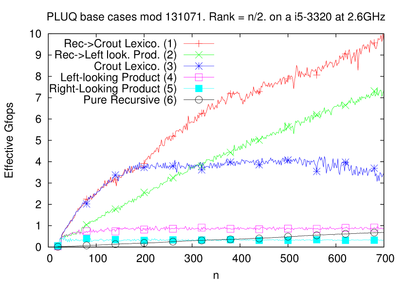
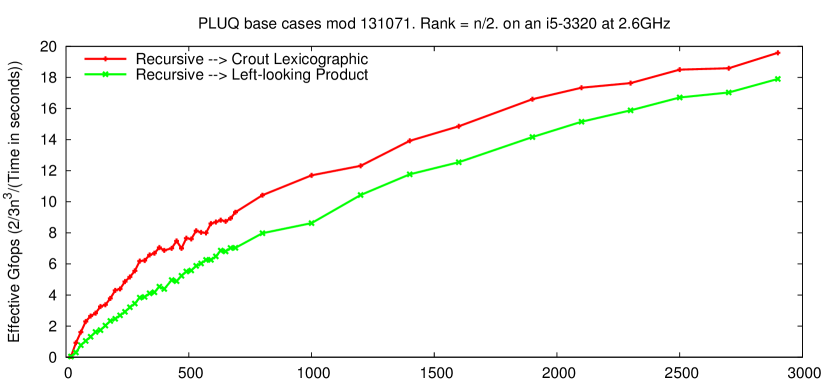
Figure 1: Computation speed of PLUQ decomposition base cases.

In the following experiments, we measured the real time of the computation averaged over 10 instances (100 for $n<500$) of $n\times n$ matrices with rank $r=n/2$ for any even integer value of $n$ between 20 and 700. In order to ensure that the row and column rank profiles of these matrices are uniformly random, we construct them as the product $A=L\mathcal{R}U$, where $L$ and $U$ are random non-singular lower and upper triangular matrices and $\mathcal{R}$ is an $m\times n$ $r$-sub-permutation matrix whose non-zero elements positions are chosen uniformly at random. The effective speed is obtained by dividing an estimate of the arithmetic cost ($2mnr+2/3r^{3}-r^{2}(m+n)$) by the computation time.

Figure 1 shows its computation speed (3), compared to that of the pure recursive algorithm (6), and to our previous base case algorithm [5], using a product order search, and either a left-looking (4) or a right-looking (5) schedule. At $n=200$, the left-looking variant (4) improves over the right looking variant (5) by a factor of about $2.14$ as it performs fewer modular reductions. Then, the Crout variant (3) again improves variant (4) by a factor of about 3.15. Lastly we also show the speed of the final implementation, formed by the tile recursive algorithm cascading to either the Crout base case (1) or the left-looking one (2). The threshold where the cascading to the base case occurs is experimentally set to its optimum value, i.e. 200 for variant (1) and 70 for variant (2). This illustrates that the gain on the base case efficiency leads to a higher threshold, and improves the efficiency of the cascade implementation (by an additive gain of about 2.2 effective Gfops in the range of dimensions considered).

8 Computing Echelon forms

Usual algorithms computing an echelon form [13, 9] use a slab block decomposition (with row or lexicographic order search), which implies that pivots appear in the order of the echelon form. The column echelon form is simply obtained as $C=PL$ from the PLUQ decomposition. Using product order search, this is no longer true, and the order of the columns in $L$ may not be that of the echelon form. Algorithm 2 shows how to recover the echelon form in such cases.

Algorithm 2 Echelon form from a PLUQ decomposition

1:$P,L,U,Q$, a PLUQ decomp. of $A$ with $\mathcal{R}_{A}=\Pi_{P,Q}$

2:$C$: the column echelon form of $A$

3:$C\leftarrow PL$

4:$(p_{1},..,p_{r})=\text{Sort}(\sigma_{P}(1),..,\sigma_{P}(r))$

5:for $i=1..r$ do

6:     $\tau=(\sigma_{P}^{-1}(p_{1}),..,\sigma_{P}^{-1}(p_{r}),r+1,..,m)$

7:end for

8:$C\leftarrow CP_{\tau}$

Note that both the row and the column echelon forms can thus be computed from the same PLUQ decomposition. Lastly, the column echelon form of the $i\times j$ leading sub-matrix, is computed by removing rows of $PL$ below index $i$ and filtering out the pivots of column index greater than $j$. The latter is achieved by replacing line 4 by $(p_{1},..,p_{s})=\text{Sort}(\{\sigma_{P}(i):\sigma_{Q}(i)\leq j\})$.

References

- [1] N. Bourbaki. Groupes et Algègres de Lie. Number Chapters 4–6 in Elements of mathematics. Springer, 2008.
- [2] J. J. Dongarra, L. S. Duff, D. C. Sorensen, and H. A. V. Vorst. Numerical Linear Algebra for High Performance Computers. SIAM, 1998.
- [3] J.-G. Dumas, T. Gautier, C. Pernet, and Z. Sultan. Parallel computation of echelon forms. In Euro-Par 2014 Parallel Proc., LNCS (8632), pages 499–510. Springer, 2014. doi:10.1007/978-3-319-09873-9_42.
- [4] J.-G. Dumas, P. Giorgi, and C. Pernet. Dense linear algebra over prime fields. ACM TOMS, 35(3):1–42, Nov. 2008. doi:10.1145/1391989.1391992.
- [5] J.-G. Dumas, C. Pernet, and Z. Sultan. Simultaneous computation of the row and column rank profiles. In M. Kauers, editor, Proc. ISSAC’13. ACM Press, 2013. URL: http://hal.archives-ouvertes.fr/hal-00778136, doi:10.1145/2465506.2465517.
- [6] J.-G. Dumas and J.-L. Roch. On parallel block algorithms for exact triangularizations. Parallel Computing, 28(11):1531–1548, Nov. 2002. doi:10.1016/S0167-8191(02)00161-8.
- [7] D. Y. Grigor’ev. Analogy of Bruhat decomposition for the closure of a cone of Chevalley group of a classical serie. Soviet Mathematics Doklady, 23(2):393–397, 1981.
- [8] O. H. Ibarra, S. Moran, and R. Hui. A generalization of the fast LUP matrix decomposition algorithm and applications. J. of Algorithms, 3(1):45–56, 1982. doi:10.1016/0196-6774(82)90007-4.
- [9] C.-P. Jeannerod, C. Pernet, and A. Storjohann. Rank-profile revealing Gaussian elimination and the CUP matrix decomposition. J. Symbolic Comput., 56:46–68, 2013. URL: http://dx.doi.org/10.1016/j.jsc.2013.04.004, doi:10.1016/j.jsc.2013.04.004.
- [10] D. J. Jeffrey. LU factoring of non-invertible matrices. ACM Comm. Comp. Algebra, 44(1/2):1–8, July 2010. URL: http://www.apmaths.uwo.ca/~djeffrey/Offprints/David-Jeffrey-LU.pdf, doi:10.1145/1838599.1838602.
- [11] W. Keller-Gehrig. Fast algorithms for the characteristic polynomial. Th. Comp. Science, 36:309–317, 1985. doi:10.1016/0304-3975(85)90049-0.
- [12] G. I. Malaschonok. Fast generalized Bruhat decomposition. In CASC’10, volume 6244 of LNCS, pages 194–202. Springer-Verlag, Berlin, Heidelberg, 2010.
- [13] A. Storjohann. Algorithms for Matrix Canonical Forms. PhD thesis, ETH-Zentrum, Zürich, Switzerland, Nov. 2000. doi:10.3929/ethz-a-004141007.