Line defects in the small elastic constant limit
of a three-dimensional Landau-de Gennes model

Abstract

We consider the Landau-de Gennes variational model for nematic liquid crystals, in three-dimensional domains. More precisely, we study the asymptotic behaviour of minimizers as the elastic constant tends to zero, under the assumption that minimizers are uniformly bounded and their energy blows up as the logarithm of the elastic constant. We show that there exists a closed set $\mathscr{S}_{\mathrm{line}}$ of finite length, such that minimizers converge to a locally harmonic map away from $\mathscr{S}_{\mathrm{line}}$. Moreover, $\mathscr{S}_{\mathrm{line}}$ restricted to the interior of the domain is a locally finite union of straight line segments. We provide sufficient conditions, depending on the domain and the boundary data, under which our main results apply. We also discuss some examples.

Keywords. Landau-de Gennes model, $Q$-tensors, asymptotic analysis, topological singularities, line defects, rectifiable sets, stationary varifolds.
2010 Mathematics Subject Classification. 76A15, 35J57, 35B40, 35A20.

1 Introduction

1.1 Variational theories for nematic liquid crystals

A nematic liquid crystal is matter in an intermediate state between liquid and crystalline solid. Molecules can flow and their centers of mass are randomly distributed, but the molecular axes tend to self-align locally. As a result, the material is anisotropic with respect to optic and electromagnetic properties. In the so-called uniaxial nematics, the molecules are often rod-shaped and, although they may carry a permanent dipole, there are as many dipoles ‘up’ as there are ‘down’. Therefore, the material symmetry group contains the rotations around the molecular axis and the reflection symmetry which exchanges the two orientations of the axis. The long-range orientational order due to the self-alignmennt of the molecules is broken in some places, called defects. The word nematic itself refers to the line defects (see Friedel, [32]):

I am going to use the term nematic ($\nu{\acute{\eta}}\mu\alpha$, thread) to describe the forms, bodies, phases, etc. of the second type… because of the linear discontinuities, which are twisted like threads, and which are one of their most prominent characteristics.

In addition to line defects, also called disclinations, nematic media exhibit “hedgehog-like” point singularities. According to the topological theory of ordered media (see e.g. [53, 63, 65]), both kinds of defects are described by the homotopy groups of a manifold, which parametrizes the possible local configurations of the material.

Several models for uniaxial nematic liquid crystals have drawn the attention of the mathematical community. The most popular continuum theories which are based on a finite-dimensional order parameter space are probably the Oseen-Frank, the Ericksen and the Landau-de Gennes theories. In the Oseen-Frank theory [31], the material is modeled by a unit vector field $\mathbf{n}=\mathbf{n}(x)\in\mathbb{S}^{2}$, which represents the preferred direction of molecular alignment. The elastic energy, in the simplest setting, reduces to the Dirichlet functional

(1) $$E(\mathbf{n}):=\frac{1}{2}\int_{\Omega}\left|\nabla\mathbf{n}\right|^{2},$$

where $\Omega\subseteq\mathbb{R}^{3}$ is the physical domain. In this case, least-energy configurations are but harmonic maps $\mathbf{n}\colon\Omega\to\mathbb{S}^{2}$. As such, minimizers have been widely studied in the literature (the reader is referred to e.g. [39] for a general review of this subject). Schoen and Uhlenbeck [60] proved that minimizers are smooth away from a discrete set of points singularities. Brezis, Coron and Lieb [17] investigated the precise shape of minimizers around a point defect $x_{0}$, and proved that

(2) $$\mathbf{n}(x)\simeq\pm R\frac{x-x_{0}}{|x-x_{0}|}\qquad\textrm{for }|x-x_{0}|\ll 1,$$

where $R$ is a rotation. These “hedgehog-like” point defects are associated with a non-trivial homotopy class of maps $\mathbf{n}\colon\partial B_{r}(x_{0})\to\mathbb{S}^{2}$, i.e. a non-trivial element of $\pi_{2}(\mathbb{S}^{2})$. Interesting results are also available for the full Oseen-Frank energy, which consists of various terms accounting for splay, twist and bend deformations. Hardt, Kinderlehrer and Lin [37] proved the existence of minimizers and partial regularity, i.e. regularity out of an exceptional set whose Hausdorff dimension is strictly less than $1$. As for the local behaviour of minimizers around the defects, the picture is not as clear as for the Dirichlet energy (1), but at least the stability of “hedgehog-like” singularities such as (2) as been completely analyzed (see [45] and the references therein). However, the partial regularity result of [37] implies that the Oseen-Frank theory cannot account for line defects.

Ericksen theory is less restrictive, because it allows variable orientational order. Indeed, the configurations are described by a pair $(s,\,\mathbf{n})\in\mathbb{R}\times\mathbb{S}^{2}$, where $\mathbf{n}$ is the preferred direction of molecular alignment and the scalar $s$ measures the degree of ordering. In this theory, defects are identified by the condition $s=0$, which correspond to complete disordered states. Under suitable assumptions, minimizers can exhibit line singularities and even planar discontinuities (see [47, Theorem 7.2]). Explicit examples were studied by Ambrosio and Virga [6] and Mizel, Roccato and Virga [54]. However, the Ericksen theory — as the Oseen-Frank theory — excludes configurations which might have physical reality. Ericksen himself was aware of this, since he presented his theory as a “kind of compromise” [29, p. 98] between physical intuition and mathematical simplicity. Indeed, both the Oseen-Frank and the Ericksen theory do not take into account the material symmetry, that is, the configurations represented by $\mathbf{n}$ and $-\mathbf{n}$ are physically indistinguishable. Moreover, these theories postulate that, at each point of the medium, there is at most one preferred direction of molecular orientation. Configurations for which such a preferred direction exists are called uniaxial, because they have one axis of rotational symmetry. If no preferred direction exists, the configuration is called isotropic (in the Ericksen theory, this corresponds to $s=0$).

The Landau-de Gennes theory [27] allows for a rather complete description of the local behaviour of the medium, because it accounts for biaxial configurations as well. A state is called biaxial when it has no axis of rotational symmetry, but three orthogonal axes of reflection symmetry instead (see [56] for more details). What makes the Landau-de Gennes theory so rich is the order parameter space. Configurations are described by matrices (the so-called $Q$-tensors), which can be interpreted as renormalized second-order moments of the microscopic distribution of molecules with respect to the orientation.

In this paper, we aim at describing the generation of line defects for nematics in three-dimensional domains from a variational point of view, within the Landau-de Gennes theory. Two main simplifying assumptions are postulated here. First, we neglect the effect of external electromagnetic fields. To induce non-trivial behaviour in minimizers, we couple the problem with non-homogeneous Dirichlet boundary conditions (strong anchoring). Second, we adopt the one-constant approximation, that is we drop out several terms in the expression of the elastic energy, and we are left with the gradient-squared term only. These assumptions, which drastically reduce the technicality of the problem, are common in the mathematical literature on this subject (see e.g. [28, 33, 40, 41, 46, 52]). For the two-dimensional case, the analysis of the analogous problem is presented in [21, 35].

1.2 The Landau-de Gennes functional

As we mentioned before, the local configurations of the medium are described by $Q$-tensors, i.e. elements of

$$\mathbf{S}_{0}:=\left\{Q\in\mathrm{M}_{3}(\mathbb{R})\colon Q^{\mathsf{T}}=Q,\ \operatorname{tr}Q=0\right\}.$$

This is a real linear space, of dimension five, which we endow with the scalar product $Q\cdot P:=Q_{ij}P_{ij}$ (Einstein’s convention is assumed). This choice of the configurations space can be justified as follows. At a microscopic scale, the distribution of molecules around a given point $x\in\Omega$, as a function of orientation, can be represented by a probability measure $\mu_{x}$ on the unit sphere $\mathbb{S}^{2}$. The measure $\mu_{x}$ satisfies to the condition $\mu_{x}(B)=\mu_{x}(-B)$ for all $B\in\mathscr{B}(\mathbb{S}^{2})$, which accounts for the head-to-tail symmetry of the molecules. Then, the simplest meaningful way to condense the information conveyed by $\mu_{x}$ is to consider the second-order moment

$$Q=\int_{\mathbb{S}^{2}}\left(\mathbf{n}^{\otimes 2}-\frac{1}{3}\operatorname{Id}\right)\mathrm{d}\mu_{x}(\mathbf{n}).$$

We denote by $\mathbf{n}^{\otimes 2}$ the matrix defined by $(\mathbf{n}^{\otimes 2})_{i,j}:=\mathbf{n}_{i}\mathbf{n}_{j}$, for each $i,\,j\in\{1,\,2,\,3\}$. The quantity $Q$ is renormalized, so that the isotropic state $\mu_{x}=\mathscr{H}^{2}\mathbin{\vrule height=6.88889pt,depth=0.0pt,width=0.55974pt\vrule height=0.55974pt,depth=0.0pt,width=5.59721pt}\mathbb{S}^{2}$ corresponds to $Q=0$. As a result, $Q$ is a symmetric traceless matrix. (The interested reader is referred e.g. to [56] for further details.)

The (simplified) Landau-de Gennes functional reads

(LG_ε) $$E_{\varepsilon}(Q):=\int_{\Omega}\left\{\frac{1}{2}\left|\nabla Q\right|^{2}+\frac{1}{\varepsilon^{2}}f(Q)\right\},$$

where $Q\colon\Omega\to\mathbf{S}_{0}$ is the configuration of the medium, located in a bounded container $\Omega\subseteq\mathbb{R}^{3}$. The function $f$ is the quartic Landau-de Gennes potential, defined by

(3) $$f(Q)=k-\frac{a}{2}\operatorname{tr}Q^{2}-\frac{b}{3}\operatorname{tr}Q^{3}+\frac{c}{4}\left(\operatorname{tr}Q^{2}\right)^{2}\qquad\textrm{for }Q\in\mathbf{S}_{0}.$$

This expression for $f$ has been derived by a formal expansion in powers of $Q$. All the terms are invariant by rotations so that $f$ is independent of the coordinate frame. This potential allows for multiple local minima, with a first-order isotropic-nematic phase transition (see [27, 64]). The positive parameters $a$, $b$ and $c$ depend on the material and the temperature (which is assumed to be uniform), whereas $k$ is just an additive constant, which plays no role in the minimization problem. The potential $f$ is bounded from below, so we determine uniquely the value of $k$ by requiring $\inf f=0$. The parameter $\varepsilon^{2}$ is a material-dependent elastic constant, typically very small. For each $0<\varepsilon<1$, we assign a boundary datum $g_{\varepsilon}\in H^{1}(\partial\Omega,\,\mathbf{S}_{0})$ and we restrict our attention to minimizers $Q_{\varepsilon}$ of (LG_ε) in the class

$$H^{1}_{g_{\varepsilon}}(\Omega,\,\mathbf{S}_{0}):=\left\{Q\in H^{1}(\Omega,\,\mathbf{S}_{0})\colon Q=g_{\varepsilon}\textrm{ on }\partial\Omega\textrm{ in the sense of traces}\right\}.$$

When $\varepsilon$ is small, the term $\varepsilon^{-2}f(Q)$ in (LG_ε) forces minimizers to take their values close to $\mathscr{N}:=f^{-1}(0)$. This set can be characterized as follows (see [52, Proposition 9]):

(4) $$\mathscr{N}=\left\{s_{*}\left(\mathbf{n}^{\otimes 2}-\frac{1}{3}\operatorname{Id}\right)\colon\mathbf{n}\in\mathbb{S}^{2}\right\},$$

where the constant $s_{*}$ is defined by

$$s_{*}=s_{*}(a,\,b,\,c):=\frac{1}{4c}\left(b+\sqrt{b^{2}+24ac}\right).$$

Thus, $\mathscr{N}$ is a smooth submanifold of $\mathbf{S}_{0}$, diffeomorphic to the real projective plane $\mathbb{RP}^{2}$, called vacuum manifold. The topology of $\mathscr{N}$ plays an important role, for a map $\Omega\to\mathscr{N}$ may encounter topological obstructions to regularity. Sources of obstruction are the homotopy groups $\pi_{1}(\mathscr{N})\simeq\mathbb{Z}/2\mathbb{Z}$ and $\pi_{2}(\mathscr{N})\simeq\mathbb{Z}$, which are associated with line and point singularities, respectively. There is a remarkable difference with the Oseen-Frank model at this level, for $\mathbb{S}^{2}$ is a simply connected manifold, so topological obstructions result from $\pi_{2}(\mathbb{S}^{2})$ only. Despite this fact, a strong connection between the Oseen-Frank and Landau-de Gennes theories was established by Majumdar and Zarnescu. In their paper [52], they addressed the asymptotic analysis of minimizers of (LG_ε), in three-dimensional domains. Their results imply that, when $\Omega$, $\partial\Omega$ are simply connected and $g_{\varepsilon}=g\in C^{1}(\partial\Omega,\,\mathscr{N})$, minimizers $Q_{\varepsilon}$ of (LG_ε) converge in $H^{1}(\Omega,\,\mathbf{S}_{0})$ to a map of the form

$$Q_{0}(x)=s_{*}\left(\mathbf{n}_{0}^{\otimes 2}(x)-\frac{1}{3}\operatorname{Id}\right)$$

where $\mathbf{n}_{0}\in H^{1}(\Omega,\,\mathbb{S}^{2})$ is a minimizer of (1). The convergence is locally uniform, away from singularities of ${Q}_{0}$. Also in this case, line defects do not appear in the limiting map, although point defects analogous to (2) might occur. Indeed, their assumptions on the domain and boundary datum are strong enough to guarantee the uniform energy bound

(5) $$E_{\varepsilon}(Q_{\varepsilon})\leq C$$

for an $\varepsilon$-independent constant $C$, and obtain $H^{1}$-compactness. In this paper, we work in the logarithmic energy regime

(6) $$E_{\varepsilon}(Q_{\varepsilon})\leq C\left(\left|\log\varepsilon\right|+1\right),$$

which is compatible with singularities of codimension two, in the small $\varepsilon$ limit.

There are analogies between the functional (LG_ε) and the Ginzburg-Landau energy for superconductivity, which reduces to

(7) $$E^{\mathrm{GL}}_{\varepsilon}(u):=\int_{\Omega}\left\{\frac{1}{2}\left|\nabla u\right|^{2}+\frac{1}{4\varepsilon^{2}}\left(1-|u|^{2}\right)^{2}\right\}$$

when no external field is applied. Here the unknown is a complex-valued function $u$. There is a rich literature about the asymptotic behaviour, as $\varepsilon\to 0$, of critical points satisfying a logarithmic energy bound such as (6). It is well-known that, under appropriate assumptions, critical points converge to maps with topology-driven singularities of codimension two. In two-dimensional domains, the theory has been developed after Bethuel, Brezis and Hélein’s work [11]. In the three-dimensional case, the asymptotic analysis of minimizers was performed by Lin and Rivière [48], and extended to non-minimizing critical points by Bethuel, Brezis and Orlandi [12]. Later, Jerrard and Soner [44] and Alberti, Baldo, Orlandi [1] proved independently that $|\log\varepsilon|^{-1}E_{\varepsilon}^{\mathrm{GL}}$ $\Gamma$-converges, when $\varepsilon\to 0$, to a functional on integral currents of codimension two. This functional essentially measures the length of defect lines, weighted by some quantity that accounts for the topology of the defect.

1.3 Main results

For each fixed $\varepsilon>0$, a classical argument of Calculus of Variations shows that minimizers of (LG_ε) exist as soon as $g_{\varepsilon}\in H^{1/2}(\partial\Omega,\,\mathbf{S}_{0})$ and are regular in the interior of the domain. Our main result deals with their asymptotic behaviour as $\varepsilon\to 0$.

Theorem 1.

Let $\Omega$ be a bounded, Lipschitz domain. Assume that there exists a positive constant $M$ such that, for any $0<\varepsilon<1$, there hold

(H) $$E_{\varepsilon}(Q_{\varepsilon})\leq M\left(\left|\log\varepsilon\right|+1\right)\qquad\textrm{and}\qquad\left\|Q_{\varepsilon}\right\|_{L^{\infty}(\Omega)}\leq M.$$

Then, there exist a subsequence $\varepsilon_{n}\searrow 0$, a closed set $\mathscr{S}_{\mathrm{line}}\subseteq\overline{\Omega}$ and a map ${Q}_{0}\in H^{1}_{\mathrm{loc}}(\Omega\setminus\mathscr{S}_{\mathrm{line}},\,\mathscr{N})$ such that the following holds.

1. $\mathscr{S}_{\mathrm{line}}\cap\Omega$ is a countably $\mathscr{H}^{1}$-rectifiable set, and $\mathscr{H}^{1}(\mathscr{S}_{\mathrm{line}}\cap\Omega)<+\infty$.

2. ${Q}_{\varepsilon_{n}}\to{Q}_{0}$ strongly in $H^{1}_{\mathrm{loc}}(\Omega\setminus\mathscr{S}_{\mathrm{line}},\,\mathscr{N})$.

3. ${Q}_{0}$ is locally minimizing harmonic in $\Omega\setminus\mathscr{S}_{\mathrm{line}}$, that is for every ball $B\subset\!\subset\Omega\setminus\mathscr{S}_{\mathrm{line}}$ and any $P\in H^{1}(B,\,\mathscr{N})$ which satisfies $P=Q_{0}$ on $\partial B$ we have

   $$\frac{1}{2}\int_{B}\left|\nabla{Q}_{0}\right|^{2}\leq\frac{1}{2}\int_{B}\left|\nabla P\right|^{2}.$$

4. There exists a locally finite set $\mathscr{S}_{\mathrm{pts}}\subseteq\Omega\setminus\mathscr{S}_{\mathrm{line}}$ such that ${Q}_{0}$ is smooth on $\Omega\setminus(\mathscr{S}_{\mathrm{line}}\cup\mathscr{S}_{\mathrm{pts}})$ and $Q_{\varepsilon}\to{Q}_{0}$ locally uniformly in $\Omega\setminus(\mathscr{S}_{\mathrm{line}}\cup\mathscr{S}_{\mathrm{pts}})$.

By saying that $\mathscr{S}_{\mathrm{line}}$ is countably $\mathscr{H}^{1}$-rectifiable we mean that there exists a decomposition

$$\mathscr{S}_{\mathrm{line}}=\bigcup_{j\in\mathbb{N}}\SS_{j},$$

where $\mathscr{H}^{1}(\SS_{0})=0$ and, for each $j\geq 1$, the set $\SS_{j}$ is the image of a Lipschitz function $\mathbb{R}\to\mathbb{R}^{3}$. In addition to the singular set $\mathscr{S}_{\mathrm{line}}$ of dimension one, the limiting map ${Q}_{0}$ may have a set of point singularities $\mathscr{S}_{\mathrm{pts}}$. This is consistent with the regularity results for minimizing harmonic maps [34, 60]. Later on, we will discuss examples where $\mathscr{S}_{\mathrm{line}}$ and $\mathscr{S}_{\mathrm{pts}}$ are non-empty.

Theorem 1 is local in nature. In particular, boundary conditions play no particular role in the proof of this result, although they need to be imposed to induce non-trivial behaviour of minimizers. Theorem 1 can be adapted to the analysis near the boundary of the domain, under additional assumptions on the boundary datum. The necessary modifications are sketched in Section 4.4.

The singular set $\mathscr{S}_{\mathrm{line}}$ is defined as the concentration set for the energy densities of minimizers. In other words, thanks to (H) we find a subsequence $\varepsilon_{n}\searrow 0$ and a measure $\mu_{0}\in\mathscr{M}_{\mathrm{b}}(\overline{\Omega}):=C(\overline{\Omega})^{\prime}$ such that

$$\left\{\frac{1}{2}\left|\nabla Q_{\varepsilon_{n}}\right|^{2}+\frac{1}{\varepsilon^{2}_{n}}f(Q_{\varepsilon_{n}})\right\}\frac{\mathrm{d}x}{|\log\varepsilon_{n}|}\rightharpoonup^{*}\mu_{0}\qquad\textrm{in }\mathscr{M}_{\mathrm{b}}(\overline{\Omega}),$$

then we define $\mathscr{S}_{\mathrm{line}}:=\mathrm{supp\,}\mu_{0}$. A more precise description of the limit measure $\mu_{0}$ is given by the following result. We set

$$\kappa_{*}:=\frac{\pi}{2}s_{*}^{2}.$$

As we will see in Section 2.2, this number quantifies the energy cost associated with a topological defect of codimension two.

Proposition 2.

The measure $\mu_{0}\mathbin{\vrule height=6.88889pt,depth=0.0pt,width=0.55974pt\vrule height=0.55974pt,depth=0.0pt,width=5.59721pt}\Omega$ is naturally associated with a stationary varifold, and

$$\lim_{r\to 0}\frac{\mu_{0}(\overline{B}_{r}(x))}{2r}=\kappa_{*}\qquad\textrm{for }\mu_{0}\textrm{-a.e. }x\in\Omega.$$

For any open set $K\subset\!\subset\Omega$, $\mathscr{S}_{\mathrm{line}}\cap\overline{K}$ is the union of a finite number of closed straight line segments $L_{1},\,\ldots,\,L_{p}$. After possible subdivision, assume that for each $i\neq j$, either $L_{i}$ and $L_{j}$ are disjoint or they intersect at a common endpoint. Then, the following properties hold.

1. If $D\subset\!\subset K$ is a closed disk which intersects $\mathscr{S}_{\mathrm{line}}$ at a single point $x_{0}$ and $x_{0}$ is not an endpoint for any $L_{i}$, then the homotopy class of $Q_{0}$ restricted to $\partial D$ is non-trivial.

2. Suppose that $x_{0}\in K$ is an endpoint of exactly $q$ segments $L_{i_{1}},\,\ldots,\,L_{i_{q}}$. Then $q$ is even.

The definition of stationary varifold is given in [62, Chapter 4]. Varifolds are a generalization of differentiable manifolds, introduced by Almgren [4] in the context of Calulus of Variations, and stationary varifolds can be though as a weak notion of minimal manifolds. Proposition 2 relies heavily on the structure theorem for stationary varifolds of dimension one [3, Theorem p. 89].

Inside the domain, the singular set is a locally finite union of line segments. Branching points are not excluded by this result, but only an even number of branches can originate from each point. (However, we expect that branching points should not arise — see the concluding remarks, Section 1.4.) Moreover, the set $\mathscr{S}_{\mathrm{line}}$ is a topological singularity, i.e. it is associated with a non-trivial homotopy class of the map $Q_{0}$. Therefore, from the physical point of view $\mathscr{S}_{\mathrm{line}}$ corresponds to the “thin disclination lines” of index $\pm 1/2$ (see, e.g. [22]). The “thick disclination lines” of index $\pm 1$ are not included in $\mathscr{S}_{\mathrm{line}}$ because the order parameter $Q_{0}$ can be defined continuously throughout their cores, thanks to the “escape in the third dimension” proposed by Cladis and Kléman [24]. Proposition 2 also excludes disclination loops in the interior of the domain, although loops of radius larger than some critical value $R_{c}$ are expected to occur (see [22, p. 519]). However, in the limit as $\varepsilon\to 0$ we have that $R_{c}\to+\infty$, therefore any defect loop which is contractible in $\Omega$ should become unstable, shrink and eventually disappear. On the other hand, disclination loops may occur at the boundary of the domain. In Section 5.4, we show by an example that the singular set $\mathscr{S}_{\mathrm{line}}$ may touch $\partial\Omega$, even if the boundary datum is smooth. In this case, the conclusion of Proposition 2 does not hold any more.

We provide sufficient conditions for the estimate (H) to hold, in terms of the domain and the boundary data. Here is our first condition.

1. $\Omega$ is a bounded, smooth domain and $\{g_{\varepsilon}\}_{0<\varepsilon<1}$ is a bounded family in $H^{1/2}(\partial\Omega,\,\mathscr{N})$.

The uniform $H^{1/2}$-bound is satisfied if, for instance, $g_{\varepsilon}=g\colon\partial\Omega\to\mathscr{N}$ has a finite number of disclinations. This means, there exists a finite set $\Sigma\subseteq\partial\Omega$ such that $g$ is smooth on $\partial\Omega\setminus\Sigma$ and, for each $x_{0}\in\Sigma$, we can write

(8) $$g(x)=s_{*}\left\{\bigg{(}\mathbf{\tau}_{1}\cos\left(k\theta(x)\right)+\mathbf{\tau}_{2}\sin\left(k\theta(x)\right)\bigg{)}^{\otimes 2}-\frac{1}{3}\operatorname{Id}\right\}+\textrm{smooth terms of order }\rho(x)$$

as $x\to x_{0}$. Here $k\in\frac{1}{2}\mathbb{Z}$, $(\rho(x),\,\theta(x))$ are geodesic polar coordinates centered at $x_{0}$ and $(\mathbf{\tau}_{1},\,\mathbf{\tau}_{2})$ is an orthonormal pair in $\mathbb{R}^{3}$.

Proposition 3.

Condition (H₁) implies (H).

Alternatively, one can assume

1. $\Omega\subseteq\mathbb{R}^{3}$ is a bounded Lipschitz domain, and it is bilipschitz equivalent to a handlebody (i.e. a $3$-ball with a finite number of handles attached).

2. There exists $M_{0}>0$ such that, for any $0<\varepsilon<1$, we have $g_{\varepsilon}\in(H^{1}\cap L^{\infty})(\partial\Omega,\,\mathbf{S}_{0})$ and

   $$E_{\varepsilon}(g_{\varepsilon},\,\partial\Omega)\leq M_{0}\left(\left|\log\varepsilon\right|+1\right),\qquad\left\|g_{\varepsilon}\right\|_{L^{\infty}(\partial\Omega)}\leq M_{0}.$$

As an example of sequence satisfying (H₃), one can take smooth approximations of a map $g\colon\partial\Omega\to\mathscr{N}$ of the form (8). For instance, we can take

(9) $$g_{\varepsilon}(x):=\eta_{\varepsilon}(\rho(x))g(x)$$

where $\eta_{\varepsilon}\in C^{\infty}[0,\,+\infty)$ is such that

$$\eta_{\varepsilon}(0)=\eta_{\varepsilon}^{\prime}(0)=0,\qquad\eta_{\varepsilon}(\rho)=1\textrm{ if }\rho\geq\varepsilon,\qquad 0\leq\eta_{\varepsilon}\leq 1,\qquad\left|\eta_{\varepsilon}^{\prime}\right|\leq C\varepsilon^{-1}.$$

Proposition 4.

If (H₂) and (H₃) are satisfied, then (H) holds.

Remark 1.

Hypothesis (H₂) is not the same as asking $\Omega$ to be a bounded Lipschitz domain with connected boundary. Let $K\subseteq\mathbb{S}^{3}$ be a (open) tubular neighborhood of a trefoil knot. Then $K$ is a solid torus, i.e. $K$ is diffeomorphic to $\mathbb{S}^{1}\times B^{2}_{1}$, but $\mathbb{S}^{3}\setminus K$ is not a solid torus. In fact, $\mathbb{S}^{3}\setminus K$ is not even a handlebody, because

$$\pi_{1}(\mathbb{S}^{2}\setminus K)=\textrm{ the knot group of the trefoil knot }=\left\langle x,\,y\,|\,x^{2}=y^{3}\right\rangle$$

whereas the fundamental group of any handlebody is free. By composing with a stereographic projection, one constructs a smooth domain $\overline{\Omega}\subseteq\mathbb{R}^{3}$ diffeomorphic to $\mathbb{S}^{3}\setminus K$. In particular, $\partial\Omega$ is a torus but $\Omega$ does not satisfies (H₂).

Given an arbitrary domain, one can construct examples where line defects occur.

Proposition 5.

For each bounded domain $\Omega\subseteq\mathbb{R}^{3}$ of class $C^{1}$, there exists a family of boundary data $\{g_{\varepsilon}\}_{0<\varepsilon<1}$ satisfying (H₃) and a number $\alpha>0$ such that

$$E_{\varepsilon}(Q)\geq\alpha\left(\left|\log\varepsilon\right|-1\right)$$

for any $Q\in H^{1}_{g_{\varepsilon}}(\Omega,\,\mathbf{S}_{0})$ and any $0<\varepsilon<1$. Moreover, $\mathscr{S}_{\mathrm{line}}$ is non-empty.

The functions $g_{\varepsilon}$ are smooth approximations of a map $\partial\Omega\to\mathscr{N}$, which has point singularities of the form (9).

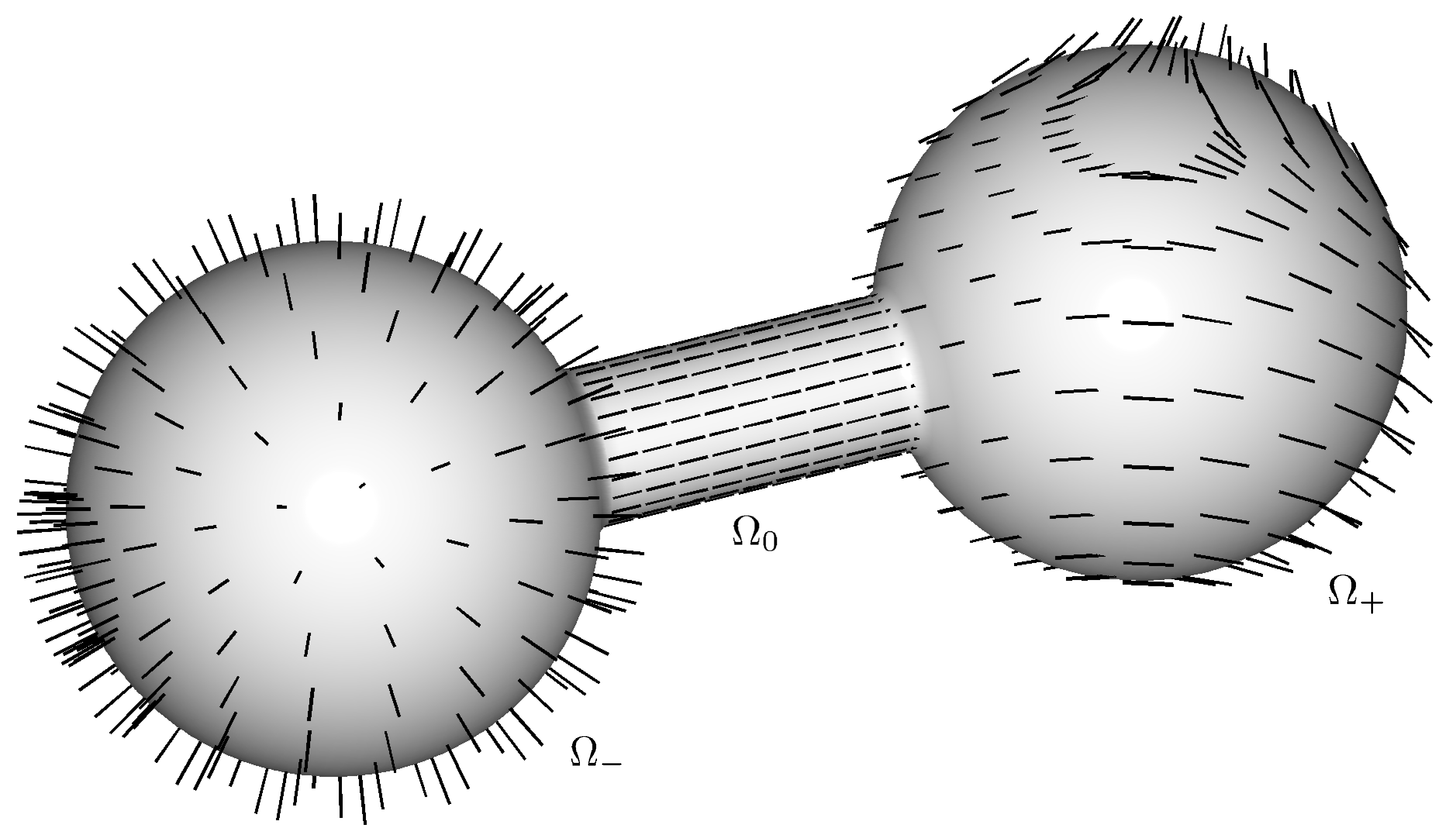
Figure 1: The domain considered in Section 7: two unit balls ($\Omega_{-}$ on the left, $\Omega_{+}$ on the right) joined by a cylinder $\Omega_{0}$ of length $2L$ and radius $r$. The (unoriented) director field associated to the boundary datum is also represented. The boundary datum restricted to the boundary of $\Omega_{-}$, $\Omega_{+}$ defines non-trivial homotopy classes in $\pi_{2}(\mathscr{N})$, $\pi_{1}(\mathscr{N})$ respectively.

Finally, we consider an example where both $\mathscr{S}_{\mathrm{line}}$ and $\mathscr{S}_{\mathrm{pts}}$ are non-empty. The domain consists of two balls of radius $1$, joined by a cylinder of radius $r\in(0,\,1/2)$ and length $2L$. The boundary datum, which is defined in Section 7, is uniaxial and has two point defects. In Figure 1, we represent the behaviour of the boundary datum or, more precisely, the direction of the eigenspace corresponding to the leading eigenvalue (that is, the average orientation of the molecules at each point). This map defines non-trivial homotopy classes both in $\pi_{1}(\mathscr{N})$ and in $\pi_{2}(\mathscr{N})$.

Proposition 6.

There exists a positive number $L^{*}$ such that, if $L\geq L^{*}$, then $\mathscr{S}_{\mathrm{line}}$ is non-empty and there exists a point $x_{0}\in\mathscr{S}_{\mathrm{pts}}$ such that $\operatorname{dist}(x_{0},\,\mathscr{S}_{\mathrm{line}})\geq L/2$.

In other words, if the cylinder is long enough then the limit configuration has line defects and at least one point defect, which is far from the line defects. Although the boundary datum defines a non-trivial class in $\pi_{2}(\mathscr{N})$, topological arguments alone are not enough to conclude that $\mathscr{S}_{\mathrm{pts}}\neq\emptyset$, for there exist maps $\Omega\to\mathscr{N}$ which satisfy the boundary condition and $\mathscr{S}_{\mathrm{line}}\neq\emptyset$, $\mathscr{S}_{\mathrm{pts}}=\emptyset$ (see Remark 7.1). Proposition 6 is inspired by Hardt and Lin’s paper [38], where the existence of minimizing harmonic maps with non-topologically induced singularities is proved. However, there is an additional difficulty here, namely minimizers are not uniformly bounded in $H^{1}$ as $\varepsilon\to 0$. We take care of this issue by adapting some ideas of the proof of Theorem 1.

Let us spend a few word on the proof of our main result, Theorem 1. The core of the argument is a concentration property for the energy, which can be stated as follows.

Proposition 7.

Assume that the condition (H) holds. For any $0<\theta<1$ there exist positive numbers $\eta$, $\epsilon_{0}$ and $C$ such that, for any $x_{0}\in\Omega$, $R>0$ satisfying $\overline{B}_{R}(x_{0})\subseteq\Omega$ and any $0<\varepsilon\leq\epsilon_{0}R$, if

(10) $$E_{\varepsilon}(Q_{\varepsilon},\,B_{R}(x_{0}))\leq\eta R\log\frac{R}{\varepsilon}$$

then

$$E_{\varepsilon}(Q_{\varepsilon},\,B_{\theta R}(x_{0}))\leq CR.$$

Proposition 7 implies that either the energy on a ball blows up at least logarithmically, or it is bounded on a smaller ball. Combining this fact with covering arguments, one proves that the energy concentrates on a set $\mathscr{S}_{\mathrm{line}}$ of finite length. Then, the asymptotic behaviour of minimizers away from $\mathscr{S}_{\mathrm{line}}$ can be studied using well-established techniques, e.g. arguing as in [52].

Roughly speaking, the proof of Proposition 7 goes as follows. Condition (10) implies that the problem can be reformulated in terms of $\mathscr{N}$-valued maps. Indeed, by an average argument we find $r\in(\theta R,\,R)$ such that the energy of $Q_{\varepsilon}$ on the sphere of radius $r$ is controlled by $C\eta|\log\varepsilon|$. On the other hand, the energy per unit length associated with a topological defect line is of the order of $\kappa_{*}|\log\varepsilon|$ (see the estimates by Jerrard and Sandier [43, 59]). Therefore, if $\eta$ is small compared to $\kappa_{*}$, the sphere of radius $r$ intersects no topological defect line of $Q_{\varepsilon}$. This makes it possible to approximate $Q_{\varepsilon}$ with an $\mathscr{N}$-valued map $P_{\varepsilon}$, defined on a sphere of radius $r^{\prime}$ close to $r$. Now, since the sphere is simply connected, $P_{\varepsilon}$ can be lifted to a $\mathbb{S}^{2}$-valued map, i.e. one can write

$$P_{\varepsilon}(x)=s_{*}\left(\mathbf{n}_{\varepsilon}^{\otimes 2}(x)-\frac{1}{3}\operatorname{Id}\right)\qquad\textrm{for }x\in\partial B_{r^{\prime}}(x_{0})$$

for a smooth vector field $\mathbf{n}_{\varepsilon}\colon\partial B_{r^{\prime}}(x_{0})\to\mathbb{S}^{2}$. Thus, we have reduced to a problem which is formulated in terms of vector fields, and we can apply the methods by Hardt, Kinderlehrer and Lin [37, Lemma 2.3] to obtain boundedness of the energy. In other words, Condition (10) enable us to reduce the asymptotic analysis of the Landau-de Gennes problem to the analysis of the Oseen-Frank problem. Extension results are needed in several steps of this proof, for instance to interpolate between $Q_{\varepsilon}$ and $P_{\varepsilon}$ in order to construct an admissible comparison map. Various results in this direction are discussed in detail in Section 3. In particular, we prove variants of Luckhaus’ lemma [49, Lemma 1] which are fit for our purposes.

Remark 2.

Condition (H) is not sufficient to obtain compactness for minimizers of the Ginzburg-Landau energy. Indeed, Brezis and Mironescu [18] constructed a sequence of minimizers $u_{\varepsilon}\in H^{1}(B^{2}_{1},\,\mathbb{C})$ such that

$$E^{\mathrm{GL}}_{\varepsilon}(u_{\varepsilon},\,B_{1}^{2})\ll\left|\log\varepsilon\right|\qquad\textrm{and}\qquad\left|u_{\varepsilon}\right|\leq 1,$$

yet $\{u_{\varepsilon}\}_{0<\varepsilon<1}$ does not have subsequences converging a.e. on sets of positive measure. Brezis and Mironescu’s example relies on oscillations of the phase. Indeed, the $u_{\varepsilon}$’s can be lifted to $\mathbb{R}$-valued functions $\varphi_{\varepsilon}$’s (that is $u_{\varepsilon}\approx\exp(i\varphi_{\varepsilon})$), but the latter are not uniformly bounded in $L^{\infty}$. This phenomenon does not occur in our case, because the $\mathscr{N}$-valued map $P_{\varepsilon}$ is lifted to a unit vector field. The finiteness of the fundamental group $\pi_{1}(\mathscr{N})$ yields the compactness of the universal covering of $\mathscr{N}$, hence better compactness properties for the minimizers.

1.4 Concluding remarks and open questions

Several questions about minimizers of the Landau-de Gennes functional on three-dimensional domains remain open. A first question concerns the behaviour of the singular set $\mathscr{S}_{\mathrm{line}}$. Since $\mathscr{S}_{\mathrm{line}}$ is obtained as a limit of minimizers, one would expect that it inherits from $Q_{\varepsilon}$ minimizing properties. It is natural to conjecture that $\mathscr{S}_{\mathrm{line}}$ is a relative cycle, whose homology class is determined by the domain and the boundary datum, and that $\mathscr{S}_{\mathrm{line}}$ has minimal length in its homology class. For instance, if the domain is convex and the boundary data has a finite number of point singularities $x_{1},\,\ldots,\,x_{p}$ of the form (8), then $\mathscr{S}_{\mathrm{line}}$ should be a union of non-intersecting straight lines connecting the $x_{i}$’s in pairs, in such a way that the total length of $\mathscr{S}_{\mathrm{line}}$ is minimal. (Notice that, by topological arguments, the number $p$ must be even.) However, if the domain is non-convex, then a part of $\mathscr{S}_{\mathrm{line}}$ may lie on the boundary.

It would be interesting to study the structure of minimizers $Q_{\varepsilon}$ in the core of line defects. For instance, does the core of line defects contain biaxial phases? Contreras and Lamy [25] and Majumdar, Pisante and Henao [51] proved that the core of point singularities, in dimension three, contains biaxial phases when the temperature is low enough. Their proofs use a uniform energy bound such as (5), so they do not apply directly to singularities of codimension two. However, the analysis of point defects on two-dimensional domains (see e.g. [21, 28, 42]) suggests that line defects may also contain biaxial phases, when the temperature is low. A related issue is the analysis of singularity profiles. Let $x_{0}\in\mathscr{S}_{\mathrm{line}}$ and let $\Pi$ be an orthogonal plane to $\mathscr{S}_{\mathrm{line}}$, passing through the point $x_{0}$. Set

$$P_{\varepsilon,x_{0}}(y):=Q_{\varepsilon}(x_{0}+\varepsilon y)\qquad\textrm{for }y\in\Pi.$$

This defines a bounded sequence in $L^{\infty}(\Pi,\,\mathbf{S}_{0})$, such that

$$\left\|\nabla P_{\varepsilon,x_{0}}\right\|_{L^{2}(K)}=\left\|\nabla Q_{\varepsilon}\right\|_{L^{2}(x_{0}+\varepsilon K)}\leq C(K)\qquad\textrm{for every }K\subset\!\subset\Pi.$$

Therefore, up to a subsequence we have $P_{\varepsilon,x_{0}}\rightharpoonup P_{x_{0}}$ in $H^{1}_{\mathrm{loc}}(\Pi,\,\mathbf{S}_{0})$. The map $P_{x_{0}}$ contains the information on the fine structure of the defect core. What can be said about $P_{x_{0}}$?

In another direction, investigating the asymptotic behaviour of a more general class of functionals in the logarithmic energy regime is a challenging issue. For instance, one may consider functionals with more elastic energy terms and/or choose different potentials, such as the sextic potential

$$f(Q):=-\frac{a_{1}}{2}\operatorname{tr}Q^{2}-\frac{a_{2}}{3}\operatorname{tr}Q^{3}+\frac{a_{3}}{4}\left(\operatorname{tr}Q^{2}\right)^{2}+\frac{a_{4}}{5}\left(\operatorname{tr}Q^{2}\right)\left(\operatorname{tr}Q^{3}\right)+\frac{a_{5}}{6}\left(\operatorname{tr}Q^{2}\right)^{3}+\frac{a_{5}^{\prime}}{6}\left(\operatorname{tr}Q^{3}\right)^{2}$$

(see [26, 36]) or the singular potential proposed by Ball and Majumdar [8]. From this point of view, it is interesting to remark that the proof of Proposition 7 is quite robust, as it is based on variational arguments alone and does not use the structure of the Euler-Lagrange system. Therefore, the proof of Proposition 7 could be adapted to other choices of the elastic energy density, provided that they are quadratic in the gradient, and other potentials $f$, possibly infinite-valued outside some convex set, provided that they satisfy some non-degeneracy conditions around their set of minimizers (see Lemma 2.4). This would yield local $H^{1}$-compactness, away from a singular set of dimension one, for minimizers of more general Landau-de Gennes functionals. However, proving stronger compactness for minimizers (e.g., with respect to the uniform norm) and understanding the structure of the singular set $\mathscr{S}_{\mathrm{line}}$ for the general Landau-de Gennes energy are completely open questions.

The paper is organized as follows. Section 2 deals with general facts about the space of $Q$-tensors and Landau-de Gennes minimizers. In particular, lower estimates for the energy of $Q$-tensor valued maps are established in Subsection 2.2, by adapting Jerrard’s and Sandier’s arguments. Section 3 contains several extension results, which are a fundamental tool for the proof of our main theorem. Section 4 aims at proving Theorem 1, and in particular it contains the proof of Proposition 7 (Section 4.1). The asymptotic analysis away from the singular lines is carried out in Section 4.2, whereas the singular set $\mathscr{S}_{\mathrm{line}}$ is defined and studied in Section 4.3. In Section 4.4, we work out the analysis of minimizers near the boundary of the domain. Section 5 deals with the proof of Proposition 2. We first show the stationarity of $\mu_{0}$ (Section 5.1); then, with the help of an auxiliary problem (Section 5.2), we compute the density of $\mu_{0}$ and conclude the proof (Section 5.3). In Section 5.4, we construct an example where $\mu_{0}$ concentrates at the boundary of the domain. Section 6 deals with the proofs of Propositions 3 (Section 6.1), 4 and 5 (Section 6.2). Finally, in Section 7 we prove Proposition 6 by constructing an example where the limit configuration $Q_{0}$ has both lines and point singularities.

2 Preliminary results

Throughout the paper, we use the following notation. We denote by $B^{k}_{r}(x)$ (or, occasionally, $B^{k}(x,\,r)$) the $k$-dimensional open ball of radius $r$ and center $x$, and by $\overline{B}^{k}_{r}(x)$ the corresponding closed ball. When $k=3$, we omit the superscript and write $B_{r}(x)$ instead of $B_{r}^{3}(x)$. When $x=0$, we write $B_{r}^{k}$ or $B_{r}$. Balls in the matrix space $\mathbf{S}_{0}$ will be denoted $B^{\mathbf{S}_{0}}_{r}(Q)$ or $B^{\mathbf{S}_{0}}_{r}$. For any $Q\in H^{1}(\Omega,\,\mathbf{S}_{0})$ and any $k$-submanifold $U\subseteq\Omega$, we set

$$e_{\varepsilon}(Q):=\frac{1}{2}\left|\nabla Q\right|^{2}+\frac{1}{\varepsilon^{2}}f(Q),\qquad E_{\varepsilon}(Q,\,U):=\int_{U}e_{\varepsilon}(Q)\,\mathrm{d}\mathscr{H}^{k}.$$

The function $e_{\varepsilon}(Q)$ will be called the energy density of $Q$. We also set $E_{\varepsilon}(Q,\,\emptyset):=0$ for any map $Q$. Additional notation will be set later on.

2.1 Properties of $\mathbf{S}_{0}$ and $f$

We discuss general facts about $Q$-tensors, which are useful in order to to have an insight into the structure of the target space $\mathbf{S}_{0}$. The starting point of our analysis is the following representation formula.

Lemma 2.1.

For all fixed $Q\in\mathbf{S}_{0}\setminus\{0\}$, there exist two numbers $s\in(0,\,+\infty)$, $r\in[0,\,1]$ and an orthonormal pair of vectors $(\mathbf{n},\,\mathbf{m})$ in $\mathbb{R}^{3}$ such that

$$Q=s\left\{\mathbf{n}^{\otimes 2}-\frac{1}{3}\operatorname{Id}+r\left(\mathbf{m}^{\otimes 2}-\frac{1}{3}\operatorname{Id}\right)\right\}.$$

Given $Q$, the parameters $s=s(Q)$, $r=r(Q)$ are uniquely determined. The functions $Q\mapsto s(Q)$ and $Q\mapsto r(Q)$ are continuous on $\mathbf{S}_{0}\setminus\{0\}$, and are positively homogeneous of degree $1$ and $0$, respectively.

Slightly different forms of this formula are often found in the literature (e.g. [52, Proposition 1]). The proof is a straightforward computation sketched in [21, Lemma 3.2], so we omit it here.

Remark 2.1.

The parameters $s(Q)$, $r(Q)$ are determined by the eigenvalues $\lambda_{1}(Q)\geq\lambda_{2}(Q)\geq\lambda_{3}(Q)$ according to this formula:

$$s(Q)=2\lambda_{1}(Q)+\lambda_{2}(Q),\qquad r(Q)=\frac{\lambda_{1}(Q)+2\lambda_{2}(Q)}{2\lambda_{1}(Q)+\lambda_{2}(Q)}.$$

Following [52, Proposition 15], the vacuum manifold $\mathscr{N}:=f^{-1}(0)$ can be characterized as follows:

(2.1) $$Q\in\mathscr{N}\qquad\textrm{if and only if }s(Q)=s_{*}\textrm{ and }r(Q)=0,$$

where

$$s_{*}:=\frac{1}{4c}\left(b+\sqrt{b^{2}+24ac}\right).$$

There is another set which is important for our analysis, namely

$$\mathscr{C}:=\bigg{\{}Q\in\mathbf{S}_{0}\colon\lambda_{1}(Q)=\lambda_{2}(Q)\bigg{\}},$$

i.e. $\mathscr{C}$ is the set of matrices whose leading eigenvalue has multiplicity $>1$. This is a closed subset of $\mathscr{C}$, and it is cone (i.e., $\mu Q\in\mathscr{C}$ for any $Q\in\mathscr{C}$, $\mu\in\mathbb{R}^{+}$). By Remark 2.1, we see that

$$Q\in\mathscr{C}\qquad\textrm{if and only if }s(Q)=0\textrm{ or }r(Q)=1.$$

Then, applying Lemma 2.1 and the identity $\operatorname{Id}=\mathbf{n}^{\otimes 2}+\mathbf{m}^{\otimes 2}+\mathbf{p}^{\otimes 2}$ (where $(\mathbf{n},\,\mathbf{m},\,\mathbf{p})$ is any orthonormal, positive basis of $\mathbb{R}^{3}$), we see that $Q\in\mathscr{C}$ if and only if there exist $s\geq 0$ and $\mathbf{p}\in\mathbb{S}^{2}$ such that

(2.2) $$Q=-s\left(\mathbf{p}^{\otimes 2}-\frac{1}{3}\operatorname{Id}\right).$$

Therefore, $\mathscr{C}$ is the cone over the projective plane $\mathbb{RP}^{2}$. The importance of $\mathscr{C}$ is explained by the following fact. Away from $\mathscr{C}$, it is possible to define locally a continuous map $Q\mapsto\mathbf{n}(Q)$, which selects a unit eigenvector $\mathbf{n}(Q)$ associated with $\lambda_{1}(Q)$ (see e.g. [7, Section 9.1, Equation (9.1.41)]). In particular, the map $\varrho\colon\mathbf{S}_{0}\setminus\mathscr{C}\to\mathscr{N}$ defined by

(2.3) $$\varrho(Q):=s_{*}\left(\mathbf{n}(Q)-\frac{1}{3}\operatorname{Id}\right)\qquad\textrm{for }Q\in\mathbf{S}_{0}\setminus\mathscr{C}$$

is continuous. It was proven in [21, Lemma 3.10] that $\varrho$ gives a retraction by deformation of $\mathbf{S}_{0}\setminus\mathscr{C}$ onto the vacuum manifold $\mathscr{N}$.

Lemma 2.2.

The retraction $\varrho$ is of class $C^{1}$ on $\mathbf{S}_{0}\setminus\mathscr{C}$. Moreover, $\varrho$ coincides with the nearest-point projection onto $\mathscr{N}$, that is

(2.4) $$\left|Q-\varrho(Q)\right|\leq\left|Q-P\right|$$

holds for any $Q\in\mathbf{S}_{0}\setminus\mathscr{C}$ and any $P\in\mathscr{N}$, with strict inequality if $P\neq\varrho(Q)$.

Proof.

Fix a matrix $Q_{0}\in\mathbf{S}_{0}\setminus\mathscr{C}$. By definition of $\mathscr{C}$, the leading eigenvalue $\lambda_{1}(Q)$ is simple. Then, classical differentiability results for the eigenvectors (see e.g. [7, Section 9.1]) imply that the map $Q\mapsto\mathbf{n}(Q)$ which appears in (2.3) is locally of class $C^{1}$, in a neighborhood of $Q_{0}$. As a consequence, $\varrho$ is of class $C^{1}$ in a neighborhood of $Q_{0}$, and since $Q_{0}$ is arbitrary we have $\varrho\in C^{1}(\mathbf{S}_{0}\setminus\mathscr{C})$.

To show that $\varrho$ is the nearest point projection onto $\mathscr{N}$, we pick an arbitrary $Q\in\mathbf{S}_{0}\setminus\mathscr{C}$ and $P\in\mathscr{N}$. By applying Lemma 2.1 and (2.1), we write

$$Q=s\left(\mathbf{n}^{\otimes 2}-\frac{1}{3}\operatorname{Id}\right)+sr\left(\mathbf{m}^{\otimes 2}-\frac{1}{3}\operatorname{Id}\right)\qquad\textrm{and}\qquad P=s_{*}\left(\mathbf{p}^{\otimes 2}-\frac{1}{3}\operatorname{Id}\right)$$

for some numbers $s>0$ and $0\leq r<1$, some orthonormal pair $(\mathbf{n},\,\mathbf{m})$ and some unit vector $\mathbf{p}$. We compute that

$$\begin{split}\left|Q-P\right|^{2}&=\left|s\mathbf{n}^{\otimes 2}+sr\mathbf{m}^{\otimes 2}-s_{*}\mathbf{p}^{\otimes 2}-\frac{1}{3}(s+sr-s_{*})\operatorname{Id}\right|^{2}\\ &=C(s,\,r,\,s_{*})-2s_{*}s\bigg{\{}(\mathbf{n}\cdot\mathbf{p})^{2}+r(\mathbf{m}\cdot\mathbf{p})^{2}\bigg{\}}\end{split}$$

where $C(s,\,r,\,s_{*})$ is a constant which only depends on $s$, $r$ and $s_{*}$. For the last equality, we have used the identities $\mathbf{u}^{\otimes 2}\cdot\mathbf{v}^{\otimes 2}=(\mathbf{u}\cdot\mathbf{v})^{2}$ and $\mathbf{u}^{\otimes 2}\cdot\operatorname{Id}=|\mathbf{u}|^{2}$, which hold for any vectors $\mathbf{u}$, $\mathbf{v}$. Given $s$, $r$, $\mathbf{n}$ and $\mathbf{m}$, we minimize the right-hand side with respect to $\mathbf{p}$, subject to the constraint

$$(\mathbf{n}\cdot\mathbf{p})^{2}+(\mathbf{m}\cdot\mathbf{p})^{2}\leq 1.$$

Since $r<1$, one easily sees that the minimum is achieved if and only if $\mathbf{p}=\pm\mathbf{n}$, that is $P=\varrho(Q)$. ∎

Another function will be involved in the analysis of Section 2.2. Let $\phi\colon\mathbf{S}_{0}\to\mathbb{R}$ be given by

(2.5) $$\phi(Q)=s_{*}^{-1}\left(\lambda_{1}(Q)-\lambda_{2}(Q)\right),$$

where $\lambda_{1}(Q)$ and $\lambda_{2}(Q)$ are the largest and the second-largest eigenvalue of $Q$. It is clear that $\phi\geq 0$, and $\phi(Q)=0$ if and only if $Q\in\mathscr{C}$. Moreover, by applying Remark 2.1 we have

$$\phi(Q):=s_{*}^{-1}s(Q)(1-r(Q))\qquad\textrm{for any }Q\in\mathbf{S}_{0}\setminus\{0\},$$

therefore we have $\phi(Q)=1$ if $Q\in\mathscr{N}$, thanks to (2.1).

Lemma 2.3.

The function $\phi$ is Lipschitz continuous on $\mathbf{S}_{0}$, of class $C^{1}$ on $\mathbf{S}_{0}\setminus\mathscr{C}$ and satisfies

$$\sqrt{2}s_{*}^{-1}\leq\left|\mathrm{D}\phi(Q)\right|\leq 2s_{*}^{-1}\qquad\textrm{for any }Q\in\mathbf{S}_{0}\setminus\mathscr{C}.$$

Proof.

Thanks to standard regularity results for the eigenvalues (see e.g. [7, Equation (9.1.32)]), we immediately deduce that $\phi$ is locally Lipschitz continuous on $\mathbf{S}_{0}$ and of class $C^{1}$ on $\mathbf{S}_{0}\setminus\mathscr{C}$. Let $(\mathbf{n},\,\mathbf{m},\,\mathbf{p})$ be an orthonormal set of eigenvectors relative to $(\lambda_{1},\,\lambda_{2},\,\lambda_{3})$ respectively. Then, for any $Q\in\mathbf{S}_{0}\setminus\mathscr{C}$ there holds

$$s_{*}\left|\mathrm{D}\phi(Q)\right|=\max_{B\in\mathbf{S}_{0},\ |B|=1}\left|\frac{\partial\phi}{\partial B}(Q)\right|=\max_{B\in\mathbf{S}_{0},\ |B|=1}\left|\mathbf{n}\cdot B\mathbf{n}-\mathbf{m}\cdot B\mathbf{m}\right|$$

(the last identity follows by differentiating (2.5), with the help of [7, Equation (9.1.32)] again). This implies $\left|\mathrm{D}\phi(Q)\right|\leq 2$. Now, set

$$B_{0}:=\frac{1}{\sqrt{2}}\left(\mathbf{n}^{\otimes 2}-\mathbf{m}^{\otimes 2}\right)\in\mathbf{S}_{0}.$$

Since $|\mathbf{n}^{\otimes 2}|=|\mathbf{m}^{\otimes 2}|=1$ and $\mathbf{n}^{\otimes 2}\cdot\mathbf{m}^{\otimes 2}=0$, it is straightforward to check that $|B_{0}|=1$, so

$$s_{*}\left|\mathrm{D}\phi(Q)\right|\geq\left|\mathbf{n}\cdot B_{0}\mathbf{n}-\mathbf{m}\cdot B_{0}\mathbf{m}\right|=\frac{1}{\sqrt{2}}\left(|\mathbf{n}|^{2}+|\mathbf{m}|^{2}\right)=\sqrt{2}.\qed$$

We conclude our discussion on the structure of the target space $\mathbf{S}_{0}$ by proving a couple of properties of the Landau-de Gennes potential $f$, defined by (3).

Lemma 2.4.

There exists a constant $\gamma=\gamma(a,\,b,\,c)>0$ with the following properties. For any $Q\in\mathbf{S}_{0}$, there holds

(F₀) $$f(Q)\geq\gamma\left(1-\phi(Q)\right)^{2}.$$

For any $Q_{0}\in\mathscr{N}$ and any matrix $P\in\mathbf{S}_{0}$ which is orthogonal to $T_{Q_{0}}\mathscr{N}$, we have

(F₁) $$\frac{\mathrm{d}^{2}}{\mathrm{d}t^{2}}_{|t=0}\,f(Q_{0}+tP)\geq\gamma|P|^{2}.$$

As a consequence of (F₁), there exist $\gamma^{\prime}$ and $\delta_{0}>0$ such that, if $Q\in\mathbf{S}_{0}$ satisfies $\operatorname{dist}(Q,\,\mathscr{N})\leq\delta_{0}$, then

(F₂) $$f(Q)\geq\gamma^{\prime}\operatorname{dist}^{2}(Q,\,\mathscr{N})$$

and

(F₃) $$f\left(tQ+(1-t)\varrho(Q)\right)\leq\gamma^{\prime}t^{2}f(Q)$$

for any $0\leq t\leq 1$.

Proof of (F₀).

Using the representation formula of Lemma 2.1, we can compute $\operatorname{tr}Q^{2}$ and $\operatorname{tr}Q^{3}$ as functions of $s:=s(Q)$, $t:=s(Q)r(Q)$. This yields

$$f(Q)=k-\frac{a}{3}\left(s^{2}-st+t^{2}\right)-\frac{b}{27}\left(2s^{3}-3s^{2}t+3st^{2}-2t^{3}\right)+\frac{c}{9}\left(s^{2}-st+t^{2}\right)^{2}=:\tilde{f}(s,\,t).$$

We know that $(s_{*},\,0)$ is the unique minimizer of $\tilde{f}$ (see e.g. [52, Proposition 15]), so $\mathrm{D}^{2}\tilde{f}(s_{*},\,0)\geq 0$. Moreover, it is straightforward to compute that

$$\begin{split}\det\mathrm{D}^{2}\tilde{f}(s_{*},\,0)>0\end{split}$$

thus $\mathrm{D}^{2}\tilde{f}(s_{*},\,0)>0$. As a consequence, there exist two numbers $\delta>0$ and $C>0$ such that

(2.6) $$\tilde{f}(s,\,sr)\geq C(s_{*}-s)^{2}+Cs^{2}r^{2}\qquad\textrm{if }(s-s_{*})^{2}+s^{2}r^{2}\leq\delta.$$

The left-hand side in this inequality is a polynomial of order four with leading term $\frac{c}{9}(s^{2}-st+t^{2})^{2}\geq\frac{c}{36}(s^{2}+t^{2})^{2}$, whereas the right-hand side is a polynomial of order two. Therefore, there exists a positive number $M$ such that

(2.7) $$\tilde{f}(s,\,sr)\geq C(s_{*}-s)^{2}+Cs^{2}r^{2}\qquad\textrm{if }(s-s_{*})^{2}+s^{2}r^{2}\geq M.$$

Finally, we have $\tilde{f}(s,\,t)>0$ for any $(s,\,t)\neq(s_{*},\,0)$, so there exists a positive constant $C^{\prime}$ such that

(2.8) $$\tilde{f}(s,\,sr)\geq C^{\prime}\qquad\textrm{if }\delta<(s-s_{*})^{2}+s^{2}r^{2}\leq M.$$

Combining (2.6), (2.7) and (2.8), and modifying the value of $C$ if necessary, for any $Q\in\mathbf{S}_{0}$, $s=s(Q)$, $r=r(Q)$ we obtain

$$\begin{split}\tilde{f}(s,\,sr)\geq C(s_{*}-s)^{2}+Cs^{2}r^{2}\geq\frac{Cs_{*}^{2}}{2}\left(1-\frac{s}{s_{*}}+\frac{sr}{s_{*}}\right)^{2}=\frac{Cs_{*}^{2}}{2}\left(1-\phi(Q)\right)^{2}.\qed\end{split}$$

Proof of (F₁).

Since the group $\mathrm{SO}(3)$ acts transitively on the manifold $\mathscr{N}$ and the potential $f$ is preserved by the action, it suffices to check (F₁) in case

(2.9) $$Q_{0}=s_{*}\left(\mathbf{e}^{\otimes 2}-\frac{1}{3}\operatorname{Id}\right).$$

Indeed, for any $Q\in\mathbf{S}_{0}$ there exists $\mathbf{n}\in\mathbb{S}^{2}$ such that

$$\varrho(Q)=s_{*}\left(\mathbf{n}^{\otimes 2}-\frac{1}{3}\operatorname{Id}\right),$$

and there exists a matrix $R\in\mathrm{SO}(3)$ such that $R\mathbf{n}=\mathbf{e}_{3}$. As is easily checked, the function $\xi_{R}\colon Q\mapsto RQR^{\mathsf{T}}$ maps isometrically $\mathbf{S}_{0}$ onto itself. Then, (2.4) implies that $\xi_{R}$ commutes with $\varrho$, so

$$\varrho(\xi_{R}(Q))=\xi_{R}(\varrho(Q))=s_{*}\left(R\mathbf{n}(R\mathbf{n})^{\mathsf{T}}-\frac{1}{3}\operatorname{Id}\right)=s_{*}\left(\mathbf{e}_{3}\mathbf{e}_{3}^{\mathsf{T}}-\frac{1}{3}\operatorname{Id}\right).$$

On the other hand, $f$ is invariant by composition with $\xi_{R}$ (i.e. $f\circ\xi_{R}=f$) because it is a function of the scalar invariants of $Q$. Therefore, we assume WLOG that $Q_{0}$ is given by (2.9).

In [21, Lemma 3.5], it is shown that a matrix $P\in\mathbf{S}_{0}$ is orthogonal to $T_{{Q}_{0}}\mathscr{N}$ if and only if it can be written in the form

$$P=\left(\begin{matrix}-\dfrac{1}{3}(s_{*}+x_{0})+x_{2}&x_{1}&0\\ x_{1}&-\dfrac{1}{3}(s_{*}+x_{0})-x_{2}&0\\ 0&0&\dfrac{2}{3}(s_{*}+x_{0})\end{matrix}\right)$$

for some $x=(x_{0},\,x_{1},\,x_{2})\in\mathbb{R}^{3}$. Then, one can write $f(Q_{0}+tP)$ as a function of $t$, $x$ and compute the second derivatives. The proof of (F₁) is reduced to a straightforward computation, which we omit here. ∎

Proof of (F₂)–(F₃).

These properties follow from (F₁), by a Taylor expansion of $f$ around $Q_{0}$. ∎

2.2 Energy estimates in $2$-dimensional domains

In the analysis of the Ginzburg-Landau functional, a very useful tool are the estimates proved by Jerrard [43] and Sandier [59]. These estimates provide a lower bound for the energy of complex-valued maps defined on a two-dimensional disk, depending on the topological properties of the boundary datum. More precisely, if $u\in H^{1}(B^{2}_{1},\,\mathbb{C})$ satisfies $|u(x)|=1$ for a.e. $x\in\partial B^{2}_{1}$ (plus some technical assumptions) then

(2.10) $$E^{\mathrm{GL}}_{\varepsilon}(u,\,B^{2}_{1})\geq\pi\left|d\right|\left|\log\varepsilon\right|-C,$$

where $E^{\mathrm{GL}}_{\varepsilon}$ is the Ginzburg-Landau energy, defined by (7), and $d$ denotes the topological degree of $u/|u|$ on $\partial B^{2}_{1}$, i.e. its winding number. The aim of this subsection is to generalize this result to tensor-valued maps and the Landau-de Gennes energy.

Since we work in the $H^{1}$-setting, we have to take care of a technical detail. Set $A:=B^{2}_{1}\setminus B^{2}_{1/2}$. Let $Q\in H^{1}(B^{2}_{1},\,\mathbf{S}_{0})$ be a given map, which satisfies

(2.11) $$\phi_{0}(Q,\,A):=\underset{A}{\operatorname{ess\,inf}}\,\phi\circ Q>0.$$

In case $Q$ is continuous, Condition (2.11) is equivalent to

$$Q(x)\notin\mathscr{C}\qquad\textrm{for every }x\in\overline{A}.$$

For a.e. $r\in(1/2,\,1)$ the restriction of $Q$ to $\partial B^{2}_{r}$ is an $H^{1}$-map (due to Fubini theorem) and hence, by Sobolev injection, it is a continuous map which satisfies $Q(x)\notin\mathscr{C}$ for every $x\in\partial B^{2}_{r}$. Therefore, $\varrho\circ Q$ is well defined and continuous on $\partial B^{2}_{r}$. Moreover, its homotopy class is independent of $r$. If $\varrho\circ Q$ is continuous, then $\varrho\circ Q$ itself provides a homotopy between $\varrho\circ Q_{|\partial B^{2}_{r_{1}}}$ and $\varrho\circ Q_{|\partial B^{2}_{r_{2}}}$, for any $r_{1}$ and $r_{2}$. Otherwise, by convolution (as in [61, Proposition p. 267]) one constructs a smooth approximation $(\varrho\circ Q)_{\delta}\colon A\to\mathscr{N}$ such that $(\varrho\circ Q)_{\delta}\to\varrho\circ Q$ in $H^{1}(A,\,\mathbf{S}_{0})$ when $\delta\to 0$. By Fubini theorem and Sobolev injection, we have $(\varrho\circ Q)_{\delta}\to\varrho\circ Q$ uniformly on $\partial B^{2}_{r}$ for a.e. $r\in(1/2,\,1)$. Therefore, the maps $\varrho\circ Q_{|\partial B^{2}_{r}}$ belong to the same homotopy class, for a.e. $r$. By abuse of notation, this homotopy class will be called “homotopy class of $\varrho\circ Q$ restricted to the boundary” or also “homotopy class of the boundary datum”.

Proposition 2.5.

There exist positive constants $M$ and $\kappa_{*}$, depending only on $f$, with the following property. Let $0<\varepsilon<1$ and $Q\in H^{1}(B^{2}_{1},\,\mathbf{S}_{0})$ be given. Assume that $Q$ satisfies (2.11) and the homotopy class of $\varrho\circ Q_{|\partial B^{2}_{1}}$ is non-trivial. Then

$$E_{\varepsilon}(Q,\,B_{1}^{2})\geq\kappa_{*}\phi_{0}^{2}(Q,\,A)\left|\log\varepsilon\right|-M.$$

The energetic cost associated with topological defects is quantified by a number $\kappa_{*}$, defined by (2.16) and explicitly computed in Lemma 2.9:

$$\kappa_{*}=\frac{\pi}{2}s_{*}^{2}.$$

This number plays the same role as the quantity $\pi|d|$ in (2.10). The quantity $\phi_{0}^{2}(Q,\,A)$ at the right-hand side has been introduced for technical reasons. Notice that $\phi=1$ on $\mathscr{N}$, so $\phi_{0}(Q,\,A)=1$ if $Q_{|A}$ takes values in $\mathscr{N}$.

Before dealing with the proof of Proposition 2.5, we state an immediate consequence.

Corollary 2.6.

Let $\varepsilon$, $R$ be two numbers such that $0<\varepsilon<R/2$. Given a map $Q\in H^{1}(B^{2}_{R},\,\mathbf{S}_{0})$, suppose that the restriction to the boundary belongs to $H^{1}(\partial B^{2}_{R},\,\mathbf{S}_{0})$ and that

$$\phi_{0}(Q,\,\partial B^{2}_{R}):=\underset{\partial B^{2}_{R}}{\operatorname{ess\,inf}}\,\phi\circ Q>0.$$

If the homotopy class of $\varrho\circ{Q}_{|\partial B^{2}_{R}}$ is non-trivial, then

$$E_{\varepsilon}(Q,\,B_{R}^{2})+(\log 2)R\,E_{\varepsilon}(Q,\,\partial B_{R}^{2})\geq\kappa_{*}\phi_{0}^{2}(Q,\,\partial B^{2}_{R})\log\frac{R}{\varepsilon}-M.$$

In particular, if $Q$ satisfies $Q=g$ on $\partial B^{2}_{R}$ for some non-trivial $g\in H^{1}(\partial B^{2}_{R},\,\mathscr{N})$, then Corollary 2.6 implies

$$E_{\varepsilon}(Q,\,B_{R}^{2})\geq\kappa_{*}\log\frac{R}{\varepsilon}-M$$

for a constant $M=M(R,\,g)$. (Compare this estimate with [43, Theorem 3.1], [59, Theorem 1], and [23, Proposition 6.1].)

Proof of Corollary 2.6.

We apply Proposition 2.5 to $\epsilon:=2\varepsilon/R$ and the map $\tilde{Q}\in H^{1}(B_{1}^{2},\,\mathbf{S}_{0})$ defined by

$$\tilde{Q}(x):=\begin{cases}Q\left(\dfrac{Rx}{|x|}\right)&\textrm{if }x\in A:=B^{2}_{1}\setminus B^{2}_{1/2}\\ Q\left(2Rx\right)&\textrm{if }x\in B^{2}_{1/2}.\end{cases}$$

Notice that $\phi_{0}(\tilde{Q},\,A)=\phi_{0}(Q,\,\partial B^{2}_{R})$. Then, by a change of variable, we deduce

$$\begin{split}\kappa_{*}\phi^{*}(Q)\log\frac{R}{\varepsilon}-C\leq E_{\epsilon}(\tilde{Q},\,B^{2}_{1})&\leq E_{\epsilon}(Q,\,B^{2}_{1/2})+\int_{1/2}^{1}E_{\epsilon}(\tilde{Q},\,\partial B^{2}_{r})\,\mathrm{d}r\\ &=E_{\varepsilon}(Q,\,B^{2}_{R})+\int_{1/2}^{1}\frac{R}{r}E_{2\varepsilon/r}(Q,\,\partial B^{2}_{R})\,\mathrm{d}r\\ &\leq E_{\varepsilon}(Q,\,B^{2}_{R})+(\log 2)R\,E_{\varepsilon}(Q,\,\partial B^{2}_{R}).\qed\end{split}$$

A generalization of the Jerrard-Sandier estimate (2.10) has already been proved by Chiron, in his PhD thesis [23]. Given a smooth, compact manifold without boundary, Chiron considered maps into the cone over $\mathscr{N}$, that is

$$X_{\mathscr{N}}:=\left((0,\,+\infty)\times\mathscr{N}\right)\cup\{0\}\ni u=\left(|u|,\,u/|u|\right)$$

(with a metric defined accordingly). He obtained an estimate analogous to (2.10). In case $\mathscr{N}=\mathbb{S}^{1}$, one has $X_{\mathbb{S}^{1}}\simeq\mathbb{C}$ and the standard estimate (2.10) is recovered. Given a map $u\colon U\subseteq\mathbb{R}^{k}\to X_{\mathscr{N}}$, a key step in Chiron’s arguments is to decompose the gradient of $u$ in terms of modulus and phase, that is

(2.12) $$\left|\nabla u\right|^{2}=\left|\nabla|u|\right|^{2}+\left|u\right|^{2}\left|\nabla\left(u/|u|\right)\right|^{2}\qquad\textrm{a.e. on }U.$$

Chiron’s result does not apply to tensor-valued maps, because the space $\mathbf{S}_{0}$ do not coincide with the cone over $\mathscr{N}$ (the latter only contains uniaxial matrices, whereas $\mathbf{S}_{0}$ also contains biaxial matrices). However, one can prove an estimate in the same spirit as (2.12), namely, the gradient of a map $\Omega\to\mathbf{S}_{0}$ is controlled from below by the gradients of $\phi\circ Q$ and $\varrho\circ Q$.

Lemma 2.7.

Let $U\subseteq\mathbb{R}^{k}$ be a domain and let $Q\in C^{1}(U,\,\mathbf{S}_{0})$. There holds

$$\left|\nabla Q\right|^{2}\geq\frac{s_{*}^{2}}{3}\left|\nabla\left(\phi\circ Q\right)\right|^{2}+\left(\phi\circ Q\right)^{2}\left|\nabla\left(\varrho\circ Q\right)\right|^{2}\qquad\mathscr{H}^{k}\textrm{-a.e. on }U,$$

where we have set $(\phi\circ Q)|\nabla(\varrho\circ Q)|(x):=0$ if $Q(x)\in\mathscr{C}$.

Proof.

First of all, notice that $\varrho\circ Q$ is well-defined on the set where $Q\notin\mathscr{C}$, or equivalently, the set where $\phi\circ Q>0$. Therefore, the right-hand side always makes sense. Because of our choice of the norm, we have

$$\left|\nabla\psi\right|^{2}=\sum_{i=1}^{k}\left|\partial_{x_{i}}\psi\right|^{2}$$

for any scalar or tensor-valued map $\psi$. Thus, it suffices to prove the lemma when $\nabla$ is replaced by the partial derivative operator $\partial_{x_{i}}$, then sum over $i=1,\,\ldots,\,k$. In view of this remark, we assume WLOG that $k=1$.

Since $\phi$ is Lipschitz continuous (Lemma 2.3), we know that $\phi\circ Q\in W^{1,\infty}_{\mathrm{loc}}(U)$. Moreover, $\phi\circ Q=0$ on $Q^{-1}(\mathscr{C})$. Therefore, we have $(\phi\circ Q)^{\prime}=0$ a.e. on $Q^{-1}(\mathscr{C})$ and the lemma is trivially satisfied a.e. on $Q^{-1}(\mathscr{C})$.

For the rest of the proof, we fix a point $x\in U\setminus Q^{-1}(\mathscr{C})$ so that $\phi\circ Q$, $\varrho\circ Q$ are of class $C^{1}$ in a neighborhood of $x$, and the leading eigenvalue of $Q(x)$ has multiplicity one. We are going to distinguish a few cases, depending on whether the others eigenvalues of $Q(x)$ have multiplicity one as well. Suppose first that $r(Q(x))>0$: in this case, all the eigenvalues of $Q(x)$ are simple. Using Lemma 2.1 and the results in [7], the map $Q$ can be locally written as

(2.13) $$Q=s\left(\mathbf{n}^{\otimes 2}-\frac{1}{3}\operatorname{Id}\right)+sr\left(\mathbf{m}^{\otimes 2}-\frac{1}{3}\operatorname{Id}\right),$$

where $s$, $r$, $\mathbf{n}$, $\mathbf{m}$ are $C^{1}$ functions defined in a neighborhood of $x$, satisfying the constraints

$$s>0,\qquad 0<r<1,\qquad\left|\mathbf{n}\right|=\left|\mathbf{m}\right|=1,\qquad\mathbf{n}\cdot\mathbf{m}=0.$$

Then, $\varrho\circ Q$ is of class $C^{1}$ in a neighborhood of $x$, and we can compute $|Q^{\prime}|$, $|(\varrho\circ Q)^{\prime}|$ in terms of $s$, $r$, $\mathbf{n}$, $\mathbf{m}$ and their derivatives. Setting $t:=sr$, a straightforward computation gives

$$s_{*}^{2}{\left(\phi\circ Q\right)^{\prime}}^{2}={s^{\prime}}^{2}-2s^{\prime}t^{\prime}+{t^{\prime}}^{2},\qquad\left|(\varrho\circ Q)^{\prime}\right|^{2}=2s_{*}^{2}\left|\mathbf{n}^{\prime}\right|^{2}$$

and

(2.14) $$\begin{split}\left|Q^{\prime}\right|^{2}&=\frac{2}{3}\left({s^{\prime}}^{2}-s^{\prime}t^{\prime}+{t^{\prime}}^{2}\right)+2s^{2}\left|\mathbf{n}^{\prime}\right|^{2}+2t^{2}\left|\mathbf{m}^{\prime}\right|^{2}+4st(\mathbf{n}^{\prime}\cdot\mathbf{m})(\mathbf{n}\cdot\mathbf{m}^{\prime})\\ &\geq\frac{s_{*}^{2}}{3}{\left(\phi\circ Q\right)^{\prime}}^{2}+2s^{2}\left(\left|\mathbf{n}^{\prime}\right|^{2}+r^{2}\left|\mathbf{m}^{\prime}\right|^{2}+2r(\mathbf{n}^{\prime}\cdot\mathbf{m})(\mathbf{n}\cdot\mathbf{m}^{\prime})\right)\end{split}$$

Let $\mathbf{p}:=\mathbf{n}\times\mathbf{m}$, so that $(\mathbf{n},\,\mathbf{m},\,\mathbf{p})$ is an orthonormal, positive frame in $\mathbb{R}^{3}$. By differentiating the orthogonality conditions for $(\mathbf{n},\,\mathbf{m},\,\mathbf{p})$, we obtain

$$\mathbf{n}^{\prime}=\alpha\mathbf{m}+\beta\mathbf{p},\qquad\mathbf{m}^{\prime}=-\alpha\mathbf{n}+\gamma\mathbf{p}$$

for some smooth, real-valued functions $\alpha$, $\beta$, $\gamma$. Then, from (2.14) and (2.2) we deduce

$$\begin{split}\left|Q^{\prime}\right|^{2}-\frac{s_{*}^{2}}{3}{\left(\phi\circ Q\right)^{\prime}}^{2}&\geq 2s^{2}\left(\alpha^{2}+\beta^{2}+r^{2}(\alpha^{2}+\gamma^{2})-2r\alpha^{2}\right)\\ &\geq 2s^{2}(1-r)^{2}(\alpha^{2}+\beta^{2})\\ &=s_{*}^{-2}{s^{2}(1-r)^{2}}\left|(\varrho\circ Q)^{\prime}\right|^{2}=\left(\phi\circ Q\right)^{2}\left|(\varrho\circ Q)^{\prime}\right|^{2},\end{split}$$

so the lemma holds at the point $x$.

If $r(Q)=0$ in a neighborhood of $x$ then the function $\mathbf{m}$ might not be well-defined. However, the previous computation still make sense because $t=sr$ vanishes in a neighborhood of $x$, and from (2.2), (2.14) we deduce that the lemma holds at $x$. We still have to consider one case, namely, $r(Q(x))=0$ but $r(Q)$ does not vanish identically in a neighborhood of $x$. In this case, there exists a sequence $x_{k}\to x$ such that $r(Q(x_{k}))>0$ for each $k\in\mathbb{N}$. By the previous discussion the lemma holds at each $x_{k}$, and the functions $\phi\circ Q$,  $(\varrho\circ Q)^{\prime}$ are continuous (by Lemmas 2.3 and 2.2). Passing to the limit as $k\to+\infty$, we conclude that the lemma is satisfied at $x$ as well. ∎

The regularity of $Q$ in Lemma 2.7 can be relaxed.

Corollary 2.8.

The map $\tau\colon\mathbf{S}_{0}\to\mathbf{S}_{0}$ given by

$$\tau\colon Q\mapsto\begin{cases}s_{*}\phi(Q)\varrho(Q)&\textrm{if }Q\in\mathbf{S}_{0}\setminus\mathscr{C}\\ 0&\textrm{if }Q\in\mathscr{C}\end{cases}$$

is Lipschitz-continuous. Moreover, for any $Q\in H^{1}(U,\,\mathbf{S}_{0})$ there holds $\tau\circ Q\in H^{1}(U,\,\mathbf{S}_{0})$ and

(2.15) $$\frac{1}{4}\left|\nabla\left(\tau\circ Q\right)\right|^{2}\leq\frac{s_{*}^{2}}{3}\left|\nabla\left(\phi\circ Q\right)\right|^{2}+\left(\phi\circ Q\right)^{2}\left|\nabla(\varrho\circ Q)\right|^{2}\leq\left|\nabla Q\right|^{2}\qquad\mathscr{H}^{k}\textrm{-a.e. on }U.$$

Proof.

By differentiating $\tau$ and applying Lemma (2.7) to the map $Q=\operatorname{Id}_{\mathbf{S}_{0}}$, we obtain

$$\frac{1}{4}\left|\mathrm{D}\tau\right|^{2}\leq\frac{s_{*}^{2}}{3}\left|\mathrm{D}\phi\right|^{2}+\phi^{2}\left|\mathrm{D}\varrho\right|^{2}\leq C\qquad\textrm{on }\mathbf{S}_{0}\setminus\mathscr{C}.$$

Using this uniform bound, together with $\tau\in C(\mathbf{S}_{0},\,\mathbf{S}_{0})$ and $\tau_{|\mathscr{C}}=0$, it is not hard to conclude that $\tau$ has bounded derivative in the sense of distributions, therefore $\tau$ is a Lipschitz function and the lower bound in (2.15) holds. The upper bound follows easily from Lemma (2.7), by a density argument. ∎

Following an idea of Chiron [23], we can associate with each homotopy class of maps $\mathbb{S}^{1}\to\mathscr{N}$ a positive number which measures the energy cost of that class. Since $\mathscr{N}$ is a real projective plane, quantifying the energy cost of non-trivial maps is simple, because there is a unique homotopy class of such maps. Define

(2.16) $$\kappa_{*}:=\inf\left\{\frac{1}{2}\int_{\mathbb{S}^{1}}\left|P^{\prime}(\theta)\right|^{2}\,\mathrm{d}\theta\colon P\in H^{1}(\mathbb{S}^{1},\,\mathscr{N})\textrm{ is homotopically non-trivial }\right\}.$$

Thanks to the compact embedding $H^{1}(\mathbb{S}^{1},\,\mathscr{N})\hookrightarrow C^{0}(\mathbb{S}^{1},\,\mathscr{N})$, a standard argument shows that the infimum is achieved. The Euler-Lagrange condition for (2.16) implies that minimizers are geodesics in $\mathscr{N}$. Moreover, we have the following property.

Lemma 2.9.

A minimizer for (2.16) is given by

$$P_{0}(\theta):=s_{*}\left(\mathbf{n}_{*}(\theta)^{\otimes 2}-\frac{1}{3}\operatorname{Id}\right)\qquad\textrm{for }0\leq\theta\leq 2\pi,$$

where $\mathbf{n}_{*}(\theta):=\left(\cos(\theta/2),\,\sin(\theta/2),\,0\right)^{\mathsf{T}}$. In particular, there holds

$$\kappa_{*}=\frac{\pi}{2}s_{*}^{2}.$$

Sketch of the proof.

The lemma has been proved, e.g., in [21, Lemma 3.6, Corollary 3.7], but we sketch the proof for the convenience fo the reader. Let $\psi\colon\mathbb{S}^{2}\to\mathscr{N}$ be the universal covering of $\mathscr{N}$, that is

(2.17) $$\psi(\mathbf{n}):=s_{*}\left(\mathbf{n}^{\otimes 2}-\frac{1}{3}\operatorname{Id}\right)\qquad\textrm{for }\mathbf{n}\in\mathbb{S}^{2}.$$

For any $\mathbf{n}\in\mathbb{S}^{2}$ and any tangent vector $\mathbf{v}\in T_{\mathbf{n}}\mathbb{S}^{2}$, one computes that

$$|\mathrm{d}\psi(\mathbf{n})\mathbf{v}|^{2}=2s_{*}^{2}|\mathbf{v}|^{2},$$

that is, the pull-back metric induced by $\psi$ coincides with the first fundamental form of $\mathscr{N}$, up to a constant factor. Therefore, the Levi-Civita connections associated with the two metrics are the same, because the Christoffel symbols are homogeneous functions, of degree zero, of the coefficients of the metric. As a consequence, a loop $P$ is a geodesic in $\mathscr{N}$ if and only if it can be written as $P=\psi\circ\mathbf{n}$, where $\mathbf{n}\colon[0,\,2\pi]\to\mathbb{S}^{2}$ is a geodesic path in $\mathbb{S}^{2}$ such that $\mathbf{n}(2\pi)=\pm\mathbf{n}(0)$. Moreover, $P$ has a non-trivial homotopy class if and only if $\mathbf{n}(2\pi)=-\mathbf{n}(0)$. Therefore, $P:=\psi\circ\mathbf{n}$ is a minimizing geodesic in the non-trivial class if and only if $\mathbf{n}$ is half of a great circle in $\mathbb{S}^{2}$ parametrized by arc-length, and the lemma follows. ∎

By adapting Sandier’s arguments in [59], we can bound from below the energy of $\mathscr{N}$-valued maps, in terms of the quantity (2.16). We use the following notation: for any $V\subset\!\subset\mathbb{R}^{2}$, we define the radius of $V$ as

$$\mathrm{rad}(V):=\inf\left\{\sum_{i=1}^{n}r_{i}\colon\overline{V}\subseteq\bigcup_{i=1}^{n}B(a_{i},\,r_{i})\right\}.$$

We clearly have $\mathrm{rad}(V)\leq\mathrm{diam}(\overline{V})$ and, since for bounded sets there holds $\mathrm{diam}(\overline{V})=\mathrm{diam}(\partial V)$, we obtain that

(2.18) $$\mathrm{rad}(V)\leq\mathrm{diam}(\partial V).$$

Lemma 2.10.

Let $V$ be a subdomain of $B^{2}_{1}$ and let $\rho>0$ be such that $\operatorname{dist}(V,\,\partial B^{2}_{1})\geq 2\rho$. For any $P\in H^{1}(B^{2}_{1}\setminus V,\,\mathscr{N})$ such that ${P}_{|\partial B^{2}_{1}}$ is homotopically non-trivial, there holds

$$\frac{1}{2}\int_{B^{2}_{1}\setminus V}\left|\nabla P\right|^{2}\,\mathrm{d}\mathscr{H}^{2}\geq\kappa_{*}\log\frac{\rho}{\mathrm{rad}(V)}.$$

Sketch of the proof.

Suppose, at first, that $V=B^{2}_{r}$ with $0<r<1$ and $u$ is smooth. Then, computing in polar coordinates, we obtain

$$\begin{split}\frac{1}{2}\int_{B_{1}^{2}\setminus B^{2}_{r}}\left|\nabla P\right|^{2}\,\mathrm{d}\mathscr{H}^{2}&=\frac{1}{2}\int_{r}^{1}\int_{\mathbb{S}^{1}}\left(\rho\left|\frac{\mathrm{d}P}{\mathrm{d}\rho}\right|^{2}+\frac{1}{\rho}\left|\frac{\mathrm{d}P}{\mathrm{d}\theta}\right|^{2}\right)\,\mathrm{d}\theta\,\mathrm{d}\rho\\ &\stackrel{{\scriptstyle\eqref{kappa*}}}{{\geq}}\kappa_{*}\int_{r}^{1}\frac{\mathrm{d}\rho}{\rho}=\kappa_{*}\log\frac{1}{r}\end{split}$$

so the lemma is satisfied for any $0<\rho\leq 1$. By a density argument, the same estimate holds for any $P\in H^{1}(B^{2}_{1}\setminus B_{r}^{2},\,\mathscr{N})$. For a general $V$, the lemma can be proved arguing exactly as in [59, Proposition p. 385]. (Assuming additional $W^{1,\,\infty}$-bounds on $P$, the lemma could also be deduced by the arguments of [43, Theorems 3.1 and 4.1].) ∎

Finally, we can prove the main result of this subsection.

Proof of Proposition 2.5.

We argue as in [23, Theorem 6.1] and [21, Proposition 3.11]. As a first step, we suppose that $Q$ is smooth. Reminding that $A:=B^{2}_{1}\setminus B^{2}_{1/2}$, we have

$$\phi_{0}:=\phi_{0}(Q,\,A)=\underset{\overline{A}}{\min}\,\phi\circ Q\stackrel{{\scriptstyle\eqref{no defect jerrard}}}{{>}}0.$$

Moreover, there must be

(2.19) $$\underset{\overline{B}_{1}^{2}}{\min}\,\phi\circ Q=0,$$

otherwise $\varrho\circ Q$ would be a well-defined, continuous map $\overline{B}^{2}_{1}\to\mathscr{N}$ and the boundary datum would be topologically trivial. For each $\lambda>0$, we set

$$\Omega_{\lambda}:=\left\{x\in B_{1}^{2}\colon\phi\circ Q(x)>\lambda\right\},\quad\omega_{\lambda}:=\left\{x\in B_{1}^{2}\colon\phi\circ Q(x)<\lambda\right\},\quad\Gamma_{\lambda}:=\partial\Omega_{\lambda}\setminus\partial\Omega=\partial\omega_{\lambda}.$$

Notice that $\Omega_{\lambda}$, $\omega_{\lambda}$, and $\Gamma_{\lambda}$ are non empty for every $\lambda\in(0,\,\phi_{0})$, due to (2.19). We also set

$$\Theta(\lambda):=\int_{\Omega_{\lambda}}\left|\nabla\left(\varrho\circ Q\right)\right|^{2}\,\mathrm{d}\mathscr{H}^{2},\qquad\nu(\lambda):=\int_{\Gamma_{\lambda}}\left|\nabla\left(\phi\circ Q\right)\right|\,\mathrm{d}\mathscr{H}^{1}.$$

Lemma 2.7 entails

$$\int_{B^{2}_{1}}\left|\nabla Q\right|^{2}\geq\int_{B^{2}_{1}}\left\{\frac{1}{2}\left|\nabla\left(\phi\circ Q\right)\right|^{2}+\left(\phi\circ Q\right)^{2}\left|\nabla\left(\varrho\circ Q\right)\right|^{2}\right\}\,\mathrm{d}\mathscr{H}^{2}$$

and, applying the coarea formula, we deduce

(2.20) $$E_{\varepsilon}(Q)\geq\frac{1}{2}\int_{0}^{\phi_{0}}\left\{\int_{\Gamma_{\lambda}}\left(\frac{1}{2}\left|\nabla\left(\phi\circ Q\right)\right|+\frac{2f(Q)}{\varepsilon^{2}\left|\nabla\left(\phi\circ Q\right)\right|}\right)\mathrm{d}\mathscr{H}^{1}-2\lambda^{2}\Theta^{\prime}(\lambda)\right\}\,\mathrm{d}\lambda\,.$$

Thanks to Sard lemma, a.e. $\lambda\in(0,\,\phi_{0})$ is a proper regular value of $\phi\circ Q$, so dividing by $|\nabla(\phi\circ Q)|$ makes sense. Let us estimate the terms in the right-hand side of (2.20), starting from the second one. Lemma 2.4,  (F₀) implies that

$$f(Q)\geq C\left(1-\lambda\right)^{2}\qquad\textrm{on }\Gamma_{\lambda}.$$

Therefore, with the help of the Hölder inequality we deduce

(2.21) $$\int_{\Gamma_{\lambda}}\frac{2f(Q)}{\varepsilon^{2})\left|\nabla\left(\phi\circ Q\right)\right|}\,\mathrm{d}\mathscr{H}^{1}\geq\frac{C\left(1-\lambda\right)^{2}}{\varepsilon^{2}}\int_{\Gamma_{\lambda}}\frac{1}{\left|\nabla\left(\phi\circ Q\right)\right|}\,\mathrm{d}\mathscr{H}^{1}\geq\frac{C\left(1-\lambda\right)^{2}\mathscr{H}^{1}(\Gamma_{\lambda})^{2}}{\varepsilon^{2}\nu(\lambda)}.$$

Moreover, we have

$$\mathscr{H}^{1}(\Gamma_{\lambda})\geq 2\,\mathrm{diam}(\Gamma_{\lambda})\stackrel{{\scriptstyle\eqref{rad-diam}}}{{\geq}}2\,\mathrm{rad}(\omega_{\lambda}).$$

Combining this with (2.20) and (2.21), we find

(2.22) $$\begin{split}E_{\varepsilon}(Q)&\geq\frac{1}{2}\int_{0}^{\phi_{0}}\left\{\frac{1}{2}\nu(\lambda)+\frac{C\left(1-\lambda\right)^{2}\mathrm{rad}^{2}(\omega_{\lambda})}{\varepsilon^{2}\nu(\lambda)}\right\}\,\mathrm{d}\lambda-\int_{0}^{\phi_{0}}\lambda^{2}\Theta^{\prime}(\lambda)\,\mathrm{d}\lambda\\ &\geq\int_{0}^{\phi_{0}}\frac{C}{\varepsilon}\left|1-\lambda\right|\mathrm{rad}(\omega_{\lambda})\,\mathrm{d}\lambda-\int_{0}^{\phi_{0}}\lambda^{2}\Theta^{\prime}(\lambda)\,\mathrm{d}\lambda.\end{split}$$

The second line follows by the elementary inequality $a+b\geq 2\sqrt{ab}$. As for the last term, we integrate by parts. For all $\lambda_{0}>0$, we have

$$-\int_{\lambda_{0}}^{\phi_{0}}\lambda^{2}\Theta^{\prime}(\lambda)\,\mathrm{d}\lambda=2\int_{\lambda_{0}}^{\phi_{0}}\lambda\Theta(\lambda)\,\mathrm{d}\lambda+{\lambda_{0}}^{2}\Theta({\lambda_{0}})\geq 2\int_{\lambda_{0}}^{\phi_{0}}\lambda\Theta(\lambda)\,\mathrm{d}\lambda$$

and, letting ${\lambda_{0}}\to 0$, by monotone convergence ($\Theta\geq 0$, $-\Theta^{\prime}\geq 0$) we conclude that

$$-\int_{0}^{\phi_{0}}\lambda^{2}\Theta^{\prime}(\lambda)\,\mathrm{d}\lambda\geq 2\int_{0}^{\phi_{0}}\lambda\Theta(\lambda)\,\mathrm{d}\lambda.$$

Now, for any $\lambda\in(0,\,\phi_{0})$ we have $\omega_{\lambda}\subseteq B^{2}_{1/2}$, so $\operatorname{dist}(\omega_{\lambda},\,\partial B^{2}_{1})\geq 1/2$. Therefore, by applying Lemma 2.10 we obtain

$$\Theta(\lambda)\geq-\kappa_{*}\log\left(\mathrm{rad}(\omega_{\lambda})\right)-\kappa_{*}\log 4.$$

Thus, (2.22) implies

$$F_{t}(Q)\geq\int_{0}^{\phi_{0}}\left\{\frac{C}{\varepsilon}\left|1-\lambda\right|\mathrm{rad}(\omega_{\lambda})-2\kappa_{*}\lambda\log\left(\mathrm{rad}(\omega_{\lambda})\right)\right\}\,\mathrm{d}\lambda-C.$$

An easy analysis shows that the function $r\in(0,\,+\infty)\mapsto C\varepsilon^{-1}|1-\lambda|r-2\kappa_{*}\lambda\log r$ has a unique minimizer $r_{*}$, which is readily computed. As a consequence, we obtain the lower bound

$$\begin{split}F_{t}(Q)&\geq\int_{0}^{\phi_{0}}\left\{2\kappa_{*}\lambda-2\kappa_{*}\lambda\log\frac{C\varepsilon\kappa_{*}\lambda}{\left|1-\lambda\right|}\right\}\,\mathrm{d}\lambda-C\\ &=-2\kappa_{*}\int_{0}^{\phi_{0}}\left\{\lambda\log\varepsilon-\lambda+\lambda\log\frac{C\kappa_{*}\lambda}{\left|1-\lambda\right|}\right\}\,\mathrm{d}\lambda-C\end{split}$$

All the terms are locally integrable functions of $\lambda$, so the proposition is proved in case $Q$ is smooth.

Given any $Q$ in $H^{1}$, we can reduce to previous case by means of a density argument, inspired by [61, Proposition p. 267]. For $\delta>0$, let $\chi^{\delta}$ be a standard mollification kernel and set $Q^{\delta}:=Q*\chi^{\delta}$. (In order to define the convolution at the boundary of $\Omega$, we extend $Q$ by standard reflection on a neighborhood of the domain.) Then, $\{Q^{\delta}\}_{\delta>0}$ is a sequence of smooth maps, which converge to $Q$ strongly in $H^{1}$ and, by Sobolev embedding, in $L^{4}$. This implies $E_{\varepsilon}(Q^{\delta})\to E_{\varepsilon}(Q)$ as $\delta\to 0$. Moreover, for any $x\in A$ we have

(2.23) $$\begin{split}\operatorname{dist}\left(\phi\circ Q^{\delta}(x),\,[\phi_{0},\,+\infty)\right)&\leq\fint_{B^{2}_{\delta}(x)}\left|\phi\circ Q^{\delta}(x)-\phi\circ Q(y)\right|\,\mathrm{d}\mathscr{H}^{2}(y)\\ &\leq C\fint_{B^{2}_{\delta}(x)}\left|Q^{\delta}(x)-Q(y)\right|\,\mathrm{d}\mathscr{H}^{2}(y),\end{split}$$

where the last inequality follows by the Lipschitz continuity of $\phi$ (Lemma 2.3). Now, we can adapt the Poincaré-Wirtinger inequalityand combine it with the Hölder inequality to obtain

$$\int_{B^{2}_{\delta}(x)}\left|Q^{\delta}(x)-Q(y)\right|\,\mathrm{d}\mathscr{H}^{2}(y)\leq C\delta\int_{B^{2}_{\delta}(x)}\left|\nabla Q\right|\,\mathrm{d}\mathscr{H}^{2}\leq C\delta^{2}\left(\int_{B^{2}_{\delta}(x)}\left|\nabla Q\right|^{2}\,\mathrm{d}\mathscr{H}^{2}\right)^{1/2}.$$

This fact, combined with (2.23), implies

$$\operatorname{dist}\left(\phi\circ Q^{\delta}(x),\,[\phi_{0},\,+\infty)\right)\leq C\left(\int_{B^{2}_{\delta}(x)}\left|\nabla Q\right|^{2}\,\mathrm{d}\mathscr{H}^{2}\right)^{1/2}\to 0\qquad\textrm{uniformly in }x\in A\textrm{ as }\delta\to 0$$

so, in particular, $\phi_{0}(Q^{\delta},\,A)\to\phi_{0}(Q,\,A)$ as $\delta\to 0$. Then, since the proposition holds for each $Q^{\delta}$, by passing to the limit as $\delta\to 0$ we see that it also holds for $Q$. ∎

2.3 Basic properties of minimizers

We conclude the preliminary section by recalling recall some basic facts about minimizers of (LG_ε).

Lemma 2.11.

Minimizers $Q_{\varepsilon}$ of (LG_ε) exist and are of class $C^{\infty}$ in the interior of $\Omega$. Moreover, for any $U\subset\!\subset\Omega$ they satisfy

$$\varepsilon\left\|\nabla Q_{\varepsilon}\right\|_{L^{\infty}(U)}\leq C(U).$$

Sketch of the proof.

The existence of minimizers follows by standard method in Calculus of Variations. Minimizers solve the Euler-Lagrange system

(2.24) $$-\varepsilon^{2}\Delta Q_{\varepsilon}-aQ_{\varepsilon}-bQ_{\varepsilon}^{2}+\frac{b}{3}\operatorname{Id}\left|Q_{\varepsilon}\right|^{2}+c\left|Q_{\varepsilon}\right|^{2}Q_{\varepsilon}=0$$

on $\Omega$, in the sense of distributions. The term $\operatorname{Id}|Q_{\varepsilon}^{2}|$ is a Lagrange multiplier, associated with the tracelessness constraint. The elliptic regularity theory, combined with the uniform $L^{\infty}$-bound of Assumption (H), implies that each component $Q_{\varepsilon,ij}$ is of class $C^{\infty}$ in the interior of the domain. The $W^{1,\infty}(U)$-bound follows by interpolation results, see [10, Lemma A.1, A.2]. ∎

Lemma 2.12 (Stress-energy identity).

For any $i\in\{1,\,2,\ 3\}$, the minimizers satisfy

$$\frac{\partial}{\partial x_{j}}\left(e_{\varepsilon}(Q_{\varepsilon})\delta_{ij}-\frac{\partial Q_{\varepsilon}}{\partial x_{i}}\cdot\frac{\partial Q_{\varepsilon}}{\partial x_{j}}\right)=0\qquad\textrm{in }\Omega$$

in the sense of distributions.

Proof.

Since $Q_{\varepsilon}$ is of class $C^{\infty}$ in the interior of the domain by Lemma 2.11, we can differentiate the products and use the chain rule. Setting $\partial_{i}:=\partial/\partial x_{i}$ for the sake of brevity, for each $i$ we have

$$\begin{split}\partial_{j}\big{(}e_{\varepsilon}(Q_{\varepsilon})\delta_{ij}&-\partial_{i}Q_{\varepsilon}\cdot\partial_{j}Q_{\varepsilon}\big{)}\\ &=\partial_{i}\partial_{k}Q_{\varepsilon}\cdot\partial_{k}Q_{\varepsilon}+\frac{1}{\varepsilon^{2}}\frac{\partial f(Q_{\varepsilon})}{\partial Q_{pq}}\partial_{i}Q_{\varepsilon,pq}-\partial_{i}\partial_{j}Q_{\varepsilon}\cdot\partial_{j}Q_{\varepsilon}-\partial_{i}Q_{\varepsilon}\cdot\partial_{j}\partial_{j}Q_{\varepsilon}\\ &\stackrel{{\scriptstyle\eqref{EL}}}{{=}}\partial_{k}\partial_{k}Q_{\varepsilon}\cdot\partial_{i}Q_{\varepsilon}-\frac{b}{3}\left|Q_{\varepsilon}\right|^{2}\operatorname{Id}\cdot\partial_{i}Q_{\varepsilon}-\partial_{i}Q_{\varepsilon}\cdot\partial_{j}\partial_{j}Q_{\varepsilon}=0\end{split}$$

where we have used that $\operatorname{Id}\cdot\partial_{i}Q_{\varepsilon}=0$, because $Q_{\varepsilon}$ is traceless. ∎

Lemma 2.13 (Pohozaev identity).

Let $G\subset\Omega$ be a Lipschitz subdomain and $x_{0}$ a point in $G$. Then, there holds

$$\begin{split}E_{\varepsilon}(Q_{\varepsilon},\,G)&+\frac{1}{2}\int_{\partial G}\nu(x)\cdot(x-x_{0})\left|\frac{\partial Q_{\varepsilon}}{\partial\nu}\right|^{2}\,\mathrm{d}\mathscr{H}^{2}\\ &=\int_{\partial G}\nu(x)\cdot(x-x_{0})e_{\varepsilon}(Q_{\varepsilon})\,\mathrm{d}\mathscr{H}^{2}-\int_{\partial G}\left(\nabla Q_{\varepsilon}\right)\nu(x)\cdot\left(\nabla Q_{\varepsilon}\right)P_{\partial G}(x-x_{0})\,\mathrm{d}\mathscr{H}^{2},\end{split}$$

where $\nu(x)$ is the outward normal to $\partial G$ at $x$ and $P_{\partial G}(x-x_{0}):=(\operatorname{Id}-\nu^{\otimes 2}(x))(x-x_{0})$ is the tangential component of $x-x_{0}$.

This identity can be proved arguing exactly as in [11, Theorem III.2] (the reader is also referred to [52, Lemma 2] for more details). The Pohozaev identity has a very important consequence, which is obtained by taking $G=B_{r}(x_{0})$ (see e.g. [52, Lemma 2] for a proof).

Lemma 2.14 (Monotonicity formula).

Let $x_{0}\in\Omega$, and let $0<r_{1}<r_{2}<\operatorname{dist}(x_{0},\,\partial\Omega)$. Then

$$r_{1}^{-1}E_{\varepsilon}(Q_{\varepsilon},\,B_{r_{1}}(x_{0}))\leq r_{2}^{-1}E_{\varepsilon}(Q_{\varepsilon},\,B_{r_{2}}(x_{0})).$$

Here is another useful consequence of the Pohozaev identity, whose proof is straightforward.

Lemma 2.15.

Assume that $G\subseteq\Omega$ is star-shaped, i.e. there exists $x_{0}\in G$ such that $\nu(x)\cdot(x-x_{0})\geq 0$ for any $x\in\partial G$. Then

$$E_{\varepsilon}(Q_{\varepsilon},\,G)\leq 3\,\mathrm{diam}(G)\,E_{\varepsilon}(Q_{\varepsilon},\,\partial G).$$

3 Extension properties

3.1 Extension of $\mathbb{S}^{2}$- and $\mathscr{N}$-valued maps

In some of our arguments, we will encounter extension problems for $\mathscr{N}$-valued maps. This means, given $g\colon\partial B^{k}_{r}\to\mathscr{N}$ (for $k\in\mathbb{N}$, $k\geq 2$ and $r>0$) we look for a map $Q\colon B^{k}_{r}\to\mathscr{N}$ satisfying $Q=g$ on $\partial B^{k}_{r}$, with a control on the energy of $Q$. When the datum $g$ is smooth enough and no topological obstruction occur, this problem can be reformulated in terms of $\mathbb{S}^{2}$-valued maps. Indeed, if the homotopy class of $g$ is trivial then $g$ can be lifted, i.e. there exists a map $\mathbf{n}\colon\partial B^{k}_{r}\to\mathbb{S}^{2}$, as regular as $g$, such that the diagram

commutes. Here $\psi$ is the universal covering map of $\mathscr{N}$, given by (2.17). In other words, the function $\mathbf{n}$ satisfies

(3.1) $$g(x)=(\psi\circ\mathbf{n})(x)\qquad\textrm{for (almost) every }x\in\partial B^{k}_{r}.$$

Physically speaking, the vector field $\mathbf{n}$ determines an orientation for the boundary datum $g$, therefore a map $g$ which admits a lifting is said to be orientable. Since $\mathbb{S}^{2}$ is a simply connected manifold, $\mathbb{S}^{2}$-valued maps are easier to deal with than $\mathscr{N}$-valued map, and extension results are known. Therefore, one can find an $\mathbb{S}^{2}$-valued extension $\mathbf{w}$ of $\mathbf{n}$, then apply $\psi$ to define an extension $P:=\psi\circ\mathbf{w}$ of $g$. Thus, one proves extension results for $\mathscr{N}$-valued maps, which will be crucial in the proof of Proposition 7.

Lemma 3.1.

There exists a constant $C>0$ such that, for any $r>0$, $k\geq 3$ and any $g\in H^{1}(\partial B^{k}_{r},\,\mathscr{N})$, there exists $P\in H^{1}(B^{k}_{r},\,\mathscr{N})$ which satisfies $P=g$ on $\partial B^{k}_{r}$ and

$$\left\|\nabla P\right\|_{L^{2}(B^{k}_{r})}^{2}\leq Cr^{k/2-1/2}\left\|\nabla_{\top}g\right\|_{L^{2}(\partial B^{k}_{r})}.$$

In Lemma 3.1, the two sides of the inequality have different homogeneities in $P$, $g$. This fact is of main importance, for the arguments of Section 4 rely crucially on it.

In case $k=2$, it makes sense to consider the homotopy class of a $H^{1}$-boundary datum $g$, due to Sobolev embedding. If the homotopy class is trivial, we have the following

Lemma 3.2.

There exists a constant $C>0$ such that, for any $r>0$ and any $g\in H^{1}(\partial B^{2}_{r},\,\mathscr{N})$ with trivial homotopy class, there exists $P\in H^{1}(B^{2}_{r},\,\mathscr{N})$ satisfying $P=g$ on $\partial B^{2}_{r}$ and

$$\left\|\nabla P\right\|_{L^{2}(B^{2}_{r})}^{2}\leq Cr\left\|\nabla_{\top}g\right\|_{L^{2}(\partial B^{2}_{r})}^{2}.$$

If the homotopy class of the boundary datum $g$ is non-trivial, then there is no extension $P\in H^{1}_{g}(B^{2}_{r},\,\mathscr{N})$. However, we can still find an extension $P\in H^{1}(B^{2}_{r},\,\mathbf{S}_{0})$ whose energy satisfies a logarithmic upper bound.

Lemma 3.3.

There exists a constant $C>0$ such that, for any $0<\varepsilon<1$, $r>0$ and any $g\in H^{1}(\partial{B^{2}_{r}},\,\mathscr{N})$ with non-trivial homotopy class, there exists $P_{\varepsilon}\in H^{1}({B^{2}_{r}},\,\mathbf{S}_{0})$ such that $P_{\varepsilon}=g$  $\partial B^{2}_{1}$ and

$$E_{\varepsilon}(P_{\varepsilon},\,{B^{2}_{r}})\leq\kappa_{*}\log\frac{r}{\varepsilon}+C\left(r\left\|\nabla_{\top}g\right\|_{L^{2}(\partial B^{2}_{r})}^{2}+1\right).$$

We also prove an extension results on a cylinder, in dimension three. Given positive numbers $L$ and $r$, set $\Lambda:=B^{2}_{r}\times[-L,\,L]$ and $\Gamma:=\partial B^{2}_{r}\times[-L,\,L]$. Let $g\in H^{1}(\Gamma,\,\mathscr{N})$ be a boundary datum, which is only defined on the lateral surface of the cylinder. By Fubini theorem and Sobolev embedding, the restriction of $g$ to $\partial B^{2}_{r}\times\{z\}$ has a well-defined homotopy class, for a.e. $z\in[-L,\,L]$. Moreover, arguing by density (as in Section 2.2) we see that this class is indipendent of $z$. We call it the homotopy class of $g$.

Lemma 3.4.

For any $0<\varepsilon<1$ and any $g\in H^{1}(\Gamma,\,\mathscr{N})$ with non-trivial homotopy class, there exists $P_{\varepsilon}\in H^{1}(\Lambda,\,\mathbf{S}_{0})$ such that ${P_{\varepsilon}}=g$ on $\Gamma$,

$$E_{\varepsilon}(P_{\varepsilon},\,\Lambda)\leq\kappa_{*}L\log\frac{r}{\varepsilon}+CL\left(\frac{L}{r}+\frac{r}{L}\right)\left\|\nabla_{\top}g\right\|^{2}_{L^{2}(\Gamma)}+CL$$

and

$$E_{\varepsilon}(P_{\varepsilon},\,B^{2}_{r}\times\{z\})\leq\kappa_{*}\log\frac{r}{\varepsilon}+C\left(\frac{L}{r}+\frac{r}{L}\right)\left\|\nabla_{\top}g\right\|^{2}_{L^{2}(\Gamma)}+C\qquad\textrm{for }z\in\{-L,\,L\}.$$

In both the inequalities, the prefactors of the $H^{1}$-seminorm of $g$ are probably not optimal, but the leading order terms are sharp (see Corollary 2.6).

A useful technique to construct extensions of $\mathbb{S}^{2}$-valued maps has been proposed by Hardt, Kinderlehrer and Lin [37]. Their method combines $\mathbb{R}^{3}$-valued harmonic extensions with an average argument, in order to find a suitable re-projection $\mathbb{R}^{3}\to\mathbb{S}^{2}$.

Lemma 3.5 (Hardt, Kinderlehrer and Lin, [37]).

For all $\mathbf{n}\in H^{1}(\partial B^{k}_{r},\,\mathbb{S}^{2})$, there exists an extension $\mathbf{w}\in H^{1}(B^{k}_{r},\,\mathbb{S}^{2})$ which satisfy $\mathbf{w}_{|\partial B^{k}_{r}}=\mathbf{n}$,

(3.2) $$\left\|\nabla\mathbf{w}\right\|_{L^{2}(B^{k}_{r})}^{2}\leq C_{k}r^{k/2-1/2}\left\|\nabla_{\top}\mathbf{n}\right\|_{L^{2}(\partial B^{k}_{r})}$$

and

(3.3) $$\left\|\nabla\mathbf{w}\right\|_{L^{2}(B^{k}_{r})}^{2}\leq C_{k}r\left\|\nabla_{\top}\mathbf{n}\right\|_{L^{2}(\partial B^{k}_{r})}^{2}.$$

Sketch of the proof.

The existence of an extension $\mathbf{w}$ which satisfies (3.2) has been proved by Hardt, Kinderleherer and Lin (see [37, proof of Lemma 2.3, Equation (2.3)]). Although the proof has been given in the case $k=3$, a careful reading shows that the same argument applies word by word to any $k\geq 2$. The map $\mathbf{w}$ also satisfies (3.3): this follows from [37, proof of Lemma 2.3, second and sixth equation at p. 556]. ∎

We state now a lifting property for Sobolev maps. This subject has been studied extensively, among others, by Bethuel and Zheng [15], Bourgain, Brezis and Mironescu [16], Bethuel and Chiron [13], Ball and Zarnescu [9] (in particular, in the latter a problem closely related to the $Q$-tensor theory is considered).

Lemma 3.6.

Let $\mathscr{M}$ be a smooth, simply connected surface (possibly with boundary). Then, any map $g\in H^{1}(\mathscr{M},\,\mathscr{N})$ has a lifting, i.e. there exists $\mathbf{n}\in H^{1}(\mathscr{M},\,\mathbb{S}^{2})$ which satisfies (3.1). Moreover,

(3.4) $$\left|\nabla g\right|^{2}=2s_{*}^{2}\left|\nabla\mathbf{n}\right|^{2}\qquad\mathscr{H}^{2}\textrm{-a.e. on }\mathscr{M}.$$

If $\mathscr{M}$ has a boundary then $\mathbf{n}_{|\partial\mathscr{M}}$ is a lifting of $g_{|\partial\mathscr{M}}$, and if $g_{|\partial\mathscr{M}}\in H^{1}(\partial\mathscr{M},\,\mathscr{N})$ then $\mathbf{n}_{|\partial\mathscr{M}}\in H^{1}(\partial\mathscr{M},\,\mathbb{S}^{2})$.

Sketch of the proof.

The identity (3.4) follows directly by (3.1), by a straightforward computation. The existence of a lifting is a well-known topological fact, when $g$ is of class $C^{1}$. In case $g\in H^{1}$ and $\mathscr{M}$ is a bounded, smooth domain in $\mathbb{R}^{2}$, the existence of a lifting has been proved by Ball and Zarnescu [9, Theorem 2]. The proof, which is based on the density of smooth maps in $H^{1}(\mathscr{M},\,\mathscr{N})$ (see [61]), carries over to more general manifolds $\mathscr{M}$. In case $\mathscr{M}$ has a boundary and $g_{|\partial\mathscr{M}}\in H^{1}$, one can adapt the density argument and find a lifting $\mathbf{n}$ such that ${\mathbf{n}}_{|\partial\mathscr{M}}\in H^{1}$. If $\tilde{\mathbf{n}}$ is any other lifting of $g$, then $\mathbf{n}\cdot\tilde{\mathbf{n}}$ is an $H^{1}$-map $\mathscr{M}\to\{1,\,-1\}$ and so, by a slicing argument, either $\tilde{\mathbf{n}}=\mathbf{n}$ a.e. or $\tilde{\mathbf{n}}=-\mathbf{n}$ a.e (see [9, Proposition 2]). In particular, any lifting $\tilde{\mathbf{n}}$ of $g$ satisfies ${\tilde{\mathbf{n}}}_{|\partial\mathscr{M}}\in H^{1}$. ∎

Combining Lemmas 3.5 and 3.6, we obtain easily Lemmas 3.1 and 3.2.

Proof of Lemmas 3.1 and 3.2.

Consider Lemma 3.1 first. Let $\mathbf{n}\in H^{1}(\partial B^{k}_{r},\,\mathbb{S}^{2})$ be a lifting of $g$, whose existence is guaranteed by Lemma 3.6, and let $\mathbf{w}\in H^{1}(B^{k}_{r},\,\mathbb{S}^{2})$ be the extension given by Lemma 3.5. Then, the map defined by

$$P(x):=s_{*}\left(\mathbf{w}^{\otimes 2}(x)-\frac{1}{3}\operatorname{Id}\right)\qquad\textrm{for }\mathscr{H}^{k}\textrm{-a.e. }x\in B^{k}_{r}$$

has the desired properties. The proof of Lemma 3.2 is analogous. ∎

Proof of Lemma 3.3.

By a scaling argument, we can assume WLOG that $r=1$. Let $h(x):=P_{0}(2x)$ for $x\in\partial B^{2}_{1/2}$, where $P_{0}$ is given by Lemma 2.9, and let $w_{\varepsilon}\colon B^{2}_{1/2}\to\mathbf{S}_{0}$ be given by

$$w_{\varepsilon}(x):=\eta_{\varepsilon}(\left|x\right|)h\left(\frac{x}{\left|x\right|}\right)\qquad\textrm{for }x\in B^{2}_{1/2},$$

where

(3.5) $$\eta_{\varepsilon}(\rho):=\begin{cases}1&\textrm{if }\rho\geq\varepsilon\\ \varepsilon^{-1}\rho&\textrm{if }0\leq\rho<\varepsilon.\end{cases}$$

Then, $w_{\varepsilon}$ belongs to $H^{1}(B^{2}_{1/2},\,\mathbf{S}_{0})$ and

(3.6) $$E_{\varepsilon}({w_{\varepsilon}},\,B^{2}_{1/2})\leq\kappa_{*}\left|\log\varepsilon\right|+C.$$

Indeed,

$$\left|\nabla w_{\varepsilon}\right|^{2}=\left|\frac{\mathrm{d}w_{\varepsilon}}{\mathrm{d}\rho}\right|^{2}+\frac{1}{\rho^{2}}\left|\nabla_{\top}w_{\varepsilon}\right|^{2}\begin{cases}\leq C\varepsilon^{-1}&\textrm{where }\rho\leq\varepsilon\\ ={\rho^{-2}}{\left|\nabla_{\top}h\right|^{2}}&\textrm{where }\rho\geq\varepsilon,\end{cases}$$

and $w_{\varepsilon}(x)\in\mathscr{N}$ if $|x|\geq\varepsilon$. Therefore, we have

$$\begin{split}E_{\varepsilon}(w_{\varepsilon},\,B^{2}_{1/2})&\leq\frac{1}{2}\int_{\varepsilon}^{1/2}\frac{\mathrm{d}\rho}{\rho}\int_{\mathbb{S}^{1}}\left|\nabla_{\top}h\right|^{2}\,\mathrm{d}\mathscr{H}^{1}+E_{\varepsilon}(w_{\varepsilon},\,B^{2}_{\varepsilon})\\ &\leq\frac{1}{2}\left(\left|\log\varepsilon\right|-\log 2\right)\int_{\mathbb{S}^{1}}\left|\nabla_{\top}h\right|^{2}\,\mathrm{d}\mathscr{H}^{1}+C,\end{split}$$

whence (3.6) follows.

To complete the proof of the lemma, we only need to interpolate between $g$ and $h$ by a function defined on the annulus $D:={B^{2}_{1}}\setminus{B^{2}_{1/2}}$. Up to a bilipschitz equivalence, $D$ can be thought as the unit square $(0,\,1)^{2}$ with an equivalence relation identifying two opposite sides of the boundary, as shown in Figure 2. We assign the boundary datum $g$ on the bottom side, and $h$ on the top side. Since $\mathscr{N}$ is path-connected, we find a smooth path $c\colon[0,\,1]\to\mathscr{N}$ connecting $g(0,\,0)$ to $h(0,\,1)$. By assigning $c$ as a boundary datum on the lateral sides of the square, we have defined an $H^{1}$-map $\partial[0,\,1]^{2}\to\mathscr{N}$, homotopic to $g*c*h*\tilde{c}$. (Here, the symbol $*$ stands for composition of paths, and $\tilde{c}$ is the reverse path of $c$.) Since the square is bilipschitz equivalent to a disk, it is possible to apply Lemma 3.2 and find $\tilde{v}\in H^{1}([0,\,1]^{2},\,\mathscr{N})$ such that

(3.7) $$\int_{[0,\,1]^{2}}\left|\nabla{\tilde{v}}\right|^{2}\,\mathrm{d}\mathscr{H}^{2}\leq C\left(\left\|\nabla g\right\|^{2}_{L^{2}(\partial{B^{2}_{1}})}+\left\|\nabla h\right\|^{2}_{L^{2}(\partial B^{2}_{1/2})}+\left\|c^{\prime}\right\|^{2}_{L^{2}(0,\,1)}\right).$$

Passing to the quotient $[0,\,1]^{2}\to D$, we obtain a map $v\in H^{1}(D,\,\mathbf{S}_{0})$. Now, the function $P\colon B^{2}_{1}\to\mathbf{S}_{0}$ defined by $P:=v$ on $D$ and $P:=w_{\varepsilon}$ on $B^{2}_{1/2}$ satisfies the lemma. Indeed, the energy of $P$ is bounded by (3.6) and (3.7), and the $H^{1}$-norms of $h$ and $c$ are controlled by a constant depending only on $\mathscr{N}$. ∎

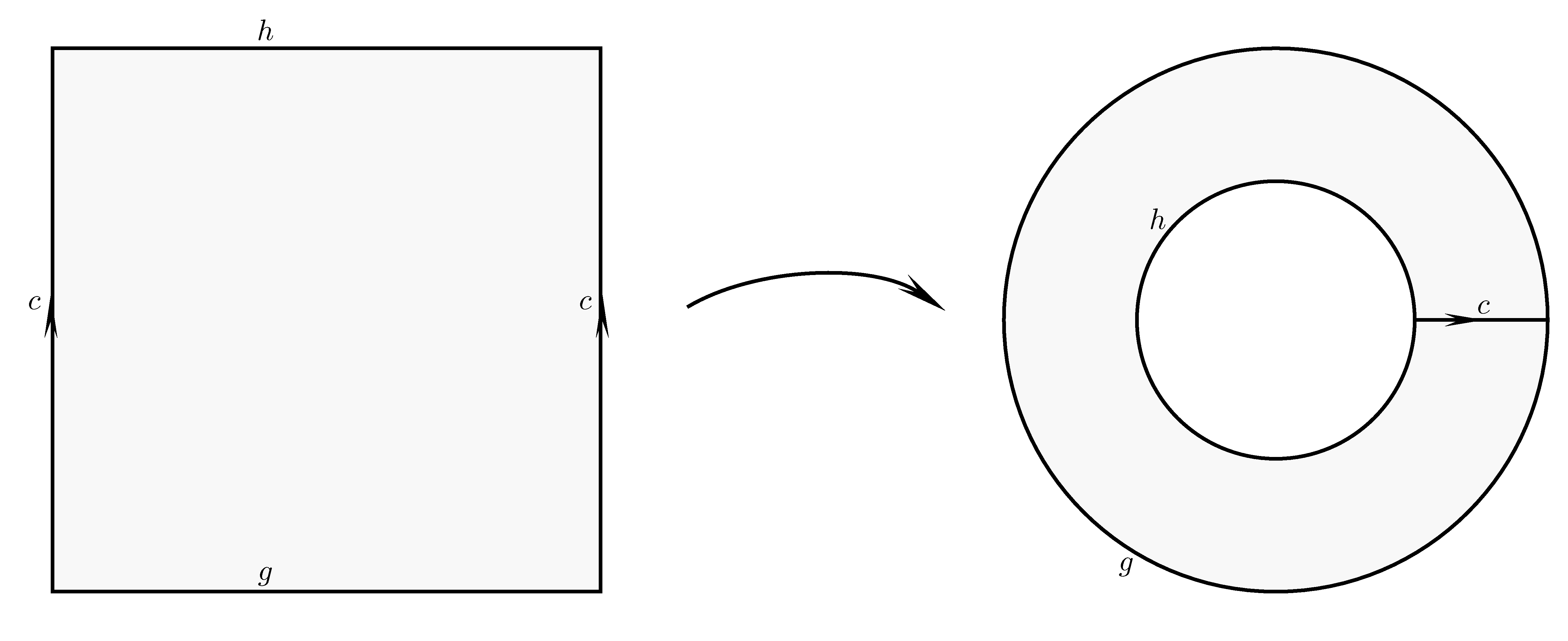
Figure 2: A square can be mapped into an annulus, by identifying a pair of opposite sides.

Proof of Lemma 3.4.

By an average argument, we find $z_{0}\in[-L/4,\,L/4]$ such that

(3.8) $$\left\|\nabla_{\top}g\right\|^{2}_{L^{2}(\partial B^{2}_{r}\times\{z_{0}\})}\leq\frac{8}{L}\left\|\nabla_{\top}g\right\|^{2}_{L^{2}(\Gamma)}.$$

To avoid notation, we assume WLOG that $z_{0}=0$. We construct an $\mathscr{N}$-valued map $\tilde{P}$, defined over the “cylindrical annulus” $(B^{2}_{r}\setminus B^{2}_{r/2})\times[-L,\,L]$, such that

$$\tilde{P}\left(\rho e^{i\theta},\,z\right)=\begin{cases}g(re^{i\theta},\,z)\qquad\textrm{for }\rho=r\\ g(re^{i\theta},\,0)\qquad\textrm{for }\rho=r/2,\end{cases}$$

where $(\rho,\,\theta,\,z)\in[0,\,r]\times[0,\,2\pi]\times[-L,\,L]$ are the cylindrical coordinates. Then, since $\tilde{P}$ restricted to $\partial B^{2}_{r/2}\times[-L,\,L]$ is independent of the $z$-variable, we can apply Lemma 3.3 to construct an extension in the inner cylinder $B^{2}_{r/2}\times[-L,\,L]$.

The map $\tilde{P}$ is defined as follows:

$$\tilde{P}(\rho e^{i\theta},\,z):=\begin{cases}g\left(re^{i\theta},\,z^{\prime}(\rho,\,z)\right)&\textrm{if }\rho_{0}(\rho,\,z)\leq\rho\leq r\textrm{ and }|z|\leq L\\ g(re^{i\theta},\,0)&\textrm{if }r/2\leq\rho<\rho_{0}(\rho,\,z)\textrm{ and }|z|\leq L,\end{cases}$$

where

$$z^{\prime}(\rho,\,z):=\dfrac{2L}{r}\operatorname{sign}(z)(\rho-r)+z,\qquad\rho_{0}(\rho,\,z):=r-\dfrac{r}{2L}|z|.$$

Note that $|z^{\prime}(\rho,\,z)|\leq L$ if $\rho_{0}(\rho,\,z)\leq\rho\leq r$ and $|z|\leq L$. We compute the $H^{1}$-seminorm of $\tilde{P}$. For simplicity, we restrict our attention to the upper half-cylinder. We have

$$\begin{split}&\|\nabla\tilde{P}\|^{2}_{L^{2}((B^{2}_{r}\setminus B^{2}_{r/2})\times[0,\,L])}\\ &\qquad=\int_{0}^{2\pi}\int_{0}^{L}\int_{\rho_{0}(\rho,\,z)}^{r}\left\{\left(\frac{4L^{2}}{r^{2}}+1\right)\rho\left|\partial_{z}g\right|^{2}\left(re^{i\theta},\,z^{\prime}(\rho,\,z)\right)+\rho^{-1}\left|\partial_{\theta}g\right|^{2}\left(re^{i\theta},\,z^{\prime}(\rho,\,z)\right)\right\}\,\mathrm{d}\rho\,\mathrm{d}z\,\mathrm{d}\theta\\ &\qquad\qquad\qquad+\int_{0}^{2\pi}\int_{0}^{L}\int_{r/2}^{\rho_{0}(\rho,\,z)}\rho^{-1}\left|\partial_{\theta}g\right|^{2}\left(re^{i\theta},\,0\right)\,\mathrm{d}\rho\,\mathrm{d}z\,\mathrm{d}\theta\\ &\qquad\leq\frac{r}{2L}\int_{0}^{2\pi}\int_{0}^{L}\int_{0}^{z}\left\{\left(\frac{4L^{2}}{r^{2}}+1\right)r\left|\partial_{z}g\right|^{2}+2r^{-1}\left|\partial_{\theta}g\right|^{2}\right\}(re^{i\theta},\,\xi)\,\mathrm{d}\xi\,\mathrm{d}z\,\mathrm{d}\theta\\ &\qquad\qquad\qquad+(\log 2)L\int_{0}^{2\pi}\left|\partial_{\theta}g\right|^{2}\left(re^{i\theta},\,0\right)\,\mathrm{d}\theta\\ &\qquad\leq r\left(\frac{4L^{2}}{r^{2}}+1\right)\int_{0}^{2\pi}\int_{0}^{L}\left\{r\left|\partial_{z}g\right|^{2}+r^{-1}\left|\partial_{\theta}g\right|^{2}\right\}(re^{i\theta},\,\xi)\,\mathrm{d}\xi\,\mathrm{d}\theta+(\log 2)L\int_{0}^{2\pi}\left|\partial_{\theta}g\right|^{2}\left(re^{i\theta},\,0\right)\,\mathrm{d}\theta.\end{split}$$

An analogous estimates holds on the lower half-cylinder. Therefore,

$$\|\nabla\tilde{P}\|^{2}_{L^{2}((B^{2}_{r}\setminus B^{2}_{r/2})\times[-L,\,L])}\leq\left(\frac{4L^{2}}{r}+r\right)\left\|\nabla_{\top}g\right\|^{2}_{L^{2}(\Gamma)}+(\log 2)rL\left\|\nabla_{\top}g\right\|^{2}_{L^{2}(\partial B^{2}_{r}\times\{0\})}$$

and so, due to (3.8), we have

(3.9) $$\|\nabla\tilde{P}\|^{2}_{L^{2}((B^{2}_{r}\setminus B^{2}_{r/2})\times[-L,\,L])}\leq C\left(\frac{L^{2}}{r}+r\right)\left\|\nabla_{\top}g\right\|^{2}_{L^{2}(\Gamma)}.$$

By applying Lemma 3.3 (and (3.8)) to $g(\cdot,\,0)$, we find an extension $\tilde{P}_{\varepsilon}\in H^{1}(B^{2}_{r/2},\,\mathbf{S}_{0})$ which satisfies

(3.10) $$E_{\varepsilon}(\tilde{P}_{\varepsilon},\,B^{2}_{r/2})\leq\kappa_{*}\log\frac{r}{\varepsilon}+\frac{Cr}{L}\left\|\nabla_{\top}g\right\|^{2}_{L^{2}(\Gamma)}+C.$$

Define the map $P$ by letting $P(\rho e^{i\theta},\,z):=\tilde{P}(\rho e^{i\theta},\,z)$ if $r/2<\rho\leq r$ and $P_{\varepsilon}(\rho e^{i\theta},\,z):=\tilde{P}_{\varepsilon}(\rho e^{i\theta})$ if $\rho\leq r/2$. By integrating (3.9) with respect to $z\in[-L,\,L]$, and combining the resulting inequality with (3.9), we give an upper bound for the energy of $P_{\varepsilon}$ on $\Lambda$. Moreover, there holds

$$\begin{split}&\|\nabla\tilde{P}\|^{2}_{L^{2}((B^{2}_{r}\setminus B^{2}_{r/2})\times\{L\})}\\ &\qquad=\int_{0}^{2\pi}\int_{r/2}^{r}\left\{\left(\frac{4L^{2}}{r^{2}}+1\right)\rho\left|\partial_{z}g\right|^{2}\left(re^{i\theta},\,z^{\prime}(\rho,\,L)\right)+\rho^{-1}\left|\partial_{\theta}g\right|^{2}\left(re^{i\theta},\,z^{\prime}(\rho,\,L)\right)\right\}\,\mathrm{d}\rho\,\mathrm{d}\theta\\ &\qquad\leq\frac{r}{2L}\int_{0}^{2\pi}\int_{0}^{L}\left\{\left(\frac{4L^{2}}{r^{2}}+1\right)r\left|\partial_{z}g\right|^{2}+2r^{-1}\left|\partial_{\theta}g\right|^{2}\right\}(re^{i\theta},\,\xi)\,\mathrm{d}\xi\,\mathrm{d}\theta\\ &\qquad\leq\frac{r}{L}\left(\frac{4L^{2}}{r^{2}}+1\right)\left\|\nabla_{\top}g\right\|^{2}_{L^{2}(\Gamma)}.\end{split}$$

This inequality combined with (3.10), gives an upper bound for the energy of $P_{\varepsilon}$ on $B^{2}_{r}\times\{L\}$; a similar inequality holds on $B^{2}_{r}\times\{-L\}$. This concludes the proof. ∎

3.2 Luckhaus’ lemma and its variants

When dealing with the asymptotic analysis for minimizers $Q_{\varepsilon}$ of (LG_ε), we will be confronted with the following issue. Suppose that $r>0$ and $B_{r}\subseteq\Omega$. Given a map $P_{\varepsilon}\colon B_{r}\to\mathbf{S}_{0}$, we wish to compare the energy of $P_{\varepsilon}$ with the energy of a minimizer $Q_{\varepsilon}$. However, it may happen that $P_{\varepsilon}\neq Q_{\varepsilon}$ on $\partial B_{r}$, so $P_{\varepsilon}$ is not an admissible comparison map. To correct this, we need to construct a function which interpolates between $P_{\varepsilon}$ and $Q_{\varepsilon}$ over a thin spherical shell.

In general terms, the problem may be stated as follows. Fix a parameter $0<\epsilon<1$ (in the application, $\epsilon$ will depend on both $\varepsilon$ and $r$). Let $u_{\epsilon}$, $v_{\epsilon}\colon\partial B_{1}\to\mathbf{S}_{0}$ be two given maps in $H^{1}$. We look for a spherical shell $A_{\epsilon}:=B_{1}\setminus B_{1-h(\epsilon)}$ of (small) thickness $h(\epsilon)>0$ and a map $\varphi_{\epsilon}\colon A_{\epsilon}\to\mathbf{S}_{0}$, such that

(3.11) $$\varphi_{\epsilon}(x)=u_{\epsilon}(x)\quad\textrm{and}\quad\varphi_{\epsilon}(x-h(\epsilon)x)=v_{\epsilon}(x)\qquad\textrm{for }\mathscr{H}^{2}\textrm{-a.e. }x\in\partial B_{1}$$

and the energy $E_{\varepsilon}(\varphi_{\epsilon},\,A_{\epsilon})$ satisfies a suitable bound. Moreover, in some circumstances only the function $u_{\epsilon}$ is prescribed, and we need to find both a map $v_{\epsilon}\colon\partial B_{1}\to\mathscr{N}$ and the interpolating function $\varphi_{\epsilon}$.

Luckhaus proved an interesting interpolation lemma (see [49, Lemma 1]), which turned out to be useful in several applications. When the two maps $u_{\epsilon}$, $v_{\epsilon}$ take values in the manifold $\mathscr{N}$, Luckhaus’ lemma gives an extension $\varphi_{\epsilon}$ satisfying (3.11) and

$$\sup_{x\in A_{\epsilon}}\operatorname{dist}(\varphi_{\epsilon}(x),\,\mathscr{N})+\int_{A_{\epsilon}}\left|\nabla\varphi_{\epsilon}\right|^{2}\leq C(u_{\epsilon},\,v_{\epsilon},\,h(\epsilon)).$$

For the convenience of the reader, and for future reference, we recall Luckhaus’ lemma. Since the potential $\epsilon^{-2}f$ is not taken into account here, we drop the subscript $\epsilon$ in the notation.

Lemma 3.7 (Luckhaus, [49]).

For any $\beta\in(1/2,\,1)$, there exists a constant $C>0$ with this property. For any fixed numbers $0<\lambda\leq 1/2$, $0<\sigma<1$ and any $u,\,v\in H^{1}(\partial B_{1},\,\mathscr{N})$, set

$$K:=\int_{\partial B_{1}}\left\{\left|\nabla u\right|^{2}+\left|\nabla v\right|^{2}+\frac{\left|u-v\right|^{2}}{\sigma^{2}}\right\}\,\mathrm{d}\mathscr{H}^{2}.$$

Then, there exists a function $\varphi\in H^{1}(B_{1}\setminus B_{1-\lambda},\,\mathbf{S}_{0})$ satisfying (3.11),

$$\operatorname{dist}(\varphi(x),\,\mathscr{N})\leq C\sigma^{1-\beta}\lambda^{-1/2}K^{1/2}$$

for a.e. $x\in B_{1}\setminus B_{1-\lambda}$ and

$$\int_{B_{1}\setminus B_{1-\lambda}}\left|\nabla\varphi\right|^{2}\leq C\lambda\left(1+\sigma^{2}\lambda^{-2}\right)K.$$

The idea of the proof is illustrated in Figure 3. One constructs a grid on the sphere $\partial B_{1}$ with suitable properties. The map $\varphi$ is defined by linear interpolation between $u$ and $v$ on the boundary of the cells. Inside each cell, $\varphi$ is defined by a homogeneous extension. By choosing carefully the grid on $\partial B_{1}$, and using Sobolev embeddings, one can bound the $L^{\infty}$-distance between $u$ and $v$ on the boundary of the cells, in terms of $K$. This yields bounds both on $\operatorname{dist}(\varphi(x),\,\mathscr{N})$ and on the gradient of $\varphi$.

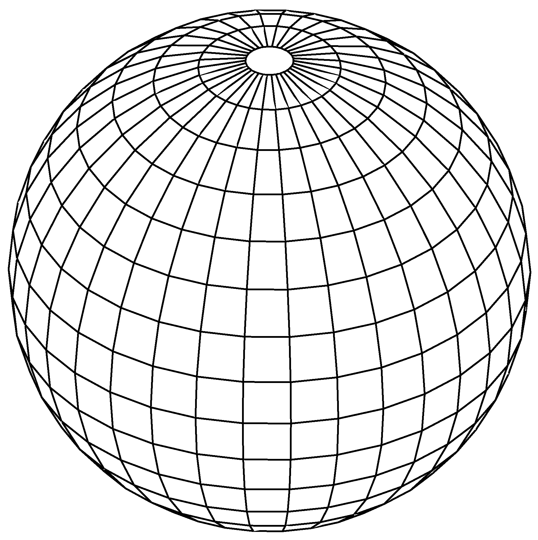
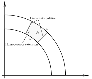
Figure 3: Left: a grid on a sphere. Right: the Luckhaus’ construction. Given two maps $u_{\epsilon}$, $v_{\epsilon}$ (respectively defined on the outer and inner boundary of a thin spherical shell), we construct a map $\varphi_{\epsilon}$ by using linear interpolation on the boundary of the cells, and homogeneous extension inside each cell.

We will discuss here a couple of variants of this lemma. In our first result, we suppose that only the map $u_{\epsilon}\colon\partial B_{1}\to\mathbf{S}_{0}$ is prescribed, so we need to find both $v_{\epsilon}\colon\partial B_{1}\to\mathscr{N}$ and $\varphi_{\epsilon}$. Approximating $u_{\epsilon}$ with a $\mathscr{N}$-valued map $v_{\epsilon}$ may be impossible, due to topological obstructions. However, this is possible if the energy of $u_{\epsilon}$ is small, compared to $|\log\epsilon|$. More precisely, we assume that

(3.12) $$E_{\epsilon}(u_{\epsilon},\,\partial B_{1})\leq\eta_{0}\left|\log\epsilon\right|$$

for some small constant $\eta_{0}>0$. For technical reasons, we also require a $L^{\infty}$-bound on $u_{\epsilon}$, namely

(3.13) $$\left\|u_{\epsilon}\right\|_{L^{\infty}(\partial B_{1})}\leq\kappa$$

where $\kappa$ is an $\epsilon$-independent constant. In the applications, $u_{\epsilon}$ will be a Landau-de Gennes minimizer and (3.13) will be satisfied, because of (H).

Proposition 3.8.

For any $\kappa>0$, there exist positive numbers $\eta_{0}$, $\epsilon_{1}$, $C$ with the following property. For any $0<\eta\leq\eta_{0}$, any $0<\epsilon\leq\epsilon_{1}$ and any $u_{\epsilon}\in(H^{1}\cap L^{\infty})(\partial B_{1},\,\mathbf{S}_{0})$ satisfying (3.12)–(3.13), there exist maps $v_{\epsilon}\in H^{1}(\partial B_{1},\,\mathscr{N})$ and $\varphi_{\epsilon}\in H^{1}(B_{1}\setminus B_{1-h(\epsilon)},\,\mathbf{S}_{0})$ which satisfy (3.11),

(3.14) $$\frac{1}{2}\int_{\partial B_{1}}\left|\nabla v_{\epsilon}\right|^{2}\,\mathrm{d}\mathscr{H}^{2}\leq CE_{\epsilon}(u_{\epsilon},\,\partial B_{1}),$$

(3.15) $$E_{\epsilon}(\varphi_{\epsilon},\,B_{1}\setminus B_{1-h(\epsilon)})\leq Ch(\epsilon)E_{\epsilon}(u_{\epsilon},\,\partial B_{1})$$

for $h(\epsilon):=\epsilon^{1/2}|\log\epsilon|$.

We will discuss the proof of this proposition later on. Before that, we remark that $v_{\epsilon}$ effectively approximates $u_{\epsilon}$, i.e. their distance — measured in a suitable norm — tends to $0$ as $\epsilon\to 0$.

Corollary 3.9.

Under the same assumptions of Proposition 3.8, there holds

$$\left\|u_{\epsilon}-v_{\epsilon}\right\|_{L^{2}(\partial B_{1})}\leq Ch^{1/2}(\epsilon)E^{1/2}_{\epsilon}(u_{\epsilon},\,\partial B_{1}).$$

Notice that the right-had side tends to $0$ as $\epsilon\to 0$, due to (3.12) and the choice of $h(\epsilon)$.

Proof.

We can estimate the $L^{2}$-distance between $u_{n}$ and $v_{n}$ thanks to (3.11):

$$\begin{split}\left\|u_{\epsilon}-v_{\epsilon}\right\|_{L^{2}(\partial B_{1})}^{2}&\stackrel{{\scriptstyle\eqref{phi bd value}}}{{=}}\int_{\partial B_{1}}\left|\varphi_{\epsilon}(x)-\varphi_{\epsilon}(x-h(\epsilon)x)\right|^{2}\,\mathrm{d}\mathscr{H}^{2}(x)\\ &=\int_{\partial B_{1}}\left|\int_{1-h(\epsilon)}^{1}\nabla\varphi_{\epsilon}(tx)x\,\mathrm{d}t\,\right|^{2}\,\mathrm{d}\mathscr{H}^{2}(x).\end{split}$$

Then, by Hölder inequality,

$$\begin{split}\left\|u_{\epsilon}-v_{\epsilon}\right\|_{L^{2}(\partial B_{1})}^{2}&\leq h(\epsilon)\int_{\partial B_{1}}\int_{1-h(\epsilon)}^{1}\left|\nabla\varphi_{\epsilon}(tx)\right|^{2}\,\mathrm{d}t\,\mathrm{d}\mathscr{H}^{2}(x)\\ &\leq\frac{h(\epsilon)}{(1-h(\epsilon))^{2}}E_{\epsilon}(\varphi_{\epsilon},\,B_{1}\setminus B_{1-h(\epsilon)})\stackrel{{\scriptstyle\eqref{phi energy}}}{{\leq}}Ch(\epsilon)E_{\epsilon}(u_{\epsilon},\,\partial B_{1}).\qed\end{split}$$

Combining Lemma 3.7 and Proposition 3.8, we obtain a third extension result. In this case, both the boundary values $u$, $v$ are prescribed and, unlike Luckhaus’ lemma, we provide a control over the potential energy of the extension $\epsilon^{-2}f(\varphi_{\epsilon})$.

Proposition 3.10.

Let $\{\sigma_{\epsilon}\}_{\epsilon>0}$ be a positive sequence such that $\sigma_{\epsilon}\to 0$, and let $u_{\epsilon}$, $v_{\epsilon}$ be given functions in $H^{1}(\partial B_{1},\,\mathbf{S}_{0})$. For all $\epsilon>0$, assume that $u_{\epsilon}$ satisfies (3.13), that $v_{\epsilon}(x)\in\mathscr{N}$ for $\mathscr{H}^{2}$-a.e. $x\in\partial B_{1}$ and that

(3.16) $$\int_{\partial B_{1}}\left\{\left|\nabla u_{\epsilon}\right|^{2}+\frac{1}{\epsilon^{2}}f(u_{\epsilon})+\left|\nabla v_{\epsilon}\right|^{2}+\frac{\left|u_{\epsilon}-v_{\epsilon}\right|^{2}}{\sigma_{\epsilon}^{2}}\right\}\,\mathrm{d}\mathscr{H}^{2}\leq C$$

for an $\epsilon$-independent constant $C$. Set

$$\nu_{\epsilon}:=h(\epsilon)+\left(h^{1/2}(\epsilon)+\sigma_{\epsilon}\right)^{1/4}\left(1-h(\epsilon)\right).$$

Then, there exist a number $\epsilon_{1}>0$ and, for $0<\epsilon\leq\epsilon_{1}$, a function $\varphi_{\epsilon}\in H^{1}(B_{1}\setminus B_{1-\nu_{\epsilon}},\,\mathbf{S}_{0})$ which satisfies (3.11) and

$$E(\varphi_{\epsilon},\,B_{1}\setminus B_{1-\nu_{\epsilon}})\leq C\nu_{\epsilon}.$$

The assumption (3.16) could be relaxed by requiring just a logarithmic bound, of the order of $\eta_{0}|\log\epsilon|$ for small $\eta_{0}>0$, with additional assumptions on $\sigma_{\epsilon}$. However, the result as it is presented here suffices for our purposes.

Proof of Proposition 3.10.

Thanks to (3.16) and (3.13), we can apply Proposition 3.8 to the function $u_{\epsilon}$. We obtain two maps $w_{\epsilon}\in H^{1}(\partial B_{1},\,\mathscr{N})$ and $\varphi_{\epsilon}^{1}\in H^{1}(B_{1}\setminus B_{1-h(\epsilon)},\,\mathbf{S}_{0})$, which satisfy

$$\varphi_{\epsilon}^{1}(x)=u_{\epsilon}(x)\quad\textrm{and}\quad\varphi_{\epsilon}^{1}(x-h(\epsilon)x)=w_{\epsilon}(x)\qquad\textrm{for }\mathscr{H}^{2}\textrm{-a.e. }x\in\partial B_{1},$$

$$\int_{\partial B_{1}}\left|\nabla w_{\epsilon}\right|^{2}\,\mathrm{d}\mathscr{H}^{2}\leq C,$$

(3.17) $$E_{\epsilon}(\varphi_{\epsilon}^{1},\,B_{1}\setminus B_{1-h(\epsilon)})\leq Ch(\epsilon).$$

Corollary 3.9, combined with (3.16), entails

$$\left\|w_{\epsilon}-v_{\epsilon}\right\|_{L^{2}(\partial B_{1})}\leq\left\|w_{\epsilon}-u_{\epsilon}\right\|_{L^{2}(\partial B_{1})}+\left\|u_{\epsilon}-v_{\epsilon}\right\|_{L^{2}(\partial B_{1})}\leq C\left(h^{1/2}(\epsilon)+\sigma_{\epsilon}\right).$$

Therefore, setting $\tilde{\sigma}_{\epsilon}:=h^{1/2}(\epsilon)+\sigma_{\epsilon}$, we have

$$\int_{\partial B_{1}}\left\{\left|\nabla w_{\epsilon}\right|^{2}+\left|\nabla v_{\epsilon}\right|^{2}+\frac{\left|w_{\epsilon}-v_{\epsilon}\right|^{2}}{\tilde{\sigma}_{\epsilon}^{2}}\right\}\,\mathrm{d}\mathscr{H}^{2}\leq C$$

Then, we can apply Lemma 3.7 to $v_{\epsilon}$ and $w_{\epsilon}$, choosing $\sigma=\tilde{\sigma}_{\epsilon}$, $\beta=3/4$ and $\lambda:=\tilde{\sigma}_{\epsilon}^{1/4}$. By rescaling, we find a map $\varphi_{\epsilon}^{2}\in H^{1}(B_{1-h(\epsilon)}\setminus B_{\nu_{\epsilon}},\,\mathbf{S}_{0})$ which satisfies

$$\int_{B_{1-h(\epsilon)}\setminus B_{\nu_{\epsilon}}}\left|\nabla\varphi_{\epsilon}^{2}\right|^{2}\leq C\tilde{\sigma}_{\epsilon}^{1/4}\left(1-h(\epsilon)\right)$$

(3.18) $$\operatorname{dist}(\varphi_{\epsilon}^{2}(x),\,\mathscr{N})\leq C\tilde{\sigma}_{\epsilon}^{1/8}\qquad\textrm{for all }x\in B_{1-h(\epsilon)}\setminus B_{\nu_{\epsilon}}.$$

Since $\tilde{\sigma}_{\epsilon}\to 0$, there exists $\epsilon_{1}>0$ such that $\varphi_{\epsilon}^{2}(x)\notin\mathscr{C}$ for any $0<\epsilon\leq\epsilon_{1}$ and $x$. Therefore, the function

$$\varphi_{\epsilon}(x):=\begin{cases}\varphi_{\epsilon}^{1}(x)&\textrm{if }x\in B_{1}\setminus B_{1-h(\epsilon)}\\ \varrho\circ\varphi_{\epsilon}^{2}(x)&\textrm{if }x\in B_{1-h(\epsilon)}\setminus B_{\nu_{\epsilon}}\end{cases}$$

is well-defined, belongs to $H^{1}(B_{1}\setminus B_{\nu_{\epsilon}},\,\mathscr{N})$, satisfies (3.11) and

$$E_{\epsilon}(\varphi_{\epsilon},\,B_{1}\setminus B_{\nu_{\epsilon}})=E_{\epsilon}(\varphi_{\epsilon}^{1},\,B_{1}\setminus B_{1-h(\epsilon)})+\int_{B_{1-h(\epsilon)}\setminus B_{\nu_{\epsilon}}}\left|\nabla\varphi_{\epsilon}^{2}\right|^{2}\stackrel{{\scriptstyle\eqref{interp3,1}\textrm{--}\eqref{interp3,2}}}{{\leq}}C\nu_{\epsilon}.\qed$$

Subsections 3.3–3.5 are devoted to the proof of Proposition 3.8, which we sketch here. From now on, we assume that there exists a positive constant $M$ such that

(M_ϵ) $$E_{\epsilon}(u_{\epsilon},\,\partial B_{1})\leq M\left|\log\epsilon\right|\qquad\textrm{for all }0<\epsilon<1.$$

The assumption (3.12) clearly implies (M_ϵ). As in Luckhaus’ arguments, the key ingredient of the construction is the choice of a grid on the unit sphere $\partial B_{1}$, with special properties. In Subsection 3.3 we construct a family of grids $\{\mathscr{G}^{\epsilon}\}$, whose cells have size controlled by $h(\epsilon)$, and we prove that there exists $\epsilon_{1}>0$ such that

$$\operatorname{dist}(u_{\epsilon}(x),\,\mathscr{N})\leq\delta_{0}\qquad\textrm{for any }\epsilon\in(0,\,\epsilon_{1})\textrm{ and any }x\in R^{\epsilon}_{1}.$$

Here $R^{\epsilon}_{1}$ denotes the $1$-skeleton of $\mathscr{G}^{\epsilon}$, i.e. the union of the boundaries of all the cells, and $\delta_{0}$ is given by Lemma 2.4. In particular, the composition $\varrho\circ u_{\epsilon}$ is well-defined on $R^{\epsilon}_{1}$ when $\epsilon<\epsilon_{1}$. We wish to extend $\varrho\circ u_{\epsilon}$ to a map $v_{\epsilon}\colon\partial B_{1}\to\mathscr{N}$. This may be impossible, depending on the homotopy properties of $u_{\epsilon}$. A sufficient condition for the existence of $v_{\epsilon}$ is the following:

1. For any $2$-cell $K$ of $\mathscr{G}^{\epsilon}$, the loop ${\varrho\circ u_{\epsilon}}_{|\partial K}\colon\partial K\to\mathscr{N}$ is homotopically trivial.

This condition makes sense for any $u_{\epsilon}\in H^{1}(\partial B_{1},\,\mathbf{S}_{0})$, for we construct $\mathscr{G}^{\epsilon}$ in such a way that $u_{\epsilon}$ restricted to $R^{\epsilon}_{1}$ belongs to $H^{1}\hookrightarrow C^{0}$.

In Subsection 3.4, we assume that (M_ϵ) and (C_$\epsilon$) hold and we construct a function $v_{\epsilon}\in H^{1}(\partial B_{1},\,\mathscr{N})$, whose energy is controlled by the energy of $u_{\epsilon}$. Basically, we extend ${\varrho\circ u_{\epsilon}}_{|\partial K}$ inside every $2$-cell $K\in\mathscr{G}^{\epsilon}$, which is possible by Condition (C_$\epsilon$). Once $v_{\epsilon}$ is known, we construct $\varphi_{\epsilon}$ by Luckhaus’ method. Particular care must be taken here, as we need to bound the potential energy of $\varphi_{\epsilon}$ as well.

Finally, in Subsection 3.5 we show that the logarithmic bound (3.12), for a small enough constant $\eta_{0}$, implies that Condition (C_$\epsilon$) is satisfied. Arguing by contra-position, we assume that (C_$\epsilon$) is not satisfied. Then, ${\varrho\circ u_{\epsilon}}_{|\partial K}$ is non-trivial for at least one $2$-cell $K\in\mathscr{G}^{\epsilon}$. In this case, using Jerrard-Sandier type lower bounds, we prove that the energy $E_{\epsilon}(u_{\epsilon},\,\partial B_{1})$ blows up at least as $\eta_{1}|\log\epsilon|$ for some $\eta_{1}>0$. Taking $\eta_{0}<\eta_{1}$, we have a contradiction because of (3.12), so the proof is complete.

3.3 Good grids on the sphere

Consider a decomposition of $\partial B_{1}$ of the form

$$\partial B_{1}=\bigcup_{j=0}^{2}\bigcup_{i=1}^{k_{j}}K_{i,j},$$

where the sets $K_{i,j}$ are mutually disjoint, and each $K_{i,j}$ is bilipschitz equivalent to a $j$-dimensional ball. The collection of all the $K_{i,j}$’s will be called a grid on $\partial B_{1}$. Each $K_{i,j}$ will be called a $j$-cell of the grid. We define the $j$-skeleton of the grid as

$$R_{j}:=\bigcup_{i=1}^{k_{j}}K_{i,j}\qquad\textrm{for }j\in\{0,\,1,\,2\}.$$

For our purposes, we need to consider grids with some special properties.

Definition 3.1.

Let $h\colon(0,\,\epsilon_{1}]\to(0,\,+\infty)$ be a fixed function. A family of grids $\mathscr{G}:=\{\mathscr{G}^{\epsilon}\}_{0<\epsilon\leq\epsilon_{1}}$ will be called a good family of grids of size $h$ if there exists a constant $C_{\mathscr{G}}>0$ which satisfies the following properties.

1. For each $\epsilon$, $i$, $j$, there exists a bilipschitz homeomorphism $\varphi^{\epsilon}_{i,j}\colon K^{\epsilon}_{i,j}\to B^{j}_{h(\epsilon)}$ such that

   $$\left\|\mathrm{D}\varphi^{\epsilon}_{i,j}\right\|_{L^{\infty}}+\left\|\mathrm{D}(\varphi^{\epsilon}_{i,j})^{-1}\right\|_{L^{\infty}}\leq C_{\mathscr{G}}.$$

2. For all $p\in\{1,\,2,\,\ldots,k_{1}\}$ we have

   $$\#\left\{q\in\{1,\,2,\,\ldots,k_{2}\}\colon K^{\epsilon}_{p,1}\subseteq K^{\epsilon}_{q,2}\right\}\leq C_{\mathscr{G}},$$

   i.e., each $1$-cell is contained in the boundary of at most $C_{\mathscr{G}}$ $2$-cells.

3. We have

   $$E_{\epsilon}(u_{\epsilon},\,R^{\epsilon}_{1})\leq C_{\mathscr{G}}h^{-1}(\epsilon)\,E_{\epsilon}(u_{\epsilon},\,\partial B_{1}),$$

   where $R^{\epsilon}_{1}$ denotes the $1$-skeleton of $\mathscr{G}^{\epsilon}$.

4. There holds

   $$\int_{R^{\epsilon}_{1}}f(u_{\epsilon})\,\mathrm{d}\mathscr{H}^{1}\leq C_{\mathscr{G}}h^{-1}(\epsilon)\int_{\partial B_{1}}f(u_{\epsilon})\,\mathrm{d}\mathscr{H}^{2}.$$

Of course, this definition depends on the family $\{u_{\epsilon}\}$, which we assume to be fixed once and for all.

Lemma 3.11.

For any strictly positive function $h$, a good family of grids of size $h$ exists.

Proof.

On the unit cube $\partial[0,\,1]^{3}$, consider the uniform grid of size $\lceil h^{-1}(\epsilon)\rceil^{-1}$, i.e. the grid spanned by the points

$$\left(\lceil h^{-1}(\epsilon)\rceil^{-1}\mathbb{Z}^{3}\right)\cap\partial[0,\,1]^{3}$$

(where $\lceil x\rceil$ is, by the definition, the smallest integer $k$ such that $k\geq x$). By applying a bilipschitz homeomorphism $[0,\,1]^{3}\to\overline{B}_{1}$, one obtains a grid $\mathscr{F}^{\epsilon}$ on $\partial B_{1}$ which satisfy (G₁)–(G₂). Denote by $T^{\epsilon}_{1}$ the $1$-skeleton of $\mathscr{F}^{\epsilon}$. By an average argument, as in [49, Lemma 1], we find a rotation $\omega\in\mathrm{SO}(3)$ such that

$$E_{\epsilon}(u_{\epsilon},\,\omega(T^{\epsilon}_{1}))\leq Ch^{-1}(\epsilon)\,E_{\epsilon}(u_{\epsilon},\,\partial B_{1})$$

and

$$\int_{\omega(T^{\epsilon}_{1})}f(u_{\epsilon})\,\mathrm{d}\mathscr{H}^{1}\leq Ch^{-1}(\epsilon)\int_{\partial B_{1}}f(u_{\epsilon})\,\mathrm{d}\mathscr{H}^{2}.$$

Thus,

$$\mathscr{G}^{\epsilon}:=\left\{\omega(K)\colon K\in\mathscr{F}^{\epsilon}\right\}$$

is a good family of grids of size $h$. ∎

Good families of grids enjoy the following property.

Lemma 3.12.

Let $\mathscr{G}$ be a good family of grids on $\partial B_{1}$, of size $h$. Assume that (M_ϵ) holds, and that there exists $\alpha\in(0,\,1)$ such that

(3.19) $$\lim_{\epsilon\to 0}\epsilon^{\alpha}h^{-1}(\epsilon)=0.$$

Then, there holds

$$\lim_{\epsilon\to 0}\sup_{x\in R^{\epsilon}_{1}}\operatorname{dist}(u_{\epsilon}(x),\,\mathscr{N})=0.$$

Proof.

The arguments below are adapted from [1, Lemmas 3.4 and 3.10] (the reader is also referred to [14, Lemmas 2.2, 2.3 and 2.4]). Since the Landau-de Gennes potential satisfies (F₂) by Lemma 2.4, there exist positive numbers $\beta$, $C$ and a continuous function $\psi\colon[0,\,+\infty)\to\mathbb{R}$ such that

$$\begin{cases}\psi(s)=\beta s^{2}&\textrm{for }0\leq s<\delta_{0}\\ 0<\psi(s)\leq C&\textrm{for }s\geq\delta_{0}\\ \psi(\operatorname{dist}(v,\,\mathscr{N}))\leq f(v)&\textrm{for any }v\in\mathbf{S}_{0}.\end{cases}$$

Denote by $G$ a primitive of $\psi^{1/6}$, and set $d_{\epsilon}:=\operatorname{dist}(u_{\epsilon},\,\mathscr{N})$. Since the function $\operatorname{dist}(\cdot,\,\mathscr{N})$ is $1$-Lipschitz continuous, we have $d_{\epsilon}\in H^{1}(\Omega,\,\mathbb{R})$ and $\left|\nabla d_{\epsilon}\right|\leq\left|\nabla u_{\epsilon}\right|$. Moreover, $\psi(d_{\epsilon})\leq f(u_{\epsilon})$ by construction of $\psi$. Thus, (M_ϵ) and (G₃) entail

$$h(\epsilon)\int_{R^{\epsilon}_{1}}\left\{\frac{1}{2}\left|\nabla d_{\epsilon}\right|^{2}+\epsilon^{-2}\psi(d_{\epsilon})\right\}\,\mathrm{d}\mathscr{H}^{1}\leq MC_{\mathscr{G}}|\log\epsilon|.$$

By applying Young’s inequality $a+b\geq Ca^{3/4}b^{1/4}$, we obtain

(3.20) $$\begin{split}MC_{\mathscr{G}}|\log\epsilon|&\geq C\epsilon^{-1/2}h(\epsilon)\int_{R^{\epsilon}_{1}}\left|\nabla d_{\epsilon}\right|^{3/2}\psi^{1/4}(d_{\epsilon})\,\mathrm{d}\mathscr{H}^{1}\\ &=C\epsilon^{-1/2}h(\epsilon)\int_{R^{\epsilon}_{1}}\left|\nabla G(d_{\epsilon})\right|^{3/2}\,\mathrm{d}\mathscr{H}^{1}.\end{split}$$

Fix a $1$-cell $K$ of $\mathscr{G}^{\epsilon}$. We control the oscillations of $G(d_{\epsilon})$ over $K$ thanks to the Sobolev embedding $W^{1,3/2}(K)\hookrightarrow C^{0}(K)$ and (3.20):

$$\begin{split}\left(\underset{K}{\mathrm{osc}\,}G(d_{\epsilon})\right)^{3/2}&\leq Ch^{1/2}(\epsilon)\int_{K}\left|\nabla G(d_{\epsilon})\right|^{3/2}\,\mathrm{d}\mathscr{H}^{1}\\ &=C\epsilon^{1/2}h^{-1/2}(\epsilon)\left|\log\epsilon\right|.\end{split}$$

In view of (3.19), we obtain

$$\underset{R^{\epsilon}_{1}}{\mathrm{osc}\,}G(d_{\epsilon})\to 0$$

as $\epsilon\to 0$. The function $G$ is a continuous and strictly increasing, so $G$ has a continuous inverse. This implies

(3.21) $$\underset{R^{\epsilon}_{1}}{\mathrm{osc}\,}d_{\epsilon}\to 0$$

as $\epsilon\to 0$. On the other hand, (M_ϵ), (G₃) and (3.19) yield

(3.22) $$\fint_{K}\psi(d_{\epsilon})\,\mathrm{d}\mathscr{H}^{1}\leq\frac{1}{h(\epsilon)}\int_{R^{\epsilon}_{1}}f(u_{\epsilon})\,\mathrm{d}\mathscr{H}^{1}\to 0$$

as $\epsilon\to 0$, for any $1$-cell $K$ of $\mathscr{G}_{\epsilon}$. As we will see in a moment, this implies

(3.23) $$\sup_{K}\fint_{K}d_{\epsilon}\,\mathrm{d}\mathscr{H}^{1}\to 0.$$

Combining (3.23) with (3.21), we conclude that $d_{\epsilon}$ converges uniformly to $0$ as $\epsilon\to 0$.

Now, we check that (3.23) holds. There exists a constant $\lambda>0$ such that

$$\left\|d_{\epsilon}\right\|_{L^{\infty}(\Omega)}\leq\lambda$$

(this follows from the uniform $L^{\infty}$-estimate for $u_{\epsilon}$, (3.13)). For any $\delta\in(0,\,\lambda)$, set

$$\psi_{*}(\delta):=\inf_{\delta\leq s\leq\lambda}\psi(s)>0.$$

Then,

(3.24) $$\frac{\mathscr{H}^{1}\left(\left\{d_{\epsilon}\geq\delta\right\}\cap K\right)}{\mathscr{H}^{1}(K)}\,\psi_{*}(\delta)\leq\frac{1}{\mathscr{H}^{1}(K)}\int_{\{d_{\epsilon}\geq\delta\}\cap K}\psi(d_{\epsilon})\,\mathrm{d}\mathscr{H}^{1}\leq\fint_{K}\psi(d_{\epsilon})\,\mathrm{d}\mathscr{H}^{1}.$$

Thus, for any $1$-cell $K$, we have

$$\begin{split}0\leq\fint_{K}d_{\epsilon}\,\mathrm{d}\mathscr{H}^{1}&=\frac{1}{\mathscr{H}^{1}(K)}\int_{\{d_{\epsilon}\leq\delta\}\cap K}d_{\epsilon}\,\mathrm{d}\mathscr{H}^{1}+\frac{1}{\mathscr{H}^{1}(K)}\int_{\{d_{\epsilon}\geq\delta\}\cap K}d_{\epsilon}\,\mathrm{d}\mathscr{H}^{1}\\ &\leq\frac{\mathscr{H}^{1}\left(\left\{d_{\epsilon}\leq\delta\right\}\cap K\right)}{\mathscr{H}^{1}(K)}\,\delta+\frac{\mathscr{H}^{1}\left(\left\{d_{\epsilon}\geq\delta\right\}\cap K\right)}{\mathscr{H}^{1}(K)}\,\lambda\\ &\stackrel{{\scriptstyle\eqref{ostrogoto}}}{{\leq}}\delta+\frac{\lambda}{\psi_{*}(\delta)}\fint_{K}\psi(d_{\epsilon})\,\mathrm{d}\mathscr{H}^{1}\\ &\stackrel{{\scriptstyle\eqref{mean phi v_eps}}}{{\leq}}\delta+\frac{C\lambda}{\psi_{*}(\delta)}\epsilon^{2}h^{-1}(\epsilon)\left|\log\epsilon\right|.\end{split}$$

We pass to the limit first as $\epsilon\to 0$, then as $\delta\to 0$. Using (3.19), we deduce (3.23). ∎

Remark 3.1.

As a byproduct of the proof, under the assumptions of Lemma 3.11 the following property holds. For any $\delta>0$, there exists a positive number $\epsilon_{1}$ which only depend on $M$, $\kappa$, $C_{\mathscr{G}}$ and the potential $f$, such that

$$\operatorname{dist}(u_{\epsilon}(x),\,\mathscr{N})\leq\delta$$

for any $0<\epsilon\leq\epsilon_{1}$ and any $x\in R^{\epsilon}_{1}$. Here $M$, $\kappa$ and $C_{\mathscr{G}}$ are given respectively by (M_ϵ), (3.13), and Definition 3.1.

3.4 Construction of $v_{\epsilon}$ and $\varphi_{\epsilon}$

First, we construct the approximating map $v_{\epsilon}\colon\partial B_{1}\to\mathscr{N}$.

Lemma 3.13.

Assume that (M_ϵ), (C_$\epsilon$) hold. There exists $\epsilon_{1}>0$ such that, for any $0<\epsilon\leq\epsilon_{1}$, there exists a map $v_{\epsilon}\in H^{1}(\partial B_{1},\,\mathscr{N})$ which satisfy (5.15),

(3.25) $$v_{\epsilon}(x)=\varrho(u_{\epsilon}(x))\qquad\textrm{and}\qquad\left|u_{\epsilon}(x)-v_{\epsilon}(x)\right|\leq\delta_{0}$$

for every $x\in R^{\epsilon}_{1}$.

Proof.

To construct $v_{\epsilon}$, we take a family $\mathscr{G}=\{\mathscr{G}^{\epsilon}\}_{\epsilon>0}$ of grids of size

(3.26) $$h(\epsilon):=\epsilon^{1/2}\left|\log\epsilon\right|$$

(such a family exists by Lemma 3.11). Condition (3.19) is satisfied for $\alpha=1/2$, so by Lemma 3.12 there exists $\epsilon_{1}>0$ such that

(3.27) $$\operatorname{dist}(u_{\epsilon}(x),\,\mathscr{N})\leq\delta_{0}\qquad\textrm{for any }\epsilon\in(0,\,\epsilon_{1})\textrm{ and any }x\in R^{\epsilon}_{1}.$$

The constant $\delta_{0}$ is given by Lemma 2.4. In particular, the formula

$$v_{\epsilon}(x):=\varrho(u_{\epsilon}(x))\qquad\textrm{for all }x\in R^{\epsilon}_{1}$$

defines a function $v_{\epsilon}\in H^{1}(R^{\epsilon}_{1},\,\mathbf{S}_{0})$ which satisfies (3.25).

To extend $v_{\epsilon}$ inside each $2$-cell, we use Lemma 3.2. Fix a $2$-cell $K$ of $\mathscr{G}_{\epsilon}$. Since we have assumed that (C_$\epsilon$) holds, $v_{\epsilon|\partial K}$ is homotopically trivial. Therefore, Lemma 3.2 and (G₁) imply that there exists $v_{\epsilon,K}\in H^{1}(K,\,\mathscr{N})$ such that $v_{\epsilon,K}=v_{\epsilon}$ on $\partial K$ and

$$\int_{K}\left|\nabla v_{\epsilon,K}\right|^{2}\,\mathrm{d}\mathscr{H}^{2}\leq Ch(\epsilon)\int_{\partial K}\left|\nabla v_{\epsilon}\right|^{2}\,\mathrm{d}\mathscr{H}^{1}.$$

Define $v_{\epsilon}\colon\partial B_{1}\to\mathscr{N}$ by setting $v_{\epsilon}:=v_{\epsilon,K}$ on each $2$-cell $K$. This function agrees with ${v_{\epsilon}}_{|R^{1}_{\epsilon}}$ previously defined by (3.25), hence the notation is not ambiguous. Moreover, $v_{\epsilon}\in H^{1}(\partial B_{1},\,\mathscr{N})$ and

$$\begin{split}\int_{\partial B_{1}}\left|\nabla v_{\epsilon}\right|^{2}\,\mathrm{d}\mathscr{H}^{2}&\leq\sum_{K}\int_{K}\left|\nabla v_{\epsilon}\right|^{2}\,\mathrm{d}\mathscr{H}^{2}\leq Ch(\epsilon)\sum_{K}\int_{\partial K}\left|\nabla v_{\epsilon}\right|^{2}\,\mathrm{d}\mathscr{H}^{1}\\ &\stackrel{{\scriptstyle\ref{grid:1-2 cells}}}{{\leq}}Ch(\epsilon)\int_{R^{\epsilon}_{1}}\left|\nabla v_{\epsilon}\right|^{2}\,\mathrm{d}\mathscr{H}^{1}\stackrel{{\scriptstyle\eqref{v_eps R1}}}{{\leq}}Ch(\epsilon)\int_{R^{\epsilon}_{1}}\left|\nabla u_{\epsilon}\right|^{2}\,\mathrm{d}\mathscr{H}^{1}\\ &\stackrel{{\scriptstyle\ref{grid:energy R1}}}{{\leq}}CE_{\epsilon}(u_{\epsilon},\,\partial B_{1}),\end{split}$$

where the sum runs over all the $2$-cells $K$ of $\mathscr{G}_{\epsilon}$. Thus $v_{\epsilon}$ satisfies (5.15), so the lemma is proved. ∎

Now, we construct the interpolation map $\varphi_{\epsilon}\colon\partial B_{1}\to\mathbf{S}_{0}$.

Lemma 3.14.

Assume that the conditions (M_ϵ), (C_$\epsilon$) are fulfilled. Then, for any $0<\epsilon\leq\epsilon_{1}$ there exists a map $\varphi_{\epsilon}\in H^{1}(B_{1}\setminus B_{1-h(\epsilon)},\,\mathbf{S}_{0})$ which satisfies (3.11) and (5.16).

Proof.

Set $A_{\epsilon}:=B_{1}\setminus B_{1-h(\epsilon)}$. The grid $\mathscr{G}^{\epsilon}$ on $\partial B_{1}$ induces a grid $\hat{\mathscr{G}}^{\epsilon}$ on $A_{\epsilon}$, whose cells are

$$\hat{K}:=\left\{x\in\mathbb{R}^{3}\colon 1-h(\epsilon)\leq\left|x\right|\leq 1,\frac{x}{\left|x\right|}\in K\right\}\qquad\textrm{for each }K\in\mathscr{G}^{\epsilon}.$$

If $K$ is a cell of dimension $j$, then $\hat{K}$ has dimension $j+1$. For $j\in\{0,\,1,\,2\}$, we call $\hat{R}^{\epsilon}_{j}$ the union of all the $(j+1)$-cells of $\hat{\mathscr{G}}^{\epsilon}$.

The function $\varphi_{\epsilon}$ is constructed as follows. If $x\in\partial B_{1}\cup\partial B_{1-h(\epsilon)}$, then $\varphi_{\varepsilon}(x)$ is determined by (3.11). If $x\in\hat{R}^{\epsilon}_{1}\cup\hat{R}^{\epsilon}_{1}$, we define $\varphi_{\epsilon}(x)$ by linear interpolation:

(3.28) $$\varphi_{\epsilon}(x):=\frac{1-\left|x\right|}{h(\epsilon)}\,u_{\epsilon}\left(\frac{x}{\left|x\right|}\right)+\frac{h(\epsilon)-1+\left|x\right|}{h(\epsilon)}\,v_{\epsilon}\left(\frac{x}{\left|x\right|}\right).$$

For any $3$-cell $\hat{K}$ of $\mathscr{G}_{\epsilon}$, we extend homogeneously (of degree $0$) the function ${\varphi_{\epsilon}}_{|\partial\hat{K}}$ on $\hat{K}$. This gives a map $\varphi_{\epsilon}\in H^{1}(\hat{K})$, because $\hat{K}$ is a cell of dimension $3$. As a result, we obtain a map $\varphi_{\epsilon}\in H^{1}(A_{\epsilon},\,\mathbf{S}_{0})$ which satisfies (3.11).

To complete the proof of the lemma, we only need to bound the energy of $\varphi_{\epsilon}$. Since $\varphi_{\epsilon}$ has been obtained by homogeneous extension on cells of size $h(\epsilon)$, we have

(3.29) $$\begin{split}E_{\epsilon}(\varphi_{\epsilon},\,A_{\epsilon})&\stackrel{{\scriptstyle\ref{grid:lipschitz}}}{{\leq}}Ch(\epsilon)\sum_{\hat{K}}E_{\epsilon}(\varphi_{\epsilon},\,\partial\hat{K})\\ &\stackrel{{\scriptstyle\ref{grid:1-2 cells}}}{{\leq}}Ch(\epsilon)\left\{E_{\epsilon}(u_{\epsilon},\,\partial B_{1})+E_{\epsilon}(v_{\epsilon},\,\partial B_{1-h(\epsilon)})+E_{\epsilon}(\varphi_{\epsilon},\,\hat{R}^{\epsilon}_{1})\right\},\end{split}$$

where the sum runs over all the $3$-cells $\hat{K}$ of $\hat{\mathscr{G}}^{\epsilon}$. To conclude the proof, we invoke the following fact.

Lemma 3.15.

We have

$$E_{\epsilon}(\varphi_{\epsilon},\,\hat{R}^{\epsilon}_{1})\leq C\left(\epsilon^{2}h^{-2}(\epsilon)+1\right)E_{\epsilon}(u_{\epsilon},\,\partial B_{1}).$$

From (3.29) and Lemma 3.15 we get

$$\begin{split}E_{\epsilon}(\varphi_{\epsilon},\,A_{\epsilon})&\leq Ch(\epsilon)\bigg{\{}\left(\epsilon^{2}h^{-2}(\epsilon)+1\right)E_{\epsilon}(u_{\epsilon},\,\partial B_{1})+E_{\epsilon}(v_{\epsilon},\,\partial B_{1-h(\epsilon)})\bigg{\}}\\ &\stackrel{{\scriptstyle\eqref{v energy}}}{{\leq}}Ch(\epsilon)\left(\epsilon^{2}h^{-2}(\epsilon)+1\right)E_{\epsilon}(u_{\epsilon},\,\partial B_{1})\end{split}$$

and, thanks to our choice (3.26) of $h(\epsilon)$, we conclude that (5.16) holds, so Lemma 3.14 is proved. ∎

Remark 3.2.

We can keep track of the constants in the proof of Lemmas 3.13 and 3.14. By doing so, one sees that the constant $C$ given by Proposition 3.8 (Equations (5.15) and (5.16)) only depends on $C_{\mathscr{G}}$ and the potential $f$.

Proof of Lemma 3.15.

We consider first the contribution of the potential energy. Thanks to (F₃), (3.28) and (3.25), we deduce that

$$f(\varphi_{\epsilon}(x))\leq C\left(\frac{1-\left|x\right|}{h(\epsilon)}\right)^{2}\,(f\circ u_{\epsilon})\left(\frac{x}{\left|x\right|}\right)\qquad\textrm{for }x\in\hat{R}^{\epsilon}_{1}.$$

By integration, this gives

(3.30) $$\int_{\hat{R}^{\epsilon}_{1}}f(\varphi_{\epsilon})\,\mathrm{d}\mathscr{H}^{2}\leq Ch(\epsilon)\int_{R^{\epsilon}_{1}}f(u_{\epsilon})\,\mathrm{d}\mathscr{H}^{2}.$$

Now, we consider the elastic part of the energy. Using again the definition (3.28) of $\varphi_{\epsilon}$ on $\hat{R}^{\epsilon}_{1}$, we have

(3.31) $$\int_{\hat{R}^{\epsilon}_{1}}\left|\nabla\varphi_{\epsilon}\right|^{2}\,\mathrm{d}\mathscr{H}^{2}\leq Ch^{-1}(\epsilon)\int_{R^{\epsilon}_{1}}\left|u_{\epsilon}-v_{\epsilon}\right|^{2}\,\mathrm{d}\mathscr{H}^{1}.$$

The condition (F₂) on the Landau-de Gennes potential, together with (3.25), implies

(3.32) $$\int_{R^{\epsilon}_{1}}\left|u_{\epsilon}-v_{\epsilon}\right|^{2}\,\mathrm{d}\mathscr{H}^{1}\leq C\int_{R^{\epsilon}_{1}}f(u_{\epsilon})\,\mathrm{d}\mathscr{H}^{1}.$$

Using (3.30), (3.31) and (3.32), we deduce that

$$E_{\epsilon}(\varphi_{\epsilon},\hat{R}^{\epsilon}_{1})\leq C\left(h^{-1}(\epsilon)+\epsilon^{-2}h(\epsilon)\right)\int_{R^{\epsilon}_{1}}f(u_{\epsilon})\,\mathrm{d}\mathscr{H}^{1}.$$

Because of Condition (G₄) in Definition 3.1, we obtain

$$E_{\epsilon}(\varphi_{\epsilon},\hat{R}^{\epsilon}_{1})\leq C\left(h^{-2}(\epsilon)+\epsilon^{-2}\right)\int_{\partial B_{1}}f(u_{\epsilon})\,\mathrm{d}\mathscr{H}^{2}$$

so the lemma follows easily. ∎

3.5 Logarithmic bounds for the energy imply (C_$\epsilon$)

The aim of this subsection is to establish the following lemma, and conclude the proof of Proposition 3.8.

Lemma 3.16.

There exists $\eta_{1}=\eta_{1}(\mathscr{N},\,C_{\mathscr{G}},\,M,\,\epsilon_{1})$ such that, if $0<\epsilon<\epsilon_{1}$ and $u_{\epsilon}$ satisfies (M_ϵ), (3.13) but not (C_$\epsilon$), then

$$E_{\epsilon}(u_{\epsilon},\,\partial B_{1})\geq\eta_{1}\left|\log\epsilon\right|.$$

Once Lemma 3.16 is proved, Proposition 3.8 follows in an elementary way.

Proof of Proposition 3.8.

Choose $\eta_{0}:=\eta_{1}/2$. If $u_{\epsilon}$ satisfies (3.12) with this choice of $\eta_{0}$ and (3.13), then it must satisfy Condition (C_$\epsilon$), otherwise Lemma 3.16 would yield a contradiction. Then, the proposition follows by Lemmas 3.13 and 3.14. ∎

Proof of Lemma 3.16.

By assumption, Condition (C_$\epsilon$) is not satisfied, so there exists a $2$-cell $K^{*}\in\mathscr{G}^{\epsilon}$ such that ${\varrho\circ u_{\epsilon}}_{|\partial K^{*}}$ is non-trivial. By Definition 3.1, there exists a bilipschitz homeomorphism $\varphi\colon K_{*}\to B_{h(\epsilon)}$ which satisfies (G₁). Therefore, up to composition with $\varphi$ we can assume that $K_{*}$ is a $2$-dimensional disk, $K_{*}=B^{2}_{h(\epsilon)}$. Lemma 3.12 implies that $u_{\epsilon}(x)\notin\mathscr{C}_{0}$ for every $x\in\partial K_{*}$, for $0<\epsilon\leq\epsilon_{1}$. Then, by applying Corollary 2.6 we deduce

$$E_{\epsilon}(u_{\epsilon},\,K_{*})+Ch(\epsilon)E_{\epsilon}(u_{\epsilon},\,\partial K_{*})\geq\kappa_{*}\phi_{0}^{2}(u_{\epsilon},\,\partial K_{*})\log\frac{h(\epsilon)}{\epsilon}-C$$

Notice that $\phi_{0}(u_{\epsilon},\,\partial K_{*})\geq 1/2$ if $\delta_{0}$ is small enough, because of (3.27). On the other hand, condition (G₃) yields

$$E_{\epsilon}(u_{\epsilon},\,K_{*})+Ch(\epsilon)E_{\epsilon}(u_{\epsilon},\,\partial K_{*})\leq CE_{\epsilon}(u_{\epsilon},\,\partial B_{1}).$$

Due to the previous inequalities and (3.26), we infer

$$E_{\epsilon}(u_{\epsilon},\,\partial B_{1})\geq C\left\{\log\left(\epsilon^{-1/2}\left|\log\epsilon\right|\right)-1\right\}\geq C\left(\frac{1}{2}\left|\log\epsilon\right|-1\right)$$

for all $0<\epsilon\leq\epsilon_{1}<1$, so the lemma follows. ∎

4 Compactness of Landau-de Gennes minimizers: Proof of Theorem 1

4.1 Concentration of the energy: Proof of Proposition 7

The whole section aims at proving Theorem 1. In this subsection, we prove Proposition 7 by applying the results of Section 3.

Let $\eta_{0}$, $\epsilon_{1}$ be given by Proposition 3.8, and set $\epsilon_{0}:=\epsilon_{1}\theta$. Throughout the section, the same symbol $C$ will be used to denote several different constants, possibly depending on $\theta$ and $\epsilon_{1}$, but not on $\varepsilon$, $R$. To simplify the notation, from now on we assume that $x_{0}=0$. For a fixed $0<\varepsilon\leq\epsilon_{0}R$, define the set

$$D^{\varepsilon}:=\left\{r\in(\theta R,\,R)\colon E_{\varepsilon}(Q_{\varepsilon},\,\partial B_{r})\leq\frac{2\eta}{1-\theta}\log\frac{R}{\varepsilon}\right\}.$$

The elements of $D^{\varepsilon}$ are the “good radii”, i.e. $r\in D^{\varepsilon}$ means that we have a control on the energy on the sphere of radius $r$. Assume that the condition (10) is satisfied. Then, by an average argument we deduce that

(4.1) $$\mathscr{H}^{1}(D^{\varepsilon})\geq\frac{(1-\theta)R}{2}.$$

For any $r\in D^{\varepsilon}$ we have

$$E_{\varepsilon}(Q_{\varepsilon},\,\partial B_{r})\leq\frac{2\eta}{1-\theta}\left(\log\frac{r}{\varepsilon}-\log\theta\right),$$

since $R\leq\theta^{-1}r$. By choosing $\eta$ small enough, we can assume that

(4.2) $$E_{\varepsilon}(Q_{\varepsilon},\,\partial B_{r})\leq\eta_{0}\log\frac{r}{\varepsilon}\qquad\textrm{for any }r\in D^{\varepsilon}\textrm{ and }0<\varepsilon\leq\epsilon_{0}R.$$

In particular, our choice of $\eta$ depends on $\epsilon_{1}$, $\eta_{0}$, $\theta$.

Lemma 4.1.

For any $0<\varepsilon\leq\epsilon_{0}R$ and any $r\in D^{\varepsilon}$, there holds

$$E_{\varepsilon}(Q_{\varepsilon},\,B_{r})\leq CR\left(E_{\varepsilon}^{1/2}(Q_{\varepsilon},\,\partial B_{r})+1\right).$$

A similar inequality was obtained by Hardt, Kinderlehrer and Lin in [37, Lemma 2.3, Equation (2.3)], and it played a crucial role in the proof of their energy improvement result.

Proof of Lemma 4.1.

To simplify the notations, we get rid of $r$ by a scaling argument. Set $\epsilon:=\varepsilon/r$, and define the function $u_{\epsilon}\colon B_{1}\to\mathbf{S}_{0}$ by

$$u_{\epsilon}(x):=Q_{\varepsilon}(rx)\qquad\textrm{for all }x\in B_{1}.$$

Notice that $\epsilon\leq\epsilon_{1}$, since $\varepsilon\leq\epsilon_{0}R$ and $\theta R<r$. The lemma will be proved once we show that

(4.3) $$E_{\epsilon}(u_{\epsilon},\,B_{1})\leq CE_{\epsilon}^{1/2}(u_{\epsilon},\,\partial B_{1})+1$$

(multiplying both sides of (4.3) by $r\leq R$ yields the lemma). Since we have assumed that $r\in D^{\varepsilon}$ we have, by (4.2),

$$E_{\epsilon}(u_{\epsilon},\,\partial B_{1})\leq\eta_{0}\left|\log\epsilon\right|.$$

Moreover, $u_{\epsilon}$ satisfies the $L^{\infty}$-bound (3.13), due to (H). Therefore, we can apply Proposition 3.8 and find $v_{\epsilon}\in H^{1}(\partial B_{1},\,\mathscr{N})$, $\varphi_{\epsilon}\in H^{1}(A_{\epsilon},\,\mathbf{S}_{0})$ which satisfy

$$\varphi_{\epsilon}(x)=u_{\epsilon}(x)\quad\textrm{and}\quad\varphi_{\epsilon}(x-h(\epsilon)x)=v_{\epsilon}(x)\qquad\textrm{for }\mathscr{H}^{2}\textrm{-a.e. }x\in\partial B_{1}$$

(4.4) $$\int_{\partial B_{1}}\left|\nabla v_{\epsilon}\right|^{2}\mathrm{d}\mathscr{H}^{2}\leq CE_{\epsilon}(u_{\epsilon},\,\partial B_{1}),$$

(4.5) $$E_{\epsilon}(\varphi_{\epsilon},\,A_{\epsilon})\leq Ch(\epsilon)E_{\epsilon}(u_{\epsilon},\,\partial B_{1}).$$

Here $h(\epsilon):=\epsilon^{1/2}|\log\epsilon|$ and $A_{\epsilon}:=B_{1}\setminus B_{1-h(\epsilon)}$. By applying Lemma 3.1 to $v_{\epsilon}$, we find a map $w_{\epsilon}\in H^{1}(B_{1},\,\mathscr{N})$ such that ${w_{\epsilon}}_{|\partial B_{1}}$ and

(4.6) $$\begin{split}\int_{B_{1}}\left|\nabla w_{\epsilon}\right|^{2}\leq C\left\{\int_{\partial B_{1}}\left|\nabla v_{\epsilon}\right|^{2}\,\mathrm{d}\mathscr{H}^{2}\right\}^{1/2}\stackrel{{\scriptstyle\eqref{v energy2}}}{{\leq}}CE^{1/2}_{\epsilon}(u_{\epsilon},\,\partial B_{1}).\end{split}$$

Now, define the function $\tilde{w}_{\epsilon}\colon B_{1}\to\mathbf{S}_{0}$ by

$$\tilde{w}_{\epsilon}(x):=\begin{cases}\varphi_{\epsilon}(x)&\textrm{for }x\in A_{\epsilon}\\ w_{\epsilon}\left(\dfrac{x}{1-h(\epsilon)}\right)&\textrm{for }x\in B_{1-h(\epsilon)}.\end{cases}$$

The energy of $\tilde{w}_{\epsilon}$ in the spherical shell $A_{\epsilon}$ is controlled by (4.5). Due to our choice of the parameter $h(\epsilon)$, we deduce that

$$E_{\epsilon}(\tilde{w}_{\epsilon},\,A_{\epsilon})\leq 1$$

provided that $\epsilon_{1}$ is small enough. Combining this with (4.6), we obtain

$$E_{\epsilon}(\tilde{w}_{\epsilon},\,B_{1})\leq CE^{1/2}_{\epsilon}(u_{\epsilon},\,\partial B_{1})+1.$$

But $\tilde{w}_{\epsilon}$ is an admissible comparison function for $u_{\epsilon}$ on $B_{1}$, because $\tilde{w}_{\epsilon}=u_{\epsilon}$ on $\partial B_{1}$. Thus, the minimality of $u_{\epsilon}$ implies (4.3). ∎

Lemma 4.1 can be seen as a non-linear differential inequality for the function $y\colon r\in(\theta R,\,R)\mapsto E_{\varepsilon}(Q,B_{r})$. The conclusion of the proof of Proposition 7 follows now by a simple ODE argument.

Lemma 4.2.

Let $\alpha$, $\beta$ be two positive numbers. Let $y\in W^{1,1}([r_{0},\,r_{1}],\,\mathbb{R})$ be a function such that $y^{\prime}\geq 0$ a.e., and let $D\subseteq(r_{0},\,r_{1})$ be a measurable set such that $\mathscr{H}^{1}(D)\geq(r_{1}-r_{0})/2$. If the function $y$ satisfies

(4.7) $$y(r)\leq\alpha{y^{\prime}}(r)^{1/2}+\beta\qquad\textrm{for }\mathscr{H}^{1}\textrm{-a.e. }r\in D,$$

then there holds

$$y(r_{0})\leq\beta+\frac{2\alpha^{2}}{r_{1}-r_{0}}.$$

Proof.

If there exists a point $r_{*}\in(r_{0},\,r_{1})$ such that $y(r_{*})\leq\beta$, then $y(r_{0})\leq\beta$ (because $y$ is an increasing function) and the lemma is proved. Therefore, we can assume WLOG that $y-\beta>0$ on $(r_{0},\,r_{1})$. Then, Equation (4.7) and the monotonicity of $y$ imply

$$\frac{y^{\prime}(r)}{\left(y(r)-\beta\right)^{2}}\geq\alpha^{-2}\mathbbm{1}_{D}(r)\qquad\textrm{for a.e. }r\in(r_{0},\,r_{1})$$

where $\mathbbm{1}_{D}$ is the characteristic function of $D$ (that is, $\mathbbm{1}_{D}(r)=1$ if $r\in D$ and $\mathbbm{1}_{D}(r)=0$ otherwise). By integrating this inequality on $(0,\,r)$, we deduce

$$\frac{1}{y(r_{0})-\beta}-\frac{1}{y(r)-\beta}\geq\alpha^{-2}\mathscr{H}^{1}\left((r_{0},\,r)\cap D\right)\qquad\textrm{for any }r\in(r_{0},\,r_{1}).$$

Since we have assumed that $\mathscr{H}^{1}(D)\geq(r_{1}-r_{0})/2$, we obtain

$$\mathscr{H}^{1}((r_{0},\,r)\cap D)\geq\left(r-\frac{r_{0}+r_{1}}{2}\right)^{+}:=\max\left\{r-\frac{r_{0}+r_{1}}{2},\,0\right\}$$

so, via an algebraic manipulation,

$$y(r)\geq\beta+\frac{y(r_{0})-\beta}{1-\alpha^{-2}\left(r-(r_{0}+r_{1})/2\right)^{+}\left(y(r_{0})-\beta\right)}\qquad\textrm{for any }r\in(r_{0},\,r_{1}).$$

Since $y$ is well-defined (and finite) up to $r=r_{1}$, there must be

$$1-\frac{r_{1}-r_{0}}{2\alpha^{2}}\left(y(r_{0})-\beta\right)>0,$$

whence the lemma follows. ∎

Conclusion of the proof of Proposition 7.

Thanks to Lemma 4.1 and (4.1), we can apply Lemma 4.2 to the function $y(r):=E_{\varepsilon}(Q_{\varepsilon},\,B_{r})$, for $r\in(\theta R,\,R)$, and the set $D:=D^{\varepsilon}$. This yields

$$E_{\varepsilon}(Q_{\varepsilon},\,B_{\theta R})\leq CR,$$

so the proposition is proved. ∎

4.2 Uniform energy bounds imply convergence to a harmonic map

In this subsection, we suppose that minimizers satisfy

(4.8) $$E_{\varepsilon}(Q_{\varepsilon},\,B_{R}(x_{0}))\leq CR$$

on a ball $B_{r}(x_{0})\subset\!\subset\Omega$. In interesting situations, where line defects appear, such an estimate is not valid over the whole of $\Omega$ but it is satisfied locally, away from a singular set. The main result of this subsection is the following:

Proposition 4.3.

Assume that $\overline{B}_{R}(x_{0})\subseteq\Omega$ and that (4.8) is satisfied for some $R$, $C>0$. Fix $0<\theta<1$. Then, there exist a subsequence $\varepsilon_{n}\searrow 0$ and a map ${Q}_{0}\in H^{1}(B_{\theta R}(x_{0}),\,\mathscr{N})$ such that

$${Q}_{\varepsilon_{n}}\to{Q}_{0}\qquad\textrm{strongly in }H^{1}(B_{\theta R}(x_{0}),\,\mathbf{S}_{0}).$$

The map ${Q}_{0}$ is minimizing harmonic in $B_{\theta R}(x_{0})$, that is, for any $Q\in H^{1}(B_{\theta R}(x_{0}),\,\mathscr{N})$ such that $Q={Q}_{0}$ on $\partial B_{\theta R}(x_{0})$ there holds

$$\frac{1}{2}\int_{B_{\theta R}(x_{0})}\left|\nabla{Q}_{0}\right|^{2}\leq\frac{1}{2}\int_{B_{\theta R}(x_{0})}\left|\nabla Q\right|^{2}.$$

In general, we cannot expect the map ${Q}_{0}$ to be smooth (see the example of Section 7). In contrast, by Schoen and Uhlenbeck’s partial regularity result [60, Theorem II] we know that there exists a finite set $\mathscr{S}_{\mathrm{pts}}\subseteq B_{\theta R}(x_{0})$ such that ${Q}_{0}$ is smooth on $B_{\theta R}(x_{0})\setminus\mathscr{S}_{\mathrm{pts}}$. Accordingly, the sequence $\{Q_{\varepsilon_{n}}\}$ will not converge uniformly to ${Q}_{0}$ on the whole of $B_{\theta R}(x_{0})$, in general, but we can prove the uniform convergence away from the singularities of ${Q}_{0}$.

Proposition 4.4.

Let $K\subseteq B_{\theta R}(x_{0})$ be such that ${Q}_{0}$ is smooth on the closure of $K$. Then ${Q}_{\varepsilon_{n}}\to{Q}_{0}$ uniformly on $K$.

The asymptotic behaviour of minimizers of the Landau-de Gennes functional, in the bounded-energy regime (4.8), was already studied by Majumdar and Zarnescu in [52]. In that paper, $H^{1}$-convergence to a harmonic map and local uniform convergence away from the singularities of ${Q}_{0}$ were already proven. However, in our case some extra care must be taken, because of the local nature of our assumption (4.8).

Proof of Proposition 4.3.

Up to a translation, we assume that $x_{0}=0$. In view of (4.8), there exists a subsequence $\varepsilon_{n}\searrow 0$ and a map ${Q}_{0}\in H^{1}(B_{R},\,\mathbf{S}_{0})$ such that

$${Q}_{\varepsilon_{n}}\to{Q}_{0}\qquad\textrm{weakly in }H^{1}(B_{R},\,\mathbf{S}_{0}),\textrm{ strongly in }L^{2}(B_{R},\,\mathbf{S}_{0})\textrm{ and a.e.}$$

Using Fatou’s lemma and (4.8) again, we also see that

$$\int_{B_{R}}f({Q}_{0})\leq\liminf_{n\to+\infty}\varepsilon_{n}^{2}E_{\varepsilon_{n}}({Q}_{\varepsilon_{n}},\,B_{R})\leq\liminf_{n\to+\infty}\varepsilon_{n}^{2}CR=0,$$

hence $f({Q}_{0})=0$ a.e. or, equivalently,

$${Q}_{0}(x)\in\mathscr{N}\qquad\textrm{for a.e. }x\in B_{1}.$$

By means of a comparison argument, we will prove that ${Q}_{\varepsilon_{n}}$’s actually converge strongly in $H^{1}$. Fatou’s lemma combined with (4.8) gives

(4.9) $$\int_{\theta R}^{R}\liminf_{n\to+\infty}E_{\varepsilon_{n}}({Q}_{\varepsilon_{n}},\,\partial B_{r})\,\mathrm{d}r\leq\liminf_{n\to+\infty}E_{\varepsilon_{n}}({Q}_{\varepsilon_{n}},\,B_{R}\setminus B_{\theta R})\leq CR.$$

Therefore, the set

$$\left\{r\in(0,\,R]\colon\liminf_{n\to+\infty}E_{\varepsilon_{n}}({Q}_{\varepsilon_{n}},\,\partial B_{r})>\frac{2C}{1-\theta}\right\}$$

must have length $\leq(1-\theta)R/2$, otherwise (4.9) would be violated. In particular, there exist a radius $r\in(\theta R,\,R]$ and a relabeled subsequence such that

$$E_{\varepsilon_{n}}({Q}_{\varepsilon_{n}},\,\partial B_{r})\leq\frac{2C}{1-\theta}.$$

For ease of notation we scale the variables, setting $\epsilon_{n}:=\varepsilon_{n}/r$,

$$u_{n}(x):={Q}_{\varepsilon_{n}}\left(rx\right)\qquad\textrm{and}\qquad u_{*}(x):={Q}_{0}(rx)\qquad\textrm{for }x\in B_{1}.$$

The scaled maps satisfy

(4.10) $$u_{n}\to u_{*}\qquad\textrm{weakly in }H^{1}(B_{1},\,\mathbf{S}_{0}),\textrm{ strongly in }L^{2}(B_{1},\,\mathbf{S}_{0})\textrm{ and a.e.,}$$

(4.11) $$u_{*}(x)\in\mathscr{N}\qquad\textrm{for a.e. }x\in B_{1},$$

(4.12) $$E_{\epsilon_{n}}(u_{n},\,\partial B_{1})\leq C.$$

By (4.10) and the trace theorem, $u_{n}\rightharpoonup u_{*}$ weakly in $H^{1/2}(\partial B_{1},\,\mathbf{S}_{0})$ and hence, by compact embedding, strongly in $L^{2}(\partial B_{1},\,\mathbf{S}_{0})$. Moreover, by (4.12) $u_{n}\rightharpoonup u_{*}$ weakly in $H^{1}(\partial B_{1},\,\mathbf{S}_{0})$, so

(4.13) $$\frac{1}{2}\int_{\partial B_{1}}\left|\nabla u_{*}\right|^{2}\,\mathrm{d}\mathscr{H}^{2}\leq\limsup_{n\to+\infty}E_{\epsilon_{n}}(u_{n},\,\partial B_{r})\leq C.$$

We are going to apply Proposition 3.10 to interpolate between $u_{n}$ and $u_{*}$. Set $\sigma_{n}:=\|u_{n}-u_{*}\|_{L^{2}(\partial B_{1})}$. Then $\sigma_{n}\to 0$ and

$$\int_{\partial B_{1}}\left\{\left|\nabla u_{n}\right|^{2}+\frac{1}{\epsilon_{n}}f(u_{n})+\left|\nabla u_{*}\right|^{2}+\frac{\left|u_{n}-u_{*}\right|^{2}}{\sigma_{n}}\right\}\mathrm{d}\mathscr{H}^{2}\leq C,$$

because of (4.12), (4.13). Moreover, the $W^{1,\infty}$-estimate (3.13) is satisfied by Lemma 2.11. Thus, Proposition 3.10 applies. We find a positive sequence $\nu_{n}\to 0$ and functions $\varphi_{n}\in H^{1}(B_{1}\setminus B_{1-\nu_{n}},\,\mathbf{S}_{0})$ which satisfy

$$\varphi_{n}(x)=u_{n}(x),\qquad\varphi_{n}(x-\nu_{n}x)=u_{*}(x)$$

for $\mathscr{H}^{2}$-a.e. $x\in\partial B_{1}$ and

(4.14) $$E_{\epsilon_{n}}(\varphi_{n},\,B_{1}\setminus B_{1-\nu_{n}})\leq C\nu_{n}.$$

Now, let $w_{*}\in H^{1}(B_{1},\,\mathscr{N})$ be a minimizing harmonic extension of ${u_{*}}_{|\partial B_{1}}$, i.e.

(4.15) $$\frac{1}{2}\int_{B_{1}}\left|\nabla w_{*}\right|^{2}\leq\frac{1}{2}\int_{B_{1}}\left|\nabla w\right|^{2}$$

for any $w\in H^{1}(B_{1},\,\mathscr{N})$ such that $w_{|\partial B_{1}}={u_{*}}_{|\partial B_{1}}$. Such a function exists by classical results (see e.g. [61, Proposition 3.1]). Define $w_{n}\colon B_{1}\to\mathbf{S}_{0}$ by

$$w_{n}(x):=\begin{cases}\varphi_{n}(x)&\textrm{if }x\in B_{1}\setminus B_{1-\nu_{n}}\\ w_{*}\left(\dfrac{x}{1-\nu_{n}}\right)&\textrm{if }x\in B_{1-\nu_{n}}.\end{cases}$$

The function $w_{n}$ is an admissible comparison function for $u_{n}$, i.e. $w_{n}\in H^{1}(B_{1},\,\mathbf{S}_{0})$ and ${w_{n}}_{|\partial B_{1}}={u_{n}}_{|\partial B_{1}}$. Hence,

$$E_{\epsilon_{n}}(u_{n},\,B_{1})\leq E_{\epsilon_{n}}(w_{n},\,B_{1})=\frac{1-\nu_{n}}{2}\int_{B_{1}}\left|\nabla w_{*}\right|^{2}+E_{\epsilon_{n}}(w_{n},\,B_{1}\setminus B_{1-\nu_{n}}).$$

When we take the limit as $n\to+\infty$, $\nu_{n}\to 0$ and the energy in the shell $B_{1}\setminus B_{1-\nu_{n}}$ converges to $0$, due to (4.14). Keeping (4.10) in mind, we obtain

$$\begin{split}\frac{1}{2}\int_{B_{1}}\left|\nabla u_{*}\right|^{2}&\leq\liminf_{n\to+\infty}\frac{1}{2}\int_{B_{1}}\left|\nabla u_{n}\right|^{2}\leq\limsup_{n\to+\infty}\frac{1}{2}\int_{B_{1}}\left|\nabla u_{n}\right|^{2}\\ &\leq\limsup_{n\to+\infty}E_{\epsilon_{n}}(u_{n},\,B_{1})\leq\frac{1}{2}\int_{B_{1}}\left|\nabla w_{*}\right|^{2}\leq\frac{1}{2}\int_{B_{1}}\left|\nabla u_{*}\right|^{2},\end{split}$$

where the last inequality follows by the minimality of $w_{*}$, (4.15). But this implies

$$\lim_{n\to+\infty}\frac{1}{2}\int_{B_{1}}\left|\nabla u_{n}\right|^{2}=\frac{1}{2}\int_{B_{1}}\left|\nabla u_{*}\right|^{2},$$

which yields the strong $H^{1}$ convergence $u_{n}\to u_{*}$, as well as

(4.16) $$\lim_{n\to+\infty}\frac{1}{\epsilon_{n}}\int_{B_{1}}f(u_{n})=0.$$

Moreover, $u_{*}$ must be a minimizing harmonic map.

Scaling back to ${Q}_{\varepsilon_{n}}$, $Q_{0}$, we have shown that ${Q}_{\varepsilon_{n}}\to{Q}_{0}$ strongly in $H^{1}(B_{r},\,\mathbf{S}_{0})$ and that ${Q}_{0}$ is minimizing harmonic in $B_{r}$, where $r\geq\theta R$. In particular, the proposition holds true. ∎

Once Proposition 4.3 is established, Proposition 4.4 can be proved arguing as in Majumdar and Zarnescu’s paper [52]. As a byproduct of the previous proof (Equation (4.16)), we obtain the condition

$$\lim_{n\to+\infty}\frac{1}{\varepsilon_{n}^{2}}\int_{B_{\theta R}(x_{0})}f({Q}_{\varepsilon_{n}})=0,$$

which is involved in Majumdar and Zarnescu’s arguments (see, in particular, [52, Proposition 4]).

4.3 The singular set

In this subection, we complete the proof of Theorem 1 by defining the singular set $\mathscr{S}_{\mathrm{line}}$ and showing that it is a rectifiable set of finite length. For each $0<\varepsilon<1$, define the measure $\mu_{\varepsilon}$ by

(4.17) $$\mu_{\varepsilon}(B):=\frac{E_{\varepsilon}(Q_{\varepsilon},\,B)}{\left|\log\varepsilon\right|}\qquad\textrm{for }B\in\mathscr{B}(\overline{\Omega}).$$

In view of our main assumption (H), the measures $\{\mu_{\varepsilon}\}_{0<\varepsilon<1}$ have uniformly bounded mass. Therefore, we may extract a subsequence $\varepsilon_{n}\searrow 0$ such that

(4.18) $$\mu_{\varepsilon_{n}}\rightharpoonup^{\star}\mu_{0}\qquad\textrm{weakly}^{\star}\textrm{ in }\mathscr{M}(\overline{\Omega}):=C(\overline{\Omega})^{\prime}.$$

Set $\mathscr{S}_{\mathrm{line}}:=\mathrm{supp}\,\mu_{0}$. By definition, $\mathscr{S}_{\mathrm{line}}$ is a closed subset of $\overline{\Omega}$. Let $\eta$ be given by Proposition 7, corresponding to the choice $\theta=1/2$.

Lemma 4.5.

Let $x_{0}\in\Omega$ and $R>0$ be such that $\overline{B}_{R}(x_{0})\subset\Omega$. If

(4.19) $$\mu_{0}\left(\overline{B}_{R}(x_{0})\right)<\eta R$$

then

$$\mu_{0}\left(B_{R/2}(x_{0})\right)=0,$$

that is $B_{R/2}(x_{0})\subseteq\Omega\setminus\mathscr{S}_{\mathrm{line}}$.

Proof.

In force of (4.18) and (4.19), we know that

$$\limsup_{n\to+\infty}\frac{E_{\varepsilon_{n}}({Q}_{\varepsilon_{n}},\,B_{R}(x_{0}))}{R\log\left(\varepsilon_{n}/R\right)}<\eta.$$

In particular, the assumption (10) is satisfied along the subsequence $\{\varepsilon_{n}\}$. Then, we can apply Proposition 7 with $\theta=1/2$ and we obtain

$$E_{\varepsilon_{n}}(B_{R/2}(x_{0}))\leq CR$$

for $n$ large enough. Due to (4.18), we deduce

$$\mu_{0}\left(B_{R/2}(x_{0})\right)\leq\liminf_{n\to+\infty}\mu_{\varepsilon_{n}}\left(B_{R/2}(x_{0})\right)=0.\qed$$

By the monotonicity formula (Lemma 2.14), for any $x\in\Omega$ the function

$$r\in(0,\,\operatorname{dist}(x,\,\partial\Omega))\mapsto\frac{\mu_{0}\left(\overline{B}_{r}(x)\right)}{2r}$$

is non-decreasing, so the limit

(4.20) $$\Theta(x):=\lim_{r\to 0^{+}}\frac{\mu_{0}\left(\overline{B}_{r}(x)\right)}{2r}$$

exists. The function $\Theta$ is usually called the ($1$-dimensional) density of $\mu_{0}$ (see [62, p. 10]).

Lemma 4.6.

For all $x\in\mathscr{S}_{\mathrm{line}}\cap\Omega$, we have $\Theta(x)\geq\eta/2$.

Proof.

This follows immediately by Lemma 4.5. Indeed, if $x\in\mathscr{S}_{\mathrm{line}}\cap\Omega$ then for any $r>0$ we have $\mu_{0}(B_{r}(x))>0$, so Lemma 4.5 implies

$$\frac{\mu_{0}(\overline{B}_{2r}(x))}{4r}\geq\frac{\eta}{2}.$$

Passing to the limit as $r\to 0$, we conclude. ∎

The strict positivity of $\Theta$ has remarkable consequences.

Proposition 4.7.

The set $\mathscr{S}_{\mathrm{line}}\cap\Omega$ is countably $\mathscr{H}^{1}$-rectifiable, with $\mathscr{H}^{1}(\mathscr{S}_{\mathrm{line}}\cap\Omega)<+\infty$. Moreover, there holds

$$(\mu_{0}\mathbin{\vrule height=6.88889pt,depth=0.0pt,width=0.55974pt\vrule height=0.55974pt,depth=0.0pt,width=5.59721pt}\Omega)(B)=\int_{B\cap\mathscr{S}_{\mathrm{line}}\cap\Omega}\Theta(x)\,\mathrm{d}\mathscr{H}^{1}(x)\qquad\textrm{for all }B\in\mathscr{B}(\overline{\Omega}).$$

Proof.

Lemma 4.6, together with [62, Theorem 3.2.(i), Chapter 1] and (H), implies

$$\mathscr{H}^{1}(\mathscr{S}_{\mathrm{line}}\cap\Omega)\leq 2\eta^{-1}\mu_{0}(\Omega)\leq 2\eta^{-1}M<+\infty.$$

Moreover, since the $1$-dimensional density of $\mu_{0}\mathbin{\vrule height=6.88889pt,depth=0.0pt,width=0.55974pt\vrule height=0.55974pt,depth=0.0pt,width=5.59721pt}\Omega$ exists and is essentially bounded away from zero, the support is a $\mathscr{H}^{1}$-rectifiable set and $\mu_{0}\mathbin{\vrule height=6.88889pt,depth=0.0pt,width=0.55974pt\vrule height=0.55974pt,depth=0.0pt,width=5.59721pt}\Omega$ is absolutely continuous with respect to $\mathscr{H}^{1}\mathbin{\vrule height=6.88889pt,depth=0.0pt,width=0.55974pt\vrule height=0.55974pt,depth=0.0pt,width=5.59721pt}(\mathscr{S}_{\mathrm{line}}\cap\Omega)$. This fact was proved by Moore [55] and is a special case of Preiss’ theorem [57, Theorem 5.3], which holds true for measures in $\mathbb{R}^{n}$ having positive $k$-dimensional density, for any $k\leq n$. Thus, there exists a positive, $\mathscr{H}^{1}$-integrable function $g\colon\Omega\to\mathbb{R}$ such that

$$(\mu_{0}\mathbin{\vrule height=6.88889pt,depth=0.0pt,width=0.55974pt\vrule height=0.55974pt,depth=0.0pt,width=5.59721pt}\Omega)(B)=\int_{B\cap\mathscr{S}_{\mathrm{line}}\cap\Omega}g(x)\,\mathrm{d}\mathscr{H}^{1}(x)\qquad\textrm{for all }B\in\mathscr{B}(\overline{\Omega}).$$

By Besicovitch differentiation theorem, there holds

$$\lim_{r\to 0^{+}}\frac{\mu_{0}(\overline{B}_{r}(x))}{\mathscr{H}^{1}(B_{r}(x)\cap\mathscr{S}_{\mathrm{line}})}=g(x)\qquad\textrm{for }\mathscr{H}^{1}\textrm{-a.e. }x\in\mathscr{S}_{\mathrm{line}}\cap\Omega.$$

On the other hand, because $\mathscr{S}_{\mathrm{line}}\cap\Omega$ is rectifiable and has finite length, [30, Theorem 3.2.19] implies that

$$\lim_{r\to 0^{+}}\frac{\mathscr{H}^{1}(B_{r}(x)\cap\mathscr{S}_{\mathrm{line}})}{2r}=1\qquad\textrm{for }\mathscr{H}^{1}\textrm{-a.e. }x\in\mathscr{S}_{\mathrm{line}}\cap\Omega.$$

Combining these facts with (4.20), we obtain that $\Theta=g$ $\mathscr{H}^{1}$-a.e. on $\mathscr{S}_{\mathrm{line}}\cap\Omega$, so the proposition follows. ∎

To complete the proof of Theorem 1, we check that ${Q}_{\varepsilon_{n}}$ locally converge to a harmonic map, away from $\mathscr{S}_{\mathrm{line}}$.

Proposition 4.8.

There exists a map ${Q}_{0}\in H^{1}_{\mathrm{loc}}(\Omega\setminus\mathscr{S}_{\mathrm{line}},\,\mathscr{N})$ such that, up to a relabeled subsequence,

$${Q}_{\varepsilon_{n}}\to{Q}_{0}\qquad\textrm{strongly in }H^{1}_{\mathrm{loc}}(\Omega\setminus\mathscr{S}_{\mathrm{line}},\,\mathbf{S}_{0}).$$

The map ${Q}_{0}$ is minimizing harmonic on every ball $B\subset\!\subset\Omega\setminus\mathscr{S}_{\mathrm{line}}$. Moreover, there exists a locally finite set $\mathscr{S}_{\mathrm{pts}}\subseteq\Omega\setminus\mathscr{S}_{\mathrm{line}}$ such that ${Q}_{0}$ is of class $C^{\infty}$ on $\Omega\setminus(\mathscr{S}_{\mathrm{line}}\cup\mathscr{S}_{\mathrm{pts}})$, and

$${Q}_{\varepsilon_{n}}\to{Q}_{0}\qquad\textrm{locally uniformly in }\Omega\setminus(\mathscr{S}_{\mathrm{line}}\cup\mathscr{S}_{\mathrm{pts}}).$$

Proof.

Fix an open subset $K\subset\!\subset\Omega\setminus\mathscr{S}_{\mathrm{line}}$. Combining Proposition 7 with a standard covering argument, we deduce that minimizers $Q_{\varepsilon}$ satisfy $E_{\varepsilon}(Q_{\varepsilon},\,K)\leq C=C(K)$, therefore they are weakly compact in $H^{1}(K,\,\mathbf{S}_{0})$. It follows from Proposition 4.3 that the convergence is strong, and any limit map $Q_{0}$ is locally minimizing harmonic. Then, on each ball $B\subset\!\subset\Omega\setminus\mathscr{S}_{\mathrm{line}}$ there exists a finite set $X_{B}\subseteq B$ such that ${Q}_{0}\in C^{\infty}(B\setminus X_{B},\,\mathbf{S}_{0})$, because of [60, Theorem II]. Therefore ${Q}_{0}\in C^{\infty}(\Omega\setminus\mathscr{S}_{\mathrm{line}}\cup\mathscr{S}_{\mathrm{pts}})$, where $\mathscr{S}_{\mathrm{pts}}:=\cup_{B}X_{B}$ is locally finite in $\Omega\setminus\mathscr{S}_{\mathrm{line}}$. The locally uniform convergence ${Q}_{\varepsilon_{n}}\to{Q}_{0}$ on $\Omega\setminus(\mathscr{S}_{\mathrm{line}}\cup\mathscr{S}_{\mathrm{pts}})$ follows from Proposition 4.4 and a covering argument. ∎

4.4 The analysis near the boundary

Proposition 7, which is the key step in the proof of our main theorem, has been proven on balls contained in the domain. In this subsection, we aim at proving a similar result in case the ball intersects the boundary of $\Omega$. For this purpose, we need an additional assumption on the behaviour of the boundary datum. Let $\Gamma$ be a relatively open subset of $\partial\Omega$. We assume that

1. For any $0<\varepsilon<1$, there holds $g_{\varepsilon}\in(H^{1}_{\mathrm{loc}}\cap L^{\infty}_{\mathrm{loc}})(\Gamma,\,\mathbf{S}_{0})$. Moreover, for any $K\subset\!\subset\Gamma$ there exists a constant $C_{K}$ such that

   $$E_{\varepsilon}(g_{\varepsilon},\,K)\leq C_{K}\qquad\textrm{and}\qquad\left\|g_{\varepsilon}\right\|_{L^{\infty}(K)}\leq C_{K}$$

   for any $0<\varepsilon<1$.

For instance, the families of boundary data given by (8) and (9) satisfies Condition (H_Γ) on $\Gamma:=\partial\Omega\setminus\Sigma$.

Proposition 4.9.

Assume that the conditions (H) and (H_Γ) hold. For any $0<\theta<1$ there exist positive numbers $\eta$, $\epsilon_{0}$ and $C$ such that, for any $x_{0}\in\overline{\Omega}$, $R>0$ satisfying $\overline{B}_{R}(x_{0})\cap\partial\Omega\subseteq\Gamma$ and any $0<\varepsilon\leq\epsilon_{0}R$, if

(4.21) $$E_{\varepsilon}(Q_{\varepsilon},\,B_{R}(x_{0})\cap\Omega)\leq\eta R\log\frac{R}{\varepsilon}$$

then

$$E_{\varepsilon}(Q_{\varepsilon},\,B_{\theta R}(x_{0})\cap\Omega)\leq CR.$$

By a standard covering argument, we see that Proposition 4.9 implies the weak compactness of minimizers up to the boundary. More precisely, we have

Corollary 4.10.

Let $\Gamma$ be a relatively open subset of $\partial\Omega$. Assume that the conditions (H) and (H_Γ) are satisfied. Then, there exist a subsequence $\varepsilon_{n}\searrow 0$, a closed set $\mathscr{S}_{\mathrm{line}}\subseteq\overline{\Omega}$ and a map ${Q}_{0}\in H^{1}_{\mathrm{loc}}((\Omega\cup\Gamma)\setminus\mathscr{S}_{\mathrm{line}},\,\mathscr{N})$ which satisfy (i)–(iv) in Theorem 1 and

$$Q_{\varepsilon_{n}}\rightharpoonup Q_{0}\qquad\textrm{weakly in }H^{1}_{\mathrm{loc}}((\Omega\cup\Gamma)\setminus\mathscr{S}_{\mathrm{line}},\,\mathbf{S}_{0}).$$

The set $\mathscr{S}_{\mathrm{line}}$ is again defined as the support of the measure $\mu_{0}$, where $\mu_{0}$ is a weak^⋆ limit of $\{\mu_{\varepsilon}\}_{0<\varepsilon<1}$ in $C(\overline{\Omega})^{\prime}$ and the $\mu_{\varepsilon}$’s are given by (4.17). The proofs in Subsection 4.3 remain unchanged. We cannot expect strong $H^{1}$ convergence of minimizers up to the boundary, unless some additional assumption on the boundary datum is made. Moreover, the intersection $\mathscr{S}_{\mathrm{line}}\cap\Gamma$ may be non-empty. An example is given in Section 5.4, Proposition 5.5.

Proof of Proposition 4.9.

For the sake of simplicity, we assume that $x_{0}=0$ and set $F_{\varepsilon}(r):=E_{\varepsilon}(Q_{\varepsilon},\,B_{r}\cap\Omega)$ for $0<r<R$. The coarea formula implies

$$F_{\varepsilon}(r)=\int_{0}^{r}E_{\varepsilon}(Q_{\varepsilon},\,\partial B_{s}\cap\Omega)\,\mathrm{d}s\qquad\textrm{for }0<r<R,$$

so $F_{\varepsilon}^{\prime}(r)=E_{\varepsilon}(Q_{\varepsilon},\,\partial B_{r}\cap\Omega)$ for a.e. $0<r<R$. Define the set

$$\tilde{D}^{\varepsilon}:=\left\{r\in(\theta R,\,R)\colon F_{\varepsilon}^{\prime}(r)\leq\frac{2\eta}{1-\theta}\log\frac{R}{\varepsilon}\right\}.$$

The assumption (4.21) and an average argument give

(4.22) $$\mathscr{H}^{1}(\tilde{D}^{\varepsilon})\geq\frac{(1-\theta)R}{2}.$$

On the other hand, for any radius $r\in\tilde{D}^{\varepsilon}$ we have

$$\begin{split}E_{\varepsilon}(Q_{\varepsilon},\,\partial(B_{r}\cap\Omega))=F_{\varepsilon}^{\prime}(r)+E_{\varepsilon}(Q_{\varepsilon},\,B_{r}\cap\partial\Omega)\stackrel{{\scriptstyle\eqref{hp:H_Gamma}}}{{\leq}}\frac{2\eta}{1-\theta}\left(\log\frac{r}{\varepsilon}-\log\theta\right)+C,\end{split}$$

where $C$ is a constant depending on $x_{0}$ and $R$. Therefore, by choosing $\eta$ small enough we obtain

$$E_{\varepsilon}(Q_{\varepsilon},\,\partial(B_{r}\cap\Omega))\leq\eta_{0}\log\frac{r}{\varepsilon}\qquad\textrm{for }0<\varepsilon\leq\epsilon_{0}R,$$

where $\eta_{0}$ and $\epsilon_{1}$ are given by Proposition 3.8. With the help of this estimate, and since $B_{r}\cap\Omega$ is bilipschitz equivalent to a ball, we can repeat the proof of Lemma 4.1. We deduce that

$$F_{\varepsilon}(r)\leq CR\left(E_{\varepsilon}(Q_{\varepsilon},\,\partial(B_{r}\cap\Omega))^{1/2}+1\right)\qquad\textrm{for any }r\in\tilde{D}^{\varepsilon}\textrm{ and }0<\varepsilon\leq\epsilon_{0}R.$$

Then, using the elementary inequality $(a+b)^{1/2}\leq a^{1/2}+b^{1/2}$ and (H_Γ) again, we infer

(4.23) $$F_{\varepsilon}(r)\leq CR\left\{\left(F_{\varepsilon}^{\prime}(r)+E_{\varepsilon}(Q_{\varepsilon},\,B_{r}\cap\partial\Omega)\right)^{1/2}+1\right\}\leq CR\left(F_{\varepsilon}^{\prime}(r)^{1/2}+1\right)$$

for any $r\in\tilde{D}^{\varepsilon}$ and $0<\varepsilon\leq\epsilon_{0}R$. Thanks to (4.22) and (4.23), we can apply Lemma 4.2 to $y:=F_{\varepsilon}$. This yields the conclusion of the proof. ∎

5 Structure of the singular set: Proof of Proposition 2

5.1 The limit measure is a stationary varifold

The aim of this section is to prove Proposition 2. We start by showing that $\mu_{0}\mathbin{\vrule height=6.88889pt,depth=0.0pt,width=0.55974pt\vrule height=0.55974pt,depth=0.0pt,width=5.59721pt}\Omega$ is a stationary varifold. These objects, introduced by Almgren [4], can be thought as weak counterparts of manifolds with vanishing mean curvature. For more details, the reader is referred to the paper by Allard [2] or the book by Simon [62].

Before stating the following proposition, let us recall some basic facts. The rectifiability of $\mu_{0}\mathbin{\vrule height=6.88889pt,depth=0.0pt,width=0.55974pt\vrule height=0.55974pt,depth=0.0pt,width=5.59721pt}\Omega$ (Proposition 4.7), together with [62, Remarks 1.9 and 11.5, Theorem 11.6], implies that for $\mu_{0}$-a.e. $x\in\Omega$ there exists a unique $1$-dimensional subspace $L_{x}\subseteq\mathbb{R}^{n}$ such that

(5.1) $$\lim_{\lambda\to 0}\int_{\mathbb{R}^{d}}\lambda^{-1}\varphi\left(\frac{z-x}{\lambda}\right)\,\mathrm{d}\mu_{0}(z)=\Theta(x)\int_{L_{x}}\varphi(y)\,\mathrm{d}\mathscr{H}^{1}(y)\qquad\textrm{for all }\varphi\in C_{c}(\mathbb{R}^{3}).$$

Such line is called the approximate tangent line of $\mu_{0}$ at $x$, and noted $\mathrm{Tan}(\mu_{0},\,x)$. Now, let $\mathbf{G}_{1,3}\subseteq\mathrm{M}_{3}(\mathbb{R})$ be the set of matrices representing orthogonal projections on $1$-subspaces of $\mathbb{R}^{3}$. Let $A(x)\in\mathbf{G}_{1,3}$ denote the orthogonal projection on $\mathrm{Tan}(\mu_{0},\,x)$, for a.e. $x\in\Omega$. A varifold is a Radon measure on $\Omega\times\mathbf{G}_{1,3}$. The varifold associated with $\mu_{0}\mathbin{\vrule height=6.88889pt,depth=0.0pt,width=0.55974pt\vrule height=0.55974pt,depth=0.0pt,width=5.59721pt}\Omega$ is defined as the push-forward measure $\mathbf{V}_{0}:=(\operatorname{Id},\,A)_{\#}(\mu_{0}\mathbin{\vrule height=6.88889pt,depth=0.0pt,width=0.55974pt\vrule height=0.55974pt,depth=0.0pt,width=5.59721pt}\Omega)$, i.e. the measure $\mathbf{V}_{0}\in\mathscr{M}(\Omega\times\mathbf{G}_{1,3})$ given by

$$\mathbf{V}_{0}(E):=\mu_{0}\left\{x\in\Omega\colon(x,\,A(x))\in E\right\}\qquad\textrm{for any Borel set }E\subseteq\Omega\times\mathbf{G}_{1,3}.$$

The varifold $\mathbf{V}_{0}$ is stationary (see [2, § 4.2]) if and only if there holds

(5.2) $$\int_{\Omega}A_{ij}(x)\frac{\partial\mathbf{X}_{i}}{\partial x_{j}}(x)\,\mathrm{d}\mu_{0}(x)=0\qquad\textrm{for any }\mathbf{X}\in C^{1}_{c}(\Omega,\,\mathbb{R}^{3}).$$

Proposition 5.1.

The varifold $\mathbf{V}_{0}$ associated with $\mu_{0}\mathbin{\vrule height=6.88889pt,depth=0.0pt,width=0.55974pt\vrule height=0.55974pt,depth=0.0pt,width=5.59721pt}\Omega$ is stationary.

Proof.

The proposition follows by adapting Ambrosio and Soner’s analysis in [5]. For the convenience of the reader, we give here the proof. Define the matrix-valued map $A^{\varepsilon}=(A^{\varepsilon}_{ij})_{i,j}\colon\Omega\to\mathrm{M}_{3}(\mathbb{R})$ by

$$A^{\varepsilon}_{ij}:=\frac{1}{\left|\log\varepsilon\right|}\left(e_{\varepsilon}(Q_{\varepsilon})\delta_{ij}-\frac{\partial Q_{\varepsilon}}{\partial x_{i}}\cdot\frac{\partial Q_{\varepsilon}}{\partial x_{j}}\right)\qquad\textrm{for }i,j\in\{1,\,2,\,3\}.$$

Then $A^{\varepsilon}$ is a symmetric matrix, such that

(5.3) $$\operatorname{tr}A^{\varepsilon}=\frac{1}{\left|\log\varepsilon\right|}\left(3e_{\varepsilon}(Q_{\varepsilon})-\left|\nabla Q_{\varepsilon}\right|^{2}\right)\geq\mu_{\varepsilon}$$

and

(5.4) $$\left|A^{\varepsilon}\right|\leq C\mu_{\varepsilon}.$$

For any vector $v\in\mathbb{S}^{2}$, there holds

(5.5) $$A^{\varepsilon}_{ij}v_{i}v_{j}=\frac{1}{\left|\log\varepsilon\right|}\left(e_{\varepsilon}(Q_{\varepsilon})-\left|v_{i}\frac{\partial Q_{\varepsilon}}{\partial x_{i}}\right|^{2}\right)\leq\mu_{\varepsilon},$$

so the eigenvalues of $A^{\varepsilon}$ are less or equal than $\mu_{\varepsilon}$. Moreover, by integrating by parts the stress-energy identity (Lemma 2.12) we obtain

(5.6) $$\int_{\Omega}A^{\varepsilon}_{ij}(x)\frac{\partial\mathbf{X}_{i}}{\partial x_{j}}(x)\,\mathrm{d}x=0\qquad\textrm{for any }\mathbf{X}\in C^{1}_{c}(\Omega,\,\mathbb{R}^{3}).$$

In view of (5.4), and extracting a subsequence if necessary, we have that $A^{\varepsilon}\rightharpoonup^{\star}A^{0}$ in the weak-$\star$ topology of $\mathscr{M}(\Omega,\,\mathrm{M}_{3}(\mathbb{R})):=C_{c}(\Omega,\,\mathrm{M}_{3}(\mathbb{R}))^{\prime}$. The limit measure $A^{0}$ satisfies $|A^{0}|\leq C(\mu_{0}\mathbin{\vrule height=6.88889pt,depth=0.0pt,width=0.55974pt\vrule height=0.55974pt,depth=0.0pt,width=5.59721pt}\Omega)$, in particular is absolutely continuous with respect to $\mu_{0}\mathbin{\vrule height=6.88889pt,depth=0.0pt,width=0.55974pt\vrule height=0.55974pt,depth=0.0pt,width=5.59721pt}\Omega$. Therefore, there exists a matrix-valued function $A^{*}\in L^{1}(\Omega,\,\mu_{0};\,\mathrm{M}_{3}(\mathbb{R}))$ such that

$$\mathrm{d}A^{0}=A^{*}(x)\,\mathrm{d}(\mu_{0}\mathbin{\vrule height=6.88889pt,depth=0.0pt,width=0.55974pt\vrule height=0.55974pt,depth=0.0pt,width=5.59721pt}\Omega)\qquad\textrm{as measures in }\mathscr{M}(\Omega,\,\mathrm{M}_{3}(\mathbb{R})).$$

Passing to the limit in (5.3), (5.5) and (5.6), for $\mu_{0}$-a.e. $x$ we obtain that $A^{*}(x)$ is a symmetric matrix, with $\operatorname{tr}A^{*}(x)\geq 1$ and eigenvalues less or equal than $1$, such that

(5.7) $$\int_{\Omega}A^{*}_{ij}(x)\frac{\partial\mathbf{X}_{i}}{\partial x_{j}}(x)\,\mathrm{d}\mu_{0}(x)=0\qquad\textrm{for any }\mathbf{X}\in C^{1}_{c}(\Omega,\,\mathbb{R}^{3}).$$

Now, fix a Lebesgue point $x$ for $A^{*}$ (with respect to $\mu_{0}$) and $0<\lambda<\operatorname{dist}(x,\,\partial\Omega)$. Condition (5.7) implies

(5.8) $$\lambda^{-1}\int_{\mathbb{R}^{3}}A^{*}(z)\cdot\nabla\mathbf{X}\left(\frac{z-x}{\lambda}\right)\,\mathrm{d}\mu_{0}(z)=0\qquad\textrm{for any }\mathbf{X}\in C^{1}_{c}(B_{1},\,\mathbb{R}^{3}).$$

Then,

$$\begin{split}&\left|\lambda^{-1}\int_{\mathbb{R}^{3}}\left(A^{*}(z)-A^{*}(x)\right)\cdot\nabla\mathbf{X}\left(\frac{z-x}{\lambda}\right)\,\mathrm{d}\mu_{0}(z)\right|\\ &\qquad\qquad\qquad\leq\underbrace{\frac{\mu_{0}(\overline{B}_{\lambda}(x))}{\lambda}}_{\to\Theta(x)/2}\left\|\nabla\mathbf{X}\right\|_{L^{\infty}(B_{1})}\fint_{B_{\lambda}(x)}\left|A^{*}(z)-A^{*}(x)\right|\,\mathrm{d}\mu_{0}(z)\to 0\end{split}$$

as $\lambda\to 0$. Combined with (5.1) and (5.8), this provides

$$\Theta(x)A^{*}(x)\cdot\int_{\mathrm{Tan}(\mu_{0},x)}\nabla\mathbf{X}\,\mathrm{d}\mathscr{H}^{1}=\lim_{\lambda\to 0}\lambda^{-1}\int_{\mathbb{R}^{3}}A^{*}(x)\cdot\nabla\mathbf{X}\left(\frac{z-x}{\lambda}\right)\mathrm{d}\mu_{0}(x)=0$$

for any $\mathbf{X}\in C_{c}^{1}(B_{1},\,\mathbb{R}^{3})$. Since $\Theta(x)>0$ by Lemma 4.6, applying [5, Lemma 3.9] (with $\beta=s=1$ and $\nu=\frac{1}{2}\mathscr{H}^{1}\mathbin{\vrule height=6.88889pt,depth=0.0pt,width=0.55974pt\vrule height=0.55974pt,depth=0.0pt,width=5.59721pt}\mathrm{Tan}(\mu_{0},x)$) we deduce that at least two eigenvalues of $A^{*}(x)$ vanish, for $\mu_{0}$-a.e. $x$. On the other hand, we know already that $\operatorname{tr}A^{*}(x)=1$ with eigenvalues $\leq 1$. Therefore, the eigenvalues of $A^{*}(x)$ are $(1,\,0,\,0)$ and $A^{*}(x)$ represents the orthogonal projection on a line.

The push-forward measure $\mathbf{V}:=(\operatorname{Id},\,A^{*})_{\#}(\mu_{0}\mathbin{\vrule height=6.88889pt,depth=0.0pt,width=0.55974pt\vrule height=0.55974pt,depth=0.0pt,width=5.59721pt}\Omega)$ is a varifold, and (5.7) means that $\mathbf{V}$ is stationary. A classical result by Allard (see [2, Rectifiability Theorem, § 5.5] or [5, Theorem 3.3]) asserts that every varifold with locally bounded first variation and positive density is rectifiable. In our case, $\mathbf{V}$ has vanishing first variation, and the density is bounded from below by Lemma 4.6. Therefore, by Allard’s theorem $\mathbf{V}$ is rectifiable. In particular $A^{*}(x)$ is the orthogonal projection on $\mathrm{Tan}(\mathscr{S}_{\mathrm{line}},\,x)$ for $\mu_{0}$-a.e. $x\in\Omega$, so $\mathbf{V}=\mathbf{V}_{0}$ and the proposition follows. ∎

Remark 5.1.

In general, we cannot expect that $\mu_{0}$ is associated with a stationary varifold, i.e. stationarity may fail on the boundary of the domain (see Section 5.4). Indeed, stationarity is deduced by taking the limit in the Euler-Lagrange system associated to the energy, and such a system is not satisfied on the boundary.

Stationary varifolds of dimension $1$ are essentially the sum of straight line segments (see Allard and Almgren, [3]). However, the sum can be locally infinite. To rule out this possibility, in the rest of the section we prove that the $1$-dimensional density of $\mu_{0}\mathbin{\vrule height=6.88889pt,depth=0.0pt,width=0.55974pt\vrule height=0.55974pt,depth=0.0pt,width=5.59721pt}\Omega$ is constant a.e. As a consequence, we obtain that $\mathscr{S}_{\mathrm{line}}\cap\Omega$ is essentially a locally finite union of line segments [3, Theorem p. 89]. In order to compute the density of $\mu_{0}\mathbin{\vrule height=6.88889pt,depth=0.0pt,width=0.55974pt\vrule height=0.55974pt,depth=0.0pt,width=5.59721pt}\Omega$, we apply an argument by Lin and Rivière (see [48, Section III.1]). Essentially, by scaling we reduce to an auxialiary problem defined on a cylinder, for which we prove refined energy estimates. This requires, once again, interpolation and extension arguments. For the convenience of the reader, we work out this argument, which is sketched in [48], in detail.

5.2 An auxiliary problem: energy bounds on a cylinder

We consider the following auxiliary problem. Given some (small) parameters $0<\delta,\,\epsilon<1$, we consider the closed cylinder $\Lambda_{\delta}:=\bar{B}_{\delta}^{2}\times[-1,\,1]$ with lateral surface $\Gamma_{\delta}:=\partial B^{2}_{\delta}\times[-1,\,1]$. Let $g_{\delta,\epsilon}\in H^{1}(\partial\Lambda_{\delta},\,\mathbf{S}_{0})$ be a boundary datum which satisfies the following conditions:

(5.9) $$\|g_{\delta,\epsilon}\|_{L^{\infty}(\Lambda_{\delta})}\leq M$$

(5.10) $$E_{\epsilon}(g_{\delta,\epsilon},\,B^{2}_{\delta}\times\{-1,\,1\})\leq M\log\frac{\delta}{\epsilon}$$

(5.11) $$E_{\epsilon}(g_{\delta,\epsilon},\,\Gamma_{\delta})\leq\eta\log\frac{\delta}{\epsilon},$$

for some positive constants $M$ and $\eta$. Let $u_{\delta,\epsilon}$ be a minimizer of the Landau-de Gennes energy (LG_ε) in the class $H^{1}_{g_{\delta,\epsilon}}(\Lambda_{\delta},\,\mathbf{S}_{0})$.

Lemma 5.2.

For any $M>0$, there exists $\eta_{0}>0$ and for any $0<\eta\leq\eta_{0}$, $0<\delta<1$ there exist positive numbers $\epsilon_{0}$, $C$ and $\alpha(M,\,\eta,\,\delta)$ with the following properties. If $0<\epsilon\leq\epsilon_{0}$ and $g_{\delta,\epsilon}$ satisfies (5.9)–(5.11), then either

(5.12) $$E_{\epsilon}(u_{\delta,\epsilon},\,\Lambda_{\delta})\leq\alpha(M,\,\eta,\,\delta)\log\frac{\delta}{\epsilon}$$

or

(5.13) $$\left(2\kappa_{*}-\alpha(M,\,\eta,\,\delta)\right)\log\frac{\delta}{\epsilon}-C\leq E_{\epsilon}(u_{\delta,\epsilon},\,\Lambda_{\delta})\leq\left(2\kappa_{*}+\alpha(M,\,\eta,\,\delta)\right)\log\frac{\delta}{\epsilon}+C.$$

Moreover, we can choose the number $\alpha(M,\,\eta,\,\delta)$ in such a way that

$$\alpha(M,\,\eta,\,\delta)\leq C\left(\delta M+\delta^{2}\eta+\delta\eta+\eta+\delta^{-1}\eta\right).$$

Again, the key step in the proof is to approximate $u_{\delta,\epsilon}$ with an $\mathscr{N}$-valued map, defined on the later surface of the cylinder. This is possible, because the energy on $\Gamma_{\delta}$ is small compared to $|\log\epsilon|$, by (5.11). Set $h(\epsilon):=\epsilon^{1/2}|\log\epsilon|$ and

$$A_{\delta,\epsilon}:=\left(\bar{B}^{2}_{\delta}\setminus B^{2}_{\delta-\delta h(\epsilon)}\right)\times[-1,\,1],\qquad D_{\delta,\epsilon}:=\partial B^{2}_{\delta-\delta h(\epsilon)}\times[-1,1].$$

Then, by arguing exactly as in the proof of Proposition 3.8, we obtain

Lemma 5.3.

For any $M>0$, there exist positive numbers $\eta_{0}$ and $C$ and, for any $0<\eta\leq\eta_{0}$ and $0<\delta<1$, there exists $\epsilon_{0}>0$ with the following property. If $0<\epsilon\leq\epsilon_{0}$ and $g_{\delta,\epsilon}$ satisfies (5.9)–(5.11), then there exist maps $v_{\delta,\epsilon}\in H^{1}(D_{\delta,\epsilon},\,\mathscr{N})$ and $\varphi_{\delta,\epsilon}\in H^{1}(A_{\delta,\epsilon},\,\mathbf{S}_{0})$ which satisfy

(5.14) $$\varphi_{\delta,\epsilon}=g_{\delta,\epsilon}\ \mathscr{H}^{2}\textrm{-a.e. on }\partial A_{\delta,\epsilon}\setminus D_{\delta,\epsilon},\qquad\varphi_{\delta,\epsilon}=v_{\delta,\epsilon}\ \mathscr{H}^{2}\textrm{-a.e. on }D_{\delta,\epsilon}$$

(5.15) $$\frac{1}{2}\int_{D_{\delta,\epsilon}}\left|\nabla v_{\delta,\epsilon}\right|^{2}\,\mathrm{d}\mathscr{H}^{2}\leq C\eta\log\frac{\delta}{\epsilon},$$

(5.16) $$E_{\epsilon}(\varphi_{\delta,\epsilon},\,A_{\delta,\epsilon})\leq C\eta\,h(\epsilon)\log\frac{\delta}{\epsilon}.$$

Sketch of the proof.

In Proposition 3.8, the datum $g_{\delta,\epsilon}$ is defined on a sphere of fixed radius. Here, in constrast, the domain is the lateral surface of a cylinder of variable radius $\delta$. To overcome these issues, we first rescale the domain so that we work in the cylinder $B^{2}_{1}\times[-\delta^{-1},\,\delta^{-1}]$. Then, we construct a good grid of size $h(\epsilon)$, in the sense of Definition 3.1. By an average argument, the constant $C_{\mathscr{G}}$ in Definition 3.1 behaves as $\mathrm{O}(\delta)$, and in particular is uniformly bounded. Despite the geometry is different, we can repeat the proof of Proposition 3.8 because the construction used in the proof is local, that is, the behaviour of $v_{\delta,\epsilon}$ and $\varphi_{\delta,\epsilon}$ on a cell of the grid only depends on the behaviour of $u_{\delta,\epsilon}$ on the same cell. By Remark 3.2, the constants in (5.15)–(5.16) only depend on the shape of a given cell (i.e. on $C_{\mathscr{G}}$), not on the size of the whole domain. Therefore, they are uniformly bounded with respect to $\delta$. ∎

Since $v_{\delta,\epsilon}$ is an $\mathscr{N}$-valued $H^{1}$-map, it is possible to define its homotopy class (see Lemma 3.4). If such homotopy class is trivial, there is no topological obstruction, therefore the energy of a minimizer is small compared to $|\log\epsilon|$, that is, the upper bound (5.12) holds. Otherwise, we prove that (5.13) holds. The lower bound follows by the Jerrard-Sandier type estimate (Corollary 2.6), whereas the upper bound is obtained via a comparison argument.

The homotopy class of $v_{\delta,\epsilon}$ is trivial: proof of (5.12)

We assume now that the homotopy class of $v_{\delta,\epsilon}$ is trivial, and we construct a competitor which satisfies the energy bound (5.12). Using the properties (5.15), (5.16) and a comparison argument, we find $z_{-}\in(-1+\delta,\,-1+2\delta)$ and $z_{+}\in(1-2\delta,\,1-\delta)$ such that

(5.17) $$\frac{1}{2}\int_{\partial B^{2}_{\delta-\delta h(\epsilon)}\times\{z_{-},\,z_{+}\}}\left|\nabla v_{\delta,\epsilon}\right|^{2}\,\mathrm{d}\mathscr{H}^{1}\leq\frac{C\eta}{\delta}\log\frac{\delta}{\epsilon}$$

and

(5.18) $$E_{\epsilon}(\varphi_{\delta,\epsilon},\,(B^{2}_{\delta}\setminus B^{2}_{\delta-\delta h(\epsilon)})\times\{z_{-},\,z_{+}\})\leq\frac{C\eta}{\delta}\,h(\epsilon)\log\frac{\delta}{\epsilon}.$$

Since the homotopy class of $v_{\delta,\epsilon}$ is trivial, with the help of (5.17) and of Lemma 3.3 we find a map $w_{\delta,\epsilon}\in H^{1}(B^{2}_{\delta-\delta h(\epsilon)}\times\{z_{-},\,z_{+}\},\,\mathscr{N})$ such that

(5.19) $$\frac{1}{2}\int_{B^{2}_{\delta-\delta h(\epsilon)}\times\{z_{-},\,z_{+}\}}\left|\nabla w_{\delta,\epsilon}\right|^{2}\,\mathrm{d}\mathscr{H}^{2}\leq C\eta\log\frac{\delta}{\epsilon}.$$

We consider now four subdomains:

$$\Lambda_{\delta}^{-}:=B^{2}_{\delta}\times(-1,\,z_{-}),\qquad\Lambda_{\delta,\epsilon}^{0}:=B^{2}_{\delta-\delta h(\epsilon)}\times(z_{-},\,z_{+}),\qquad\Lambda_{\delta}^{+}:=B^{2}_{\delta}\times(z_{+},\,1)$$

and

$$A^{\prime}_{\delta,\epsilon}:=(B^{2}_{\delta}\setminus B^{2}_{\delta-\delta h(\epsilon)})\times[z_{-},\,z_{+}].$$

We are going to apply Lemma 2.15 to $\Lambda_{\delta}^{-}$, $\Lambda^{0}_{\delta,\epsilon}$ and $\Lambda_{\delta}^{+}$ (these subdomains are convex, so they are star-shaped with respect to each of their points). We first consider $\Lambda_{\delta}^{+}$, and we assign the boundary datum

$$g_{\delta,\epsilon}^{+}:=\begin{cases}g_{\delta,\epsilon}&\textrm{on }\partial\Lambda_{\delta}^{+}\cap\partial\Lambda_{\delta}\\ \varphi_{\delta,\epsilon}&\textrm{on }(B^{2}_{\delta}\setminus B^{2}_{\delta-\delta h(\epsilon)})\times\{z_{+}\}\\ w_{\delta,\epsilon}&\textrm{on }B^{2}_{\delta-\delta h(\epsilon)}\times\{z_{+}\}.\end{cases}$$

Let $u_{\delta,\epsilon}^{+}$ be a minimizer of (LG_ε) on $\Lambda_{\delta}^{+}$, subject to the boundary condition $u=g_{\delta,\epsilon}^{+}$ on $\partial\Lambda_{\delta}^{+}$. By applying Lemma 2.15 and (5.10), (5.11), (5.18), (5.19), we obtain

(5.20) $$E_{\epsilon}(u_{\delta,\epsilon}^{+},\,\Lambda_{\delta}^{+})\leq C\delta\,E_{\epsilon}(g_{\delta,\epsilon}^{+},\,\partial\Lambda_{\delta}^{+})\leq C\left(\delta M+\delta\eta+\eta\,h(\epsilon)\right)\log\frac{\delta}{\epsilon}.$$

We define a function $u_{\delta,\epsilon}^{-}$ in $\Lambda_{\delta}^{-}$ a similar way. Finally, in $\Lambda_{\delta,\epsilon}^{0}$ we consider the boundary datum

$$g_{\delta,\epsilon}^{0}:=\begin{cases}v_{\delta,\epsilon}&\textrm{on }\partial B^{2}_{\delta-\delta h(\epsilon)}\times(z_{-},\,z_{+})\\ w_{\delta,\epsilon}&\textrm{on }B^{2}_{\delta-\delta h(\epsilon)}\times\{z_{-},\,z_{+}\}.\end{cases}$$

and denote by $u_{\delta,\epsilon}^{0}$ the corresponding minimizer. By applying Lemma 2.15, (5.15) and (5.19), we deduce

(5.21) $$E_{\epsilon}(u_{\delta,\epsilon}^{0},\,\Lambda_{\delta,\epsilon}^{0})\leq CE_{\epsilon}(g_{\delta,\epsilon}^{0},\,\partial\Lambda_{\delta,\epsilon}^{0})\leq C\eta\log\frac{\delta}{\epsilon}.$$

The boundary conditions we have defined on the boundaries of $\Lambda_{\delta}^{+}$, $\Lambda_{\delta,\epsilon}^{0}$, $\Lambda_{\delta}^{-}$ and $A^{\prime}_{\delta,\epsilon}$ match. Therefore, we can define an admissible comparison map by pasting $u_{\delta,\epsilon}^{+}$, $u_{\delta,\epsilon}^{0}$, $u_{\delta,\epsilon}^{-}$ and $\varphi_{\delta,\epsilon}$ restricted to $A^{\prime}_{\delta,\epsilon}$. Combining (5.16), (5.20) and (5.21), we obtain

$$E_{\epsilon}(u_{\delta,\epsilon},\,\Lambda_{\delta})\leq C\left(\delta M+\delta\eta+\eta\,h(\epsilon)\right)\log\frac{\delta}{\epsilon}.$$

Since $h(\epsilon)=\epsilon^{1/2}|\log\epsilon|\leq 2e^{-1}$ for $0<\epsilon<1$, we conclude that (5.12) holds if

(5.22) $$\alpha(M,\,\eta,\,\delta)\geq C_{1}\left(\delta M+\delta\eta+\eta\right),$$

for some universal constant $C_{1}$.

The homotopy class of $v_{\delta,\epsilon}$ is non-trivial: proof of the upper bound in (5.13)

We suppose now that the homotopy class of $v_{\delta,\epsilon}$ is non-trivial and we prove the upper bound in (5.13), again by a comparison argument. To construct the comparison map, we consider the same decomposition of $\Lambda_{\delta}$ into four subdomains as before. We first construct a map $u^{0}_{\delta,\epsilon}\in H^{1}(\Lambda^{0}_{\delta,\epsilon},\,\mathbf{S}_{0})$ by applying Lemma 3.4 with the choice $g=v_{\delta,\epsilon}$. Thanks to (5.15), we obtain that

(5.23) $$E_{\epsilon}(u_{\delta,\epsilon}^{0},\,\Lambda_{\delta,\epsilon}^{0})\leq\left(2\kappa_{*}+C(\delta^{-1}+\delta)\eta\right)\log\frac{\delta}{\epsilon}+C$$

and

(5.24) $$E_{\epsilon}(u_{\delta,\epsilon}^{0},\,B^{2}_{\delta-h(\epsilon)\delta}\times\{z_{-},\,z_{+}\})\leq\left(2\kappa_{*}+C(\delta^{-1}+\delta)\eta\right)\log\frac{\delta}{\epsilon}+C$$

Next, we consider $\Lambda_{\delta}^{+}$ and we assign the boundary datum

$$g_{\delta,\epsilon}^{+}:=\begin{cases}g_{\delta,\epsilon}&\textrm{on }\partial\Lambda_{\delta}^{+}\cap\partial\Lambda_{\delta}\\ \varphi_{\delta,\epsilon}&\textrm{on }(B^{2}_{\delta}\setminus B^{2}_{\delta-\delta h(\epsilon)})\times\{z_{+}\}\\ u_{\delta,\epsilon}^{0}&\textrm{on }B^{2}_{\delta-\delta h(\epsilon)}\times\{z_{+}\}.\end{cases}$$

Becuase of Lemma 2.15, (5.10), (5.11), (5.18) and (5.24), a minimizer $u_{\delta,\epsilon}^{+}$ corresponding to the boundary condition $u=g_{\delta,\epsilon}^{+}$ on $\partial\Lambda_{\delta}^{+}$ satisfies

(5.25) $$E_{\epsilon}(u_{\delta,\epsilon}^{+},\,\Lambda_{\delta}^{+})\leq C\delta\,E_{\epsilon}(g_{\delta,\epsilon}^{+},\,\partial\Lambda_{\delta}^{+})\leq C\left(\delta M+\delta^{2}\eta+\delta\eta+\eta\right)\log\frac{\delta}{\epsilon}$$

(we have also used that $h(\epsilon)\leq C$). In the subdomain $\Lambda_{\delta}^{-}$, we define $u_{\delta,\epsilon}^{-}$ in a similar way. As before, pasting $u_{\delta,\epsilon}^{-}$, $u_{\delta,\epsilon}^{0}$, $u_{\delta,\epsilon}^{+}$ and $\varphi_{\delta,\epsilon}$ restricted to $A_{\delta,\epsilon}^{\prime}$ we obtain an admissible comparison map. Therefore, combining (5.23), (5.25) and (5.16), we deduce that the upper bound in (5.13) holds, provided that

(5.26) $$\alpha(M,\,\eta,\,\delta)\geq C_{2}\left(\delta M+\delta^{2}\eta+\delta\eta+\eta+\delta^{-1}\eta\right).$$

The homotopy class of $v_{\delta,\epsilon}$ is non-trivial: proof of the lower bound in (5.13)

Finally, we need to prove the lower bound in (5.13), again assuming that the homotopy class of $v_{\delta,\epsilon}$ is non-trivial. The essential tool, here, is the Jerrard-Sandier type estimate (Corollary 2.6). However, in order to be able to apply such an estimate, once again we need to take care of the boundary conditions by means of an interpolation argument. Using cylindric coordinates $(\rho,\,\theta,\,z)\in[0,\,\delta]\times[0,\,2\pi)\times[-1,\,1]$, we define the map $\tilde{u}_{\delta,\epsilon}\colon\Lambda_{\delta}\to\mathbf{S}_{0}$ by

$$\tilde{u}_{\delta,\epsilon}(\rho e^{i\theta},\,z):=\begin{cases}u_{\delta,\epsilon}\left(\dfrac{\rho e^{i\theta}}{1-h(\epsilon)},\,\theta,\,z\right)&\textrm{if }\rho\leq\delta-\delta h(\epsilon)\textrm{ and }|z|\leq 1\\ \varphi_{\delta,\epsilon}\left((2\delta-\delta h(\epsilon)-\rho)e^{i\theta},\,z\right)&\textrm{if }\delta-\delta h(\epsilon)\leq\rho\leq\delta\textrm{ and }|z|\leq 1.\end{cases}$$

This map belongs to $H^{1}$, satisfies

(5.27) $$\tilde{u}_{\delta,\epsilon}(\delta e^{i\theta},\,z)=v_{\delta,\epsilon}(e^{i\theta},\,z)\qquad\textrm{for }\mathscr{H}^{2}\textrm{-a.e. }(\theta,\,z)\in[0,\,2\pi)\times[-1,\,1]$$

and

(5.28) $$E_{\epsilon}(\tilde{u}_{\delta,\epsilon},\,\Lambda_{\delta})\leq E_{\epsilon}(u_{\delta,\epsilon},\,\Lambda_{\delta})+E_{\epsilon}(\varphi_{\delta,\epsilon},\,A_{\delta,\epsilon})\stackrel{{\scriptstyle\eqref{phi_energy}}}{{\leq}}E_{\epsilon}(u_{\delta,\epsilon},\,\Lambda_{\delta})+C\eta\,h(\epsilon)\log\frac{\delta}{\epsilon}.$$

By Fubini theorem and (5.27), for a.e. $z\in[-1,\,1]$ the map $\tilde{u}_{\delta,\epsilon}$ restricted to $\partial B^{2}_{\delta}\times\{z\}$ belongs to $H^{1}$, is $\mathscr{N}$-valued and has a nontrivial homotopy class. Moreover, we can always assume WLOG that $\epsilon\leq\epsilon_{0}<\delta/2$. Let us apply Corollary 2.6 to the function $\tilde{u}_{\delta,\epsilon}$ restricted to $B^{2}_{\delta}\times\{z\}$. This yields

$$E_{\epsilon}(\tilde{u}_{\delta,\epsilon},\,B_{\delta}^{2}\times\{z\})+C\delta\,E_{\epsilon}(\tilde{u}_{\delta,\epsilon},\,\partial B_{\delta}^{2}\times\{z\})\geq\kappa_{*}\log\frac{\delta}{\epsilon}-C.$$

By integrating with respect to $z\in[-1,\,1]$, and using (5.27) again, we deduce that

$$E_{\epsilon}(\tilde{u}_{\delta,\epsilon},\,\Lambda_{\delta})+C\delta\,\int_{D_{\delta,\epsilon}}\left|\nabla v_{\delta,\epsilon}\right|^{2}\,\mathrm{d}\mathscr{H}^{2}\geq 2\kappa_{*}\log\frac{\delta}{\epsilon}-C.$$

Then, thanks to (5.15), we obtain

$$E_{\epsilon}(\tilde{u}_{\delta,\epsilon},\,\Lambda_{\delta})\geq\left(2\kappa_{*}-C\delta\eta\right)\log\frac{\delta}{\epsilon}-C,$$

Finally, combining this inequality with (5.28), we conclude that

$$E_{\epsilon}(u_{\delta,\epsilon},\,\Lambda_{\delta})\geq\left(2\kappa_{*}-C\delta\eta-C\eta\,h(\epsilon)\right)\log\frac{\delta}{\epsilon}-C$$

and, since $h(\epsilon):=\epsilon^{1/2}|\log\epsilon|$ is bounded, the lower bound in (5.13) is satisfied if

(5.29) $$\alpha(M,\,\eta,\,\delta)\geq C_{3}\left(\delta\eta+\eta\right).$$

Thanks to (5.22), (5.26) and (5.29), Lemma 5.2 is satisfied if we set

$$\alpha(M,\,\eta,\,\delta):=\max\{C_{1},\,C_{2},\,C_{3}\}\left(\delta M+\delta^{2}\eta+\delta\eta+\eta+\delta^{-1}\eta\right).$$

5.3 The singular measure has constant density

Aim of this subsequence is to prove the following

Proposition 5.4.

For $\mathscr{H}^{1}$-a.e. $x\in\mathscr{S}_{\mathrm{line}}\cap\Omega$, there holds $\Theta(x)=\kappa_{*}$.

This property is of crucial importance, because it allow us to describe the structure of the singular set in the interior of the domain and to prove Proposition 2.

Proof of Proposition 5.4.

Because $\mu_{0}\mathbin{\vrule height=6.88889pt,depth=0.0pt,width=0.55974pt\vrule height=0.55974pt,depth=0.0pt,width=5.59721pt}\Omega$ is rectifiable, $\Theta$ is approximately continuous and $\mu_{0}$ has an approximate tangent line (i.e., (5.1) holds) at $\mathscr{H}^{1}$-a.e. point $x_{0}\in\mathscr{S}_{\mathrm{line}}\cap\Omega$. Fix such a point $x_{0}$. By (5.1), there exists a line $L$ such that the measures $(\nu_{\lambda})_{\lambda>0}$ defined by

$$\nu_{\lambda}(A):=\lambda^{-1}\mu_{0}(\lambda A\cap\Omega)\qquad\textrm{for }A\in\mathscr{B}(\mathbb{R}^{3})$$

satisfy

(5.30) $$\nu_{\lambda}\rightharpoonup^{\star}\nu_{0}:=\Theta(x_{0})\mathscr{H}^{1}\mathbin{\vrule height=6.88889pt,depth=0.0pt,width=0.55974pt\vrule height=0.55974pt,depth=0.0pt,width=5.59721pt}L\qquad\textrm{weakly}^{\star}\textrm{ in }\mathscr{M}_{\mathrm{b}}(\Omega)\textrm{ as }\lambda\to 0.$$

Up to rotations and translations, we can assume WLOG that $x_{0}=0$ and $L=\{x\in\mathbb{R}^{3}\colon x_{1}=x_{2}=0\}$. Let

(5.31) $$M^{\prime}:=\frac{2\sqrt{2}M}{\operatorname{dist}(x_{0},\,\partial\Omega)},$$

where $M$ is given by assumption (H), and let $\eta_{0}=\eta_{0}(M^{\prime})$ be the corresponding number given by Lemma 5.2. Let $0<\eta\leq\eta_{0}$ and $0<\delta<1$ be two small parameters, to be choosen later. We consider again the cylinder $\Lambda_{\delta}:=B^{2}_{\delta}\times[-1,\,1]$, with lateral surface $\Gamma_{\delta}:=\partial B^{2}_{\delta}\times[-1,\,1]$. Since $\nu_{0}(\Gamma_{\delta})=0$, because of (5.30) there exists a positive number $\lambda_{0}=\lambda_{0}(\eta,\,\delta)<\operatorname{dist}(x_{0},\,\partial\Omega)/(2\sqrt{2})$ such that

$$\mu_{0}(\lambda\Gamma_{\delta})\leq\frac{\lambda\eta}{2}\qquad\textrm{for }0<\lambda\leq\lambda_{0}.$$

Then, for a fixed $0<\lambda\leq\lambda_{0}$, thanks to (4.17) we find a positive number $n_{0}=n_{0}(M^{\prime}\!,\,\eta,\,\delta,\,\lambda)$ such that

(5.32) $$E_{\varepsilon_{n}}(Q_{\varepsilon_{n}},\,\lambda\Gamma_{\delta})\leq\lambda\eta\log\frac{\lambda\delta}{\varepsilon_{n}}\qquad\textrm{for any integer }n\geq n_{0}.$$

Moreover, the cylinder $\lambda\Lambda_{\delta}$ is contained in a ball centered at $x_{0}$ with radius $\sqrt{2}\lambda<r_{0}:=\operatorname{dist}(x_{0},\,\partial\Omega)/2$. Then, because of the monotonicity formula (Lemma 2.14) and (H) we have

$$E_{\varepsilon_{n}}(Q_{\varepsilon_{n}},\,\lambda\Lambda_{\delta})\leq\frac{\sqrt{2}\lambda}{r_{0}}E_{\varepsilon_{n}}(Q_{\varepsilon_{n}},\,B_{r_{0}})\stackrel{{\scriptstyle\eqref{hp:H}-\eqref{Mprime}}}{{\leq}}\lambda M^{\prime}\log\frac{\lambda\delta}{\varepsilon_{n}}$$

for any integer $n\geq n_{0}$. Thanks to Fatou lemma, we deduce

$$\int_{-\lambda}^{\lambda}\liminf_{n\to+\infty}E_{\varepsilon_{n}}(Q_{\varepsilon_{n}},\,B^{2}_{\lambda\delta}\times\{z\})\,\mathrm{d}z\leq\lambda M^{\prime}\log\frac{\lambda\delta}{\varepsilon_{n}}$$

so, by an average argument, we can find two numbers $z_{-}\in[-\lambda,\,-3\lambda/4]$, $z_{+}\in[3\lambda/4,\,\lambda]$ and a subsequence (still denoted $\varepsilon_{n}$) such that

(5.33) $$E_{\varepsilon_{n}}(Q_{\varepsilon_{n}},\,B^{2}_{\lambda\delta}\times\{z_{-},\,z_{+}\})\leq M^{\prime}\log\frac{\lambda\delta}{\varepsilon_{n}}\qquad\textrm{for any integer }n\geq n_{0}.$$

To avoid notation, we will assume that $z_{-}=-\lambda$ and $z_{+}=\lambda$. Reducing the value of $n_{0}$ if necessary, we can assume that $\varepsilon_{n}\leq\lambda\epsilon_{0}$, where $\epsilon_{0}=\epsilon_{0}(M^{\prime},\,\eta,\,\delta)$ is given by Lemma 5.2.

Now, fix an integer $n\geq n_{0}$. We set $\epsilon:=\varepsilon_{n}/\lambda$ (notice that $\epsilon\leq\epsilon_{0}$) and

$$u_{\delta,\epsilon}(y):=Q_{\varepsilon_{n}}\left(\lambda y\right)\qquad\textrm{for }y\in\Lambda_{\delta}.$$

From (5.32) and (5.33) we deduce that

$$E_{\epsilon}(u_{\delta,\epsilon},\,\Gamma_{\delta})\stackrel{{\scriptstyle\lambda<1}}{{\leq}}\eta\log\frac{\delta}{\epsilon}\qquad\textrm{and}\qquad E_{\epsilon}(u_{\delta,\epsilon},\,B^{2}_{\delta}\times\{-1,\,1\})\leq M^{\prime}\log\frac{\delta}{\epsilon}$$

so the conditions (5.10) and (5.11) are satisfied; moreover, $u_{\delta,\epsilon}$ satisfies (5.9) because of (H). Therefore, we can apply Lemma 5.2. Scaling back to $Q_{\varepsilon_{n}}$, we conclude that either it holds

(5.34) $$E_{\varepsilon_{n}}(Q_{\varepsilon_{n}},\,\lambda\Lambda_{\delta})\leq\lambda\alpha\log\frac{\lambda\delta}{\varepsilon_{n}}$$

or it holds

(5.35) $$\lambda\left(2\kappa_{*}-\alpha\right)\log\frac{\lambda\delta}{\varepsilon_{n}}-\lambda C\leq E_{\varepsilon_{n}}(Q_{\varepsilon_{n}},\,\lambda\Lambda_{\delta})\leq\lambda\left(2\kappa_{*}+\alpha\right)\log\frac{\lambda\delta}{\varepsilon_{n}}+\lambda C,$$

where $\alpha=\alpha(M^{\prime}\!,\,\eta,\,\delta)$ is a positive number which satisfies

$$\alpha\leq C\left(\delta M^{\prime}+\delta^{2}\eta+\delta\eta+\eta+\delta^{-1}\eta\right).$$

At this point, we choose $\delta:=\eta^{1/2}$, so that $\alpha\to 0$ when $\eta\to 0$.

Suppose that the inequality (5.34) holds. then, passing to the limit as $n\to+\infty$, thanks to (4.17) we find that

$$\mu_{0}(\textrm{interior of }\lambda\Lambda_{\delta})\leq\lambda\alpha.$$

Passing to the limit as $\lambda\to 0$, with the help of (5.30) we obtain

$$2\Theta(x_{0})=\nu_{0}(\Lambda_{\delta})\leq\alpha$$

and finally, letting $\eta\to 0$ (so that $\alpha\to 0$) we conclude that $\Theta(x_{0})=0$. This is a contradiction, because $x_{0}$ is supposed to be an approximate continuity point for $\Theta$ and $\Theta$ is bounded away from $0$ on $\mathscr{S}_{\mathrm{line}}\cap\Omega$ (Lemma 4.6). Therefore, (5.34) does not hold, and so (5.35) must be satisfied instead. Passing to the limit as $n\to+\infty$ and $\lambda\to 0$, and using (4.17) and (5.30) again, we deduce that

$$2\kappa_{*}-\alpha\leq\nu_{0}(\Lambda_{\delta})\leq 2\kappa_{*}+\alpha$$

or equivalently

$$\kappa_{*}-\frac{\alpha}{2}\leq\Theta(x_{0})\leq\kappa_{*}+\frac{\alpha}{2}.$$

Letting $\eta\to 0$, we conclude that $\Theta(x_{0})=\kappa_{*}$. ∎

Remark 5.2.

As a byproduct of the previous proof, we obtain a topological information about $Q_{0}$. Let $x_{0}\in\mathscr{S}_{\mathrm{line}}\cap\Omega$ be as in the previous proof (i.e., $\Theta$ is approximately continuous at $x_{0}$ and $\mathrm{Tan}(\mu_{0},\,x)$ exists). If $D\subset\!\subset\Omega$ is a disk and $D\cap\mathscr{S}_{\mathrm{line}}=\{x_{0}\}$, then the homotopy class of $Q_{0}$ restricted to $\partial D$ is non-trivial. For we know by the previous proof that (5.35) must be satisfied, so we are in the case $v_{\delta,\epsilon}$ has a non-trivial class (we are using the notation of Section 5.2). This means that $\varrho\circ u_{\delta,\epsilon}$, where is well-defined, has a non-trivial class too. Taking the limit as $\epsilon\to 0$, we conclude that $Q_{0}$ has a non-trivial class because $u_{\delta,\epsilon}$ converge locally uniformly to $Q_{0}$, away from the singular set $\mathscr{S}_{\mathrm{line}}\cup\mathscr{S}_{\mathrm{pts}}$ (Theorem 1).

Proposition 2 now follows quite easily from a result by Allard and Almgreen, which is a structure theorem for stationary varifolds of dimension $1$.

Proof of Proposition 2.

Let $\SS^{\prime}$ be the set of points $x\in\mathscr{S}_{\mathrm{line}}\cap\Omega$ such that $\Theta(x)=\kappa_{*}$. Since $\mu_{0}\mathbin{\vrule height=6.88889pt,depth=0.0pt,width=0.55974pt\vrule height=0.55974pt,depth=0.0pt,width=5.59721pt}\Omega$ is a stationary varifold, [3, Theorem and Remark p. 89] imply that $\SS^{\prime}$ is a relatively open subset of $\mathscr{S}_{\mathrm{line}}\cap\Omega$, such that

(5.36) $$\mathscr{H}^{1}((\mathscr{S}_{\mathrm{line}}\cap\Omega)\setminus\SS^{\prime})=0,$$

and $\SS^{\prime}\cap K$ is a finite union of straight segments, for any open set $K\subset\!\subset\Omega$. Moreover, the set $\SS^{\prime}$ must be dense in $\mathscr{S}_{\mathrm{line}}\cap\Omega$. Indeed, suppose that there exists a point $x_{0}\in\mathscr{S}_{\mathrm{line}}\cap\Omega$ and an open neightborhood $B\subseteq\Omega$ of $x_{0}$, such that $B$ does not intersect the closure of $\SS^{\prime}$. Then, we have $\mathscr{H}^{1}(\mathscr{S}_{\mathrm{line}}\cap B)=0$ because of (5.36), therefore $\mu_{0}(B)=0$ by Proposition 4.7 and so $\mathscr{S}_{\mathrm{line}}\cap B=\emptyset$, which is a contradiction. It follows that, for any open set $K\subset\!\subset\Omega$, $\mathscr{S}_{\mathrm{line}}\cap\overline{K}$ is a finite union of closed line segments, $L_{1},\,\ldots,\,L_{p}$. By subdividing the segments, if necessary, we can assume WLOG that, for each $i\neq j$, either $L_{i}$ and $L_{j}$ are disjoint or their intersection is a common endpoint.

Property (i) now follows directly from Remark 5.2. We still have to show Property (ii). Suppose that $x_{0}\in K$ is an endpoint of exactly $q\leq p$ line segments, say $L_{1},\,\ldots,\,L_{q}$. We claim that $q$ is even. Let $V$ be the $\delta$-neighborhood of $\mathscr{S}_{\mathrm{line}}$, for a small, positive number $\delta$. Pick a cylinder $\Lambda\subseteq K$ which contains $x_{0}$, such that the lateral surface of $\Lambda$ does not intersect $V$ (see Figure 4). Since $(\mathscr{S}_{\mathrm{pts}}\setminus V)\cap K$ is finite, modifying $\Lambda$ if necessary we can assume that $\partial\Lambda\setminus V$ does not contain any singular point $\mathscr{S}_{\mathrm{pts}}$, so $Q_{0}$ is well-defined and continuous on $\partial\Lambda\setminus V$. In particular, if we denote by $U_{-}$, $U_{+}$ the two bases of the cylinder, the maps ${Q_{0}}_{|\partial U_{+}}$ and ${Q_{0}}_{|\partial U_{-}}$ are homotopic to each other. Assume now, by contradiction, that $q$ is odd. Then one of the bases — say $U_{+}$ — must intersect an even number of segments, and the other must intersect an odd number of segments. Therefore, due to Remark 5.2, the homotopy class of ${Q_{0}}_{|\partial U_{+}}$ must be trivial, and the homotopy class of ${Q_{0}}_{|\partial U_{-}}$ must be non-trivial. This is a contradiction, hence $q$ is even. ∎

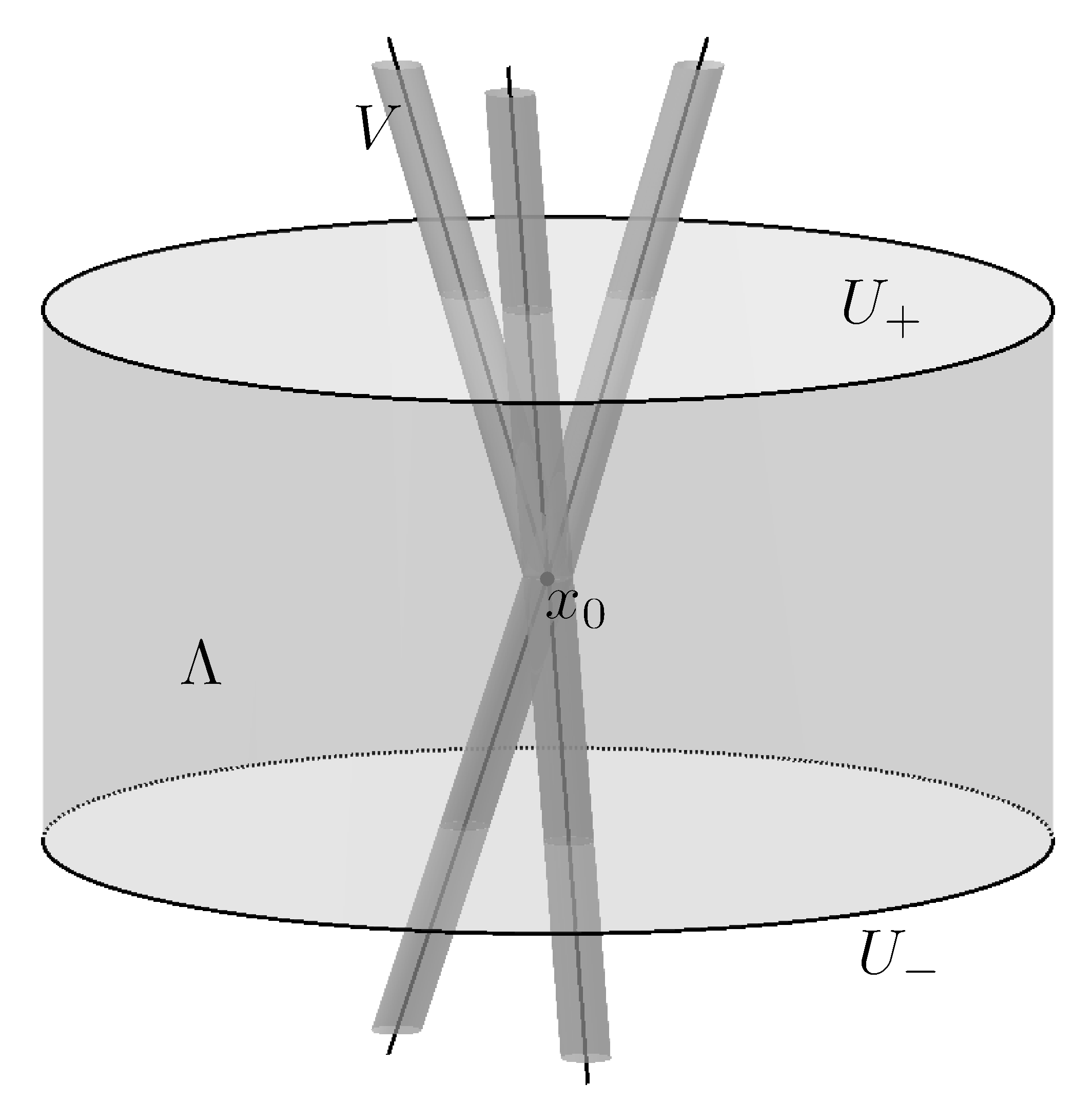
Figure 4: A branching point for the singular set $\mathscr{S}_{\mathrm{line}}$, surrounded by a cylinder $\Lambda$. The homotopy class of $Q_{0}$ restricted to the boundary of a disk which crosses transversely $\mathscr{S}_{\mathrm{line}}$ is determined by the number of intersections between the disk and $\mathscr{S}_{\mathrm{line}}$, modulo $2$. A configuration such as the one represented in this figure cannot occur, otherwise $Q_{0}$ restricted to $\partial U_{+}$ and $\partial U_{-}$ would be in different homotopy classes.

Remark 5.3.

For $k\in\{1,\,\ldots,\,q\}$, let $\nu^{(k)}$ be the direction vector associated with $L_{k}$ which has unit norm and points outward from $x_{0}$. Then, the stationarity of $\mathscr{S}_{\mathrm{line}}$ implies that

$$\sum_{k=1}^{q}\nu^{(k)}=0.$$

Indeed, taking an arbitrary vector field $\mathbf{X}$ supported in a small neighborhood of $x_{0}$, thanks to (5.2) we have

$$0=\kappa_{*}\sum_{k=1}^{q}\int_{0}^{\mathrm{length}(L_{k})}\nu^{(k)}_{i}\nu^{(k)}_{j}\frac{\partial\mathbf{X}_{i}}{\partial x_{j}}(x_{0}+t\nu^{(k)})\,\mathrm{d}t=-\kappa_{*}\sum_{k=1}^{q}\nu^{(k)}\cdot\mathbf{X}(x_{0}).$$

5.4 Concentration of the energy at the boundary: an example

The arguments we presented in this section may not be extended to the analysis of the singular set near the boundary of the domain. In particular, the stationarity of $\mu_{0}$ may fail. We discuss now an example where the boundary datum is independent of $\varepsilon$ and smooth, yet the geometry of the domain forces the energy of the minimizers to concentrate at the boundary. As a result, $\mathscr{S}_{\mathrm{line}}$ is non-empty but $\mathscr{S}_{\mathrm{line}}\subseteq\partial\Omega$, and $\mathscr{S}_{\mathrm{line}}$ is not a locally finite union of straight line segments.

Let $\mathbf{r}\colon(0,\,+\infty)\times\mathbb{R}\times[0,\,2\pi]\to\mathbb{R}^{3}$ be the cylindrical change of coordinates, given by

$$\mathbf{r}(\rho,\,z,\,\theta):=(\rho\cos\theta,\,\rho\sin\theta,\,z)^{\mathsf{T}}.$$

Let $D$ be the disk $B_{1}(2,0)$ in the $(\rho,\,z)$-plane, and let $\Omega$ be the solid torus generated by the revolution of $D$, that is

$$\Omega:=\mathbf{r}\left(D\times[0,\,2\pi)\right)=\left\{(x_{1},\,x_{2},\,x_{3})\in\mathbb{R}^{3}\colon\left(\sqrt{x_{1}^{2}+x_{2}^{2}}-2\right)^{2}+x_{3}^{2}<1\right\}.$$

We consider the boundary datum $g\in C^{1}(\partial\Omega,\,\mathscr{N})$ given by $g=h\circ\mathbf{r}^{-1}$, where

$$h(\rho,\,z):=s_{*}\left\{\left(\mathbf{e}_{1}\cos\frac{\varphi(\rho,\,z)}{2}+\mathbf{e}_{3}\sin\frac{\varphi(\rho,\,z)}{2}\right)^{\otimes 2}-\frac{1}{3}\operatorname{Id}\right\},$$

and $\varphi(\rho,\,z)$ is the oriented angle between the ray starting at $(2,\,0)$ and passing through $(\rho,\,z)$ and the positive $\rho$-axis. Notice that, for each $\theta\in[0,\,2\pi)$, the restriction of $g$ to the slice $\mathbf{r}(\partial D\times\{\theta\})$ has a non-trivial homotopy class. We will prove the following

Proposition 5.5.

For this choice of the domain and the boundary datum, we have

$$\mathscr{S}_{\mathrm{line}}=\mathbf{r}\left(\{(1,\,0)\}\times[0,\,2\pi)\right)=\left\{(x_{1},\,x_{2},\,x_{3})\in\mathbb{R}^{3}\colon x_{1}^{2}+x_{2}^{2}=1,\ x_{3}=0\right\}.$$

In particular, $\mathscr{S}_{\mathrm{line}}\subseteq\partial\Omega$.

Because of the cylindrical symmetry, the problem is essentially bidimensional. Indeed, given any map $Q\in H^{1}_{g}(\Omega,\,\mathbf{S}_{0})$, by a change of variable we obtain

(5.37) $$\begin{split}E_{\varepsilon}(Q,\,\Omega)&=\int_{0}^{2\pi}\int_{D}\left\{\frac{1}{2}\left|\partial_{\rho}(Q\circ\mathbf{r})\right|^{2}+\frac{1}{2}\left|\partial_{z}(Q\circ\mathbf{r})\right|^{2}+\frac{1}{\varepsilon^{2}}f(Q\circ\mathbf{r})\right\}\rho\,\mathrm{d}\rho\,\mathrm{d}z\,\mathrm{d}\theta\\ &\qquad+\int_{0}^{2\pi}\int_{D}\frac{1}{2\rho}\left|\partial_{\theta}(Q\circ\mathbf{r})\right|^{2}\,\mathrm{d}\rho\,\mathrm{d}z\,\mathrm{d}\theta.\end{split}$$

Therefore, a map $Q_{\varepsilon}$ is a minimizer for (LG_ε) in the class $H^{1}_{g}(\Omega,\,\mathbf{S}_{0})$ if and only if $Q_{\varepsilon}=P_{\varepsilon}\circ\mathbf{r}^{-1}$, where $P_{\varepsilon}$ only depend on $(\rho,\,z)$ and is a minimizer for the weighted functional

(5.38) $$F_{\varepsilon}(P,\,D):=2\pi\int_{D}\left\{\frac{1}{2}\left|\nabla P\right|^{2}+\frac{1}{\varepsilon^{2}}f(P)\right\}\rho\,\mathrm{d}\rho\mathrm{d}z$$

in the class

$$H^{1}_{h}(D,\,\mathbf{S}_{0}):=\left\{P\in H^{1}(D,\,\mathbf{S}_{0})\colon P=h\textrm{ on }\partial D\right\}.$$

Lemma 5.6.

For any $\delta>0$, there exists a constant $C_{\delta}$ such that, for any $0<\varepsilon<\delta/4$, there holds

$$F_{\varepsilon}(P_{\varepsilon},\,D)\leq 2\pi\kappa_{*}(1+\delta)|\log\varepsilon|+C_{\delta}.$$

Proof.

Fix $\delta>0$, $0<\varepsilon<\delta/4$ and let $\rho_{\delta}:=1+3\delta/4$, $D_{\delta}:=B^{2}_{\delta/4}(\rho_{\delta},\,0)$. We define a map $\tilde{P}_{\delta,\varepsilon}\colon D_{\delta}\to\mathbf{S}_{0}$ by setting

$$\tilde{P}_{\delta,\varepsilon}(\rho,\,z):=\eta_{\varepsilon}\left(\sqrt{(\rho-\rho_{\delta})^{2}+z^{2}}\right)h\left(2+\frac{4}{\delta}(\rho-\rho_{\delta}),\,\frac{4z}{\delta}\right)\qquad\textrm{if }(\rho-\rho_{\delta})^{2}+z^{2}\leq\frac{\delta^{2}}{16},$$

where $\eta_{\varepsilon}$ is defined by (3.5). The restriction of $\tilde{P}_{\delta,\varepsilon}$ to $\partial D_{\delta}$ is a $\mathscr{N}$-valued loop which depends on $\delta$ but not on $\varepsilon$, and has a non-trivial homotopy class. Therefore, there exists a map $\tilde{P}_{\delta}\colon D\setminus D_{\delta}\to\mathscr{N}$ such that

$$\tilde{P}_{\delta}=h\quad\textrm{on }\partial D,\qquad\tilde{P}_{\delta}=\tilde{P}_{\delta,\varepsilon}\quad\textrm{on }\partial D_{\delta}.$$

We extend $\tilde{P}_{\delta,\,\varepsilon}$ to a new map, still denoted $\tilde{P}_{\delta,\varepsilon}$, by setting $\tilde{P}_{\delta,\varepsilon}:=\tilde{P}_{\delta}$ on $D\setminus D_{\delta}$. Then $\tilde{P}_{\delta,\varepsilon}\in H^{1}_{h}(D,\,\mathbf{S}_{0})$ and, through a straightforward computation, we obtain

$$\begin{split}F_{\varepsilon}(P_{\varepsilon},\,D)&\leq F_{\varepsilon}(\tilde{P}_{\delta,\varepsilon},\,D)=F_{\varepsilon}(\tilde{P}_{\delta,\varepsilon},D_{\delta})+\pi\int_{D\setminus D_{\delta}}|\nabla\tilde{P}_{\delta}|^{2}\,\mathrm{d}\mathscr{H}^{2}\\ &\leq 2\pi(1+\delta)E_{\varepsilon}(\tilde{P}_{\delta,\varepsilon},D_{\delta})+C_{\delta}\\ &\leq 2\pi(1+\delta)\log\frac{\delta/4}{\varepsilon}+C_{\delta}=2\pi(1+\delta)|\log\varepsilon|+C_{\delta},\end{split}$$

where the symbol $C_{\delta}$ denotes several constants which only depend on $\delta$, $D$ and $h$. ∎

This lemma has an immediate consequence on the limit measure of the three-dimensional minimization problem.

Corollary 5.7.

There holds

$$\mu_{0}(\overline{\Omega})\leq 2\pi\kappa_{*}.$$

Proof.

Since we have $E_{\varepsilon}(Q_{\varepsilon},\,\Omega)=F_{\varepsilon}(P_{\varepsilon},\,D)$ because of (5.37), the corollary follows by taking the limit in Lemma 5.6 first as $\varepsilon\to 0$, then as $\delta\to 0$. ∎

Now, since the $3$D-minimizers $Q_{\varepsilon}$ satisfy $Q_{\varepsilon}=P_{\varepsilon}\circ\mathbf{r}^{-1}$ and $P_{\varepsilon}$ is independent of the $\theta$-variable, the singular set $\mathscr{S}_{\mathrm{line}}$ must be of the form $\mathscr{S}_{\mathrm{line}}=\mathbf{r}(\Sigma\times[0,\,2\pi))$ for some $\Sigma\subset\overline{D}$. Notice that $\Sigma$ is non-empty, because the homotopy class of the boundary datum $h$ is non-trivial. Moreover, $\Sigma$ is finite because $\mathscr{H}^{1}(\mathscr{S}_{\mathrm{line}})<\infty$.

Lemma 5.8.

Suppose that $(\rho_{0},\,z_{0})\in\Sigma$. Then

$$\mu_{0}(\overline{\Omega})\geq 2\pi\rho_{0}\kappa_{*}.$$

Combining Corollary 5.7 and Lemma 5.8, we immediately deduce that $\rho_{0}=1$, that is, $\Sigma=\{(1,\,0)\}$, whence Proposition 5.5 follows.

Proof of Lemma 5.8.

Fix a positive number $\delta<1/2$. It suffices to prove the inequality

(5.39) $$F_{\varepsilon}(P_{\varepsilon},\,D)\geq 2\pi\kappa_{*}(\rho_{0}-\delta)|\log\varepsilon|-C_{\delta}$$

for any small $\varepsilon$ and for some positive constant $C_{\delta}$ which depends only on $\delta$, $D$, $h$. The lemma will follow by using (5.37) and passing to the limit as $\varepsilon\to 0$, $\delta\to 0$.

Consider the disk $D^{\prime}:=B^{2}_{3/2}(2,\,0)\supset\!\supset D$, as well as the associated torus of revolution $\Omega^{\prime}:=\mathbf{r}(D^{\prime}\times[0,\,2\pi))$. We extend each minimizer $P_{\varepsilon}$ to a new map defined on $D^{\prime}$, still denoted by $P_{\varepsilon}$, by setting $P_{\varepsilon}:=h$ on $D^{\prime}\setminus D$. In the same way, we extend $Q_{\varepsilon}$ by setting $Q_{\varepsilon}:=g$ on $\Omega^{\prime}\setminus\Omega$. Moreover, we set

$$D^{\prime}_{\delta}:=B^{2}_{\delta/2}(\rho_{0},\,z_{0}).$$

Since $\Sigma$ is finite, reducing the value of $\delta$ if necessary we can assume that $D^{\prime}_{\delta}\cap\Sigma=\{(\rho_{0},\,z_{0})\}$. Therefore, Remark 5.2 implies that $Q_{\varepsilon}$ restricted to $\partial D^{\prime}_{\delta}$ has a non-trivial homotopy class, provided that $\varepsilon$ is small enough. Thus, we can apply Corollary 2.6 to bound from below the energy on $D^{\prime}_{\delta}$. We have

(5.40) $$\begin{split}F_{\varepsilon}(P_{\varepsilon},\,D^{\prime}_{\delta})&\geq 2\pi\left(\rho_{0}-\frac{\delta}{2}\right)E_{\varepsilon}(P_{\varepsilon},\,D^{\prime}_{\delta})\\ &\geq 2\pi\kappa_{*}\left(\rho_{0}-\frac{\delta}{2}\right)\,\phi_{0}(P_{\varepsilon},\,\partial D^{\prime}_{\delta})\,\log\frac{\delta}{\varepsilon}-C\bigg{(}E_{\varepsilon}(P_{\varepsilon},\,\partial D^{\prime}_{\delta})+1\bigg{)}.\end{split}$$

Thanks to Theorem 1 and Corollary 4.10, we have $Q_{\varepsilon}\to Q_{0}$ weakly in $H^{1}$, in a small neighborhood of $\mathbf{r}(\partial D^{\prime}_{\delta}\times[0,\,2\pi))\subset\Omega^{\prime}$. Therefore, modifying again the value of $\delta$ if necessary, we can assume that

$$Q_{\varepsilon}\rightharpoonup Q_{0}\qquad\textrm{weakly in }H^{1}(\mathbf{r}(\partial D^{\prime}_{\delta}\times[0,\,2\pi)),\,\mathbf{S}_{0})$$

(this property may not be satisfied for any value $\delta$, but it is satisfied for almost every value thanks to Fubini theorem). By Fubini theorem again and compact Sobolev embedding, this yields

$$P_{\varepsilon}\rightharpoonup P_{0}\qquad\textrm{weakly in }H^{1}(\partial D^{\prime}_{\delta},\,\mathbf{S}_{0})\textrm{ and uniformly,}$$

where $P_{0}:=Q_{0}\circ\mathbf{r}$ is an $\mathscr{N}$-valued map. In particular, there holds

(5.41) $$\phi_{0}(P_{\varepsilon},\,\partial D^{\prime}_{\delta})\to\phi_{0}(P_{0},\,\partial D^{\prime}_{\delta})=1\qquad\textrm{and}\qquad E_{\varepsilon}(P_{\varepsilon},\,\partial D^{\prime}_{\delta})\leq C_{\delta}.$$

Combining (5.40) and (5.41), we deduce that for (almost every) small enough $\delta$, there exist positive constants $C_{\delta}$ and  $\varepsilon_{\delta}$ such that (5.39) is satisfied for any $0<\varepsilon\leq\varepsilon_{\delta}$. This is enough to conclude the proof of the lemma. ∎

6 Sufficient conditions for (H)

6.1 Proof of Proposition 3

In this section, we analyze the role of the domain and the boundary data in connection with (H), and prove sufficient conditions for (H) to hold true. We prove first Proposition 3, namely, we assume that $\Omega$ is a bounded, Lipschitz domain and the boundary datum is bounded in $H^{1/2}(\partial\Omega,\,\mathscr{N})$, and we show that the inequalities

(6.1) $$\left\|Q_{\varepsilon}\right\|_{L^{\infty}(\Omega)}\leq M$$

and

(6.2) $$E_{\varepsilon}(Q_{\varepsilon})\leq M\left(\left|\log\varepsilon\right|+1\right)$$

are satisfied for some positive $M$. The $L^{\infty}$-bound (6.1) is easily obtained by a comparison argument.

Lemma 6.1.

Minimizers $Q_{\varepsilon}$ of (LG_ε) satisfy

$$\left\|Q_{\varepsilon}\right\|_{L^{\infty}(\Omega)}\leq\max\left\{\sqrt{\frac{2}{3}}s_{*},\,\left\|g_{\varepsilon}\right\|_{L^{\infty}(\partial\Omega)}\right\}.$$

Proof.

Set

$$M:=\max\left\{\sqrt{\frac{2}{3}}s_{*},\,\left\|Q_{\varepsilon}\right\|_{L^{\infty}(\partial\Omega)}\right\},$$

and define $\pi\colon\mathbf{S}_{0}\to\mathbf{S}_{0}$ by $\pi(Q):=M|Q|^{-1}Q$ if $|Q|\geq M$, $\pi(Q):=Q$ otherwise. We have

$$\mathrm{D}f(Q)\cdot Q=-a\left|Q\right|^{2}-b\operatorname{tr}Q^{3}+c\left|Q\right|^{4}>0\qquad\textrm{when }\left|Q\right|>\sqrt{\frac{2}{3}}s_{*}$$

(this follows from the inequality $\sqrt{6}|\operatorname{tr}Q^{3}|\leq|Q|^{3}$; see [50, Lemma 1]). We deduce that $f(\pi(Q))\geq f(Q)$ for any $Q$. Moreover, $\pi$ is the projection on a convex set, so it is $1$-Lipschitz continuous. Thus, the map $\pi\circ Q_{\varepsilon}$ belongs to $H^{1}_{g_{\varepsilon}}(\Omega,\,\mathbf{S}_{0})$, satisfies $|\nabla(\pi\circ Q_{\varepsilon})|\leq|\nabla Q_{\varepsilon}|$ a.e. and $E_{\varepsilon}(\pi\circ Q_{\varepsilon})\leq E_{\varepsilon}(Q_{\varepsilon})$, with strict inequality if $|Q_{\varepsilon}|>M$ on a set of positive measure. By minimality of $Q_{\varepsilon}$, we conclude that $|Q_{\varepsilon}|\leq M$ a.e. ∎

The logarithmic energy bound (6.2) is more delicate. The proof is adapted from an argument by Rivière [58, Proposition 2.1], which involves Hardt, Kinderlehrer and Lin’s re-projection trick (see [37, Lemma 2.3]) in an essential way.

Proof of Proposition 3.

Since the boundary data are supposed to be $\mathscr{N}$-valued, in particular they are bounded in $L^{\infty}$, therefore (6.1) follows by Lemma 6.1. We prove (6.2) by constructing a suitable comparison function, whose energy is bounded by the right-hand side of (6.2). For any $0<\varepsilon<1$, let $u_{\varepsilon}\in H^{1}(\Omega,\,\mathbf{S}_{0})$ be the harmonic extension of $g_{\varepsilon}$, i.e. the unique solution of

$$\begin{cases}-\Delta u_{\varepsilon}=0&\textrm{in }\Omega\\ u_{\varepsilon}=g_{\varepsilon}&\textrm{on }\partial\Omega.\end{cases}$$

Since $\{g_{\varepsilon}\}_{\varepsilon}$ is bounded in $H^{1/2}\cap L^{\infty}$, the sequence $\{u_{\varepsilon}\}_{\varepsilon}$ is bounded in $H^{1}\cap L^{\infty}$. Let $\delta>0$ be a small parameter to be chosen later. For any $A\in\mathbf{S}_{0}$ with $|A|\leq\delta$ and any $\varepsilon$, we define

$$u^{A}_{\varepsilon}:=\left(\eta_{\varepsilon}\circ\phi\right)\left(u_{\varepsilon}-A\right)\varrho\left(u_{\varepsilon}-A\right)$$

where $\phi\colon\mathbf{S}_{0}\to\mathbb{R}$ and $\varrho\colon\mathbf{S}_{0}\setminus\mathscr{C}\to\mathscr{N}$ are defined respectively in Lemmas 2.3, 2.2, and $\eta_{\varepsilon}\in C(\mathbb{R}^{+},\,\mathbb{R})$ is given by

$$\eta_{\varepsilon}(r):=\varepsilon^{-1}r\quad\textrm{if }0\leq r<\varepsilon,\qquad\eta_{\varepsilon}(r)=1\quad\textrm{if }r\geq\varepsilon.$$

By Lemma 2.2 and Corollary 2.8, we have $u^{A}_{\varepsilon}\in(H^{1}\cap L^{\infty})(\Omega,\,\mathbf{S}_{0})$. We differentiate $u^{A}_{\varepsilon}$ and, taking advantage of the Lipschitz continuity of $\phi$ (Lemma 2.3), we deduce

$$\left|\nabla u^{A}_{\varepsilon}\right|^{2}\leq C\left\{\left(\eta_{\varepsilon}^{\prime}\circ\phi\right)^{2}(u_{\varepsilon}-A)\left|\nabla u_{\varepsilon}\right|^{2}+\left(\eta_{\varepsilon}\circ\phi\right)^{2}(u_{\varepsilon}-A)\left|\nabla\left(\varrho(u_{\varepsilon}-A)\right)\right|^{2}\right\}.$$

We apply Corollary 2.8 to bound the derivative of $\varrho(u_{\varepsilon}-A)$:

$$\left|\nabla u^{A}_{\varepsilon}\right|^{2}\leq C\left\{\left(\eta_{\varepsilon}^{\prime}\circ\phi\right)^{2}(u_{\varepsilon}-A)+\frac{\left(\eta_{\varepsilon}\circ\phi\right)^{2}(u_{\varepsilon}-A)}{\phi^{2}(u_{\varepsilon}-A)}\right\}\left|\nabla u_{\varepsilon}\right|^{2}.$$

On the other hand, there holds

$$f\left(u^{A}_{\varepsilon}\right)\leq C\mathbbm{1}_{\{\phi(u_{\varepsilon}-A)\leq\varepsilon\}},$$

so

(6.3) $$E_{\varepsilon}\left(u^{A}_{\varepsilon}\right)\leq C\int_{\Omega}\left\{\left(\frac{\mathbbm{1}_{\{\phi(u_{\varepsilon}-A)\geq\varepsilon\}}}{\phi^{2}(u_{\varepsilon}-A)}+\varepsilon^{-2}\mathbbm{1}_{\{\phi(u_{\varepsilon}-A)\leq\varepsilon\}}\right)\left|\nabla u_{\varepsilon}\right|^{2}+\varepsilon^{-2}\mathbbm{1}_{\{\phi(u_{\varepsilon}-A)\leq\varepsilon\}}\right\}.$$

Now, fix a bounded subset $K\subseteq\mathbf{S}_{0}$, so large that $u_{\varepsilon}(x)+B_{\delta}^{\mathbf{S}_{0}}\subseteq K$ for a.e. $x\in\Omega$ and any $\varepsilon$ (we denote by $B_{\delta}^{\mathbf{S}_{0}}$ the set of $Q\in\mathbf{S}_{0}$ with $|Q|\leq\delta$). We set $K_{\varepsilon}:=K\cap\{\phi\leq\varepsilon\}$. We integrate (6.3) with respect to $A\in B^{\mathbf{S}_{0}}_{\delta}$. We apply Fubini-Tonelli theorem and introduce the new variable $B:=u_{\varepsilon}(x)-A$. We obtain

$$\begin{split}\int_{B_{\delta}^{\mathbf{S}_{0}}}E_{\varepsilon}\left(u^{A}_{\varepsilon}\right)\,\mathrm{d}\mathscr{H}^{5}(A)\leq C\int_{\Omega}\left\{\left(\int_{K\setminus K_{\varepsilon}}\frac{\mathrm{d}\mathscr{H}^{5}(B)}{\phi^{2}(B)}+\varepsilon^{-2}\mathscr{H}^{5}(K_{\varepsilon})\right)\left|\nabla u_{\varepsilon}\right|^{2}+\varepsilon^{-2}\mathscr{H}^{5}(K_{\varepsilon})\right\}\,\mathrm{d}x.\end{split}$$

We claim that

(6.4) $$\mathscr{H}^{5}(K_{\varepsilon})\leq C\varepsilon^{2}\qquad\textrm{and}\qquad\int_{K\setminus K_{\varepsilon}}\frac{\mathrm{d}\mathscr{H}^{5}(B)}{\phi^{2}(B)}\leq C\left(|\log\varepsilon|+1\right).$$

To simplify the presentation, we postpone the proof of this claim. With the help of (6.4), we obtain

$$\int_{B^{5}_{\delta}}E_{\varepsilon}\left(u^{A}_{\varepsilon}\right)\,\mathrm{d}\mathscr{H}^{5}(A)\leq C\left\{\left(|\log\varepsilon|+1\right)\left\|\nabla u_{\varepsilon}\right\|^{2}_{L^{2}(\Omega)}+1\right\}\leq C\left(|\log\varepsilon|+1\right).$$

Therefore, we can choose $A_{0}\in\mathbf{S}_{0}$ such that $|A_{0}|\leq\delta$ and

(6.5) $$E_{\varepsilon}\left(u^{A_{0}}_{\varepsilon}\right)\leq C\left(|\log\varepsilon|+1\right).$$

The map $u^{A_{0}}_{\varepsilon}$ satisfies the desired energy estimate, but it does not satisfy the boundary condition, since

(6.6) $$u^{A_{0}}_{\varepsilon}=\varrho\left(g_{\varepsilon}-A_{0}\right)\qquad\textrm{on }\partial\Omega.$$

To correct this, we consider the maps $\{\varrho_{A}\}_{A\in B_{\delta}^{\mathbf{S}_{0}}}$ defined by

$$\varrho_{A}\colon Q\in\mathscr{N}\mapsto\varrho(Q-A).$$

This is a continuous family of mappings in $C^{1}(\mathscr{N},\,\mathscr{N})$ and $\varrho_{0}=\operatorname{Id}_{\mathscr{N}}$. Therefore, we can choose $\delta$ so small that the map $\varrho_{A}\colon\mathscr{N}\to\mathscr{N}$ is a diffeomorphism for any $A\in B_{\delta}^{\mathbf{S}_{0}}$ (in particular for $A=A_{0}$). Let $\mathscr{U}$ be the set defined by

$$\mathscr{U}:=\left\{\lambda Q\colon\lambda\in\mathbb{R}^{+},\ Q\in\mathscr{N}\right\}.$$

We extend $\varrho_{A_{0}}^{-1}$ to a Lipschitz function $\mathscr{F}\colon\mathscr{U}\to\mathscr{U}$ by setting

$$\mathscr{F}(\lambda Q):=\lambda\varrho_{A_{0}}^{-1}(Q)\qquad\textrm{for any }\lambda\in\mathbb{R}^{+},\ Q\in\mathscr{N}.$$

Remark that any $P\in\mathscr{U}\setminus\{0\}$ can be uniquely written in the form $P=\lambda Q$ for $\lambda\in\mathbb{R}^{+}$ and $Q\in\mathscr{N}$, so $\mathscr{F}$ is well-defined. Also, $f\circ\mathscr{F}(P)=f(P)$ because $\mathscr{F}(P)$ and $P$ have the same scalar invariants. The map $P_{\varepsilon}:=\mathscr{F}\circ u^{A_{0}}_{\varepsilon}$ is well-defined, because $u^{A_{0}}_{\varepsilon}\in\mathscr{U}$. Moreover, $P_{\varepsilon}$ belongs to $H^{1}_{g_{\varepsilon}}(\Omega,\,\mathbf{S}_{0})$ thanks to (6.6), and satisfies

$$E_{\varepsilon}(P_{\varepsilon})\leq C\left(|\log\varepsilon|+1\right)$$

due to (6.5). By comparison, the minimizers satisfy (6.2). ∎

The claim (6.4) follows by this

Lemma 6.2.

For any $R>0$, there exist positive constants $C_{R},\,M_{R}$ such that, for any non increasing, non negative function $g\colon\mathbb{R}^{+}\to\mathbb{R}^{+}$, there holds

$$\int_{B_{R}^{\mathbf{S}_{0}}}\left(g\circ\phi\right)(Q)\,\mathrm{d}\mathscr{H}^{5}(Q)\leq C_{R}\int_{0}^{M_{R}}\left(s+s^{4}\right)g(s)\,\mathrm{d}s.$$

Assuming that the lemma holds true, choose $R$ so large that $K\subseteq B_{R}^{\mathbf{S}_{0}}$. Then, the two assertions of Claim (6.4) follow by taking $g=\mathbbm{1}_{(0,\,\varepsilon)}$ and $g(s)=\varepsilon^{-2}\mathbbm{1}_{(0,\,\varepsilon)}(s)+s^{-2}\mathbbm{1}_{[\varepsilon,\,+\infty)}(s)$, respectively. For the sake of clarity, we split the proof of Lemma 6.2 into a few steps. For $r>0$, we let $\operatorname{dist}_{r}$ denote the geodesic distance in $\partial B_{r}^{\mathbf{S}_{0}}$, that is

(6.7) $$\operatorname{dist}_{r}(Q,\,A):=\inf\left\{\int_{0}^{1}\left|\gamma^{\prime}(t)\right|\,\mathrm{d}t\colon\gamma\in C^{1}([0,\,1],\,\partial B_{1}^{\mathbf{S}_{0}}),\ \gamma(0)=Q,\ \gamma(1)\in A\right\}$$

for any $Q\in\partial B_{r}^{\mathbf{S}_{0}}$ and $A\subseteq\partial B_{r}^{\mathbf{S}_{0}}$, and set $\mathscr{N}^{\prime}_{r}:=\mathscr{C}\cap\partial B_{r}^{\mathbf{S}_{0}}$. Notice that there exists a positive constant $C$ such that

(6.8) $$\operatorname{dist}_{|Q|}(Q,\,P)\leq C\left|Q-P\right|$$

for any $Q$, $P\in\mathbf{S}_{0}$ with $|Q|=|P|$.

Lemma 6.3.

There exists a positive constant $\alpha$ such that

$$\phi(Q)\geq\alpha\operatorname{dist}_{|Q|}\left(Q,\,\mathscr{N}^{\prime}_{|Q|}\right)\qquad\textrm{for any }Q\in\mathbf{S}_{0}.$$

Proof.

Fix $Q\in\mathbf{S}_{0}$ and $P\in\mathscr{N}^{\prime}_{|Q|}$. By Lemmas 2.1 and 2.2, we can write

$$Q=s\left(\mathbf{n}^{\otimes 2}-\frac{1}{3}\operatorname{Id}\right)+sr\left(\mathbf{m}^{\otimes 2}-\frac{1}{3}\operatorname{Id}\right)\qquad\textrm{and}\qquad P=-s^{\prime}\left(\mathbf{p}^{\otimes 2}-\frac{1}{3}\operatorname{Id}\right),$$

for some orthonormal pair $(\mathbf{n},\,\mathbf{m})$, some unit vector $\mathbf{p}$, $s$, some positive numbers $s$, $s^{\prime}$ and $0\leq r\leq 1$. Through simple algebra, we obtain

(6.9) $$\left|Q-P\right|^{2}=\frac{2}{3}s^{2}\left(r^{2}-r+1\right)-\frac{2}{3}ss^{\prime}(1-r)+\frac{2}{3}{s^{\prime}}^{2}+2ss^{\prime}\left\{(\mathbf{n}\cdot\mathbf{p})^{2}+r(\mathbf{m}\cdot\mathbf{p})^{2}\right\}.$$

By setting $s^{\prime}=0$ and $s=0$ in this identity, we see that $|P|=|Q|$ if and only if

(6.10) $${s^{\prime}}^{2}=s^{2}\left(r^{2}-r+1\right).$$

By minimizing (with respect to $s^{\prime}$, $\mathbf{p}$) the right-hand side in (6.9), subject to the constraint (6.10), we find

$$\begin{split}\operatorname{dist}^{2}(Q,\,\mathscr{N}^{\prime}_{1})=\frac{2}{3}s^{2}\sqrt{r^{2}-r+1}\left\{(1-r)^{2}-\left(\sqrt{r^{2}-r+1}-1\right)^{2}\right\}\leq\frac{2}{3}s^{2}(1-r)^{2}=\frac{2}{3}s_{*}^{2}\phi^{2}(Q).\end{split}$$

Combining this inequality with (6.8), the lemma follows. ∎

Lemma 6.4.

Let ${\mathscr{N}^{\prime}}$ be a compact $n$-submanifold of a smooth Riemann $m$-manifold $\mathscr{M}$, and let

$$U_{\delta}:=\left\{x\in\mathscr{M}\colon\operatorname{dist}_{\mathscr{M}}(x,\,\mathscr{N}^{\prime})\leq\delta\right\}$$

be the $\delta$-neighborhood of $\mathscr{N}^{\prime}$ in $\mathscr{M}$, for $\delta>0$ (here $\operatorname{dist}_{\mathscr{M}}$ stands for the geodesic distance in $\mathscr{M}$). There exist $\delta_{*}>0$ and, for any $\delta\in(0,\,\delta_{*})$, a constant $C=C(\mathscr{M},\,\mathscr{N}^{\prime},\delta)>0$ such that for any decreasing function $h\colon\mathbb{R}^{+}\to\mathbb{R}^{+}$ there holds

$$\int_{U_{\delta}}h\left(\operatorname{dist}_{\mathscr{M}}(x,\,\mathscr{N}^{\prime})\right)\,\mathrm{d}\mathscr{H}^{m}(x)\leq C\int_{0}^{C\delta}s^{m-n-1}h(s)\,\mathrm{d}s.$$

Proof.

We identify $\mathbb{R}^{m}=\mathbb{R}^{n}\times\mathbb{R}^{m-n}$, and call the variable $y=(y^{\prime},\,z)\in\mathbb{R}^{n}\times\mathbb{R}^{m-n}$. For a small $\delta_{*}>0$, the $\delta_{*}$-neighborhood $U_{\delta_{*}}$ can be covered with finitely many open sets $\{V_{j}\}_{1\leq j\leq K}$ and, for each $j$, there exists a bilipschitz homeomorphism $\varphi_{j}\colon V_{j}\to W_{j}\subseteq\mathbb{R}^{m}$ which maps $\mathscr{N}^{\prime}\cap V_{j}$ onto $\mathbb{R}^{n}\cap W_{j}$. Due to the bilipschitz continuity of the $\varphi_{j}$’s, there exist two constants $\gamma_{1}$, $\gamma_{2}$ such that, for any $j$ and any $y=(y^{\prime},\,z)\in W_{j}$, there holds

$$\gamma_{1}\left|z\right|\leq\operatorname{dist}_{\mathscr{M}}(\varphi_{j}^{-1}(y),\,\mathscr{N})\leq\gamma_{2}\left|z\right|.$$

Therefore, if $0<\delta<\delta_{*}$ the change of variable $x=\varphi_{j}^{-1}(y)$ implies

$$\begin{split}\int_{U_{\delta}}h\left(\operatorname{dist}_{\mathscr{M}}(x,\,\mathscr{N}^{\prime})\right)\,\mathrm{d}\mathscr{H}^{m}(x)&\leq\sum_{j=1}^{K}\int_{\varphi^{-1}_{j}(V_{j})}h\left(\gamma_{1}|z|\right)\,\left|\mathrm{J}\varphi_{j}^{-1}(y)\right|\,\mathrm{d}\mathscr{H}^{m}(y)\\ &\leq M\int_{B^{m-n}(0,\,\gamma_{2}\delta)}h(\gamma_{1}|z|)\,\mathrm{d}\mathscr{H}^{m-n}(z)\end{split}$$

where $M$ is an upper bound for the norm of the Jacobians $\mathrm{J}\varphi_{j}^{-1}$. Then, passing to polar coordinates,

$$\begin{split}\int_{U_{\delta}}h\left(\operatorname{dist}_{\mathscr{M}}(x,\,\mathscr{N}^{\prime})\right)\,\mathrm{d}\mathscr{H}^{m}(x)&\leq M\int_{0}^{\gamma_{2}\delta}\rho^{m-n-1}h(\gamma_{1}\rho)\,\mathrm{d}\rho\\ &\leq M\gamma_{1}^{1+n-m}\int_{0}^{\gamma_{1}\gamma_{2}\rho}s^{m-n-1}h(s)\,\mathrm{d}s.\qed\end{split}$$

Proof of Lemma 6.2.

By Lemma 2.3, the function $\phi$ is positively homogeneous of degree $1$. Then,

$$\int_{B_{R}^{\mathbf{S}_{0}}}(g\circ\phi)(Q)\,\mathrm{d}\mathscr{H}^{5}(Q)=\int_{0}^{R}\rho^{4}\int_{\partial B_{1}^{\mathbf{S}_{0}}}g\left(\rho\phi(Q)\right)\,\mathrm{d}\mathscr{H}^{4}(Q)\,\mathrm{d}\rho.$$

By applying Lemma 6.3, and since $g$ is a decreasing function,

$$\int_{B_{R}^{\mathbf{S}_{0}}}(g\circ\phi)(Q)\,\mathrm{d}\mathscr{H}^{5}(Q)\leq\int_{0}^{R}\rho^{4}\int_{\partial B_{1}^{\mathbf{S}_{0}}}g\left(\alpha\rho\operatorname{dist}_{1}(Q,\,\mathscr{N}^{\prime}_{1})\right)\,\mathrm{d}\mathscr{H}^{4}(Q)\,\mathrm{d}\rho.$$

Now, we apply Lemma 6.4 with $\mathscr{M}=\partial B_{1}^{\mathbf{S}_{0}}$, $\mathscr{N}^{\prime}=\mathscr{N}^{\prime}_{1}$ and $h\colon s\mapsto g(\alpha\rho s)$. We find constants $\delta$ and $C$ such that, letting $U_{\delta}$ be the $\delta$-neighborhood of $\mathscr{N}^{\prime}_{1}$ in $\partial B_{1}^{\mathbf{S}_{0}}$ and $V_{\delta}:=\partial B_{1}^{\mathbf{S}_{0}}\setminus U_{\delta}$, we have

$$\begin{split}\int_{B_{R}^{\mathbf{S}_{0}}}&(g\circ\phi)(Q)\,\mathrm{d}\mathscr{H}^{5}(Q)\\ &=\int_{0}^{R}\rho^{4}\left\{\int_{U_{\delta}}g\left(\alpha\rho\operatorname{dist}_{1}(Q,\,\mathscr{N}^{\prime}_{1})\right)\,\mathrm{d}\mathscr{H}^{4}(Q)+\int_{V_{\delta}}g\left(\alpha\rho\operatorname{dist}_{1}(Q,\,\mathscr{N}^{\prime}_{1})\right)\,\mathrm{d}\mathscr{H}^{4}(Q)\right\}\,\mathrm{d}\rho\\ &\leq C\int_{0}^{R}\rho^{4}\left\{\int_{0}^{C\delta}sg(\alpha\rho s)\,\mathrm{d}s+g(\alpha\rho\delta)\,\mathscr{H}^{4}(V_{\delta})\right\}\,\mathrm{d}\rho\end{split}$$

(to bound the integral on $V_{\delta}$, we use again that $g$ is decreasing). Now, the two terms can be easily handled by changing the variables and using Fubini-Tonelli theorem:

$$\begin{split}\int_{B_{R}^{\mathbf{S}_{0}}}(g\circ\phi)(Q)\,\mathrm{d}\mathscr{H}^{5}(Q)&\leq\alpha^{-2}C\int_{0}^{R}\rho^{2}\int_{0}^{\alpha\rho\delta C}tg(t)\,\mathrm{d}t\,\mathrm{d}\rho+(\alpha\delta)^{-5}C\mathscr{H}^{4}(V_{\delta})\int_{0}^{\alpha\delta R}t^{4}g(t)\,\mathrm{d}t\\ &\leq C_{\alpha,\delta,R}\int_{0}^{C_{\alpha,\delta,R}}\left(t+t^{4}\right)g(t)\,\mathrm{d}t.\end{split}$$

Since $\alpha$, $\delta$ depend only on $\phi$ and $\mathscr{N}^{\prime}_{1}$, the lemma is proved. ∎

6.2 Proof of Propositions 4 and 5

Condition (H) may be satisfied even if the boundary datum is not $\mathscr{N}$-valued. As we show in this section, if the doman satisfies a topological condition (H₂) and if boundary datum is smooth (at least $H^{1}\cap L^{\infty}$), satisfying a uniform $L^{\infty}$-bound and a logarithmic energy estimate (H₃), then (6.1)–(6.2) are satisfied for some constant $M=M(\Omega,\,M_{0})>0$. This proves Proposition 4. We remark that (H₂) is a technical assumption which is needed in the proof, and we have not investigated whether it is necessary for (H). At the end of the section, we also prove Proposition 5.

Once again, the $L^{\infty}$-bound (6.1) follows immediately from (H₃) and Lemma 6.1. Next, we prove (6.2) by constructing an admissible comparison function whose energy is controlled by the right-hand side of (6.2). If $\Omega$ is a ball, it sufficies to extend homogeneously the boundary data. Since $\Omega$ is bilipschitz equivalent to a handlebody by (H₂), we reduce to the case of a ball by cutting each handle of $\Omega$ along a meridian disk. This technique was used already in [37, Lemma 1.1]. In the following lemma, we construct cut disks with suitable properties.

Lemma 6.5.

Assume that (H₂) and (H₃) hold. There exists a finite number of properly embedded disks $D_{1},\,D_{2},\ldots,\,D_{k}\subseteq\Omega$ such that $\Omega\setminus\cup_{i=1}^{k}D_{i}$ is diffeomorphic to a ball,

(6.11) $$E_{\varepsilon}(g_{\varepsilon},\,\partial D_{i})\leq C\left(\left|\log{\varepsilon}\right|+1\right)$$

and

(6.12) $$\operatorname{dist}(g_{\varepsilon}(x),\,\mathscr{N})\to 0\qquad\textrm{uniformly in }x\in\bigcup_{i=1}^{k}\partial D_{i}.$$

Proof.

For each handle $i$ of $\Omega$, there is an open set $U_{i}$ such that $\partial\Omega\cap U_{i}$ is foliated by

$$\partial\Omega\cap U_{i}=\coprod_{-a_{0}<a<a_{0}}\partial D_{i}^{a},$$

where the generic $D_{i}^{a}$ is a properly embedded disk, which cross transversely a generator of $\pi_{1}(\Omega)$ at some point. Then, Fatou’s lemma implies that

$$\int_{-a_{0}}^{a_{0}}\liminf_{\varepsilon\to 0}E_{\varepsilon}(g_{\varepsilon},\,{\partial D_{i}^{a}})\,\mathrm{d}a\leq\liminf_{\varepsilon\to 0}\int_{-a_{0}}^{a_{0}}E_{\varepsilon}(g_{\varepsilon},\,{\partial D_{i}^{a}})\,\mathrm{d}a\stackrel{{\scriptstyle\eqref{hp:bd data}}}{{\leq}}C\left(\left|\log\varepsilon\right|+1\right),$$

so, by an average argument, we can choose the parameter $a$ in such a way that $D_{i}:=D^{a}_{i}$ satisfies (6.11). Then, (6.12) is obtained by the same arguments as Lemma 3.12. (As in the lemma, we apply Sobolev embedding inequality not on $\partial D_{i}$ directly, but on $1$-cells $K\subseteq\partial D_{i}$ of size comparable to $\varepsilon^{\alpha}\left|\log\varepsilon\right|$.) Furthermore, by construction $\Omega\setminus\cup_{i=1}^{k}D_{i}$ is a ball, since we have removed a meridian disk for each handle of $\Omega$. ∎

Proof of Proposition 4.

The $L^{\infty}$-bound (6.1) holds by virtue of Lemma 6.1, so we only need to prove (6.2). Assume for a moment that $\Omega=B_{1}$. In this case, define the function

(6.13) $$P_{\varepsilon}(x):=g_{\varepsilon}\left(\frac{x}{|x|}\right)\qquad\textrm{for }x\in B_{1}.$$

Then $P_{\varepsilon}\in H^{1}_{g_{\varepsilon}}(B_{1},\,\mathbf{S}_{0})$ and we easily compute

$$\begin{split}E_{\varepsilon}(P_{\varepsilon})=\int_{0}^{1}\int_{\partial B_{1}}\left(\left|\nabla_{\top}g_{\varepsilon}\right|^{2}+\varepsilon^{-2}\rho^{2}f(g_{\varepsilon})\right)\,\mathrm{d}\mathscr{H}^{2}\,\mathrm{d}\rho\stackrel{{\scriptstyle\eqref{hp:bd data}}}{{\leq}}C\left(\left|\log\varepsilon\right|+1\right),\end{split}$$

so the lemma holds true when $\Omega=B_{1}$.

Now, arguing as in [37, Lemma 1.1], we prove that the general case can be reduced to the previous one. Let $\Omega$ be any domain satisfying (H₂), and let $D_{1},\,\ldots,\,D_{k}$ be the disks given by Lemma 6.5. By (6.12), there exists $\varepsilon_{0}>0$ such that, for any $0<\varepsilon\leq\varepsilon_{0}$ and any $x\in\cup_{i}\partial D_{i}$,

$$\operatorname{dist}(g_{\varepsilon}(x),\,\mathscr{N})\leq\delta_{0}.$$

For ease of notation, for a fixed $i\in\{1,\,\ldots,\,k\}$ we assume, up to a bilipschitz equivalence, that $D_{i}=B_{1}^{2}$. Then, we define $\hat{g}_{\varepsilon,i}\colon B^{2}_{1}\to\mathbf{S}_{0}$ by

$$\hat{g}_{\varepsilon,i}\left(x\right):=\begin{cases}\dfrac{\delta_{0}+\left|x\right|-1}{\delta_{0}}g_{\varepsilon}\left(\dfrac{x}{|x|}\right)+\dfrac{1-\left|x\right|}{\delta_{0}}(\varrho\circ g_{\varepsilon})\left(\dfrac{x}{|x|}\right)&\textrm{if }1-\delta_{0}\leq\left|x\right|\leq 1\\ v_{\varepsilon}\left(\dfrac{x}{1-\delta_{0}}\right)&\textrm{if }\left|x\right|\leq 1-\delta_{0},\end{cases}$$

where $v_{\varepsilon}\in H^{1}(B^{2}_{1},\,\mathbf{S}_{0})$ is the extension of ${\varrho\circ g_{\varepsilon}}_{|\partial B^{2}_{1}}$ given by Lemma 3.3. By a straightforward computation, one checks that

(6.14) $$E_{\varepsilon}(\hat{g}_{\varepsilon,i},\,D_{i})\leq C\left(E_{\varepsilon}(g_{\varepsilon},\,\partial D_{i})+\left|\log\varepsilon\right|+1\right).$$

Now, consider two copies $D_{i}^{+}$ and $D^{-}_{i}$ of each disk $D_{i}$. Let $\Omega^{\prime}$ be a smooth domain such that

$$\Omega^{\prime}\simeq\left(\Omega\setminus\cup_{i}D_{i}\right)\cup_{i}D_{i}^{+}\cup_{i}D^{-}_{i},$$

and let $\varphi\colon\Omega^{\prime}\to\Omega$ be the smooth map which identifies each $D^{+}_{i}$ with the corresponding $D_{i}^{-}$ (see Figure 5). This new domain is simply connected, and in fact is diffeomorphic to a ball. Up to a bilipschitz equivalence, we will assume that $\Omega^{\prime}$ is a ball. We define a boundary datum $g_{\varepsilon}^{\prime}$ for $\Omega^{\prime}$ by setting $g_{\varepsilon}^{\prime}:=g_{\varepsilon}$ on $\Omega\setminus\cup_{i}D_{i}$, and $g_{\varepsilon}^{\prime}:=g_{\varepsilon,\,i}$ on $D_{i}^{+}\cup D_{i}^{-}$. Then, (6.14), (6.11) and (H₃) imply

$$E_{\varepsilon}(g_{\varepsilon}^{\prime},\,\partial\Omega)\leq C\left(E_{\varepsilon}(g_{\varepsilon},\,\partial\Omega)+\left|\log\varepsilon\right|+1\right)\leq C\left(\left|\log\varepsilon\right|+1\right).$$

Then Formula (6.13) gives a map $P_{\varepsilon}^{\prime}\in H^{1}_{g_{\varepsilon}^{\prime}}(\Omega^{\prime},\,\mathbf{S}_{0})$ which satisfies

$$E_{\varepsilon}(P^{\prime}_{\varepsilon},\,\Omega^{\prime})\leq C\left(\left|\log\varepsilon\right|+1\right).$$

Since ${P^{\prime}_{\varepsilon}}_{|D_{i}^{+}}={P^{\prime}_{\varepsilon}}_{|D_{i}^{-}}$ for every $i$, the map $P^{\prime}_{\varepsilon}$ factorizes through $\varphi$, and defines a new function $P_{\varepsilon}\in H^{1}_{g_{\varepsilon}}(\Omega,\,\mathbf{S}_{0})$ such that

$$E_{\varepsilon}(P_{\varepsilon},\,\Omega)\leq C\left(\left|\log\varepsilon\right|+1\right).$$

By comparison, we conclude that (6.2) holds for any $0<\varepsilon\leq\varepsilon_{0}$. Now, fix $\varepsilon_{0}<\varepsilon<1$ and consider the ($\mathbf{S}_{0}$-valued) harmonic extension $\tilde{P}_{\varepsilon}$ of $g_{\varepsilon}$. There holds

$$\|\nabla\tilde{P}_{\varepsilon}\|^{2}_{L^{2}(\Omega)}\leq C\left\|\nabla g_{\varepsilon}\right\|^{2}_{L^{2}(\partial\Omega)}\stackrel{{\scriptstyle\eqref{hp:bd data}}}{{\leq}}C\left(\left|\log\varepsilon\right|+1\right),\qquad\|\tilde{P}_{\varepsilon}\|^{2}_{L^{\infty}(\Omega)}\leq C\left\|g_{\varepsilon}\right\|^{2}_{L^{\infty}(\partial\Omega)}\stackrel{{\scriptstyle\eqref{hp:bd data}}}{{\leq}}C$$

and so

$$E_{\varepsilon}(P_{\varepsilon})\leq\frac{1}{2}\|\nabla\tilde{P}_{\varepsilon}\|^{2}_{L^{2}(\Omega)}+C\varepsilon_{0}^{-2}\leq C\left(1+\varepsilon_{0}^{2}\right)\left(\left|\log\varepsilon\right|+1\right).$$

Also in this case, the lemma follows by comparison. ∎

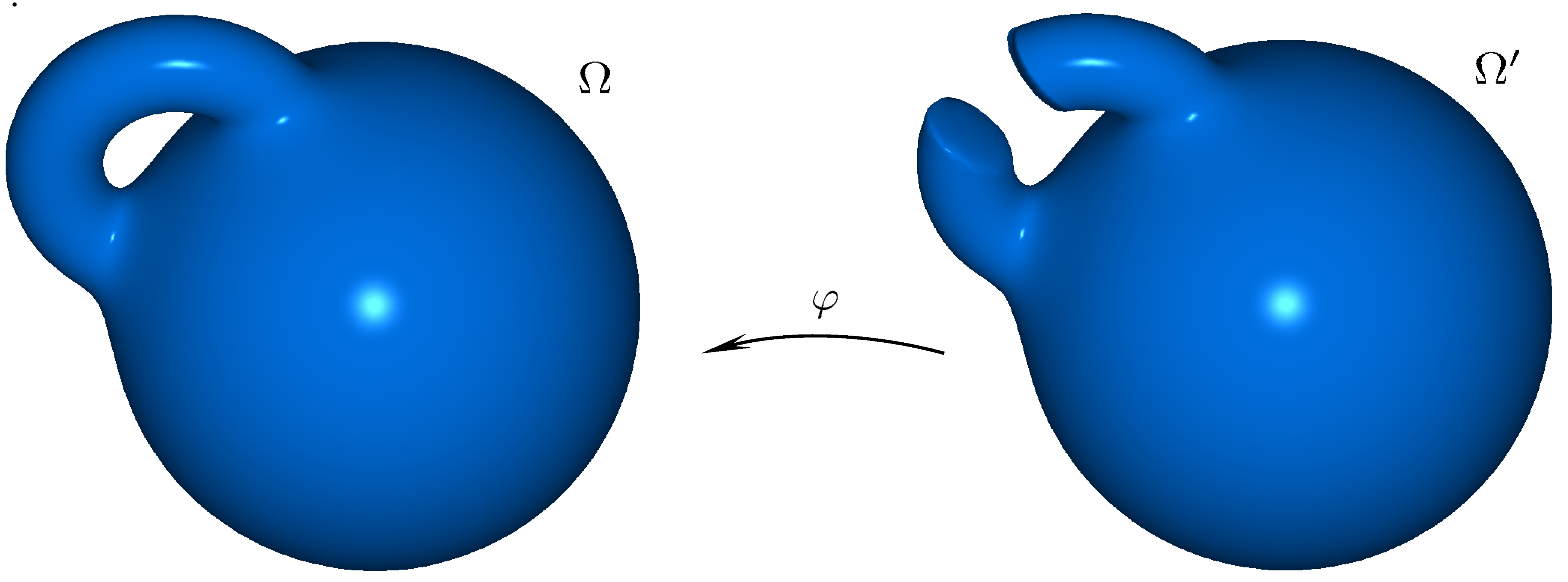
Figure 5: On the left, a ball with one handle. On the right, the corresponding domain $\Omega^{\prime}$: the handle has been cut along a disk. The map $\varphi\colon\Omega^{\prime}\to\Omega$ identifies the opposite disks in the handle cut.

We turn now to the proof of Proposition 5. The boundary data we construct are smooth approximations of a map $\partial\Omega\to\mathscr{N}$ with at least one point singularity. Then, the lower bound for the energy follows by the estimates of Subsection 2.2.

Proof of Proposition 5.

Up to rotations and translations, we can assume that the $x_{3}$-axis $\{x_{1}=x_{2}=0\}$ crosses transversely $\partial\Omega$ at one point $x_{0}$ at least. Let $\eta_{\varepsilon}\in C^{\infty}(\mathbb{R}^{+},\,\mathbb{R})$ be a cut-off function satisfying

$$\eta_{\varepsilon}(0)=\eta_{\varepsilon}^{\prime}(0)=0,\qquad\eta_{\varepsilon}(r)=s_{*}\textrm{ for }r\geq\varepsilon,\qquad 0\leq\eta_{\varepsilon}\leq s_{*},\qquad\left|\eta_{\varepsilon}^{\prime}\right|\leq C\varepsilon^{-1}.$$

Set

$$g_{\varepsilon}(x):=\eta_{\varepsilon}(|x^{\prime}|)\left\{\left(\frac{x^{\prime}}{|x^{\prime}|}\right)^{\otimes 2}-\frac{1}{3}\operatorname{Id}\right\}\qquad\textrm{for }x\in\partial\Omega,$$

where $x^{\prime}:=(x_{1},\,x_{2},\,0)$. Computing as in Lemma 3.3, one sees that $\{g_{\varepsilon}\}$ satisfies (H₃). It remains to prove that the energy of minimizers $Q_{\varepsilon}$ satisfies a logarithmic lower bound. Take a ball $B_{r}(x_{0})$. If the radius $r$ is small enough, the set $\Omega\cap B_{r}(x_{0})$ can be mapped diffeomorphically onto the half-ball

$$U:=\left\{x\in\mathbb{R}^{3}\colon\left|x\right|\leq 1,\ x_{3}\geq 0\right\},$$

so we can assume WLOG that $\Omega\cap B_{r}(x_{0})=U$. Let $U_{s}:=\{x\in U\colon x_{3}=s\}$, for $r/2\leq s\leq r$. The map ${Q_{\varepsilon}}_{|\partial U_{s}}\colon\partial U_{s}\to\mathscr{N}$ is a homotopically non-trivial loop, which satisfies $E_{\varepsilon}(Q_{\varepsilon},\,\partial U_{s})\leq C$. Then, by applying Corollary 2.6 we deduce

$$E_{\varepsilon}(Q_{\varepsilon},\,U_{s})\geq\kappa_{*}\log\frac{s}{\varepsilon}-C$$

for a constant $C$ depending on $r$, $\Omega$. By integrating this bound for $s\in(r/2,\,r)$, the proposition follows. ∎

7 Coexistence of line and point singularities: an example

In this section, we show through an example that both the set of line singularities $\mathscr{S}_{\mathrm{line}}$ and the set of point singularities $\mathscr{S}_{\mathrm{pts}}$ may be non-empty. We consider the following domain. For two fixed positive numbers

(7.1) $$L>0\qquad\textrm{and}\qquad 0<r<\frac{1}{2},$$

define

$$p_{\pm}:=(\pm(L+1),\,0,\,0),\qquad\Omega_{\pm}:=B_{1}(p_{\pm}),\qquad\Omega_{0}:=\left([-L-1,\,L+1]\times B^{2}_{r}(0)\right)\setminus\left(\Omega_{-}\cup\Omega_{+}\right)$$

and $\Omega:=\Omega_{-}\cup\Omega_{0}\cup\Omega_{+}$. In other words, the domain consists of two balls joined by a cylinder about the $x_{1}$-axis (see Figure 1). This is a Lipschitz domain; however, one could consider a smooth domain $\Omega^{\prime}$, obtained from $\Omega$ by “smoothing the corners”, and the results of this section could be easily adapted to $\Omega^{\prime}$.

We write $\partial\Omega=\Gamma_{-}\cup\Gamma_{0}\cup\Gamma_{+}$, where $\Gamma_{\pm}:=\partial\Omega_{\pm}\setminus\Omega_{0}$ and $\Gamma_{0}:=\partial\Omega_{0}\setminus(\overline{\Omega}_{+}\cup\overline{\Omega}_{-})$. We define the auxiliary functions $\chi\in H^{1}(0,\,2\pi)$, $\eta_{\varepsilon}\in H^{1}(0,\,\pi)$ and $\xi_{r}\in H^{1}(0,\,\pi)$ by

$$\chi(\theta):=\begin{cases}{\pi}/{2}-{3\theta}/{5}&\textrm{for }0\leq\theta\leq 5\pi/6\\ 0&\textrm{for }5\pi/6<\theta<7\pi/6\\ {7\pi}/{10}-{3\theta}/{5}&\textrm{for }7\pi/6\leq\theta\leq 2\pi,\end{cases}\qquad\eta_{\varepsilon}(\varphi):=\begin{cases}\varepsilon^{-1}\varphi&\textrm{for }0\leq\varphi\leq\varepsilon\\ 1&\textrm{for }\varepsilon<\varphi<\pi-\varepsilon\\ \varepsilon^{-1}(\pi-\varphi)&\textrm{for }\pi-\varepsilon\leq\varphi\leq\pi\end{cases}$$

and

$$\xi_{r}(\tilde{\varphi}):=\begin{cases}0&\textrm{if }0\leq\tilde{\varphi}\leq\arcsin r\\ \dfrac{\arcsin 2r\left(\tilde{\varphi}-\arcsin r\right)}{\arcsin 2r-\arcsin r}&\textrm{if }\arcsin 2r<\tilde{\varphi}<\arcsin 2r\\ \tilde{\varphi}&\textrm{if }\arcsin 2r\leq\tilde{\varphi}\leq\pi.\end{cases}$$

Notice that

(7.2) $$\left|\eta_{\varepsilon}^{\prime}\right|\leq\varepsilon^{-1}\qquad\textrm{and}\qquad\left|\xi_{r}^{\prime}\right|\leq 2.$$

The boundary datum $g_{\varepsilon}$ is defined as follows. We parametrize $\Gamma_{+}$ using spherical coordinates $(\theta,\,\varphi)\in[0,\,2\pi]\times[0,\,\pi]$ centered at $p_{+}$:

$$x_{1}=L+1+\sin\varphi\cos\theta,\qquad x_{2}=\sin\varphi\sin\theta,\qquad x_{3}=\cos\varphi$$

and define $g_{\varepsilon}$ on $\Gamma_{+}$ by

(7.3) $$g_{\varepsilon}\colon(x_{1},\,x_{2},\,x_{3})\in\Gamma_{+}\mapsto s_{*}\eta_{\varepsilon}(\varphi)\left\{\bigg{(}\mathbf{e}_{1}\cos\chi(\theta)+\mathbf{e}_{2}\sin\chi(\theta)\bigg{)}^{\otimes 2}-\frac{1}{3}\operatorname{Id}\right\}.$$

On $\Gamma_{-}$, we use spherical coordinates about the $x_{1}$-axis, i.e. $(\tilde{\theta},\,\tilde{\varphi})\in[0,\,2\pi]\times[0,\,\pi]$ given by

$$x_{1}=-L-1+\cos\tilde{\varphi},\qquad x_{2}=\sin\tilde{\varphi}\cos\tilde{\theta},\qquad x_{3}=\sin\tilde{\varphi}\sin\tilde{\theta}$$

and set

(7.4) $$g_{\varepsilon}\colon(x_{1},\,x_{2},\,x_{3})\in\Gamma_{-}\mapsto s_{*}\left\{\left(\mathbf{e}_{1}\cos\xi_{r}(\tilde{\varphi})+\mathbf{e}_{2}\sin\xi_{r}(\tilde{\varphi})\cos\tilde{\theta}+\mathbf{e}_{3}\sin\xi_{r}(\tilde{\varphi})\sin\tilde{\theta}\right)^{\otimes 2}-\frac{1}{3}\operatorname{Id}\right\}.$$

Finally, we set

$$g_{\varepsilon}:=s_{*}\left(\mathbf{e}_{1}^{\otimes 2}-\frac{1}{3}\operatorname{Id}\right)\qquad\textrm{on }\Gamma_{0}.$$

This defines a map $g_{\varepsilon}\in H^{1}(\partial\Omega,\,\mathbf{S}_{0})$ which is non-orientable with two point singularities on $\Gamma_{+}$, is constant on $\Gamma_{0}$ and has a hedgehog-type behaviour on $\Gamma_{-}$. In Figure 1, we represent the direction of the eigenvector associated with the leading eigenvalue of $g_{\varepsilon}(x)$, for $x\in\partial\Omega$. Of course, one could regularize the functions $\chi$, $\eta_{\varepsilon}$ and $\xi_{r}$ so that the map $g_{\varepsilon}$ is smooth; this would not affect our arguments. As usual, pick a subsequence $\varepsilon_{n}$ so that the measures $\mu_{\varepsilon_{n}}$ defined by (4.17) converge weakly^⋆ in $C(\overline{\Omega})^{\prime}$ to a measure $\mu_{0}$, and let $\mathscr{S}_{\mathrm{line}}\subseteq\overline{\Omega}$ be the support of $\mu_{0}$. Let $\mathscr{S}_{\mathrm{pts}}\subseteq\Omega\setminus\mathscr{S}_{\mathrm{line}}$ be a set such that the sequence $\{Q_{\varepsilon_{n}}\}_{n\in\mathbb{N}}$ is compact in $C^{0}(\Omega\setminus(\mathscr{S}_{\mathrm{line}}\cup\mathscr{S}_{\mathrm{pts}}),\,\mathbf{S}_{0})$. By Theorem 1, such a set exists and is locally finite in $\Omega\setminus\mathscr{S}_{\mathrm{line}}$. We will show the following result, which implies Proposition 6.

Proposition 7.1.

There exists $L^{*}$ such that, if

$$L\geq L^{*}$$

then $\emptyset\neq\mathscr{S}_{\mathrm{line}}\subseteq\left\{x_{1}\geq 0\right\}$ and $\mathscr{S}_{\mathrm{pts}}\cap\{x_{1}\leq-L/2\}\neq\emptyset$.

Remark 7.1.

The presence of a point defect is not forced by a topological obstruction. In other words, there exists maps $P_{\varepsilon}\colon\Omega\to\mathbf{S}_{0}$ which satisfy $P_{\varepsilon}=g_{\varepsilon}$ on $\partial\Omega$ and converge to a map with a line singularity but no point singularity. Indeed, let $\varphi\colon\overline{\Omega}\to\overline{B}_{1}$ be a bilipschitz homeomorphism such that $\varphi(L,\,0,\,\pm 1)=(0,\,0,\,\pm 1)$. Then, the functions

$$P_{\varepsilon}(x):=g_{\varepsilon}\circ\varphi^{-1}\left(\frac{\varphi(x)}{\left|\varphi(x)\right|}\right)$$

converge a.e. to a map with a line singularity $\mathscr{S}_{\mathrm{line}}:=\varphi^{-1}\left\{x_{1}=x_{2}=0\right\}$, but no point singularities. The convergence also holds in $H^{1}_{\mathrm{loc}}(\Omega\setminus\mathscr{S}_{\mathrm{line}},\,\mathbf{S}_{0})$.

We split the proof of Proposition 7.1 into some lemmas. Throughout the section, we use the symbol $C$ to denote a generic constant, which does not depend on $\varepsilon$, $L$ and $r$.

Lemma 7.2.

There exists a constant $M$, independent of $L$ and $r$, such that

$$E_{\varepsilon}(Q_{\varepsilon},\,\Omega)\leq M\left(\left|\log\varepsilon\right|+1\right)\qquad\textrm{and}\qquad\left\|Q_{\varepsilon}\right\|_{L^{\infty}(\Omega)}\leq M$$

for any $0<\varepsilon<1$.

Proof.

The $L^{\infty}$-bound follows by Lemma 6.1, since $|g_{\varepsilon}(x)|\leq(2/3)^{1/2}s_{*}$ for a.e. $x\in\partial\Omega$ and any $0<\varepsilon<1$. The energy bound follows by a comparison argument. We define a map $P_{\varepsilon}$ on $\Omega_{+}$ and $\Omega_{-}$ by homogeneous extension:

$$P_{\varepsilon}(x):=g_{\varepsilon}\left(p_{+}+\frac{x-p_{+}}{\left|x-p_{+}\right|}\right)\ \textrm{ if }x\in\Omega_{+},\qquad P_{\varepsilon}(x):=g_{\varepsilon}\left(p_{-}+\frac{x-p_{-}}{\left|x-p_{-}\right|}\right)\ \textrm{ if }x\in\Omega_{-},$$

whereas we set

$$P_{\varepsilon}(x):=s_{*}\left(\mathbf{e}_{1}^{\otimes 2}-\frac{1}{3}\operatorname{Id}\right)\ \textrm{ if }x\in\Omega_{0}.$$

(Here we assume that $g_{\varepsilon}$ is defined also on $\partial\Omega_{\pm}\setminus\Gamma_{\pm}$, by the same formulae (7.3)–(7.4).) Then, the map $P_{\varepsilon}$ is continuous and belongs to $H^{1}(\Omega,\,\mathbf{S}_{0})$. Moreover, $E_{\varepsilon}(P_{\varepsilon},\,\Omega_{0})=0$ since ${P_{\varepsilon}}_{|\Omega_{0}}$ is constant and takes values in $\mathscr{N}$. A simple computation, based on (7.2), concludes the proof. ∎

For any $s\in\mathbb{R}$, let $U_{s}:=\Omega\cap\{x_{1}<s\}$ and $G_{\varepsilon}(s):=E_{\varepsilon}(Q_{\varepsilon},\,U_{s})$. Fubini-Tonelli theorem entails that $G_{\varepsilon}^{\prime}(s)=E_{\varepsilon}(Q_{\varepsilon},\,\Omega\cap\{x_{1}=s\})$ for a.e. $s$.

Lemma 7.3.

There exist positive constants $L_{*}$ and $M$ such that, for any $L\geq L_{*}$ and any $0<\varepsilon\leq 1/2$, there holds

$$G_{\varepsilon}(0)\leq M.$$

In particular, if $L\geq L_{*}$ then $\mathscr{S}_{\mathrm{line}}\subseteq\overline{\Omega}\setminus U_{0}$.

Proof.

This proof is based on the same arguments as Proposition 7. Define the set

$$D^{\varepsilon}:=\left\{s\in(0,\,L)\colon G^{\prime}_{\varepsilon}(s)\leq\frac{2M}{L}\left(\left|\log\varepsilon\right|+1\right)\right\}.$$

By Lemma 7.2 and an average argument, we know that

(7.5) $$\mathscr{H}^{1}(D^{\varepsilon})\geq\frac{L}{2}.$$

Moreover, there exists $L_{*}>0$ such that, for any $L\geq L_{*}$, any $0<\varepsilon\leq 1/2$ and any $s\in D^{\varepsilon}$, there holds

$$G^{\prime}_{\varepsilon}(s)\leq\eta_{0}\left|\log\varepsilon\right|$$

where $\eta_{0}$ is the constant given by Proposition 3.8. Therefore, for a fixed $s\in D^{\varepsilon}$ we can apply Proposition 3.8 to the map $u_{\varepsilon}:={Q_{\varepsilon}}_{|\{s\}\times B^{2}_{r}}$. Notice that $u_{\varepsilon}$ is defined on a disk, whereas the maps we consider in Proposition 3.8 are defined over a sphere. However, since $u_{\varepsilon}$ takes a constant value on the boundary, it can be identified with a map defined on a sphere by collapsing $\{s\}\times\partial B^{2}_{r}$ into a point. Setting $h(\varepsilon):=\varepsilon^{1/2}|\log\varepsilon|$ and $A_{\varepsilon}:=(s-h(\varepsilon),\,s)\times B^{2}_{r}$, we find maps $v_{\varepsilon}\colon\{s-h(\varepsilon)\}\times B^{2}_{r}\to\mathscr{N}$ and $\varphi_{\varepsilon}\colon A_{\varepsilon}\to\mathbf{S}_{0}$ such that

(7.6) $$\frac{1}{2}\int_{\{s-h(\varepsilon)\}\times B_{r}^{2}}\left|\nabla v_{\varepsilon}\right|^{2}\,\mathrm{d}\mathscr{H}^{2}\leq G^{\prime}_{\varepsilon}(s),\qquad E_{\varepsilon}(\varphi_{\varepsilon})\leq Ch(\varepsilon)\left|\log\varepsilon\right|.$$

Now, consider the set $V_{s}:=[s-h(\varepsilon)-r,\,s-h(\varepsilon)]\times B^{2}_{r}$ (we assume that $L_{*}>2$, so that $s-h(\varepsilon)-r>-L$ for $\varepsilon\leq 1/2$) and the map $\tilde{v}_{\varepsilon}\in H^{1}(\partial V_{s},\,\mathscr{N})$ given by $\tilde{v}_{\varepsilon}:=v_{\varepsilon}$ on $\{s\}\times B^{2}_{r}$,

$$\tilde{v}_{\varepsilon}:=s_{*}\left(\mathbf{e}_{1}^{\otimes 2}-\frac{1}{3}\operatorname{Id}\right)\qquad\textrm{on }\partial V_{s}\setminus\left(\{s\}\times B^{2}_{r}\right).$$

Thanks to (7.6), we have

$$\frac{1}{2}\int_{\partial V_{s}}\left|\nabla\tilde{v}_{\varepsilon}\right|^{2}\,\mathrm{d}\mathscr{H}^{2}=\frac{1}{2}\int_{\{s\}\times B^{2}_{r}}\left|\nabla v_{\varepsilon}\right|^{2}\,\mathrm{d}\mathscr{H}^{2}\leq G^{\prime}_{\varepsilon}(s).$$

Then, by applying Lemma 3.1 (which is possible because $V_{s}$ is bilipschitz equivalent to a ball), we find a map $w_{\varepsilon}\in H^{1}(V_{s},\,\mathscr{N})$ such that $w_{\varepsilon}=\tilde{v}_{\varepsilon}$ on $\partial V_{s}$ and

(7.7) $$\frac{1}{2}\int_{V_{s}}\left|\nabla w_{\varepsilon}\right|^{2}\leq CG^{\prime}_{\varepsilon}(s)^{1/2},$$

for a constant $C$ independent of $\varepsilon$, $L$, $r$. (Here we have used that $r<1$.) Finally, we define a map $\tilde{w}_{\varepsilon}\in H^{1}(U_{s},\,\mathbf{S}_{0})$ as follows. We set $\tilde{w}_{\varepsilon}:=\varphi_{\varepsilon}$ on $[s-h(\varepsilon),\,s]\times B^{2}_{r}$ and $\tilde{w}_{\varepsilon}:=w_{\varepsilon}$ on $V_{s}$,

$$\tilde{w}_{\varepsilon}:=s_{*}\left(\mathbf{e}_{1}^{\otimes 2}-\frac{1}{3}\operatorname{Id}\right)\qquad\textrm{on }\Omega_{0}\setminus\left([s-h(\varepsilon)-r,\,s]\times B^{2}_{r}\right)$$

and use an homogeneous extension to construct $\tilde{w}_{\varepsilon}$ on $\Omega_{-}$:

$$\tilde{w}_{\varepsilon}(x):=g_{\varepsilon}\left(p_{-}+\frac{x-p_{-}}{\left|x-p_{-}\right|}\right)\qquad\textrm{for }x\in\Omega_{-}.$$

The map $\tilde{w}_{\varepsilon}$ is continuous, satisfies $E_{\varepsilon}(\tilde{w}_{\varepsilon})=0$ on $\Omega_{0}\setminus([s-h(\varepsilon)-r,\,s]\times B^{2}_{r})$ and $E_{\varepsilon}(\tilde{w}_{\varepsilon},\,\Omega_{-})\leq C$ because of (7.2). Thus, from (7.6) and (7.7) we infer

$$E_{\varepsilon}(\tilde{w}_{\varepsilon},\,U_{s})\leq CG^{\prime}_{\varepsilon}(s)^{1/2}+C.$$

Moreover, $\tilde{w}_{\varepsilon}$ is an admissible competitor for $Q_{\varepsilon}$, because $\tilde{w}_{\varepsilon}=Q_{\varepsilon}$ on $\partial U_{s}$. Then, the minimality of $Q_{\varepsilon}$ yields

(7.8) $$G_{\varepsilon}(s)\leq CG^{\prime}_{\varepsilon}(s)^{1/2}+C\qquad\textrm{for a.e. }s\in D^{\varepsilon}\textrm{ and every }0<\varepsilon\leq\frac{1}{2}.$$

Thanks to (7.5) and (7.8), we apply Lemma 4.2 to $y:=G_{\varepsilon}$ and obtain

$$G_{\varepsilon}(0)\leq\left(1+\frac{2}{L}\right)C\leq\left(1+\frac{2}{L_{*}}\right)C=:M$$

for every $0<\varepsilon\leq 1/2$. Therefore, $\mu_{\varepsilon}\mathbin{\vrule height=6.88889pt,depth=0.0pt,width=0.55974pt\vrule height=0.55974pt,depth=0.0pt,width=5.59721pt}U_{0}\to 0$ in $\mathscr{M}_{\mathrm{b}}(U_{0}):=C_{0}(U_{0})^{\prime}$ and hence $\mathscr{S}_{\mathrm{line}}\subseteq\overline{\Omega}\setminus U_{0}$. ∎

Before concluding the proof of Proposition 7.1, we recall a well-known fact. Given $r>0$ and a continuous maps $\mathbf{n}\colon B^{2}_{r}\to\mathbb{S}^{2}$ which take a constant value on $\partial B^{2}_{r}$, it is possible to define the topological degree of $\mathbf{n}$. Indeed, the topological space which is obtained by collapsing the boundary of $\partial B^{2}_{r}$ into a point is homeomorphic to a sphere. Then, since $\mathbf{n}_{|\partial B^{2}_{r}}$ is a constant, $\mathbf{n}$ induces a continuous map $\mathbb{S}^{2}\to\mathbb{S}^{2}$ whose homotopy class is characterized by an integer number $d$ called the degree of $\mathbf{n}$. We will write $d=:\deg(\mathbf{n},\,B^{2}_{r})$. In case $\mathbf{n}\in H^{1}(B^{2}_{r},\,\mathbb{S}^{2})$ takes a constant value at the boundary, the degree of $\mathbf{n}$ can still be defined (for instance, one can apply the VMO-theory by Brezis and Nirenberg [19, 20]).

Lemma 7.4.

For any $r>0$ and any $\mathbf{n}\in H^{1}(B_{r}^{2},\,\mathbb{S}^{2})$ with constant value at the boundary, if

$$\frac{1}{2}\int_{B^{2}_{r}}\left|\nabla\mathbf{n}\right|^{2}\,\mathrm{d}\mathscr{H}^{2}<4\pi$$

then $\deg(\mathbf{n},\,B^{2}_{r})=0$.

Proof.

By applying the area formula, we obtain

$$\int_{B^{2}_{r}}\left|\partial_{x_{1}}\mathbf{n}\times\partial_{x_{2}}\mathbf{n}\right|\,\mathrm{d}\mathscr{H}^{2}=\int_{\mathbf{n}(B^{2}_{r})}\mathscr{H}^{0}\left(\mathbf{n}^{-1}(y)\right)\,\mathrm{d}\mathscr{H}^{2}(y)\geq\mathscr{H}^{2}\left(\mathbf{n}(B^{2}_{r})\right).$$

On the other hand, we have $|\partial_{x_{1}}\mathbf{n}\times\partial_{x_{2}}\mathbf{n}|\leq|\partial_{x_{1}}\mathbf{n}||\partial_{x_{2}}\mathbf{n}|\leq|\nabla\mathbf{n}|^{2}/2$. Therefore, there holds

$$\frac{1}{2}\int_{B^{2}_{r}}\left|\nabla\mathbf{n}\right|^{2}\,\mathrm{d}\mathscr{H}^{2}\geq\mathscr{H}^{2}\left(\mathbf{n}(B^{2}_{r})\right).$$

If the left-hand side is $<4\pi$, then $\mathbf{n}$ is not surjective and so $\deg(\mathbf{n},\,B^{2}_{r})=0$ (see e.g. [19, Property 1]). ∎

Proof of Proposition 7.1.

Arguing as in the proof of Proposition 5, and using that the boundary conditions ${g_{\varepsilon}}_{|U_{+}}$ are non orientable, one shows that

$$E_{\varepsilon}(Q_{\varepsilon})\geq C\left(\left|\log\varepsilon\right|-1\right)$$

for any $\varepsilon$, $L$ and $r$, so $\mathscr{S}_{\mathrm{line}}\neq\emptyset$. By Lemma 7.3, there exists $L_{*}$ such that $\mathscr{S}_{\mathrm{line}}\subseteq\Omega\setminus U_{0}$ if $L\geq L_{*}$. Set

(7.9) $$L^{*}:=\max\left\{L_{*},\,\frac{M}{\pi s_{*}}\right\}$$

where $M$ is given by Lemma 7.3, and let $L\geq L^{*}$. The proposition follows once we show that $\mathscr{S}_{\mathrm{pts}}\cap U_{-L/2}\neq\emptyset$.

By applying Lemma 7.3, Theorem 1 and Corollary 4.10, we deduce that $Q_{\varepsilon_{n}}\to Q_{0}$ in $H^{1}(U_{-\delta},\,\mathbf{S}_{0})$ for every $\delta>0$, where $Q_{0}\colon U_{0}\to\mathscr{N}$ is a locally minimizing harmonic map. Passing to the limit as $\varepsilon\to 0$ in Lemma 7.3, we see that

(7.10) $$\frac{1}{2}\int_{U_{0}}\left|\nabla Q_{0}\right|^{2}\leq M$$

for an $L$-independent constant $M$. In particular, $Q_{0}\in H^{1}(U_{0},\,\mathscr{N})$. An average argument, combined with Lemma 7.10, shows that there exists $-L<s<-L/2$ such that $Q_{0}\in H^{1}(\{s\}\times B^{2}_{r},\,\mathscr{N})$ and

$$\frac{1}{2}\int_{\{s\}\times B^{2}_{r}}\left|\nabla Q_{0}\right|^{2}\,\mathrm{d}\mathscr{H}^{2}\leq\frac{4M}{L}.$$

Due to Lemma 3.6, we find a lifting of ${Q_{0}}_{|\partial U_{s}}$, i.e. a map $\mathbf{n}_{0}\in H^{1}(\partial U_{s},\,\mathbb{S}^{2})$ which satisfies (3.1) and $|\nabla Q_{0}|^{2}=2s_{*}|\nabla\mathbf{n}_{0}|^{2}$ a.e. Then, we have

(7.11) $$\frac{1}{2}\int_{\{s\}\times B^{2}_{r}}\left|\nabla\mathbf{n}_{0}\right|^{2}\,\mathrm{d}\mathscr{H}^{2}\leq\frac{2M}{s_{*}L}.$$

Combining (7.11) with (7.9), we deduce

$$\frac{1}{2}\int_{\{s\}\times B^{2}_{r}}\left|\nabla\mathbf{n}_{0}\right|^{2}\,\mathrm{d}\mathscr{H}^{2}\leq 2\pi.$$

Moreover, $\mathbf{n}_{0}$ takes a constant value on the boundary of $\{s\}\times B^{2}_{r}$, since $Q_{0}$ does. Then, by Lemma 7.4, $\deg(\mathbf{n}_{0},\{s\}\times B^{2}_{r})=0$. On the other hand, $\deg(\mathbf{n}_{0},\,\partial U_{s}\cap\Gamma_{0})=0$ since $\mathbf{n}_{0}$ takes a constant value on $\partial U_{s}\cap\Gamma_{0}$, and $\deg(\mathbf{n}_{0},\,\Gamma_{-})$ can be computed explicitly thanks to (7.4). This yields

$$\deg(\mathbf{n}_{0},\,\partial U_{s})=\deg(\mathbf{n}_{0},\,\Gamma_{-})=\pm 1,$$

so the map ${Q_{0}}_{|\partial U_{s}}$ is homotopically non-trivial and $\mathscr{S}_{\mathrm{pts}}\cap U_{s}\neq\emptyset$. ∎

Acknowledgements. Most of this work has been carried out while the author was a PhD student at Sorbonne Universités, UPMC — Université Paris 6, CNRS, UMR 7598, Laboratoire Jacques-Louis Lions. Part of the research leading to these results has received funding from the European Research Council under the European Union’s Seventh Framework Programme (FP7/2007-2013) / ERC grant agreement n° 291053. The author would like to thank his Ph.D. advisor, professor Fabrice Bethuel, as well as professor Sir John Ball FRS, for constant support and helpful advice. He is also very grateful to professor Giandomenico Orlandi, doctor Arghir Zarnescu, Mark Wilkinson and Xavier Lamy for inspiring conversations and interesting remarks.

Conflict of Interest. The authors declare that they have no conflict of interest.

References

- [1] G. Alberti, S. Baldo, and G. Orlandi. Variational convergence for functionals of Ginzburg-Landau type. Indiana Univ. Math. J., 54(5):1411–1472, 2005.
- [2] W. K. Allard. On the first variation of a varifold. Ann. Math. (2), 95:417–491, 1972.
- [3] W. K. Allard and F. J. Almgren, Jr. The structure of stationary one dimensional varifolds with positive density. Invent. Math., 34(2):83–97, 1976.
- [4] F. J. Almgren Jr. Plateau’s Problem: An invitation to varifold geometry. W. A. Benjamin, Inc., New York-Amsterdam, 1966.
- [5] L. Ambrosio and H. M. Soner. Level set approach to mean curvature flow in arbitrary codimension. J. Differential Geom., 43(4):693–737, 1996.
- [6] L. Ambrosio and E. G. Virga. A boundary value problem for nematic liquid crystals with a variable degree of orientation. Arch. Rational Mech. Anal., 114(4):335–347, 1991.
- [7] K. E. Atkinson. An Introduction to Numerical Analysis. John Wiley & Sons, Inc., New York, second edition, 1989.
- [8] J. M. Ball and A. Majumdar. Nematic liquid crystals: from Maier–Saupe to a continuum theory. Mol. Cryst. and Liq. Cryst., 525(1):1–11, 2010.
- [9] J. M. Ball and A. Zarnescu. Orientability and energy minimization in liquid crystal models. Arch. Rational Mech. Anal., 202(2):493–535, 2011.
- [10] F. Bethuel, H. Brezis, and F. Hélein. Asymptotics for the minimization of a Ginzburg-Landau functional. Cal. Var. Partial Differential Equations, 1(2):123–148, 1993.
- [11] F. Bethuel, H. Brezis, and F. Hélein. Ginzburg-Landau Vortices. Progress in Nonlinear Differential Equations and their Applications, 13. Birkhäuser Boston Inc., Boston, MA, 1994.
- [12] F. Bethuel, H. Brezis, and G. Orlandi. Asymptotics for the Ginzburg-Landau equation in arbitrary dimensions. J. Funct. Anal., 186(2):432–520, 2001.
- [13] F. Bethuel and D. Chiron. Some questions related to the lifting problem in Sobolev spaces. Contemporary Mathematics, 446:125–152, 2007.
- [14] F. Bethuel, G. Orlandi, and D. Smets. Approximations with vorticity bounds for the Ginzburg-Landau functional. Commun. Contemp. Math., 6(5):803–832, 2004.
- [15] F. Bethuel and X. Zheng. Density of smooth functions between two manifolds in Sobolev spaces. J. Funct. Anal., 80(1):60 – 75, 1988.
- [16] J. Bourgain, H. Brezis, and P. Mironescu. Lifting in Sobolev spaces. Journal d’Analyse Mathématique, 80(1):37–86, 2000.
- [17] H. Brezis, J.-M. Coron, and E. H. Lieb. Harmonic maps with defects. Comm. Math. Phys., 107(4):649–705, 1986.
- [18] H. Brezis and P. Mironescu. Sur une conjecture de E. De Giorgi relative à l’énergie de Ginzburg-Landau. C. R. Acad. Sci. Paris Sér. I Math., 319(2):167–170, 1994.
- [19] H. Brezis and L. Nirenberg. Degree theory and BMO. I. Compact manifolds without boundaries. Selecta Math. (N.S.), 1(2):197–263, 1995.
- [20] H. Brezis and L. Nirenberg. Degree theory and BMO. II. Compact manifolds with boundaries. Selecta Math. (N.S.), 2(3):309–368, 1996. With an appendix by the authors and Petru Mironescu.
- [21] G. Canevari. Biaxiality in the asymptotic analysis of a 2D Landau-de Gennes model for liquid crystals. ESAIM : Control, Optimisation and Calculus of Variations, 21(1):101–137, 2015.
- [22] S. Chandrasekhar and G. S. Ranganath. The structure and energetics of defects in liquid crystals. Adv. Phys., 35(6):507–596, 1986.
- [23] D. Chiron. Étude mathématique de modèles issus de la physique de la matière condensée. PhD thesis, Université Pierre et Marie Curie–Paris 6, 2004.
- [24] P.E. Cladis and M. Kléman. Non-singular disclinations of strength in nematics. J. Phys. France, 33(5–6):591–598, 1972.
- [25] A. Contreras and X. Lamy. Biaxial escape in nematics at low temperature. Preprint arXiv: 1405.2055, 2014.
- [26] T. A. Davis and E. C. Gartland Jr. Finite element analysis of the Landau-de Gennes minimization problem for liquid crystals. SIAM J. on Numer. Anal., 35(1):336–362, 1998.
- [27] P. G. De Gennes and J. Prost. The Physics of Liquid Crystals. International series of monographs on physics. Clarendon Press, 1993.
- [28] G. Di Fratta, J. M. Robbins, V. Slastikov, and A. Zarnescu. Half-integer point defects in the -tensor theory of nematic liquid crystals. J. Nonlinear Sci., pages 1–20, 2015.
- [29] J. L. Ericksen. Liquid crystals with variable degree of orientation. Arch. Rational Mech. Anal., 113(2):97–120, 1991.
- [30] H. Federer. Geometric measure theory. Die Grundlehren der mathematischen Wissenschaften, Band 153. Springer-Verlag New York Inc., New York, 1969.
- [31] F. C. Frank. On the theory of liquid crystals. Discuss. Faraday Soc., 25:19–28, 1958.
- [32] G. Friedel. Les états mésomorphes de la matière. Annals of Physics, 18:273–474, 1922. Translated by T. J. Sluckin, D. A. Dunmur and H. Stegemeyer in “Crystals That Flow: Classic Papers from the History of Liquid Crystals”, Taylor and Francis, 2004.
- [33] E. C. Gartland Jr and S. Mkaddem. Instability of radial hedgehog configurations in nematic liquid crystals under Landau–de Gennes free-energy models. Phys. Rev. E, 59(1):563–567, 1999.
- [34] M. Giaquinta and E. Giusti. The singular set of the minima of certain quadratic functionals. Ann. Sc. Norm. Super. Pisa Cl. Sci., 11(1):45–55, 1984.
- [35] D. Golovaty and J. A. Montero. On minimizers of a Landau-de Gennes energy functional on planar domains. Arch. Rational Mech. Anal., 213(2):447–490, 2014.
- [36] E. F. Gramsbergen, L. Longa, and W. H. de Jeu. Landau theory of the nematic-isotropic phase transition. Physics Reports, 135(4):195–257, April 1986.
- [37] R. Hardt, D. Kinderlehrer, and F.-H. Lin. Existence and partial regularity of static liquid crystal configurations. Comm. Math. Phys., 105(4):547–570, 1986.
- [38] R. Hardt and F.-H. Lin. A remark on mappings. Manuscripta Math., 56(1):1–10, 1986.
- [39] F. Hélein and J. C. Wood. Harmonic maps. In Handbook of Global Analysis, pages 417–491, 1213. Elsevier Sci. B. V., Amsterdam, 2008.
- [40] D. Henao and A. Majumdar. Symmetry of uniaxial global Landau-de Gennes minimizers in the theory of nematic liquid crystals. SIAM J. Math. Anal., 44(5):3217–3241, 2012.
- [41] R. Ignat, L. Nguyen, V. Slastikov, and A. Zarnescu. Stability of the melting hedgehog in the Landau-de Gennes theory of nematic liquid crystals. Arch. Rational Mech. Anal., 215(2):633–673, 2015.
- [42] R. Ignat, L. Nguyen, V. Slastikov, and A. Zarnescu. Instability of point defects in a two-dimensional nematic liquid crystal model. Ann. I. H. Poincaré — AN, to appear.
- [43] R. L. Jerrard. Lower bounds for generalized Ginzburg-Landau functionals. SIAM J. Math. Anal., 30(4):721–746, 1999.
- [44] R. L. Jerrard and H. M. Soner. The Jacobian and the Ginzburg-Landau energy. Cal. Var. Partial Differential Equations, 14(2):151–191, 2002.
- [45] D. Kinderlehrer, B. Ou, and N. Walkington. The elementary defects of the Oseen-Frank energy for a liquid crystal. C. R. Acad. Sci. Paris Sér. I Math., 316(5):465–470, 1993.
- [46] X. Lamy. Some properties of the nematic radial hedgehog in the Landau–de Gennes theory. J. Math. Anal. Appl., 397(2):586–594, 2013.
- [47] F.-H. Lin. On nematic liquid crystals with variable degree of orientation. Comm. Pure Appl. Math., 44(4):453–468, 1991.
- [48] F.-H. Lin and T. Rivière. Complex Ginzburg-Landau equations in high dimensions and codimension two area minimizing currents. J. Eur. Math. Soc. (JEMS), 1(3):237–311, 1999.
- [49] S. Luckhaus. Partial Hölder continuity for minima of certain energies among maps into a Riemannian manifold. Indiana Univ. Math. J., 37(2):349–367, 1988.
- [50] A. Majumdar. Equilibrium order parameters of nematic liquid crystals in the Landau-de Gennes theory. European J. Appl. Math., 21(2):181–203, 2010.
- [51] A. Majumdar, A. Pisante, and D. Henao. Uniaxial versus biaxial character of nematic equilibria in three dimensions. 2015. Preprint arXiv: 1312.3358.
- [52] A. Majumdar and A. Zarnescu. Landau-De Gennes theory of nematic liquid crystals: the Oseen-Frank limit and beyond. Arch. Rational Mech. Anal., 196(1):227–280, 2010.
- [53] N. D. Mermin. The topological theory of defects in ordered media. Rev. Modern Phys., 51(3):591–648, 1979.
- [54] V. J. Mizel, D. Roccato, and E. G. Virga. A variational problem for nematic liquid crystals with variable degree of orientation. Arch. Rational Mech. Anal., 116(2):115–138, 1991.
- [55] E. F. Moore. Density ratios and -rectifiability in -space. Trans. Am. Math. Soc., 69:324–334, 1950.
- [56] N. J. Mottram and C. Newton. Introduction to Q-tensor theory. Technical Report 10, Department of Mathematics, University of Strathclyde, 2004.
- [57] P. Preiss. Geometry of measures in : Distribution, rectifiability, and densities. Ann. Math. (2), 125:537–643, 1987.
- [58] T. Rivière. Dense subsets of . Ann. Global Anal. Geom., 18(5):517–528, 2000.
- [59] E. Sandier. Lower bounds for the energy of unit vector fields and applications. J. Funct. Anal., 152(2):379–403, 1998. see Erratum, ibidem 171, 1 (2000), 233.
- [60] R. Schoen and K. Uhlenbeck. A regularity theory for harmonic maps. J. Differential Geom., 17(2):307–335, 1982.
- [61] R. Schoen and K. Uhlenbeck. Boundary regularity and the Dirichlet problem for harmonic maps. J. Differential Geom., 18(2):253–268, 1983.
- [62] L. Simon. Lectures in Geometric Measure Theory. Centre for Mathematical Analysis, Australian National University, Canberra, 1984.
- [63] G. Toulouse and M. Kléman. Principles of a classification of defects in ordered media. J. Phys. Lett., 37(6):149–151, 1976.
- [64] E. G. Virga. Variational Theories for Liquid Crystals, volume 8 of Applied Mathematics and Mathematical Computation. Chapman & Hall, London, 1994.
- [65] G. E. Volovik and V. P. Mineev. Hydrodynamics of the A phase of superfluid 3He. JETP Lett., 24(11):561–563, 1976.