Lévy walks on lattices as multi-state processes
Abstract
Continuous-time random walks combining diffusive scattering and ballistic propagation on lattices model a class of Lévy walks. The assumption that transitions in the scattering phase occur with exponentially-distributed waiting times leads to a description of the process in terms of multiple states, whose distributions evolve according to a set of delay differential equations, amenable to analytic treatment. We obtain an exact expression of the mean squared displacement associated with such processes and discuss the emergence of asymptotic scaling laws in regimes of diffusive and superdiffusive (subballistic) transport, emphasizing, in the latter case, the effect of initial conditions on the transport coefficients. Of particular interest is the case of rare ballistic propagation, in which case a regime of superdiffusion may lurk underneath one of normal diffusion.
pacs:
05.40.Fb, 05.60.-k, 02.50.-r, 02.30.Ks, 02.70.-c1 Introduction
Stochastic processes in which independent particles scatter randomly at finite speed and may occasionally propagate over a long distance in single bouts are known as Lévy walks. Use of these models has become ubiquitous in the study of complex diffusive processes [1, 2, 3, 4, 5]. They are particularly relevant to situations such that the probability of a long jump decays slowly with its length [6]. The scale-free superdiffusive motion of Lévy walkers [7] has been identified as an efficient foraging strategy [8], spurring a large interest in these models, including with regards to human mobility patterns [9, 10].
A central quantity in this formalism is the distribution of free path lengths, which gives the probability that a particle propagates over a distance between two successive scattering events. Its asymptotic scaling determines how the moments of the displacement asymptotically scale with time. Assuming the probability of a free path of length scales asymptotically as , one finds, in the so-called velocity picture of Lévy walks, the following scaling laws for the mean squared displacement after time [11, 12, 13, 14, 15]:
| (1) |
see below for a precise definition of this quantity. A scaling parameter value is such that the variance of the distribution of free paths diverges, in which case the process is often called scale-free [9]. Correspondingly, the asymptotic divergence of the mean squared displacement gives rise to anomalous transport in the form of superdiffusion.
In a recent paper [16], we considered Lévy walks on lattices and generalized the standard description of the velocity picture of Lévy walks, according to which a new jump event takes place as soon as the previous one is completed, to include an exponentially-distributed waiting time separating successive jumps. As emphasised in reference [16], this additional phase induces a differentiation between the states of particles which are in the process of completing a jump and those that are waiting to start a new one. We call the former states propagating and the latter scattering. The distinction between these states leads to a new theoretical framework of Lévy walks in terms of multistate processes [17], whereby the generalized master equation approach to continuous time random walks [18, 19] translates into a set of delay differential equations for the corresponding distributions.
It is the purpose of this paper to show that a complete characterization of the solutions of such multistate processes can be obtained, which yields exact time-dependent analytic expressions of their mean squared displacement. These expressions can, on the one hand, be compared with the asymptotic solutions already reported in [16], and, on the other, also prove useful when the asymptotic regime is not reached, which is often the case with studies dealing with observational data.
Such a situation arises when the probability of a transition from scattering to propagating states is small. A particle will then spend most of its time undergoing transitions among scattering states, performing a seemingly standard continuous-time random walk, only seldom undergoing a transition to a propagating state, during which it moves ballistically over a distance distributed according to the scaling parameter . If is small enough (), these occurrences, although rare, have a dramatic effect on the asymptotic scaling properties of the mean squared displacement, such that a crossover from normal to anomalous diffusive transport is observed. This crossover time may in some situations, however, be much larger than the times accessible to measurements. Here we provide analytic results which give a precise characterisation of the emergence of an anomalous contribution out of a normally scaling one, showing how the asymptotic scaling (1) comes about. This is of particular relevance to the regime , for which the logarithmic divergence in time of the mean squared displacement is indeed very slow. Our results are tested and confirmed by numerical simulations of the processes under consideration.
The paper is organized as follows. In section 2, we introduce the multi-state description of Lévy walks with respect to scattering and propagating states, and define the transition probabilities between them in terms of two parameters, one relating to the probability of a transition from a scattering to a propagating state and the other characterizing the asymptotic scaling of the free path distribution. The fraction of particles in a scattering state evolves according to a delay differential equation which is derived and solved in section 3. These results are exploited in section 4 to obtain the mean squared displacement of the processes. A comparison with numerical simulations is provided in section 5. Conclusions are drawn in section 6.
2 Lévy walks as multi-state processes
We consider a continuous-time random walk on a square lattice which generalizes the standard model of Montroll & Weiss [18] in that it assumes displacements to non-neighbouring sites occur in a time span given by the ratio of the distance traveled to the walker’s speed , which itself remains fixed throughout. In this sense, the model is similar to the so-called velocity picture of Lévy walks [20], the difference being that successive propagations, irrespective of their lengths, are separated by random waiting times, which we assume have exponential distributions. The model itself is not new and, in some sense, is a simplification of other models of Lévy walks interrupted by rests; see reference [21]. As we show below, however, the combination of a discretized spatial structure and exponentially-distributed waiting times yields a novel description of the process in terms of delay differential equations amenable to analytic treatment.
A natural distinction arises between the states of walkers which are moving across the lattice structure and those at rest. We call propagating the state of a particle which is undergoing a displacement phase and scattering the state of a particle at rest, waiting to start a new displacement. In the framework of intermittent random walks [22], the former state is usually referred to as ballistic and the latter as diffusive or reactive, depending on context. A scattering state may therefore be thought of as one associated with a local diffusive process bound to the scale of the distance between neighbouring lattice sites.
The interplay between the two states is as follows. A particle in a propagating state switches to a scattering state upon completing a displacement. A particle in a scattering state, on the other hand, can make transitions to both scattering and propagating states; as soon as its randomly-distributed waiting time has elapsed, it moves on to a neighbouring site and, in doing so, may switch to a propagating state and continue its motion to the next site, or start anew in a scattering state.
Consider a -dimensional cubic lattice of individual cells . The state of a walker at position and time can take on a countable number of different values, , specified by an integer , and direction , where denotes the coordination number of the lattice, that is the number of different lattice directions. States are associated with a scattering state, irrespective of direction , while states with refer to propagating states, with being the remaining number of lattice sites the walker will travel in direction to complete its displacement.
Time evolution proceeds in steps, characterized by a waiting-time density function and a transition probability. A particle at position in a scattering state will wait for a random time , exponentially distributed with mean111The subscript R in stands for residence as in “residence time.” In contrast, B in stands for ballistic as in “ballistic propagation time.” , before updating its state to with probability , simultaneously changing its location to , where denotes the lattice vector (of length ) associated with direction . In contrast, a particle in a propagating state , , will change its state to after a time , simultaneously moving from site to . The waiting times associated with scattering states are drawn from a standard Poisson process, while the renewal process generated by the combination of scattering and propagating states has arbitrary holding times, whose distribution is determined by the transition probabilities .
The waiting-time density of the process is thus the function
| (2) |
where denotes the Dirac delta function. When a step takes place, the transition probability to go from state to state is
| (3) |
where is the Kronecker symbol.
A particle which makes a transition from the scattering state to a propagating state will therefore travel a distance away in direction , until it eventually comes back to the scattering state and may change directions at the next transition.
We now introduce a characterization of the transition probabilities in terms of two parameters. The first, which we refer to as the scattering parameter, is denoted by , , and gives the total probability of a transition from the scattering state, , into a propagating state, :
| (4) |
The remaining transition probability,
| (5) |
is that of a transition from a scattering state into another scattering state. The value thus corresponds to the absence of propagating states: the process is then a simple continuous-time random walk with transitions to nearest neighbouring sites only and exhibits normal diffusion with coefficient . The opposite extreme, , assigns zero probability to transitions from scattering to scattering states, which means that every transition involves a displacement over a distance of at least two sites. Scattering states remain populated, however, due to the decay of propagating states.
The second parameter, , is the scaling parameter of the transition probabilities , which controls their asymptotic behaviour,
| (6) |
and determines the scaling law of the mean squared displacement (1). The specific form of has no effect on this scaling law, but is does affect the time-dependent properties of the mean squared displacement. To be specific, we consider in this paper the following double-telescopic form for the transition probabilities :
| (7) |
its structure is particularly helpful for some of the computations presented below and is motivated by our study of anomalous transport in the infinite-horizon periodic Lorentz gas [23]. In this respect, the model is slightly different from that presented in reference [16], where a simple telescopic structure of the transition probabilities was used.
For future reference, we define
| (8) |
to be the probability of a transition to a state larger than or equal to , such that, in particular, and , and, for the choice of transition probabilities (7),
| (9) |
We also note the following two identities:
| (10) |
3 Fraction of particles in the scattering state
A quantity which plays a central role in the analysis of the process generated by the waiting-time density (2) and transition probabilities (3) is the average return time to the scattering state,
| (11) |
The average return time is finite only when222Generally speaking, must decay asymptotically faster than for the average return time to be finite. . The process is then said to be positive recurrent. In the remainder, we restrict our attention to this range of parameter values. The null-recurrent case, when , for which the average return time to the scattering state diverges, is considered in reference [16].
The occupation probability of particles at site and time , , is a sum of the probabilities over the different states, :
| (12) |
In reference [16], we obtained the following set of delay differential equations for the time-evolution of these occupation probabilities:
| (13) | ||||
| (14) | ||||
| (15) | ||||
| (16) | ||||
| (17) |
where the inclusion of terms accounts for the possibility of external sources, such that is the rate of injection of particles at site and time in the state .
To simplify matters, we assume that these source terms are independent of the lattice direction and write . Furthermore, we will usually let for , which amounts to assuming that particles are injected only in a scattering state. The injection of particles in a propagating state is easily treatable as well, and will be considered explicitly in order to initiate the process in a stationary state of equations (14)–(17). We will, however, limit such considerations to this specific choice and avoid the possibility that source terms interfere with the asymptotic scaling of the process generated by particles initially injected in a scattering state, as might arise from alternative choices of injection rates of propagating states.
Of particular interest is the fraction of particles in the scattering state,
| (18) |
whose time-evolution is described by the following delay differential equation:
| (19) |
Here, denotes a source term for the rate of injection of particles in state , irrespective of their positions, that is, . The first two terms on the right-hand side of this equation have the typical gain and loss structure of jump processes. Indeed, the second term corresponds to particles lost by scattering states due to transitions to propagating states, which occur at rate . Each such transition is gained back after a delay given by the length of the ballistic segment in a propagating state. The sum of those terms yields the first term on the right-hand side of equation (19).
Before turning to the integration of this differential equation, we note that the asymptotic value of , , has a simple expression. By ergodicity of the process, the equilibrium ratio of particles in the scattering state is given by the ratio between the average time spent in the scattering state, , and the average return time to it, , equation (11),
| (20) |
Assuming a positive recurrent process, such as when the transition probabilities are specified by equation (7) with , the average return time is finite, so that the asymptotic fraction of particles in a scattering state is strictly positive. For the particular choice of the parameters , equation (7), the return time is given by equation (11) and equation (20) becomes
| (21) |
Note, however, that the convergence to this asymptotic value follows a power law whose exponent goes to zero as ; see figure 1(a). Furthermore, converges to when the scaling parameter falls into the null recurrent regime, .
Correspondingly, the fraction of particles in the propagating states,
| (22) |
tends to
| (23) |
which follows from the observation that a particle that makes a transition to state spends an equal amount of time in all states such that .
3.1 Time-dependent fraction of particles in the scattering state
The integration of equation (19) relies on the specification of initial conditions. For instance, the choice333The discussion below can be easily generalized, by linear superposition, to processes where particles in a scattering state are continuously injected into the process.
| (24) |
corresponds, when all particles are injected at the lattice origin, to the injection rate
| (25) |
and will be henceforth referred to as the all-scattering initial condition.
The time-dependent fraction of particles in the scattering state, , , may then be obtained by the method of steps [24], which consists of integrating the differential equation (19) successively over the intervals , , matching the solutions at the upper and lower endpoints of successive intervals. For the all-scattering initial condition (24), the fraction of particles in the scattering state is, for times ,
| (26) |
where (resp. , used below) denotes the largest (resp. smallest) integer smaller (resp. larger) than or equal to , and each coefficient is the sum of all possible combinations of products , where the sequences are such that ,
| (27) |
The contributions to consist of all distinct ways of travelling a distance in steps, divided by their number of permutations; the derivation of equation (26) is provided in A. A comparison between the time-dependent fraction of particles in the scattering state (26) and the asymptotic value (20) is illustrated in figure 1(a), where the difference between the two expressions is plotted vs. time for different values of the scaling parameter and a specific choice of the scattering parameter , with the transition probabilities specified by equation (7).
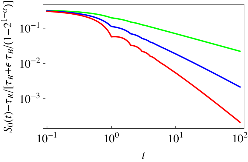
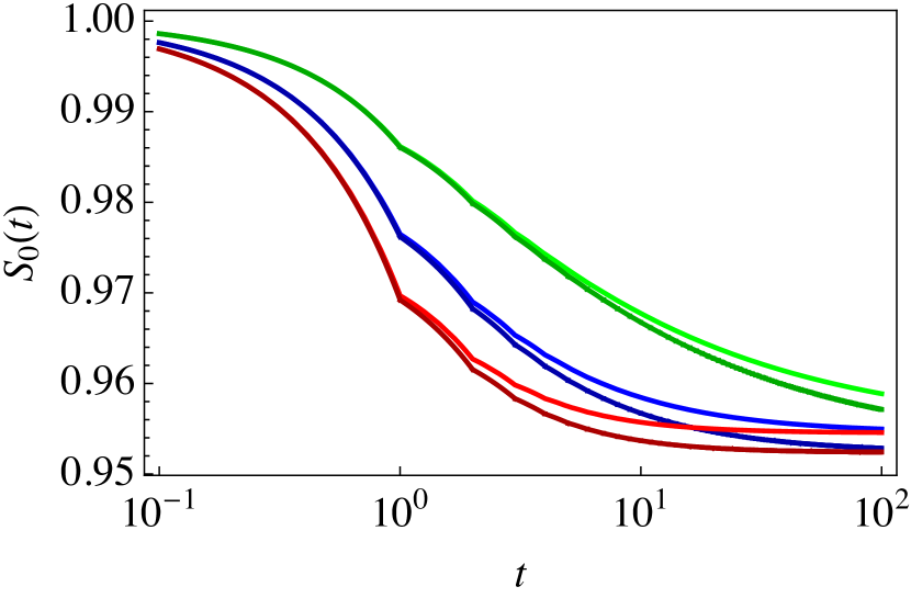
3.2 Small-parameter expansion
Suppose that the scattering parameter is small, , so that the overwhelming majority of transitions occur between scattering states, and only rarely does a particle make an excursion into a propagating state, which may, however, last long, depending on the value of the scaling parameter .
The first-order expansion of equation (26) yields the following approximation of :
| (28) |
That is to say, for , is a sequence of straight line segments joining the values the function takes at integer multiples of the propagation time ,
| (29) |
In this regime, converges asymptotically to the constant value (20), which, for the choice of parameters (7), is given by equation (21), i.e., with all other parameters being fixed,
| (30) |
| (31) |
or, for general time values,
| (32) | ||||
| (33) | ||||
| (34) |
4 Mean squared displacement
Assuming initial injection of particles at the origin, the mean squared displacement of particles as a function of time, given by the second moment of the displacement vector , , where and , evolves according to the differential equation
| (35) |
where, in contrast to the expression derived in reference [16], we have here added possible contributions from source terms , , which we assume to be concentrated at site only. To conform with stationarity of the process, propagating states should be uniformly injected in the time interval so they decay uniformly in the time interval . We thus let ()
| (36) |
where is a sequence of positive numbers such that and is the Heaviside step function, such that the product guarantees the uniform distribution of propagating source terms in the desired time interval. Equation (35) transforms to
| (37) |
Integrating over time, we obtain the mean squared displacement:
| (38) |
There are two contributions to this expression; the first arises from the fraction of particles in a scattering state, and the second from particles initially distributed among propagating states. This term transforms to
| (39) | ||||
| (40) |
4.1 Stationary regimes
The stationary initial condition, i.e. such that the initial fractions of particles in scattering and propagating states are stationary solutions of equations (14)-(17), are realized if, in equation (36), we identify with the stationary fraction of particles in state ,
| (41) |
cf. equation (23), and let
| (42) |
With this choice, the mean squared displacement (38) yields the exact expression
| (43) | ||||
| (44) |
Treating as an integer and letting denote the generalized harmonic numbers, the two terms with sums over in the above expression evaluate respectively to
| (45) |
for the term arising from the fraction of particles in a scattering state, and to
| (46) |
for the term arising from particles initially distributed among the propagating states. Depending on the value of the scaling parameter , we have the following three asymptotic regimes.
4.1.1 Normal diffusion
For parameter values , the asymptotic properties of the harmonic numbers,
| (47) |
are such that only the terms arising from the fraction of particles in a scattering asymptotically contribute to equation (44):
| (48) |
which, up to a factor , is the diffusion coefficient of the process.
4.1.2 Weak superdiffusion
For the marginal parameter value , the harmonic numbers in equation (45) evaluate to
| (49) |
where is Euler’s constant.
We therefore have the asymptotic limit of equation (44),
| (50) |
which is due to the fraction of particles in a scattering state alone. This result is, however, of limited use because the asymptotic regime only emerges provided (where corresponds to the order of the sub-leading term), which may not be attainable, especially when the scattering parameter is small. For this reason, it is preferable to retain also the next-order term in equation (44),
| (51) |
where a fraction is contributed by particles initially distributed among propagating states.
4.1.3 Superdiffusion
In the range of parameters , we substitute the scaling properties of the harmonic numbers,
| (52) |
and obtain from equation (44) the limit
| (53) | ||||
| (54) |
As emphasized by the first line of this equation, the leading-order coefficient is the sum of two distinct non-trivial contributions from the two terms on the right-hand side of equation (44): one from the fraction of particles in a scattering state and the other from particles initially injected in propagating states. As a consequence, the transport coefficient corresponding to the all-scattering initial condition differs by a factor from that above, corresponding to the stationary initial condition. This observation is consistent with the results of reference [25], where non-recurrent regimes of the scaling parameter were also investigated.
4.2 Exact time-dependent solution
The following exact expression of the mean squared displacement (38) is obtained after substitution of the fraction of particles in a scattering state, equation (26), and applies to the all-scattering initial condition (25):
| (55) |
where, for consistency, one must interpret terms such as as unity, even when .
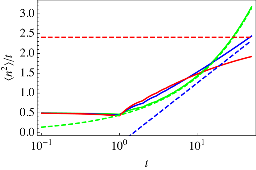
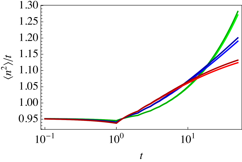
Figure 2 displays the results of explicit evaluations of equation (55) for three different values of the scaling parameter, , with . According to the asymptotic results (48), (50) and (54), the scaling parameter value gives rise to a logarithmic divergence of , which separates the superdiffusive regime, for , from that of normal diffusion, for . A comparison between the exact solution and the asymptotic ones is displayed in figure 2(a). On the time scale of the figure, convergence to the asymptotic regimes is convincingly observed only in the superdiffusive case. Note that while the computation of equation (55) up to takes less than one half hour of CPU time on a reasonably fast computer, doubling the time range would increase the required CPU time to over ten days.
Although equation (55) gives the exact time-dependence of the mean squared displacement of the process for the initial condition (24), it does not give much insight into its time development. In particular, how to extract the large-time behaviour of the mean squared displacement and connect this result to the asymptotic scalings (48), (50) and (54) is not transparent. As reflected by figure 2(a), a numerical evaluation of equation (55) is necessarily limited to moderately large times, due to the number of terms involved.
A regime of specific interest which allows us to infer the emergence of the asymptotic scalings (48), (50) and (54) from the solution (55) is, however, that of small values of the scattering parameter , i.e., such that transitions from scattering to propagating states occur only rarely. This is discussed below. We will otherwise have to resort to numerical simulations of the underlying stochastic processes to observe this convergence. Those results are presented in section 5.
4.3 Small-parameter expansion
For small values of the scattering parameter , when transitions from scattering to propagating states are much rarer than transitions between scattering states, an expansion of equation (55) in powers of this parameter provides an approximate expression of the mean squared displacement from which the different asymptotic regimes discussed in section 4.1 can be inferred. In the anomalous regime of the scaling parameter, , terms constant in time, that carry a normal contribution to the mean squared displacement, may bring about contributions which, even for large times, may be much larger than that of terms diverging in time; an anomalous contribution to the mean squared displacement may then be masked by a normal one.
To proceed, we substitute equation (31) into equation (38) and let . Having dropped all terms of order and higher, we obtain
| (56) | ||||
| (57) | ||||
| (58) | ||||
| (59) | ||||
| (60) | ||||
| (61) |
where, in the last line, we have omitted terms that decay to zero as grows large. Plugging into this expression the asymptotic forms of the generalized harmonic numbers (47), (49) and (52),
| (62) |
we obtain approximations of the mean squared displacement (55), which can be compared with the asymptotic expressions (48), (50) and (54).
In the regime of normal diffusion, , equation (61) reduces to the first order expansion in of equation (48). For , the mean squared displacement (61) displays normal diffusion at short times and anomalous diffusion at large times. Thus in the weak superdiffusive regime, , equation (61) reduces to
| (63) |
which differs from the stationary expression (51) by a factor , subleading with respect to the logarithmically diverging term, identical in both expression. This difference stems from the absence of particles populating propagating states in our choice of initial condition. In the superdiffusive regime, , the divergence of the harmonic numbers, equation (62), dominates the large time behaviour,
| (64) |
Here again we note a difference between this expression and equation (54), obtained in the stationary regime. At variance with the case , however, the difference occurs in the coefficient of the leading term on the right-hand side of equation (64), whose numerator is instead of in the stationary regime. The transport coefficient on the right-hand side of equation (64) therefore changes, depending on the choice of initial conditions.
At large times, after the mean squared displacement crosses over from normal diffusion to superdiffusion, the above expressions are equivalent to expansions of the asymptotic values (50) and (54). The value of the crossover time, , that separates the short time normal diffusion from the large time anomalous diffusion can be inferred from the above expressions:
| (65) |
which can be large, in particular when .
For short times, equation (61) can be improved by removing the assumption that is an integer multiple of . One then finds
| (66) | ||||
| (67) | ||||
| (68) | ||||
| (69) | ||||
| (70) | ||||
| (71) | ||||
| (72) |
5 Numerical computations
Numerical simulations of the process with rates (2) and probabilities (3) are based on a classic kinetic Monte Carlo algorithm [26], taking into account the possibility of ballistic motion of particles in a propagating phase.
A collection of independent walkers are initialized at time at the origin of the two-dimensional square lattice , either in the scattering state, , for the all-scattering initial condition, or in state with relative weights specified by equations (41)–(42), for the stationary initial condition. For each walker, we generate a sequence of successive states , , , and corresponding times as follows.
When in a state , the next transition is determined by drawing the following three random numbers. This is referred to as a scattering step.
-
(i)
The first random number, , is drawn from a uniform distribution, and yields the state , such that .
-
(ii)
The corresponding waiting time, i.e., the time the particle waits in the state before the transition to state takes place, is obtained by drawing a second random number, whose distribution is exponential with mean .
-
(iii)
A third random integer, with uniform distribution among the set of lattice directions , identifies the direction of the corresponding displacement by one lattice unit.
Depending on the new state , another scattering step is taken if or, if , a sequence of propagating steps takes place, such that:
-
(i)
the state decreases by one unit, ,
-
(ii)
the direction remains unchanged , and
-
(iii)
the time step takes value , corresponding to the propagation time over a single lattice cell.
The above loop repeats itself until , that is until , at which point another scattering step is taken.
Keeping track of the positions of all walkers as functions of time, which we measure at regular intervals on a logarithmic timescale, measurements of the mean squared displacement rescaled by are performed by taking averages of this quantity over the set of all walkers, which typically consists of trajectories. Such measurements are reported below for the different scaling regimes in the positive recurrent range of the scaling parameter values, .
Throughout this section, we set the transition probabilities according to equation (7) and, for convenience, change the scattering parameter to
| (73) |
We further let
| (74) |
such that the asymptotic fraction of particles in the scattering state (21) becomes
| (75) |
5.1 All-scattering vs. stationary initial conditions
With the choice of parameters (73)-(74), The mean squared displacement, for large and with the all-scattering initial condition, is expected to scale as
| (76) |
where, in the two anomalous cases, we kept terms constant in time to reflect the possibility that, when is small, the normal term may not be negligible with respect to the anomalous one over a large range of times. This is particularly relevant for the marginal case, , where and remain of comparable sizes throughout the time range accessible to numerical computations. In comparison, for the stationary initial condition, the above expression remains unchanged in the normal diffusive case, but is modified in the two anomalous cases,
| (77) |
The first order expansion in of the two anomalous regimes in equation (76) (in all-scattering initial condition) yields results equivalent to equations (63) and (64) respectively.
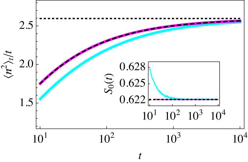
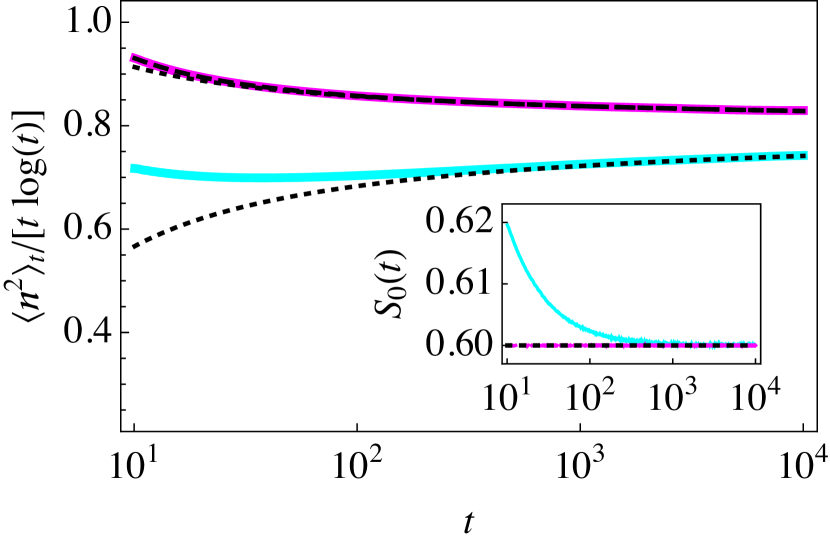
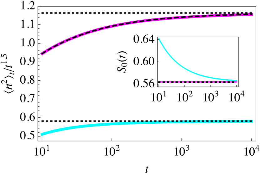
A computation of the time evolution of the mean squared displacement in regimes of normal () and anomalous () diffusion is shown in figure 3, providing a comparison between the two initial conditions analyzed in section 4, with the two corresponding sets of asymptotic regimes given by equations (76) and (77). The scaling parameter values are set to (figure 3(a)), (figure 3(b)), and (figure 3(c)). The scattering parameter value is set to throughout, such that transitions between scattering states are forbidden. As expected, the numerically computed mean squared displacement obtained from the stationary initial condition (magenta curves in figures 3(a)-3(c)) follow precisely the analytic result (44) in all three regimes.
We further note that, in the regime of normal diffusion (), both data sets in figure 3(a) display consistent convergence to the same asymptotic regime, given by the first lines of equations (76) and (77), . A similar result is observed in figure 3(b), where the convergence of the two data sets to the common leading value of equations (76) and (77), , is apparent. The effect of the differing subleading terms, the one in (76) negative, the other in (77) positive (the latter value is about one half the absolute value of the former for ), is, however, manifest. Finally, in the superdiffusive regime, , figure 3(c) exhibits the two asymptotic regimes of the anomalously rescaled mean squared displacement given by equations (76) and (77), (all-scattering initial condition) or (stationary initial condition), whose values differ by a ratio for this value of the scaling parameter.
5.2 Perturbative regimes of the scattering parameter
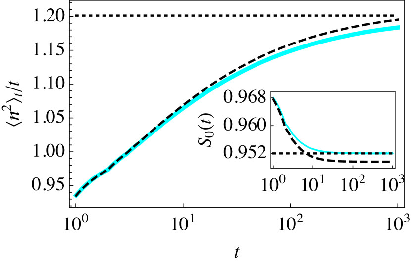
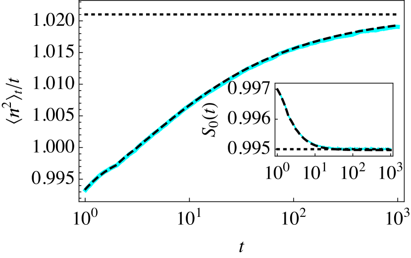
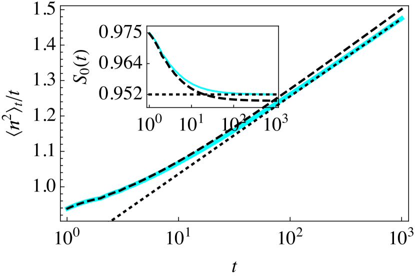
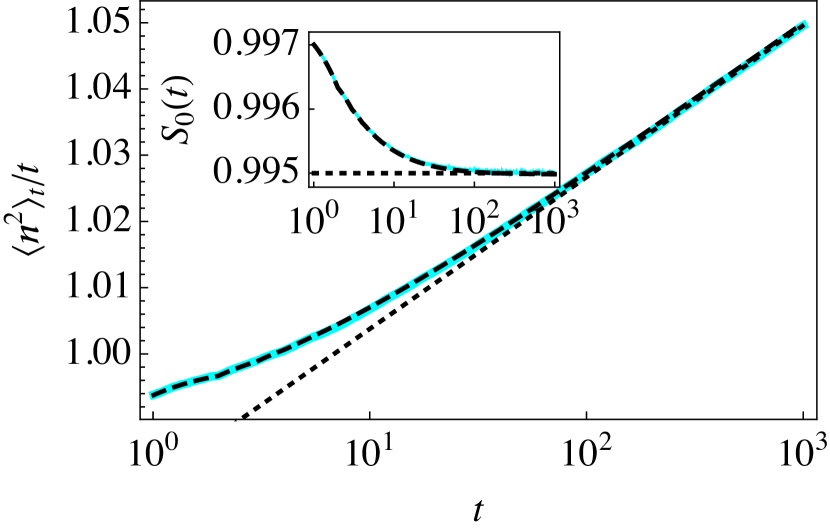
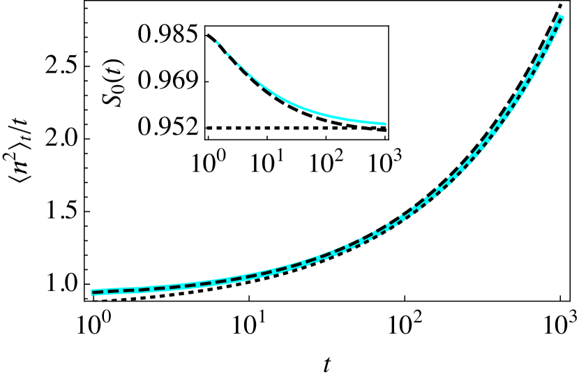
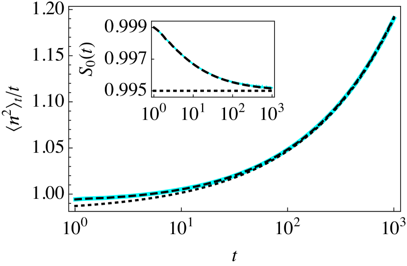
The time evolution of the mean squared displacement in the perturbative regime of the scattering parameter, , is analyzed in figure 4 for particles initially distributed in the scattering state at the origin, where the rescaled mean squared displacement is compared with the solution, equation (72). Excellent agreement between the analytic and numerical results is observed throughout the time range when the parameter is small enough ( figures 4(b), 4(d), 4(f)). Numerical computations are also consistent with the asymptotic regime (76) for all cases.
The scattering parameter value , shown in figures 4(a) (), 4(c) (), and 4(e) (), is on the one hand small enough that, for short times, the computed mean squared displacement is barely distinguishable from the perturbative expansion (72). The effect of next order corrections is, on the other hand, apparent for larger times (), beyond which a convergence to the asymptotic result (76) is observed.
We note that the crossover time (65) is for (figure 4(c)) and much larger yet for . For , subleading terms in equation (76) therefore dominate the logarithmically divergent term throughout the time range of measurements. Similarly, in the superdiffusive case, , the respective crossover times (65) are (figure 4(e)) and (figure 4(f)), such that subleading terms in equation (76) remain important throughout the time range of measurements in both cases.
We conclude this section by pointing out that the time range of numerical measurements such as presented in figure 4 is limited by the finite precision of the random number generator used to draw the transition probabilities and sets an effective maximal scale of free flights, . This observation is analogous to the effect of machine-dependent limitations recently reported in reference [27] and is particularly relevant to the regime of weak superdiffusion. The effective maximal scale induces a saturation of the logarithmic growth of the second moment for times larger than . The process would thus become diffusive for times sufficiently large. Although this effect can be pushed upward to larger times by increasing the precision of the random number generator, it cannot be eliminated altogether.
6 Conclusions
The inclusion of exponentially-distributed waiting times separating the successive jump events of Lévy walkers leads to a natural distinction between propagating and scattering states, whose respective concentrations evolve in time according to a set of generalized master equations. In particular, the fraction of walkers in a scattering state obeys a linear delay differential equation with a countable hierarchy of delays whose analytic solutions were obtained.
As opposed to classic methods based on the Fourier–Laplace transform of an integral kernel and the use of Tauberian theorems [11, 13], the approach presented in this paper is based solely on the solutions of such delay differential equations. Our method thus yields a simple expression of the mean squared displacement of Lévy walkers in terms of the distribution of free paths and the time integral of the fraction of particles in the scattering state.
Both exact and asymptotic expressions of the mean squared displacement of walkers were obtained in regimes ranging from normal to superdiffusive subballistic transport. In these regimes, the mechanism through which a walker can change directions between successive propagation phases plays an important role in determining the values of the transport coefficients, whether normal or anomalous. The transition through a scattering phase brings about a description in terms of two parameters, the first specifying the typical timescale of scattering events as opposed to the timescale of propagation across an elementary cell, the second weighting the probability of transitions between scattering and propagating states.
Relying on the stationary fractions of particles in scattering and propagating states, a detailed derivation of the transport coefficients, similar to that reported in [16], was given, exhibiting the precise effect of the two scattering parameters on these coefficients, as well as the influence of the initial distribution of walkers [25]. Our formalism also yields the exact time evolution of the mean squared displacement, which was investigated when particles are initially found in a scattering state.
The comparison between the exact and asymptotic solutions is generally not immediate, but is fairly straightforward in perturbative regimes such that the likelihood of a transition from scattering to propagating states is small. A case in point – though by far not the only application of the present results – is given by the infinite-horizon Lorentz gas [28], for which the scaling parameter of the distribution of free paths takes on the marginal value . As one might expect, measuring the logarithmic divergence in time of the rescaled mean squared displacement is typically hindered by dominant constant terms. This is particularly so in the regime of narrow corridors, which yields a stochastic description in terms of multistate Lévy walks such that the scattering parameter is small, [23]. The parameter induces a further separation between the time scales of the scattering and propagating phases, . To accurately model the scattering phase is therefore of paramount importance to understanding the dynamics of the infinite-horizon Lorentz gas in terms of a Lévy walk.
The results obtained in this paper provide the framework to transposing such results to a range of applications exhibiting other regimes of transport, such as have been studied in the context of optimal intermittent search strategies [22]. Our theoretical framework brings about new perspectives to extend the study of intermittent walks to power-law distributed ballistic phases, which may be relevant to the increasing body of literature on optimal search strategies [8, 29, 30].
Appendix A Time-dependent fraction of particles in the scattering state
To derive equation (26), we note that and, for ,
| (78) |
By recursive application of this formula, we obtain
| (79) |
which is equivalent to equation (27).
| (80) |
We have to show that the last term on the RHS vanishes, which amounts to proving the identity
| (81) |
or, after rearrangement,
| (82) |
The second term in this expression, by successively changing the index to , then swapping the sums over and and exchanging the indices and , transforms to
| (83) |
Now swapping the sums over and in the last line and plugging this expression back into equation (82), we obtain, after factorization of the common factors, the condition
| (84) |
References
References
- [1] Shlesinger M F, Zaslavsky G M and Frisch U (eds) 1995 Lévy Flights and Related Topics in Physics (Lecture Notes in Physics vol 450) (Berlin Heidelberg: Springer) URL http://dx.doi.org/10.1007/3-540-59222-9
- [2] Klafter J, Shlesinger M F and Zumofen G 1996 Physics Today 49 33–39 URL http://dx.doi.org/10.1063/1.881487
- [3] Klages R, Radons G and Sokolov I M 2008 Anomalous transport: Foundations and applications (Weinheim: Wiley-VCH Verlag) URL http://dx.doi.org/10.1002/9783527622979
- [4] Denisov S, Zaburdaev V Y and Hänggi P 2012 Physical Review E 85 31148 URL http://dx.doi.org/10.1103/PhysRevE.85.031148
- [5] Zaburdaev V, Denisov S and Klafter J 2014 arXiv:1410.5100 URL http://arxiv.org/abs/1410.5100
- [6] Weiss G H and Rubin R J 1983 Advances in Chemical Physics 52 363–505 URL http://dx.doi.org/10.1002/9780470142769.ch5
- [7] Shlesinger M F, Zaslavsky G M and Klafter J 1993 Nature 363 31–37 URL http://dx.doi.org/10.1038/363031a0
- [8] Viswanathan G M, da Luz M G E, Raposo E P and Stanley H E 2011 The Physics of Foraging: an Introduction to Random Searches and Biological Encounters (Cambridge, UK: Cambridge University Press) URL http://www.cambridge.org/9781107006799
- [9] Brockmann D, Hufnagel L and Geisel T 2006 Nature 439 462–465 URL http://dx.doi.org/10.1038/nature04292
- [10] Raichlen D A, Wood B M, Gordon A D, Mabulla A Z, Marlowe F W and Pontzer H 2014 Proceedings of the National Academy of Sciences of the United States of America 111 728–733 URL http://dx.doi.org/10.1073/pnas.1318616111
- [11] Geisel T, Nierwetberg J and Zacherl A 1985 Physical Review Letters 54(7) 616–619 URL http://dx.doi.org/10.1103/PhysRevLett.54.616
- [12] Shlesinger M F and Klafter J 1985 Physical Review Letters 54 2551–2551 URL http://dx.doi.org/10.1103/PhysRevLett.54.2551
- [13] Klafter J, Blumen A and Shlesinger M F 1987 Physical Review A 35 3081–3085 URL http://dx.doi.org/10.1103/PhysRevA.35.3081
- [14] Wang X J 1992 Physical Review A 45(12) 8407–8417 URL http://dx.doi.org/10.1103/PhysRevA.45.8407
- [15] Zumofen G and Klafter J 1993 Physical Review E 47(2) 851–863 URL http://dx.doi.org/10.1103/PhysRevE.47.851
- [16] Cristadoro G, Gilbert T, Lenci M and Sanders D P 2014 EPL (Europhysics Letters) 108 50002 URL http://dx.doi.org/10.1209/0295-5075/108/50002
- [17] Landman U, Montroll E W and Shlesinger M F 1977 Proceedings of the National Academy of Sciences of the United States of America 74 430–433 URL http://www.pnas.org/content/74/2/430.abstract
- [18] Montroll E W and Weiss G H 1965 Journal of Mathematical Physics 6 167 URL http://dx.doi.org/10.1063/1.1704269
- [19] Kenkre V M, Montroll E W and Shlesinger M F 1973 Journal of Statistical Physics 9 45–50 URL http://dx.doi.org/10.1007/BF01016796
- [20] Klafter J, Zumofen G and Shlesinger M F 1995 Lévy description of anomalous diffusion in dynamical systems Lévy Flights and Related Topics in Physics (Lecture Notes in Physics vol 450) ed Shlesinger M F, Zaslavsky G M and Frisch U (Berlin Heidelberg: Springer) pp 196–215 URL http://dx.doi.org/10.1007/3-540-59222-9_35
- [21] Klafter J and Sokolov I M 2011 First steps in random walks: from tools to applications (Oxford, UK: Oxford University Press) ISBN 9780199234868 URL http://dx.doi.org/10.1093/acprof:oso/9780199234868.001.0001
- [22] Bénichou O, Loverdo C, Moreau M and Voituriez R 2011 Reviews of Modern Physics 83 81 URL http://dx.doi.org/10.1103/RevModPhys.83.81
- [23] Cristadoro G, Gilbert T, Lenci M and Sanders D P 2014 Physical Review E 90(5) 050102 URL http://dx.doi.org/10.1103/PhysRevE.90.050102
- [24] Driver R D 1977 Ordinary and delay differential equations (New York, NY: Springer-Verlag) URL http://dx.doi.org/10.1007/978-1-4684-9467-9
- [25] Zumofen G and Klafter J 1993 Physica D 69 436–446 URL http://dx.doi.org/10.1016/0167-2789(93)90105-A
- [26] Gillespie D T 1976 Journal of Computational Physics 22 403–434 URL http://dx.doi.org/10.1016/0021-9991(76)90041-3
- [27] Radicchi F 2014 Physical Review E 90(5) 050801 URL http://dx.doi.org/10.1103/PhysRevE.90.050801
- [28] Cristadoro G, Gilbert T, Lenci M and Sanders D P 2014 Physical Review E 90(2) 022106 URL http://dx.doi.org/10.1103/PhysRevE.90.022106
- [29] Lewis M A, Maini P K and Petrovskii S V (eds) 2013 Dispersal, individual movement and spatial ecology (Lecture Notes in Mathematics vol 2071) (Berlin: Springer) URL http://dx.doi.org/10.1007/978-3-642-35497-7
- [30] Méndez V, Campos D and Bartumeus F 2013 Stochastic Foundations in Movement Ecology (Berlin, Heidelberg: Springer) URL http://dx.doi.org/10.1007/978-3-642-39010-4