Theory of fads: Traveling-wave solution of evolutionary dynamics in a one-dimensional trait space

Abstract

We consider an infinite-sized population where an infinite number of traits compete simultaneously. The replicator equation with a diffusive term describes time evolution of the probability distribution over the traits due to selection and mutation on a mean-field level. We argue that this dynamics can be expressed as a variant of the Fisher equation with high-order correction terms. The equation has a traveling-wave solution, and the phase-space method shows how the wave shape depends on the correction. We compare this solution with empirical time-series data of given names in Quebec, treating it as a descriptive model for the observed patterns. Our model explains the reason that many names exhibit a similar pattern of the rise and fall as time goes by. At the same time, we have found that their dissimilarities are also statistically significant.

I Introduction

Sir Isaac Newton reportedly said that he could calculate the motion of heavenly bodies but not the madness of people, when he had lost a fortune in the South Sea Bubble. Since his time, there have been vigorous attempts to apply the so-called Newtonian approach to our society in order to understand the ‘madness of people’. It is interesting that some of modern economists have finally explained bubbles as based on rational expectation Camerer (1989); Schaller and van Norden (2002), although it does not mean that bubbles are really under our control. At the same time, they distinguish a fad from a bubble as the former originates solely from social forces, which are harder to rationalize from an economic point of view. Even if we take a more phenomenological viewpoint, how this social influence organizes itself seems to remain largely unpredictable. A society adopts some practices and abandons some others constantly, but it is neither a matter of practical use nor that of aesthetic superiority. One might say that it is because something is ‘cool’, but it hardly explains anything but the unpredictability. It is another, perhaps a worse kind of ‘madness’ from a physicist’s point of view.

Given names are subject to fads Zanette ; Kessler et al. (2012). It is sharply contrasted to the case of family names, whose dynamics is well defined by mathematical models Zanette and Manrubia (2001); Reed and Hughes (2003); Baek et al. (2007); Rossi (2013). If a certain given name prevails, on the other hand, it is simply because it sounds cool, i.e., for no particular reason. Note that being a fad in this context does not necessarily mean that it is short-lived: For example, Michael was the most popular name in the United States for about half a century from the 1950s com . Our point is that such popularity is not explained by any of its intrinsic properties, and we will call it a fad regardless of the time scale. Even if it is difficult to predict a fad, e.g., what will be the most popular name for babies next year, one may still expect a higher degree of regularity in the rise and fall of each given name. Fortunately, there is an available data set, compiled by Duchesne, which has recorded frequencies of $100$ major given names in the Canadian province of Quebec for more than a century Duchesne (2001); sta . It is basically a collection of names given to a certain number of people each year, from which the fractions of the given names are calculated. This collection is also called a corpus and its size, i.e., the number of people surveyed, has been greater than $2\times 10^{3}$ every year throughout the 20th century. In Fig. 1, the shade represents the fraction, and the names are sorted according to the mean time of prevalence, defined as

$$\left<t\right>=\frac{\sum_{t}tf(t)}{\sum_{t}f(t)},$$ (1)

where $t$ runs from year 1900 to 2000, and $f(t)$ is the fraction of a particular name in year $t$. This plot suggests the existence of a certain regular pattern. That is, fads propagate with forming a traveling wave across the space of names, from one name to another, and it is more clearly seen for female names. In addition, the narrower width of the name distribution along the vertical axis in Fig. 1(b) indicates that the change is more rapid for girls’ names. This observation implies that the female-name dynamics is probably simpler, in the sense that one only has to be concerned about how his or her daughter’s name will sound to others. Based on this observation, we will construct a descriptive model for the pattern in the female names. While the existing models in Refs. Zanette, ; Kessler et al., 2012 consider the dynamics of a single name interacting with the environment, we are more interested in describing the competition among many names that takes place simultaneously. This many-body problem reduces to a reaction-diffusion system written in terms of the frequency distribution of newborn children’s given names, yielding a traveling-wave solution. By comparing the model with the empirical data, we will check whether our picture captures essential parts of the dynamics.

Figure 1: (a) Fractions of a hundred male given names and (b) those of the same number of female given names in Quebec, from year $1900$ to $2000$. The names are sorted in an ascending order of the mean time of prevalence [Eq. (1)].

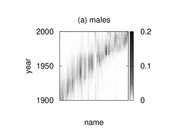
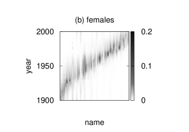
This work is organized as follows. The next section presents our model, formulated as a generalized version of the Fisher equation Fisher (1937). Section III then explains how we analyze the empirical data and compare them with our model. In this section, the goodness of fit will be quantitatively estimated with a statistical test. After discussing the result in Sec. IV, we conclude this work.

II Model

Our starting point is adoption-exploration dynamics of idea spreading Baek et al. (2013). According to this theory, we may imagine that each given name behaves as a biological species, competing to win as many adopters as possible. In other words, given names are assumed to obey certain evolutionary dynamics. To formulate this dynamics in mathematical terms, we need a number (or a set of numbers) to quantify the competitiveness of each name relative to that of others. Just as a species is said to have its own fitness Kimbrough (1980); Orr (2009), therefore, let us furthermore assume that it is possible to assign a certain value of ‘fitness’, represented by a real number $x$, to each given name. Our viewpoint is that the names are arranged and indexed by this fitness measure, and a name with $x$ is picked up by a newborn baby’s parents from a certain probability distribution function. Note that our formulation mainly concerns how likely a name will be chosen for a newborn baby, rather than the fraction of all the people carrying that name. It is also important to remember that each given name has a fixed value of $x$, which is independent of time $t$, so that we can effectively map each $x$ to a different name. For this reason, one can think of $x$ as a position in the space of names, analogous to the horizontal axis in Fig. 1, although we do not actually have to determine the values for the data set in our analysis as will be seen below. So it is the fraction of $x$, instead of its value, that changes with time. Due to the growth of the fitter, the distribution will move to higher values of $x$ in general. As a result, a time series for a specific given name can be unimodal at best. This might not be strictly true in Western countries Kessler et al. (2012). But in Quebec, only a few percent of names succeed to come back. In our data set, therefore, such recurrence as considered in Ref. Kessler et al., 2012 can rather be treated as exceptional.

Let us consider the following adoption-exploration dynamics Baek et al. (2013):

$$\frac{\partial P}{\partial t}=k(U-\left<U\right>)P+D\frac{\partial^{2}P}{\partial x^{2}},$$ (2)

where $P=P(x,t)$ is the probability density function at time $t$ for finding a ‘species’ of fitness $x\in(-\infty,+\infty)$, $U=U(x,t)$ is the payoff that the species gains, and $\left<U\right>$ is the population average of $U(x,t)$ defined as $\left<U\right>\equiv\int dxU(x,t)P(x,t)$. The first term on the right-hand side (RHS) means that $P(x,t)$ has a relative growth rate proportional to $U(x,t)$, in a similar spirit to the replicator equation in evolutionary biology Taylor and Jonker (1978); Hofbauer et al. (1979); Maynard Smith (1982). One may also refer to Ref. Oechssler and Riedel, 2001 for mathematical aspects of a replicator equation on a continuous trait space. The second term on the RHS describes exploratory activities for new traits as diffusion along the $x$ axis. The positive parameters $k$ and $D$ are thus called the rate of adoption and a measure of exploration, respectively. It is instructive to compare this with Eigen’s phenomenological theory of selection Eigen (1971); Ebeling et al. (1984). From our perspective, it is important that this theory of selection can generally be applied to any information carriers that reproduce themselves, including memes. The theory starts with the following rate equation for $P_{i}$, the concentration of an information carrier $i$ ($i=1,\ldots,n$):

$$\frac{d}{dt}P_{i}=F_{i}P_{i}-R_{i}P_{i}+\sum_{j}(\phi_{ij}P_{j}-\phi_{ji}P_{i}),$$ (3)

where the first and second terms refer to self-instructed reproduction and removal of the carrier, respectively, whereas the last summation contains all the other production such as mutation. As one of possible conditions for selection, we may choose $\sum_{i}P_{i}=\mbox{const}$. The reproduction and removal can be specified further as follows: Let us set $F_{i}=k_{0}A_{i}Q_{i}$, where $k_{0}$ is a rate constant, $A_{i}$ is an amplification factor, and $Q_{i}$ is a quality factor of precise reproduction. Likewise, we set $R_{i}=k_{0}B_{i}+\phi_{0}$, where $B_{i}$ is a decomposition factor and $\phi_{0}$ is a dilution factor, which is controlled by the boundary condition and assumed to be independent of $i$. We now obtain a more detailed form of the rate equation:

$$\frac{d}{dt}P_{i}=k_{0}\left(A_{i}Q_{i}-B_{i}\right)P_{i}+\sum_{j}(\phi_{ij}P_{j}-\phi_{ji}P_{i})-\phi_{0}P_{i}.$$ (4)

If we sum up both sides of Eq. (4) over $i$, we find that

$$0=\sum_{i}k_{0}\left(A_{i}Q_{i}-B_{i}\right)P_{i}-\phi_{0}\sum_{i}P_{i},$$ (5)

because $\sum_{i}\sum_{j}(\phi_{ij}P_{j}-\phi_{ji}P_{i})$ identically vanishes. If we define a selective value as $U_{i}=A_{i}Q_{i}-B_{i}$, Eq. (5) means that $\phi_{0}=k_{0}\sum_{i}U_{i}P_{i}/\sum_{i}P_{i}=k_{0}\left<U\right>$. Equation (4) is thus rewritten as

$$\frac{d}{dt}P_{i}=k_{0}\left(U_{i}-\left<U\right>\right)P_{i}+\sum_{j}(\phi_{ij}P_{j}-\phi_{ji}P_{i}).$$ (6)

Supposing that the mutation rates $\phi_{ij}$ are symmetric, homogeneous, and short-ranged in the index space, one can approximate the last term by a second-order differential and derive Eq. (2) through a suitable limiting process Ebeling et al. (1984).

It has been suggested in Ref. Baek et al., 2013 that $U(x,t)$ can be identified with the cumulative distribution $C(x,t)\equiv\int_{-\infty}^{x}P(x^{\prime},t)dx^{\prime}$ up to a proportionality coefficient absorbed into $k$, because those with $x^{\prime}<x$ are potential adopters of $x$. In the general context of fads, however, the payoff function might not be such a simple linear function of $C(x,t)$. For example, there can be an adverse effect of being too popular. Let us generalize the above argument in the following way: We assume that there eventually develops a traveling wave with speed $v$ and a unimodal shape of $P(x-vt)$. At any time, the corresponding $C(x)$ should be a monotonically increasing smooth function of $x$ within a certain region. Our claim is that it can then be used as a basis for expressing an arbitrary shape of $U(x)$ within the region of our interest. The idea is as follows: If we define $\mu\equiv C(x)$, there is one-to-one correspondence between $x$ and $\mu$ as long as $P>0$, and one can write $U$ as a function of $\mu$ instead of $x$. We expand $U(\mu)$ as a polynomial in $\mu$, i.e., $U=a_{0}+a_{1}\mu+a_{2}\mu^{2}+\cdots=a_{0}+a_{1}C(x)+a_{2}C^{2}(x)+\cdots$ with coefficients $a_{i}$. Clearly, $a_{0}$ does not alter the dynamics as $\left<U\right>$ is subtracted, and $a_{1}$ is absorbed into the equation by rescaling the time scale. We will therefore retain the two lowest-order contributions as $U(x,t)=C(x,t)+\frac{3}{2}gC^{2}(x,t)$ with a constant $g$, where the factor of $\frac{3}{2}$ is added for later convenience. This constant $g$ is introduced as a shape parameter to control the skewness of the distribution, but it can also be interpreted as the population’s preference to new fads. If $g$ is negative, for example, it means that the population is ‘conservative’ in the sense that the fitness $U$ does not increase with $x$ as sharply as it would under positive $g$. Noting that

$$\int_{-\infty}^{\infty}C^{n}Pdx=\int_{0}^{1}C^{n}dC=\frac{1}{n+1},$$ (7)

we rewrite Eq. (2) as

$$\frac{\partial P}{\partial t}=k\left[C+\frac{3}{2}gC^{2}-\frac{1}{2}(1+g)\right]P+D\frac{\partial^{2}P}{\partial x^{2}}.$$ (8)

By rescaling $t$ and $x$ as $kt$ and $x\sqrt{k/D}$, respectively, we reduce the equation to

$$\frac{\partial P}{\partial t}=\left[C+\frac{3}{2}gC^{2}-\frac{1}{2}(1+g)\right]P+\frac{\partial^{2}P}{\partial x^{2}}.$$ (9)

By using $\frac{\partial C}{\partial x}=P$, this can be written as

$$\frac{\partial^{2}C}{\partial t\partial x}=\frac{\partial}{\partial x}\left[\frac{C^{2}}{2}+\frac{g}{2}C^{3}-\frac{1}{2}(1+g)C+\frac{\partial^{2}C}{\partial x^{2}}\right],$$ (10)

which implies that

$$\frac{\partial C}{\partial t}=\frac{1}{2}C(C-1)(gC+g+1)+\frac{\partial^{2}C}{\partial x^{2}}+\sigma(t),$$ (11)

where $\sigma(t)$ is a function of $t$ only. Substituting $x=\pm\infty$, we find that $\sigma(t)=0$ because the left-hand side and the first two terms in the RHS identically vanish there. To sum up, we will consider the following equation:

$$\frac{\partial C}{\partial t}=\frac{1}{2}C(C-1)(gC+g+1)+\frac{\partial^{2}C}{\partial x^{2}}.$$ (12)

This form is close to the Zeldovich equation Zeldovich and Frank-Kamenetsky (1938), although the phase-space structure is different as will be detailed below. If $g=0$, this is mathematically equivalent to the celebrated Fisher equation Fisher (1937). This model can also be interpreted in terms of the activator-inhibitor model in Ref. Zanette, (see Appendix A for details). In addition, one may recall that a spin system is phenomenologically expressed by the time-dependent Ginzburg-Landau equation as

$$\frac{\partial m}{\partial t}=m-m^{3}+\nabla^{2}m,$$ (13)

where $m$ denotes the order parameter Krapivsky et al. (2010). One keeps the linear and cubic terms of $m$ to describe the symmetric double-well structure of the free-energy density functional. In this respect, the additional term proportional to $g$ in deriving Eq. (12) can be interpreted as introducing a cubic term to the RHS, although we are not dealing with a magnetic system.

The assumption of the traveling wave implies that $C(x,t)=C\left(x-vt\right)$, where $v$ is the speed. In a moving frame with coordinate $\eta\equiv x-vt$, Eq. (12) describes the shape of the wave as a second-order ordinary differential equation:

$$-v\frac{dC}{d\eta}=\frac{1}{2}C(C-1)(gC+g+1)+\frac{d^{2}C}{d\eta^{2}},$$ (14)

or, equivalently, a set of two first-order ordinary differential equations:

$$\left\{\begin{array}[]{lcl}dC/d\eta&=&P\\ dP/d\eta&=&-vP-\frac{1}{2}C(C-1)(gC+g+1),\end{array}\right.$$ (15)

where the first line relates the probability density function $P$ and its cumulative $C$. This system has three fixed points at $(C,P)=(0,0)$, $(1,0)$, and $(-1-g^{-1},0)$. The linear stability analysis shows that the eigensystem around the origin consists of eigenvalues $\lambda_{\pm}=\frac{1}{2}\left[-v\pm\sqrt{v^{2}+2+2g}\right]$ and eigenvectors

$$\mathbf{y}_{\pm}=\left(\begin{array}[]{c}1\\ \lambda_{\pm}\end{array}\right).$$ (16)

On the other hand, the eigensystem in the vicinity of $(C,P)=(1,0)$ is obtained as $\mu_{\pm}=\frac{1}{2}\left(-v\pm\sqrt{v^{2}-4g-2}\right)$, together with the corresponding eigenvectors:

$$\mathbf{z}_{\pm}=\left(\begin{array}[]{c}1\\ \mu_{\pm}\end{array}\right).$$ (17)

If $v<\sqrt{4g+2}$, the eigenvalues become complex, which is not physically reasonable because $C$ would not be bounded within the unit interval. This proves the existence of the minimum speed $v_{\rm min}=\sqrt{4g+2}$ below which one cannot find a traveling-wave solution (see Appendix B for more discussion and references on the speed selection principle). If $g=-\frac{1}{2}$, the wave can stop, meaning that the population is so conservative that there might be no progression to higher $x$. The last fixed point at $(C,P)=(-1-g^{-1},0)$ has an eigensystem of $\zeta_{\pm}=\frac{1}{2}\left[-v\pm\sqrt{v^{2}-4g^{2}-6-2g^{-1}}\right]$ and

$$\mathbf{w}_{\pm}=\left(\begin{array}[]{c}1\\ \zeta_{\pm}\end{array}\right).$$ (18)

The last fixed point should not lie between the other two, because it is meant to modify the flow from $(0,0)$ to $(1,0)$, leaving the overall phase-space structure unaltered. This restricts the possible range of $g$ to $g\geq-\frac{1}{2}$.

Figure 2: (Color online) $P$ versus $C$, where $P$ is scaled by its maximum amplitude $P_{\rm max}$. The speed is chosen as $v=2$. Note that the flow of Eq. (15) goes from $(C,P)=(0,0)$ to $(1,0)$ as $\eta\equiv x-vt$ increases. (a) The solid line with $g=+0.4$ has $\frac{dP}{dC}>0$ at $C=\frac{1}{2}$ in this plot, and $P(\eta)$ has negative skewness. If we fix $x$ and observe its time series as $t$ varies, therefore, the height grows rapidly and then decreases slowly. (b) The dotted line with $g=-0.4$ shows the opposite case, as explained in the main text.

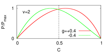
With this parameter $g$, one can control the skewness of the wave shape: Consider a trajectory from $(0,0)$ to $(1,0)$ in the $(C,P)$ plane, as described by Eq. (15). If the shape of $P(\eta)$ is negatively skewed, we will see $\frac{dP}{dC}>0$ at $C=\frac{1}{2}$, and vice versa (Fig. 2). Setting $C=\frac{1}{2}$, we see from Eq. (15) that

$$\frac{dP}{dC}=-v+\frac{1+3g/2}{8P^{\ast}},$$ (19)

where $P^{\ast}$ is the value of $P$ when $C=\frac{1}{2}$. Equation (19) shows that one can change the sign of $\frac{dP}{dC}$, hence the skewness, by modulating $g$. It is not a linear relationship, though, because $P^{\ast}$ also depends on $v$ and $g$. A negative value of $g$ close to its lower bound $-\frac{1}{2}$ will lead to a positively skewed shape of $P(\eta)$ (see Fig. 2). As this wave travels in time, we will see that fads are adopted slowly and then abandoned rapidly, compared with the case of positive $g$.

III Data Analysis

Figure 3: (Color online) (a) More than two-thirds of the names show left-skewed $P(\tilde{\eta})$, and one such example is plotted here. It means that they quickly become popular and then slowly disappear, because $\tilde{\eta}\propto-t$. The noisy curve represents the corpus data, and the smooth one is obtained from our model. This example is fitted with $v=1.7$ and $g=-0.06$ (see the main text for details of the fitting). (b) A dozen of names are equally well or better fitted to right-skewed distribution. The fitting parameters are $v=2.4$ and $g=-0.43$ in this example. (c) Recurrence is observed for a couple of names like Gabrielle and Marie-Anne, roughly with a centennial period. (d) There are a few ‘steady sellers’, including Rachel and Élisabeth, with no particular patterns.

For given $v$ and $g$, we can obtain $P(\eta)=P(x-vt)$ by numerically integrating Eq. (15). It is not directly observable, however, because it is difficult to measure $x$ in practice. The available data set is given as a collection of time series, one for each different given name. If we choose one of them, $x$ is fixed by assumption, and the observed time series corresponds to $P(t-x/v)$. That is, if compared with the hypothetical distribution $P(\eta)$, the time series would be a reflected and scaled image along the horizontal axis. Let us stress the underlying assumptions behind this statement: First, the parameters such as $v$ and $g$ are assumed to be stationary, at least approximately, to relate the observed time series to $P(\eta)$. Second, our model assumes that every name is equal, except for its value $x$. Therefore, in principle, every name is expected to exhibit a similar pattern in its time series. Recall that each time series should be related to others by time translation, because it appears as $P(t-x/v)$. For each time series to be regarded as a projected image of a probability distribution function, therefore, our data should be traced backward with normalizing the area under the curve to one. In other words, the time series $f(t)$ up to $t=t_{\rm max}$ transforms to $f(t_{\rm max}-t)/\sum_{t}f(t)$, which we denote as $P(\tilde{\eta})$ with $\tilde{\eta}\equiv t_{\rm max}-t$.

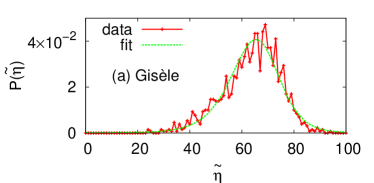
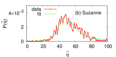
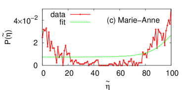
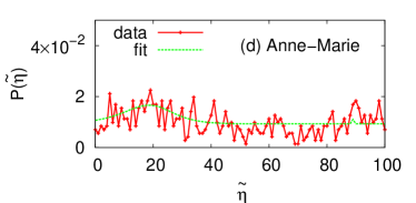
Every year from 1900 to 2000, we randomly sample $2\times 10^{3}$ people out of the corpus and will work with this sampled data henceforth. Otherwise, it would be difficult to compare the number of people given a particular name, counted over the century, with that of another name, because the size of the corpus varies year by year. The resulting $P(\tilde{\eta})$ for the Quebec female names shows four representative types: The first is negatively skewed as depicted in Fig. 3(a), and this comprises the major part of the hundred names. We have found negative skewness for about $60$ names, and the actual number could well be greater than this, because very old or new names show only one of the tails in their time series so that their skewness cannot be determined precisely. There are less than ten names that are better described by right-skewed distribution [Fig. 3(b)]. Only a couple of names exhibit such recurrent behavior [Fig. 3(c)] as has been considered in Ref. Kessler et al., 2012. Note that the recurrence is entirely ignored in our model. Finally, we find three names that are noisy around their respective mean values, and thus not covered by any of the categories above [Fig. 3(d)].

The sampled data points are fitted to our model curve, integrated from Eq. (15). The objective is to minimize the following cost function:

$$\chi^{2}=\sum_{i}\frac{(n_{i}-Np_{i})^{2}}{Np_{i}},$$ (20)

where $n_{i}$ is the number of people given a particular name at year $i$, $N$ is the total number of people given this name over the period from 1900 to 2000, and $p_{i}$ is the predicted fraction from our model. We interpret this problem as distributing $N$ people into 101 bins from 1900 to 2000. We should have four fitting parameters, two of which are $v$ and $g$, and the other two determine translation and scaling along the horizontal axis. We have added one more for a vertical shift, because the $\chi^{2}$ statistic [Eq. (20)] is too sensitive to background noise: Our model describes how a fad of a name catches on and fades away over a certain period, so it has $p_{i}\approx 0$ outside that period. In practice, however, the name can still be found as a stochastic effect. If $p_{i}$ is vanishingly small there, the cost function $\chi^{2}$ diverges. If the noisy fluctuations are not taken into account, therefore, the fitting program will try to avoid this divergence at every cost, even if it misses the main signal. The number of degrees of freedom thus amounts to $d_{f}=101-1-5=95$. The rule of thumb is that $\chi^{2}$ should be of $O(d_{f})$. The conventional criteria for statistical significance allow $\chi^{2}$ to be roughly as high as $130$, which is observed with probability $0.01$ in the $\chi^{2}$ distribution.

Figure 4: (Color online) Monte Carlo fitting results with the Metropolis algorithm. The energy function is identified with $\chi^{2}$ and the temperature is set to be $T=1$. (a) The distribution of $\chi^{2}$ [Eq. (20)] for the hundred female names after the fitting. The vertical line means $\chi^{2}=130$, below which the statistical significance is greater than $0.01$. (b) Distribution of $v$ and $g$ for the names fitted with $\chi^{2}<130$. The error bars express the ranges of the parameters during $10^{5}$ Monte Carlo steps. Inset: A zoomed view. The dotted lines represent $v_{\rm min}=\sqrt{4g+2}$. (c) Estimated $v$ and $g$ against the mean time of prevalence [Eq. (1)] for the names in the inset of (b). (d) Actual data and fitting curves for two outliers on the $(g,v)$ plane, indicated by the arrows in (b).

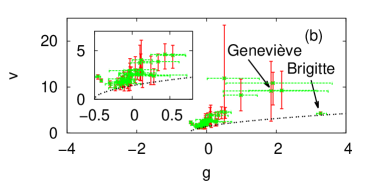
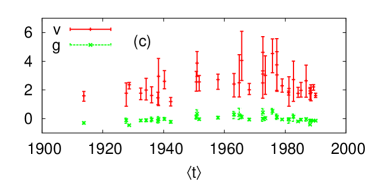
The parameters are adjusted by the Metropolis algorithm, in which Eq. (20) plays the role of the energy function. The energy landscape will be simple enough to apply the zero-temperature Monte Carlo method, as long as the initial condition is reasonably chosen. To estimate the possible ranges of the fitting parameters, however, we choose a finite temperature $T=1$ because fluctuations of $O(1)$ in $\chi^{2}$ will hardly affect the statistical significance. The initial parameters for translation and scaling can be estimated by checking the statistical moments of the data, and we try two initial values of $g=0$ and $g=0.4$, with $v=v_{\rm min}(g)$, for faster convergence. The resulting distribution of $\chi^{2}$ for the hundred female names is plotted in Fig. 4(a). The figure shows that about 40 percents of the hundred female names are successfully described by our model, yielding $\chi^{2}\lesssim 130$. For these names, we also plot the ranges of their fitting parameters in Fig. 4(b). Here, one immediately finds a cluster of names with $g\approx 0$ and $v\lesssim 5$, which is separately depicted in the inset. We see from this figure that many of the parameter values do overlap as predicted by our theory. It is also interesting that the estimated speed is not far from $v_{\rm min}$, if we consider that a new fad would start with a sharp initial condition. Figure 4(c) shows the estimated parameters of the names inside the cluster, against their $\left<t\right>$ [Eq. (1)]. It confirms that the parameters have been stationary throughout the period of observation, which is one of our underlying assumptions.

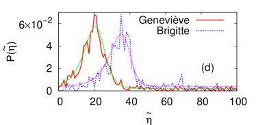
We also have a few outliers that accept fairly large $v$ or $g$. Let us take a closer look by plotting the data for two of them, Geneviève and Brigitte [Fig. 4(d)]. Then, we immediately find that the large $v$ of the former name is likely to be an artifact due to the steady noise level, because a broader distribution may be interpreted as faster propagation (see Appendix B). The same explanation applies to all the other names with large error bars in Fig. 4(b). On the other hand, the latter case of Brigitte shows exceptionally large skewness in spite of rather stable parameter estimations [Fig. 4(b)]. Such a distorted shape is probably caused by external factors that our model cannot account for.

Overall, we conclude that our model does explain a part of the observed data, because it describes about 40 names with consistent values of $v$ and $g$. At the same time, the degree of heterogeneity among the given names has turned out to be higher than we expected from Fig. 1.

IV Discussion and Summary

In summary, we have constructed a model to describe a pattern of fads. Our working hypothesis has been that although each fad is unpredictable, the overall pattern tends to repeat itself over and over again. Figure 1 provides a striking indication of this hypothesis, and suggests that the governing dynamics can develop a traveling-wave solution with a well-defined shape. We have built up a mean-field theory of selection and mutation to explain the observation in Fig. 1. The assumption of a traveling-wave solution implies that the time series of every name can be fitted to a single curve if translated horizontally. We have introduced a shape parameter $g$ in addition to the wave speed $v$, and checked whether these parameters give consistent estimates over the hundred time series. Our model must have oversimplified the reality as we all know that the naming dynamics is involved with many accidental factors such as celebrities and mass media. So as long as the theory predicts sensible behavior, the question should be how much these random fluctuations alter the dynamics. Our analysis suggests the existence of the regularity on a qualitative level: Most of the names are described by unimodal left-skewed distribution, which means that it is common to adopt a fad rapidly and then abandon it slowly. Quantitatively, we have found meaningful fitting results for about $40$ names among $100$. Since we have missed more than a half, we also conclude that the heterogeneity is not so negligible as assumed in the theory.

Appendix A Activator-inhibitor model

Reference Zanette, suggests an alternative model to explain the empirical pattern of given names as follows: Consider a particular name and let $P(t)$ and $Q(t)$ be the fraction of couples that give the name to their babies and the fraction of people that bear the name at time $t$, respectively. The former fraction of couples ‘activate’ the use of this name, whereas the latter fraction of people tend to ‘inhibit’ it. If $\kappa(t)$ means the mortality rate at $t$, the change of $Q(t)$ over a time scale $\tau$ can be written as

$$\frac{d}{dt}Q(t)=\tau^{-1}P(t)-\kappa(t)Q(t),$$ (21)

with a formal solution:

$$Q(t)=\tau^{-1}e^{-I(t)}\int_{-\infty}^{t}P(t^{\prime})e^{I(t^{\prime})}dt^{\prime}+Q(-\infty)e^{-I(t)},$$ (22)

where $I(t)\equiv\int_{-\infty}^{t}\kappa(t^{\prime})dt^{\prime}$. The second term on the RHS can be discarded by setting the surface term at $t=-\infty$ as zero. On the other hand, the governing equation for $P(t)$ is assumed to be

$$\frac{d}{dt}P(t)=-\alpha P^{l}(t)+\beta\left[1-\frac{P(t)}{P_{s}}\right]\left[1-\frac{Q(t)}{Q_{s}}\right]P(t),$$ (23)

where $\alpha$, $\beta$, $l$, $P_{s}$, and $Q_{s}$ are model parameters. The first term on the RHS describes a threshold effect, and $P_{s}$ and $Q_{s}$ mean saturation levels for $P$ and $Q$, respectively.

In this appendix, we compare this activator-inhibitor model with our approach. Let us first assume that the threshold phenomena are negligible and that $P\ll P_{s}$ all the time. Then, the equation simplifies to

$$\frac{d}{dt}P(t)=\beta\left[1-\frac{Q(t)}{Q_{s}}\right]P(t).$$ (24)

If the mortality rate is small enough within the time scale of observation, we can approximate Eq. (22) as

$$Q(t)\approx\tau^{-1}\int_{-\infty}^{t}P(t^{\prime})dt^{\prime}.$$ (25)

Our model considers a traveling wave of velocity $v>0$ represented by $P(x,t)=P(x-vt)$. It implies that the following integral over time

$$\int_{-\infty}^{t}P(x-vt^{\prime})dt^{\prime}=-v^{-1}\int_{-\infty}^{x-vt}P(x-vt^{\prime})d(x-vt^{\prime})$$ (26)

is related to the cumulative distribution

$$C(x-vt)=\int_{-\infty}^{x}P(x^{\prime}-vt)dx^{\prime}=\int_{-\infty}^{x-vt}P(x^{\prime}-vt)d(x^{\prime}-vt).$$ (27)

Roughly speaking, therefore, it is $1-C(x,t)$ that plays the role of inhibition from those who bear the name in our model. Plugging this into Eq. (25), we see that the increase of $P$ is proportional to $C$, which can be written as

$$\frac{\partial P}{\partial t}=k\left(C-\left<C\right>\right)P,$$ (28)

where $k$ is a proportionality constant, and we need $\left<C\right>=\int_{-\infty}^{\infty}C(x^{\prime},t)P(x^{\prime},t)dx^{\prime}$ in the parentheses to guarantee the conservation of total probability $\int_{-\infty}^{\infty}P(x^{\prime},t)dx^{\prime}=1$. The constant $k$ can be absorbed into $t$ by rescaling the time scale. Reference Baek et al., 2013 shows that Eq. (28) has a solution

$$C(x,t)=\frac{1}{2}\tanh\left[h(x)-\frac{t}{4}\right]+\frac{1}{2}$$ (29)

with a certain function $h(x)$ such that $dh/dx\geq 0$, $h(x\rightarrow+\infty)=+\infty$, and $h(x\rightarrow-\infty)=-\infty)$. If this is a traveling wave with a constant velocity, $h(x)$ should be a linear function and $P(x,t)$ thus has a peak with zero skewness. Reference Baek et al., 2013 has found that we can make it skewed just by adding a diffusive term to the ‘reaction’ between activators and inhibitors that Eq. (28) describes. The present work has generalized this finding by introducing a shape parameter called $g$ to control the skewness. It is straightforward to see that Eq. (28) is obtained from Eq. (8) by taking $g=0$, $k=1$, and $D=0$. The activator-inhibitor model in Ref. Zanette, differs from our reaction-diffusion approach in that it mainly focuses on elaborating the reaction kinetics, e.g., by including threshold and saturation effects for $P$. In contrast to such single-name dynamics, the diffusive process introduces other names to the population, playing a similar role to mutation in biology.

Appendix B Speed selection principle

How fast the traveling wave propagates into a linearly unstable state is one of main concerns when we study a reaction-diffusion system. This is usually known as the front propagation problem. In the context of the original Fisher equation Fisher (1937), the traveling wave describes expansion of a population, whose density is denoted as $u(r,t)$, where $r$ means a one-dimensional real space. Under an assumption that $u$ spreads with keeping a constant shape at an asymptotic speed $v_{\rm as}$ in the large-$t$ limit, $u(r,t)$ can be approximated as $u(r-v_{\rm as}t)$. The speed $v_{as}$ of the nonlinear wave is governed by its initial profile at $t=0$ and the leading edge Kolmogorov et al. (1937); Larson (1978); McKean (1975); Rothe (1978); van Saarloos (2003). Let us consider a monotonically decreasing wave profile, such as $u\sim e^{-\zeta r}$. It is known that there is a critical value $\zeta=\zeta^{\ast}$, above which the wave propagates with the lowest speed $v^{\ast}$. Therefore, if the initial profile is steeper than $e^{-\zeta^{\ast}r}$, the wave moves forward at the asymptotic speed $v_{as}$ equal to $v^{\ast}$. Otherwise, it travels at $v_{as}$ larger than $v^{\ast}$, and $v_{as}$ is controlled by the dynamics of the edge which is obtained by linearizing the original equation.

In our notation, $1-C$ maps to the population density $u$ in the Fisher equation. As far as a well-mixed population is concerned, the spatial dependency is negligible and we have $u(r,x,t)=u(x,t)$. For finding the minimum propagation speed $v^{\ast}$, let us substitute $u=1-C$ into Eq. (12) to obtain

$$\frac{\partial u}{\partial t}=\frac{1}{2}u(1-u)(1+2g-2u)+\frac{\partial^{2}u}{\partial x^{2}}.$$ (30)

Equation (30) is linearized at the edge ($u\ll 1$), which results in

$$\frac{\partial u}{\partial t}=\frac{1}{2}u(1+2g)+\frac{\partial^{2}u}{\partial x^{2}}.$$ (31)

Suppose that the wave profile has an exponential tail in the $x$ space, i.e., $u(x,t)=u(x-vt)\sim e^{-\zeta(x-vt)}$. If we plug this ansatz into Eq. (31), it yields a quadratic equation for $\zeta$:

$$\zeta^{2}-v\zeta+\frac{1}{2}(1+2g)=0.$$ (32)

Solving this equation, one obtains a dispersion relation for the edge speed as a function of $\zeta$ as follows:

$$v(\zeta)=\zeta+\frac{1}{2\zeta}(1+2g).$$ (33)

This expression diverges as $\zeta\rightarrow 0$ or $\zeta\rightarrow\infty$ and always has a minimum at $\zeta^{\ast}$ between the two regimes. The derivative of Eq. (33) with respect to $\zeta$ vanishes at such $\zeta^{\ast}$:

$$\frac{\partial v(\zeta)}{\partial\zeta}=1-\frac{1+2g}{\zeta^{2}}=0,$$ (34)

which has two extrema at $\zeta=\pm\sqrt{(1+2g)/2}$. The one with the positive sign gives the minimum speed:

$$v^{\ast}=\sqrt{2(1+2g)}.$$ (35)

Then, $\zeta^{\ast}$ can be expressed self-consistently in terms of $v^{\ast}$, i.e., $\zeta^{\ast}=v^{\ast}/2$.

References

- Camerer (1989) C. Camerer, Journal of Economic Surveys 3, 3 (1989).
- Schaller and van Norden (2002) H. Schaller and S. van Norden, in Advances in Markov-Switching Models, Studies in Empirical Economics, edited by J. Hamilton and B. Raj (Physica Verlag, Heidelberg, 2002) pp. 195–222.
- (3) D. H. Zanette, “Dynamics of fashion: The case of given names,” arXiv:1208.0576.
- Kessler et al. (2012) D. A. Kessler, Y. E. Maruvka, J. Ouren, and N. M. Shnerb, PLOS ONE 7, e38790 (2012).
- Zanette and Manrubia (2001) D. H. Zanette and S. C. Manrubia, Physica A 295, 1 (2001).
- Reed and Hughes (2003) W. J. Reed and B. D. Hughes, Physica A 319, 579 (2003).
- Baek et al. (2007) S. K. Baek, Hoang Ahn Tuan Kiet, and B. J. Kim, Phys. Rev. E 76, 046113 (2007).
- Rossi (2013) P. Rossi, Phys. Life Rev. 10, 395 (2013).
- (9) L. Duchesne, private communication.
- Duchesne (2001) L. Duchesne, Les prénoms. Des plus rares au plus courants au Québec (Éditions du Trécarré, Québec, 2001).
- (11) Institut de la statistique Québec, available at http://www.stat.gouv.qc.ca (accessed 2014 Sep. 22).
- Fisher (1937) R. A. Fisher, Ann. Eugenics 7, 355 (1937).
- Baek et al. (2013) S. K. Baek, X. Durang, and M. Kim, PloS ONE 8, e68583 (2013).
- Kimbrough (1980) S. O. Kimbrough, J. Social Biol. Struct. 3, 149 (1980).
- Orr (2009) H. A. Orr, Nat. Rev. Genet. 10, 531 (2009).
- Taylor and Jonker (1978) P. D. Taylor and L. B. Jonker, Math. Biosci. 40, 145 (1978).
- Hofbauer et al. (1979) J. Hofbauer, P. Schuster, and K. Sigmund, J. Theor. Biol. 81, 609 (1979).
- Maynard Smith (1982) J. Maynard Smith, Evolution and the Theory of Games (Cambridge University Press, Cambridge, 1982).
- Oechssler and Riedel (2001) J. Oechssler and F. Riedel, Econ. Theory 17, 141 (2001).
- Eigen (1971) M. Eigen, Naturwissenschaften 58, 465 (1971).
- Ebeling et al. (1984) W. Ebeling, A. Engel, B. Esser, and R. Feistel, J. Stat. Phys. 37, 369 (1984).
- Zeldovich and Frank-Kamenetsky (1938) Y. B. Zeldovich and D. A. Frank-Kamenetsky, Acta Physicochim 9, 341 (1938).
- Krapivsky et al. (2010) P. L. Krapivsky, S. Redner, and E. Ben-Naim, A Kinetic View of Statistical Physics (Cambridge University Press, Cambridge, 2010).
- Kolmogorov et al. (1937) A. N. Kolmogorov, I. G. Petrovsky, and N. S. Piskunov, Bull. Moscow Univ., Math. Mech. 1, 1 (1937).
- Larson (1978) D. A. Larson, SIAM J. Appl. Math. 34, 93 (1978).
- McKean (1975) H. P. McKean, Comm. Pure Appl. Math. 28, 323 (1975).
- Rothe (1978) F. Rothe, Proc. R. Soc. Edin. A-Ma. 80, 213 (1978).
- van Saarloos (2003) W. van Saarloos, Phys. Rep. 386, 29 (2003).