Persistence in Ferromagnetic Ordering: Dependence upon initial configuration

Abstract

We study the dynamics of ordering in ferromagnets via Monte Carlo simulations of the Ising model, employing the Glauber spin-flip mechanism, in space dimensions $d=2$ and $3$. Results for the persistence probability and the domain growth are discussed for quenches to various temperatures ($T_{f}$) below the critical one ($T_{c}$), from different initial temperatures $T_{i}\geq T_{c}$. In long time limit, for $T_{i}>T_{c}$, the persistence probability exhibits power-law decay with exponents $\theta\simeq 0.22$ and $\simeq 0.18$ in $d=2$ and $3$, respectively. For finite $T_{i}$, the early time behavior is a different power-law whose life-time diverges and exponent decreases as $T_{i}\rightarrow T_{c}$. The crossover length between the two steps diverges as the equilibrium correlation length. $T_{i}=T_{c}$ is expected to provide a new universality class for which we obtain $\theta\simeq 0.035$ in $d=2$ and $\simeq 0.10$ in $d=3$. The time dependence of the average domain size $\ell$, however, is observed to be rather insensitive to the choice of $T_{i}$.

I I Introduction

When a homogeneous system is quenched below the critical point, the system becomes unstable to fluctuations and approaches towards the new equilibrium via the formation and growth of particle rich and particle poor domains onuki_phase ; puri_phase ; bray_phase ; binder_phase . In such nonequilibrium evolutions, over several decades, aspects that received significant attention are the domain pattern bray_phase ; cross ; OJK ; bray_puri ; toyoki ; das1 , rate of domain growth cross ; LS ; bind_stauf ; allen_cahn ; siggia ; huse ; suman1 , persistence satya_1 ; satya_2 ; derrida_1 ; derrida_2 ; manoj ; jkb ; saha and aging d_fisher ; liu ; corberi_1 ; ahmad ; suman_prl ; midya . Average size, $\ell$, of domains typically grows with time ($t$) as cross

$$\ell\sim t^{\alpha}.$$ (1)

The value of the exponent $\alpha$ for nonconserved order-parameter dynamics cross ; allen_cahn , e.g., during ordering in an uniaxial ferromagnet, is $1/2$, in space dimension $d=2$. In addition to the interesting structures exhibited by the domains of like spins (or atomic magnets) in a ferromagnet, the unaffected or persistent spins also form beautiful fractal patterns satya_1 ; satya_2 ; derrida_1 ; derrida_2 ; manoj ; jkb . Typically, fraction of such spins, henceforth will be referred to as the persistent probability, $P$, decays as

$$P\sim t^{-\theta},$$ (2)

with manoj ; stauffer $\theta$ having a value $\simeq 0.22$ for the Ising model in space dimension $d=2$ and $\simeq 0.18$ in $d=3$.

The values of the exponents mentioned above are understood to be true for the perfectly random initial configurations, mimicking the paramagnetic phase at temperature $T=\infty$. Another relevant situation is to quench a system from finite initial temperature ($T_{i}$) with a large enough equilibrium correlation length $\xi$. However, this problem has received only occasional attention dasgupta ; humayun ; newman ; blanchard , though experimentally very relevant. In this context, the behavior of the two-time equal point correlation function, relevant in the aging phenomena, was studied humayun ; newman in $d=2$ for $T_{i}=T_{c}$, the critical temperature. It was pointed out that such quenches would form a new universality class and was shown that the decay of the above correlation was significantly slower for $T_{i}=T_{c}$ than $T_{i}=\infty$. In view of that a slower decay of $P$ is also expected. Apriori, however, it is unclear whether there will be quantitative similarity between the degree of changes in the two quantities. On the other hand, the behavior of $P$ and $\ell$ are expected to be disconnected leticia . Nevertheless, the rate of growth of $\ell$ may be different for $T_{i}=T_{c}$ and $T_{i}=\infty$, at least during the transient period. In this paper, we address the $T_{i}$ dependence for persistence and domain growth in a ferromagnet, via Monte Carlo (MC) simulations d_landau of nearest neighbor Ising model d_landau

$$H=-J\sum_{<ij>}S_{i}S_{j};~{}S_{i}=\pm 1,~{}J>0,$$ (3)

in $d=2$ and $d=3$, on square and simple cubic lattices, respectively.

Starting from a high value, as $T_{i}$ approaches $T_{c}$ [$\simeq$ $2.27J/k_{B}$ in $d=2$ or $4.51J/k_{B}$ in $d=3$, $k_{B}$ being the Boltzmann constant], a two-step decay in $P$ becomes prominent, except for $T_{i}=T_{c}$. For the latter, power-law behavior with exponents much smaller than the ones observed for quenches from $T_{i}=\infty$ lives forever. In addition to identifying these facts, a primary objective of the paper is to accurately quantify these decays. For the domain growth, on the other hand, we do not observe a modification to time dependence with the variation of $T_{i}$, almost from the very beginning.

The rest of the paper is organized as follows. In section II we briefly describe the methods. Results from both the dimensions are presented in section III. Section IV concludes the paper with a summary and outlook.

II II Methods

The nonconserved order-parameter dynamics in the MC simulations have been incorporated via the Glauber spin-flip mechanism glauber . In this method, a randomly chosen spin is tried for a change in sign which is accepted according to the standard Metropolis algorithm d_landau . We apply periodic boundary conditions in all directions. Time is expressed in units of MC steps (MCS), each MCS consisting of $L^{d}$ trials, $L$ being the linear dimension of a square box. We have computed $\ell$ from the domain size distribution, $P_{d}(\ell_{d},t)$, as suman1

$$\ell(t)=\int{\ell_{d}P_{d}(l_{d},t)d\ell_{d}},$$ (4)

where $\ell_{d}$ is calculated as the distance between two successive interfaces in any direction. All lengths are expressed in units of the lattice constant $a$. We present the results after averaging over multiple initial configurations. This number ranges from $20$ (for $L=1024$) to $200$ (for $L=400$) in $d=2$ and $10$ (for $L=256$) to $50$ (for $L=64$) in $d=3$. The initial configurations for $T_{i}$ close to $T_{c}$ were carefully prepared via very long runs. At $T_{c}$, depending upon the system size, length of such runs varied between $5\times 10^{6}$ to $10^{8}$ MCS.

III III Results

III.1 A. $d=2$

Figure 1: Upper panels show snapshots during the evolution of the Glauber Ising model with $T_{i}=\infty$, $T_{f}=0$ and $L=512$. The black regions represent domains of up spins. The lower panels show the unaffected spins, marked in black, corresponding to the evolution snapshots above them. These results correspond to $d=2$.

Figure 2: Plots of persistence probability, $P$, vs, time, on a log-log scale, for quenches from $T_{i}=\infty$, with $L=512$, in $d=2$. Four different values of $T_{f}$ are included. The solid line there has a power-law decay with exponent 0.22.

Figure 3: Log-log plots of $P$ vs $t$, for quenches from different values of $T_{i}(\geqslant T_{c})$, to $T_{f}=0$. Continuous lines there correspond to power-law decays with exponents $0.22$ and $0.04$. (b) Instantaneous exponents $\theta_{i}$ are plotted vs $1/\ell$, for the quenches in (a), excluding $T_{i}=T_{c}$ case. Here we have included only the late time behavior. The continuous lines in this figure are linear fits, providing the values of $\theta$ as the ordinate intercepts. All results are from simulations in $d=2$.

Figure 4: (a) Instantaneous exponents $\theta_{i}$ are plotted vs $1/\ell$ for two of the quenches in Fig. 3(a). Here we have focussed on the first step of the decays, exponents for which are obtained from the flat regions, marked by the horizontal solid lines. These values of $\theta$ are plotted, vs $\epsilon=T_{i}-T_{c}$, in the inset of the figure. The continuous line there is a power-law fit (see text). (b) Plots of $P$ vs $t$, for two different system sizes, with $T_{i}=T_{c}$ and $T_{f}=0$. The upper inset shows $\theta_{i}$ vs $1/\ell$ for three different values of $L$. The dashed line in this inset is a linear extrapolation using data in the small $\ell$ region. The $L$-dependent exponents obtained from flat regions of the plots (see the horizontal solid lines) are plotted vs $1/L$ in the lower inset. The solid line there is a linear fit. All results correspond to $d=2$.

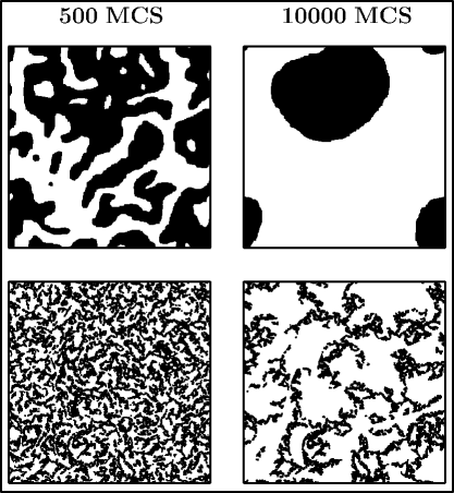
Growth of the domains have been demonstrated in the upper frames of Fig. 1 for the system size $L=512$ in $d=2$. In this figure we show snapshots from two different times during the evolution of the Glauber Ising model. In the lower frames of the figure, we show pictures marking only the persistent spins. Beautiful patterns are visible. These results correspond to a quench from $T_{i}=\infty$ to $T_{f}=0$.

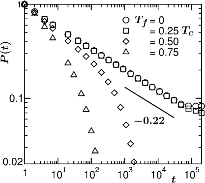
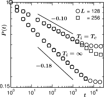
Plots of $P$, for $T_{i}=\infty$ and few different values of $T_{f}$ are shown vs t in Fig. 2. The data for $T_{f}=0$ and $0.25T_{c}$ are consistent with each other and follow power-law, the exponent being $\theta\simeq 0.22$. The flat behavior at the end is due to the finite-size effects. This value of $\theta$ is consistent with the observation by Manoj and Ray manoj . However, for higher values of $T_{f}$, as also previously observed derrida_1 ; derrida_2 , the decay is not of power-law type. This is thought to be due to thermal fluctuation. When this fluctuation is taken care of, we observe $\theta\simeq 0.22$ for all the values of $T_{f}$ included in Fig. 2, in agreement with Ref. [21]. It is thought that persistence and domain growth are not strongly connected to each other. Interestingly, different behavior in Fig. 2 for $T>0.25T_{c}$ is strongly reflected in the domain growth also. For brevity we do not present it here.

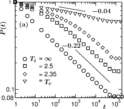
In Fig. 3(a) we show $P$ vs t plots, on a log-log scale, for quenches to $T_{f}=0$, from a few different values of $T_{i}$, all for the same system size $L=512$. It appears that, in the long time limit, for $T_{i}>T_{c}$, the decay is power-law, with the same exponent $\theta\simeq 0.22$. However, crossover to this functional form gets delayed as $T_{i}$ approaches $T_{c}$. In fact, in the pre-crossover regime, another power-law decay, with smaller value of $\theta$, becomes prominent with the decrease of $T_{i}$. Such a slower decay becomes ever-lived for $T_{i}=T_{c}$.

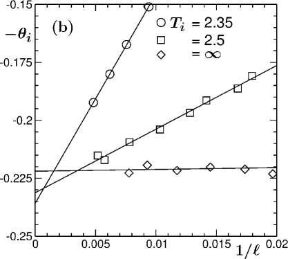
In Fig. 3(b), we present the instantaneous exponent, $\theta_{i}$, calculated as huse ; suman1

$$\theta_{i}=-\frac{d\ln P}{d\ln t},$$ (5)

vs $1/\ell$, with the objective of accurate quantification of the second step of the decays for $T_{i}$ close to, but greater than, $T_{c}$. For the abscissa variable we have adopted $1/\ell$, instead of $1/t$, to visualize the long time limit better. Data sets for each $T_{i}$ are fitted to linear functions to obtain the exponents. Within statistical error, for all the presented temperatures, it appears that $\theta$ is consistent with the quench from $T_{i}=\infty$ to $T_{f}=0$. Nonzero slopes in these plots are due to the presence of off-sets at the crossover times.

Next we move to identify the exponent for $T_{i}=T_{c}$ and $T_{f}=0$. In Fig. 3(a), it appears that the $T_{i}=T_{c}$ data are reasonably consistent with $\theta=0.04$. Nevertheless, before the final finite-size effects appear (showing flat nature at very late time), there is a faster decay, albeit for a brief period. This can well be due to the fact that for a finite system, $\xi$ is not infinite at $T=T_{c}$, effectively implying that the initial configurations are prepared away from $T_{c}$. Thus, in this problem finite-size effects have two sources. One coming from the finiteness of the equilibrium correlation length, other being faced when the nonequilibrium domain size is close to the system size. Thus, a quantification of the exponent $\theta$, for $T_{i}=T_{c}$, via finite-size scaling m_fisher , becomes a challenging task. However, we appropriately take care of the shortcoming below, in various different ways which provide results consistent with each other.

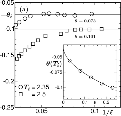
In Fig. 4(a) we show the instantaneous exponents $\theta_{i}$, vs $1/\ell$, with the objective of quantifying the first step of the decay, for two values of $T_{i}$, close enough to $T_{c}$. As demonstrated, from the flat regions we identify the exponents for the early time or the first step of the decay for various values of $T_{i}$. These numbers are plotted in the inset of this figure as a function of $\epsilon=T_{i}-T_{c}$. The continuous line there is a fit to the form

$$\theta(T_{i})=\theta(T_{c})+A\epsilon^{x},$$ (6)

providing $\theta(T_{i}=T_{c})=0.034$, $A=0.15$ and $x=0.54$. Recall that this value of $\theta$ is the only decay exponent for $T_{i}=T_{c}$.

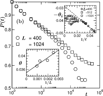
To verify the above value of $\theta$ further, in Fig. 4(b) we present an exercise with different system sizes. In the main frame of this figure, we present $P$ vs $t$ data, for $T_{i}=T_{c}$, from two different values of $L$. It is seen that with the increase of the system size, there is a tendency of the data to settle down to a power-law for a longer period of time, following a marginally faster decay at early time. In the upper inset of this figure we show $\theta_{i}$ vs $1/\ell$ for three different system sizes with $T_{i}=T_{c}$. The early time behavior appears linear, extrapolation of which leads to $\theta\simeq 0.029$. However, if the data in the main frame is closely examined, as already mentioned above, this part corresponds to the preasymptotic behavior, thus, should be discarded from the analysis. Actual asymptotic exponents should be extracted from the flat regions of the plots. The numbers obtained from these flat parts, as discussed, differs due to the finite-size effects and thus, should be extrapolated to $L=\infty$ appropriately. These values are plotted in the lower inset as a function of $1/L$. A very reasonable linear fit (see the solid line) is obtained, providing $\theta=0.035$. On the other hand, a nonlinear fit appears to be nearly quadratic providing $\theta=0.037$. From all these exercises we conclude that $\theta(T_{i}=T_{c})=0.035\pm 0.005$. This picture remains true for quenches from $T_{c}$ to nonzero values of $T_{f}$, if thermal fluctuation effects are appropriately taken care of. On this issue of thermal fluctuation, here, as well as for $T_{i}=\infty$, our studies were restricted to only small system sizes.

The decay of the two-time correlation is also of power-law type. For quenches from $T_{i}=T_{c}$, the value of the exponent gets reduced by a factor $\simeq 10$, compared to $T_{i}=\infty$. In the present case the reduction factor is $\simeq 6.3$. While there may be connection between the two phenomena, but a search for matching between the two factors may not be justified. This is because, only spins with odd number of flips are important for the decay of the two-time correlation function.

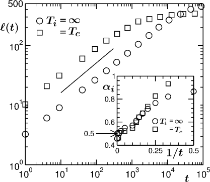
It is certainly important to ask, if, like the decay of the persistence probability and the two-time correlation humayun , the growth of the average domain size also exhibits initial temperature dependence, at least at the transient level. Here we only examine the cases $T_{i}=\infty$ and $T_{i}=T_{c}$, for quenches to $T_{f}=0$. In Fig. 5 we present the $\ell$ vs $t$ plots for these two cases using a log-log scale. Both the data sets appear to grow slower than $t^{1/2}$. This can well be due to the presence of significantly big initial length $\ell_{0}$, which we examine below. While from this figure it is difficult to identify any difference in the growth exponent between the two cases, there certainly exists difference in the finite-size effects, noting that $L=512$ in both the cases.

To learn better about the exponents, in the inset we present the instantaneous exponents huse ; suman1

$$\alpha_{i}=\frac{d\ln\ell}{d\ln t},$$ (7)

with the variation of t. Here, while calculating $\alpha_{i}$, we have subtracted $\ell_{0}$ which are $\simeq 2$ and $\simeq 6.65$, respectively, for $T_{i}=\infty$ and $T_{c}$. This subtraction is meaningful, considering the fact that the pure scaling with respect to time is contained in $\ell-\ell_{0}$. Calculation of $\alpha_{i}$, without such subtraction, provided early time exponents much smaller than the theoretical expectation for the conserved dynamics huse . This has previously been understood to be due to the curvature dependent correction. Such confusion has recently been corrected suman1 . Note that, there may be a delay time for a system to become unstable following a quench. Thus, for an appropriate understanding of a time dependent exponent, the value of $\ell_{0}$ need not be the length at $t=0$. Via finite-size scaling analysis, this was demonstrated in a recent work suman1 . Here, however, we do not undertake such a task.

It may be argued that the value of $\ell_{0}$ should be of the order of system size for $T_{i}=T_{c}$, since $\xi\sim L$ at $T_{c}$. Note here that at criticality fluctuations exist at all length scales. At $T_{i}=T_{c}$, small value of $\ell_{0}$, compared to $L$, is due to the fact that our calculations did not ignore such fluctuations.

First important observation from the inset of Fig. 5 is that the value of $\alpha_{i}$ approaches $1/2$ from the upper side. This is in contradiction with the corresponding behavior for the conserved order parameter dynamics with $T_{f}$ very close to zero suman2 . In the latter case, the early time dynamics provides a growth exponent much smaller than the expected asymptotic value $1/3$. Second, after $t=5$, both the data sets practically follow each other, implying no difference in the growth of $\ell$ almost from the beginning!

Figure 5: Average domain sizes, $\ell(t)$, are plotted vs $t$, for quenches to $T_{f}=0$ from $T_{i}=\infty$ and $T_{c}$, in $d=2$. The solid line represents $t^{1/2}$ behavior. Corresponding instantaneous exponents, vs $1/t$, are shown in the inset. All these results are for $L=512$.

From the length (or time) dependence of $\alpha_{i}$, one can write

$$\alpha_{i}=\alpha+f(1/\ell),$$ (8)

to obtain

$$\int{\frac{d\ell}{{\alpha}l\big{[}1+\frac{1}{\alpha}f(1/\ell)\big{]}}}=\ln t.$$ (9)

If $f(1/\ell)$ can be quantified accurately from the simulation data, a full time dependence of $\ell$ is obtainable. E.g., if $f(1/\ell)$ is a power law, $A_{\beta}/\ell^{\beta}$, $A_{\beta}$ being a constant, by taking ${\alpha}l^{\beta}>A_{\beta}$, one finds

$$\ln\frac{\ell^{1/\alpha}}{t}\sim\frac{1}{{\alpha^{2}}{\beta}{\ell^{\beta}}}.$$ (10)

Assuming that a correction disappears fast, such that $\ell\simeq t^{\alpha}$, we obtain

$$\ell\sim t^{\alpha}\exp(-\frac{C}{{\alpha}{\beta}t^{{\alpha}{\beta}}}),$$ (11)

C being a constant. Such full forms are useful for a finite-size scaling analysis to accurately quantify the exponent $\alpha$. It appears that even for a power-law behavior of $f(1/\ell)$, the asymptotic behavior in the growth law is reached exponentially fast. Of course, from least square fitting exercise of the $\ell$ vs $t$ data also one can aim to obtain the early time corrections. However, this method is more arbitrary. Often derivatives help guessing the functional forms better. We leave the exercise of a finite-size scaling analysis to accurately estimate $\alpha$ and the finite-size effects for a future work.

Before moving on to presenting results in $d=3$, we discuss the issue of persistence again. The essential feature in the initial configurations prepared at different temperatures is the difference in the equilibrium correlation length $\xi$. The basic question, prior to the study, one asks, how the size of $\xi$ affects the decay of persistence probability? For each value of $\xi$, do we have a unique exponent $\theta$ describing the full decay? The answer, as we have observed, is certainly not in affirmative. Essentially, the decay exponent for $T_{i}=\infty$ is recovered for all $\xi$ $(<\infty)$ in the long time limit. The crossover to this asymptotic behavior gets delayed with the increase of $\xi$. It is then natural to ask if this crossover occurs when $\ell$ crosses $\xi$. This can be answered by appropriately estimating the crossover length $\ell_{c}$.

Figure 6: Scaling plot of persistence probability versus $t/t_{c}$ where the crossover time (to the asymptotic behavior) $t_{c}$ has been used as an adjustable parameter to obtain optimum data collapse. Inset: Plots of $\ell_{c}-1$ versus $\epsilon$. The circles correspond to estimates of $\ell_{c}$ from $t_{c}$, the squares are directly obtained from the scaling plots of $P$ vs $\ell/\ell_{c}$. The solid line has $d=2$ Ising critical divergence of correlation length. All results were obtained using $L=512$ in $d=2$.

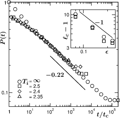
In the main frame of Fig. 6 we show plots of persistence from different values of $T_{i}$, for quenches to $T_{f}=0$. Here the time axis is scaled by appropriate factors (expected to be proportional to cross over time $t_{c}$) to obtain collapse of data in the asymptotic regime. Quality of collapse, on top of the $T_{i}=\infty$ data set, again confirms that $\theta\simeq 0.22$ in the $t\rightarrow\infty$ limit for all $T_{i}$ ($>T_{c}$). From the square roots of these $T_{i}$ dependent scaling factors, one can obtain $\ell_{c}$ which is expected to scale as $\ell_{c}\sim\xi\sim\epsilon^{-\nu}$. Note that for the Ising model $\nu=1$ in $d=2$ and $\simeq 0.63$ in $d=3$. considering that the $T_{i}=\infty$ data have been used as the reference case, it will be appropriate to fit the data set for $\ell_{c}$ to the form

$$\ell_{c}=1+A_{c}\epsilon^{-\nu},$$ (12)

since $\ell_{c}\rightarrow 1$ for $T_{i}=\infty$. Unless we are very close to $T_{c}$ such additional term cannot be neglected. In the inset of Fig. 6 we ahve plotted $\ell_{c}-1$ as a function of $\epsilon$, on a log-log scale. The data set (circles) appear consistent with $\nu=1$. When $\ell_{c}$ is extracted from $t_{c}$, a better exercise requires incorporation of $\ell_{0}$ and growth amplitude for each $T_{i}$. To avoid this problem, we have also obtained $\ell_{c}$ directly from the scaling plots of persistence data vs $\ell/\ell_{c}$ (see the squares). Both data sets appear nicely consistent with each other. In fact, fitting these data to the form in Eq. (12) we obtain $\nu\simeq 0.95$.

III.2 B. $d=3$

Figure 7: Plot of $P$ vs $t$, for quenches from $T_{i}=\infty$ and $T_{i}=T_{c}$, to $T_{f}=0$. In each of the cases results from two different system sizes are included. The solid lines have power-law decays with exponents 0.1 and 0.18, as indicated on the figure. All results corresponds to $d=3$.

Figure 8: Instantaneous exponents $\theta_{i}$ are plotted vs $1/\ell$, for quenches from $T_{i}=T_{c}$ to $T_{f}=0$ in $d=3$. Results from different values of L are included. The horizontal solid lines are related to the estimation of L-dependent $\theta$. Inset: System size dependent $\theta$ are plotted as a function of $1/L$. The continuous line there is a linear fitting (see text for details).

Figure 9: (a) Estimation of $\theta$ for the first step of decay is demonstrated in $d=3$. Inset: Exponent $\theta$ for the first step of the decay is plotted as a function of $\epsilon$, in $d=3$. The continuous line is a non-linear fitting. Further details are provided in the text. (b) Scaling plot of $P$, versus $\ell/\ell_{c}$, in $d=3$. The solid line has a power-law decay with exponent $0.54$. Inset: Plot of $\ell_{c}-1$, in $d=3$, versus $\epsilon$. The solid line there has $d=3$ Ising critical divergence. All results were obtained using $L=128$.

Next we present results in $d=3$. All the important facts being discussed in the previous subsection, here we straightway present the results. Noting that nothing remarkable happened for domain growth in the lower dimension, we stick only to the persistence probability.

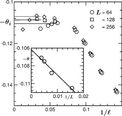
In Fig. 7 we show the $P$ vs $t$ plots for quenches from $T_{i}=\infty$ and $T_{i}=T_{c}$, keeping $T_{f}=0$ in both the cases. For each value of $T_{i}$, results from multiple system sizes are presented. The data for $T_{i}=\infty$ are consistent with $\theta=0.18$, previously reported in stauffer . Thus, here we aim to accurately quantify the value of $\theta$ for $T_{i}=T_{c}$.

Even though, for $T_{i}=T_{c}$, data from both the system sizes in Fig. 7 look consistent with each other, finite-size effects are detectable from a closer look. In the main frame of Fig. 8 we plot $\theta_{i}$ versus $1/\ell$ for a few different values of $L$. Like in $d=2$, from the flat regions we identify system size dependent $\theta$, a plot of which is shown in the inset of this figure. Again, the $\theta$ vs $1/L$ data exhibits a reasonable linear trend and an extrapolation to $L=\infty$ provides $\theta\simeq 0.106$.

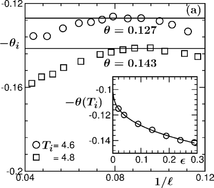
Similar to $d=2$, for $T_{c}<T_{i}<\infty$, two step decays exist in $d=3$ as well. In the main frame of Fig. 9(a) we have demonstrated the estimation of $\theta$ for the first step, for two representative values of $T_{i}$. In the inset of Fig. 9(a) we have plotted these exponents as a function of $\epsilon$. A fit of this data set to the form in Eq. (6) provides $\theta(T_{i}=T_{c})=0.096$, $A=0.07$ and $x=0.34$. This value of $\theta$ is in good agreement with the one obtained from Fig. 8. Thus, in $d=3$, for $T_{i}=T_{c}$, we quote $\theta=0.10\pm 0.02$. The effect of growing correlation length in the initial configurations certainly appears weaker in this space dimension.

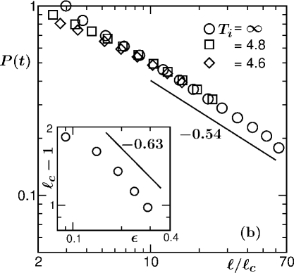
In Fig. 9(b) we show scaling plots of $P$, vs $\ell/\ell_{c}$, using data from different values of $T_{i}$. Collapse of data is good. The late time behavior is power-law and is consistent with a decay exponent $0.54$. Considering that $\theta\simeq 0.18$ in $d=3$, this implies $\alpha=1/3$ in $d=3$ sire . As stated in Ref. [39], deviation of $\alpha$, in this dimension, from $1/2$, is not yet understood. To avoid this, as well as to get rid of the influence of $T_{i}$ dependent $\ell_{0}$ and growth amplitude, we have obtained $\ell_{c}$ from these plots only.

Finally in the inset of Fig. 9(b) we plot $\ell_{c}-1$ as a function of $\epsilon$, on a log-log scale. The divergence of the length scale is consistent with a power law exponent $0.63$ which is the critical exponent for $\xi$ in $d=3$. In fact, a fitting to the form in Eq. (12), excluding the point closest to $T_{c}$, provides $\nu\simeq 0.67$. The reason for the exclusion of the last point is finite-size effect which is clearly visible. Data below $\epsilon=0.1$ are, however, included in the nonlinear fitting in the inset of Fig. 9(a). This is the reason for quoting larger error bar in the final value of $\theta$ there.

IV IV Conclusions

In conclusion, we have studied phase ordering dynamics in Ising ferromagnets for various combinations of initial ($T_{i}$) and final ($T_{f}$) temperatures in $d=2$ and $3$. In this work, the primary focus has been on the persistence probability, $P$, and its connection with the growth of average domain size, $\ell$, as well as the equilibrium initial correlation length $\xi$.

Our general observation has been that, irrespective of the value of $T_{i}$, the decay of $P$ becomes faster with the increase of $T_{f}$, after a certain critical number for the latter. This is understood to be due to spins affected by thermal fluctuations. When this effect is taken care of derrida_2 , the long time decay appears to be power law with exponent manoj ; stauffer consistent with the one for quench to $T_{f}=0$.

As $T_{i}$ approaches $T_{c}$, two-step power-law decay becomes prominent, the second part having exponent $\theta\simeq 0.22$ in $d=2$ and $\simeq 0.18$ in $d=3$, same as $T_{i}=\infty$ and $T_{f}=0$ case. For $T_{i}=T_{c}$, thought to provide a new universality class, the first part of the two-step process lives for ever. The corresponding values of the exponent have been identified to be $\simeq 0.035$ in $d=2$ and $\simeq 0.10$ in $d=3$. Thus, even though, the decay of persistence probability is disconnected with the growth of domain length, its behavior is strongly connected with the initial correlation length. It has been shown that the crossover length to the second step of decays diverges as the equilibrium correlation length in both the dimensions. This leads to the question of difference in the fractal dimensions in the pre and post crossover regimes which needs to be looked at carefully.

We have not observed any initial configuration dependence of the growth of the average domain size. This is consistent with a previous study leticia but more explicitly demonstrated here. Essentially, even the transients are not affected due to change in initial temperature. However, stronger finite-size effects are detected for lower values of $T_{i}$. For domain growth, a striking observation is that the early time exponent is much higher than the asymptotic value, despite $T_{f}$ being zero. This is at variance with the conserved order parameter dynamics. These are all interesting new results, requiring appropriate theoretical attention.

In future we will focus on persistence for the conserved order parameter dynamics. For the conserved dynamics, initial temperature dependence of aging and domain growth are also important open problems.

References

- (1) ONUKI A., Phase Transition Dynamics, (Cambridge University Press, Cambridge, 2002).
- (2) PURI S. and WADHAWAN V. , Kinetics of Phase Transitions, (Boca Raton, CRC Press, 2009).
- (3) BRAY A. J., Adv. Phys. 51, 481 (2002).
- (4) BINDER K., in Phase transformation of materials, edited by CAHN R. W., HAASEN P., KRAMER E. J., Mater. Sci. Technol. Vol. 5 (VCH, Weinheim,1991), p. 405.
- (5) CROSS M. C. and HOHENBERG P. C., Rev. Mod. Phys. 65, 851 (1993).
- (6) OHTA T., JASNOW D. and KAWASAKI K., Phys. Rev. Lett. 49, 1223 (1982).
- (7) BRAY A. J. and PURI S., Phys. Rev. Lett. 67, 2670 (1991).
- (8) TOYOKI H., Phys. Rev. B 45, 1965 (1992).
- (9) DAS S. K., PURI S. and CROSS M. C., Phys. Rev. E 64, 46206 (2001).
- (10) LIFSHITZ I. M. and SLYOZOV V. V., J. Phys. Chem. Solids 19, 35 (1961).
- (11) BINDER K. and STAUFFER D., Phys. Rev. Lett. 33, 1006 (1974).
- (12) ALLEN S. M. and CAHN J. W., Acta Metall. 27, 1085 (1979).
- (13) SIGGIA E. D., Phys. Rev. A 20, 595 (1979).
- (14) HUSE D. A., Phys. Rev. B 34, 7845 (1986).
- (15) MAJUMDER S. and DAS S. K., Phys. Rev. E 81, 050102 (2010).
- (16) MAJUMDAR S. N., SIRE C., BRAY A. J. and CORNELL S. J., Phys. Rev. Lett. 77, 2867 (1996).
- (17) MAJUMDAR S. N., BRAY A. J., CORNELL S. J. and SIRE C., Phys. Rev. Lett. 77, 3704 (1996).
- (18) DERRIDA B., HAKIM V. and ZEITAK R., Phys. Rev. Lett. 77, 2871 (1996).
- (19) DERRIDA B., Phys. Rev. E 55, 3705 (1997).
- (20) MANOJ G. and RAY P., Phys. Rev. E 62, 7755 (2000).
- (21) STAUFFER D., Int. J. Mod. Phys. C 8, 361 (1997).
- (22) CHAKRABORTY D. and BHATTACHARJEE J. K., Phys. Rev. E 76, 031117 (2007).
- (23) SAHARAY M. and SEN P., Physica A 318, 243 (2003).
- (24) FISHER D. S. and HUSE D. A., Phys. Rev. B 38, 373 (1988).
- (25) LIU F. and MAZENKO G. F., Phys. Rev. B 44, 9185 (1991).
- (26) CORBERI F., LIPPIELLO E., ZANNETTI M., Phys. Rev. E 74, 041106 (2006).
- (27) AHMAD S., CORBERI F., DAS S. K., LIPPIELLO E., PURI S. and ZANNETTI M., Phys. Rev. E 86, 061129 (2012).
- (28) MAJUMDER S. and DAS S. K., Phys. Rev. Lett. 111, 055503 (2013).
- (29) MIDYA J., MAJUMDER S. and DAS S. K., J. Phys. : Condens. Matter. 26, 452202 (2014).
- (30) DASGUPTA C. and PANDIT R., Phys. Rev. B 33, 4752 (1986).
- (31) HUMAYUN K. and BRAY A. J., J. Phys. A : Math. Gen. 24, 1915 (1991).
- (32) BRAY A. J., HUMAYUN K. and NEWMAN T. J., Phys. Rev. B 43, 3699 (1991).
- (33) BLANCHARD T., CUGLIANDOLO L. F. and PICCO M., J. Stat. Mech: Theory and experiment P12021 (2014). This very recent work was brought to our notice by an anonymous referee. The value obtained by us is extremely close to the conclusion from this study blanchard for triangular lattice. This implies, the lattice structure plays insignificant role.
- (34) SICILIA A., ARENZON J. A., BRAY A. J. and CUGLIANDOLO L. F., Phys. Rev. E 76, 061116 (2007).
- (35) LANDAU D. P. and BINDER K., A Guide to Monte Carlo Simulations in Statistical Physics (Cambridge University Press, Cambridge, 2009).
- (36) GLAUBER R. J., J. Math. Phys. 4, 294 (1963).
- (37) FISHER M. E., in Critical Phenomena, edited by GREEN M. S. (Academic Press, London, 1971).
- (38) MAJUMDER S. and DAS S. K., Phys. Chem. Chem. Phys. 15, 13209 (2013).
- (39) CUEILLE S. and SIRE C., J. Phys. A: Math. Gen. 30, L791 (1997).