The Lindquist-Wheeler formulation of lattice universes

Rex G Liu R.Liu@damtp.cam.ac.uk Trinity College, Cambridge CB2 1TQ, UK, DAMTP, CMS, Wilberforce Road, Cambridge CB3 0WA, UK.
Abstract

This paper examines the properties of ‘lattice universes’ wherein point masses are arranged in a regular lattice on space-like hypersurfaces; open, flat, and closed universes are considered. The universes are modelled using the Lindquist-Wheeler (LW) approximation scheme, which approximates the space-time in each lattice cell by Schwarzschild geometry. Extending Lindquist and Wheeler’s work, we derive cosmological scale factors describing the evolution of all three types of universes, and we use these scale factors to show that the universes’ dynamics strongly resemble those of Friedmann-Lemaître-Robertson-Walker (FLRW) universes. In particular, we use the scale factors to make more salient the resemblance between Clifton and Ferreira’s Friedmann-like equations for the LW models and the actual Friedmann equations of FLRW space-times. Cosmological redshifts for such universes are then determined numerically, using a modification of Clifton and Ferreira’s approach; the redshifts are found to closely resemble their FLRW counterparts, though with certain differences attributable to the ‘lumpiness’ in the underlying matter content. Most notably, the LW redshifts can differ from their FLRW counterparts by as much as 30%, even though they increase linearly with FLRW redshifts, and they exhibit a non-zero integrated Sachs-Wolfe effect, something which would not be possible in matter-dominated FLRW universes without a cosmological constant.

pacs:
98.80.Jk, 98.80.-k, 04.25.D-

I.   Introduction

Modern cosmology is founded upon the so-called Copernican principle, which posits that the universe ‘looks’ on average to be the same regardless of where one is in the universe or in which direction one looks. More formally, the Copernican principle states that Cauchy surfaces of the universe can be admitted that are homogeneous and isotropic, and this symmetry can be expressed mathematically by writing the universe’s metric in the form

ds2=dt2+a2(t)[dr21kr2+r2(dθ2+sin2θdϕ2)],𝑑superscript𝑠2𝑑superscript𝑡2superscript𝑎2𝑡delimited-[]𝑑superscript𝑟21𝑘superscript𝑟2superscript𝑟2𝑑superscript𝜃2superscript2𝜃𝑑superscriptitalic-ϕ2ds^{2}=-dt^{2}+a^{2}(t)\left[\frac{dr^{2}}{1-kr^{2}}+r^{2}\big{(}d\theta^{2}+\sin^{2}\theta\,d\phi^{2}\big{)}\right], (1)

where a(t)𝑎𝑡a(t) is the time-dependent conformal scale factor, and k𝑘k is the curvature constant. The sign of k𝑘k determines whether 3-spaces of constant t𝑡t will be open, flat, or closed, with k<0𝑘0k<0 corresponding to open universes, k=0𝑘0k=0 to flat universes, and k>0𝑘0k>0 to closed universes; one can always re-scale a(t)𝑎𝑡a(t) and k𝑘k such that k=+1𝑘1k=+1, 00, or 11-1 as appropriate, in which case a(t)𝑎𝑡a(t) becomes the radius of curvature for the open and closed universes. This family of metrics is known as the Friedmann-Lemaître-Robertson-Walker (FLRW) metric. For the metric to satisfy the Einstein field equations of general relativity, a(t)𝑎𝑡a(t) must obey the Friedmann equations {IEEEeqnarray}rCl ( ˙aa )^2 &= 13 (8πρ+ Λ) - ka2,
¨aa  = -4π3 (ρ+ 3p ) + Λ3, where ΛΛ\Lambda is the cosmological constant, and ρ𝜌\rho and p𝑝p are the energy density and pressure of the fluid filling the space. For dust-filled Λ=0Λ0\Lambda=0 universes, the relationship between a𝑎a and t𝑡t is given by {IEEEeqnarray}lr a= a02(1 - cosη)t= a02(η- sinη) &   for k¿0,
a= (94a0)1/3t2/3   for k=0,
a= a02(coshη- 1)t= a02(sinhη- η)   for k¡0, as depicted in Fig. 1, where

a0=8πρ03,subscript𝑎08𝜋subscript𝜌03a_{0}=\frac{8\pi\rho_{0}}{3}, (2)

and ρ0subscript𝜌0\rho_{0} is the energy density when a=1𝑎1a=1. In the case of k>0𝑘0k>0, the factor a0subscript𝑎0a_{0} also corresponds to the maximum of a𝑎a.

a𝑎a

t𝑡tRefer to captionclosedflatopen
Figure 1: Plots of a𝑎a versus t𝑡t for open, flat, and closed dust-filled universes.

These FLRW models have had great success in explaining much of the universe’s behaviour, including most notably the Hubble expansion of the universe, the cosmic microwave background (CMB), and baryon acoustic oscillations. Indeed, the underlying assumption of homogeneity and isotropy appears well-supported by precision measurements showing the CMB to be isotropic to within one part in 100,000. Yet recent measurements of redshifts from Type Ia supernovae (SN1a), when fitted to FLRW models, have led to the conclusion that the universe’s expansion is actually accelerating, and to account for this acceleration, cosmologists have had to modify the standard models by introducing some exotic matter, known generally as dark energy. Two of the most-favoured dark energy models are an FLRW model with non-zero cosmological constant ΛΛ\Lambda, which describes a negative-pressure fluid acting repulsively under gravity and permeating the entire universe, and a scalar field theory called quintessence. However attempts to directly observe any exotic matter and determine its nature have so far proven unsuccessful, and some cosmologists have begun to seek other explanations for the SN1a observations, questioning whether there is any need for exotic matter after all.

There has been an intense debate recently over the relative importance of inhomogeneities in influencing cosmological observations (Ellis and Buchert, 2005; Ellis, 2011; Clarkson et al., 2011). In spite of the wide success of FLRW models, observations clearly show that the late, matter-dominated universe is not homogeneous and isotropic except at the coarsest of scales. Instead, matter is distributed predominantly in clusters and superclusters of galaxies with large voids in between. Standard FLRW models ignore such inhomogeneities completely, with proponents arguing that the inhomogeneities’ effects should be small and hence unimportant. Yet others have argued the converse, proposing that inhomogeneities may have non-trivial implications on both the large-scale dynamics of the universe and on cosmological observations themselves; indeed, inhomogeneities may even explain the SN1a data as an apparent acceleration without any need for exotic matter; this apparent acceleration and analogous effects arise as a result of fitting data from an inhomogeneous universe onto a homogeneous model.

Therefore because of the possibly important implications of inhomogeneities to cosmology, there has been much recent effort in trying to quantify their effects. As the actual universe’s structure is far too complicated to model directly, much effort has been focused on studying the effects of inhomogeneities in toy models. Additionally, there has been much debate on whether perturbed FLRW models can adequately capture the inhomogeneities’ non-linear structure (Kolb et al., 2006; Clarkson and Maartens, 2010; Clarkson and Umeh, 2011). Thus a non-perturbative approach is necessary to unambiguously understand inhomogeneities.

Perhaps the simplest inhomogeneous models that can account for all known cosmological observations are the Lemaître-Tolman-Bondi (LTB) models (Mustapha et al., 1997; Célérier and Schneider, 1998; Tomita, 2000a, b; Alnes et al., 2006; Moffat, 2006; Mansouri, 2006; Garcia-Bellido and Haugbølle, 2008; Clifton et al., 2008; Chuang et al., 2008; Alexander et al., 2009; Bolejko and Wyithe, 2009; February et al., 2010). In such models, the observer is located at the centre of a Hubble-scale under-dense region in a spherically-symmetric, dust-dominated universe. These models are therefore isotropic but not homogeneous. What is most noteworthy is that these models can successfully generate the SN1a redshift data without requiring any exotic matter.

FLRW-based inhomogeneous models have also been constructed using the ‘Swiss Cheese’ methodology developed by Einstein and Straus (Einstein and Straus, 1945; *EinsteinStraus-err). In these models, co-moving spheres are excised from FLRW space-times and replaced by either Schwarzschild space-time or LTB space-time (Kantowski, 1969; Biswas and Notari, 2008; Marra et al., 2007; Brouzakis et al., 2008; Marra et al., 2008; Clifton and Zuntz, 2009). The resulting models are still exact solutions to the Einstein field equations. By construction, the fluid region surrounding the excised spheres is still described by the FLRW metric; therefore these models would still be dynamically identical to FLRW. However, there is no a priori reason to believe their optical properties should be the same; nevertheless, studies have shown that they are generally similar though not identical to FLRW (Biswas and Notari, 2008; Marra et al., 2007; Brouzakis et al., 2008; Marra et al., 2008; Clifton and Zuntz, 2009).

In contrast to the above approaches, we shall consider a completely different space-time that is not in any way based on FLRW nor includes any continuous fluid in its matter content. Rather, we shall consider a space-time where the matter content consists solely of discrete point masses with vacuum in between, as this would provide a more realistic description of the late universe’s matter content. However, for simplicity, our space-time will still possess a high degree of symmetry, though not to the extent of the FLRW universes. Specifically, we shall consider the so-called lattice universes where the matter content on each Cauchy surface consists of identical point masses arranged into a regular lattice. We shall focus on lattices constructed by tessellating a 3-space of constant curvature with identical regular polyhedral cells; the possible lattices obtainable from such a tessellation are summarised in Appendix A. To ‘construct’ a lattice universe, one of the lattices in Appendix A is selected, and all mass in each cell is ‘concentrated’ into a point at its centre. The metric consistent with such a matter distribution is expected to be invariant under the same symmetry transformations that leave the lattice invariant, symmetries which include discrete translation symmetries, discrete rotational symmetries, and reflection symmetries at the cell boundaries. In other words, the lattice universe should have a metric of the form

ds2=dt2+γab(3)(t,𝐱)dxadxb,𝑑superscript𝑠2𝑑superscript𝑡2subscriptsuperscript𝛾3𝑎𝑏𝑡𝐱𝑑superscript𝑥𝑎𝑑superscript𝑥𝑏ds^{2}=-dt^{2}+\gamma^{(3)}_{ab}\left(t,\mathbf{x}\right)\,dx^{a}dx^{b}, (3)

where γab(3)(t,𝐱)subscriptsuperscript𝛾3𝑎𝑏𝑡𝐱\mathbf{\gamma}^{(3)}_{ab}\left(t,\mathbf{x}\right) is the 3-dimensional metric for constant t𝑡t hypersurfaces, and Latin indices a,b=1,2,3formulae-sequence𝑎𝑏123a,b=1,2,3 denote spatial co-ordinates only; the spatial metric γab(3)(t,𝐱)subscriptsuperscript𝛾3𝑎𝑏𝑡𝐱\mathbf{\gamma}^{(3)}_{ab}\left(t,\mathbf{x}\right) at constant t𝑡t would possess the lattice symmetries. Effectively, the Copernican symmetries of FLRW universes have been reduced to just these symmetries. Yet these lattice universes still satisfy the Copernican principle in a coarse-grained manner, in contrast to LTB models where homogeneity of the universe is completely surrendered.

There has been some progress towards determining the 3-metric γ(3)(t,𝐱)superscript𝛾3𝑡𝐱\mathbf{\gamma}^{(3)}\left(t,\mathbf{x}\right). For the closed universe, the 3-metric γ(3)(t=0,𝐱)superscript𝛾3𝑡0𝐱\mathbf{\gamma}^{(3)}\left(t=0,\mathbf{x}\right) on the time-symmetric hypersurface was first determined by Wheeler for the 5-cell universe (Wheeler, 1983) and then more recently by Clifton et al. for all closed lattices (Clifton et al., 2012a); this work has been further generalised by Korzyński who examined closed universes with an arbitrary number of identical masses, not necessarily arranged in a lattice (Korzyński, 2014). The time evolution of this initial data has been investigated numerically by Bentivegna and Korzyński (Bentivegna and Korzyński, 2012) and analytically by Clifton et al. (Clifton et al., 2013, 2014); however Clifton et al. only considered the evolution of certain highly-symmetric curves on the initial surface, so the complete, analytic 4-metric of the closed universe is still lacking. The flat lattice universe has been modelled perturbatively by Bruneton and Larena (Bruneton and Larena, 2012) and numerically by various authors (Yoo et al., 2012, 2013; Bentivegna and Korzyński, 2013); using their perturbative model, Bruneton and Larena have also investigated the flat universe’s optical properties (Bruneton and Larena, 2013). Yet in spite of the progress in determining γ(3)(t,𝐱)superscript𝛾3𝑡𝐱\mathbf{\gamma}^{(3)}\left(t,\mathbf{x}\right), a complete, non-perturbative solution for any lattice universe remains elusive. Moreover, similar analyses of the open universe, analytical or numerical, have yet to be performed; and the optical properties of the closed universe have yet to be examined as well.

Since the complete 4-metric for any lattice universe is still unknown, constructing a non-perturbative approximation of it instead may help provide further insights into the universe’s properties. Such an approximation may, for instance, offer qualitative insights into the universe’s dynamics as well as into the behaviour of photons as they propagate along any arbitrary direction; indeed, it would be difficult to propagate photons through any universe without having a full 4-metric, so for this reason, an analytic approximation of the metric would be especially invaluable. In fact, the lattice universe was first studied using one such approximation. In 1957, Lindquist and Wheeler (LW) (Lindquist and Wheeler, 1957; *LW-err; Wheeler, 1964) devised a construction wherein each polyhedral lattice cell was approximated by a spherical cell with Schwarzschild geometry inside. For this approximation to work though, the masses were required to be of such magnitude and separation that the geometry around each could be reasonably approximated by Schwarzschild geometry; for example, should the masses get too close together, the deviation around each mass from Schwarzschild geometry would become too great such that the LW approximation would break down. The original construction, however, was restricted to approximating closed universes. Yet even in this limited case, Lindquist and Wheeler could obtain a scale factor that very closely resembled the scale factor of closed dust-filled FLRW universes. Indeed, the LW scale factor would asymptotically approach the FLRW scale factor as the total number of masses in the universe increased while the universe’s total mass was held constant.

More recently, Clifton and Ferreira (CF) (Clifton and Ferreira, 2009a; *CF-err) have re-visited the LW construction and extended it in several notable ways. First, they were able to generalise the construction so that flat and open universes could be modelled as well. Secondly, while Lindquist and Wheeler had defined a ‘cosmological time’ co-ordinate in the neighbourhood of the cell boundaries, Clifton and Ferreira were able to extend the co-ordinate to cover the entire space-time globally. This opened the way to a definition of co-moving observers for lattice universes, thereby allowing quantities such as cosmological redshifts to be defined. Finally, Clifton and Ferreira were able to define a set of boundary conditions that photons must obey when crossing from one cell into the next, thereby allowing photons to be propagated across the entire LW model. With their extension, Clifton and Ferreira then modelled the flat lattice universe and found that its evolution and redshifts generally agreed well with those of the flat dust-filled FLRW universe but that its angular diameters and luminosity distances differed (Clifton et al., 2012b).

In this paper, we shall further explore the properties of the lattice universe using the LW approximation with the CF extensions. We shall consider all three types of universes, closed, flat, as well as open. First, we shall extend the LW evolution equation for the closed universe’s scale factor and derive analogous expressions for the flat and open universes. These scale factors are related to the radius of the cell boundary by a constant scaling, and in all three cases, the scale factors have the same functional form as their FLRW counterparts in (1)–(1). Secondly, as Clifton and Ferreira have shown, the LW cell boundary radius satisfies a Friedmann-like equation for all three types of lattice universes; they have also shown that a similar equation holds for the closed universe’s scale factor. By using the LW scale factors we derived rather than cell radii, we can make the analogy between the CF Friedmann equation and the FLRW Friedmann equation more salient; specifically, we shall demonstrate that the CF Friedmann equation takes a form essentially identical to (1) for Λ=0Λ0\Lambda=0 and with k𝑘k in the LW case also equalling +11+1, 00, or 11-1 according to whether the universe is open, flat, or closed respectively. Moreover, we find that the density ρ𝜌\rho in the LW case equals a cell’s Schwarzschild mass divided by the spherical volume 4πrb3/34𝜋superscriptsubscript𝑟𝑏334\pi r_{b}^{3}/3 where rbsubscript𝑟𝑏r_{b} is the radius of a cell; thus, the density behaves as if the cell were a Euclidean sphere. Thirdly, the CF global co-ordinate system was found unsuitable for studying closed lattice universes. We shall show that for closed universes, the CF co-ordinates do not actually cover the interior of the cell completely but leave a gap region instead. For this reason, we must adopt an alternative co-ordinate system if we wish to propagate photons through closed universes, and in fact, a suitable system was proposed by Lindquist and Wheeler themselves at the end of their original paper (Lindquist and Wheeler, 1957; *LW-err). Fourthly, though our method for propagating photons across the universe is strongly influenced by Clifton and Ferreira’s approach, we have adopted several modifications to the set of conditions used to propagate photons across cell boundaries; these modifications will be justified in the paper. Finally, we shall examine the redshifts of photons travelling along a range of trajectories in closed, flat, and open universes. So far, redshifts have only been studied in the flat universe using both a perturbative approach (Bruneton and Larena, 2013) and the LW formalism (Clifton and Ferreira, 2009a; Clifton et al., 2012b); redshifts for the closed and open universes currently do not exist anywhere in the literature, so this part of our results is entirely new. We shall show that for all three types of universes, the redshifts behave broadly in the same way as their FLRW counterparts though with certain differences that can be attributed to the inhomogeneities of the lattice. One of our most striking results is that LW redshifts can differ from their FLRW counterparts by as much as 30%, which has implications on estimating the age of the photon’s source, and that an LW universe can give rise to a non-zero integrated Sachs-Wolfe effect without needing any cosmological constant.

This paper is organised as follows. The second section will explain the origins of the LW approximation and detail its construction; the CF generalisation to flat and open universes will also be reviewed. This section will also compare the CF and LW global co-ordinate system and demonstrate the existence of a gap region if the CF system is applied to closed universes. The third section will derive the LW analogues of the FLRW scale factor and the modified CF Friedmann equation for all three types of lattice universes. The latter half of this paper will examine the behaviour of redshifts in the lattice universe. The fourth section will briefly explain the manner by which redshifts are computed, which follows the method of Clifton and Ferreira. The fifth section will explain the boundary conditions that are used to propagate photons across the boundary between two contiguous cells. The sixth section will explain the numerical method used to simulate the propagation of photons through the lattice. We shall apply Williams and Ellis’ Regge calculus formalism for Schwarzschild space-time to each cell (Williams and Ellis, 1981, 1984); however we have derived an improvement to their rules for tracing geodesics through the Williams-Ellis Schwarzschild space-time which significantly enhances numerical accuracy. Our improvement will be derived in this section with supporting numerical evidence presented in Appendix B; the improvement is not specific to the models being considered in this paper but is applicable to any situation where the Williams-Ellis scheme is being used to numerically simulate geodesics through Schwarzschild space-time. The penultimate section presents and analyses the redshift results of our simulations. The final section concludes with a discussion of possible directions in which this work might be extended.

In this paper, we shall use geometric units where G=c=1𝐺𝑐1G=c=1.

II.   Constructing the LW approximation

The LW approximation of lattice universes was inspired by Wigner and Seitz’s (Wigner and Seitz, 1933) method for approximating electronic wavefunctions in crystal lattices. This method approximates the polyhedral cell of a crystal lattice by a sphere of the same volume; any conditions that the wavefunction must satisfy on the original cell boundary get imposed on the spherical boundary instead. For instance in the original lattice, reflection symmetry at the cell boundary means that the wavefunction ΨΨ\Psi of the lowest energy free electron must satisfy 𝐧Ψ=0𝐧Ψ0\mathbf{n}\cdot\nabla\Psi=0 at the boundary, where the vector 𝐧𝐧\mathbf{n} is orthogonal to the boundary; in the Wigner-Seitz approximation, this same vanishing-derivative condition gets imposed instead on the spherical boundary; that is, ΨΨ\Psi must now satisfy Ψ/r=0Ψ𝑟0\partial\Psi/\partial r=0 at the boundary; and this effectively assumes the electron potential within a cell to be spherically symmetric. The higher the symmetries of the original polyhedral cell, the closer the cell resembles a sphere, and the more accurate the results obtained from the Wigner-Seitz models. Indeed when applied to crystals where exact solutions are known, the Wigner-Seitz construction yields very accurate results (Shockley, 1937; von der Lage and Bethe, 1947).

In analogy with the Wigner-Seitz construction, Lindquist and Wheeler approximate each elementary cell of the lattice universe by a spherical cell and the metric inside each cell by the Schwarzschild metric

ds2=(12mr)dt2+dr2(12mr)+r2(dθ2+sin2θdϕ2).𝑑superscript𝑠212𝑚𝑟𝑑superscript𝑡2𝑑superscript𝑟212𝑚𝑟superscript𝑟2𝑑superscript𝜃2superscript2𝜃𝑑superscriptitalic-ϕ2ds^{2}=-\left(1-\frac{2m}{r}\right)dt^{2}+\frac{dr^{2}}{\left(1-\frac{2m}{r}\right)}+r^{2}\left(d\theta^{2}+\sin^{2}\theta d\phi^{2}\right). (4)

They have called this spherical cell the Schwarzschild-cell. Without knowing the true metric, one cannot directly assess how well is a polyhedral cell in the lattice universe approximated by a spherical one. However Lindquist and Wheeler have shown that polyhedra in a closed or flat 3-space of constant curvature are reasonably approximated by spheres of equal volume (Lindquist and Wheeler, 1957; *LW-err; Wheeler, 1964); hence when such polyhedra are combined into lattices in such 3-spaces, the polyhedral lattice cells would be reasonably well-approximated by spherical cells. They therefore provide this as partial evidence that the approximation would probably be reasonable as well for the polyhedral cells in the lattice universe.

In contrast to the Wigner-Seitz lattice, the LW lattice is itself dynamical. A test particle sitting at the boundary between two Schwarzschild-cells will by symmetry always remain at the boundary. Yet like any other test particle in a Schwarzschild geometry, this test particle must also be radially falling towards the centre of one of the Schwarzschild-cells. And by the same reasoning, this particle is also radially falling towards the centre of the other Schwarzschild-cell. Therefore this test particle, and hence the cell boundary itself, is radially falling towards both cell centres simultaneously, as depicted in Fig. 2.

Refer to caption
\begin{picture}(3617.0,1814.0)(893.0,-3818.0)\end{picture}
Figure 2: A test particle co-moving with the boundary between two cells must be simultaneously falling towards both central masses. Thus the boundary itself must expand and contract accordingly.

The boundary’s motion is hence given by the equation of motion for a radial time-like geodesic,

(drdτ)2=E1+2mr,superscript𝑑𝑟𝑑𝜏2𝐸12𝑚𝑟\left(\frac{dr}{d\tau}\right)^{2}=E-1+\frac{2m}{r}, (5)

where τ𝜏\tau is the proper time of a test particle following the geodesic and E𝐸E is a positive constant of motion; it can be shown that E𝐸\sqrt{E} is the particle’s energy per unit mass at radial infinity. However this simultaneous free-fall of the boundary towards the two masses is actually the result of the two masses themselves falling towards each other under their mutual gravitational attraction. This mutual attraction of all the point-masses thereby gives rise to the expansion and contraction of the lattice itself, which manifests as the expansion and contraction of the Schwarzschild-cell boundary.

We can see from (5) that the value of E=Eb𝐸subscript𝐸𝑏E=E_{b} at the boundary determines whether the cell boundaries will expand indefinitely or eventually re-collapse, and hence whether the underlying lattice universe is open, flat, or closed. For Eb<1subscript𝐸𝑏1E_{b}<1, the boundaries will expand until reaching a maximum radius of

rmax=2m1Ebsubscript𝑟𝑚𝑎𝑥2𝑚1subscript𝐸𝑏r_{max}=\frac{2m}{1-E_{b}} (6)

before re-collapsing; this corresponds to a closed universe. For Eb>1subscript𝐸𝑏1E_{b}>1, the boundaries will expand indefinitely; this corresponds to an open universe. And for Eb=1subscript𝐸𝑏1E_{b}=1, the boundaries travel at the escape velocity and just reach radial infinity; this corresponds to a flat universe. Thus it is through this constant Ebsubscript𝐸𝑏E_{b} that Clifton and Ferreira generalise Lindquist and Wheeler’s work to flat and open universes in a natural manner.

Refer to caption
of cell 2t𝑡tΩΩ\Omegar𝑟rr𝑟rt𝑡tΩΩ\OmegaCoordinate patchof cell 1Coordinate patch
Figure 3: Hypersurfaces of constant Schwarzschild time t𝑡t intercept each other rather than mesh together at the cell boundaries. The normals from different cells point in different directions at the boundary. Therefore, Schwarzschild t𝑡t cannot serve as a global cosmological time co-ordinate for our model.
Refer to caption
r𝑟rτ𝜏\taur𝑟rΩΩ\OmegaCoordinate patch

of cell 2

Coordinate patchof cell 1ΩΩ\Omegaτ𝜏\tau
Figure 4: Hypersurfaces of constant τCFsubscript𝜏𝐶𝐹\tau_{\scriptscriptstyle CF} and τLWsubscript𝜏𝐿𝑊\tau_{\scriptscriptstyle LW} mesh at the boundaries, and the normals from the two cells coincide. Therefore either can serve as cosmological time.

In order to ‘glue’ the individual cells together into a lattice, we require that the 3-space of constant time in one Schwarzschild-cell mesh at the boundary with the corresponding 3-space of the neighbouring cell. As Lindquist and Wheeler have pointed out, two 3-spaces will mesh together if and only if they intersect their common boundary orthogonally. Surfaces of constant Schwarzschild time t𝑡t do not satisfy this meshing condition; instead, they intersect each other when they meet, as illustrated in Fig. 4, and some other time co-ordinate must be found.

Both Lindquist and Wheeler as well as Clifton and Ferreira devised new time co-ordinates that satisfied the meshing condition. The LW time co-ordinate is defined for closed universes only while the CF time co-ordinate can only be applied to flat and open universes. Both time co-ordinates are defined to equal the proper times of a congruence of radial time-like geodesics, which must include the geodesics of test particles co-moving with the boundary. Test particles following these geodesics will travel at the same velocity if at the same radius, thus forming freely falling shells. All geodesics’ clocks are calibrated to read identical proper time on some initial space-like hypersurface that intersects the geodesics orthogonally. Then if the congruence was well-chosen, all other constant proper time hypersurfaces will intersect the congruence orthogonally as well. In particular, such hypersurfaces would always intersect the boundary orthogonally, thus satisfying the meshing condition, as illustrated in Fig. 4. Such a definition of time is well-defined globally and can therefore be used as a ‘cosmological time’ parametrising the lattice universe. Such a construction of cosmological time is natural because we expect co-moving cosmological observers to be stationary with respect to constant time hypersurfaces and also to follow freely falling geodesics. However there is no unique choice of congruence; any choice that satisfies our constraints above is acceptable. Thus herein lies the difference between LW time and CF time. Note that (5) actually describes any radial time-like geodesic in Schwarzschild space-time, including boundary geodesics, for which r=rb𝑟subscript𝑟𝑏r=r_{b}. Clifton and Ferreira’s congruence consists of geodesics all having the same constant E𝐸E, namely that of the boundary Ebsubscript𝐸𝑏E_{b}. Lindquist and Wheeler’s congruence uses different E<1𝐸1E<1 for different geodesics. Indeed, it may be possible to find an alternative choice of congruence based on some stronger physical motivation, but we shall not consider this problem here. Instead, we shall use LW time for the closed universe and CF time for the flat and open universes.

For boundaries following out-going trajectories, the CF time co-ordinate τCFsubscript𝜏𝐶𝐹\tau_{\scriptscriptstyle CF} is given by

dτCF=EbdtEb1+2mr(12mr)dr,𝑑subscript𝜏𝐶𝐹subscript𝐸𝑏𝑑𝑡subscript𝐸𝑏12𝑚𝑟12𝑚𝑟𝑑𝑟d\tau_{\scriptscriptstyle CF}=\sqrt{E_{b}}\,dt-\frac{\sqrt{E_{b}-1+\frac{2m}{r}}}{\left(1-\frac{2m}{r}\right)}dr, (7)

where Ebsubscript𝐸𝑏E_{b} is the same positive constant as E𝐸E in (5) for the boundary geodesic. The Schwarzschild metric (4) now becomes

ds2=𝑑superscript𝑠2absent\displaystyle ds^{2}= 1Eb(12mr)dτCF22EbEb1+2mrdτCFdr1subscript𝐸𝑏12𝑚𝑟𝑑superscriptsubscript𝜏𝐶𝐹22subscript𝐸𝑏subscript𝐸𝑏12𝑚𝑟𝑑subscript𝜏𝐶𝐹𝑑𝑟\displaystyle-\frac{1}{E_{b}}\!\left(1-\frac{2m}{r}\right)\!d\tau_{\scriptscriptstyle CF}^{2}-\frac{2}{E_{b}}\sqrt{E_{b}-1+\frac{2m}{r}}d\tau_{\scriptscriptstyle CF}dr (8)
+dr2Eb+r2dΩ2.𝑑superscript𝑟2subscript𝐸𝑏superscript𝑟2𝑑superscriptΩ2\displaystyle{}+\frac{dr^{2}}{E_{b}}+r^{2}d\Omega^{2}.

The boundary’s equation of motion is still given by (5) but with the proper time τ𝜏\tau replaced by τCFsubscript𝜏𝐶𝐹\tau_{\scriptscriptstyle CF}, as it can be shown that τCFsubscript𝜏𝐶𝐹\tau_{\scriptscriptstyle CF} is identical to the boundary’s proper time. In CF co-ordinates, the 4-vector tangent to any trajectory satisfying (5) for E=Eb𝐸subscript𝐸𝑏E=E_{b} is

ua=(1,Eb1+2mr,0,0).superscript𝑢𝑎1subscript𝐸𝑏12𝑚𝑟00u^{a}=\left(1,\sqrt{E_{b}-1+\frac{2m}{r}},0,0\right). (9)

For an arbitrary vector 𝐧𝐧\mathbf{n} tangent to a constant τCFsubscript𝜏𝐶𝐹\tau_{\scriptscriptstyle CF} surface,

na=(0,nr,nθ,nϕ),superscript𝑛𝑎0superscript𝑛𝑟superscript𝑛𝜃superscript𝑛italic-ϕn^{a}=\left(0,n^{r},n^{\theta},n^{\phi}\right), (10)

it can be shown that 𝐮𝐧=0𝐮𝐧0\mathbf{u}\cdot\mathbf{n}=0 and hence that surfaces of constant τCFsubscript𝜏𝐶𝐹\tau_{\scriptscriptstyle CF} are orthogonal to all geodesics satisfying (5) for E=Eb𝐸subscript𝐸𝑏E=E_{b}, including particularly the boundary geodesics. Thus the meshing condition is satisfied, and thus τCFsubscript𝜏𝐶𝐹\tau_{\scriptscriptstyle CF} can serve as a cosmological time.

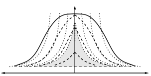
If we attempt to apply the CF co-ordinate system to closed universes though, we encounter problems. When the boundary is contracting, its radial velocity is given by the negative root of (5) instead, and as a result, the square-roots in (7)–(9) must change sign. However the combined co-ordinate patches do not correctly cover the interior of the Schwarzschild-cell. Rather, they leave an uncovered region centred on the boundary’s moment of maximum expansion, as illustrated in Fig. 5.
Refer to caption
r𝑟rr=2M𝑟2𝑀r=2Mt𝑡t
Figure 5: A qualitative plot of various co-moving test-particle trajectories (dashed line) inside a closed Schwarzschild-cell and of various constant τCFsubscript𝜏𝐶𝐹\tau_{\scriptscriptstyle CF} surfaces (dotted line); the plot is of Schwarzschild co-ordinates r𝑟r versus t𝑡t. The cell boundary’s trajectory has been drawn with a solid line. The r𝑟r axis passes through the boundary’s moment of maximum expansion, which happens when τCF=τmaxsubscript𝜏𝐶𝐹subscript𝜏𝑚𝑎𝑥\tau_{\scriptscriptstyle CF}=\tau_{max}. Since the radial velocity must change sign abruptly when the boundary starts closing, there is a noticeable discontinuity in the gradients of the test particle graphs at the r𝑟r axis. The constant τCFsubscript𝜏𝐶𝐹\tau_{\scriptscriptstyle CF} surfaces for τCFsubscript𝜏𝐶𝐹\tau_{\scriptscriptstyle CF} just greater than and less than τmaxsubscript𝜏𝑚𝑎𝑥\tau_{max} are not identical. Between the two surfaces is a ‘gap’ region, shaded in the figure, where space-time points do not have a well-defined cosmological time τCFsubscript𝜏𝐶𝐹\tau_{\scriptscriptstyle CF}.

We shall denote by τmaxsubscript𝜏𝑚𝑎𝑥\tau_{max} the boundary’s proper time at maximum expansion. For τCF<τmaxsubscript𝜏𝐶𝐹subscript𝜏𝑚𝑎𝑥\tau_{\scriptscriptstyle CF}<\tau_{max}, surfaces of constant τCFsubscript𝜏𝐶𝐹\tau_{\scriptscriptstyle CF} are generated by the integral curves of (7) for dτCF=0𝑑subscript𝜏𝐶𝐹0d\tau_{\scriptscriptstyle CF}=0, that is, by

drdt=Eb(12mr)Eb1+2mr>0rbr>2m.formulae-sequence𝑑𝑟𝑑𝑡subscript𝐸𝑏12𝑚𝑟subscript𝐸𝑏12𝑚𝑟0for-allsubscript𝑟𝑏𝑟2𝑚\frac{dr}{dt}=\frac{\sqrt{E_{b}}\left(1-\frac{2m}{r}\right)}{\sqrt{E_{b}-1+\frac{2m}{r}}}>0\qquad\forall\,r_{b}\geq r>2m. (11)

This has a solution of the form t=f(r)+t0𝑡𝑓𝑟subscript𝑡0t=f(r)+t_{0} where t0subscript𝑡0t_{0} is the Schwarzschild time co-ordinate of the surface when it passes through r=r0𝑟subscript𝑟0r=r_{0} and r0subscript𝑟0r_{0} is the Schwarzschild radial co-ordinate satisfying f(r0)=0𝑓subscript𝑟00f(r_{0})=0. Thus on the r𝑟r-t𝑡t plane, like the one shown in Fig. 5, all of these surfaces are identical apart from a horizontal shift corresponding to different t0subscript𝑡0t_{0} constants. Increasing t0subscript𝑡0t_{0} shifts the surface to the right. This implies the surface would intercept the boundary later in the boundary’s trajectory, and therefore τCFsubscript𝜏𝐶𝐹\tau_{\scriptscriptstyle CF} would increase as well. As we keep increasing t0subscript𝑡0t_{0}, we shall eventually reach a limiting surface τCFτmaxsubscript𝜏𝐶𝐹subscript𝜏𝑚𝑎𝑥\tau_{\scriptscriptstyle CF}\to\tau_{max} from the right, and this surface we denote by τmaxsuperscriptsubscript𝜏𝑚𝑎𝑥\tau_{max}^{-}.

For τCF>τmaxsubscript𝜏𝐶𝐹subscript𝜏𝑚𝑎𝑥\tau_{\scriptscriptstyle CF}>\tau_{max}, surfaces of constant τCFsubscript𝜏𝐶𝐹\tau_{\scriptscriptstyle CF} are generated instead by the negative of (11). This has the solution t=f(r)+t0𝑡𝑓𝑟subscript𝑡0t=-f(r)+t_{0}, and again, t0subscript𝑡0t_{0} is the Schwarzschild time co-ordinate of the surface when it passes through r=r0𝑟subscript𝑟0r=r_{0}. On the r𝑟r-t𝑡t plane, all τCF>τmaxsubscript𝜏𝐶𝐹subscript𝜏𝑚𝑎𝑥\tau_{\scriptscriptstyle CF}>\tau_{max} surfaces are also identical to each other apart from a horizontal shift. Decreasing t0subscript𝑡0t_{0} shifts the surface to the left and decreases τCFsubscript𝜏𝐶𝐹\tau_{\scriptscriptstyle CF}. As we decrease t0subscript𝑡0t_{0}, we shall eventually reach a limiting surface τCFτmaxsubscript𝜏𝐶𝐹subscript𝜏𝑚𝑎𝑥\tau_{\scriptscriptstyle CF}\to\tau_{max} from the left, and this surface we denote by τmax+superscriptsubscript𝜏𝑚𝑎𝑥\tau_{max}^{+}.

The complete set of constant τCFsubscript𝜏𝐶𝐹\tau_{\scriptscriptstyle CF} surfaces will completely cover the interior of the cell without any overlaps or gaps if and only if surfaces τmaxsuperscriptsubscript𝜏𝑚𝑎𝑥\tau_{max}^{-} and τmax+superscriptsubscript𝜏𝑚𝑎𝑥\tau_{max}^{+} are identical. This implies that

f(r)+t0𝑓𝑟superscriptsubscript𝑡0\displaystyle f(r)+t_{0}^{-} =f(r)+t0+absent𝑓𝑟superscriptsubscript𝑡0\displaystyle=-f(r)+t_{0}^{+}
f(r)absent𝑓𝑟\displaystyle\implies f(r) =constant,absent𝑐𝑜𝑛𝑠𝑡𝑎𝑛𝑡\displaystyle=constant,

where t0superscriptsubscript𝑡0t_{0}^{-} and t0+superscriptsubscript𝑡0t_{0}^{+} are the t0subscript𝑡0t_{0} constants for τmaxsuperscriptsubscript𝜏𝑚𝑎𝑥\tau_{max}^{-} and τmax+superscriptsubscript𝜏𝑚𝑎𝑥\tau_{max}^{+}, respectively. However we know that function f(r)𝑓𝑟f(r) is not constant, so we have a contradiction.

Instead, we actually have a ‘gap’ between τmaxsuperscriptsubscript𝜏𝑚𝑎𝑥\tau_{max}^{-} and τmax+superscriptsubscript𝜏𝑚𝑎𝑥\tau_{max}^{+}. Both surfaces meet at (τmax,rb(τmax))=(τmax,rmax)subscript𝜏𝑚𝑎𝑥subscript𝑟𝑏subscript𝜏𝑚𝑎𝑥subscript𝜏𝑚𝑎𝑥subscript𝑟𝑚𝑎𝑥\left(\tau_{max},r_{b}(\tau_{max})\right)=(\tau_{max},r_{max}). If we move along τmaxsuperscriptsubscript𝜏𝑚𝑎𝑥\tau_{max}^{-} into the cell, then decreasing r𝑟r would decrease t𝑡t because dr/dt𝑑𝑟𝑑𝑡dr/dt is always positive along this surface. If we move along τmax+superscriptsubscript𝜏𝑚𝑎𝑥\tau_{max}^{+} into the cell, then decreasing r𝑟r would increase t𝑡t because dr/dt𝑑𝑟𝑑𝑡dr/dt is always negative along this surface. On the r𝑟r-t𝑡t plane, τmaxsuperscriptsubscript𝜏𝑚𝑎𝑥\tau_{max}^{-} moves to the left and τmax+superscriptsubscript𝜏𝑚𝑎𝑥\tau_{max}^{+} to the right as r𝑟r decreases from rmaxsubscript𝑟𝑚𝑎𝑥r_{max}. Since τmaxsuperscriptsubscript𝜏𝑚𝑎𝑥\tau_{max}^{-} is the rightmost of the τCF<τmaxsubscript𝜏𝐶𝐹subscript𝜏𝑚𝑎𝑥\tau_{\scriptscriptstyle CF}<\tau_{max} surfaces and τmax+superscriptsubscript𝜏𝑚𝑎𝑥\tau_{max}^{+} the leftmost of the τCF>τmaxsubscript𝜏𝐶𝐹subscript𝜏𝑚𝑎𝑥\tau_{\scriptscriptstyle CF}>\tau_{max} surfaces, the region between τmaxsuperscriptsubscript𝜏𝑚𝑎𝑥\tau_{max}^{-} and τmax+superscriptsubscript𝜏𝑚𝑎𝑥\tau_{max}^{+} is not covered by any τCFsubscript𝜏𝐶𝐹\tau_{\scriptscriptstyle CF} surface and is hence a gap.

We shall therefore use the LW co-ordinate system, which covers closed cells correctly. This system is constructed from a congruence of closed geodesics that attain maximum radii at the same Schwarzschild time. Being a congruence, the geodesics have maximum radii spanning the entire range of 2m<rrb2𝑚𝑟subscript𝑟𝑏2m<r\leq r_{b}, and from a generalised form of (6), the geodesics must therefore have different constants E𝐸E. The geodesics’ clocks are calibrated to have identical proper time at maximum radii. The LW time co-ordinate τLWsubscript𝜏𝐿𝑊\tau_{\scriptscriptstyle LW} at any point is then defined to be the proper time of the geodesic passing through it. Lindquist and Wheeler also defined a new radial co-ordinate r~LWsubscript~𝑟𝐿𝑊\tilde{r}_{\scriptscriptstyle LW} that is constant along each geodesic and equals the geodesic’s maximum radius in Schwarzschild co-ordinates.

The co-ordinate transformation to (τLW,r~LW)subscript𝜏𝐿𝑊subscript~𝑟𝐿𝑊\left(\tau_{\scriptscriptstyle LW},\tilde{r}_{\scriptscriptstyle LW}\right) is then given implicitly by

t=t0±{[(r~LW2m1)(r~LWr)r]1/2+2m(r~LW2m1)1/2(r~LW2m+2)cos1(rr~LW)1/2+2mlnr1/2(r~LW/2m1)1/2+(r~LWr)1/2r1/2(r~LW/2m1)1/2(r~LWr)1/2},\displaystyle\begin{split}t={}&t_{0}\pm\left\{\left[\left(\frac{\tilde{r}_{\scriptscriptstyle LW}}{2m}-1\right)(\tilde{r}_{\scriptscriptstyle LW}-r)r\right]^{1/2}+2m\left(\frac{\tilde{r}_{\scriptscriptstyle LW}}{2m}-1\right)^{1/2}\left(\frac{\tilde{r}_{\scriptscriptstyle LW}}{2m}+2\right)\cos^{-1}\left(\frac{r}{\tilde{r}_{\scriptscriptstyle LW}}\right)^{1/2}\right.\\ &{}\hphantom{t_{0}}+\left.2m\ln\frac{r^{1/2}\left(\tilde{r}_{\scriptscriptstyle LW}/2m-1\right)^{1/2}+\left(\tilde{r}_{\scriptscriptstyle LW}-r\right)^{1/2}}{r^{1/2}\left(\tilde{r}_{\scriptscriptstyle LW}/2m-1\right)^{1/2}-\left(\tilde{r}_{\scriptscriptstyle LW}-r\right)^{1/2}}\right\},\end{split} (12)
τLW=subscript𝜏𝐿𝑊absent\displaystyle\tau_{\scriptscriptstyle LW}={} τ0±(r~LW2m)1/2[r1/2(r~LWr)1/2+r~LWcos1(rr~LW)1/2],\displaystyle\tau_{0}\pm\left(\frac{\tilde{r}_{\scriptscriptstyle LW}}{2m}\right)^{1/2}\left[r^{1/2}\left(\tilde{r}_{\scriptscriptstyle LW}-r\right)^{1/2}+\tilde{r}_{\scriptscriptstyle LW}\cos^{-1}\left(\frac{r}{\tilde{r}_{\scriptscriptstyle LW}}\right)^{1/2}\right], (13)

where t0subscript𝑡0t_{0} and τ0subscript𝜏0\tau_{0} are the time co-ordinates at which the boundary attains its maximum expansion; the positive signs are taken when the boundary is expanding and the negative signs when contracting. The Schwarzschild metric now becomes

ds2=dτLW2+(r~LWr4rr~LW(r~LW/2m1))[(3r~LWr)(rr~LWr)1/2+3r~LWcos1(rr~LW)1/2]2dr~LW2+r2dΩ2,ds^{2}=-d\tau_{\scriptscriptstyle LW}^{2}+\left(\frac{\tilde{r}_{\scriptscriptstyle LW}-r}{4\,r\,\tilde{r}_{\scriptscriptstyle LW}\left(\tilde{r}_{\scriptscriptstyle LW}/2m-1\right)}\right)\left[\left(3\,\tilde{r}_{\scriptscriptstyle LW}-r\right)\left(\frac{r}{\tilde{r}_{\scriptscriptstyle LW}-r}\right)^{1/2}+3\,\tilde{r}_{\scriptscriptstyle LW}\cos^{-1}\left(\frac{r}{\tilde{r}_{\scriptscriptstyle LW}}\right)^{1/2}\right]^{2}d\tilde{r}_{\scriptscriptstyle LW}^{2}+r^{2}\,d\Omega^{2}, (14)

where r𝑟r is now a function of τLWsubscript𝜏𝐿𝑊\tau_{\scriptscriptstyle LW} and r~LWsubscript~𝑟𝐿𝑊\tilde{r}_{\scriptscriptstyle LW}. From this metric, it is clear that surfaces of constant τLWsubscript𝜏𝐿𝑊\tau_{\scriptscriptstyle LW} are always orthogonal to Lindquist and Wheeler’s congruence. Thus the meshing condition is also satisfied, and τLWsubscript𝜏𝐿𝑊\tau_{\scriptscriptstyle LW} is also suitable for use as a cosmological time.

We shall henceforth drop any subscript labels from the cosmological time τ𝜏\tau. In the case of the closed universe, τ𝜏\tau will denote τLWsubscript𝜏𝐿𝑊\tau_{\scriptscriptstyle LW}, while in the flat or open universe, it will denote τCFsubscript𝜏𝐶𝐹\tau_{\scriptscriptstyle CF}.

III.   The cosmological scale factor and the Friedmann equations

There is a clear analogy between the size of the Schwarzschild-cell rb(τ)subscript𝑟𝑏𝜏r_{b}(\tau) and the FLRW scale factor a(t)𝑎𝑡a(t), as both provide a scale of their respective universe’s size. Indeed we expect the lattice universe’s scale factor a(τ)𝑎𝜏a(\tau) should be a function of rbsubscript𝑟𝑏r_{b} alone, that is a(τ)=a(rb(τ))𝑎𝜏𝑎subscript𝑟𝑏𝜏a(\tau)=a(r_{b}(\tau)).111We shall use a(t)𝑎𝑡a(t) when we refer to the FLRW scale factor and a(τ)𝑎𝜏a(\tau) when referring to the lattice universe scale factor. The two functions are completely independent. If we expand rbsubscript𝑟𝑏r_{b}, then each cell of the lattice will expand by some scale ξ𝜉\xi, and therefore the lattice as a whole will expand by ξ𝜉\xi. We shall take a(τ)𝑎𝜏a(\tau) to be related linearly to rb(τ)subscript𝑟𝑏𝜏r_{b}(\tau), that is, a(rb(τ))=αrb(τ)𝑎subscript𝑟𝑏𝜏𝛼subscript𝑟𝑏𝜏a\big{(}r_{b}(\tau)\big{)}=\alpha\,r_{b}(\tau) for some constant α>0𝛼0\alpha>0. As we shall see, a(τ)𝑎𝜏a(\tau) then depends on τ𝜏\tau in a manner analogous to how a(t)𝑎𝑡a(t) depends on t𝑡t for FLRW universes.

Refer to captionξrb𝜉subscript𝑟𝑏\xi r_{b}ξ𝜉\xi\ell\ellrbsubscript𝑟𝑏r_{b}
Figure 6: Rescaling the cell size by ξ𝜉\xi rescales the entire lattice universe by ξ𝜉\xi as well.

Lindquist and Wheeler were able to derive a parametric relationship between a(τ)𝑎𝜏a(\tau) and τ𝜏\tau closely resembling that of (1), thus showing that a(τ)𝑎𝜏a(\tau) behaves essentially identically to its FLRW counterpart a(t)𝑎𝑡a(t); the only difference was the factor of a0subscript𝑎0a_{0}. However, their results were limited to the closed lattice universe. We shall generalise Lindquist and Wheeler’s results, showing that this identical behaviour between a(τ)𝑎𝜏a(\tau) and a(t)𝑎𝑡a(t) holds for lattices of all curvatures. Equation (5) can be integrated to obtain {IEEEeqnarray}rCl τ&= rE2m(r (r_E - r ) + r_E cos^-1rrE  )
            for 0 ¡ E ¡ 1,
τ= (49  rE)^1/2 r^3/2
            for E = 1,
τ= rE2m(r (r_E + r ) - r_E sinh^-1rrE  )
            for E ¿ 1, where

rE={2m|1E|for E1 and E>0,2mfor E=1.subscript𝑟𝐸cases2𝑚1𝐸for 𝐸1 and 𝐸02𝑚for 𝐸1r_{\scriptscriptstyle E}=\begin{dcases}\frac{2m}{\lvert 1-E\rvert}&\text{for }E\neq 1\text{ and }E>0,\\ 2m&\text{for }E=1.\end{dcases} (15)

In the case of E<1𝐸1E<1, rEsubscript𝑟𝐸r_{\scriptscriptstyle E} corresponds to the maximum radius attained by the geodesic, and for the boundary geodesic, where E=Eb𝐸subscript𝐸𝑏E=E_{b}, this maximum radius is identical to (6). For boundary geodesics, where r=rb𝑟subscript𝑟𝑏r=r_{b}, equations (6) to (6) can be re-cast into the form {IEEEeqnarray}ll rb= rEb2(1 - cosη)τ= rEb2rEb2m(η- sinη) &   for 0¡E_b¡1,
rb= (94rEb)1/3τ2/3   for E_b=1,
rb= rEb2(coshη- 1)τ= rEb2rEb2m(sinhη- η)   for E_b¿1, where rEbsubscript𝑟subscript𝐸𝑏r_{\scriptscriptstyle E_{b}} simply denotes rEsubscript𝑟𝐸r_{\scriptscriptstyle E} when E=Eb𝐸subscript𝐸𝑏E=E_{b} and η𝜂\eta is simply a parametrisation. If we choose α𝛼\alpha to be

α=rEb2m,𝛼subscript𝑟subscript𝐸𝑏2𝑚\alpha=\displaystyle\sqrt{\frac{r_{\scriptscriptstyle E_{b}}}{2m}}, (16)

then the scale factor a(τ)𝑎𝜏a(\tau) is given by {IEEEeqnarray}rCll a&= rEb2rEb2m   (1 - cosη)   for 0¡Eb¡1,
a= (94rEbrEb2m )1/3 τ2/3   for Eb¡1,
a= rEb2rEb2m   (coshη- 1)   for Eb¿1. Comparing the relations just obtained for a(τ)𝑎𝜏a(\tau) and τ𝜏\tau with their counterparts in (1)–(1), we find that a(τ)𝑎𝜏a(\tau) and τ𝜏\tau have the same functional form as their FLRW counterparts for all background curvatures. Moreover, we have deduced an expression for the factor α𝛼\alpha that is the same for all universes. The only difference between the lattice and FLRW relations is that a0subscript𝑎0a_{0} for the lattice universe is

a0=rEbrEb2m.subscript𝑎0subscript𝑟subscript𝐸𝑏subscript𝑟subscript𝐸𝑏2𝑚a_{0}=\displaystyle r_{\scriptscriptstyle E_{b}}\sqrt{\frac{r_{\scriptscriptstyle E_{b}}}{2m}}. (17)

Equivalently, by equating (17) with (2), we can say that the density ρ~0subscript~𝜌0\tilde{\rho}_{0} for the lattice universe is

ρ~0=m43πα3.subscript~𝜌0𝑚43𝜋superscript𝛼3\tilde{\rho}_{0}=\frac{m}{\frac{4}{3}\pi\alpha^{-3}}. (18)

The denominator is simply the ‘Euclidean volume’ of a Schwarzschild-cell with radius rbsubscript𝑟𝑏r_{b} corresponding to a=1𝑎1a=1.

As Clifton and Ferreira have noted, the radius of the cell boundary rb(τ)subscript𝑟𝑏𝜏r_{b}(\tau) satisfies an equation strongly resembling the Friedmann equation (1) for Λ=0Λ0\Lambda=0; they also found a similar relation for the closed LW universe’s scale factor. By consistently using the LW scale factors just derived rather than rb(τ)subscript𝑟𝑏𝜏r_{b}(\tau), we can re-express the CF Friedmann equation in a form that makes its resemblance to (1) much more salient; the CF Friedmann equation then becomes

(a˙(τ)a(τ))2=8πρ~3ka(τ)2,superscript˙𝑎𝜏𝑎𝜏28𝜋~𝜌3𝑘𝑎superscript𝜏2\left(\frac{\dot{a}(\tau)}{a(\tau)}\right)^{2}=\frac{8\pi\tilde{\rho}}{3}-\frac{k}{a(\tau)^{2}}, (19)

where k=α2(1Eb)𝑘superscript𝛼21subscript𝐸𝑏k=\alpha^{2}(1-E_{b}) plays the rôle of the curvature constant for the lattice universe, and density ρ~~𝜌\tilde{\rho} is given by

ρ~=m(43πa(τ)3)/α3=m43πrb3.~𝜌𝑚43𝜋𝑎superscript𝜏3superscript𝛼3𝑚43𝜋superscriptsubscript𝑟𝑏3\tilde{\rho}=\frac{m}{\left(\frac{4}{3}\pi a(\tau)^{3}\right)/\alpha^{3}}=\frac{m}{\frac{4}{3}\pi r_{b}^{3}}. (20)

As noted earlier, Ebsubscript𝐸𝑏E_{b} determines whether the universe will be open, flat, or closed, and we see that k𝑘k will take on the correct sign accordingly. In fact, if we make use of (15) and (16), k𝑘k simplifies to 1,0,+1101-1,0,+1 for open, flat, and closed lattice universes, respectively, much like its FLRW analogue.

To complete our model, all that remains is to specify α𝛼\alpha or Ebsubscript𝐸𝑏E_{b}. However, Lindquist and Wheeler have actually provided an argument to specify α𝛼\alpha and an independent argument to effectively222Recall that the quantity Ebsubscript𝐸𝑏E_{b} was introduced to the LW construction afterwards by Clifton and Ferreira. However, Lindquist and Wheeler imposed a tangency condition on the Schwarzschild-cells, which we shall soon describe, that effectively specifies Ebsubscript𝐸𝑏E_{b}. specify Ebsubscript𝐸𝑏E_{b}. What is intriguing is that their choices of α𝛼\alpha and Ebsubscript𝐸𝑏E_{b} are consistent with the relationship between the two quantities required by (16). We shall summarise Lindquist and Wheeler’s arguments leading to their choices. Although they dealt only with closed universes, we shall, in this paper, generalise their arguments to flat and open universes as well.

We begin with Lindquist and Wheeler’s choice of α𝛼\alpha. Note that hypersurfaces of constant t𝑡t in the FLRW metric (1) correspond to 3-spaces of constant curvature, and through an appropriate choice of scaling, the radius of curvature is given by the scale factor a(t)𝑎𝑡a(t). We embed the same type of lattice as the lattice universe on such a hypersurface with the appropriate curvature.333That is, for closed lattice universes, we use hyperspheres; for flat lattice universes, Euclidean space; and for open lattice universes, hyperbolic space. We shall call this hypersurface the comparison hypersurface. We then approximate each polyhedral cell by a sphere of the same volume.444This is actually Clifton and Ferreira’s generalisation. Lindquist and Wheeler’s original condition was that the spheres occupy N1superscript𝑁1N^{-1} of the comparison hypersphere’s total volume, where N𝑁N is the total number of cells. Such a condition clearly needs to be modified for flat and open universes, as both N𝑁N and the hypersurface volume are infinite in these cases. For closed hyperspheres, we define ψ𝜓\psi to be the angle between the centre of the spherical cell and its boundary as measured from the centre of the hypersphere. Then ψ𝜓\psi is given implicitly by

1N=2ψsin2ψ2π,1𝑁2𝜓2𝜓2𝜋\frac{1}{N}=\frac{2\psi-\sin 2\psi}{2\pi}, (21)

where N𝑁N is the total number of cells in the lattice. For hyperbolic spaces, we define ψ𝜓\psi analogously in terms of hyperbolic angles. If r0subscript𝑟0r_{0} is the radius of one such spherical cell, then we can relate r0subscript𝑟0r_{0} to the comparison hypersurface’s radius of curvature aLWsubscript𝑎𝐿𝑊a_{\scriptscriptstyle LW} by

aLW=r0χ(ψ),subscript𝑎𝐿𝑊subscript𝑟0𝜒𝜓a_{\scriptscriptstyle LW}=\frac{r_{0}}{\chi(\psi)}, (22)

where the function χ(ψ)𝜒𝜓\chi(\psi) is given by555Note that when k=0𝑘0k=0 in the FLRW metric (1), we have complete freedom to make a re-scaling of the form rξr𝑟𝜉𝑟r\rightarrow\xi r and aa/ξ𝑎𝑎𝜉a\rightarrow a/\xi. Hence we can always choose a comparison hypersurface such that aLW=r0subscript𝑎𝐿𝑊subscript𝑟0a_{\scriptscriptstyle LW}=r_{0}.

χ(ψ)={sinψfor closed universes,1for flat universes,sinhψfor open universes.𝜒𝜓cases𝜓for closed universes1for flat universes𝜓for open universes\chi(\psi)=\begin{dcases}\sin\psi&\text{for closed universes},\\ 1&\text{for flat universes},\\ \sinh\psi&\text{for open universes}.\end{dcases} (23)

Lindquist and Wheeler identified the Schwarzschild-cell radius rbsubscript𝑟𝑏r_{b} of the lattice universe with r0subscript𝑟0r_{0} and used the corresponding aLWsubscript𝑎𝐿𝑊a_{\scriptscriptstyle LW} as given by (22) to be the lattice universe’s scale factor; that is,

aLW(τ)=rb(τ)χ(ψ).subscript𝑎𝐿𝑊𝜏subscript𝑟𝑏𝜏𝜒𝜓a_{\scriptscriptstyle LW}(\tau)=\frac{r_{b}(\tau)}{\chi(\psi)}. (24)

Hence they have chosen α=1/χ(ψ)𝛼1𝜒𝜓\alpha=1/\chi(\psi). According to (16), Ebsubscript𝐸𝑏E_{b} would therefore correspond to

Eb={cos2ψfor closed universes,1for flat universes,cosh2ψfor open universes.subscript𝐸𝑏casessuperscript2𝜓for closed universes1for flat universessuperscript2𝜓for open universesE_{b}=\begin{dcases}\cos^{2}\psi&\text{for closed universes},\\[2.84526pt] 1&\text{for flat universes},\\[2.84526pt] \cosh^{2}\psi&\text{for open universes}.\end{dcases} (25)

However, Lindquist and Wheeler prescribed Ebsubscript𝐸𝑏E_{b} independently of (16). They instead embedded the Schwarzschild-cell in the comparison hypersurface and required it to be in some sense tangent to the hypersurface. Their prescription for the embedding is as follows. Suppose we replaced each of the original spherical cells in the hypersurface with a Schwarzschild-cell from the lattice universe. Then we want to choose an Ebsubscript𝐸𝑏E_{b} to make the Schwarzschild-cell tangent to the hypersurface. Lindquist and Wheeler formulate this tangency condition as follows. Take any great circle on the boundary of the original sphere and compare its circumference with that of the corresponding great circle on an infinitesimally smaller sphere. Depending on which hypersurface the cell is embedded in, the circumferences will obey the relation

12πd(circumference)d(radial distance)12𝜋𝑑circumference𝑑radial distance\displaystyle\frac{1}{2\pi}\frac{d(\text{circumference})}{d(\text{radial distance})}
={12πd(2πaLWsinψ)aLWdψfor closed hyperspheres,1for flat hypersurfaces,12πd(2πaLWsinhψ)aLWdψfor open hypersurfaces,absentcases12𝜋𝑑2𝜋subscript𝑎𝐿𝑊𝜓subscript𝑎𝐿𝑊𝑑𝜓for closed hyperspheres1for flat hypersurfaces12𝜋𝑑2𝜋subscript𝑎𝐿𝑊𝜓subscript𝑎𝐿𝑊𝑑𝜓for open hypersurfaces\displaystyle\qquad=\begin{dcases}\frac{1}{2\pi}\frac{d(2\pi a_{\scriptscriptstyle LW}\sin\psi)}{a_{\scriptscriptstyle LW}d\psi}&\text{for closed hyperspheres},\\[2.84526pt] 1&\text{for flat hypersurfaces},\\[2.84526pt] \frac{1}{2\pi}\frac{d(2\pi a_{\scriptscriptstyle LW}\sinh\psi)}{a_{\scriptscriptstyle LW}d\psi}&\text{for open hypersurfaces},\end{dcases}
={cosψ,1,coshψ,absentcases𝜓otherwise1otherwise𝜓otherwise\displaystyle\qquad=\begin{dcases}\cos\psi,&\\[2.84526pt] 1,&\\[2.84526pt] \cosh\psi,&\end{dcases}

as depicted by Fig. 9 to Fig. 9. Then for the Schwarzschild-cell to be tangent to the hypersphere, we also require that at its boundary,

12πd(circumference)d(radial distance)={cosψfor closed universes,1for flat universes,coshψfor open universes.12𝜋𝑑circumference𝑑radial distancecases𝜓for closed universes1for flat universes𝜓for open universes\frac{1}{2\pi}\frac{d(\text{circumference})}{d(\text{radial distance})}=\begin{dcases}\cos\psi&\text{for closed universes},\\[2.84526pt] 1&\text{for flat universes},\\[2.84526pt] \cosh\psi&\text{for open universes}.\end{dcases} (26)

From the Schwarzschild metric expressed in CF co-ordinates (8), we can see that d(circumference)=2πdrb𝑑circumference2𝜋𝑑subscript𝑟𝑏d(\text{circumference})=2\pi dr_{b} and that d(radial distance)=drb/Eb𝑑radial distance𝑑subscript𝑟𝑏subscript𝐸𝑏d(\text{radial distance})=dr_{b}/\sqrt{E_{b}}. Thus,

12πd(circumference)d(radial distance)=Eb.12𝜋𝑑circumference𝑑radial distancesubscript𝐸𝑏\frac{1}{2\pi}\frac{d(\text{circumference})}{d(\text{radial distance})}=\sqrt{E_{b}}.

From the Schwarzschild metric in LW co-ordinates (14), it can also be shown, by making use of (13), that (2π)1d(circumference)/d(radial distance)superscript2𝜋1𝑑circumference𝑑radial distance(2\pi)^{-1}d(\text{circumference})/d(\text{radial distance}) is the same. Solving for Ebsubscript𝐸𝑏E_{b}, we then obtain the same result as in (25).

Refer to caption
dψ𝑑𝜓d\psi

aLWdψsubscript𝑎𝐿𝑊𝑑𝜓a_{\scriptscriptstyle LW}d\psi

aLWsinψsubscript𝑎𝐿𝑊𝜓a_{\scriptscriptstyle LW}\sin\psiψ𝜓\psi

aLWsubscript𝑎𝐿𝑊a_{\scriptscriptstyle LW}

Figure 7: A spherical cell of radius aLWsinψsubscript𝑎𝐿𝑊𝜓a_{\scriptscriptstyle LW}\sin\psi and an infinitesimally smaller shell, indicated by the dashed line, have been embedded in a three-dimensional hypersphere of radius aLWsubscript𝑎𝐿𝑊a_{\scriptscriptstyle LW}, with one of the angular dimensions suppressed. The radial distance between the two shells, as measured along the 3-sphere, is aLWdψsubscript𝑎𝐿𝑊𝑑𝜓a_{\scriptscriptstyle LW}d\psi. Because of the curvature of the underlying 3-sphere, we have that d(circumference)/d(radial distance)=2πcosψ𝑑circumference𝑑radial distance2𝜋𝜓d(\text{circumference})/d(\text{radial distance})=2\pi\cos\psi.
Refer to caption
dr𝑑𝑟draLWsubscript𝑎𝐿𝑊a_{\scriptscriptstyle LW}
Figure 8: An analogous embedding in a flat hypersurface. In this case, the circumference of the boundary is 2πaLW2𝜋subscript𝑎𝐿𝑊2\pi a_{\scriptscriptstyle LW}; the radial distance between the two shells is dr𝑑𝑟dr; and d(circumference)/d(radial distance)=2π𝑑circumference𝑑radial distance2𝜋d(\text{circumference})/d(\text{radial distance})=2\pi.
Refer to caption

aLWdψsubscript𝑎𝐿𝑊𝑑𝜓a_{\scriptscriptstyle LW}d\psi

ψ𝜓\psidψ𝑑𝜓d\psiaLWsinhψsubscript𝑎𝐿𝑊𝜓a_{\scriptscriptstyle LW}\sinh\psi
Figure 9: An analogous embedding in a hyperbolic hypersurface. The circumference of the boundary is 2πaLWsinhψ2𝜋subscript𝑎𝐿𝑊𝜓2\pi a_{\scriptscriptstyle LW}\sinh\psi; the radial distance between the two shells is aLWdψsubscript𝑎𝐿𝑊𝑑𝜓a_{\scriptscriptstyle LW}d\psi; and d(circumference)/d(radial distance)=2πcoshψ𝑑circumference𝑑radial distance2𝜋𝜓d(\text{circumference})/d(\text{radial distance})=2\pi\cosh\psi.

We close this section with a few remarks about the large-N𝑁N behaviour of the closed LW model. By taking N𝑁N\to\infty, we can deduce what limiting behaviour the model would approach as the number of masses increases while the universe’s total mass is held constant. It can be shown from (21) that as N𝑁N\to\infty, the angle ψ(3π2N)1/3𝜓superscript3𝜋2𝑁13\psi\to\left(\frac{3\pi}{2N}\right)^{1/3}. If M=Nm𝑀𝑁𝑚M=Nm is the total mass of the universe, then

limNα3m=limNMNsin3ψ=2M3π,subscript𝑁superscript𝛼3𝑚subscript𝑁𝑀𝑁superscript3𝜓2𝑀3𝜋\lim_{N\to\infty}\alpha^{3}\,m=\lim_{N\to\infty}\frac{M}{N\sin^{3}\psi}=\frac{2M}{3\pi},

and therefore the density ρ~0subscript~𝜌0\tilde{\rho}_{0} for the lattice universe, as given by (18), becomes

limNρ~0=M2π2.subscript𝑁subscript~𝜌0𝑀2superscript𝜋2\lim_{N\to\infty}\tilde{\rho}_{0}=\frac{M}{2\pi^{2}}. (27)

In closed FLRW space-time, a hypersphere of constant t𝑡t has a volume of 2π2a(t)32superscript𝜋2𝑎superscript𝑡32\pi^{2}a(t)^{3}. Since the FLRW ρ0subscript𝜌0\rho_{0} is defined to be the density when a(t)=1𝑎𝑡1a(t)=1, then ρ0subscript𝜌0\rho_{0} also equals M/2π2𝑀2superscript𝜋2M/2\pi^{2}. Therefore as N𝑁N\to\infty, the lattice universe density ρ~0subscript~𝜌0\tilde{\rho}_{0} approaches its FLRW equivalent ρ0subscript𝜌0\rho_{0}, and hence the lattice universe factor a0subscript𝑎0a_{0} approaches its FLRW equivalent as well. Consequently, a(τ)𝑎𝜏a(\tau) in (16) approaches a(t)𝑎𝑡a(t) in (1), and τ𝜏\tau in (15) becomes identical to t𝑡t in (1). We also note that ρ~~𝜌\tilde{\rho} in (20) becomes

limNρ~=M2π2a3,subscript𝑁~𝜌𝑀2superscript𝜋2superscript𝑎3\lim_{N\to\infty}\tilde{\rho}=\frac{M}{2\pi^{2}a^{3}}, (28)

which is identical to the FLRW energy density ρ𝜌\rho. This implies that the CF Friedmann equation (19) would be identical to the FLRW Friedmann equation (1) for k=1𝑘1k=1 and Λ=0Λ0\Lambda=0. Therefore, as N𝑁N increases and the closed lattice universe approaches the continuum limit, it becomes increasingly similar to the closed dust-filled FLRW universe, which is consistent with the matter content itself becoming increasingly similar to homogeneous and isotropic dust. In fact, Korzyński has proven that this large-N𝑁N correspondence between the two closed universes is indeed true for the exact solution of the Einstein field equations, at least on the hypersurface of time-symmetry (Korzyński, 2014). He actually considered universes where there could be an arbitrary number N𝑁N of identical Schwarzschild-like black holes and demonstrated that as N𝑁N\to\infty, the hypersurface approaches its FLRW counterpart exactly, both in terms of the scale-factor and in terms of the energy density. Therefore in this regard, the LW approximation agrees with the exact solution.

IV.   Redshifts in the lattice universe

Cosmological redshifts, 1+zFLRW1subscript𝑧𝐹𝐿𝑅𝑊1+z_{\scriptscriptstyle FLRW}, in FLRW universes are defined with respect to sources and observers that are co-moving with the universe’s expansion. The redshifts are given by

1+zFLRW=aoae,1subscript𝑧𝐹𝐿𝑅𝑊subscript𝑎𝑜subscript𝑎𝑒1+z_{\scriptscriptstyle FLRW}=\frac{a_{o}}{a_{e}}, (29)

where aosubscript𝑎𝑜a_{o} and aesubscript𝑎𝑒a_{e} are the cosmological scale factors at the moments of observation and emission, respectively.

We should like to find the lattice universe analogue to zFLRWsubscript𝑧𝐹𝐿𝑅𝑊z_{\scriptscriptstyle FLRW} so that we can compare redshifts in the two types of universes. In general, redshifts 1+z1𝑧1+z are defined as the ratio of the photon frequency measured at the source to the frequency measured by the end observer. The closest analogy to co-moving sources and observers in the lattice universe would be sources and observers that are co-moving with respect to a constant τ𝜏\tau surface. All such observers would be following radial geodesics that obey (5), with E𝐸E fixed to be Ebsubscript𝐸𝑏E_{b} in the flat and open universes but geodesic-dependent in the closed universe. If 𝐮𝐮\mathbf{u} is the 4-velocity of an observer and 𝐤𝐤\mathbf{k} the 4-momentum of a photon as it passes the observer, then the photon frequency measured by the observer would be 𝐮𝐤𝐮𝐤-\mathbf{u}\cdot\mathbf{k}. For the lattice universe, the cosmological redshift is therefore given by

1+zLW=𝐮s𝐤s𝐮o𝐤o,1subscript𝑧𝐿𝑊subscript𝐮𝑠subscript𝐤𝑠subscript𝐮𝑜subscript𝐤𝑜1+z_{\scriptscriptstyle LW}=\frac{\mathbf{u}_{s}\cdot\mathbf{k}_{s}}{\mathbf{u}_{o}\cdot\mathbf{k}_{o}}, (30)

where the subscripts s𝑠s and o𝑜o denote ‘source’ and ‘observer’, respectively. Clifton and Ferreira have constrained their consideration to observers that are co-moving with the photon’s source; that is, at any time τ𝜏\tau, the observer would be at the same radius as the source in their respective cells’ Schwarzschild co-ordinates; this has been illustrated in Fig. 10.

Refer to caption(τf,rf)subscript𝜏𝑓subscript𝑟𝑓(\tau_{f},\;r_{f})(τi,ri)subscript𝜏𝑖subscript𝑟𝑖(\tau_{i},\;r_{i})(τf,rf)subscript𝜏𝑓subscript𝑟𝑓(\tau_{f},\;r_{f})(τi,ri)subscript𝜏𝑖subscript𝑟𝑖(\tau_{i},\;r_{i})
Figure 10: A photon travels from radius risubscript𝑟𝑖r_{i} at cosmological time τisubscript𝜏𝑖\tau_{i} in one cell to radius rfsubscript𝑟𝑓r_{f} at time τfsubscript𝜏𝑓\tau_{f} in the next, as indicated by the long solid arrow. We assume that the photon always passes through the boundary in the manner illustrated here: that is, the point of crossing is a point of tangency between the boundaries of the two cells. A photon is emitted at (τi,ri)subscript𝜏𝑖subscript𝑟𝑖(\tau_{i},\;r_{i}) by a source travelling along a geodesic given by (5) and observed by an observer in another cell. Although in a different cell from the source, the observer is still ‘co-moving’ with the source; that is, for any τ𝜏\tau, the observer is always at the same radius as the source in their respective cells, and this requires the observer to travel along a geodesic with the same E𝐸E as the source.

To facilitate comparison with Clifton and Ferreira’s results, we shall compute redshifts for the same set of observers.

Following Clifton and Ferreira’s example, we shall also use the lattice universe’s scale factor a(τ)𝑎𝜏a(\tau) at the moments of emission and observation to compute zFLRWsubscript𝑧𝐹𝐿𝑅𝑊z_{\scriptscriptstyle FLRW} for comparison; we thus re-express (29) as

1+zFLRW=rb(τo)rb(τe),1subscript𝑧𝐹𝐿𝑅𝑊subscript𝑟𝑏subscript𝜏𝑜subscript𝑟𝑏subscript𝜏𝑒1+z_{\scriptscriptstyle FLRW}=\frac{r_{b}(\tau_{o})}{r_{b}(\tau_{e})}, (31)

where we have made use of the fact that a(τ)=αrb(τ)𝑎𝜏𝛼subscript𝑟𝑏𝜏a(\tau)=\alpha\,r_{b}(\tau).

V.   Propagating photons across cell boundaries

In order to propagate photons through the lattice universe, we must first specify what boundary conditions trajectories must satisfy whenever they pass from one cell into the next. Before discussing the boundary conditions though, we first note a difference between Clifton and Ferreira’s choice of boundary geometry and ours. Clifton and Ferreira converted from spherical cell boundaries back to polyhedral ones, deducing the polyhedral boundary velocity from the requirement that the spherical cell always have the same ‘Euclidean volume’ as the polyhedral cell. We shall instead continue to use spherical boundaries and propagate photons across boundaries in the manner illustrated in Fig. 10; that is, wherever a photon crosses, we always regard the point of crossing as a point of tangency between the two neighbouring cell boundaries. We assume that the boundaries are tangent not just in (3+1)-dimensional space-time as a whole, but also in each 3-dimensional constant-τ𝜏\tau hypersurface, which would be the case had we been using the true polyhedral lattice cells. As Lindquist and Wheeler have argued, spherical boundaries should be a good approximation to the shape of polyhedral boundaries, with the approximation improving as the number of symmetries increases. Therefore any errors due to this approximation would be small to begin with. We further argue that although spherical cells may tile the lattice universe with gaps and overlaps, an arbitrary photon would on average travel through an equal number of gaps and overlaps such that the overall error approximately cancels out, as illustrated in Fig. 11.

Refer to caption
AB
Figure 11: A flat lattice universe with cubic cells approximated by spheres. The central masses are depicted by dots. A photon will on average travel through an equal number of gap and overlap regions. Because we are using spherical boundaries, at boundary crossing A, the photon will jump over a gap region, but at crossing B, it will pass through the overlap twice. The cubic boundaries are tangent to each other everywhere along the boundaries while the spherical boundaries are nowhere tangent to each other except where they intersect; though even there, the tangency is only in the entire (3+1)-dimensional space-time, not in any specific 3-dimensional constant-τ𝜏\tau hypersurface. However in the LW approximation, we shall assume that the spherical boundaries are everywhere tangent to each other, both in the entire (3+1)-dimensional space-time and in each 3-dimensional constant-τ𝜏\tau hypersurface; this is because we are treating the spherical boundaries as if they were approximately identical to the cubic ones.

Additionally, we note that in Clifton and Ferreira’s polyhedral cells, the meshing of constant-τ𝜏\tau hypersurfaces at cell boundaries is lost, with the hypersurfaces now meshing in an average manner only. In contrast, the hypersurfaces in the original spherical cells, by construction, mesh exactly. Finally, the idea of replacing polyhedral boundaries completely with a spherical approximation seems closer in spirit to the original idea of Wigner and Seitz. Therefore according to our choice of boundary geometry, if a photon exits its current cell at a radius r1=rbsubscript𝑟1subscript𝑟𝑏r_{1}=r_{b}, we require it to enter the next cell at radius r2=rbsubscript𝑟2subscript𝑟𝑏r_{2}=r_{b}. Because of cell 2’s spherical symmetry, we are free to choose any θ𝜃\theta and ϕitalic-ϕ\phi co-ordinate for the entry point.

We now present the conditions that photon trajectories must satisfy when propagated across boundaries. These conditions are applied locally at any pair of exit and entry points. Our conditions are founded upon Clifton and Ferreira’s principle that any physical quantity should be independent of which cell’s co-ordinate system an observer co-moving with the boundary may choose to use. In the context of photon trajectories, we require that

  1. 1)

    the photon frequency match across the boundary,

    𝐮1𝐤1=𝐮2𝐤2,subscript𝐮1subscript𝐤1subscript𝐮2subscript𝐤2\mathbf{u}_{1}\cdot\mathbf{k}_{1}=\mathbf{u}_{2}\cdot\mathbf{k}_{2}, (32)
  2. 2)

    and the projection of the photon’s 4-momentum onto the vector 𝐧rsuperscript𝐧𝑟\mathbf{n}^{r} orthogonal to the boundary match across the boundary,666Because of the normalisation condition, this second requirement is equivalent to requiring that the space-like projection of 𝐤𝐤\mathbf{k} onto the boundary be identical in both cells.

    𝐧1r𝐤1=𝐧2r𝐤2;subscriptsuperscript𝐧𝑟1subscript𝐤1subscriptsuperscript𝐧𝑟2subscript𝐤2\mathbf{n}^{r}_{1}\cdot\mathbf{k}_{1}=-\mathbf{n}^{r}_{2}\cdot\mathbf{k}_{2}; (33)

    it can be shown that (nr)a=(0,Eb,0,0)superscriptsuperscript𝑛𝑟𝑎0subscript𝐸𝑏00(n^{r})^{a}=(0,\sqrt{E_{b}},0,0) for both the LW and CF co-ordinate systems. There is a negative sign in the above equation because 𝐧rsuperscript𝐧𝑟\mathbf{n}^{r} always points radially out of its respective cell, whereas the radial direction of 𝐤𝐤\mathbf{k} would be out of one cell and into the next.

These conditions along with the normalisation 𝐤𝐤=0𝐤𝐤0\mathbf{k}\cdot\mathbf{k}=0 are sufficient to deduce the components of 𝐤2subscript𝐤2\mathbf{k}_{2} in terms of 𝐮1subscript𝐮1\mathbf{u}_{1}, 𝐮2subscript𝐮2\mathbf{u}_{2}, and 𝐤1subscript𝐤1\mathbf{k}_{1}.

The vectors 𝐮𝐮\mathbf{u} and 𝐧rsuperscript𝐧𝑟\mathbf{n}^{r} imply a decomposition of 𝐤𝐤\mathbf{k} into the form

𝐤=(𝐤𝐮)𝐮+(𝐤𝐧r)𝐧r+𝐤Ω,𝐤𝐤𝐮𝐮𝐤superscript𝐧𝑟superscript𝐧𝑟superscript𝐤Ω\mathbf{k}=-(\mathbf{k}\cdot\mathbf{u})\mathbf{u}+(\mathbf{k}\cdot\mathbf{n}^{r})\mathbf{n}^{r}+\mathbf{k}^{\Omega}, (34)

where it can be shown that 𝐤Ω𝐮=𝐤Ω𝐧r=0superscript𝐤Ω𝐮superscript𝐤Ωsuperscript𝐧𝑟0\mathbf{k}^{\Omega}\cdot\mathbf{u}=\mathbf{k}^{\Omega}\cdot\mathbf{n}^{r}=0. We note that because of the cell’s spherical symmetry, we can always choose polar co-ordinates such that 𝐤𝐤\mathbf{k} lies in the θ=π/2𝜃𝜋2\theta=\pi/2 plane, thereby allowing us to suppress the θ𝜃\theta co-ordinate. In this case, 𝐤Ωsuperscript𝐤Ω\mathbf{k}^{\Omega} would take the form (kΩ)a=(0,0,0,kΩ)superscriptsuperscript𝑘Ω𝑎000superscript𝑘Ω(k^{\Omega})^{a}=(0,0,0,k^{\Omega}). The above conditions imply that (k1Ω)2=(k2Ω)2superscriptsubscriptsuperscript𝑘Ω12superscriptsubscriptsuperscript𝑘Ω22(k^{\Omega}_{1})^{2}=(k^{\Omega}_{2})^{2}, and by a suitable choice of the ϕitalic-ϕ\phi co-ordinates, we can always make k1Ω=k2Ωsubscriptsuperscript𝑘Ω1subscriptsuperscript𝑘Ω2k^{\Omega}_{1}=k^{\Omega}_{2}. We also note that there is no physical reason for the photon trajectory to refract when passing through a boundary, and therefore the θ=π/2𝜃𝜋2\theta=\pi/2 planes of the two cells should be aligned.

Using the above decomposition and the two boundary conditions, we can therefore express the photon’s 4-momentum 𝐤2subscript𝐤2\mathbf{k}_{2} in the new cell as

𝐤2=(𝐤1𝐮1)𝐮2(𝐤1𝐧1r)𝐧2r+𝐤1Ω.subscript𝐤2subscript𝐤1subscript𝐮1subscript𝐮2subscript𝐤1superscriptsubscript𝐧1𝑟superscriptsubscript𝐧2𝑟superscriptsubscript𝐤1Ω\mathbf{k}_{2}=-(\mathbf{k}_{1}\cdot\mathbf{u}_{1})\mathbf{u}_{2}-(\mathbf{k}_{1}\cdot\mathbf{n}_{1}^{r})\mathbf{n}_{2}^{r}+\mathbf{k}_{1}^{\Omega}. (35)

VI.   Numerical implementation of the LW model

To numerically simulate photons propagating through the lattice universe, we have chosen to implement Williams and Ellis’ Regge calculus scheme (Williams and Ellis, 1981) for Schwarzschild space-times. We shall use their method to discretise the space-time of each Schwarzschild-cell into Regge calculus blocks, and then employ their geodesic-tracing method to propagate photons and test particles through a cell, though with some modifications. In general, the discrete space-times of Regge calculus are expected to converge at second order in the lattice edge-lengths to the continuum space-times of general relativity (Brewin and Gentle, 2001).

Under Willliams and Ellis’ scheme, Schwarzschild space-time is discretised as follows. A grid is constructed in the Schwarzschild space-time such that along any particular gridline, only one Schwarzschild co-ordinate (t,r,θ,ϕ)𝑡𝑟𝜃italic-ϕ(t,r,\theta,\phi) changes while the other three are held constant. The lines intersect at constant ΔtΔ𝑡\Delta t, ΔrΔ𝑟\Delta r, ΔθΔ𝜃\Delta\theta, or ΔϕΔitalic-ϕ\Delta\phi intervals, thus forming the edges of curved rectangular blocks. Each of these blocks gets mapped to flat rectangular Regge blocks such that the straight edges of the Regge blocks have the same lengths as the curved edges of the original blocks; Figure 12 illustrates an example of a curved Schwarzschild block with its corresponding Regge block.

Refer to caption
(ri+1,ϕi,ti+1)subscript𝑟𝑖1subscriptitalic-ϕ𝑖subscript𝑡𝑖1(r_{i+1},\phi_{i},t_{i+1})ϕitalic-ϕ\phir𝑟rt𝑡t(ri+1,ϕi+1,ti)subscript𝑟𝑖1subscriptitalic-ϕ𝑖1subscript𝑡𝑖(r_{i+1},\phi_{i+1},t_{i})(ri,ϕi,ti+1)subscript𝑟𝑖subscriptitalic-ϕ𝑖subscript𝑡𝑖1(r_{i},\phi_{i},t_{i+1})(ri,ϕi+1,ti+1)subscript𝑟𝑖subscriptitalic-ϕ𝑖1subscript𝑡𝑖1(r_{i},\phi_{i+1},t_{i+1})(ri+1,ϕi+1,ti+1)subscript𝑟𝑖1subscriptitalic-ϕ𝑖1subscript𝑡𝑖1(r_{i+1},\phi_{i+1},t_{i+1})(ri+1,ϕi,ti)subscript𝑟𝑖1subscriptitalic-ϕ𝑖subscript𝑡𝑖(r_{i+1},\phi_{i},t_{i})(ri,ϕi,ti)subscript𝑟𝑖subscriptitalic-ϕ𝑖subscript𝑡𝑖(r_{i},\phi_{i},t_{i})(ri,ϕi+1,ti)subscript𝑟𝑖subscriptitalic-ϕ𝑖1subscript𝑡𝑖(r_{i},\phi_{i+1},t_{i})
Refer to caption
(ρi,ψi+1,τi+1)subscript𝜌𝑖subscript𝜓𝑖1subscript𝜏𝑖1(\rho_{i},-\psi_{i+1},\tau_{i+1})τ𝜏\tauψ𝜓\psiρ𝜌\rho(ρi,ψi+1,τi+1)subscript𝜌𝑖subscript𝜓𝑖1subscript𝜏𝑖1(\rho_{i},\psi_{i+1},\tau_{i+1})(ρi,ψi+1,τi+1)subscript𝜌𝑖subscript𝜓𝑖1subscript𝜏𝑖1(\rho_{i},\psi_{i+1},-\tau_{i+1})(ρi,ψi,τi)subscript𝜌𝑖subscript𝜓𝑖subscript𝜏𝑖(-\rho_{i},-\psi_{i},\tau_{i})(ρi,ψi,τi)subscript𝜌𝑖subscript𝜓𝑖subscript𝜏𝑖(-\rho_{i},-\psi_{i},-\tau_{i})(ρi,ψi,τi)subscript𝜌𝑖subscript𝜓𝑖subscript𝜏𝑖(-\rho_{i},\psi_{i},\tau_{i})2di2subscript𝑑𝑖2d_{i}(ρi,ψi+1,τi+1)subscript𝜌𝑖subscript𝜓𝑖1subscript𝜏𝑖1(\rho_{i},-\psi_{i+1},-\tau_{i+1})(ρi,ψi,τi)subscript𝜌𝑖subscript𝜓𝑖subscript𝜏𝑖(-\rho_{i},\psi_{i},-\tau_{i})
Figure 12: On the left is an example of the original Schwarzschild block with one angular co-ordinate suppressed, and on the right is the Regge block to which it is mapped. (τ,ρ,ψ)𝜏𝜌𝜓(\tau,\rho,\psi) is a Minkowski co-ordinate system within the Regge block.

The Schwarzschild co-ordinates of the original blocks’ vertices (ti,rj,θk,ϕl)subscript𝑡𝑖subscript𝑟𝑗subscript𝜃𝑘subscriptitalic-ϕ𝑙(t_{i},r_{j},\theta_{k},\phi_{l}) are now taken over as labels for the Regge blocks’ vertices. As the Regge blocks are flat, the metric inside is simply the Minkowski metric.

Suppose a Regge block had vertices (ti,rj,θk,ϕl)subscript𝑡𝑖subscript𝑟𝑗subscript𝜃𝑘subscriptitalic-ϕ𝑙(t_{i},r_{j},\theta_{k},\phi_{l}) and (ti+1,rj+1,θk+1,ϕl+1)subscript𝑡𝑖1subscript𝑟𝑗1subscript𝜃𝑘1subscriptitalic-ϕ𝑙1(t_{i+1},r_{j+1},\theta_{k+1},\phi_{l+1}); then we shall use the label (ti,rj,θk,ϕl)subscript𝑡𝑖subscript𝑟𝑗subscript𝜃𝑘subscriptitalic-ϕ𝑙(t_{i},r_{j},\theta_{k},\phi_{l}) to refer to this block as a whole. The edge-lengths for this block are

d[(ti,rj,θk,ϕl),(ti+1,rj,θk,ϕl)]𝑑subscript𝑡𝑖subscript𝑟𝑗subscript𝜃𝑘subscriptitalic-ϕ𝑙subscript𝑡𝑖1subscript𝑟𝑗subscript𝜃𝑘subscriptitalic-ϕ𝑙\displaystyle d[(t_{i},r_{j},\theta_{k},\phi_{l}),(t_{i+1},r_{j},\theta_{k},\phi_{l})] =12mrj(ti+1ti),absent12𝑚subscript𝑟𝑗subscript𝑡𝑖1subscript𝑡𝑖\displaystyle=\sqrt{1-\frac{2m}{r_{j}}}\Big{(}t_{i+1}-t_{i}\Big{)},
d[(ti,rj,θk,ϕl),(ti,rj+1,θk,ϕl)]𝑑subscript𝑡𝑖subscript𝑟𝑗subscript𝜃𝑘subscriptitalic-ϕ𝑙subscript𝑡𝑖subscript𝑟𝑗1subscript𝜃𝑘subscriptitalic-ϕ𝑙\displaystyle d[(t_{i},r_{j},\theta_{k},\phi_{l}),(t_{i},r_{j+1},\theta_{k},\phi_{l})] =\bigintssrjrj+1dr12mr,absentsuperscriptsubscript\bigintsssubscript𝑟𝑗subscript𝑟𝑗1𝑑𝑟12𝑚𝑟\displaystyle=\bigintss_{r_{j}}^{r_{j+1}}\mkern-18.0mu\frac{dr}{\sqrt{1-\frac{2m}{r}}},
d[(ti,rj,θk,ϕl),(ti,rj,θk+1,ϕl)]𝑑subscript𝑡𝑖subscript𝑟𝑗subscript𝜃𝑘subscriptitalic-ϕ𝑙subscript𝑡𝑖subscript𝑟𝑗subscript𝜃𝑘1subscriptitalic-ϕ𝑙\displaystyle d[(t_{i},r_{j},\theta_{k},\phi_{l}),(t_{i},r_{j},\theta_{k+1},\phi_{l})] =rj(θk+1θk),absentsubscript𝑟𝑗subscript𝜃𝑘1subscript𝜃𝑘\displaystyle=r_{j}(\theta_{k+1}-\theta_{k}),
d[(ti,rj,θk,ϕl),(ti,rj,θk,ϕl+1)]𝑑subscript𝑡𝑖subscript𝑟𝑗subscript𝜃𝑘subscriptitalic-ϕ𝑙subscript𝑡𝑖subscript𝑟𝑗subscript𝜃𝑘subscriptitalic-ϕ𝑙1\displaystyle d[(t_{i},r_{j},\theta_{k},\phi_{l}),(t_{i},r_{j},\theta_{k},\phi_{l+1})] =rjsinθk(ϕl+1ϕl).absentsubscript𝑟𝑗subscript𝜃𝑘subscriptitalic-ϕ𝑙1subscriptitalic-ϕ𝑙\displaystyle=r_{j}\sin\theta_{k}(\phi_{l+1}-\phi_{l}).

Since photons always move in planes, we can always suppress one of the angular co-ordinates by setting θ𝜃\theta to be π/2𝜋2\pi/2. We then set-up a Minkowski co-ordinate system (τ,ρ,ψ)𝜏𝜌𝜓(\tau,\rho,\psi) in the block, with block vertices located at (±τi,ρi,±ψi)plus-or-minussubscript𝜏𝑖subscript𝜌𝑖plus-or-minussubscript𝜓𝑖(\pm\,\tau_{i},-\rho_{i},\pm\,\psi_{i}) and (±τi+1,ρi,±ψi+1)plus-or-minussubscript𝜏𝑖1subscript𝜌𝑖plus-or-minussubscript𝜓𝑖1(\pm\,\tau_{i+1},\rho_{i},\pm\,\psi_{i+1}), where τisubscript𝜏𝑖\tau_{i}, ρisubscript𝜌𝑖\rho_{i}, and ψisubscript𝜓𝑖\psi_{i} are defined by777Note that an arbitrary index j𝑗j appears in the expressions for τisubscript𝜏𝑖\tau_{i} and ψisubscript𝜓𝑖\psi_{i}. However, because both (tj+1tj)subscript𝑡𝑗1subscript𝑡𝑗(t_{j+1}-t_{j}) and (ϕj+1ϕj)subscriptitalic-ϕ𝑗1subscriptitalic-ϕ𝑗(\phi_{j+1}-\phi_{j}) are actually independent of j𝑗j, it does not matter what value of j𝑗j is used to calculate τisubscript𝜏𝑖\tau_{i} and ψisubscript𝜓𝑖\psi_{i}.

2τi2subscript𝜏𝑖\displaystyle 2\tau_{i} =12mri(tj+1tj),absent12𝑚subscript𝑟𝑖subscript𝑡𝑗1subscript𝑡𝑗\displaystyle=\sqrt{1-\frac{2m}{r_{i}}}\,\Big{(}t_{j+1}-t_{j}\Big{)}, (36)
2ψi2subscript𝜓𝑖\displaystyle 2\psi_{i} =ri(ϕj+1ϕj),absentsubscript𝑟𝑖subscriptitalic-ϕ𝑗1subscriptitalic-ϕ𝑗\displaystyle=r_{i}(\phi_{j+1}-\phi_{j}),
ρisubscript𝜌𝑖\displaystyle\rho_{i} =[di2+(τi+1τi)24(ψi+1ψi)24]1/2,absentsuperscriptdelimited-[]superscriptsubscript𝑑𝑖2superscriptsubscript𝜏𝑖1subscript𝜏𝑖24superscriptsubscript𝜓𝑖1subscript𝜓𝑖2412\displaystyle=\left[d_{i}^{2}+\frac{(\tau_{i+1}-\tau_{i})^{2}}{4}-\frac{(\psi_{i+1}-\psi_{i})^{2}}{4}\right]^{1/2},

and where888In (Williams and Ellis, 1981), there was a missing factor of 2m2𝑚2m in front of the logarithm for this equation; this factor has been restored here.

2di2subscript𝑑𝑖\displaystyle 2d_{i} =\bigintssriri+1dr12mrabsentsuperscriptsubscript\bigintsssubscript𝑟𝑖subscript𝑟𝑖1𝑑𝑟12𝑚𝑟\displaystyle=\bigintss_{r_{i}}^{r_{i+1}}\mkern-18.0mu\frac{dr}{\sqrt{1-\frac{2m}{r}}} (37)
={r12mr2mln[r2mr2m1]}riri+1.absentsubscriptsuperscript𝑟12𝑚𝑟2𝑚𝑟2𝑚𝑟2𝑚1subscript𝑟𝑖1subscript𝑟𝑖\displaystyle=\left\{r\sqrt{1-\frac{2m}{r}}-2m\ln\left[\sqrt{\frac{r}{2m}}-\sqrt{\frac{r}{2m}-1}\;\right]\right\}^{r_{i+1}}_{r_{i}}.

Williams and Ellis propagate geodesics through Regge blocks on the principle that geodesics should follow straight lines both within a block and on crossing from one block into the next. There is an apparent refraction of the geodesic in crossing into a new block because the (τ,ρ,ψ)𝜏𝜌𝜓(\tau,\rho,\psi) co-ordinate systems of the two blocks are not aligned; therefore the same tangent vector of a geodesic would be represented differently in different blocks’ co-ordinate systems. Williams and Ellis have demonstrated that their scheme successfully reproduces the orbits and redshifts of particles travelling in Schwarzschild space-time (Williams and Ellis, 1981, 1984).

Referring to Fig. 12, we now summarise the rules for propagating geodesics from one block into the next. Suppose the particle is at position (τ0,ρ0,ψ0)subscript𝜏0subscript𝜌0subscript𝜓0(\tau_{0},\rho_{0},\psi_{0}) and travelling in direction ka=(k1,k2,k3)superscript𝑘𝑎subscript𝑘1subscript𝑘2subscript𝑘3k^{a}=(k_{1},k_{2},k_{3}). It exits the block at (τ,ρ,ψ)=(τ0,ρ0,ψ0)+λ𝐤superscript𝜏superscript𝜌superscript𝜓subscript𝜏0subscript𝜌0subscript𝜓0𝜆𝐤(\tau^{\prime},\rho^{\prime},\psi^{\prime})=(\tau_{0},\rho_{0},\psi_{0})+\lambda\,\mathbf{k}, where the value of λ𝜆\lambda depends on the face exited.

  1. 1)

    If the particle exits the block by the top face, then

    λ=τ~τ0+ρ0tanhβik1k2tanhβi,𝜆~𝜏subscript𝜏0subscript𝜌0subscript𝛽𝑖subscript𝑘1subscript𝑘2subscript𝛽𝑖\lambda=\frac{\tilde{\tau}-\tau_{0}+\rho_{0}\tanh\beta_{i}}{k_{1}-k_{2}\tanh\beta_{i}}, (38)

    where τ~=(τi+1+τi)/2~𝜏subscript𝜏𝑖1subscript𝜏𝑖2\tilde{\tau}=(\tau_{i+1}+\tau_{i})/2 and tanhβi=(τi+1τi)/2ρisubscript𝛽𝑖subscript𝜏𝑖1subscript𝜏𝑖2subscript𝜌𝑖\tanh\beta_{i}=(\tau_{i+1}-\tau_{i})/2\rho_{i}. In the new block, the particle’s new trajectory is given by applying to 𝐤𝐤\mathbf{k} the matrix

    (cosh2βisinh2βi0sinh2βicosh2βi0001),matrix2subscript𝛽𝑖2subscript𝛽𝑖02subscript𝛽𝑖2subscript𝛽𝑖0001\begin{pmatrix}\cosh 2\beta_{i}&-\sinh 2\beta_{i}&0\\ -\sinh 2\beta_{i}&\cosh 2\beta_{i}&0\\ 0&0&1\end{pmatrix}, (39)

    and the particle’s starting position is given by (τ,ρ,ψ)superscript𝜏superscript𝜌superscript𝜓(-\tau^{\prime},\rho^{\prime},\psi^{\prime}).

  2. 2)

    If the particle exits by the back face, then

    λ=ψ~ψ0+ρ0tanαik3k2tanαi,𝜆~𝜓subscript𝜓0subscript𝜌0subscript𝛼𝑖subscript𝑘3subscript𝑘2subscript𝛼𝑖\lambda=\frac{\tilde{\psi}-\psi_{0}+\rho_{0}\tan\alpha_{i}}{k_{3}-k_{2}\tan\alpha_{i}}, (40)

    where ψ~=(ψi+1+ψi)/2~𝜓subscript𝜓𝑖1subscript𝜓𝑖2\tilde{\psi}=(\psi_{i+1}+\psi_{i})/2 and tanαi=(ψi+1ψi)/2ρisubscript𝛼𝑖subscript𝜓𝑖1subscript𝜓𝑖2subscript𝜌𝑖\tan\alpha_{i}=(\psi_{i+1}-\psi_{i})/2\rho_{i}. In the new block, the particle’s trajectory 𝐤𝐤\mathbf{k} gets transformed by

    (1000cos2αisin2αi0sin2αicos2αi),matrix10002subscript𝛼𝑖2subscript𝛼𝑖02subscript𝛼𝑖2subscript𝛼𝑖\begin{pmatrix}1&0&0\\ 0&\cos 2\alpha_{i}&\sin 2\alpha_{i}\\ 0&-\sin 2\alpha_{i}&\cos 2\alpha_{i}\end{pmatrix}, (41)

    and the particle’s starting position is (τ,ρ,ψ)superscript𝜏superscript𝜌superscript𝜓(\tau^{\prime},\rho^{\prime},-\psi^{\prime}).

  3. 3)

    If the particle exits by the front face, then999In (Williams and Ellis, 1981), there were a few sign errors for this equation, which have been corrected here.

    λ=ψ~ψ0ρ0tanαik3+k2tanαi,𝜆~𝜓subscript𝜓0subscript𝜌0subscript𝛼𝑖subscript𝑘3subscript𝑘2subscript𝛼𝑖\lambda=\frac{-\tilde{\psi}-\psi_{0}-\rho_{0}\tan\alpha_{i}}{k_{3}+k_{2}\tan\alpha_{i}}, (42)

    where ψ~~𝜓\tilde{\psi} and tanαisubscript𝛼𝑖\tan\alpha_{i} are the same as above. In the new block, the particle’s trajectory 𝐤𝐤\mathbf{k} gets transformed by the same rotation matrix as (41) but with angle αisubscript𝛼𝑖-\alpha_{i} instead. The particle’s starting position in the new block is again (τ,ρ,ψ)superscript𝜏superscript𝜌superscript𝜓(\tau^{\prime},\rho^{\prime},-\psi^{\prime}), since ψ<0superscript𝜓0\psi^{\prime}<0 at the front face of the original block.

  4. 4)

    If the particle exits by the right/left face, then

    λ=±ρiρ0k2,𝜆plus-or-minussubscript𝜌𝑖subscript𝜌0subscript𝑘2\lambda=\frac{\pm\rho_{i}-\rho_{0}}{k_{2}}, (43)

    and ρsuperscript𝜌\rho^{\prime} is simply ρ=±ρisuperscript𝜌plus-or-minussubscript𝜌𝑖\rho^{\prime}=\pm\rho_{i}. There is no refraction as the particle enters the next block. Its new starting position is (τ,ρi+1,ψ)superscript𝜏subscript𝜌𝑖1superscript𝜓(\tau^{\prime},-\rho_{i+1},\psi^{\prime}) if entering the block to the right and (τ,ρi1,ψ)superscript𝜏subscript𝜌𝑖1superscript𝜓(\tau^{\prime},\rho_{i-1},\psi^{\prime}) if entering the block to the left.

However from numerical simulations, we have discovered an empirical relation for the tangent 4-vectors of radially out-going time-like geodesics. This has led us to introduce a correction to the above propagation rules. We have found that as a function of risubscript𝑟𝑖r_{i}, these 4-vectors obey

uReggea=(τ˙,ρ˙,ψ˙)=((12mr~max12mri)1/2,(2mri2mr~max12mri)1/2, 0),subscriptsuperscript𝑢𝑎𝑅𝑒𝑔𝑔𝑒˙𝜏˙𝜌˙𝜓superscript12𝑚subscript~𝑟𝑚𝑎𝑥12𝑚subscript𝑟𝑖12superscript2𝑚subscript𝑟𝑖2𝑚subscript~𝑟𝑚𝑎𝑥12𝑚subscript𝑟𝑖12 0\begin{split}u^{a}_{\scriptscriptstyle Regge}&=\left(\dot{\tau},\dot{\rho},\dot{\psi}\right)\\ &=\left(\left(\frac{1-\frac{2m}{\tilde{r}_{max}}}{1-\frac{2m}{r_{i}}}\right)^{1/2},\;\left(\frac{\frac{2m}{r_{i}}-\frac{2m}{\tilde{r}_{max}}}{1-\frac{2m}{r_{i}}}\right)^{1/2},\;0\right),\end{split} (44)

where r~maxsubscript~𝑟𝑚𝑎𝑥\tilde{r}_{max} is a constant of motion. Our numerical results supporting this have been presented in Appendix B.

This relation can be derived analytically by comparing 𝐮Reggesubscript𝐮𝑅𝑒𝑔𝑔𝑒\mathbf{u}_{\scriptscriptstyle Regge} with its counterpart 4-vector in continuum Schwarzschild space-time. The tangent 4-vector of a radially out-going time-like geodesic in Schwarzschild space-time is

uSchwarza=(t˙,r˙,Ω˙)=(12mrmax12mr,(2mr2mrmax)1/2, 0),subscriptsuperscript𝑢𝑎𝑆𝑐𝑤𝑎𝑟𝑧˙𝑡˙𝑟˙Ω12𝑚subscript𝑟𝑚𝑎𝑥12𝑚𝑟superscript2𝑚𝑟2𝑚subscript𝑟𝑚𝑎𝑥12 0\begin{split}u^{a}_{\scriptscriptstyle Schwarz}&=\left(\dot{t},\dot{r},\dot{\Omega}\right)\\ &=\left(\frac{\sqrt{1-\frac{2m}{r_{max}}}}{1-\frac{2m}{r}},\;\left(\frac{2m}{r}-\frac{2m}{r_{max}}\right)^{1/2},\;0\right),\end{split} (45)

where rmaxsubscript𝑟𝑚𝑎𝑥r_{max} is also a constant of motion and is related to E𝐸E in (5) by rmax=2m/(1E)subscript𝑟𝑚𝑎𝑥2𝑚1𝐸r_{max}=2m/(1-E). For in-going geodesics, the radial components of both 𝐮Reggesubscript𝐮𝑅𝑒𝑔𝑔𝑒\mathbf{u}_{\scriptscriptstyle Regge} and 𝐮Schwarzsubscript𝐮𝑆𝑐𝑤𝑎𝑟𝑧\mathbf{u}_{\scriptscriptstyle Schwarz} would have an additional negative sign. If we take the scalar product of 𝐮Reggesubscript𝐮𝑅𝑒𝑔𝑔𝑒\mathbf{u}_{\scriptscriptstyle Regge} and 𝐮Schwarzsubscript𝐮𝑆𝑐𝑤𝑎𝑟𝑧\mathbf{u}_{\scriptscriptstyle Schwarz} with the unit vector in the time direction, that is, with τ^a=(1,0,0)superscript^𝜏𝑎100\hat{\tau}\,^{a}=(1,0,0) for Regge space-time and t^a=((12m/r)1/2,0,0)superscript^𝑡𝑎superscript12𝑚𝑟1200\hat{t}\,^{a}=\left(\left(1-2m/r\right)^{-1/2},0,0\right) for continuum Schwarzschild space-time, we have that

τ^𝐮Regge^𝜏subscript𝐮𝑅𝑒𝑔𝑔𝑒\displaystyle\mathbf{\hat{\tau}}\cdot\mathbf{u}_{\scriptscriptstyle Regge} =(12mr~max12mri)1/2,absentsuperscript12𝑚subscript~𝑟𝑚𝑎𝑥12𝑚subscript𝑟𝑖12\displaystyle=\left(\frac{1-\frac{2m}{\tilde{r}_{max}}}{1-\frac{2m}{r_{i}}}\right)^{1/2},
and that
𝐭^𝐮Schwarz^𝐭subscript𝐮𝑆𝑐𝑤𝑎𝑟𝑧\displaystyle\mathbf{\hat{t}}\cdot\mathbf{u}_{\scriptscriptstyle Schwarz} =(12mrmax12mr)1/2.absentsuperscript12𝑚subscript𝑟𝑚𝑎𝑥12𝑚𝑟12\displaystyle=\left(\frac{1-\frac{2m}{r_{max}}}{1-\frac{2m}{r}}\right)^{1/2}.

If we identify rmaxsubscript𝑟𝑚𝑎𝑥r_{max} with r~maxsubscript~𝑟𝑚𝑎𝑥\tilde{r}_{max}, then these two expressions are identical whenever r=ri𝑟subscript𝑟𝑖r=r_{i} in the continuum space-time. Similarly, if we take the scalar product with the unit vector in the radial direction, that is, with ρ^a=(0,1,0)superscript^𝜌𝑎010\hat{\rho}\,^{a}=(0,1,0) for Regge space-time and r~a=(0,(12m/r)1/2,0)superscript~𝑟𝑎0superscript12𝑚𝑟120\tilde{r}\,^{a}=\left(0,\left(1-2m/r\right)^{1/2},0\right) for continuum space-time, we have that

ρ^𝐮Regge^𝜌subscript𝐮𝑅𝑒𝑔𝑔𝑒\displaystyle\mathbf{\hat{\rho}}\cdot\mathbf{u}_{\scriptscriptstyle Regge} =(2mri2mr~max12mri)1/2,absentsuperscript2𝑚subscript𝑟𝑖2𝑚subscript~𝑟𝑚𝑎𝑥12𝑚subscript𝑟𝑖12\displaystyle=-\left(\frac{\frac{2m}{r_{i}}-\frac{2m}{\tilde{r}_{max}}}{1-\frac{2m}{r_{i}}}\right)^{1/2},
and that
𝐫^𝐮Schwarz^𝐫subscript𝐮𝑆𝑐𝑤𝑎𝑟𝑧\displaystyle\mathbf{\hat{r}}\cdot\mathbf{u}_{\scriptscriptstyle Schwarz} =(2mri2mrmax12mr)1/2.absentsuperscript2𝑚subscript𝑟𝑖2𝑚subscript𝑟𝑚𝑎𝑥12𝑚𝑟12\displaystyle=-\left(\frac{\frac{2m}{r_{i}}-\frac{2m}{r_{max}}}{1-\frac{2m}{r}}\right)^{1/2}.

Again if we identify rmaxsubscript𝑟𝑚𝑎𝑥r_{max} with r~maxsubscript~𝑟𝑚𝑎𝑥\tilde{r}_{max}, then the two expressions are also identical whenever r=ri𝑟subscript𝑟𝑖r=r_{i} in the continuum space-time. Therefore provided r~max=rmaxsubscript~𝑟𝑚𝑎𝑥subscript𝑟𝑚𝑎𝑥\tilde{r}_{max}=r_{max}, we see that (44) is indeed the Regge analogue of (45). Furthermore, the choice of rmaxsubscript𝑟𝑚𝑎𝑥r_{max} and r~maxsubscript~𝑟𝑚𝑎𝑥\tilde{r}_{max} determines whether the resulting particle orbit will be closed or open in the corresponding space-time. If 2m/rmax>02𝑚subscript𝑟𝑚𝑎𝑥02m/r_{max}>0, then the orbit in the continuum space-time will be closed and rmaxsubscript𝑟𝑚𝑎𝑥r_{max} would indeed be the maximum radius of the orbit. Similarly, we found that if 2m/r~max>02𝑚subscript~𝑟𝑚𝑎𝑥02m/\tilde{r}_{max}>0, then the orbit in Regge space-time will also be closed, and the maximum radius would be r~maxsubscript~𝑟𝑚𝑎𝑥\tilde{r}_{max}. If 2m/rmax=02𝑚subscript𝑟𝑚𝑎𝑥02m/r_{max}=0, then the geodesic will just reach spatial infinity in the continuum space-time, and (45) gives the particle’s escape velocity as a function of its radial position r>2m𝑟2𝑚r>2m. Similarly, we show in Appendix B that when 2m/r~max=02𝑚subscript~𝑟𝑚𝑎𝑥02m/\tilde{r}_{max}=0, then (44) gives the escape velocity for a test particle in the Regge space-time. Finally if 2m/rmax<02𝑚subscript𝑟𝑚𝑎𝑥02m/r_{max}<0, then the orbit in continuum space-time will be open. And if 2m/r~max<02𝑚subscript~𝑟𝑚𝑎𝑥02m/\tilde{r}_{max}<0, then the orbit in Regge space-time will also be open, as we show in Appendix B. We shall henceforth make the identification of r~max=rmaxsubscript~𝑟𝑚𝑎𝑥subscript𝑟𝑚𝑎𝑥\tilde{r}_{max}=r_{max}.

Inspired by this, we can generalise the expression for 𝐮Reggesubscript𝐮𝑅𝑒𝑔𝑔𝑒\mathbf{u}_{\scriptscriptstyle Regge} to any geodesic in Regge Schwarzschild space-time. The Lagrangian for particles moving in continuum Schwarzschild space-time can be written as

L=(12mr)t˙2+r˙2(12mr)+r2Ω˙2,𝐿12𝑚𝑟superscript˙𝑡2superscript˙𝑟212𝑚𝑟superscript𝑟2superscript˙Ω2L=-\left(1-\frac{2m}{r}\right)\dot{t}^{2}+\frac{\dot{r}^{2}}{\left(1-\frac{2m}{r}\right)}+r^{2}\dot{\Omega}^{2},

where the dot denotes differentiation with respect to some parameter λ𝜆\lambda. Since 0=L/t0𝐿𝑡0=\partial L/\partial t, we have a constant of motion E𝐸E, which we define by the relation

E:=(12mr)2t˙2.assign𝐸superscript12𝑚𝑟2superscript˙𝑡2E:=\left(1-\frac{2m}{r}\right)^{2}\dot{t}^{2}. (46)

Similarly, since 0=L/Ω0𝐿Ω0=\partial L/\partial\Omega, we have another constant of motion J𝐽J defined by

J:=r2Ω˙.assign𝐽superscript𝑟2˙ΩJ:=r^{2}\dot{\Omega}. (47)

These two constants correspond to the square of the particle’s energy per unit mass at radial infinity and to the angular momentum. For radial time-like geodesics, E𝐸E here is the same as E𝐸E in (5). In terms of these constants, the tangent 4-vector 𝐯Schwarzsubscript𝐯𝑆𝑐𝑤𝑎𝑟𝑧\mathbf{v}_{Schwarz} to the particle’s geodesic can be expressed as

vSchwarza=(t˙,r˙,Ω˙)=(E(12mr),r˙,Jr2),subscriptsuperscript𝑣𝑎𝑆𝑐𝑤𝑎𝑟𝑧˙𝑡˙𝑟˙Ω𝐸12𝑚𝑟˙𝑟𝐽superscript𝑟2v^{a}_{\scriptscriptstyle Schwarz}=\left(\dot{t},\,\dot{r},\,\dot{\Omega}\right)=\left(\frac{\sqrt{E}}{\left(1-\frac{2m}{r}\right)},\,\dot{r},\,\frac{J}{r^{2}}\right), (48)

which is clearly a function of r𝑟r alone, since r˙˙𝑟\dot{r} can be deduced from t˙˙𝑡\dot{t} and Ω˙˙Ω\dot{\Omega} through the normalisation of 𝐯Schwarzsubscript𝐯𝑆𝑐𝑤𝑎𝑟𝑧\mathbf{v}_{\scriptscriptstyle Schwarz}.

Let 𝐯Reggesubscript𝐯𝑅𝑒𝑔𝑔𝑒\mathbf{v}_{\scriptscriptstyle Regge} denote the Regge analogue of 𝐯Schwarzsubscript𝐯𝑆𝑐𝑤𝑎𝑟𝑧\mathbf{v}_{\scriptscriptstyle Schwarz}. If we assume that 𝐯Reggesubscript𝐯𝑅𝑒𝑔𝑔𝑒\mathbf{v}_{\scriptscriptstyle Regge} and 𝐯Schwarzsubscript𝐯𝑆𝑐𝑤𝑎𝑟𝑧\mathbf{v}_{\scriptscriptstyle Schwarz} are related in a manner analogous to how 𝐮Reggesubscript𝐮𝑅𝑒𝑔𝑔𝑒\mathbf{u}_{\scriptscriptstyle Regge} and 𝐮Schwarzsubscript𝐮𝑆𝑐𝑤𝑎𝑟𝑧\mathbf{u}_{\scriptscriptstyle Schwarz} are related, then we can deduce the components of 𝐯Reggesubscript𝐯𝑅𝑒𝑔𝑔𝑒\mathbf{v}_{\scriptscriptstyle Regge} from 𝐯Schwarzsubscript𝐯𝑆𝑐𝑤𝑎𝑟𝑧\mathbf{v}_{\scriptscriptstyle Schwarz}. Specifically, by equating τ^𝐯Regge^𝜏subscript𝐯𝑅𝑒𝑔𝑔𝑒\mathbf{\hat{\tau}}\cdot\mathbf{v}_{\scriptscriptstyle Regge} to 𝐭^𝐮Schwarz^𝐭subscript𝐮𝑆𝑐𝑤𝑎𝑟𝑧\mathbf{\hat{t}}\cdot\mathbf{u}_{\scriptscriptstyle Schwarz}, we deduce τ˙˙𝜏\dot{\tau} to be

τ˙=E(12mr)1/2.˙𝜏𝐸superscript12𝑚𝑟12\dot{\tau}=\frac{\sqrt{E}}{\left(1-\frac{2m}{r}\right)^{1/2}}.

Similarly by equating ψ^𝐯Regge^𝜓subscript𝐯𝑅𝑒𝑔𝑔𝑒\mathbf{\hat{\psi}}\cdot\mathbf{v}_{\scriptscriptstyle Regge} to 𝛀^𝐮Schwarz^𝛀subscript𝐮𝑆𝑐𝑤𝑎𝑟𝑧\mathbf{\hat{\Omega}}\cdot\mathbf{u}_{\scriptscriptstyle Schwarz}, where ψ^a=(0, 0, 1)superscript^𝜓𝑎0 01\hat{\psi}^{a}=(0,\,0,\,1) and Ω^a=(0, 0,r1)superscript^Ω𝑎0 0superscript𝑟1\hat{\Omega}^{a}=(0,\,0,\,r^{-1}), we deduce ψ˙˙𝜓\dot{\psi} to be

ψ˙=Jr.˙𝜓𝐽𝑟\dot{\psi}=\frac{J}{r}.

Thus the components of 𝐯Reggesubscript𝐯𝑅𝑒𝑔𝑔𝑒\mathbf{v}_{\scriptscriptstyle Regge} are given by

vReggea=(E(12mr)1/2,ρ˙,Jr),subscriptsuperscript𝑣𝑎𝑅𝑒𝑔𝑔𝑒𝐸superscript12𝑚𝑟12˙𝜌𝐽𝑟v^{a}_{\scriptscriptstyle Regge}=\left(\frac{\sqrt{E}}{\left(1-\frac{2m}{r}\right)^{1/2}},\,\dot{\rho},\,\frac{J}{r}\right), (49)

with ρ˙˙𝜌\dot{\rho} deducible from the normalisation of 𝐯Reggesubscript𝐯𝑅𝑒𝑔𝑔𝑒\mathbf{v}_{\scriptscriptstyle Regge}. Finally, it is easy to verify that ρ^𝐯Regge^𝜌subscript𝐯𝑅𝑒𝑔𝑔𝑒\mathbf{\hat{\rho}}\cdot\mathbf{v}_{\scriptscriptstyle Regge} and 𝐫^𝐯Schwarz^𝐫subscript𝐯𝑆𝑐𝑤𝑎𝑟𝑧\mathbf{\hat{r}}\cdot\mathbf{v}_{\scriptscriptstyle Schwarz} are then consistent.

Our generalised expression for tangent 4-vectors can be used for both null and time-like geodesics following both radial and non-radial trajectories. For time-like radial geodesics, where J=0𝐽0J=0, it can be shown that 𝐯Reggesubscript𝐯𝑅𝑒𝑔𝑔𝑒\mathbf{v}_{\scriptscriptstyle Regge} reduces to 𝐮Reggesubscript𝐮𝑅𝑒𝑔𝑔𝑒\mathbf{u}_{\scriptscriptstyle Regge}. As we wish to simulate geodesics in continuum rather than Regge Schwarzschild-cells, we have introduced a correction to the Williams-Ellis scheme: whenever a geodesic crosses a right or left face, its tangent 4-vector is changed back to (49).

Having established the modified Williams-Ellis scheme, we now discuss its application to the Schwarzschild-cell. The boundary is simulated by propagating a test particle that is co-moving with the boundary. Whenever the photon reaches the same radial and time co-ordinates as the boundary particle, then at that point the photon exits one cell and enters the next, and we need to apply conditions (32) and (33) to determine the photon’s new trajectory. However vector components will differ from previously as we are now working in Regge space-time.

Let ua=(uτ,uρ,0)superscript𝑢𝑎superscript𝑢𝜏superscript𝑢𝜌0u^{a}=(u^{\tau},u^{\rho},0) be the boundary particle velocity and ka=(kτ,kρ,kψ)superscript𝑘𝑎superscript𝑘𝜏superscript𝑘𝜌superscript𝑘𝜓k^{a}=(k^{\tau},k^{\rho},k^{\psi}) be the photon’s 4-momentum at the boundary. We shall use subscripts 111 and 222 to indicate the cell being exited and the cell being entered, respectively. As in (34), we decompose the Regge vector 𝐤𝐤\mathbf{k} into

𝐤=ν𝐮+𝐧ρ+𝐧ψ,𝐤𝜈𝐮superscript𝐧𝜌superscript𝐧𝜓\mathbf{k}=\nu\mathbf{u}+\mathbf{n}^{\rho}+\mathbf{n}^{\psi}, (50)

where ν=𝐮𝐤𝜈𝐮𝐤\nu=-\mathbf{u}\cdot\mathbf{k}, (nψ)a=(0,0,nψ)superscriptsuperscript𝑛𝜓𝑎00superscript𝑛𝜓(n^{\psi})^{a}=(0,0,n^{\psi}), and 𝐧ρsuperscript𝐧𝜌\mathbf{n}^{\rho} satisfies 𝐧ρ𝐮=𝐧ρ𝐧ψ=0superscript𝐧𝜌𝐮superscript𝐧𝜌superscript𝐧𝜓0\mathbf{n}^{\rho}\cdot\mathbf{u}=\mathbf{n}^{\rho}\cdot\mathbf{n}^{\psi}=0. If 𝐧^ρsuperscript^𝐧𝜌\mathbf{\hat{n}}^{\rho} is the normalised vector of 𝐧ρsuperscript𝐧𝜌\mathbf{n}^{\rho}, that is 𝐧ρ=n𝐧^ρsuperscript𝐧𝜌𝑛superscript^𝐧𝜌\mathbf{n}^{\rho}=n\,\mathbf{\hat{n}}^{\rho}, then the components of 𝐧^ρsuperscript^𝐧𝜌\mathbf{\hat{n}}^{\rho} are

(n^ρ)a=(uρ,uτ,0),superscriptsuperscript^𝑛𝜌𝑎superscript𝑢𝜌superscript𝑢𝜏0(\hat{n}^{\rho})^{a}=(u^{\rho},u^{\tau},0),

as this satisfies all orthogonality relations required of 𝐧ρsuperscript𝐧𝜌\mathbf{n}^{\rho}. We then deduce n𝑛n to be

n=𝐧^ρ𝐤=(uτkρuρkτ).𝑛superscript^𝐧𝜌𝐤superscript𝑢𝜏superscript𝑘𝜌superscript𝑢𝜌superscript𝑘𝜏n=\mathbf{\hat{n}}^{\rho}\cdot\mathbf{k}=\left(u^{\tau}k^{\rho}-u^{\rho}k^{\tau}\right). (51)

Condition (32) implies that

ν1=ν2.subscript𝜈1subscript𝜈2\nu_{1}=\nu_{2}. (52)

Condition (33) in this context is equivalent to

𝐤1𝐧^1ρsubscript𝐤1subscriptsuperscript^𝐧𝜌1\displaystyle\mathbf{k}_{1}\cdot\mathbf{\hat{n}}^{\rho}_{1} =𝐤2𝐧^2ρ,absentsubscript𝐤2subscriptsuperscript^𝐧𝜌2\displaystyle=-\mathbf{k}_{2}\cdot\mathbf{\hat{n}}^{\rho}_{2},
which implies that
n1subscript𝑛1\displaystyle n_{1} =n2.absentsubscript𝑛2\displaystyle=-n_{2}. (53)

As at the end of Section V, these conditions imply that (n1ψ)2=(n2ψ)2superscriptsuperscriptsubscript𝑛1𝜓2superscriptsuperscriptsubscript𝑛2𝜓2(n_{1}^{\psi})^{2}=(n_{2}^{\psi})^{2}, and we again have freedom to choose polar co-ordinates such that

n1ψ=n2ψ,superscriptsubscript𝑛1𝜓superscriptsubscript𝑛2𝜓n_{1}^{\psi}=n_{2}^{\psi}, (54)

which we shall henceforth assume to be the case. Using relation (51), conditions (52) and (53), relation (54), and decomposition (50), we can express the components of 𝐤2subscript𝐤2\mathbf{k}_{2} as

k2a=(νu2τ+(u1ρk1τu1τk1ρ)u2ρ,νu2ρ+(u1ρk1τu1τk1ρ)u2τ,k1ψ).superscriptsubscript𝑘2𝑎𝜈superscriptsubscript𝑢2𝜏superscriptsubscript𝑢1𝜌superscriptsubscript𝑘1𝜏superscriptsubscript𝑢1𝜏superscriptsubscript𝑘1𝜌superscriptsubscript𝑢2𝜌𝜈superscriptsubscript𝑢2𝜌superscriptsubscript𝑢1𝜌superscriptsubscript𝑘1𝜏superscriptsubscript𝑢1𝜏superscriptsubscript𝑘1𝜌superscriptsubscript𝑢2𝜏superscriptsubscript𝑘1𝜓k_{2}^{a}=(\nu u_{2}^{\tau}+(u_{1}^{\rho}k_{1}^{\tau}-u_{1}^{\tau}k_{1}^{\rho})u_{2}^{\rho},\;\nu u_{2}^{\rho}+(u_{1}^{\rho}k_{1}^{\tau}-u_{1}^{\tau}k_{1}^{\rho})u_{2}^{\tau},\;k_{1}^{\psi}). (55)

We note that constant E𝐸E in (49) will differ between 𝐤1subscript𝐤1\mathbf{k}_{1} and 𝐤2subscript𝐤2\mathbf{k}_{2}, but J𝐽J will remain the same since kψ=J/rsuperscript𝑘𝜓𝐽𝑟k^{\psi}=J/r is identical on both sides of the boundary.

VII.   Redshifts from lattice universe simulations
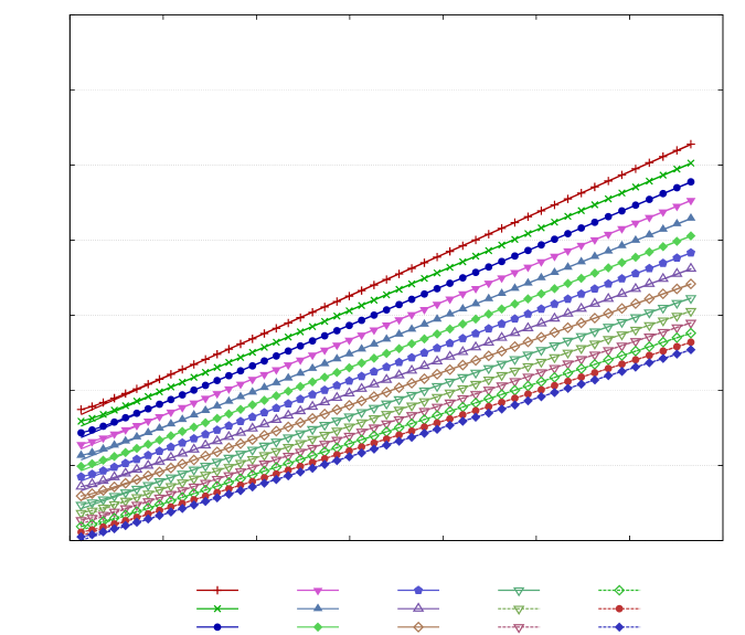
0.200.20-0.200.000.000.000.200.200.200.400.400.400.600.600.600.800.800.801.001.001.001.201.201.200.000.000.000.100.100.100.200.200.200.300.300.300.400.400.400.500.500.500.600.600.600.700.700.70

zLWsubscript𝑧𝐿𝑊z_{\scriptscriptstyle LW}

zFLRWsubscript𝑧𝐹𝐿𝑅𝑊z_{\scriptscriptstyle FLRW}zLW= 1.0994zFLRW+ 0.1225,subscript𝑧𝐿𝑊1.0994subscript𝑧𝐹𝐿𝑅𝑊0.1225z_{\scriptscriptstyle LW}\,=\,1.0994\,z_{\scriptscriptstyle FLRW}\,+\,0.1225,RMS of residuals= 7.493×10⁴RMS of residuals7.493superscript104\text{RMS of residuals}\,=\,7.493\times 10^{-4}zLW= 1.0696zFLRW+ 0.0920,subscript𝑧𝐿𝑊1.0696subscript𝑧𝐹𝐿𝑅𝑊0.0920z_{\scriptscriptstyle LW}\,=\,1.0696\,z_{\scriptscriptstyle FLRW}\,+\,0.0920,RMS of residuals= 7.290×10⁴RMS of residuals7.290superscript104\text{RMS of residuals}\,=\,7.290\times 10^{-4}zLW= 1.0400zFLRW+ 0.0618,subscript𝑧𝐿𝑊1.0400subscript𝑧𝐹𝐿𝑅𝑊0.0618z_{\scriptscriptstyle LW}\,=\,1.0400\,z_{\scriptscriptstyle FLRW}\,+\,0.0618,RMS of residuals= 7.088×10⁴RMS of residuals7.088superscript104\text{RMS of residuals}\,=\,7.088\times 10^{-4}zLW= 1.0108zFLRW+ 0.0321,subscript𝑧𝐿𝑊1.0108subscript𝑧𝐹𝐿𝑅𝑊0.0321z_{\scriptscriptstyle LW}\,=\,1.0108\,z_{\scriptscriptstyle FLRW}\,+\,0.0321,RMS of residuals= 6.890×10⁴RMS of residuals6.890superscript104\text{RMS of residuals}\,=\,6.890\times 10^{-4}zLW= 0.9823zFLRW+ 0.0030,subscript𝑧𝐿𝑊0.9823subscript𝑧𝐹𝐿𝑅𝑊0.0030z_{\scriptscriptstyle LW}\,=\,0.9823\,z_{\scriptscriptstyle FLRW}\,+\,0.0030,RMS of residuals= 6.695×10⁴RMS of residuals6.695superscript104\text{RMS of residuals}\,=\,6.695\times 10^{-4}zLW= 0.9547zFLRW 0.0253,subscript𝑧𝐿𝑊0.9547subscript𝑧𝐹𝐿𝑅𝑊0.0253z_{\scriptscriptstyle LW}\,=\,0.9547\,z_{\scriptscriptstyle FLRW}\,-\,0.0253,RMS of residuals= 6.507×10⁴RMS of residuals6.507superscript104\text{RMS of residuals}\,=\,6.507\times 10^{-4}zLW= 0.9281zFLRW 0.0524,subscript𝑧𝐿𝑊0.9281subscript𝑧𝐹𝐿𝑅𝑊0.0524z_{\scriptscriptstyle LW}\,=\,0.9281\,z_{\scriptscriptstyle FLRW}\,-\,0.0524,RMS of residuals= 6.326×10⁴RMS of residuals6.326superscript104\text{RMS of residuals}\,=\,6.326\times 10^{-4}zLW= 0.9028zFLRW 0.0783,subscript𝑧𝐿𝑊0.9028subscript𝑧𝐹𝐿𝑅𝑊0.0783z_{\scriptscriptstyle LW}\,=\,0.9028\,z_{\scriptscriptstyle FLRW}\,-\,0.0783,RMS of residuals= 6.153×10⁴RMS of residuals6.153superscript104\text{RMS of residuals}\,=\,6.153\times 10^{-4}zLW= 0.8789zFLRW 0.1026,subscript𝑧𝐿𝑊0.8789subscript𝑧𝐹𝐿𝑅𝑊0.1026z_{\scriptscriptstyle LW}\,=\,0.8789\,z_{\scriptscriptstyle FLRW}\,-\,0.1026,RMS of residuals= 5.991×10⁴RMS of residuals5.991superscript104\text{RMS of residuals}\,=\,5.991\times 10^{-4}zLW= 0.8567zFLRW 0.1253,subscript𝑧𝐿𝑊0.8567subscript𝑧𝐹𝐿𝑅𝑊0.1253z_{\scriptscriptstyle LW}\,=\,0.8567\,z_{\scriptscriptstyle FLRW}\,-\,0.1253,RMS of residuals= 5.839×10⁴RMS of residuals5.839superscript104\text{RMS of residuals}\,=\,5.839\times 10^{-4}zLW= 0.8362zFLRW 0.1462,subscript𝑧𝐿𝑊0.8362subscript𝑧𝐹𝐿𝑅𝑊0.1462z_{\scriptscriptstyle LW}\,=\,0.8362\,z_{\scriptscriptstyle FLRW}\,-\,0.1462,RMS of residuals= 5.700×10⁴RMS of residuals5.700superscript104\text{RMS of residuals}\,=\,5.700\times 10^{-4}zLW= 0.8177zFLRW 0.1651,subscript𝑧𝐿𝑊0.8177subscript𝑧𝐹𝐿𝑅𝑊0.1651z_{\scriptscriptstyle LW}\,=\,0.8177\,z_{\scriptscriptstyle FLRW}\,-\,0.1651,RMS of residuals= 5.574×10⁴RMS of residuals5.574superscript104\text{RMS of residuals}\,=\,5.574\times 10^{-4}zLW= 0.8012zFLRW 0.1819,subscript𝑧𝐿𝑊0.8012subscript𝑧𝐹𝐿𝑅𝑊0.1819z_{\scriptscriptstyle LW}\,=\,0.8012\,z_{\scriptscriptstyle FLRW}\,-\,0.1819,RMS of residuals= 5.462×10⁴RMS of residuals5.462superscript104\text{RMS of residuals}\,=\,5.462\times 10^{-4}zLW= 0.7870zFLRW 0.1964,subscript𝑧𝐿𝑊0.7870subscript𝑧𝐹𝐿𝑅𝑊0.1964z_{\scriptscriptstyle LW}\,=\,0.7870\,z_{\scriptscriptstyle FLRW}\,-\,0.1964,RMS of residuals= 5.365×10⁴RMS of residuals5.365superscript104\text{RMS of residuals}\,=\,5.365\times 10^{-4}zLW= 0.7750zFLRW 0.2086,subscript𝑧𝐿𝑊0.7750subscript𝑧𝐹𝐿𝑅𝑊0.2086z_{\scriptscriptstyle LW}\,=\,0.7750\,z_{\scriptscriptstyle FLRW}\,-\,0.2086,RMS of residuals= 5.285×10⁴RMS of residuals5.285superscript104\text{RMS of residuals}\,=\,5.285\times 10^{-4}Refer to caption1.57081.57081.57081.48491.48491.48491.39911.39911.39911.31321.31321.31321.22731.22731.22731.14141.14141.14141.05561.05561.05560.96970.96970.96970.88380.88380.88380.79800.79800.79800.71210.71210.71210.62620.62620.62620.54040.54040.54040.45450.45450.45450.36860.36860.3686
Figure 13: A plot of zLWsubscript𝑧𝐿𝑊z_{\scriptscriptstyle LW} against zFLRWsubscript𝑧𝐹𝐿𝑅𝑊z_{\scriptscriptstyle FLRW} for 15 trajectories in a flat universe with an initial cell size of rb0=3×10⁴Rsubscript𝑟subscript𝑏03superscript104𝑅r_{b_{0}}=3\times 10^{4}\,R. The initial angle θnsubscript𝜃𝑛\theta_{n} of the trajectory is given in the legend. Each trajectory was traced across 50 cells. A linear regression has been performed for each graph, with the first five data points excluded so as to focus only on the linear regime. The regression equations and corresponding root-mean-squares of the residuals are listed above in order of decreasing θnsubscript𝜃𝑛\theta_{n}.

We have simulated the propagation of photons through multiple Schwarzschild-cells for closed, flat, and open LW universes. Each time, a photon was propagated outwards in various directions from an initial radius of 10R10𝑅10\,R, R𝑅R being the Schwarzschild radius. The initial direction of travel was given, in terms of block co-ordinates, by

ka=(1,cosθn,sinθn),superscript𝑘𝑎1subscript𝜃𝑛subscript𝜃𝑛k^{a}=(1,\,\cos\theta_{n},\,\sin\theta_{n}),

with the range of θnsubscript𝜃𝑛\theta_{n} starting from the purely tangential direction of θ0=π/2subscript𝜃0𝜋2\theta_{0}=\pi/2 and decreasing until the direction was almost completely radial. Both LW and FLRW redshift factors were computed whenever the photon, while travelling outwards again, passed an observer co-moving with the source.

We can in principle re-scale the initial 𝐤𝐤\mathbf{k} by a constant factor λ𝜆\lambda, but this should not affect the redshifts: such a re-scaling would not alter the corresponding null geodesic, so the space-time points at which the observer and photon meet would remain unchanged; at these points, the only change in the photon’s frequencies would be a re-scaling by λ𝜆\lambda, but this factor would then cancel out of the redshifts. We verified this invariance of the redshifts by simulating a photon with different scalings of 𝐤𝐤\mathbf{k}, and the results, not shown, were indeed invariant for at least 11 significant figures; any discrepancies can be attributed to numerical error.

All length-scales in our simulations have been specified in terms of R𝑅R. By simply re-scaling R𝑅R in one set of results, we can readily obtain the results for an equivalent simulation where the only difference is the magnitude of R𝑅R. In particular, because redshifts are dimensionless quantities, they would not depend on the choice of R𝑅R, so we therefore made the arbitrary choice of setting R=1𝑅1R=1 for all our simulations.

0.200.20-0.200.100.10-0.100.000.000.000.100.100.100.200.200.200.300.300.300.400.400.4000200020002000400040004000600060006000800080008000100001000010000120001200012000140001400014000

z𝑧z

robs/Rsubscript𝑟𝑜𝑏𝑠𝑅r_{obs}/RRefer to captionzFLRW for θ0=12πsubscript𝑧𝐹𝐿𝑅𝑊 for subscript𝜃012𝜋z_{\scriptscriptstyle FLRW}\text{ for }\theta_{0}=\frac{1}{2}\pizLW for θ0=12πsubscript𝑧𝐿𝑊 for subscript𝜃012𝜋z_{\scriptscriptstyle LW}\text{ for }\theta_{0}=\frac{1}{2}\pizFLRW for θ29=3113000πsubscript𝑧𝐹𝐿𝑅𝑊 for subscript𝜃293113000𝜋z_{\scriptscriptstyle FLRW}\text{ for }\theta_{29}=\frac{311}{3000}\pizLW for θ29=3113000πsubscript𝑧𝐿𝑊 for subscript𝜃293113000𝜋z_{\scriptscriptstyle LW}\text{ for }\theta_{29}=\frac{311}{3000}\pi
Figure 14: A plot of redshifts z𝑧z against the radius of observation robssubscript𝑟𝑜𝑏𝑠r_{obs} for photons travelling in the flat universe with an initial cell size of rb0=3×10⁴Rsubscript𝑟subscript𝑏03superscript104𝑅r_{b_{0}}=3\times 10^{4}\,R. The photons were travelling initially in the directions of θ0=π/2subscript𝜃0𝜋2\theta_{0}=\pi/2 and θ29=311π/3000subscript𝜃29311𝜋3000\theta_{29}=311\pi/3000. Plots for both LW and FLRW redshifts are shown. All four series start at the same data point, and there is a clear jump in the LW graphs between the first and second data points.
0.000.000.000.020.020.020.040.040.040.060.060.060.080.080.080.100.100.100.120.120.120.140.140.140.160.160.160.180.180.18200020002000400040004000600060006000800080008000100001000010000120001200012000140001400014000Refer to caption

z𝑧z

robs/Rsubscript𝑟𝑜𝑏𝑠𝑅r_{obs}/RzFLRWsubscript𝑧𝐹𝐿𝑅𝑊z_{\scriptscriptstyle FLRW}zLWsubscript𝑧𝐿𝑊z_{\scriptscriptstyle LW}
Figure 15: A plot of redshifts z𝑧z against the radius of observation robssubscript𝑟𝑜𝑏𝑠r_{obs} for a photon starting instead with a position and trajectory corresponding to the second data point of the θ0=π/2subscript𝜃0𝜋2\theta_{0}=\pi/2 trajectory in Fig. 14. Plots for both LW and FLRW redshifts are shown. This time, both graphs extend smoothly out from the zero-redshift data point.
0.750.750.750.800.800.800.850.850.850.900.900.900.950.950.951.001.001.001.051.051.051.101.101.10101010100100100100010001000100001000010000100000100000100000Refer to caption

νLWsubscript𝜈𝐿𝑊\nu_{\scriptscriptstyle LW}

robs/Rsubscript𝑟𝑜𝑏𝑠𝑅r_{obs}/Rcell 1 (Eph=0.9subscript𝐸𝑝0.9E_{ph}=0.9), numericalcell 1 (Eph=0.9subscript𝐸𝑝0.9E_{ph}=0.9), analyticcell 2 (Eph=0.8795subscript𝐸𝑝0.8795E_{ph}=0.8795), analyticcell 3 (Eph=0.8596subscript𝐸𝑝0.8596E_{ph}=0.8596), analyticcell 4 (Eph=0.8403subscript𝐸𝑝0.8403E_{ph}=0.8403), analyticcell 5 (Eph=0.8214subscript𝐸𝑝0.8214E_{ph}=0.8214), analyticcell 6 (Eph=0.8032subscript𝐸𝑝0.8032E_{ph}=0.8032), analyticcell 7 (Eph=0.7854subscript𝐸𝑝0.7854E_{ph}=0.7854), analytic
Figure 16: A plot of photon frequencies νLWsubscript𝜈𝐿𝑊\nu_{\scriptscriptstyle LW} against the radius of observation robssubscript𝑟𝑜𝑏𝑠r_{obs} for a photon travelling initially in the direction of θ0=π/2subscript𝜃0𝜋2\theta_{0}=\pi/2; the initial cell size is rb0=3×10⁴Rsubscript𝑟subscript𝑏03superscript104𝑅r_{b_{0}}=3\times 10^{4}\,R. Each graph represents the photon’s frequencies within a single cell; these are the frequencies that would be seen by a co-moving observer if the photon intercepted the observer at robssubscript𝑟𝑜𝑏𝑠r_{obs}. The analytic frequencies are given by (56), and graphs for the first seven cells traversed are shown. Frequencies were also computed numerically by simulating the propagation of a photon across the first cell only; the corresponding graph is shown and completely overlaps with its analytic counterpart.
0.650.650.650.700.700.700.750.750.750.800.800.800.850.850.850.900.900.900.950.950.95101010100100100100010001000100001000010000100000100000100000Refer to caption

νLWsubscript𝜈𝐿𝑊\nu_{\scriptscriptstyle LW}

robs/Rsubscript𝑟𝑜𝑏𝑠𝑅r_{obs}/Rcell 1 (Eph=0.9subscript𝐸𝑝0.9E_{ph}=0.9), numericalcell 1 (Eph=0.9subscript𝐸𝑝0.9E_{ph}=0.9), analyticcell 2 (Eph=0.8795subscript𝐸𝑝0.8795E_{ph}=0.8795), analyticcell 3 (Eph=0.8596subscript𝐸𝑝0.8596E_{ph}=0.8596), analyticcell 4 (Eph=0.8403subscript𝐸𝑝0.8403E_{ph}=0.8403), analyticcell 5 (Eph=0.8214subscript𝐸𝑝0.8214E_{ph}=0.8214), analyticcell 6 (Eph=0.8032subscript𝐸𝑝0.8032E_{ph}=0.8032), analyticcell 7 (Eph=0.7854subscript𝐸𝑝0.7854E_{ph}=0.7854), analytic
Figure 17: The equivalent plot to Fig. 16 but for a photon travelling initially in the direction of θ29=311π/3000subscript𝜃29311𝜋3000\theta_{29}=311\pi/3000. Once again, the numerical and analytic graphs for cell 1 overlap completely.
0.000.000.000.050.050.050.100.100.100.150.150.150.200.200.200.250.250.250.300.300.300.350.350.35101010100100100100010001000100001000010000100000100000100000Refer to caption

zLWsubscript𝑧𝐿𝑊z_{\scriptscriptstyle LW}

robs/Rsubscript𝑟𝑜𝑏𝑠𝑅r_{obs}/Rcell 1 (Eph=0.9subscript𝐸𝑝0.9E_{ph}=0.9), numericalcell 1 (Eph=0.9subscript𝐸𝑝0.9E_{ph}=0.9), analytic
Figure 18: The equivalent plot to Fig. 16 but showing the redshifts zLWsubscript𝑧𝐿𝑊z_{\scriptscriptstyle LW} of cell 1 only against the radius of observation robssubscript𝑟𝑜𝑏𝑠r_{obs}. The two graphs overlap each other completely.

We have chosen the dimensions of our Regge block as follows. The angular length 2ψi2subscript𝜓𝑖2\psi_{i} was chosen so that Δϕ=2π/(3×1010)Δitalic-ϕ2𝜋3superscript1010\Delta\phi=2\pi/(3\times 10^{10}). For the closed universe, the radial length 2di2subscript𝑑𝑖2d_{i} was chosen to represent a fixed interval of Δr=107RΔ𝑟superscript107𝑅\Delta r=10^{-7}\,R. For the flat and open universes, it was instead chosen to lengthen for blocks further away from the cell centre. This lengthening was implemented so as to increase computation speed with only a marginal expense to the accuracy: the underlying continuum Schwarzschild space-time becomes flatter as one moves further away from the centre, so a flat Regge block would approximate the region more accurately. Our exact method for determining the block’s length has been described in Appendix C. Although ΔrΔ𝑟\Delta r is no longer constant, it is constrained to be an integral multiple of a minimum interval Δr0Δsubscript𝑟0\Delta r_{0}, a parameter we can freely specify, and the Regge grid is fixed so that its first set of blocks covers the region between R+Δr0𝑅Δsubscript𝑟0R+\Delta r_{0} and R+2Δr0𝑅2Δsubscript𝑟0R+2\Delta r_{0}.101010As an informal check on the accuracy, we simulated photons propagating across 100 cells in the flat, E=1𝐸1E=1 universe using both fixed and increasing block-lengths. The specific simulation parameters were an initial Schwarzschild-cell radius of rb0=3×10⁴Rsubscript𝑟subscript𝑏03superscript104𝑅r_{b_{0}}=3\times 10^{4}\,R with an initial photon radius of 10R10𝑅10R; the Regge blocks’ non-radial dimensions were Δt=10ΔrΔ𝑡10Δ𝑟\Delta t=10\,\Delta r and Δϕ=2π/(3×107)Δitalic-ϕ2𝜋3superscript107\Delta\phi=2\pi/(3\times 10^{7}); the radial dimension ΔrΔ𝑟\Delta r was fixed at 104Rsuperscript104𝑅10^{-4}R for the fixed-length simulation and was set to be at least that length for the increasing-length simulation. The two simulations’ redshift results, not shown, agreed for at least five significant figures, even at the largest radii; however the fixed block-length simulation required about 6.5 hours of computation time, while the increasing block-length simulation required only 20 minutes. As we shall see below, Δr0Δsubscript𝑟0\Delta r_{0} was chosen according to which universe was being simulated. Finally, the temporal interval was chosen to be Δt=10Δr0Δ𝑡10Δsubscript𝑟0\Delta t=10\,\Delta r_{0} for the flat and open universes and simply Δt=10ΔrΔ𝑡10Δ𝑟\Delta t=10\,\Delta r for the closed universe.

In this section we shall present the redshift results of our simulations. We begin with the flat universe, for which E=1𝐸1E=1. To investigate the effect of the initial cell size rb0subscript𝑟subscript𝑏0r_{b_{0}} on the redshifts, we have simulated flat universes for a range of initial sizes from rb0=3×10⁴Rsubscript𝑟subscript𝑏03superscript104𝑅r_{b_{0}}=3\times 10^{4}\,R to rb0=108Rsubscript𝑟subscript𝑏0superscript108𝑅r_{b_{0}}=10^{8}\,R. Following the example of Clifton and Ferreira, we have chosen the largest initial size to approximate cells with Milky Way-like masses at their centres, as this is thought to best represent our actual universe. Depending on the initial cell size, Δr0Δsubscript𝑟0\Delta r_{0} ranged from Δr0=105RΔsubscript𝑟0superscript105𝑅\Delta r_{0}=10^{-5}\,R for rb0=3×10⁴Rsubscript𝑟subscript𝑏03superscript104𝑅r_{b_{0}}=3\times 10^{4}\,R to Δr0=103RΔsubscript𝑟0superscript103𝑅\Delta r_{0}=10^{-3}\,R for rb0=108Rsubscript𝑟subscript𝑏0superscript108𝑅r_{b_{0}}=10^{8}\,R.

Figure 13 plots zLWsubscript𝑧𝐿𝑊z_{\scriptscriptstyle LW} against zFLRWsubscript𝑧𝐹𝐿𝑅𝑊z_{\scriptscriptstyle FLRW} for the universe where rb0=3×10⁴Rsubscript𝑟subscript𝑏03superscript104𝑅r_{b_{0}}=3\times 10^{4}\,R. Each trajectory was traced across 50 cells; only results for 15 trajectories are shown, although we simulated trajectories for 30 angles θnsubscript𝜃𝑛\theta_{n} ranging from θ0=π/2subscript𝜃0𝜋2\theta_{0}=\pi/2 to θ29=311π/3000subscript𝜃29311𝜋3000\theta_{29}=311\pi/3000 in decrements of 41π/300041𝜋300041\pi/3000. Apart from a brief curve at the start, each graph clearly demonstrates a strong linear relationship between zLWsubscript𝑧𝐿𝑊z_{\scriptscriptstyle LW} and zFLRWsubscript𝑧𝐹𝐿𝑅𝑊z_{\scriptscriptstyle FLRW}, and the gradient of the line is different for each angle. There are several differences, however, between our results and those of Clifton and Ferreira. Clifton and Ferreira’s graphs showed more initial scatter, which varied depending on the trajectory’s initial angle, but their graphs would eventually converge upon a common mean graph as the photon passed through an increasing number of cells. Our graphs do not display such scatter nor any common mean. However, their common mean agreed rather closely with FLRW redshifts, as it was given by 1+zLW(1+zFLRW)0.981subscript𝑧𝐿𝑊superscript1subscript𝑧𝐹𝐿𝑅𝑊0.981+z_{\scriptscriptstyle LW}\approx(1+z_{\scriptscriptstyle FLRW})^{0.98} (Clifton et al., 2012b); thus in their model, zLWsubscript𝑧𝐿𝑊z_{\scriptscriptstyle LW} and zFLRWsubscript𝑧𝐹𝐿𝑅𝑊z_{\scriptscriptstyle FLRW} are almost completely linear. Our graphs, apart from the initial curve, are completely linear, but the gradients depend on the trajectory followed.

However Clifton and Ferreira’s relation has the desirable feature of passing through the origin, since there must be zero redshift at the start of any trajectory; that is, both zLWsubscript𝑧𝐿𝑊z_{\scriptscriptstyle LW} and zFLRWsubscript𝑧𝐹𝐿𝑅𝑊z_{\scriptscriptstyle FLRW} must be zero. All our graphs instead show a jump between the origin and the next data point, and this was true of our simulations of all other universes as well. When we plotted the redshifts against the radius of observation for the rb0=3×10⁴Rsubscript𝑟subscript𝑏03superscript104𝑅r_{b_{0}}=3\times 10^{4}\,R flat universe, as shown in Fig. 14, we found that the zFLRWsubscript𝑧𝐹𝐿𝑅𝑊z_{\scriptscriptstyle FLRW} graph would extend naturally outwards from the zero-redshift point at the starting radius of 10R10𝑅10\,R, but that the zLWsubscript𝑧𝐿𝑊z_{\scriptscriptstyle LW} graph would jump suddenly from the zero-redshift point to the next data point. Suppose we ignored our current zero-redshift data point and assumed the photon actually began its trajectory at the next data point; then when we re-calculated all subsequent redshifts based on our new initial frequency for the photon, we found that the resulting zLWsubscript𝑧𝐿𝑊z_{\scriptscriptstyle LW} graph progresses naturally from the new zero-redshift point to the next data point without any jumps, as shown in Fig. 15.111111We did check this result by simulating a photon starting at the same radius and direction as that of the original photon when it generated the second data point; the resulting graph was indeed identical to that of Fig. 15.

To investigate this initial jump further, we note that in universes using CF co-ordinates, the frequency νLWsubscript𝜈𝐿𝑊\nu_{\scriptscriptstyle LW} measured by a co-moving observer can be expressed as a function of the radius at which the measurement is made, that is, the radius robssubscript𝑟𝑜𝑏𝑠r_{obs} at which the photon and observer intercept. This implies the redshifts zLWsubscript𝑧𝐿𝑊z_{\scriptscriptstyle LW} can be expressed as a function of robssubscript𝑟𝑜𝑏𝑠r_{obs}. Recall that the 4-velocity of a co-moving observer is given by (49) in Regge Schwarzschild space-time, with E=Eb𝐸subscript𝐸𝑏E=E_{b} and J=0𝐽0J=0; this vector is a function of the observer’s radial position alone. The 4-momentum of the photon is given by the same relation as well but with E=Eph𝐸subscript𝐸𝑝E=E_{ph} and J𝐽J an arbitrary constant; as long as the photon does not cross into the next cell, Ephsubscript𝐸𝑝E_{ph} will be constant, so this vector is also a function of the photon’s radial position alone. When the observer and photon intercept, they will have the same radial position, that is, the same value for r𝑟r, and we have denoted above this common r𝑟r by robssubscript𝑟𝑜𝑏𝑠r_{obs}. By taking the scalar product of these two vectors, we obtain the measured frequency as a function depending only on the value of robssubscript𝑟𝑜𝑏𝑠r_{obs},

νLW=EbEph12mrobs[(Eb12mrobs1)(Eph12mrobsJ2robs2)]1/2.subscript𝜈𝐿𝑊subscript𝐸𝑏subscript𝐸𝑝12𝑚subscript𝑟𝑜𝑏𝑠superscriptdelimited-[]subscript𝐸𝑏12𝑚subscript𝑟𝑜𝑏𝑠1subscript𝐸𝑝12𝑚subscript𝑟𝑜𝑏𝑠superscript𝐽2subscriptsuperscript𝑟2𝑜𝑏𝑠12\begin{split}\nu_{\scriptscriptstyle LW}={}&\frac{\sqrt{E_{b}\,E_{ph}}}{1-\frac{2m}{r_{obs}}}\\ &{}-\left[\left(\frac{E_{b}}{1-\frac{2m}{r_{obs}}}-1\right)\left(\frac{E_{ph}}{1-\frac{2m}{r_{obs}}}-\frac{J^{2}}{r^{2}_{obs}}\right)\right]^{1/2}.\end{split} (56)

We note that if the photon were to cross into the next cell, this relation would still hold, but from the boundary conditions, Ephsubscript𝐸𝑝E_{ph} only would change.121212Although we have an analytic function for zLWsubscript𝑧𝐿𝑊z_{\scriptscriptstyle LW} based on robssubscript𝑟𝑜𝑏𝑠r_{obs}, we must rely on the simulation to tell us where robssubscript𝑟𝑜𝑏𝑠r_{obs} is, that is, where the photon intercepts the observer. And although we can also determine Ephsubscript𝐸𝑝E_{ph} analytically from the boundary condition, to do this, we still need to know the radius at which the photon and cell boundary intercept, and we must rely on the simulation to tell us this radius as well. In Fig. 16 and Fig. 17, we have plotted this function for photons travelling at initial angles of π/2𝜋2\pi/2 and 311π/3000311𝜋3000311\pi/3000, respectively, in the rb0=3×10⁴Rsubscript𝑟subscript𝑏03superscript104𝑅r_{b_{0}}=3\times 10^{4}\,R flat universe. We have included plots for different Ephsubscript𝐸𝑝E_{ph} corresponding to the first few cells traversed. We have also simulated a photon’s propagation across the first cell for both trajectories, and for a selection of radii, we have computed the frequencies that a co-moving observer would measure if at those radii. These numerical results are also included in the figures, and we see that they agree very closely with their analytic counterparts. In Fig. 18, we show redshifts zLWsubscript𝑧𝐿𝑊z_{\scriptscriptstyle LW} instead against robssubscript𝑟𝑜𝑏𝑠r_{obs} for the θ0=π/2subscript𝜃0𝜋2\theta_{0}=\pi/2 photon travelling through cell 1 only.
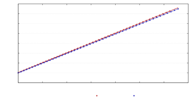
0.10.1-0.10.00.00.00.10.10.10.20.20.20.30.30.30.40.40.40.50.50.50.60.60.60.70.70.70.00.00.00.10.10.10.20.20.20.30.30.30.40.40.40.50.50.50.60.60.60.70.70.7zLW= 0.9973zFLRW+ 0.0048subscript𝑧𝐿𝑊0.9973subscript𝑧𝐹𝐿𝑅𝑊0.0048z_{\scriptscriptstyle LW}\,=\,0.9973\,z_{\scriptscriptstyle FLRW}\,+\,0.0048,RMS of residuals= 1.84×10⁵RMS of residuals1.84superscript105\text{RMS of residuals}\,=\,1.84\times 10^{-5}zLW= 0.9884zFLRW 0.0017subscript𝑧𝐿𝑊0.9884subscript𝑧𝐹𝐿𝑅𝑊0.0017z_{\scriptscriptstyle LW}\,=\,0.9884\,z_{\scriptscriptstyle FLRW}\,-\,0.0017,RMS of residuals= 7.94×10⁵RMS of residuals7.94superscript105\text{RMS of residuals}\,=\,7.94\times 10^{-5}Refer to caption

zLWsubscript𝑧𝐿𝑊z_{\scriptscriptstyle LW}

zFLRWsubscript𝑧𝐹𝐿𝑅𝑊z_{\scriptscriptstyle FLRW}1.57081.57081.57080.36860.36860.3686
(a)
0.0100.010-0.0100.0080.008-0.0080.0060.006-0.0060.0040.004-0.0040.0020.002-0.0020.0000.0000.0000.0020.0020.0020.0040.0040.0040.0060.0060.0060.000.000.000.100.100.100.200.200.200.300.300.300.400.400.400.500.500.500.600.600.600.700.700.70Refer to caption

zLWzFLRWsubscript𝑧𝐿𝑊subscript𝑧𝐹𝐿𝑅𝑊z_{\scriptscriptstyle LW}-z_{\scriptscriptstyle FLRW}

zFLRWsubscript𝑧𝐹𝐿𝑅𝑊z_{\scriptscriptstyle FLRW}1.57081.57081.57081.48491.48491.48491.39911.39911.39911.31321.31321.31321.22731.22731.22731.14141.14141.14141.05561.05561.05560.96970.96970.96970.88380.88380.88380.79800.79800.79800.71210.71210.71210.62620.62620.62620.54040.54040.54040.45450.45450.45450.36860.36860.3686
(b)
Figure 19: (a) A plot of zLWsubscript𝑧𝐿𝑊z_{\scriptscriptstyle LW} against zFLRWsubscript𝑧𝐹𝐿𝑅𝑊z_{\scriptscriptstyle FLRW} for a tangential and a nearly radial trajectory in the flat universe with initial cell size of rb0=3×10⁴Rsubscript𝑟subscript𝑏03superscript104𝑅r_{b_{0}}=3\times 10^{4}\,R. This is the equivalent plot to that of Fig. 13 but with the photon starting at 104Rsuperscript104𝑅10^{4}\,R instead. The regression lines now pass very close to the origin, and the initial curve is nearly absent; we also note that the gradients are nearly unity. Other trajectories, not shown, showed similar behaviour. (b) A plot of zLWzFLRWsubscript𝑧𝐿𝑊subscript𝑧𝐹𝐿𝑅𝑊z_{\scriptscriptstyle LW}-z_{\scriptscriptstyle FLRW} against zFLRWsubscript𝑧𝐹𝐿𝑅𝑊z_{\scriptscriptstyle FLRW} for 15 trajectories in the same universe, including the two trajectories in (a). Each graph still shows an initial curve, but it is small and short-lived, and linearity is soon established.
Table 1: Linear regression equations and the root-mean-squares of the corresponding residuals for zLWsubscript𝑧𝐿𝑊z_{\scriptscriptstyle LW} versus zFLRWsubscript𝑧𝐹𝐿𝑅𝑊z_{\scriptscriptstyle FLRW} graphs from simulations of photons in the flat universe. The initial cell size was rb0=3×10⁴Rsubscript𝑟subscript𝑏03superscript104𝑅r_{b_{0}}=3\times 10^{4}\,R. This is the same simulation as for Fig. 19. The constants in the regression equations here are much smaller than those in the regression equations in Fig. 13.
Initial angle Regression equation RMS of residuals
1.5708 zLW= 0.9973zFLRW+ 4.75×10³subscript𝑧𝐿𝑊0.9973subscript𝑧𝐹𝐿𝑅𝑊4.75superscript103z_{\scriptscriptstyle LW}\,=\,0.9973\,z_{\scriptscriptstyle FLRW}\,+\,4.75\times 10^{-3} 1.84×1051.84superscript1051.84\times 10^{-5}
1.4849 zLW= 0.9966zFLRW+ 4.07×10³subscript𝑧𝐿𝑊0.9966subscript𝑧𝐹𝐿𝑅𝑊4.07superscript103z_{\scriptscriptstyle LW}\,=\,0.9966\,z_{\scriptscriptstyle FLRW}\,+\,4.07\times 10^{-3} 1.88×1051.88superscript1051.88\times 10^{-5}
1.3991 zLW= 0.9959zFLRW+ 3.41×10³subscript𝑧𝐿𝑊0.9959subscript𝑧𝐹𝐿𝑅𝑊3.41superscript103z_{\scriptscriptstyle LW}\,=\,0.9959\,z_{\scriptscriptstyle FLRW}\,+\,3.41\times 10^{-3} 2.03×1052.03superscript1052.03\times 10^{-5}
1.3132 zLW= 0.9952zFLRW+ 2.78×10³subscript𝑧𝐿𝑊0.9952subscript𝑧𝐹𝐿𝑅𝑊2.78superscript103z_{\scriptscriptstyle LW}\,=\,0.9952\,z_{\scriptscriptstyle FLRW}\,+\,2.78\times 10^{-3} 2.29×1052.29superscript1052.29\times 10^{-5}
1.2273 zLW= 0.9944zFLRW+ 2.18×10³subscript𝑧𝐿𝑊0.9944subscript𝑧𝐹𝐿𝑅𝑊2.18superscript103z_{\scriptscriptstyle LW}\,=\,0.9944\,z_{\scriptscriptstyle FLRW}\,+\,2.18\times 10^{-3} 2.63×1052.63superscript1052.63\times 10^{-5}
1.1414 zLW= 0.9937zFLRW+ 1.62×10³subscript𝑧𝐿𝑊0.9937subscript𝑧𝐹𝐿𝑅𝑊1.62superscript103z_{\scriptscriptstyle LW}\,=\,0.9937\,z_{\scriptscriptstyle FLRW}\,+\,1.62\times 10^{-3} 3.05×1053.05superscript1053.05\times 10^{-5}
1.0556 zLW= 0.9929zFLRW+ 1.09×10³subscript𝑧𝐿𝑊0.9929subscript𝑧𝐹𝐿𝑅𝑊1.09superscript103z_{\scriptscriptstyle LW}\,=\,0.9929\,z_{\scriptscriptstyle FLRW}\,+\,1.09\times 10^{-3} 3.53×1053.53superscript1053.53\times 10^{-5}
0.9697 zLW= 0.9922zFLRW+ 6.06×10⁴subscript𝑧𝐿𝑊0.9922subscript𝑧𝐹𝐿𝑅𝑊6.06superscript104z_{\scriptscriptstyle LW}\,=\,0.9922\,z_{\scriptscriptstyle FLRW}\,+\,6.06\times 10^{-4} 4.04×1054.04superscript1054.04\times 10^{-5}
0.8838 zLW= 0.9915zFLRW+ 1.75×10⁴subscript𝑧𝐿𝑊0.9915subscript𝑧𝐹𝐿𝑅𝑊1.75superscript104z_{\scriptscriptstyle LW}\,=\,0.9915\,z_{\scriptscriptstyle FLRW}\,+\,1.75\times 10^{-4} 4.89×1054.89superscript1054.89\times 10^{-5}
0.7980 zLW= 0.9908zFLRW 2.35×10⁴subscript𝑧𝐿𝑊0.9908subscript𝑧𝐹𝐿𝑅𝑊2.35superscript104z_{\scriptscriptstyle LW}\,=\,0.9908\,z_{\scriptscriptstyle FLRW}\,-\,2.35\times 10^{-4} 5.49×1055.49superscript1055.49\times 10^{-5}
0.7121 zLW= 0.9902zFLRW 6.06×10⁴subscript𝑧𝐿𝑊0.9902subscript𝑧𝐹𝐿𝑅𝑊6.06superscript104z_{\scriptscriptstyle LW}\,=\,0.9902\,z_{\scriptscriptstyle FLRW}\,-\,6.06\times 10^{-4} 6.07×1056.07superscript1056.07\times 10^{-5}
0.6262 zLW= 0.9897zFLRW 9.37×10⁴subscript𝑧𝐿𝑊0.9897subscript𝑧𝐹𝐿𝑅𝑊9.37superscript104z_{\scriptscriptstyle LW}\,=\,0.9897\,z_{\scriptscriptstyle FLRW}\,-\,9.37\times 10^{-4} 6.62×1056.62superscript1056.62\times 10^{-5}
0.5404 zLW= 0.9892zFLRW 1.23×10³subscript𝑧𝐿𝑊0.9892subscript𝑧𝐹𝐿𝑅𝑊1.23superscript103z_{\scriptscriptstyle LW}\,=\,0.9892\,z_{\scriptscriptstyle FLRW}\,-\,1.23\times 10^{-3} 7.12×1057.12superscript1057.12\times 10^{-5}
0.4545 zLW= 0.9888zFLRW 1.48×10³subscript𝑧𝐿𝑊0.9888subscript𝑧𝐹𝐿𝑅𝑊1.48superscript103z_{\scriptscriptstyle LW}\,=\,0.9888\,z_{\scriptscriptstyle FLRW}\,-\,1.48\times 10^{-3} 7.57×1057.57superscript1057.57\times 10^{-5}
0.3686 zLW= 0.9884zFLRW 1.69×10³subscript𝑧𝐿𝑊0.9884subscript𝑧𝐹𝐿𝑅𝑊1.69superscript103z_{\scriptscriptstyle LW}\,=\,0.9884\,z_{\scriptscriptstyle FLRW}\,-\,1.69\times 10^{-3} 7.94×1057.94superscript1057.94\times 10^{-5}
0.130.130.130.140.140.140.150.150.150.160.160.160.170.170.170.180.180.180.190.190.190.200.200.200.210.210.210.220.220.220.230.230.230.000.000.000.020.020.020.040.040.040.060.060.060.080.080.080.100.100.10

zLWsubscript𝑧𝐿𝑊z_{\scriptscriptstyle LW}

zFLRWsubscript𝑧𝐹𝐿𝑅𝑊z_{\scriptscriptstyle FLRW}Refer to caption
(a)
0.1200.1200.1200.1250.1250.1250.1300.1300.1300.1350.1350.1350.1400.1400.1400.1450.1450.1450.1500.1500.1500.0000.0000.0000.0050.0050.0050.0100.0100.0100.0150.0150.0150.0200.0200.0200.0250.0250.0250.0300.0300.0300.0350.0350.035

zLWsubscript𝑧𝐿𝑊z_{\scriptscriptstyle LW}

zFLRWsubscript𝑧𝐹𝐿𝑅𝑊z_{\scriptscriptstyle FLRW}Refer to caption
(b)
0.1150.1150.1150.1160.1160.1160.1170.1170.1170.1180.1180.1180.1190.1190.1190.1200.1200.1200.1210.1210.1210.1220.1220.1220.1230.1230.1230.1240.1240.1240.0000.0000.0000.0020.0020.0020.0040.0040.0040.0060.0060.0060.0080.0080.0080.0100.0100.010

zLWsubscript𝑧𝐿𝑊z_{\scriptscriptstyle LW}

zFLRWsubscript𝑧𝐹𝐿𝑅𝑊z_{\scriptscriptstyle FLRW}Refer to caption
(c)
0.11250.11250.11250.11300.11300.11300.11350.11350.11350.11400.11400.11400.11450.11450.11450.11500.11500.11500.11550.11550.11550.00000.00000.00000.00050.00050.00050.00100.00100.00100.00150.00150.00150.00200.00200.00200.00250.00250.00250.00300.00300.00300.00350.00350.0035

zLWsubscript𝑧𝐿𝑊z_{\scriptscriptstyle LW}

zFLRWsubscript𝑧𝐹𝐿𝑅𝑊z_{\scriptscriptstyle FLRW}Refer to caption
(d)
Figure 20: A plot of zLWsubscript𝑧𝐿𝑊z_{\scriptscriptstyle LW} against zFLRWsubscript𝑧𝐹𝐿𝑅𝑊z_{\scriptscriptstyle FLRW} for the θ0=π/2subscript𝜃0𝜋2\theta_{0}=\pi/2 photon trajectory in the (a) rb0=105Rsubscript𝑟subscript𝑏0superscript105𝑅r_{b_{0}}=10^{5}\,R universe, (b) rb0=106Rsubscript𝑟subscript𝑏0superscript106𝑅r_{b_{0}}=10^{6}\,R universe, (c) rb0=107Rsubscript𝑟subscript𝑏0superscript107𝑅r_{b_{0}}=10^{7}\,R universe, and (d) rb0=108Rsubscript𝑟subscript𝑏0superscript108𝑅r_{b_{0}}=10^{8}\,R universe. Δr0Δsubscript𝑟0\Delta r_{0} was 105Rsuperscript105𝑅10^{-5}\,R for (a) and (b), 104Rsuperscript104𝑅10^{-4}\,R for (c), and 103Rsuperscript103𝑅10^{-3}\,R for (d).
0.00050.0005-0.00050.00000.00000.00000.00050.00050.00050.00100.00100.00100.00150.00150.00150.00200.00200.00200.00250.00250.00250.00300.00300.00300.00350.00350.00350.00000.00000.00000.00050.00050.00050.00100.00100.00100.00150.00150.00150.00200.00200.00200.00250.00250.00250.00300.00300.00300.00350.00350.0035zLW= 1.0215zFLRW+ 5.4×10⁵subscript𝑧𝐿𝑊1.0215subscript𝑧𝐹𝐿𝑅𝑊5.4superscript105z_{\scriptscriptstyle LW}\,=\,1.0215\,z_{\scriptscriptstyle FLRW}\,+\,5.4\times 10^{-5},RMS of residuals= 1.66×10⁶RMS of residuals1.66superscript106\text{RMS of residuals}\,=\,1.66\times 10^{-6}zLW= 0.9967zFLRW 1.6×10⁷subscript𝑧𝐿𝑊0.9967subscript𝑧𝐹𝐿𝑅𝑊1.6superscript107z_{\scriptscriptstyle LW}\,=\,0.9967\,z_{\scriptscriptstyle FLRW}\,-\,1.6\times 10^{-7},RMS of residuals= 1.24×10⁸RMS of residuals1.24superscript108\text{RMS of residuals}\,=\,1.24\times 10^{-8}Refer to caption

zLWsubscript𝑧𝐿𝑊z_{\scriptscriptstyle LW}

zFLRWsubscript𝑧𝐹𝐿𝑅𝑊z_{\scriptscriptstyle FLRW}1.57081.57081.57080.39010.39010.3901
(a)
2.0×1052.0superscript105-2.0\times 10^{-5}0.0×1050.0superscript1050.0\times 10^{-5}2.0×1052.0superscript1052.0\times 10^{-5}4.0×1054.0superscript1054.0\times 10^{-5}6.0×1056.0superscript1056.0\times 10^{-5}8.0×1058.0superscript1058.0\times 10^{-5}10.0×10510.0superscript10510.0\times 10^{-5}12.0×10512.0superscript10512.0\times 10^{-5}0.00000.00000.00000.00050.00050.00050.00100.00100.00100.00150.00150.00150.00200.00200.00200.00250.00250.00250.00300.00300.00300.00350.00350.0035Refer to caption

zLWzFLRWsubscript𝑧𝐿𝑊subscript𝑧𝐹𝐿𝑅𝑊z_{\scriptscriptstyle LW}-z_{\scriptscriptstyle FLRW}

zFLRWsubscript𝑧𝐹𝐿𝑅𝑊z_{\scriptscriptstyle FLRW}1.57081.57081.57081.46351.46351.46351.35611.35611.35611.24881.24881.24881.14141.14141.14141.03411.03411.03410.92680.92680.92680.81940.81940.81940.71210.71210.71210.60480.60480.60480.49740.49740.49740.39010.39010.3901
(b)
Figure 21: (a) A plot of zLWsubscript𝑧𝐿𝑊z_{\scriptscriptstyle LW} against zFLRWsubscript𝑧𝐹𝐿𝑅𝑊z_{\scriptscriptstyle FLRW} for a tangential and a nearly radial trajectory starting at radius 107Rsuperscript107𝑅10^{7}\,R in the rb0=108Rsubscript𝑟subscript𝑏0superscript108𝑅r_{b_{0}}=10^{8}\,R flat universe. Each trajectory was traced across 15 cells. Compared to Fig. 19a, the regression lines here pass even closer to the origin; the initial curve is even more suppressed; and the gradients are even closer to unity. Other trajectories, not shown, showed similar behaviour. (b) A plot of zLWzFLRWsubscript𝑧𝐿𝑊subscript𝑧𝐹𝐿𝑅𝑊z_{\scriptscriptstyle LW}-z_{\scriptscriptstyle FLRW} against zFLRWsubscript𝑧𝐹𝐿𝑅𝑊z_{\scriptscriptstyle FLRW} for 15 trajectories in the same universe, including the two trajectories in (a). Compared to Fig. 19b, the initial curve here is even smaller and more short-lived.
Table 2: Linear regression equations and the root-mean-squares of the corresponding residuals for zLWsubscript𝑧𝐿𝑊z_{\scriptscriptstyle LW} versus zFLRWsubscript𝑧𝐹𝐿𝑅𝑊z_{\scriptscriptstyle FLRW} graphs from simulations of photons in the rb0=108Rsubscript𝑟subscript𝑏0superscript108𝑅r_{b_{0}}=10^{8}\,R flat universe. This is the same simulation as for Fig. 21a and Fig. 21b. Regression was performed on the zFLRW>0.001subscript𝑧𝐹𝐿𝑅𝑊0.001z_{\scriptscriptstyle FLRW}>0.001 region. Both the regression equation constants and the residuals are even smaller here than in Table 1.
Initial angle Regression equation RMS of residuals
1.5708 zLW= 1.0215zFLRW+ 5.4×10⁵subscript𝑧𝐿𝑊1.0215subscript𝑧𝐹𝐿𝑅𝑊5.4superscript105z_{\scriptscriptstyle LW}\,=\,1.0215\,z_{\scriptscriptstyle FLRW}\,+\,5.4\times 10^{-5} 1.66×1061.66superscript1061.66\times 10^{-6}
1.4635 zLW= 1.0200zFLRW+ 2.9×10⁵subscript𝑧𝐿𝑊1.0200subscript𝑧𝐹𝐿𝑅𝑊2.9superscript105z_{\scriptscriptstyle LW}\,=\,1.0200\,z_{\scriptscriptstyle FLRW}\,+\,2.9\times 10^{-5} 1.45×1061.45superscript1061.45\times 10^{-6}
1.3561 zLW= 1.0167zFLRW+ 1.5×10⁵subscript𝑧𝐿𝑊1.0167subscript𝑧𝐹𝐿𝑅𝑊1.5superscript105z_{\scriptscriptstyle LW}\,=\,1.0167\,z_{\scriptscriptstyle FLRW}\,+\,1.5\times 10^{-5} 1.04×1061.04superscript1061.04\times 10^{-6}
1.2488 zLW= 1.0130zFLRW+ 8.8×10⁶subscript𝑧𝐿𝑊1.0130subscript𝑧𝐹𝐿𝑅𝑊8.8superscript106z_{\scriptscriptstyle LW}\,=\,1.0130\,z_{\scriptscriptstyle FLRW}\,+\,8.8\times 10^{-6} 6.97×1076.97superscript1076.97\times 10^{-7}
1.1414 zLW= 1.0095zFLRW+ 5.4×10⁶subscript𝑧𝐿𝑊1.0095subscript𝑧𝐹𝐿𝑅𝑊5.4superscript106z_{\scriptscriptstyle LW}\,=\,1.0095\,z_{\scriptscriptstyle FLRW}\,+\,5.4\times 10^{-6} 4.62×1074.62superscript1074.62\times 10^{-7}
1.0341 zLW= 1.0066zFLRW+ 3.4×10⁶subscript𝑧𝐿𝑊1.0066subscript𝑧𝐹𝐿𝑅𝑊3.4superscript106z_{\scriptscriptstyle LW}\,=\,1.0066\,z_{\scriptscriptstyle FLRW}\,+\,3.4\times 10^{-6} 3.08×1073.08superscript1073.08\times 10^{-7}
0.9268 zLW= 1.0041zFLRW+ 2.2×10⁶subscript𝑧𝐿𝑊1.0041subscript𝑧𝐹𝐿𝑅𝑊2.2superscript106z_{\scriptscriptstyle LW}\,=\,1.0041\,z_{\scriptscriptstyle FLRW}\,+\,2.2\times 10^{-6} 2.04×1072.04superscript1072.04\times 10^{-7}
0.8194 zLW= 1.0020zFLRW+ 1.4×10⁶subscript𝑧𝐿𝑊1.0020subscript𝑧𝐹𝐿𝑅𝑊1.4superscript106z_{\scriptscriptstyle LW}\,=\,1.0020\,z_{\scriptscriptstyle FLRW}\,+\,1.4\times 10^{-6} 1.31×1071.31superscript1071.31\times 10^{-7}
0.7121 zLW= 1.0002zFLRW+ 9.2×10⁷subscript𝑧𝐿𝑊1.0002subscript𝑧𝐹𝐿𝑅𝑊9.2superscript107z_{\scriptscriptstyle LW}\,=\,1.0002\,z_{\scriptscriptstyle FLRW}\,+\,9.2\times 10^{-7} 6.34×1086.34superscript1086.34\times 10^{-8}
0.6048 zLW= 0.9988zFLRW+ 4.5×10⁷subscript𝑧𝐿𝑊0.9988subscript𝑧𝐹𝐿𝑅𝑊4.5superscript107z_{\scriptscriptstyle LW}\,=\,0.9988\,z_{\scriptscriptstyle FLRW}\,+\,4.5\times 10^{-7} 3.10×1083.10superscript1083.10\times 10^{-8}
0.4974 zLW= 0.9976zFLRW+ 1.0×10⁷subscript𝑧𝐿𝑊0.9976subscript𝑧𝐹𝐿𝑅𝑊1.0superscript107z_{\scriptscriptstyle LW}\,=\,0.9976\,z_{\scriptscriptstyle FLRW}\,+\,1.0\times 10^{-7} 7.08×1097.08superscript1097.08\times 10^{-9}
0.3901 zLW= 0.9967zFLRW 1.6×10⁷subscript𝑧𝐿𝑊0.9967subscript𝑧𝐹𝐿𝑅𝑊1.6superscript107z_{\scriptscriptstyle LW}\,=\,0.9967\,z_{\scriptscriptstyle FLRW}\,-\,1.6\times 10^{-7} 1.24×1081.24superscript1081.24\times 10^{-8}
0.600.600.600.700.700.700.800.800.800.900.900.901.001.001.001.101.101.101.201.201.200.000.000.000.100.100.100.200.200.200.300.300.300.400.400.400.500.500.500.600.600.600.700.700.700.800.800.800.900.900.901.001.001.00

gradient of zLWgradient of subscript𝑧𝐿𝑊\text{gradient of }z_{\scriptscriptstyle LW}vs zFLRWsubscript𝑧𝐹𝐿𝑅𝑊z_{\scriptscriptstyle FLRW}

cos(θ)𝜃\cos(\theta)gradient=0.3477cos(θ)+ 1.0994gradient0.3477𝜃1.0994\text{gradient}\,=\,-0.3477\,\cos(\theta)\,+\,1.0994RMS of residuals= 7.01×10⁶RMS of residuals7.01superscript106\text{RMS of residuals}\,=\,7.01\times 10^{-6}gradient=0.3380cos(θ)+ 1.0689gradient0.3380𝜃1.0689\text{gradient}\,=\,-0.3380\,\cos(\theta)\,+\,1.0689RMS of residuals= 2.11×10⁶RMS of residuals2.11superscript106\text{RMS of residuals}\,=\,2.11\times 10^{-6}gradient=0.3322cos(θ)+ 1.0504gradient0.3322𝜃1.0504\text{gradient}\,=\,-0.3322\,\cos(\theta)\,+\,1.0504RMS of residuals= 2.16×10⁷RMS of residuals2.16superscript107\text{RMS of residuals}\,=\,2.16\times 10^{-7}gradient=0.3234cos(θ)+ 1.0226gradient0.3234𝜃1.0226\text{gradient}\,=\,-0.3234\,\cos(\theta)\,+\,1.0226RMS of residuals= 2.11×10⁸RMS of residuals2.11superscript108\text{RMS of residuals}\,=\,2.11\times 10^{-8}gradient=0.3104cos(θ)+ 0.9814gradient0.3104𝜃0.9814\text{gradient}\,=\,-0.3104\,\cos(\theta)\,+\,0.9814RMS of residuals= 1.99×10⁹RMS of residuals1.99superscript109\text{RMS of residuals}\,=\,1.99\times 10^{-9}Refer to captionrb=3×10⁴subscript𝑟𝑏3superscript104r_{b}=3\times 10^{4}rb=105subscript𝑟𝑏superscript105r_{b}=10^{5}rb=106subscript𝑟𝑏superscript106r_{b}=10^{6}rb=107subscript𝑟𝑏superscript107r_{b}=10^{7}rb=108subscript𝑟𝑏superscript108r_{b}=10^{8}
Figure 22: A plot of the gradients of zLWsubscript𝑧𝐿𝑊z_{\scriptscriptstyle LW} vs zFLRWsubscript𝑧𝐹𝐿𝑅𝑊z_{\scriptscriptstyle FLRW} graphs against cos(θn)subscript𝜃𝑛\cos(\theta_{n}) for flat universes of different initial cell size rb0subscript𝑟subscript𝑏0r_{b_{0}}. A linear regression has been performed on each graph, and the regression equations are displayed in order of increasing rb0subscript𝑟subscript𝑏0r_{b_{0}}.

Based on these graphs, we make some speculations on the origin of the jump as well as the initial curve in the zLWsubscript𝑧𝐿𝑊z_{\scriptscriptstyle LW} vs zFLRWsubscript𝑧𝐹𝐿𝑅𝑊z_{\scriptscriptstyle FLRW} graphs. We note that for large robssubscript𝑟𝑜𝑏𝑠r_{obs}, the frequency asymptotically approaches

νasymsubscript𝜈𝑎𝑠𝑦𝑚\displaystyle\nu_{asym} =Eph(EbEb1)absentsubscript𝐸𝑝subscript𝐸𝑏subscript𝐸𝑏1\displaystyle=\sqrt{E_{ph}}\left(\sqrt{E_{b}}-\sqrt{E_{b}-1}\right)
=Ephfor Eb=1.formulae-sequenceabsentsubscript𝐸𝑝for subscript𝐸𝑏1\displaystyle=\sqrt{E_{ph}}\qquad\text{for }E_{b}=1.

Equivalently, the redshift asymptotically approaches

zasymsubscript𝑧𝑎𝑠𝑦𝑚\displaystyle z_{asym} =νeEph(EbEb1)1absentsubscript𝜈𝑒subscript𝐸𝑝subscript𝐸𝑏subscript𝐸𝑏11\displaystyle=\frac{\nu_{e}}{\sqrt{E_{ph}}\left(\sqrt{E_{b}}-\sqrt{E_{b}-1}\right)}-1
=νeEph1for Eb=1.formulae-sequenceabsentsubscript𝜈𝑒subscript𝐸𝑝1for subscript𝐸𝑏1\displaystyle=\frac{\nu_{e}}{\sqrt{E_{ph}}}-1\qquad\text{for }E_{b}=1.

As the photon traversed ever more cells in our simulations, we found that it would intercept the co-moving observer at ever larger robssubscript𝑟𝑜𝑏𝑠r_{obs}. So after enough cells, zLWsubscript𝑧𝐿𝑊z_{\scriptscriptstyle LW} should be very close to the asymptotic value zasymsubscript𝑧𝑎𝑠𝑦𝑚z_{asym}. Also from our simulations, we found that Ephsubscript𝐸𝑝E_{ph} would decrease with each subsequent cell implying that zasymsubscript𝑧𝑎𝑠𝑦𝑚z_{asym} would increase, which is consistent with the zLWsubscript𝑧𝐿𝑊z_{\scriptscriptstyle LW} vs zFLRWsubscript𝑧𝐹𝐿𝑅𝑊z_{\scriptscriptstyle FLRW} graphs’ positive gradients. Thus the asymptotic, large-radius behaviour of the redshifts is responsible for the linear behaviour of the zLWsubscript𝑧𝐿𝑊z_{\scriptscriptstyle LW} vs zFLRWsubscript𝑧𝐹𝐿𝑅𝑊z_{\scriptscriptstyle FLRW} graphs. The graphs’ initial behaviour however must be explained by the behaviour of the redshifts at low robssubscript𝑟𝑜𝑏𝑠r_{obs}, where the photon is still sufficiently close to the central mass to feel its influence strongly. We note that the frequencies always approach νasymsubscript𝜈𝑎𝑠𝑦𝑚\nu_{asym} from below, implying that the redshifts always approach zasymsubscript𝑧𝑎𝑠𝑦𝑚z_{asym} from above. This is consistent with the initial curve in the zLWsubscript𝑧𝐿𝑊z_{\scriptscriptstyle LW} vs zFLRWsubscript𝑧𝐹𝐿𝑅𝑊z_{\scriptscriptstyle FLRW} graphs, as this curve converges into the linear regime from above as well. At much smaller robssubscript𝑟𝑜𝑏𝑠r_{obs} however, the redshift may deviate much more significantly from the asymptotic value. In particular, the deviation of the zero-redshift point, where robssubscript𝑟𝑜𝑏𝑠r_{obs} is smallest, may be much greater than the deviation of the next data point, where robssubscript𝑟𝑜𝑏𝑠r_{obs} may have increased sufficiently for the redshift to be much closer to the asymptotic value. This would account for the sudden initial jump seen in the zLWsubscript𝑧𝐿𝑊z_{\scriptscriptstyle LW} vs zFLRWsubscript𝑧𝐹𝐿𝑅𝑊z_{\scriptscriptstyle FLRW} graphs. Therefore, the initial jump and the initial curve in the zLWsubscript𝑧𝐿𝑊z_{\scriptscriptstyle LW} vs zFLRWsubscript𝑧𝐹𝐿𝑅𝑊z_{\scriptscriptstyle FLRW} graphs can be attributed to the photon being closer to the central mass and thus feeling its effects more strongly.
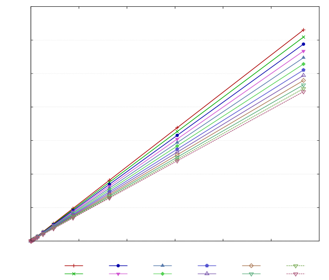
0020002000200040004000400060006000600080008000800010000100001000012000120001200014000140001400000200020002000400040004000600060006000800080008000100001000010000120001200012000

zLWsubscript𝑧𝐿𝑊z_{\scriptscriptstyle LW}

zFLRWsubscript𝑧𝐹𝐿𝑅𝑊z_{\scriptscriptstyle FLRW}zLW= 1.1109zFLRW+ 0.0908,subscript𝑧𝐿𝑊1.1109subscript𝑧𝐹𝐿𝑅𝑊0.0908z_{\scriptscriptstyle LW}\,=\,1.1109\,z_{\scriptscriptstyle FLRW}\,+\,0.0908,RMS of residuals= 0.0353RMS of residuals0.0353\text{RMS of residuals}\,=\,0.0353zLW= 1.0732zFLRW+ 0.0539,subscript𝑧𝐿𝑊1.0732subscript𝑧𝐹𝐿𝑅𝑊0.0539z_{\scriptscriptstyle LW}\,=\,1.0732\,z_{\scriptscriptstyle FLRW}\,+\,0.0539,RMS of residuals= 0.0341RMS of residuals0.0341\text{RMS of residuals}\,=\,0.0341zLW= 1.0361zFLRW+ 0.0174,subscript𝑧𝐿𝑊1.0361subscript𝑧𝐹𝐿𝑅𝑊0.0174z_{\scriptscriptstyle LW}\,=\,1.0361\,z_{\scriptscriptstyle FLRW}\,+\,0.0174,RMS of residuals= 0.0328RMS of residuals0.0328\text{RMS of residuals}\,=\,0.0328zLW= 0.9997zFLRW 0.0183,subscript𝑧𝐿𝑊0.9997subscript𝑧𝐹𝐿𝑅𝑊0.0183z_{\scriptscriptstyle LW}\,=\,0.9997\,z_{\scriptscriptstyle FLRW}\,-\,0.0183,RMS of residuals= 0.0317RMS of residuals0.0317\text{RMS of residuals}\,=\,0.0317zLW= 0.9647zFLRW 0.0526,subscript𝑧𝐿𝑊0.9647subscript𝑧𝐹𝐿𝑅𝑊0.0526z_{\scriptscriptstyle LW}\,=\,0.9647\,z_{\scriptscriptstyle FLRW}\,-\,0.0526,RMS of residuals= 0.0305RMS of residuals0.0305\text{RMS of residuals}\,=\,0.0305zLW= 0.9313zFLRW 0.0854,subscript𝑧𝐿𝑊0.9313subscript𝑧𝐹𝐿𝑅𝑊0.0854z_{\scriptscriptstyle LW}\,=\,0.9313\,z_{\scriptscriptstyle FLRW}\,-\,0.0854,RMS of residuals= 0.0294RMS of residuals0.0294\text{RMS of residuals}\,=\,0.0294zLW= 0.9000zFLRW 0.1161,subscript𝑧𝐿𝑊0.9000subscript𝑧𝐹𝐿𝑅𝑊0.1161z_{\scriptscriptstyle LW}\,=\,0.9000\,z_{\scriptscriptstyle FLRW}\,-\,0.1161,RMS of residuals= 0.0283RMS of residuals0.0283\text{RMS of residuals}\,=\,0.0283zLW= 0.8711zFLRW 0.1444,subscript𝑧𝐿𝑊0.8711subscript𝑧𝐹𝐿𝑅𝑊0.1444z_{\scriptscriptstyle LW}\,=\,0.8711\,z_{\scriptscriptstyle FLRW}\,-\,0.1444,RMS of residuals= 0.0274RMS of residuals0.0274\text{RMS of residuals}\,=\,0.0274zLW= 0.8450zFLRW 0.1700,subscript𝑧𝐿𝑊0.8450subscript𝑧𝐹𝐿𝑅𝑊0.1700z_{\scriptscriptstyle LW}\,=\,0.8450\,z_{\scriptscriptstyle FLRW}\,-\,0.1700,RMS of residuals= 0.0265RMS of residuals0.0265\text{RMS of residuals}\,=\,0.0265zLW= 0.8220zFLRW 0.1926,subscript𝑧𝐿𝑊0.8220subscript𝑧𝐹𝐿𝑅𝑊0.1926z_{\scriptscriptstyle LW}\,=\,0.8220\,z_{\scriptscriptstyle FLRW}\,-\,0.1926,RMS of residuals= 0.0257RMS of residuals0.0257\text{RMS of residuals}\,=\,0.0257zLW= 0.8022zFLRW 0.2120,subscript𝑧𝐿𝑊0.8022subscript𝑧𝐹𝐿𝑅𝑊0.2120z_{\scriptscriptstyle LW}\,=\,0.8022\,z_{\scriptscriptstyle FLRW}\,-\,0.2120,RMS of residuals= 0.0251RMS of residuals0.0251\text{RMS of residuals}\,=\,0.0251zLW= 0.7860zFLRW 0.2279,subscript𝑧𝐿𝑊0.7860subscript𝑧𝐹𝐿𝑅𝑊0.2279z_{\scriptscriptstyle LW}\,=\,0.7860\,z_{\scriptscriptstyle FLRW}\,-\,0.2279,RMS of residuals= 0.0245RMS of residuals0.0245\text{RMS of residuals}\,=\,0.0245Refer to caption1.57081.57081.57081.46351.46351.46351.35611.35611.35611.24881.24881.24881.14141.14141.14141.03411.03411.03410.92680.92680.92680.81940.81940.81940.71210.71210.71210.60480.60480.60480.49740.49740.49740.39010.39010.3901
Figure 23: A plot of zLWsubscript𝑧𝐿𝑊z_{\scriptscriptstyle LW} against zFLRWsubscript𝑧𝐹𝐿𝑅𝑊z_{\scriptscriptstyle FLRW} for 12 trajectories in the Eb=1.1subscript𝐸𝑏1.1E_{b}=1.1 universe. For this simulation, Δr0Δsubscript𝑟0\Delta r_{0} was 103Rsuperscript103𝑅10^{-3}\,R. The initial angle θnsubscript𝜃𝑛\theta_{n} of the trajectory is given in the legend. Each trajectory was traced across 15 cells. A linear regression has been performed for each graph. The regression equations and corresponding root-mean-squares of the residuals are listed above in order of decreasing θnsubscript𝜃𝑛\theta_{n}.

To test our conjecture, we simulated photons in the same universe but starting from a large radius, specifically r=104R𝑟superscript104𝑅r=10^{4}\,R, such that the central mass’ influence would be much reduced. Fig. 19a shows the resulting plot of zLWsubscript𝑧𝐿𝑊z_{\scriptscriptstyle LW} against zFLRWsubscript𝑧𝐹𝐿𝑅𝑊z_{\scriptscriptstyle FLRW} for the most radial and the most tangential trajectories simulated. The graphs now follow completely straight lines passing very close to the origin, with the initial jump completely gone and the initial curve nearly absent. All other trajectories at intermediate angles displayed similar behaviour, with the graphs’ gradients increasing as the initial trajectory became more tangential. We also note that the gradients are nearly unity, indicating that zLWsubscript𝑧𝐿𝑊z_{\scriptscriptstyle LW} is nearly identical to zFLRWsubscript𝑧𝐹𝐿𝑅𝑊z_{\scriptscriptstyle FLRW}. In Fig. 19b, we have plotted the difference between the zLWsubscript𝑧𝐿𝑊z_{\scriptscriptstyle LW} graphs and the reference graph of z~LW=zFLRWsubscript~𝑧𝐿𝑊subscript𝑧𝐹𝐿𝑅𝑊\tilde{z}_{\scriptscriptstyle LW}=z_{\scriptscriptstyle FLRW}. The deviation from linearity at low robssubscript𝑟𝑜𝑏𝑠r_{obs} becomes clearer now, although we also see that it is short-lived. From this figure, we see that linearity is relatively well established by zFLRW0.2subscript𝑧𝐹𝐿𝑅𝑊0.2z_{\scriptscriptstyle FLRW}\approx 0.2; thus for each trajectory, we have regressed the corresponding zLWsubscript𝑧𝐿𝑊z_{\scriptscriptstyle LW} vs zFLRWsubscript𝑧𝐹𝐿𝑅𝑊z_{\scriptscriptstyle FLRW} graph for the region zFLRW>0.2subscript𝑧𝐹𝐿𝑅𝑊0.2z_{\scriptscriptstyle FLRW}>0.2. All regression equations and corresponding root-mean-squares of the residuals have been listed in Table 1, and two of these regressions are shown in Fig. 19a. These equations show that our observations for the graphs in Fig. 19a holds generally for all trajectories, specifically that the gradients are nearly unity and that the graphs pass very close to the origin. Thus, the influence of the masses on redshifts has been significantly suppressed, and the redshifts now behave nearly identically to FLRW, much like Clifton and Ferreira’s mean redshift result.

For flat universes with larger initial cell sizes, our simulations yielded results similar to those of the rb0=3×10⁴Rsubscript𝑟subscript𝑏03superscript104𝑅r_{b_{0}}=3\times 10^{4}\,R universe. Figure 20 depicts plots of zLWsubscript𝑧𝐿𝑊z_{\scriptscriptstyle LW} against zFLRWsubscript𝑧𝐹𝐿𝑅𝑊z_{\scriptscriptstyle FLRW} for the θ0=π/2subscript𝜃0𝜋2\theta_{0}=\pi/2 trajectory for universes with rb0subscript𝑟subscript𝑏0r_{b_{0}} ranging from 105superscript10510^{5} to 108superscript10810^{8}. All graphs again converged quickly to a straight line from above, including graphs, not shown, for the other trajectories. One noticeable development though was that the curve at the start of the graphs became more pronounced as the initial size increased. However when we simulated photons starting from a large radius again, the initial curve was again suppressed, and the initial jump was again absent, as shown in Fig. 21a, Fig. 21b, and Table 2 for photons starting from r=107R𝑟superscript107𝑅r=10^{7}\,R in the rb0=108Rsubscript𝑟subscript𝑏0superscript108𝑅r_{b_{0}}=10^{8}\,R universe; the initial curve is even more short-lived, as seen in Fig. 21b, and the regression lines for all trajectories pass even closer to the origin, as demonstrated by the even smaller constants in the regression equations in Table 2.

We also notice, in Fig. 13, that the gradients of zLWsubscript𝑧𝐿𝑊z_{\scriptscriptstyle LW} vs zFLRWsubscript𝑧𝐹𝐿𝑅𝑊z_{\scriptscriptstyle FLRW} graphs decrease with θnsubscript𝜃𝑛\theta_{n}. In fact, if we plot the gradients against cos(θn)subscript𝜃𝑛\cos(\theta_{n}), we find a strongly linear relationship between the two quantities, as shown in Fig. 22. As the figure shows, this is also true of the gradients for all the other flat universes we simulated. Since cos(θn)subscript𝜃𝑛\cos(\theta_{n}) determines the radial component ρ˙initsubscript˙𝜌𝑖𝑛𝑖𝑡\dot{\rho}_{init} of the photon’s initial velocity, this implies that the gradients are linearly related to ρ˙init/τ˙initsubscript˙𝜌𝑖𝑛𝑖𝑡subscript˙𝜏𝑖𝑛𝑖𝑡\dot{\rho}_{init}/\dot{\tau}_{init}. As the photon’s initial velocity becomes increasingly radial, the photon’s frequency becomes increasingly blueshifted relative to the FLRW redshift. We believe this is due to the central mass’ stronger influence on the photon, as a more radial trajectory would bring the photon closer to the central mass. Quite remarkably, this influence can alter the lattice universe redshifts zLWsubscript𝑧𝐿𝑊z_{\scriptscriptstyle LW} from their FLRW counterparts zFLRWsubscript𝑧𝐹𝐿𝑅𝑊z_{\scriptscriptstyle FLRW} by as much as 30%, as shown by the right end of the rb0=108subscript𝑟subscript𝑏0superscript108r_{b_{0}}=10^{8} graph. Since the lattice universe can generate lower redshift values, an observer fitting these redshifts to an FLRW model could significantly underestimate the age of the photons’ source.
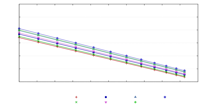
0.70.80.91.01.11.21.30.00.10.20.30.40.50.60.70.80.91.0

gradient of zLWgradient of subscript𝑧𝐿𝑊\text{gradient of }z_{\scriptscriptstyle LW}vs zFLRWsubscript𝑧𝐹𝐿𝑅𝑊z_{\scriptscriptstyle FLRW}

cos(θ)𝜃\cos(\theta)gradient=0.3291cos(θ)+ 1.0407gradient0.3291𝜃1.0407\text{gradient}\,=\,-0.3291\,\cos(\theta)\,+\,1.0407RMS of residuals= 6.57×10⁶RMS of residuals6.57superscript106\text{RMS of residuals}\,=\,6.57\times 10^{-6}gradient=0.3321cos(θ)+ 1.0499gradient0.3321𝜃1.0499\text{gradient}\,=\,-0.3321\,\cos(\theta)\,+\,1.0499RMS of residuals= 6.58×10⁶RMS of residuals6.58superscript106\text{RMS of residuals}\,=\,6.58\times 10^{-6}gradient=0.3377cos(θ)+ 1.0678gradient0.3377𝜃1.0678\text{gradient}\,=\,-0.3377\,\cos(\theta)\,+\,1.0678RMS of residuals= 6.53×10⁶RMS of residuals6.53superscript106\text{RMS of residuals}\,=\,6.53\times 10^{-6}gradient=0.3407cos(θ)+ 1.0773gradient0.3407𝜃1.0773\text{gradient}\,=\,-0.3407\,\cos(\theta)\,+\,1.0773RMS of residuals= 6.44×10⁶RMS of residuals6.44superscript106\text{RMS of residuals}\,=\,6.44\times 10^{-6}gradient=0.3463cos(θ)+ 1.0950gradient0.3463𝜃1.0950\text{gradient}\,=\,-0.3463\,\cos(\theta)\,+\,1.0950RMS of residuals= 6.03×10⁶RMS of residuals6.03superscript106\text{RMS of residuals}\,=\,6.03\times 10^{-6}gradient=0.3478cos(θ)+ 1.0999gradient0.3478𝜃1.0999\text{gradient}\,=\,-0.3478\,\cos(\theta)\,+\,1.0999RMS of residuals= 5.82×10⁶RMS of residuals5.82superscript106\text{RMS of residuals}\,=\,5.82\times 10^{-6}gradient=0.3512cos(θ)+ 1.1109gradient0.3512𝜃1.1109\text{gradient}\,=\,-0.3512\,\cos(\theta)\,+\,1.1109RMS of residuals= 7.13×10⁶RMS of residuals7.13superscript106\text{RMS of residuals}\,=\,7.13\times 10^{-6}Refer to captionEb=1.00000subscript𝐸𝑏1.00000E_{b}=1.00000Eb=1.00001subscript𝐸𝑏1.00001E_{b}=1.00001Eb=1.00005subscript𝐸𝑏1.00005E_{b}=1.00005Eb=1.00010subscript𝐸𝑏1.00010E_{b}=1.00010Eb=1.00050subscript𝐸𝑏1.00050E_{b}=1.00050Eb=1.00100subscript𝐸𝑏1.00100E_{b}=1.00100Eb=1.10000subscript𝐸𝑏1.10000E_{b}=1.10000
Figure 24: Plot of the gradients of zLWsubscript𝑧𝐿𝑊z_{\scriptscriptstyle LW} vs zFLRWsubscript𝑧𝐹𝐿𝑅𝑊z_{\scriptscriptstyle FLRW} graphs against cos(θn)subscript𝜃𝑛\cos(\theta_{n}) for open universes of different values of Ebsubscript𝐸𝑏E_{b}. Also shown is a plot for the flat universe, corresponding to Eb=1subscript𝐸𝑏1E_{b}=1. A linear regression has been performed on each graph, and both the regression equation and the root-mean-square of the residuals are displayed in order of increasing Ebsubscript𝐸𝑏E_{b}.

Everything we noticed about redshifts in the flat universe also applied to open universes. We simulated open universes for values of Ebsubscript𝐸𝑏E_{b} in the range of 1.1Eb>11.1subscript𝐸𝑏11.1\geq E_{b}>1. In each simulation, the initial cell size was fixed to be rb0=3×10⁴subscript𝑟subscript𝑏03superscript104r_{b_{0}}=3\times 10^{4}, and photons were propagated along 12 trajectories with initial angles ranging from θ0=π/2subscript𝜃0𝜋2\theta_{0}=\pi/2 to θ11=149π/1200subscript𝜃11149𝜋1200\theta_{11}=149\pi/1200 in decrements of 41π/120041𝜋120041\pi/1200. Depending on Ebsubscript𝐸𝑏E_{b}, Δr0Δsubscript𝑟0\Delta r_{0} ranged from 105Rsuperscript105𝑅10^{-5}\,R for Eb=1subscript𝐸𝑏1E_{b}=1 to 103Rsuperscript103𝑅10^{-3}\,R for Eb=1.1subscript𝐸𝑏1.1E_{b}=1.1. Figure 23 shows a clear linear relationship again between zLWsubscript𝑧𝐿𝑊z_{\scriptscriptstyle LW} and zFLRWsubscript𝑧𝐹𝐿𝑅𝑊z_{\scriptscriptstyle FLRW} for the Eb=1.1subscript𝐸𝑏1.1E_{b}=1.1 universe. The regression equations’ non-zero intercepts indicate the presence again of a jump between the zero-redshift point and the first non-zero redshift point. Similar behaviour was seen for universes corresponding to other values of Ebsubscript𝐸𝑏E_{b}. Figure 24 shows that for all Ebsubscript𝐸𝑏E_{b}, there is again a clear negative linear relation between the gradients of zLWsubscript𝑧𝐿𝑊z_{\scriptscriptstyle LW} vs zFLRWsubscript𝑧𝐹𝐿𝑅𝑊z_{\scriptscriptstyle FLRW} graphs and cos(θn)subscript𝜃𝑛\cos(\theta_{n}), or equivalently between the gradients and ρ˙init/τ˙initsubscript˙𝜌𝑖𝑛𝑖𝑡subscript˙𝜏𝑖𝑛𝑖𝑡\dot{\rho}_{init}/\dot{\tau}_{init}.

0.700.700.700.750.750.750.800.800.800.850.850.850.900.900.900.950.950.951.001.001.001.051.051.051.101.101.101.151.151.150.980.980.981.001.001.001.021.021.021.041.041.041.061.061.061.081.081.081.101.101.10

gradient of zLWgradient of subscript𝑧𝐿𝑊\text{gradient of }z_{\scriptscriptstyle LW}vs zFLRWsubscript𝑧𝐹𝐿𝑅𝑊z_{\scriptscriptstyle FLRW}

Ebsubscript𝐸𝑏E_{b}Refer to caption1.57081.57081.57081.46351.46351.46351.35611.35611.35611.24881.24881.24881.14141.14141.14141.03411.03411.03410.92680.92680.92680.81940.81940.81940.71210.71210.71210.60480.60480.60480.49740.49740.49740.39010.39010.3901
Figure 25: A plot of the zLWsubscript𝑧𝐿𝑊z_{\scriptscriptstyle LW} vs zFLRWsubscript𝑧𝐹𝐿𝑅𝑊z_{\scriptscriptstyle FLRW} gradients against Ebsubscript𝐸𝑏E_{b} for a selection of initial photon trajectories. Each graph approaches an asymptotic value as Ebsubscript𝐸𝑏E_{b} increases.

To see how the gradients of zLWsubscript𝑧𝐿𝑊z_{\scriptscriptstyle LW} vs zFLRWsubscript𝑧𝐹𝐿𝑅𝑊z_{\scriptscriptstyle FLRW} change with Ebsubscript𝐸𝑏E_{b}, we have plotted the gradients against Ebsubscript𝐸𝑏E_{b} in Fig. 25 for a selection of trajectories. The graphs indicate that the gradients approach some asymptotic value as Ebsubscript𝐸𝑏E_{b} increases and that this asymptotic gradient decreases as the photon trajectory becomes more radial, consistent with the behaviour illustrated in Fig. 24.

Finally, we shall now discuss our simulation of the closed universe. We have chosen to focus on an LW universe built from the 600-cell Coxeter lattice described in Appendix A, as it is the most finely subdivided closed Coxeter lattice possible. Using (21) and (25), we find that Eb0.96080152145subscript𝐸𝑏0.96080152145E_{b}\approx 0.96080152145 for this universe, and the maximum cell size is therefore approximately 25.5R25.5𝑅25.5\,R. If we embed a Schwarzschild-cell into the comparison hypersphere, as described in Section III, then the ratio between the angular distance, ψhsubscript𝜓\psi_{h}, from the cell centre to the horizon, as measured from the hypersphere’s centre, and the corresponding distance, ψbsubscript𝜓𝑏\psi_{b}, to the cell boundary is approximately 0.0392;131313This value has been calculated using (24), (23), (15), and (25); from these equations, it follows that sinψh=sin3ψbsubscript𝜓superscript3subscript𝜓𝑏\sin\psi_{h}=\sin^{3}\psi_{b}, where ψbsubscript𝜓𝑏\psi_{b} is given by (21) for N=600𝑁600N=600. for comparison, Clifton et al. (Clifton et al., 2012a) have shown that on the time-symmetric hypersurface, the exact 3-metric is conformally equivalent to that of a 3-sphere, and on this 3-sphere, the equivalent ratio is 0.0147; our value is about 2.6 times greater than theirs, although their ratio uses the shortest angular distance to the cell boundary, which is not spherical in the exact lattice. In any case, the 600-cell universe is much smaller than the universes we have heretofore been considering, and the central mass’ influence will therefore be much stronger. We note that in the LW co-ordinates for the closed universe, we do not have freedom to choose the initial size of the cell; once the photon’s initial co-ordinates are chosen, then the cell boundary’s position is determined, since both the boundary and the source must reach their respective maximum radii at the same time τ𝜏\tau. For our simulation of this universe, we chose to propagate photons along 30 trajectories ranging from θ0=12πsubscript𝜃012𝜋\theta_{0}=\frac{1}{2}\pi to θ29=17150πsubscript𝜃2917150𝜋\theta_{29}=\frac{17}{150}\pi going in decrements of 2150π2150𝜋\frac{2}{150}\pi.

0.500.50-0.500.250.25-0.250.000.000.000.250.250.250.500.500.500.750.750.751.001.001.001.251.251.250.40.4-0.40.20.2-0.20.00.00.00.20.20.20.40.40.40.60.60.60.80.80.81.01.01.01.21.21.21.41.41.4Refer to caption

zLWsubscript𝑧𝐿𝑊z_{\scriptscriptstyle LW}

zFLRWsubscript𝑧𝐹𝐿𝑅𝑊z_{\scriptscriptstyle FLRW}1.5708 (outgoing)1.5708 (outgoing)1.5708\text{ (outgoing)}1.5708 (ingoing)1.5708 (ingoing)1.5708\text{ (ingoing)}0.3560 (outgoing)0.3560 (outgoing)0.3560\text{ (outgoing)}0.3560 (ingoing)0.3560 (ingoing)0.3560\text{ (ingoing)}
Figure 26: A plot of zLWsubscript𝑧𝐿𝑊z_{\scriptscriptstyle LW} against zFLRWsubscript𝑧𝐹𝐿𝑅𝑊z_{\scriptscriptstyle FLRW} for two trajectories of photons, θ0=π/2subscript𝜃0𝜋2\theta_{0}=\pi/2 and θ29=17π/150subscript𝜃2917𝜋150\theta_{29}=17\pi/150. Each trajectory’s graph is divided into a subgraph for when the trajectory is outgoing and a separate subgraph for when the same trajectory becomes ingoing; the two subgraphs meet at the redshift data point closest to maximum expansion of the universe. There is a slight bend in the blueshift regime of the ingoing θ29=17π/150subscript𝜃2917𝜋150\theta_{29}=17\pi/150 graph.

The simulation results were again similar to those for the flat and open universes but with several slight differences this time. The graphs of zLWsubscript𝑧𝐿𝑊z_{\scriptscriptstyle LW} against zFLRWsubscript𝑧𝐹𝐿𝑅𝑊z_{\scriptscriptstyle FLRW} again followed straight lines but the gradient was slightly different for when the photon was outgoing and when it was ingoing, as shown in Fig. 26. As the figure also shows, the graphs did not necessarily intercept the origin either. Several of the graphs for ingoing photons also had a subtle bend in their low z𝑧z end. We believe this bend to be analogous to the initial curve we saw in the flat universe graphs previously: it corresponds to redshifts measured at low robssubscript𝑟𝑜𝑏𝑠r_{obs} and is more pronounced in the more radial trajectories, that is, the smaller θnsubscript𝜃𝑛\theta_{n} trajectories, which pass closer to the central mass; thus, like the initial curve in the flat universe graphs, we believe the bend is caused by the central mass’ stronger influence at low robssubscript𝑟𝑜𝑏𝑠r_{obs}.141414We note that the earlier analysis of the dependence of νLWsubscript𝜈𝐿𝑊\nu_{\scriptscriptstyle LW} on robssubscript𝑟𝑜𝑏𝑠r_{obs}, given by function (56), would require some modification in this context. In particular, as we are now using LW co-ordinates, function (56) would change, with parameter Ebsubscript𝐸𝑏E_{b} replaced by a parameter Eosubscript𝐸𝑜E_{o} corresponding to the constant E𝐸E for the co-moving observer’s geodesic. The new function though would still have the same functional form as the original and therefore the same general behaviour. However since the radius of the observer’s geodesic is bounded, the new function’s domain is bounded from above by robs2m/(1Eo)subscript𝑟𝑜𝑏𝑠2𝑚1subscript𝐸𝑜r_{obs}\leq 2m/(1-E_{o}), otherwise the square-root in the function would turn imaginary; therefore there cannot be any large-robssubscript𝑟𝑜𝑏𝑠r_{obs} asymptotic regime in the new function, and hence this aspect of our previous analysis is not transferable to the closed universe. Nevertheless, we believe that the general conclusion still applies, that the initial jump and the bend in zLWsubscript𝑧𝐿𝑊z_{\scriptscriptstyle LW} vs zFLRWsubscript𝑧𝐹𝐿𝑅𝑊z_{\scriptscriptstyle FLRW} graphs is caused by the central mass’ stronger influence at low robssubscript𝑟𝑜𝑏𝑠r_{obs}. In Fig. 27, we show graphs of zLWsubscript𝑧𝐿𝑊z_{\scriptscriptstyle LW} against zFLRWsubscript𝑧𝐹𝐿𝑅𝑊z_{\scriptscriptstyle FLRW} for when the photons are outgoing, and in Fig. 28, we show the corresponding graphs for when the same photons are ingoing.
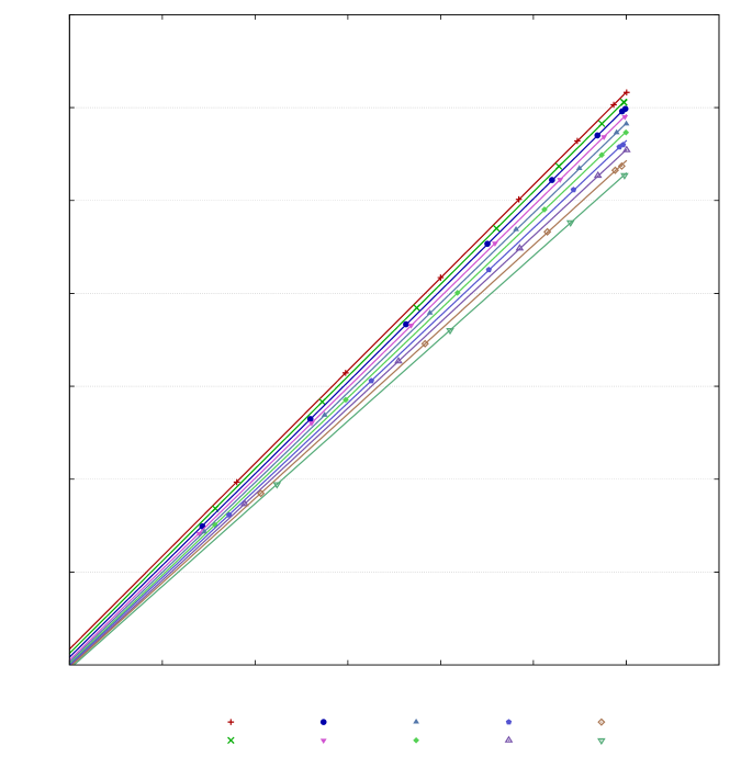
0.00.00.00.20.20.20.40.40.40.60.60.60.80.80.81.01.01.01.21.21.21.41.41.40.00.00.00.20.20.20.40.40.40.60.60.60.80.80.81.01.01.01.21.21.21.41.41.4zLW= 0.9990zFLRW+ 0.0342,subscript𝑧𝐿𝑊0.9990subscript𝑧𝐹𝐿𝑅𝑊0.0342z_{\scriptscriptstyle LW}\,=\,0.9990\,z_{\scriptscriptstyle FLRW}\,+\,0.0342,RMS of residuals= 8.461×10⁴RMS of residuals8.461superscript104\text{RMS of residuals}\,=\,8.461\times 10^{-4}zLW= 0.9935zFLRW+ 0.0251,subscript𝑧𝐿𝑊0.9935subscript𝑧𝐹𝐿𝑅𝑊0.0251z_{\scriptscriptstyle LW}\,=\,0.9935\,z_{\scriptscriptstyle FLRW}\,+\,0.0251,RMS of residuals= 1.141×10³RMS of residuals1.141superscript103\text{RMS of residuals}\,=\,1.141\times 10^{-3}zLW= 0.9866zFLRW+ 0.0170,subscript𝑧𝐿𝑊0.9866subscript𝑧𝐹𝐿𝑅𝑊0.0170z_{\scriptscriptstyle LW}\,=\,0.9866\,z_{\scriptscriptstyle FLRW}\,+\,0.0170,RMS of residuals= 1.116×10³RMS of residuals1.116superscript103\text{RMS of residuals}\,=\,1.116\times 10^{-3}zLW= 0.9781zFLRW+ 0.0105,subscript𝑧𝐿𝑊0.9781subscript𝑧𝐹𝐿𝑅𝑊0.0105z_{\scriptscriptstyle LW}\,=\,0.9781\,z_{\scriptscriptstyle FLRW}\,+\,0.0105,RMS of residuals= 7.763×10⁴RMS of residuals7.763superscript104\text{RMS of residuals}\,=\,7.763\times 10^{-4}zLW= 0.9665zFLRW+ 0.0063,subscript𝑧𝐿𝑊0.9665subscript𝑧𝐹𝐿𝑅𝑊0.0063z_{\scriptscriptstyle LW}\,=\,0.9665\,z_{\scriptscriptstyle FLRW}\,+\,0.0063,RMS of residuals= 9.523×10⁴RMS of residuals9.523superscript104\text{RMS of residuals}\,=\,9.523\times 10^{-4}zLW= 0.9547zFLRW+ 0.0024,subscript𝑧𝐿𝑊0.9547subscript𝑧𝐹𝐿𝑅𝑊0.0024z_{\scriptscriptstyle LW}\,=\,0.9547\,z_{\scriptscriptstyle FLRW}\,+\,0.0024,RMS of residuals= 7.152×10⁴RMS of residuals7.152superscript104\text{RMS of residuals}\,=\,7.152\times 10^{-4}zLW= 0.9404zFLRW+ 0.0000,subscript𝑧𝐿𝑊0.9404subscript𝑧𝐹𝐿𝑅𝑊0.0000z_{\scriptscriptstyle LW}\,=\,0.9404\,z_{\scriptscriptstyle FLRW}\,+\,0.0000,RMS of residuals= 1.422×10³RMS of residuals1.422superscript103\text{RMS of residuals}\,=\,1.422\times 10^{-3}zLW= 0.9267zFLRW 0.0032,subscript𝑧𝐿𝑊0.9267subscript𝑧𝐹𝐿𝑅𝑊0.0032z_{\scriptscriptstyle LW}\,=\,0.9267\,z_{\scriptscriptstyle FLRW}\,-\,0.0032,RMS of residuals= 9.969×10⁴RMS of residuals9.969superscript104\text{RMS of residuals}\,=\,9.969\times 10^{-4}zLW= 0.9085zFLRW 0.0049,subscript𝑧𝐿𝑊0.9085subscript𝑧𝐹𝐿𝑅𝑊0.0049z_{\scriptscriptstyle LW}\,=\,0.9085\,z_{\scriptscriptstyle FLRW}\,-\,0.0049,RMS of residuals= 1.946×10³RMS of residuals1.946superscript103\text{RMS of residuals}\,=\,1.946\times 10^{-3}zLW= 0.8892zFLRW 0.0085,subscript𝑧𝐿𝑊0.8892subscript𝑧𝐹𝐿𝑅𝑊0.0085z_{\scriptscriptstyle LW}\,=\,0.8892\,z_{\scriptscriptstyle FLRW}\,-\,0.0085,RMS of residuals= 8.650×10⁴RMS of residuals8.650superscript104\text{RMS of residuals}\,=\,8.650\times 10^{-4}Refer to caption

zLWsubscript𝑧𝐿𝑊z_{\scriptscriptstyle LW}

zFLRWsubscript𝑧𝐹𝐿𝑅𝑊z_{\scriptscriptstyle FLRW}1.57081.57081.57081.44511.44511.44511.31951.31951.31951.19381.19381.19381.06811.06811.06810.94250.94250.94250.81680.81680.81680.69120.69120.69120.56550.56550.56550.43980.43980.4398
Figure 27: A plot of zLWsubscript𝑧𝐿𝑊z_{\scriptscriptstyle LW} against zFLRWsubscript𝑧𝐹𝐿𝑅𝑊z_{\scriptscriptstyle FLRW} while photons are outgoing. Graphs for a selection of photon trajectories θnsubscript𝜃𝑛\theta_{n} are shown. A linear regression was performed on each graph, and the regression equation is listed in order of decreasing θnsubscript𝜃𝑛\theta_{n}.
0.80.8-0.80.60.6-0.60.40.4-0.40.20.2-0.20.00.00.00.20.20.20.40.40.40.60.60.60.80.80.81.01.01.01.21.21.21.41.41.40.60.6-0.60.40.4-0.40.20.2-0.20.00.00.00.20.20.20.40.40.40.60.60.60.80.80.81.01.01.01.21.21.21.41.41.4zLW= 1.0271zFLRW 0.0028,subscript𝑧𝐿𝑊1.0271subscript𝑧𝐹𝐿𝑅𝑊0.0028z_{\scriptscriptstyle LW}\,=\,1.0271\,z_{\scriptscriptstyle FLRW}\,-\,0.0028,RMS of residuals= 1.552×10³RMS of residuals1.552superscript103\text{RMS of residuals}\,=\,1.552\times 10^{-3}zLW= 1.0201zFLRW 0.0098,subscript𝑧𝐿𝑊1.0201subscript𝑧𝐹𝐿𝑅𝑊0.0098z_{\scriptscriptstyle LW}\,=\,1.0201\,z_{\scriptscriptstyle FLRW}\,-\,0.0098,RMS of residuals= 6.617×10⁴RMS of residuals6.617superscript104\text{RMS of residuals}\,=\,6.617\times 10^{-4}zLW= 1.0128zFLRW 0.0173,subscript𝑧𝐿𝑊1.0128subscript𝑧𝐹𝐿𝑅𝑊0.0173z_{\scriptscriptstyle LW}\,=\,1.0128\,z_{\scriptscriptstyle FLRW}\,-\,0.0173,RMS of residuals= 6.439×10⁴RMS of residuals6.439superscript104\text{RMS of residuals}\,=\,6.439\times 10^{-4}zLW= 1.0060zFLRW 0.0260,subscript𝑧𝐿𝑊1.0060subscript𝑧𝐹𝐿𝑅𝑊0.0260z_{\scriptscriptstyle LW}\,=\,1.0060\,z_{\scriptscriptstyle FLRW}\,-\,0.0260,RMS of residuals= 1.085×10³RMS of residuals1.085superscript103\text{RMS of residuals}\,=\,1.085\times 10^{-3}zLW= 1.0008zFLRW 0.0375,subscript𝑧𝐿𝑊1.0008subscript𝑧𝐹𝐿𝑅𝑊0.0375z_{\scriptscriptstyle LW}\,=\,1.0008\,z_{\scriptscriptstyle FLRW}\,-\,0.0375,RMS of residuals= 6.022×10⁴RMS of residuals6.022superscript104\text{RMS of residuals}\,=\,6.022\times 10^{-4}zLW= 0.9955zFLRW 0.0491,subscript𝑧𝐿𝑊0.9955subscript𝑧𝐹𝐿𝑅𝑊0.0491z_{\scriptscriptstyle LW}\,=\,0.9955\,z_{\scriptscriptstyle FLRW}\,-\,0.0491,RMS of residuals= 9.149×10⁴RMS of residuals9.149superscript104\text{RMS of residuals}\,=\,9.149\times 10^{-4}zLW= 0.9891zFLRW 0.0605,subscript𝑧𝐿𝑊0.9891subscript𝑧𝐹𝐿𝑅𝑊0.0605z_{\scriptscriptstyle LW}\,=\,0.9891\,z_{\scriptscriptstyle FLRW}\,-\,0.0605,RMS of residuals= 9.778×10⁴RMS of residuals9.778superscript104\text{RMS of residuals}\,=\,9.778\times 10^{-4}zLW= 0.9821zFLRW 0.0718,subscript𝑧𝐿𝑊0.9821subscript𝑧𝐹𝐿𝑅𝑊0.0718z_{\scriptscriptstyle LW}\,=\,0.9821\,z_{\scriptscriptstyle FLRW}\,-\,0.0718,RMS of residuals= 1.498×10³RMS of residuals1.498superscript103\text{RMS of residuals}\,=\,1.498\times 10^{-3}zLW= 0.9700zFLRW 0.0805,subscript𝑧𝐿𝑊0.9700subscript𝑧𝐹𝐿𝑅𝑊0.0805z_{\scriptscriptstyle LW}\,=\,0.9700\,z_{\scriptscriptstyle FLRW}\,-\,0.0805,RMS of residuals= 1.517×10³RMS of residuals1.517superscript103\text{RMS of residuals}\,=\,1.517\times 10^{-3}zLW= 0.9525zFLRW 0.0870,subscript𝑧𝐿𝑊0.9525subscript𝑧𝐹𝐿𝑅𝑊0.0870z_{\scriptscriptstyle LW}\,=\,0.9525\,z_{\scriptscriptstyle FLRW}\,-\,0.0870,RMS of residuals= 1.710×10³RMS of residuals1.710superscript103\text{RMS of residuals}\,=\,1.710\times 10^{-3}Refer to caption

zLWsubscript𝑧𝐿𝑊z_{\scriptscriptstyle LW}

zFLRWsubscript𝑧𝐹𝐿𝑅𝑊z_{\scriptscriptstyle FLRW}1.57081.57081.57081.44511.44511.44511.31951.31951.31951.19381.19381.19381.06811.06811.06810.94250.94250.94250.81680.81680.81680.69120.69120.69120.56550.56550.56550.43980.43980.4398
Figure 28: A plot of zLWsubscript𝑧𝐿𝑊z_{\scriptscriptstyle LW} against zFLRWsubscript𝑧𝐹𝐿𝑅𝑊z_{\scriptscriptstyle FLRW} while photons are ingoing. Graphs for the same trajectories as in Fig. 27 are shown. A linear regression was performed on each graph, and the regression equation is listed in order of decreasing θnsubscript𝜃𝑛\theta_{n}. Though in this case, the regression only includes redshifts measured at robssubscript𝑟𝑜𝑏𝑠r_{obs} equal to at least 10R10𝑅10\,R, the photon’s starting radius, so as to exclude points in the initial bend.

In Fig. 29, we have plotted the gradients of zLWsubscript𝑧𝐿𝑊z_{\scriptscriptstyle LW} vs zFLRWsubscript𝑧𝐹𝐿𝑅𝑊z_{\scriptscriptstyle FLRW} against cos(θn)subscript𝜃𝑛\cos(\theta_{n}).

0.860.860.860.890.890.890.920.920.920.950.950.950.980.980.981.011.011.011.041.041.040.00.00.00.10.10.10.20.20.20.30.30.30.40.40.40.50.50.50.60.60.60.70.70.70.80.80.80.90.90.91.01.01.0

gradient of zLWsubscript𝑧𝐿𝑊z_{\scriptscriptstyle LW} vs zFLRWsubscript𝑧𝐹𝐿𝑅𝑊z_{\scriptscriptstyle FLRW}

cos(θ)𝜃\cos(\theta)Refer to captionoutgoingingoing
Figure 29: A plot of zLWsubscript𝑧𝐿𝑊z_{\scriptscriptstyle LW} vs zFLRWsubscript𝑧𝐹𝐿𝑅𝑊z_{\scriptscriptstyle FLRW} gradients against cos(θn)subscript𝜃𝑛\cos(\theta_{n}), where θnsubscript𝜃𝑛\theta_{n} is the initial direction of the photon. The gradients for when the photons are outgoing and for when they are ingoing are plotted separately, and all gradients are obtained by performing a linear regression on zLWsubscript𝑧𝐿𝑊z_{\scriptscriptstyle LW} vs zFLRWsubscript𝑧𝐹𝐿𝑅𝑊z_{\scriptscriptstyle FLRW} data. To avoid the initial bend in the zLWsubscript𝑧𝐿𝑊z_{\scriptscriptstyle LW} vs zFLRWsubscript𝑧𝐹𝐿𝑅𝑊z_{\scriptscriptstyle FLRW} graphs for ingoing photons, the ingoing gradients are obtained by regressing over only data points for which robssubscript𝑟𝑜𝑏𝑠r_{obs} is at least equal to the photon’s starting radius of 10R10𝑅10\,R.

Two graphs are shown, one for the gradients when the photons are outgoing, and the other for when they are ingoing. To exclude the initial bend in the graphs for ingoing photons, we excluded data points corresponding to robssubscript𝑟𝑜𝑏𝑠r_{obs} less than 10R10𝑅10\,R, the photons’ starting radius.151515In fact, including all data points in the regression introduced some ‘jaggedness’ in the graph of ingoing gradients, especially towards the low cos(θn)subscript𝜃𝑛\cos(\theta_{n}) regime. By excluding these points, the ‘jaggedness’ smoothed away, and we were left with a curve much more similar to that for the outgoing gradients. The figure shows that, as with the other universes, the gradient decreases as the photon’s trajectory becomes more radial, but now, the relationship between the gradients and cos(θn)subscript𝜃𝑛\cos(\theta_{n}) is no longer linear.

Thus to summarise, our simulations have demonstrated several features common to redshifts in all LW universes. The LW redshifts generally increase linearly with their FLRW counterparts in any universe and for any photon trajectory. When robssubscript𝑟𝑜𝑏𝑠r_{obs} is small such that the central mass has a stronger influence, there is some deviation away from this linear behaviour. Any influence from the central mass can be suppressed by starting the photon at very large radii; zLWsubscript𝑧𝐿𝑊z_{\scriptscriptstyle LW} then becomes completely proportional to zFLRWsubscript𝑧𝐹𝐿𝑅𝑊z_{\scriptscriptstyle FLRW}. The LW redshifts also generally decrease relative to their FLRW counterparts as the photon takes a more radial trajectory; this can also be attributed to the stronger influence of the central mass since a more radial trajectory would pass closer to it. The mass’ influence on redshifts can sometimes be quite significant, causing LW redshifts to deviate from their FLRW counterparts by as much as 30%. This would have significant implications if we attempted to fit redshift data from a lattice universe onto an FLRW model, as quantities such as the age of the universe may be incorrectly estimated. Thus we see certain significant effects arising from the ‘lumpiness’ of the LW universe which an FLRW-based model could not adequately capture.

This influence of the masses on redshifts can be understood as an integrated Sachs-Wolfe effect (ISW). The ISW describes the net redshift induced on a photon as it passes through a fluctuating gravitational potential caused by fluctuations in the energy density (Sachs and Wolfe, 1967; Rees and Sciama, 1968; Martínez-González et al., 1990; Nishizawa, 2014). In a flat FLRW universe, a time-varying potential is necessary to generate a non-zero ISW; however when the universe is matter-dominated, the potential is static, and therefore the ISW would be zero. If there is a non-zero cosmological constant though, the potential in a matter-dominated universe does become time-varying, and hence a non-zero ISW can result (Crittenden and Turok, 1996). Indeed, recent precision observations of the cosmos have not only established that our universe is very nearly flat but that there is definitely a non-zero ISW (Boughn and Crittenden, 2004; Planck collaboration, 2015); naturally, this has been interpreted as evidence of a non-zero cosmological constant in our universe. However, our results suggest that this might be explainable within a matter-dominated universe without needing a cosmological constant; we may simply require a model that better reflects the inhomogeneous matter distribution than FLRW space-times allow. Because of the significant implications a non-zero ISW may have on the dark energy question, this modelling problem deserves further investigation.

VIII.   Discussion

We have investigated the properties of the Lindquist-Wheeler universes, as we hope they might provide some insight into what observable effects the ‘lumpy’ matter distribution of the actual universe might yield. And although the LW universes are only approximations rather than exact solutions to the Einstein equations, we believe they model enough of the underlying physics to yield at least meaningful qualitative insights into the behaviour of the actual universe. Much of the LW universes’ dynamics bear strong resemblance to those of the matter-dominated FLRW universes. Additionally, photon redshifts in LW universes behaved roughly similarly to their FLRW counterparts. Yet there were also certain direction-dependent effects in the redshifts due to the ‘lumpiness’ of the universe’s matter distribution.

We noted that there were some differences between Clifton and Ferreira’s results and ours for the flat universe. Most notably, our redshifts displayed the effects of the inhomogeneous matter distribution more. The effects became stronger the closer the photon passed to a mass and the more radial the photon’s trajectory was. As a result, our redshifts demonstrated a non-zero ISW, which was not present in Clifton and Ferreira’s results. Otherwise, when the photon was far from any mass, its redshift would behave much more similarly to FLRW redshifts as well as to Clifton and Ferreira’s mean redshift relation. The main difference between Clifton and Ferreira’s model and ours was the definition of the cell boundary and the choice of conditions for propagating particles across boundaries. As Clifton and Ferreira have shown, these can significantly alter the redshift relations; for instance, using a different choice of boundary conditions, Clifton and Ferreira obtained the redshift relation of 1+zLW(1+zFLRW)7/101subscript𝑧𝐿𝑊superscript1subscript𝑧𝐹𝐿𝑅𝑊7101+z_{\scriptscriptstyle LW}\approx(1+z_{\scriptscriptstyle FLRW})^{7/10} instead (Clifton and Ferreira, 2009a; Clifton et al., 2012b), which clearly agreed far less with FLRW redshifts. Further investigation is required to determine whether our discrepancy from Clifton and Ferreira’s results is indeed significant or merely an artefact of our boundary conditions which somehow exaggerates the effects of the masses. Nevertheless, neither our inhomogeneous results nor Clifton and Ferreira’s more homogeneous one can be ruled out at the moment.

There are several ways in which our investigation can be extended. It would be interesting to examine the optical properties of the LW universe, as this may have important implications for actual astrophysical observations. Clifton and Ferreira have already done this for their implementation of the LW universe, but we have used a different implementation from theirs, and this has led to certain differences in the behaviour of redshifts. However, Clifton and Ferreira have suggested that the optical properties, unlike the redshifts, may actually be insensitive to the choice of boundary conditions (Clifton et al., 2012b). Nevertheless, it would be very interesting to see whether that is indeed the case for our boundary conditions. It would also be interesting to extend our study to LW universes with a non-zero cosmological constant and attempt to evaluate by how much inhomogeneities reduce the need for such a constant. Clifton and Ferreira have already constructed an appropriate extension of the LW universe based on the Schwarzschild de-Sitter metric, and they have shown that the corresponding Friedmann-like equation strongly resembles its FLRW counterpart as well. Moreover, using their boundary conditions, they have also shown that the cosmological constant density ratio ΩΛsubscriptΩΛ\Omega_{\Lambda} can be reduced by about 10% (Clifton and Ferreira, 2009b; Clifton et al., 2012b), and again this was rather insensitive to which boundary condition they used. It should be possible to include Clifton and Ferreira’s ΛΛ\Lambda-Schwarzschild-cells in our implementation and to investigate the resulting model. Finally, our model has a still very idealised distribution of matter. Each mass is identical and distributed on a perfect lattice which is clearly not the case in the actual universe. We should like to extend our model to allow for different sized masses and cells. To this end, we have derived in Appendix D a set of conditions that must be satisfied at the boundary between two neighbouring cells of different mass m𝑚m. We leave the numerical simulation of such universes and the detailed investigation of their properties to future work.

Acknowledgements.
The author would like to thank Ruth Williams, Timothy Clifton, Pedro Ferreira, and Ulrich Sperhake for much helpful discussion. Timothy and Ulrich pointed out to the author the resemblance between the paper’s redshift results and the integrated Sachs-Wolfe effect. The numerical simulations of the Lindquist-Wheeler models were performed on the COSMOS Shared Memory system at DAMTP, University of Cambridge, operated on behalf of the STFC DiRAC HPC Facility. This equipment is funded by BIS National E-infrastructure capital grant ST/J005673/1 and STFC grants ST/H008586/1, ST/K00333X/1, and ST/J001341/1. The author also wishes to thank the COSMOS team, in general, for technical support and James Briggs, in particular, for his kind assistance in parallelising the C++ code with OpenMP. The author was financed in part by a bursary from the Cambridge Commonwealth Trust.

Appendix A Regular lattices in 3-spaces of constant curvature

In this appendix, we shall list all possible lattices that cover 3-spaces of constant curvature with a single regular polyhedral cell. The cell is tiled to completely cover the 3-space without any gaps or overlaps. This tessellation problem has been thoroughly studied by Coxeter (Coxeter, 1948). Clifton and Ferreira (Clifton and Ferreira, 2009a) have succinctly summarised Coxeter’s results relevant to our discussion, and we have presented their summary in Table 3.

Table 3: All possible lattices obtained by tessellating 3-spaces of constant curvature with a single regular polyhedron.
Elementary cell shape Number of cells at a lattice edge Background curvature Total cells in lattice
tetrahedron 3 + 5
cube 3 + 8
tetrahedron 4 + 16
octahedron 3 + 24
dodecahedron 3 + 120
tetrahedron 5 + 600
cube 4 0 \infty
cube 5 - \infty
dodecahedron 4 - \infty
dodecahedron 5 - \infty
icosahedron 3 - \infty

Column 1 gives the lattice cell’s shape. Column 2 effectively determines the lattice’s structure: it indicates how many of Column 1’s elementary cells meet at any lattice edge. Column 3 indicates whether the background 3-space has positive, flat, or negative curvature. Column 4 gives the number of cells needed to cover the 3-space; only lattices on positively curved space can have a finite number of cells. To construct a closed lattice universe, one has six choices of lattices; for example, one can choose a 600-cell lattice where cells are equilateral tetrahedra and where five tetrahedra meet at any edge. To construct a flat lattice, one has but a single choice. To construct an open lattice, one has four.

Appendix B Radial velocities in Regge space-time
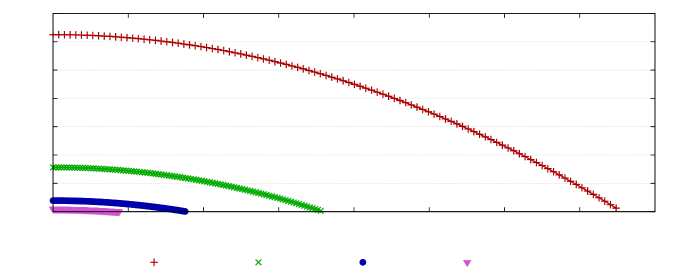
0.000.000.000.020.020.020.040.040.040.060.060.060.080.080.080.100.100.100.120.120.120.140.140.140.000.000.000.050.050.050.100.100.100.150.150.150.200.200.200.250.250.250.300.300.300.350.350.350.400.400.40

R/rmax𝑅subscript𝑟𝑚𝑎𝑥R/r_{max}

ρ˙initsubscript˙𝜌𝑖𝑛𝑖𝑡\dot{\rho}_{init}R/rmax=0.8750(ρ˙init)2+ 0.1250𝑅subscript𝑟𝑚𝑎𝑥0.8750superscriptsubscript˙𝜌𝑖𝑛𝑖𝑡20.1250R/r_{max}\,=\,-0.8750(\dot{\rho}_{init})^{2}\,+\,0.1250RMS of residuals= 2.51×10⁷RMS of residuals2.51superscript107\text{RMS of residuals}\,=\,2.51\times 10^{-7}R/rmax=0.9688(ρ˙init)2+ 0.0313𝑅subscript𝑟𝑚𝑎𝑥0.9688superscriptsubscript˙𝜌𝑖𝑛𝑖𝑡20.0313R/r_{max}\,=\,-0.9688(\dot{\rho}_{init})^{2}\,+\,0.0313RMS of residuals= 5.04×10⁸RMS of residuals5.04superscript108\text{RMS of residuals}\,=\,5.04\times 10^{-8}R/rmax=0.9922(ρ˙init)2+ 0.0078𝑅subscript𝑟𝑚𝑎𝑥0.9922superscriptsubscript˙𝜌𝑖𝑛𝑖𝑡20.0078R/r_{max}\,=\,-0.9922(\dot{\rho}_{init})^{2}\,+\,0.0078RMS of residuals= 8.13×10⁹RMS of residuals8.13superscript109\text{RMS of residuals}\,=\,8.13\times 10^{-9}R/rmax=0.9981(ρ˙init)2+ 0.0020𝑅subscript𝑟𝑚𝑎𝑥0.9981superscriptsubscript˙𝜌𝑖𝑛𝑖𝑡20.0020R/r_{max}\,=\,-0.9981(\dot{\rho}_{init})^{2}\,+\,0.0020RMS of residuals= 1.94×10⁸RMS of residuals1.94superscript108\text{RMS of residuals}\,=\,1.94\times 10^{-8}Refer to captionrinit/R=8subscript𝑟𝑖𝑛𝑖𝑡𝑅8r_{init}/R=8rinit/R=32subscript𝑟𝑖𝑛𝑖𝑡𝑅32r_{init}/R=32rinit/R=128subscript𝑟𝑖𝑛𝑖𝑡𝑅128r_{init}/R=128rinit/R=512subscript𝑟𝑖𝑛𝑖𝑡𝑅512r_{init}/R=512
Figure 30: A plot of R/rmax𝑅subscript𝑟𝑚𝑎𝑥R/r_{max} versus ρ˙initsubscript˙𝜌𝑖𝑛𝑖𝑡\dot{\rho}_{init} for various rinitsubscript𝑟𝑖𝑛𝑖𝑡r_{init}. Each graph has 100 data points. A quadratic regression has been performed on each graph, and the regression equations are ordered from rinit=8Rsubscript𝑟𝑖𝑛𝑖𝑡8𝑅r_{init}=8\,R to 512R512𝑅512\,R. The regressions were performed without a linear term; regression was also attempted with a linear term present, but it was found to be many orders of magnitude smaller than the other two terms. The simulation’s block parameters were R=31𝑅31R=31, Δt=10ΔrΔ𝑡10Δ𝑟\Delta t=10\Delta r, Δr=R/105Δ𝑟𝑅superscript105\Delta r=R/10^{5}, and Δϕ=2π/(3×107)Δitalic-ϕ2𝜋3superscript107\Delta\phi=2\pi/(3\times 10^{7}).
0.00.00.00.20.20.20.40.40.40.60.60.60.80.80.81.01.01.01.21.21.20.00.00.00.20.20.20.40.40.40.60.60.60.80.80.81.01.01.01.21.21.2

(uρ)2superscriptsuperscript𝑢𝜌2(u^{\rho})^{2}

(ρ˙)2superscript˙𝜌2(\dot{\rho})^{2}uρ=ρ˙ 3.9×10⁶superscript𝑢𝜌˙𝜌3.9superscript106u^{\rho}\,=\,\dot{\rho}\,-\,3.9\times 10^{-6}RMS of residuals= 1.86×10⁷RMS of residuals1.86superscript107\text{RMS of residuals}\,=\,1.86\times 10^{-7}uρ=ρ˙ 3.0×10⁶superscript𝑢𝜌˙𝜌3.0superscript106u^{\rho}\,=\,\dot{\rho}\,-\,3.0\times 10^{-6}RMS of residuals= 1.04×10⁷RMS of residuals1.04superscript107\text{RMS of residuals}\,=\,1.04\times 10^{-7}uρ=ρ˙ 2.6×10⁶superscript𝑢𝜌˙𝜌2.6superscript106u^{\rho}\,=\,\dot{\rho}\,-\,2.6\times 10^{-6}RMS of residuals= 8.41×10⁸RMS of residuals8.41superscript108\text{RMS of residuals}\,=\,8.41\times 10^{-8}uρ=ρ˙ 2.5×10⁶superscript𝑢𝜌˙𝜌2.5superscript106u^{\rho}\,=\,\dot{\rho}\,-\,2.5\times 10^{-6}RMS of residuals= 7.96×10⁸RMS of residuals7.96superscript108\text{RMS of residuals}\,=\,7.96\times 10^{-8}uρ=ρ˙ 2.6×10⁶superscript𝑢𝜌˙𝜌2.6superscript106u^{\rho}\,=\,\dot{\rho}\,-\,2.6\times 10^{-6}RMS of residuals= 6.76×10⁸RMS of residuals6.76superscript108\text{RMS of residuals}\,=\,6.76\times 10^{-8}Refer to captionR/rmax=1/11𝑅subscript𝑟𝑚𝑎𝑥111R/r_{max}=-1/11R/rmax=1/31𝑅subscript𝑟𝑚𝑎𝑥131R/r_{max}=-1/31R/rmax=1/51𝑅subscript𝑟𝑚𝑎𝑥151R/r_{max}=-1/51R/rmax=1/71𝑅subscript𝑟𝑚𝑎𝑥171R/r_{max}=-1/71R/rmax=1/91𝑅subscript𝑟𝑚𝑎𝑥191R/r_{max}=-1/91
Figure 31: A plot of (uρ)2superscriptsuperscript𝑢𝜌2(u^{\rho})^{2} against ρ~˙ 2superscript˙~𝜌2\dot{\tilde{\rho}}^{\,2} for various rmax<0subscript𝑟𝑚𝑎𝑥0r_{max}<0, where uρsuperscript𝑢𝜌u^{\rho} is given by (44). Each plot consists of velocities computed at 100 different radii along the course of the test particle’s trajectory. A linear regression was performed on each graph, and the corresponding equations are ordered from R/rmax=1/11𝑅subscript𝑟𝑚𝑎𝑥111R/r_{max}=-1/11 to 1/91191-1/91. The graphs of the regressions completely overlap each other. The gradients only begin deviating from unity at the 105superscript10510^{-5} order of magnitude. The simulation’s block parameters were rinit=2Rsubscript𝑟𝑖𝑛𝑖𝑡2𝑅r_{init}=2\,R, R=21𝑅21R=21, Δt=Δr=R/105Δ𝑡Δ𝑟𝑅superscript105\Delta t=\Delta r=R/10^{5}, and Δϕ=2π/(3×107)Δitalic-ϕ2𝜋3superscript107\Delta\phi=2\pi/(3\times 10^{7}).

In this appendix, we shall present our numerical results supporting (44) to be the 4-velocity tangent to radial time-like geodesics in Regge Schwarzschild space-time. These geodesics include, most importantly, those of test particles co-moving with a Schwarzschild-cell boundary. We began by determining numerically the escape velocity for a test particle. We propagated a test particle radially outwards from a series of initial radii rinitsubscript𝑟𝑖𝑛𝑖𝑡r_{init} and with a series of initial velocities ρ˙initsubscript˙𝜌𝑖𝑛𝑖𝑡\dot{\rho}_{init}. We started ρ˙initsubscript˙𝜌𝑖𝑛𝑖𝑡\dot{\rho}_{init} from 0 and increased it until the maximum radius rmaxsubscript𝑟𝑚𝑎𝑥r_{max} attained by the particle was very large. For each rinitsubscript𝑟𝑖𝑛𝑖𝑡r_{init}, we then plotted R/rmax𝑅subscript𝑟𝑚𝑎𝑥R/r_{max} against its corresponding ρ˙initsubscript˙𝜌𝑖𝑛𝑖𝑡\dot{\rho}_{init}, where R𝑅R is the Schwarzschild radius. Both rinitsubscript𝑟𝑖𝑛𝑖𝑡r_{init} and rmaxsubscript𝑟𝑚𝑎𝑥r_{max} refer to the lower Schwarzschild label of the block in which the particle is found. Our plots are shown in Fig. 30. Each graph is very well-fitted by a quadratic curve of the form

Rrmax=Aρ˙init2+B.𝑅subscript𝑟𝑚𝑎𝑥𝐴superscriptsubscript˙𝜌𝑖𝑛𝑖𝑡2𝐵\frac{R}{r_{max}}=-A\,\dot{\rho}_{init}^{2}+B.

Moreover, the co-efficients A𝐴A and B𝐵B always satisfy the relations A+B=1𝐴𝐵1A+B=1 and B=R/rinit𝐵𝑅subscript𝑟𝑖𝑛𝑖𝑡B=R/r_{init}.161616We have also looked at graphs for different R𝑅R and rinitsubscript𝑟𝑖𝑛𝑖𝑡r_{init}, not shown, and they also conform to this pattern. From these relations, we can therefore infer a relation for ρ˙˙𝜌\dot{\rho} corresponding to that given in (44), and the τ˙˙𝜏\dot{\tau} component follows from normalisation.

0020202040404060606080808010010010012012012014014014016016016018018018000500050005000100001000010000150001500015000200002000020000250002500025000300003000030000

1/ρ˙1˙𝜌1/\dot{\rho}

r/R𝑟𝑅r/RRefer to captionΔr=R/101Δ𝑟𝑅superscript101\Delta r=R/10^{1}Δr=R/102Δ𝑟𝑅superscript102\Delta r=R/10^{2}Δr=R/103Δ𝑟𝑅superscript103\Delta r=R/10^{3}Δr=R/104Δ𝑟𝑅superscript104\Delta r=R/10^{4}Δr=R/105Δ𝑟𝑅superscript105\Delta r=R/10^{5}uρsuperscript𝑢𝜌u^{\rho}
Figure 32: A plot of 1/ρ˙1˙𝜌1/\dot{\rho} versus r/R𝑟𝑅r/R comparing simulated particle velocities with uρsuperscript𝑢𝜌u^{\rho}. For the simulated particles’ graphs ρ˙=ρ~˙˙𝜌˙~𝜌\dot{\rho}=\dot{\tilde{\rho}}, while for the uρsuperscript𝑢𝜌u^{\rho} graph, ρ˙=uρ˙𝜌superscript𝑢𝜌\dot{\rho}=u^{\rho}. The simulation was run for various sizes ΔrΔ𝑟\Delta r of the Regge block. For all simulations, the particle was propagated from r=2R𝑟2𝑅r=2\,R to 3×10⁴R3superscript104𝑅3\times 10^{4}\,R. The simulation’s other block parameters were R=1𝑅1R=1, Δt=ΔrΔ𝑡Δ𝑟\Delta t=\Delta r, and Δϕ=2π/(3×107)Δitalic-ϕ2𝜋3superscript107\Delta\phi=2\pi/(3\times 10^{7}).

We have just provided numerical support for (44) for test particles following geodesics where rmax0subscript𝑟𝑚𝑎𝑥0r_{max}\geq 0, corresponding to closed orbits or orbits at the escape velocity. At this point, we conjectured that for open orbits, (44) would still apply but with rmax<0subscript𝑟𝑚𝑎𝑥0r_{max}<0. To test this, we propagated a test particle outwards with an initial velocity given by (44) but for rmax<0subscript𝑟𝑚𝑎𝑥0r_{max}<0, and we examined how the velocity evolved with r𝑟r. Let us denote the velocity of our simulated particle by ρ~˙˙~𝜌\dot{\tilde{\rho}}. Along the particle’s trajectory, we compared ρ~˙ 2superscript˙~𝜌2\dot{\tilde{\rho}}^{\,2} against (uρ)2superscriptsuperscript𝑢𝜌2(u^{\rho})^{2} for the same radius, where uρsuperscript𝑢𝜌u^{\rho} is given by the radial component of (44). Our comparison is presented graphically in Fig. 31. In all cases, the graphs’ gradients were effectively unity and the constants effectively zero, thus indicating that the particle’s velocity does indeed obey (44). In Table 4, we provide a partial list of the values of ρ~˙ 2superscript˙~𝜌2\dot{\tilde{\rho}}^{\,2} and (uρ)2superscriptsuperscript𝑢𝜌2(u^{\rho})^{2} as well as their percentage difference. The percentage difference is very small in all rows, although there appears to be an increasing trend with increasing r𝑟r. We find that our conjecture is supported by numerical results, and hence (44) appears valid for all types of radial time-like geodesics.171717Again, we have also simulated the cases of rmax=R,21R,41R,61R,subscript𝑟𝑚𝑎𝑥𝑅21𝑅41𝑅61𝑅r_{max}=-R,-21\,R,-41\,R,-61\,R, and 81R81𝑅-81\,R, not shown here, and they all display the same behaviour as in Fig. 31. The percentage difference seen between ρ~˙ 2superscript˙~𝜌2\dot{\tilde{\rho}}^{\,2} and (uρ)2superscriptsuperscript𝑢𝜌2(u^{\rho})^{2} is also small but slowly increasing in all rmaxsubscript𝑟𝑚𝑎𝑥r_{max} that we looked at.

Table 4: A list of ρ~˙ 2superscript˙~𝜌2\dot{\tilde{\rho}}^{\,2} and (uρ)2superscriptsuperscript𝑢𝜌2(u^{\rho})^{2} at various radii, and the percentage difference between them. This data is for R/rmax=91𝑅subscript𝑟𝑚𝑎𝑥91R/r_{max}=-91.
r/R𝑟𝑅r/R ρ~˙ 2superscript˙~𝜌2\dot{\tilde{\rho}}^{\,2} (uρ)2superscriptsuperscript𝑢𝜌2(u^{\rho})^{2} % difference
2 1.02197946491.02197946491.0219794649 1.021978021978021.021978021978021.02197802197802 0.000141188940473120.000141188940473120.00014118894047312
102 0.0210012267240.0210012267240.021001226724 0.02099880155959720.02099880155959720.0209988015595972 0.01154772735283820.01154772735283820.0115477273528382
202 0.0160212306250.0160212306250.016021230625 0.01601881211840310.01601881211840310.0160188121184031 0.01509563561916020.01509563561916020.0150956356191602
302 0.0143503628490.0143503628490.014350362849 0.01434778021974140.01434778021974140.0143477802197414 0.01799696137137850.01799696137137850.0179969613713785
402 0.0135126675360.0135126675360.013512667536 0.01351017836831290.01351017836831290.0135101783683129 0.01842099408201870.01842099408201870.0184209940820187
502 0.0130094554810.0130094554810.013009455481 0.01300695122606180.01300695122606180.0130069512260618 0.01924949850371110.01924949850371110.0192494985037111
602 0.0126738060840.0126738060840.012673806084 0.01267118948199520.01267118948199520.0126711894819952 0.02064574751609020.02064574751609020.0206457475160902
702 0.0124338110490.0124338110490.012433811049 0.01243121926084810.01243121926084810.0124312192608481 0.02084468021684330.02084468021684330.0208446802168433
802 0.0122536044160.0122536044160.012253604416 0.01225116672377550.01225116672377550.0122511667237755 0.01989367488709440.01989367488709440.0198936748870944
\vdots \vdots \vdots \vdots
9202 0.0111015724960.0111015724960.011101572496 0.01109888912749030.01109888912749030.0110988891274903 0.02417106685304010.02417106685304010.0241710668530401
9302 0.0111003081640.0111003081640.011100308164 0.01109770803701580.01109770803701580.0110977080370158 0.02342391711817740.02342391711817740.0234239171181774
9402 0.0110992546090.0110992546090.011099254609 0.01109655121819860.01109655121819860.0110965512181986 0.024356507681630.024356507681630.02435650768163
9502 0.0110979904090.0110979904090.011097990409 0.01109541968207380.01109541968207380.0110954196820738 0.0231638957280250.0231638957280250.023163895728025
9602 0.0110969369640.0110969369640.011096936964 0.01109431140607240.01109431140607240.0110943114060724 0.02366020403778570.02366020403778570.0236602040377857
9702 0.0110958835690.0110958835690.011095883569 0.01109322639004150.01109322639004150.0110932263900415 0.02394743007182040.02394743007182040.0239474300718204
9802 0.0110948302240.0110948302240.011094830224 0.01109216261144060.01109216261144060.0110921626114406 0.02404374384764780.02404374384764780.0240437438476478
9902 0.0110937769290.0110937769290.011093776929 0.0110911210813290.0110911210813290.011091121081329 0.02393997723233610.02393997723233610.0239399772323361

We have just found that the initial velocity ρ˙initsubscript˙𝜌𝑖𝑛𝑖𝑡\dot{\rho}_{init} of a simulated particle must equal at least that of (44) in order for the particle to ‘escape’. We next examined the long-term behaviour of the particle’s velocity ρ~˙˙~𝜌\dot{\tilde{\rho}} as the particle propagated outwards from an initial velocity equalling at least the escape velocity. We found that ρ~˙˙~𝜌\dot{\tilde{\rho}} would not stay equal to uρsuperscript𝑢𝜌u^{\rho} as given by (44) but would instead decrease at a slower rate as a function of the particle’s radius. For example if we started a particle at the escape velocity at rinit=2Rsubscript𝑟𝑖𝑛𝑖𝑡2𝑅r_{init}=2\,R and propagated it outwards, then by the time it reached r=3×10⁴R𝑟3superscript104𝑅r=3\times 10^{4}\,R, there was a very significant discrepancy between ρ~˙˙~𝜌\dot{\tilde{\rho}} and uρsuperscript𝑢𝜌u^{\rho}, as shown in Fig. 32, with ρ~˙˙~𝜌\dot{\tilde{\rho}} being consistently larger than uρsuperscript𝑢𝜌u^{\rho}. This discrepancy reduced if we improved the radial resolution ΔrΔ𝑟\Delta r of our Regge blocks, but it was still present even for resolutions as high as Δr=R/105Δ𝑟𝑅superscript105\Delta r=R/10^{5}. If instead, using the same method as previously, we numerically determined the escape velocity for a particle starting at rinit=3×10⁴Rsubscript𝑟𝑖𝑛𝑖𝑡3superscript104𝑅r_{init}=3\times 10^{4}\,R, we again obtained the same quadratic behaviour between R/rmax𝑅subscript𝑟𝑚𝑎𝑥R/r_{max} and ρ~˙˙~𝜌\dot{\tilde{\rho}} as that in Fig. 30, thus indicating the escape velocity should still correspond to (44). Indeed, this result was obtained even when the radial resolution was as low as Δr=R/10Δ𝑟𝑅10\Delta r=R/10, as shown in Fig. 33, even though there is a huge discrepancy at this resolution between ρ~˙˙~𝜌\dot{\tilde{\rho}} and uρsuperscript𝑢𝜌u^{\rho} in Fig. 32. Therefore even if a particle began at the correct escape velocity for its initial radius, it would gradually travel faster than the correct escape velocity for its subsequent radii as it propagated along its trajectory.
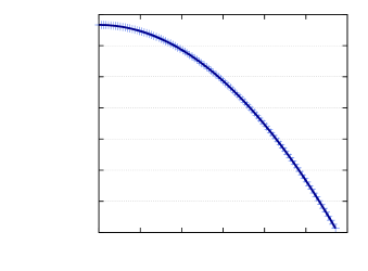
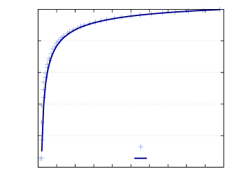
0.00×1000.00superscript1000.00\times 10^{0}5.00×1065.00superscript1065.00\times 10^{-6}1.00×1051.00superscript1051.00\times 10^{-5}1.50×1051.50superscript1051.50\times 10^{-5}2.00×1052.00superscript1052.00\times 10^{-5}2.50×1052.50superscript1052.50\times 10^{-5}3.00×1053.00superscript1053.00\times 10^{-5}3.50×1053.50superscript1053.50\times 10^{-5}0.0000.0000.0000.0010.0010.0010.0020.0020.0020.0030.0030.0030.0040.0040.0040.0050.0050.0050.0060.0060.006

R/rmax𝑅subscript𝑟𝑚𝑎𝑥R/r_{max}

ρ˙initsubscript˙𝜌𝑖𝑛𝑖𝑡\dot{\rho}_{init}R/rmax=0.9999765(ρ˙init)2𝑅subscript𝑟𝑚𝑎𝑥0.9999765superscriptsubscript˙𝜌𝑖𝑛𝑖𝑡2R/r_{max}\,=\,-0.9999765\,(\dot{\rho}_{init})^{2}+3.333×1053.333superscript105{}+3.333\times 10^{-5}RMS of residuals= 8.367×10¹¹RMS of residuals8.367superscript1011\text{RMS of residuals}\,=\,8.367\times 10^{-11}Refer to caption
Figure 33: A plot of R/rmax𝑅subscript𝑟𝑚𝑎𝑥R/r_{max} versus ρ˙initsubscript˙𝜌𝑖𝑛𝑖𝑡\dot{\rho}_{init} for rinit=3×10⁴Rsubscript𝑟𝑖𝑛𝑖𝑡3superscript104𝑅r_{init}=3\times 10^{4}\,R. A quadratic regression has been performed and the corresponding equation shown. The simulation’s block parameters were R=1𝑅1R=1, Δt=10ΔrΔ𝑡10Δ𝑟\Delta t=10\Delta r, Δr=R/10Δ𝑟𝑅10\Delta r=R/10, and Δϕ=2π/(3×107)Δitalic-ϕ2𝜋3superscript107\Delta\phi=2\pi/(3\times 10^{7}).
1.11.1-1.10.90.9-0.90.70.7-0.70.50.5-0.50.30.3-0.30.10.1-0.100101010202020303030404040505050606060707070808080909090100100100

ρ˙˙𝜌\dot{\rho}

r/R𝑟𝑅r/RRefer to captionsimulated velocityuρsuperscript𝑢𝜌u^{\rho}
Figure 34: A plot of ρ~˙˙~𝜌\dot{\tilde{\rho}} versus r/R𝑟𝑅r/R comparing a simulated particle velocity with uρsuperscript𝑢𝜌u^{\rho}. The simulation began at rinit=3×10⁴Rsubscript𝑟𝑖𝑛𝑖𝑡3superscript104𝑅r_{init}=3\times 10^{4}\,R, but only data points from r=2R𝑟2𝑅r=2\,R to 100R100𝑅100\,R are shown. The simulated velocity is always greater than or equal to uρsuperscript𝑢𝜌u^{\rho}. The simulation’s block parameters were R=1𝑅1R=1, Δt=Δr=RΔ𝑡Δ𝑟𝑅\Delta t=\Delta r=R, and Δϕ=2π/(3×107)Δitalic-ϕ2𝜋3superscript107\Delta\phi=2\pi/(3\times 10^{7}).

The discrepancy between ρ~˙˙~𝜌\dot{\tilde{\rho}} and uρsuperscript𝑢𝜌u^{\rho} can be understood by considering the manner by which particles are deflected in the Regge model. Suppose a particle enters a Regge block of radius risubscript𝑟𝑖r_{i} by the ρisubscript𝜌𝑖-\rho_{i} face and travels at the escape velocity as given by (44). If the particle then enters the next block by the ρi+1subscript𝜌𝑖1-\rho_{i+1} face as well, it will have undergone no deflection and hence continue having the same velocity as at risubscript𝑟𝑖r_{i}. However, (44) indicates that the escape velocity at ri+1subscript𝑟𝑖1r_{i+1} should be smaller than that at risubscript𝑟𝑖r_{i}, and hence we see the beginning of a discrepancy. If the particle passes through a sizeable number of ρ𝜌\rho faces in succession, it would accumulate a significant discrepancy such that the particle’s velocity would be noticeably larger than the escape velocity for its radius. This explains why the graphs for simulated particles in Fig. 32 are always smaller than the graph for uρsuperscript𝑢𝜌u^{\rho}. Only when the particle crosses a τ𝜏\tau surface does it undergo a change in velocity, but this change may not be enough to overcome the discrepancy already accumulated. By a similar argument, we expect the radial velocity of a radially in-going particle to decrease less quickly than uρsuperscript𝑢𝜌u^{\rho} in (44), because if the particle crosses a +ρ𝜌+\rho face with the correct escape velocity, it will cross the neighbouring +ρ𝜌+\rho face with the same unchanged velocity, which would be less negative than uρsuperscript𝑢𝜌u^{\rho} for the same radius; and indeed, this is what we see in Fig. 34. By improving the resolution of our Regge model, we slow the growth rate of the discrepancy, as we saw in Fig. 32, because our model becomes a better approximation to the underlying continuum Schwarzschild space-time and its geodesics therefore become more similar to those in the continuum space-time.

Thus combined with our analytic arguments provided at the end of Section VI, we conclude that (44) gives the correct velocity as a function of r𝑟r for particles following radial time-like geodesics.

Appendix C Radial lengths of Schwarzschild Regge blocks

In our simulations of the flat and open universes, our Regge blocks’ radial lengths were not constant but were increased as the blocks were further away from the Schwarschild-cell centre. This decision was motivated by the fact that the underlying space-time being approximated becomes increasingly flat. We therefore attempted to maintain higher resolution while the curvature was high but then decrease the resolution with minimal impact on accuracy as the curvature decreased. This technique allowed us to perform larger-scale simulations within more attainable computation times. We now describe our method for specifying the block’s radial length.

In Schwarzschild space-time, the radial distance between radius ri>2msubscript𝑟𝑖2𝑚r_{i}>2m and some arbitrary r>ri𝑟subscript𝑟𝑖r>r_{i} is given by

d(r)=[x12mx2mln(x2mx2m1)]x=rir.𝑑𝑟subscriptsuperscriptdelimited-[]𝑥12𝑚𝑥2𝑚𝑥2𝑚𝑥2𝑚1𝑟𝑥subscript𝑟𝑖d(r)=\left[x\sqrt{1\!-\!\frac{2m}{x}}-2m\ln\left(\!\sqrt{\frac{x}{2m}}\!-\!\sqrt{\frac{x}{2m}\!-\!1}\;\right)\!\right]^{r}_{x\,=\,r_{i}}. (57)

When r=ri+1𝑟subscript𝑟𝑖1r=r_{i+1}, this is identical to (37). Distances along ‘radial edges’ of Regge blocks approximate radial distances in Schwarzschild space-time by linearly interpolating d(r)𝑑𝑟d(r) between risubscript𝑟𝑖r_{i} and ri+1subscript𝑟𝑖1r_{i+1}, as shown in Fig. 35. Since d(r)𝑑𝑟d(r) is convex, the interpolation will always underestimate the true distance, and the error ε𝜀\varepsilon of the approximation is given by ε=max[d(r)lin(r)]𝜀𝑑𝑟lin𝑟\varepsilon=\max\left[d(r)-\mathrm{lin}(r)\right], where lin(r)lin𝑟\mathrm{lin}(r) denotes the interpolating function.

radialdistance𝑟𝑎𝑑𝑖𝑎𝑙𝑑𝑖𝑠𝑡𝑎𝑛𝑐𝑒radial\ distance

r𝑟rRefer to captionSchwarzschild space-timeRegge block interpolation
Figure 35: The Regge block interpolation intersects the Schwarzschild graph at r=ri𝑟subscript𝑟𝑖r=r_{i} and r=ri+1𝑟subscript𝑟𝑖1r=r_{i+1}, where ri<ri+1subscript𝑟𝑖subscript𝑟𝑖1r_{i}<r_{i+1} and where risubscript𝑟𝑖r_{i} corresponds to the origin of the graph; it interpolates the radial distance for only those values of r𝑟r lying between these two points of intersection. Since the Schwarzschild distance function is convex, the interpolation will always underestimate the distance in this regime.

Our goal is as follows. Given some error-tolerance εtolsubscript𝜀𝑡𝑜𝑙\varepsilon_{tol}, we want our blocks to be as long as possible in the radial direction while still satisfying εεtol𝜀subscript𝜀𝑡𝑜𝑙\varepsilon\leq\varepsilon_{tol}. If we enter a new block from its left or right face, then we would need to re-calculate the block’s radial length h=ri+1risubscript𝑟𝑖1subscript𝑟𝑖h=r_{i+1}-r_{i} in accordance with our goal. It will always be the case that we know one of risubscript𝑟𝑖r_{i} or ri+1subscript𝑟𝑖1r_{i+1} depending on which face we entered by, and we would need to deduce the other quantity. However our computation must give consistent results for hh regardless of which quantity we used. In our particular implementation, we have also chosen to impose the constraint that hh must be some integer units of a minimal interval Δr0Δsubscript𝑟0\Delta r_{0}, a parameter which we can freely specify.

The most natural approach would be to solve d(r)=lin(r)superscript𝑑𝑟superscriptlin𝑟d^{\prime}(r)=\mathrm{lin}^{\prime}(r), which maximises d(r)lin(r)𝑑𝑟lin𝑟d(r)-\mathrm{lin}(r), to obtain r=rmax𝑟subscript𝑟𝑚𝑎𝑥r=r_{max}, the point at which the error is greatest. Also through its dependence on lin(r)lin𝑟\mathrm{lin}(r), rmaxsubscript𝑟𝑚𝑎𝑥r_{max} would be a function of hh. We would then set ε=εtol𝜀subscript𝜀𝑡𝑜𝑙\varepsilon=\varepsilon_{tol} and solve d(rmax)lin(rmax)=εtol𝑑subscript𝑟𝑚𝑎𝑥linsubscript𝑟𝑚𝑎𝑥subscript𝜀𝑡𝑜𝑙d(r_{max})-\mathrm{lin}(r_{max})=\varepsilon_{tol} for hh. However, this second equation can only be solved numerically, and from a programming point of view, it was easier to implement a different approach instead.

We note that for r>ri𝑟subscript𝑟𝑖r>r_{i}, the functions d(r)𝑑𝑟d(r) and lin(r)lin𝑟\mathrm{lin}(r) are bounded from above by

d+(r)=riri1(rri)+d(ri),superscript𝑑𝑟subscript𝑟𝑖subscript𝑟𝑖1𝑟subscript𝑟𝑖𝑑subscript𝑟𝑖d^{+}(r)=\sqrt{\frac{r_{i}}{r_{i}-1}}(r-r_{i})+d(r_{i}), (58)

since this is just the equation of the tangent to d(r)𝑑𝑟d(r) at risubscript𝑟𝑖r_{i}. And also, for r>ri𝑟subscript𝑟𝑖r>r_{i}, the two functions are bounded from below by

d(r)=(rri)+d(ri);superscript𝑑𝑟𝑟subscript𝑟𝑖𝑑subscript𝑟𝑖d^{-}(r)=(r-r_{i})+d(r_{i}); (59)

this follows because the gradient of d(r)𝑑𝑟d(r) goes asymptotically to unity from above as r𝑟r\to\infty, which means d(r)𝑑𝑟d(r) will always increase more quickly than d(r)superscript𝑑𝑟d^{-}(r). Therefore, after the two functions have intercepted at r=ri𝑟subscript𝑟𝑖r=r_{i}, d(r)𝑑𝑟d(r) will always be strictly greater than d(r)superscript𝑑𝑟d^{-}(r). The function lin(r)lin𝑟\mathrm{lin}(r) also intercepts both d(r)𝑑𝑟d(r) and d(r)superscript𝑑𝑟d^{-}(r) at r=ri𝑟subscript𝑟𝑖r=r_{i}. But it intercepts d(r)𝑑𝑟d(r) again at ri+1>risubscript𝑟𝑖1subscript𝑟𝑖r_{i+1}>r_{i}, a point where d(r)>d(r)𝑑𝑟superscript𝑑𝑟d(r)>d^{-}(r). Because lin(r)lin𝑟\mathrm{lin}(r) is a linear function, this interception at ri+1subscript𝑟𝑖1r_{i+1} implies that lin(r)lin𝑟\mathrm{lin}(r) must have a greater gradient than d(r)superscript𝑑𝑟d^{-}(r), and therefore lin(r)lin𝑟\mathrm{lin}(r) must also be strictly greater than d(r)superscript𝑑𝑟d^{-}(r) in the region r>ri𝑟subscript𝑟𝑖r>r_{i}.

Thus we can bound our error by

εmax[d+(r)d(r)]=d+(ri+1)d(ri+1).𝜀superscript𝑑𝑟superscript𝑑𝑟superscript𝑑subscript𝑟𝑖1superscript𝑑subscript𝑟𝑖1\varepsilon\leq\max\left[d^{+}(r)-d^{-}(r)\right]=d^{+}(r_{i+1})-d^{-}(r_{i+1}).

We shall therefore require that

εtold+(ri+1)d(ri+1),subscript𝜀𝑡𝑜𝑙superscript𝑑subscript𝑟𝑖1superscript𝑑subscript𝑟𝑖1\varepsilon_{tol}\geq d^{+}(r_{i+1})-d^{-}(r_{i+1}),

and solve for ri+1subscript𝑟𝑖1r_{i+1} from this equation; this yields the solution

h=εtolri/(ri1)1.subscript𝜀𝑡𝑜𝑙subscript𝑟𝑖subscript𝑟𝑖11h=\frac{\varepsilon_{tol}}{\sqrt{r_{i}/(r_{i}-1)}-1}.

To get hh as a function of ri+1subscript𝑟𝑖1r_{i+1} instead, we set risubscript𝑟𝑖r_{i} to be ri=ri+1hsubscript𝑟𝑖subscript𝑟𝑖1r_{i}=r_{i+1}-h and solve for hh in the preceding equation; this yields

h=εtol2(2εtol1){2ri+1+εtol2+[4ri+1(ri+11εtol)+εtol(4+εtol)]1/2}.subscript𝜀𝑡𝑜𝑙22subscript𝜀𝑡𝑜𝑙12subscript𝑟𝑖1subscript𝜀𝑡𝑜𝑙2superscriptdelimited-[]4subscript𝑟𝑖1subscript𝑟𝑖11subscript𝜀𝑡𝑜𝑙subscript𝜀𝑡𝑜𝑙4subscript𝜀𝑡𝑜𝑙12h=\frac{\varepsilon_{tol}}{2(2\varepsilon_{tol}-1)}\left\{2r_{i+1}+\varepsilon_{tol}-2\vphantom{\Big{]}^{1/2}}+\Big{[}4r_{i+1}(r_{i+1}-1-\varepsilon_{tol})+\varepsilon_{tol}(4+\varepsilon_{tol})\Big{]}^{1/2}\right\}.

As mentioned above, we want hh to satisfy h=nΔr0𝑛Δsubscript𝑟0h=n\,\Delta r_{0} for some integer n𝑛n. Therefore our actual hh is obtained by taking n𝑛n to be

n=εtolΔr0(ri/(ri1)1)𝑛subscript𝜀𝑡𝑜𝑙Δsubscript𝑟0subscript𝑟𝑖subscript𝑟𝑖11n=\left\lfloor\frac{\varepsilon_{tol}}{\Delta r_{0}\left(\sqrt{r_{i}/(r_{i}-1)}-1\right)}\right\rfloor (60)

or

n=εtol2Δr0(2εtol1){2ri+1+εtol2+[4ri+1(ri+11εtol)+εtol(4+εtol)]1/2}.𝑛subscript𝜀𝑡𝑜𝑙2Δsubscript𝑟02subscript𝜀𝑡𝑜𝑙12subscript𝑟𝑖1subscript𝜀𝑡𝑜𝑙2superscriptdelimited-[]4subscript𝑟𝑖1subscript𝑟𝑖11subscript𝜀𝑡𝑜𝑙subscript𝜀𝑡𝑜𝑙4subscript𝜀𝑡𝑜𝑙12\begin{split}n=\left\lfloor\frac{\varepsilon_{tol}}{2\Delta r_{0}(2\varepsilon_{tol}-1)}\right.&\left\{2r_{i+1}+\varepsilon_{tol}-2\vphantom{\Big{]}^{1/2}}\right.\\ &\hphantom{\{}{}+\Big{[}4r_{i+1}(r_{i+1}-1-\varepsilon_{tol})\\ &\left.\left.\hphantom{(2r}{}+\varepsilon_{tol}(4+\varepsilon_{tol})\Big{]}^{1/2}\right\}\right\rfloor.\end{split} (61)

as appropriate, where x𝑥\lfloor x\rfloor gives the greatest integer less than or equal to x𝑥x, and then substituting this n𝑛n into h=nΔr0𝑛Δsubscript𝑟0h=n\,\Delta r_{0}.

Finally, we want to ensure that our algorithm would give the same hh regardless of whether it used risubscript𝑟𝑖r_{i} or ri+1subscript𝑟𝑖1r_{i+1}. To satisfy this requirement, whenever the program calculated ri+1subscript𝑟𝑖1r_{i+1} from risubscript𝑟𝑖r_{i}, it would check to see if it could recover the same hh using the new value for ri+1subscript𝑟𝑖1r_{i+1}. If not, then it would decrement hh by one unit of Δr0Δsubscript𝑟0\Delta r_{0} and check again, and it would continue decrementing until obtaining agreement. The program can only decrement if the error is to remain within tolerance. We had also required that hh be at least Δr0Δsubscript𝑟0\Delta r_{0}; thus the decrementing would stop if hh reached this length.

Appendix D Boundary conditions for Schwarzschild-cells of unequal masses

An observer sitting at the interface of two cell boundaries must observe the same physics regardless of which co-ordinate system the observer uses. In particular, the following two conditions must be satisfied:

  1. 1)

    the observer must measure the same proper time regardless of which cell’s metric is used;

  2. 2)

    and the observer must measure the same spatial distances locally along the boundary regardless of which cell’s metric is used.

However if the cells in the lattice are no longer identical, we would no longer have the same lattice symmetries as before. In particular, the exact location of the boundary between two unequal cells becomes less transparent, as it is no longer equidistant to the two cell centres. Recall that in the perfectly symmetric lattice, a test particle sitting on the boundary between two cells would by symmetry always remain at the boundary and yet fall simultaneously towards both cell centres. Although the symmetry is no longer present when the two cells are no longer identical, we shall still assume that test particles at the boundary fall simultaneously to both centres. This condition defines the location of the cell boundary for us: it is effectively defined to be where the two cells’ gravitational influences are equal. On one side of the boundary, the gravitational influence of one mass dominates, and we approximate the space-time by a Schwarzschild space-time centred on that mass. On the other side, the other mass dominates, and we approximate the space-time with a Schwarzschild space-time centred on that mass. Once again, we can understand this simultaneous free-fall of the boundary towards the two centres as actually the motion of the two masses towards each other under their mutual attraction. This mutual attraction gives rise to the expansion and contraction of the lattice itself, which manifests as the expansion and contraction of the cell boundary. Given this definition and our two boundary conditions, we can now derive a set of constraints that Ebsubscript𝐸𝑏E_{b} and the cell radius rbsubscript𝑟𝑏r_{b} must satisfy.

Local spatial distances along the boundary are given by

rbdΩ.subscript𝑟𝑏𝑑Ωr_{b}\,d\Omega. (62)

Since by assumption, particles co-moving with the boundary follow radial geodesics, then this distance evolves as

drbdτdΩ.𝑑subscript𝑟𝑏𝑑𝜏𝑑Ω\frac{dr_{b}}{d\tau}\,d\Omega. (63)

By condition (2), we require that

rb1dΩ1=rb2dΩ2,subscript𝑟subscript𝑏1𝑑subscriptΩ1subscript𝑟subscript𝑏2𝑑subscriptΩ2r_{b_{1}}\,d\Omega_{1}=r_{b_{2}}\,d\Omega_{2}, (64)

where the numerical subscripts refer to cells 1 and 2; combined with condition (1), we additionally require that

drb1dτdΩ1=drb2dτdΩ2,𝑑subscript𝑟subscript𝑏1𝑑𝜏𝑑subscriptΩ1𝑑subscript𝑟subscript𝑏2𝑑𝜏𝑑subscriptΩ2\frac{dr_{b_{1}}}{d\tau}\,d\Omega_{1}=\frac{dr_{b_{2}}}{d\tau}\,d\Omega_{2}, (65)

since dτ1=dτ2=dτ𝑑subscript𝜏1𝑑subscript𝜏2𝑑𝜏d\tau_{1}=d\tau_{2}=d\tau. Combining these two conditions, we obtain

1rb1drb1dτ=1rb2drb2dτ,1subscript𝑟subscript𝑏1𝑑subscript𝑟subscript𝑏1𝑑𝜏1subscript𝑟subscript𝑏2𝑑subscript𝑟subscript𝑏2𝑑𝜏\frac{1}{r_{b_{1}}}\frac{dr_{b_{1}}}{d\tau}=\frac{1}{r_{b_{2}}}\frac{dr_{b_{2}}}{d\tau}, (66)

and using (5), we can express this equivalently as

1rb1Eb11+2m1rb1=1rb2Eb21+2m2rb2.1subscript𝑟subscript𝑏1subscript𝐸subscript𝑏112subscript𝑚1subscript𝑟subscript𝑏11subscript𝑟subscript𝑏2subscript𝐸subscript𝑏212subscript𝑚2subscript𝑟subscript𝑏2\frac{1}{r_{b_{1}}}\sqrt{E_{b_{1}}-1+\frac{2m_{1}}{r_{b_{1}}}}=\frac{1}{r_{b_{2}}}\sqrt{E_{b_{2}}-1+\frac{2m_{2}}{r_{b_{2}}}}. (67)

By condition (1), we require that Δτ1=Δτ2Δsubscript𝜏1Δsubscript𝜏2\Delta\tau_{1}=\Delta\tau_{2}. Recall that the proper time of a freely falling particle is given by equations (6) to (15). However, from the form of equations (6) to (6), it is clear that we cannot satisfy this condition unless both cells are of the same type, that is, both cells are open, flat, or closed. This constrains the cases we need to consider to just three, and we shall consider each in turn.

If Eb=1subscript𝐸𝑏1E_{b}=1 for both cells, then (6) and (15) imply that

Δτ1Δsubscript𝜏1\displaystyle\Delta\tau_{1} =Δτ2absentΔsubscript𝜏2\displaystyle=\Delta\tau_{2}
2312m1rb13/2τ02312subscript𝑚1superscriptsubscript𝑟subscript𝑏132subscript𝜏0\displaystyle\frac{2}{3}\frac{1}{\sqrt{2m_{1}}}\,r_{b_{1}}^{3/2}-\tau_{0} =2312m2rb23/2τ0,absent2312subscript𝑚2superscriptsubscript𝑟subscript𝑏232subscript𝜏0\displaystyle=\frac{2}{3}\frac{1}{\sqrt{2m_{2}}}\,r_{b_{2}}^{3/2}-\tau_{0},

where τ0subscript𝜏0\tau_{0} is a constant of integration. From this, we obtain the relation

rb2=(m2m1)1/3rb1.subscript𝑟subscript𝑏2superscriptsubscript𝑚2subscript𝑚113subscript𝑟subscript𝑏1r_{b_{2}}=\left(\frac{m_{2}}{m_{1}}\right)^{1/3}\,r_{b_{1}}. (68)

It can be checked that this relation also satisfies (67) and hence condition (2) as well.

If Eb<1subscript𝐸𝑏1E_{b}<1 for both cells, then (6) and (15) imply that

2m1(1Eb1)3/2[1Eb12m1rb111Eb12m1rb1+cos11Eb12m1rb1]τ02subscript𝑚1superscript1subscript𝐸subscript𝑏132delimited-[]1subscript𝐸subscript𝑏12subscript𝑚1subscript𝑟subscript𝑏111subscript𝐸subscript𝑏12subscript𝑚1subscript𝑟subscript𝑏1superscript11subscript𝐸subscript𝑏12subscript𝑚1subscript𝑟subscript𝑏1subscript𝜏0\displaystyle\frac{2m_{1}}{\left(1-E_{b_{1}}\right)^{3/2}}\left[\sqrt{\frac{1-E_{b_{1}}}{2m_{1}}r_{b_{1}}}\sqrt{1-\frac{1-E_{b_{1}}}{2m_{1}}r_{b_{1}}}+\cos^{-1}\sqrt{\frac{1-E_{b_{1}}}{2m_{1}}r_{b_{1}}}\right]-\tau_{0}
=2m2(1Eb2)3/2[1Eb22m2rb211Eb22m2rb2+cos11Eb22m2rb2]τ0.absent2subscript𝑚2superscript1subscript𝐸subscript𝑏232delimited-[]1subscript𝐸subscript𝑏22subscript𝑚2subscript𝑟subscript𝑏211subscript𝐸subscript𝑏22subscript𝑚2subscript𝑟subscript𝑏2superscript11subscript𝐸subscript𝑏22subscript𝑚2subscript𝑟subscript𝑏2subscript𝜏0\displaystyle\qquad\qquad=\frac{2m_{2}}{\left(1-E_{b_{2}}\right)^{3/2}}\left[\sqrt{\frac{1-E_{b_{2}}}{2m_{2}}r_{b_{2}}}\sqrt{1-\frac{1-E_{b_{2}}}{2m_{2}}r_{b_{2}}}+\cos^{-1}\sqrt{\frac{1-E_{b_{2}}}{2m_{2}}r_{b_{2}}}\right]-\tau_{0}.

The two sides of this equation can be made equal if we simultaneously equated

1Eb12m1rb1=1subscript𝐸subscript𝑏12subscript𝑚1subscript𝑟subscript𝑏1absent\displaystyle\frac{1-E_{b_{1}}}{2m_{1}}r_{b_{1}}={} 1Eb22m2rb21subscript𝐸subscript𝑏22subscript𝑚2subscript𝑟subscript𝑏2\displaystyle\frac{1-E_{b_{2}}}{2m_{2}}r_{b_{2}}
and
2m1(1Eb1)3/2=2subscript𝑚1superscript1subscript𝐸subscript𝑏132absent\displaystyle\frac{2m_{1}}{\left(1-E_{b_{1}}\right)^{3/2}}={} 2m2(1Eb2)3/2.2subscript𝑚2superscript1subscript𝐸subscript𝑏232\displaystyle\frac{2m_{2}}{\left(1-E_{b_{2}}\right)^{3/2}}.

The second equation leads to the constraint

(Eb21)=(m2m1)2/3(Eb11),subscript𝐸subscript𝑏21superscriptsubscript𝑚2subscript𝑚123subscript𝐸subscript𝑏11\left(E_{b_{2}}-1\right)=\left(\frac{m_{2}}{m_{1}}\right)^{2/3}\,\left(E_{b_{1}}-1\right), (69)

and if we substitute this into the first equation, we recover (68). Again, it can be checked that (68) and (69) combined satisfy (67) and hence condition (2) as well.

Finally if Eb>1subscript𝐸𝑏1E_{b}>1, then (6) and (15) imply that

2m1(Eb11)3/2[Eb112m1rb11+Eb112m1rb1sinh1Eb112m1rb1]τ02subscript𝑚1superscriptsubscript𝐸subscript𝑏1132delimited-[]subscript𝐸subscript𝑏112subscript𝑚1subscript𝑟subscript𝑏11subscript𝐸subscript𝑏112subscript𝑚1subscript𝑟subscript𝑏1superscript1subscript𝐸subscript𝑏112subscript𝑚1subscript𝑟subscript𝑏1subscript𝜏0\displaystyle\frac{2m_{1}}{\left(E_{b_{1}}-1\right)^{3/2}}\left[\sqrt{\frac{E_{b_{1}}-1}{2m_{1}}r_{b_{1}}}\sqrt{1+\frac{E_{b_{1}}-1}{2m_{1}}r_{b_{1}}}-\sinh^{-1}\sqrt{\frac{E_{b_{1}}-1}{2m_{1}}r_{b_{1}}}\right]-\tau_{0}
=2m2(Eb21)3/2[Eb212m2rb21+Eb212m2rb2sinh1Eb212m2rb2]τ0.absent2subscript𝑚2superscriptsubscript𝐸subscript𝑏2132delimited-[]subscript𝐸subscript𝑏212subscript𝑚2subscript𝑟subscript𝑏21subscript𝐸subscript𝑏212subscript𝑚2subscript𝑟subscript𝑏2superscript1subscript𝐸subscript𝑏212subscript𝑚2subscript𝑟subscript𝑏2subscript𝜏0\displaystyle\qquad\qquad=\frac{2m_{2}}{\left(E_{b_{2}}-1\right)^{3/2}}\left[\sqrt{\frac{E_{b_{2}}-1}{2m_{2}}r_{b_{2}}}\sqrt{1+\frac{E_{b_{2}}-1}{2m_{2}}r_{b_{2}}}-\sinh^{-1}\sqrt{\frac{E_{b_{2}}-1}{2m_{2}}r_{b_{2}}}\right]-\tau_{0}.

As with the Eb<1subscript𝐸𝑏1E_{b}<1 case, the two sides of this equation can be made equal if we simultaneously equated

Eb112m1rb1=subscript𝐸subscript𝑏112subscript𝑚1subscript𝑟subscript𝑏1absent\displaystyle\frac{E_{b_{1}}-1}{2m_{1}}r_{b_{1}}={} Eb212m2rb2subscript𝐸subscript𝑏212subscript𝑚2subscript𝑟subscript𝑏2\displaystyle\frac{E_{b_{2}}-1}{2m_{2}}r_{b_{2}}
and
2m1(Eb11)3/2=2subscript𝑚1superscriptsubscript𝐸subscript𝑏1132absent\displaystyle\frac{2m_{1}}{\left(E_{b_{1}}-1\right)^{3/2}}={} 2m2(Eb21)3/2.2subscript𝑚2superscriptsubscript𝐸subscript𝑏2132\displaystyle\frac{2m_{2}}{\left(E_{b_{2}}-1\right)^{3/2}}.

This clearly leads to the same constraints as in the Eb<1subscript𝐸𝑏1E_{b}<1 case.

We therefore find that for all cases, two neighbouring cells must satisfy constraints (68) and (69) at the boundary.181818The author wishes to acknowledge that constraints (68) and (69) were actually first derived by Ruth Williams in an unpublished calculation, where she derived the boundary conditions using the Israeli junction conditions instead. Equating the two metrics on the boundary gave the condition drb1/dτ1=drb2/dτ2𝑑subscript𝑟subscript𝑏1𝑑subscript𝜏1𝑑subscript𝑟subscript𝑏2𝑑subscript𝜏2dr_{b_{1}}/d\tau_{1}=dr_{b_{2}}/d\tau_{2}, and equating TrκTr𝜅\operatorname{Tr}{\kappa}, where κ𝜅\kappa is the extrinsic curvature, gave condition (66). And when m1=m2subscript𝑚1subscript𝑚2m_{1}=m_{2}, we recover Eb1=Eb2subscript𝐸subscript𝑏1subscript𝐸subscript𝑏2E_{b_{1}}=E_{b_{2}} and rb1=rb2subscript𝑟subscript𝑏1subscript𝑟subscript𝑏2r_{b_{1}}=r_{b_{2}}.

References

  • Ellis and Buchert (2005) G. F. R. Ellis and T. Buchert, Phys. Lett. A 347, 38 (2005), arXiv:gr-qc/0506106 .
  • Ellis (2011) G. F. R. Ellis, Class. Quantum Grav. 28, 164001 (2011), arXiv:1103.2335 .
  • Clarkson et al. (2011) C. Clarkson, G. F. R. Ellis, J. Larena,  and O. Umeh, Rept. Prog. Phys. 74, 112901 (2011), arXiv:1109.2314 .
  • Kolb et al. (2006) E. W. Kolb, S. Matarrese,  and A. Riotto, New J. Phys. 8, 322 (2006), arXiv:astro-ph/0506534 .
  • Clarkson and Maartens (2010) C. Clarkson and R. Maartens, Class. Quantum Grav. 27, 124008 (2010), arXiv:1005.2165 .
  • Clarkson and Umeh (2011) C. Clarkson and O. Umeh, Class. Quantum Grav. 28, 164010 (2011), arXiv:1105.1886 .
  • Mustapha et al. (1997) N. Mustapha, C. Hellaby,  and G. F. R. Ellis, Mon. Not. R. Astron. Soc. 292, 817 (1997), arXiv:gr-qc/9808079 .
  • Célérier and Schneider (1998) M.-N. Célérier and J. Schneider, Phys. Lett. A 249, 37 (1998), arXiv:astro-ph/9809134 .
  • Tomita (2000a) K. Tomita, Astrophys. J. 529, 26 (2000a), arXiv:astro-ph/9905278 .
  • Tomita (2000b) K. Tomita, Astrophys. J. 529, 38 (2000b), arXiv:astro-ph/9906027 .
  • Alnes et al. (2006) H. Alnes, M. Amarzguioui,  and Ø. Grøn, Phys. Rev. D 73, 083519 (2006), arXiv:astro-ph/0512006 .
  • Moffat (2006) J. W. Moffat, J. Cosmol. Astropart. Phys. 06, 001 (2006), arXiv:astro-ph/0505326 .
  • Mansouri (2006) R. Mansouri, “Structured FRW universe leads to acceleration: a non-perturbative approach,”  (2006), arXiv:astro-ph/0512605 .
  • Garcia-Bellido and Haugbølle (2008) J. Garcia-Bellido and T. Haugbølle, J. Cosmol. Astropart. Phys. 08, 003 (2008), arXiv:0802.1523 .
  • Clifton et al. (2008) T. Clifton, P. G. Ferreira,  and K. Land, Phys. Rev. Lett. 101, 131302 (2008)arXiv:0807.1443 .
  • Chuang et al. (2008) C.-H. Chuang, J.-A. Gu,  and W.-Y. P. Hwang, Class. Quantum Grav. 25, 175001 (2008), arXiv:astro-ph/0512651 .
  • Alexander et al. (2009) S. Alexander, T. Biswas, A. Notari,  and D. Vaid, J. Cosmol. Astropart. Phys. 09, 025 (2009), arXiv:0712.0370 .
  • Bolejko and Wyithe (2009) K. Bolejko and J. S. B. Wyithe, J. Cosmol. Astropart. Phys. 09, 020 (2009), arXiv:0807.2891 .
  • February et al. (2010) S. February, J. Larena, M. Smith,  and C. Clarkson, Mon. Not. R. Astron. Soc. 405, 2231 (2010), arXiv:0909.1479 .
  • Einstein and Straus (1945) A. Einstein and E. G. Straus, Rev. Mod. Phys. 17, 120 (1945).
  • Einstein and Straus (1946) A. Einstein and E. G. Straus, Rev. Mod. Phys. 18, 148 (1946).
  • Kantowski (1969) R. Kantowski, Astrophys. J. 155, 89 (1969).
  • Biswas and Notari (2008) T. Biswas and A. Notari, J. Cosmol. Astropart. Phys. 08, 021 (2008), arXiv:astro-ph/0702555 .
  • Marra et al. (2007) V. Marra, E. W. Kolb, S. Matarrese,  and A. Riotto, Phys. Rev. D 76, 123004 (2007), arXiv:0708.3622 .
  • Brouzakis et al. (2008) N. Brouzakis, N. Tetradis,  and E. Tzavara, J. Cosmol. Astropart. Phys. 08, 008 (2008), arXiv:astro-ph/0703586 .
  • Marra et al. (2008) V. Marra, E. W. Kolb,  and S. Matarrese, Phys. Rev. D 77, 023003 (2008), arXiv:0710.5505 .
  • Clifton and Zuntz (2009) T. Clifton and J. Zuntz, Mon. Not. R. Astron. Soc. 400, 2185 (2009), arXiv:0902.0726 .
  • Wheeler (1983) J. A. Wheeler, Found. Phys. 13, 161 (1983).
  • Clifton et al. (2012a) T. Clifton, K. Rosquist,  and R. Tavakol, Phys. Rev. D 86, 043506 (2012a), arXiv:1203.6478 .
  • Korzyński (2014) M. Korzyński, Class. Quantum Grav. 31, 085002 (2014), arXiv:1312.0494 .
  • Bentivegna and Korzyński (2012) E. Bentivegna and M. Korzyński, Class. Quantum Grav. 29, 165007 (2012), arXiv:1204.3568 .
  • Clifton et al. (2013) T. Clifton, D. Gregoris, K. Rosquist,  and R. Tavakol, J. Cosmol. Astropart. Phys. 13, 010 (2013), arXiv:1309.2876 .
  • Clifton et al. (2014) T. Clifton, D. Gregoris,  and K. Rosquist, Class. Quantum Grav. 31, 105012 (2014), arXiv:1402.3201 .
  • Bruneton and Larena (2012) J.-P. Bruneton and J. Larena, Class. Quantum Grav. 29, 155001 (2012), arXiv:1204.3433 .
  • Yoo et al. (2012) C.-M. Yoo, H. Abe, Y. Takamori,  and K.-i. Nakao, Phys. Rev. D 86, 044027 (2012), arXiv:1204.2411 .
  • Yoo et al. (2013) C.-M. Yoo, H. Okawa,  and K.-i. Nakao, Phys. Rev. Lett. 111, 161102 (2013), arXiv:1306.1389 .
  • Bentivegna and Korzyński (2013) E. Bentivegna and M. Korzyński, Class. Quantum Grav. 30, 235008 (2013), arXiv:1306.4055 .
  • Bruneton and Larena (2013) J.-P. Bruneton and J. Larena, Class. Quantum Grav. 30, 025002 (2013), arXiv:1208.1411 .
  • Lindquist and Wheeler (1957) R. W. Lindquist and J. A. Wheeler, Rev. Mod. Phys. 29, 432 (1957).
  • Lindquist and Wheeler (1959) R. W. Lindquist and J. A. Wheeler, Rev. Mod. Phys. 31, 839 (1959).
  • Wheeler (1964) J. A. Wheeler, in Relativity, Groups, and Topology, edited by C. DeWitt and B. S. DeWitt (Gordon and Breach Science Publishers, New York, 1964) pp. 315–520.
  • Clifton and Ferreira (2009a) T. Clifton and P. G. Ferreira, Phys. Rev. D 80, 103503 (2009a), arXiv:0907.4109 .
  • Clifton and Ferreira (2011) T. Clifton and P. G. Ferreira, Phys. Rev. D 84, 109902(E) (2011).
  • Clifton et al. (2012b) T. Clifton, P. G. Ferreira,  and K. O’Donnell, Phys. Rev. D 85, 023502 (2012b), arXiv:1110.3191 .
  • Williams and Ellis (1981) R. M. Williams and G. F. R. Ellis, Gen. Relativ. Gravit. 13, 361 (1981).
  • Williams and Ellis (1984) R. M. Williams and G. F. R. Ellis, Gen. Relativ. Gravit. 16, 1003 (1984).
  • Wigner and Seitz (1933) E. Wigner and F. Seitz, Phys. Rev. 43, 804 (1933).
  • Shockley (1937) W. Shockley, Phys. Rev. 52, 866 (1937).
  • von der Lage and Bethe (1947) F. C. von der Lage and H. A. Bethe, Phys. Rev. 71, 612 (1947).
  • Brewin and Gentle (2001) L. C. Brewin and A. P. Gentle, Class. Quantum Grav. 18, 517 (2001), arXiv:gr-qc/0006017 .
  • Sachs and Wolfe (1967) R. K. Sachs and A. M. Wolfe, Astrophys. J. 147, 73 (1967).
  • Rees and Sciama (1968) M. J. Rees and D. W. Sciama, Nature 217, 511 (1968).
  • Martínez-González et al. (1990) E. Martínez-González, J. L. Sanz,  and J. Silk, Astrophys. J. 355, L5 (1990).
  • Nishizawa (2014) A. J. Nishizawa, Prog. Theor. Exp. Phys. 2014, 06B110 (2014), arXiv:1404.5102 .
  • Crittenden and Turok (1996) R. G. Crittenden and N. Turok, Phys. Rev. Lett. 76, 575 (1996), arXiv:astro-ph/9510072 .
  • Boughn and Crittenden (2004) S. Boughn and R. Crittenden, Nature 427, 45 (2004), arXiv:astro-ph/0305001 .
  • Planck collaboration (2015) Planck collaboration, “Planck 2015 results. XXI. The integrated Sachs-Wolfe effect,”  (2015), arXiv:1502.01595 .
  • Clifton and Ferreira (2009b) T. Clifton and P. G. Ferreira, J. Cosmol. Astropart. Phys. 09, 026 (2009b), arXiv:0908.4488 .
  • Coxeter (1948) H. S. M. Coxeter, Regular Polytopes (Methuen and Company, Ltd, London, 1948).