Parity lifetime of bound states in a proximitized semiconductor nanowire

Quasiparticle excitations can compromise the performance of superconducting devices, causing high frequency dissipation, decoherence in Josephson qubits Lang:2003fk ; Aumentado:2004ij ; Martinis:2009bd ; DeVisser:2011bm ; Saira:2012ca ; Pop:2014gg , and braiding errors in proposed Majorana-based topological quantum computers Leijnse:2011dfa ; Rainis:2012uw ; Cheng:2012bu . Quasiparticle dynamics have been studied in detail in metallic superconductors Ferguson:2006hg ; Zgirski:2011wp ; Sun:2012gl ; Riste:2013il ; Maisi:2013cr but remain relatively unexplored in semiconductor-superconductor structures, which are now being intensely pursued in the context of topological superconductivity. To this end, we introduce a new physical system comprised of a gate-confined semiconductor nanowire with an epitaxially grown superconductor layer, yielding an isolated, proximitized nanowire segment. We identify Andreev-like bound states in the semiconductor via bias spectroscopy, determine the characteristic temperatures and magnetic fields for quasiparticle excitations, and extract a parity lifetime (poisoning time) of the bound state in the semiconductor exceeding 10 ms.

Semiconductor-superconductor hybrids have been investigated for many years Doh:2005wu ; Hofstetter:2009bm ; Pillet:2010ds ; DeFranceschi:2010tq ; Giazotto:2011jq , but recently have received renewed interest in the context of topological superconductivity, motivated by the realization that combining spin-orbit interaction, Zeeman splitting and proximity coupling to a conventional s-wave superconductor provides the necessary ingredients to create Majorana modes at the ends of a one-dimensional (1D) wire. Such modes are expected to show nonabelian statistics, allowing, in principle, topological encoding of quantum information Sau:2010cl ; Lutchyn:2010hp ; Oreg:2010gk among other interesting effects Padurariu:2010fr ; Leijnse:2013ba .

Transport experiments on semiconductor nanowires proximitized by a grounded superconductor have recently revealed characteristic features of Majorana modes Mourik:2012je ; Das:2012hi ; Deng:2012gn ; Churchill:2013cq . Semiconductor quantum dots with superconducting leads have also been explored experimentally Deacon:2010jna ; Lee:2012ft ; Lee:2013gj ; Chang:2013fo , and have been proposed as a basis for Majorana chains Sau:2012iu ; Leijnse:2012jf ; Fulga:2013dd . Here, we expand the geometries investigated in this context by creating an isolated semiconductor-supercondutor hybrid quantum dot (HQD) connected to normal leads. The device forms the basis of an isolated Majorana system with protected total parity, where both the semiconductor nanowire and the metallic superconductor are mesoscopic Fu:2010ho ; Hutzen:2012gg .

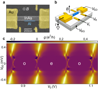
Figure 1: Nanowire-based hybrid quantum dot. a, Scanning electron micrograph of the reported device, consisting of an InAs nanowire (gray) with segment of epitaxial Al on two facets (blue) and Ti/Au contacts and side gates (yellow) on a doped silicon substrate. b, Device schematic and measurement setup, showing orientation of magnetic field, $B$. c, Differential conductance, $g$, as a function of effective gate voltage, $V_{\text{G}}$, and source-drain voltage, $V_{\text{SD}}$, at $B=0$. Even (e) and odd (o) occupied Coulomb valleys labeled.

The measured device consists of an InAs nanowire with epitaxial superconducting Al on two facets of the hexagonal wire, with Au ohmic contacts (Figs. 1a,b). Four devices showing similar behavior have been measured. The InAs nanowire was grown without stacking faults using molecular beam epitaxy with Al deposited in situ to ensure high-quality proximity effect Krogstrup:2015en ; Chang:2015kw . Differential conductance, $g$, was measured in a dilution refrigerator with base electron temperature $T\sim 50~{}\mathrm{mK}$ using standard ac lock-in techniques. Local side gates, patterned with electron beam lithography, and a global back gate were adjusted to form an Al-InAs HQD in the Coulomb blockade regime, with gate-controlled weak tunneling to the leads. The lower right gate, $V_{\mathrm{R}}$, was used to tune the occupation of the dot, with a linear compensation from the lower left gate, $V_{\mathrm{L}}$, to keep tunneling to the leads symmetric. We parameterize this with a single effective gate voltage, $V_{\mathrm{G}}$ (see Supplement).

Differential conductance as a function of $V_{\mathrm{G}}$ and source-drain bias, $V_{\mathrm{SD}}$, reveals a series of Coulomb diamonds, corresponding to incremental single-charge states of the HQD (Fig. 1c). While conductance features at high bias are essentially identical in each diamond, at low bias, $V_{\mathrm{SD}}<$ 0.2 mV, a distinctive even-odd pattern of left- and right-facing conductance features is observed. This results in an even-odd alternation of Coulomb blockade peak spacings at zero bias, similar to even-odd spacings seen in metallic superconductors Tuominen:1992ip ; Lafarge:1993vn . However, the parity-dependent reversing pattern of subgap features at nonzero bias has not been reported before, to our knowledge. The even-odd pattern indicates that a parity-sensitive bound state is being filled and emptied as electrons are added to the HQD.

Measured charging energy, $E_{C}=1.1~{}\mathrm{meV}$, and superconducting gap, $\Delta=180~{}\mathrm{\mu eV}$, satisfy the condition ($\Delta\ <\ E_{C}$) for single electron charging Averin:1992hy ; Matveev:1994fq . Differential conductance at low bias occurs in a series of narrow features symmetric about zero bias, suggesting transport through an Andreev-like bound state, with negative differential conductance (NDC) observed at the border of odd diamonds. NDC arises from slow quasiparticle escape, as discussed below, similar to current-blocking seen in metallic superconducting islands in the opposite regime, $\Delta>E_{C}$ Hekking:1993gc ; Hergenrother:1994ei .

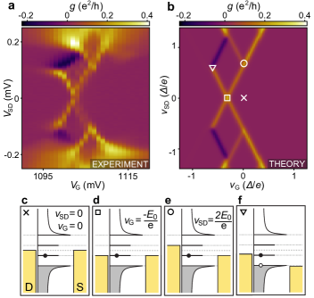
Figure 2: Subgap bias spectroscopy, experiment and model. a, Experimental differential conductance, $g$, as a function of gate voltage $V_{\mathrm{G}}$ and source-drain $V_{\mathrm{SD}}$, shows characteristic pattern including negative differential conductivity (NDC). b, Transport model of a. $v_{\text{G}}=\alpha V_{\mathrm{G}}$ up to an offset, where $\alpha$ is the gate lever arm. Axis units are $\Delta/e=180~{}\mathrm{\mu V}$, where $\Delta$ is the superconducting gap. See text for model parameters. c, Source and drain (gold) chemical potentials align with the middle of the gap in the HQD density of states. No transport occurs due to the presence of superconductivity. d, Discrete state in resonance with the leads at zero bias. Transport occurs through single quasiparticle states. e, Discrete state in resonance with the leads at high bias. Transport occurs through single and double (particle-hole) quasiparticle states. f, Discrete state and BCS continuum in the bias window. Transport is blocked when a quasiparticle is in the continuum, resulting in NDC.

To gain quantitative understanding of these features, we model transport through a single Andreev bound state in the InAs plus a Bardeen-Cooper-Schriffer (BCS) continuum in the Al. The model assumes symmetric coupling of both the bound state and continuum to the leads, motivated by the observed symmetry in $V_{SD}$ of the Coulomb diamonds. Transition rates were calculated from Fermi’s golden rule and a steady-state Pauli master equation was solved for state occupancies. Conductance was then calculated from occupancies and transition rates (see Supplement).

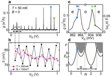
Figure 3: Even-odd Coulomb peak spacings a, Measured zero-bias conductance, $g$, versus gate voltage, $V_{\mathrm{G}}$, at temperature $T\sim 50~{}\mathrm{mK}$, and magnetic field $B=0$. b, Peak spacing, $S$, versus gate voltage. Black points show spacings from a calculated using the peak centroid (first moment), red points $T=350~{}\mathrm{mK}$ and $B=0$, purple points $B=150~{}\mathrm{mT}$ and $T\sim 50~{}\mathrm{mK}$. c, Right-most peaks in a. Peak maxima ($\triangle$) and centroids ($\blacksquare$) are marked. d, Free energy, $F$, at $T=0$ versus gate-induced charge, $N$, for different HQD occupations, where $N=CV_{\mathrm{G}}/e$ up to an offset and $C$ is the gate capacitance. Parabola intersection points are indicated by circles, corresponding to Coulomb peaks. BCS continuum (shaded), shown for odd occupancy. Odd Coulomb diamonds carry an energy offset $E_{0}$ for quasiparticle occupation of the sub gap state, resulting in a difference in spacing for even and odd diamonds.

Measured and model conductances are compared in Figs. 2a,b. The coupling of the bound state to each lead, noting the near-symmetry of the diamonds, was estimated to be $\Gamma_{0}=0.5~{}\mathrm{GHz}$, based on zero-bias conductance (Fig. 2d). The energy of the discrete state, $E_{0}=58~{}\mathrm{\mu eV}$ at zero magnetic field, was measured using finite bias spectroscopy (Fig. 2e). The normal-state conductance from each lead to the continuum, $g_{\mathrm{Al}}=0.15~{}e^{2}/h$, was estimated by comparing Coulomb blockaded transport features in the high bias regime ($V_{\mathrm{SD}}=0.4~{}\mathrm{mV}$). The superconducting gap, $\Delta=180~{}\mathrm{\mu eV}$, was found from the onset of NDC, which is expected to occur at $eV_{\mathrm{SD}}=\Delta-E_{0}$ (Fig. 2f). While the rate model shows good agreement with experimental data, some features are not captured, including broadening at high bias, with greater broadening correlated with weaker NDC, and peak-to-peak fluctuations in the slope of the NDC feature. These features may be related to heating or cotunneling, not accounted for by the model.

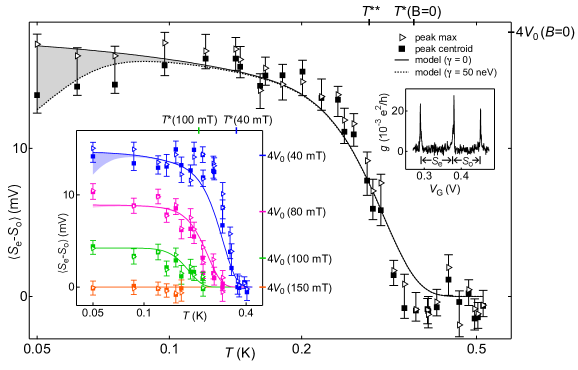
Figure 4: Temperature and magnetic field dependence of the even-odd peak spacings. Average even-odd spacing difference, $\left<S_{\mathrm{e}}-S_{\mathrm{o}}\right>$, versus temperature, $T$. Spacing between peak maxima (triangle) and centroids (square) are shown. Spacing expected from lower Zeeman-split bound state, $4V_{0}(B)=4E_{0}(B)/(\alpha e)$, indicated on right axis. Quasiparticle activation temperature, $T^{*}$, and crossover temperature, $T^{**}$, indicated on top axis. Solid curve is Eq. (1) with a HQD density of states measured from Fig. 2 ($\Delta=180~{}\mathrm{\mu eV}$, $E_{0}=58~{}\mathrm{\mu eV}$, $\alpha=0.013$), and the fitted aluminum volume, $V=7.4\times 10^{4}~{}\mathrm{nm^{3}}$. Dotted curve includes a discrete state broadening, $\gamma=50~{}\mathrm{neV}$, fit to the centroid data. Left inset: Same as main, but at $B=40,80,100,150~{}\mathrm{mT}$, from top to bottom. Curves are fit to two shared parameters: g-factor, $g=6$, and superconducting critical field, $B_{\mathrm{c}}=120~{}\mathrm{mT}$, with other parameters fixed from main figure. Right inset: Representative Coulomb peaks showing even ($S_{\mathrm{e}}$) and odd ($S_{\mathrm{o}}$) spacings.

The observation of negative differential conductance places a bound on the relaxation rate of a single quasiparticle in the HQD from the continuum (in the Al) to the bound state (in the InAs nanowire). Negative differential conductance arises when an electron tunnels into the weakly coupled BCS continuum, blockading transport until it exits via the lead. The blocking condition is shown for a hole-like excitation in Fig. 2f. Unblocking occurs when the quasiparticle relaxes into the bound state, followed by a fast escape to the leads. NDC thus indicates a long quasiparticle relaxation time, $\tau_{\mathrm{qp}}$, from the continuum to the bound state. Using independently determined parameters, the observed NDC is only compatible with the model when $\tau_{\text{qp}}>0.1~{}\mathrm{\mu s}$ (see Supplement). This bound on $\tau_{\text{qp}}$ is used below to similarly constrain the characteristic poisoning time for the bound state.

Turning our attention to the even-odd structure of zero-bias Coulomb peaks (Figs. 3a,b), we observed consistent large-small peak spacings (Fig. 3), associating the larger spacings with even occupation, as expected theoretically Averin:1992hy ; Matveev:1994fq and already evident in Fig. 1. Occasional even-odd parity reversals on the timescale of hours were observed in some devices, similar to what is seen in metallic devices Maisi:2013cr . Peak spacing alternation disappears at higher magnetic fields, $B$, consistent with the superconducting-to-normal transition, and also disappears at elevated temperature, $T>0.4~{}\mathrm{K}$, significantly below the superconducting critical temperature, $T_{c}\sim 1~{}\mathrm{K}$. The temperature dependence is consistent with similar behavior seen in metallic structures Tuominen:1992ip ; Lafarge:1993vn , and can be understood as the result of thermal activation of quasiparticles within the HQD with fixed total charge.

As seen in Fig. 3c, individual Coulomb peaks are asymmetric in shape, with their centroids (first moments) on the even sides of the peak maxima. Note that the asymmetry leads to higher near-peak conductance in even valleys, the opposite of the Kondo effect. The asymmetric shape is most pronounced at low temperature, $T<0.15~{}\mathrm{K}$, and decreases with increasing magnetic field. The degree of asymmetry is not predicted by the rate model, even taking into account the known small asymmetry due to spin degeneracy Aleiner:2002in . In the analysis below, we consider peak positions defined both by peak maxima and centroids.

A model of even-odd Coulomb peak spacing that includes thermal quasiparticle excitations follows earlier treatments Tuominen:1992ip ; Lafarge:1993vn ; Matveev:1994fq , including a discrete subgap state as well as the BCS continuum Lafarge:1993vn (Fig. 3d). Even-odd peak spacing difference, $S_{\mathrm{e}}-S_{\mathrm{o}}$, depends on the difference of free energies,

$$S_{\mathrm{e}}-S_{\mathrm{o}}=\frac{4}{\alpha e}\left(F_{\mathrm{o}}-F_{\mathrm{e}}\right),$$ (1)

where $\alpha$ is the (dimensionless) gate lever arm. The free energy difference, written in terms of the ratio of partition functions,

$$F_{\mathrm{o}}-F_{\mathrm{e}}=-k_{\mathrm{B}}T\ln\left(\frac{Z_{\mathrm{o}}}{Z_{\mathrm{e}}}\right),$$ (2)

depends on $D(E)$, the density of states of the HQD,

$$\frac{Z_{\mathrm{o}}}{Z_{\mathrm{e}}}=\int_{0}^{\infty}\!\mathrm{d}E\ D(E)\ln\coth[E/(2k_{\mathrm{B}}T)],$$ (3)

where $D(E)$ consists of one subgap state and the continuum. For $\Delta\gg k_{\mathrm{B}}T$, this can be written

$$F_{\mathrm{o}}-F_{\mathrm{e}}\approx-k_{\mathrm{B}}T\ln(N_{\mathrm{eff}}e^{-\Delta/k_{\mathrm{B}}T}+2e^{-E_{0}/k_{\mathrm{B}}T}),$$ (4)

where $N_{\mathrm{eff}}=\rho_{\mathrm{Al}}V\sqrt{2\pi k_{\mathrm{B}}T\Delta}$ is the effective number of continuum states for Al volume, $V$, and normal density of states $\rho_{\mathrm{Al}}$ Tuominen:1992ip ; Lafarge:1993vn (see Supplement).

Within this model, one can identify a characteristic temperature, $T^{*}\sim\Delta/[k_{\mathrm{B}}\ln(N_{\mathrm{eff}})]$, less than the gap, above which even-odd peak spacing alternation is expected to disappear. Note in this expression $N_{\mathrm{eff}}$ itself depends on $T$, and also that $T^{*}$ does not depend on the bound state energy, $E_{0}$. A second (lower) characteristic temperature, $T^{**}\sim(\Delta-E_{0})/[k_{\mathrm{B}}\ln(N_{\mathrm{eff}}/2)]$, which does depend on $E_{0}$, is where the even-odd alternation is affected by the bound state, leading to saturation at low temperature Tuominen:1992ip ; Lafarge:1993vn . For a spin-resolved zero-energy ($E_{0}=0$) bound state—the case for unsplit Majorana zero modes—these characteristic temperatures coincide and even-odd structure vanishes, as pointed out in Ref. Fu:2010ho . In the opposite case, where the bound state reaches the continuum ($E_{0}=\Delta$), the saturation temperature vanishes, $T^{**}=0$, and the metallic result with no bound state is recovered Tuominen:1992ip ; Lafarge:1993vn .

Experimentally, the average even-odd peak spacing difference, $\langle S_{\mathrm{e}}-S_{\mathrm{o}}\rangle$, was determined by averaging over a set of 24 consecutive Coulomb peak spacings, including those shown in Fig. 3, at each temperature. Figure 4 shows even-odd peak spacing difference appearing abruptly at $T_{\mathrm{onset}}\sim 0.4$ K, and saturating at $T_{\mathrm{sat}}\sim 0.2$ K, with a saturation amplitude near the value expected from the measured bound state energy, $4V_{0}=4E_{0}/(\alpha e)$. Figure 4 shows good agreement between experiment and the model, Eq. (1), using a density of states determined independently from data in Fig. 2, with $V=7.4\times 10^{4}~{}\mathrm{nm^{3}}$ as a fit parameter, consistent with the micrograph (Fig. 1a), and $\rho_{\mathrm{Al}}=23~{}\mathrm{eV^{-1}nm^{-3}}$ Maisi:2013cr .

The asymmetric peak shape complicates measurement of even-odd spacings, as one can either use the centroids or maxima to measure spacings, the two methods giving different results. Larger peak tails on the even valley side cause the centroids to be more regularly spaced than the maxima. This is evident in Fig. 4, where the centroid method shows a decreasing peak spacing difference at low temperature, while with the maximum method the spacing remains flat. The thermal model of $S_{\mathrm{e}}-S_{\mathrm{o}}$ can also show a decrease at low temperature if broadening of the bound state is included (See Methods). We do not understand at present if the low temperature decrease in the centroid data is related to the decrease seen in the model when broadening is included. It is worth noting, however, that the fit to the centroid data gives a broadening $\gamma=50~{}\mathrm{neV}$, reasonably close to the value estimated from the lead couplings, $(h\Gamma_{0})^{2}/\Delta=20~{}\mathrm{neV}$.

Applied magnetic field (direction shown in Fig. 1b) reduces the characteristic temperatures $T_{\mathrm{onset}}$, $T_{\mathrm{sat}}$, and saturation amplitudes. Field dependence is modeled by including Zeeman splitting of the bound state and orbital reduction of the gap and bound state energy, taking the $g$-factor and critical magnetic field as two fit parameters applied to all data sets. The fit value $g=6$ lies within the typical range for InAs nanowires Bjork:2005hx ; Csonka:2008gz , supporting our interpretation of the bound state residing in the InAs. The fit value of critical field, $B_{\mathrm{c}}=120~{}\mathrm{mT}$, is typical for this geometry.

Good agreement between the peak spacing data and the thermodynamic model (Fig. 4) suggests that the number of thermally activated quasiparticles obeys equilibrium statistics, $N_{\mathrm{eq}}(T)=N_{\mathrm{eff}}^{2}e^{-2\Delta/k_{\mathrm{B}}T}$ (see Supplement for derivation). Saturation caused by the bound state means that even-odd amplitude loses sensitivity as a quasiparticle detector below $T_{\mathrm{sat}}$. We therefore take $N_{\mathrm{eq}}(T_{\mathrm{sat}})\sim 10^{-5}$ (for $T_{\mathrm{sat}}\sim 0.2$ K) as an upper bound for the number of quasiparticles at temperatures below $T_{\mathrm{sat}}$. The corresponding upper bound of the quasiparticle fraction, $x_{\mathrm{qp}}=N_{\mathrm{eq}}(T_{\mathrm{sat}})/(\rho_{\mathrm{Al}}V\Delta)\sim 10^{-8}$, is comparable to values in the recent literature, $10^{-5}-10^{-8}$, for metallic superconducting junctions and qubits Martinis:2009bd ; DeVisser:2011bm ; Saira:2012ca ; Riste:2013il ; Pop:2014gg .

We now discuss the implications of our measurements for determining the poisoning time, $\tau_{\mathrm{p}}$, of the bound state. For the present geometry, the dominant source of poisoning of the bound state is not tunneling of electrons from the leads, which is negligible in the strongly blockaded regime, but is rather the continuum in the strongly-coupled Al, within the isolated structure itself. Theoretical estimates Rainis:2012uw suggest an inverse relationship between $\tau_{p}$ and the number of available quasiparticles, with a proportionality that depends on system details. Taking the bound on single quasiparticle relaxation time from the continuum into the bound state, $\tau_{\text{qp}}>0.1~{}\mathrm{\mu s}$, from above, as the poisoning time when a single quasiparticle is present, we estimate $\tau_{p}$ by scaling for the actual number of quasiparticles in equilibrium, $N_{\mathrm{eq}}$, giving a poisoning time $\tau_{\mathrm{p}}=\tau_{\mathrm{qp}}/N_{\mathrm{eq}}\gtrsim 10~{}\mathrm{ms}$.

We expect $\tau_{p}$ to depend weakly on the bound state energy for low-energy bound states Zgirski:2011wp ; Olivares:2014ig ; Zazunov:2014kn , including for Majorana zero modes at $E_{0}=0$. Device geometry may somewhat alter the number of quasiparticles available to relax into the bound state, i.e. by changing $N_{\mathrm{eff}}$, but any increase can be compensated by exponentially small decreases in the quasiparticle temperature. The long poisoning time obtained here suggests that a large number of braiding operations in Majorana systems should be readily achievable within the relevant time scale.

Methods

Sample preparation: InAs nanowires were grown in the [001] direction with wurzite crystal structure with Al epitaxially matched to [111] on two of the six $\{1\bar{1}00\}$ sidefacets. They were then deposited randomly onto a doped silicon substrate with 100 nm of thermal oxide. Electron-beam lithographically patterned wet etch of the epitaxial Al shell (Transene Al Etchant D, 55 C, 10 s) resulted in a submicron Al segment (310 nm, Fig. 1a). Ti/Au (5/100 nm) ohmic contacts were deposited on the ends following in situ Ar milling (1 mTorr, 300 V, $75~{}\mathrm{s}$), with side gates deposited in the same step. For the present device, the end of the upper left gate broke off during processing. However, the device could be tuned well without it.

Master equations: The master equations (used for Fig. 1b) consider states with fixed total parity, composed of the combined parity of quasiparticles in the thermalized continuum and the 0, 1, or 2 quasiparticles in the bound state (see Supplement).

Free energy model: Even and odd partition functions in Eq. 2, $F_{\mathrm{o}}-F_{\mathrm{e}}=-k_{\mathrm{B}}T\ln(Z_{\mathrm{o}}/Z_{\mathrm{e}})$, can be written as sums of Boltzmann factors over respectively odd and even occupancies of the isolated island. For even-occupancy,

$$Z_{\mathrm{e}}=1+\sum_{i\neq j}e^{-E_{i}/k_{\mathrm{B}}T}e^{-E_{j}/k_{\mathrm{B}}T}+...,$$ (5)

where the first term stands for zero quasiparticles, the second for two (at energies $E_{i}$ and $E_{j}$), and additional terms for four, six, etc. $Z_{\mathrm{o}}$ similarly runs over odd occupied states. Rewriting these sums as integrals over positive energies yields

$$F_{\mathrm{o}}-F_{\mathrm{e}}=-k_{\mathrm{B}}T\ln\tanh\int_{0}^{\infty}\!\mathrm{d}E\ D(E)\ln\coth(E/2k_{\mathrm{B}}T),$$ (6)

where $D(E)$ is the density of states of the HQD,

$$D(E)=\rho_{\mathrm{BCS}}(E)+\frac{1}{2}\rho_{\mathrm{0}}^{+}(E)+\frac{1}{2}\rho_{\mathrm{0}}^{-}(E).$$ (7)

We take $\rho_{\mathrm{BCS}}(E)$ to be a standard BCS density of states,

$$\rho_{\mathrm{BCS}}(E)=\frac{\rho_{\mathrm{Al}}VE}{\sqrt{E^{2}-\Delta(B)^{2}}}\theta(E-\Delta)$$ (8)

($\theta$ is the step function), and $\rho_{0}$ to be a pair of Lorentzian-broadened spinful levels symmetric about zero,

$$\rho_{0}^{\pm}(E)=\frac{\gamma/2\pi}{(E-E^{\pm}_{0})^{2}+(\gamma/2)^{2}}+\frac{\gamma/2\pi}{(E+E^{\pm}_{0})^{2}+(\gamma/2)^{2}}.$$ (9)

Zeeman splitting of the bound state and pair-breaking by the external magnetic field are modeled with the equations

$$E_{0}^{\pm}(B) = \frac{\Delta(B)}{\Delta}E_{0}\pm\frac{1}{2}g\mu_{B}B,$$ (10)

$$\Delta(B) = \Delta\sqrt{1-\left(\frac{B}{B_{c}}\right)^{2}},$$ (11)

where $E_{\mathrm{0}}$ is the zero-field state energy and $\Delta$ is the zero field superconducting gap. In the event that a bound state goes above the continuum, $E_{s}^{+}>\Delta(B)$, we no longer include the state in the free energy. Equation (6) was integrated numerically to obtain theory curves in Fig. (4).

Equations (10) and (11) are reasonable provided the lower spin-split state remains at positive energy, $E_{0}^{-}>0$. For sufficiently large $B_{c}$, the bound state will reach zero energy, resulting in topological superconductivity and Majorana modes, the subject of future work.

We thank Leonid Glazman, Bert Halperin, Roman Lutchyn and Jukka Pekola for valuable discussions, and Giulio Ungaretti, Shivendra Upadhyay and Claus Sørensen for contributions to growth and fabrication. Research support by Microsoft Project Q, the Danish National Research Foundation, the Lundbeck Foundation, the Carlsberg Foundation, and the European Commission. APH acknowledges support from the US Department of Energy, CMM acknowledges support from the Villum Foundation.

Section I Supplementary Information:

Section II Quasiparticle parity dynamics in a superconductor-semiconductor hybrid quantum dot

1. Effective gate voltage definition

2. Bound on the single quasiparticle relaxation time

3. Detailed interpretation of Coulomb diamonds

4. Derivation of transport and thermal model

5. Comparison of free energy approximations

6. Effect of the bound state on the free energy

II.1 1. Effective gate voltage definition

We define an effective gate voltage in software to tune the HQD. The physical gate voltages, $V_{\mathrm{R}}$ and $V_{\mathrm{L}}$, are related to the effective gate voltage, $V_{\mathrm{G}}$, by

$$V_{\mathrm{R}} =V_{R,0}+\kappa~{}V_{\mathrm{G}},$$

$$V_{\mathrm{L}} =V_{L,0}+\sqrt{1-\kappa^{2}}~{}V_{\mathrm{G}},$$

with $\kappa=0.9997$ and offset voltages $V_{R,0}=-2.41~{}\mathrm{V}$, $V_{L,0}=-3.96~{}\mathrm{V}$.

These transformation rules ensure that $V_{G}^{2}=(V_{R}-V_{R,0})^{2}+(V_{L}-V_{L,0})^{2}$, so that $V_{G}$ can be interpreted as the distance from $(V_{R,0},V_{L,0})$ in the $V_{R}-V_{L}$ plane.

All measurements are performed at backgate voltage $V_{\mathrm{BG}}=2.39~{}\mathrm{V}$.

II.2 2. Bound on the single quasiparticle relaxation time

The effect of quasiparticle relaxation is shown in Figs. S1a-e. Quasiparticle relaxation results in a disappearance of the negative differential conductance, in combination with the appearance of an extra conductance threshold. We quantify this observation by introducing the relative conductance ratio

$$R=\frac{g^{\prime}+g_{\mathrm{NDC}}}{g^{\prime}-g_{\mathrm{NDC}}}$$ (S1)

where $g_{\mathrm{NDC}}$ is the minimum of the negative differential conductance, and $g^{\prime}$ is the maximum of the extra conductance threshold that appears when $\tau_{\mathrm{qp}}\rightarrow 0$ (see Fig. S1i). The $R$-value is a metric for the relative strength of the negative differential conductance.

Figs. S1f-j show example conductance traces at constant bias and their associated $R$-values. The traces show that $R\approx-1$ corresponds to slow quasiparticle relaxation, and $R\approx 1$ corresponds to fast quasiparticle relaxation.

Fig. S2 shows the $R$-value calculated as a function of single quasiparticle relaxation time, $\tau_{\mathrm{qp}}$. Also shown is a measured $R$-value averaged over all negative differential conductance features in Fig. 1 of the main text. The measured $R$-value is consistent with $\tau_{\mathrm{qp}}>0.1~{}\mathrm{\mu s}$, giving the experimental bound on the single quasiparticle relaxation time.

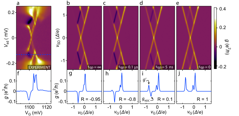
Fig. S1: Effect of quasiparticle relaxation. a Measured conductance $g$ versus source-drain bias $V_{\mathrm{SD}}$ and gate $V_{\mathrm{G}}$. b, Transport model of a, with $\tau_{\mathrm{qp}}=\infty$. $v_{\text{G}}\equiv\alpha V_{\mathrm{G}}$ up to an offset, where $\alpha$ is the gate lever arm. Axis units are $\Delta/e=180~{}\mathrm{\mu V}$. c-e, Model with $\tau_{\mathrm{qp}}=0.1~{}\mathrm{\mu s}$, $\tau_{\mathrm{qp}}=5~{}\mathrm{ns}$, and $\tau_{\mathrm{qp}}=0$ respectively. f-j, Conductance versus gate at constant bias indicated in a. Relative conductance ratio, $R=(g^{\prime}+g_{\mathrm{NDC}})/(g^{\prime}-g_{\mathrm{NDC}})$, for theory curves is labeled (see text).

Fig. S2: Single quasiparticle relaxation bound. Relative conductance ratio, $R=(g^{\prime}+g_{\mathrm{NDC}})/(g^{\prime}-g_{\mathrm{NDC}})$, versus single quasiparticle relaxation time $\tau_{\mathrm{qp}}$. Dashed curve is theory derived as shown in Fig. S1. Data is the average over all charge transitions in Fig. 1, with vertical error the standard deviation of the mean, and horizontal error propagated from vertical.

II.3 3. Detailed interpretation of Coulomb diamonds

Each conductance threshold in the Coulomb diamond plots can be interpreted with the help of the transport model, as shown in Fig. S3. For example, the highest bias at which NDC is observed occurs at the intersection of black and green lines, when $v_{\mathrm{SD}}=(\Delta+E_{0})/e$.

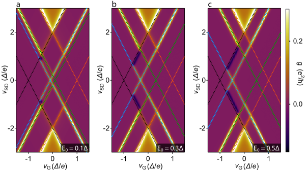
Fig. S3: Interpreting conductance thresholds. a, Calculated conductance $g$ versus $v_{\mathrm{SD}}$ and $v_{\mathrm{G}}$. $E_{0}=0.1\Delta$, all other model parameters same as main text. Dotted lines are $v_{\mathrm{SD}}/2=\pm(v_{\mathrm{G}}+\Delta/e)$ [black], $v_{\mathrm{SD}}/2=\pm(v_{\mathrm{G}}+E_{0}/e)$ [blue], $v_{\mathrm{SD}}/2=\pm(v_{\mathrm{G}}-E_{0}/e)$ [green], $v_{\mathrm{SD}}/2=\pm(v_{\mathrm{G}}-\Delta/e)$ [red]. b, $E_{0}=0.32\Delta$, all model parameters same as main text. c, $E_{0}=0.5\Delta$, all other model parameters same as main text. Color scale shared across all plots.

II.4 4. Derivation of transport and thermal model

This section gives a detailed derivation of the transport and thermal model used in the main text.

To describe the electron transport through a metallic superconducting quantum dot we consider the following model:

$$H=H_{\mathrm{LR}}+H_{\mathrm{D}}+H_{\mathrm{T}},$$ (S2)

where the Hamiltonian

$$H_{\mathrm{LR}}=\sum_{\alpha\nu s}\left(\varepsilon_{\alpha\nu s}-\mu_{\alpha}\right)c^{{\dagger}}_{\alpha\nu s}c^{\phantom{{\dagger}}}_{\alpha\nu s}$$ (S3)

describes the normal metallic leads with $c^{{\dagger}}_{\alpha\nu s}$ being an electron creation operator in the lead $\alpha\in\{\mathrm{L},\mathrm{R}\}$, with an orbital quantum number $\nu$ and spin $s\in\{\uparrow,\downarrow\}$. The leads have chemical potentials given by $\mu_{\alpha}=\pm V/2$, where $V$ denotes symmetrically applied bias. For the semiconductor-superconductor hybrid quantum dot, we use a simplified model consisting of a Bardeen-Cooper-Schrieffer (BCS)Bardeen et al. (1957) continuum and an Andreev bound state for fixed number of particles Tinkham (1972):

$$H_{\mathrm{D}}=\sum_{s,p=e,h}\Big{[}E_{0}\gamma^{{\dagger}}_{0s,p}\gamma^{\phantom{{\dagger}}}_{0s,p}+\sum_{n}E_{n}\gamma^{{\dagger}}_{ns,p}\gamma^{\phantom{{\dagger}}}_{ns,p}\Big{]}+E_{N}^{c},$$ (S4)

$$\quad E_{N}^{c}=U(N-N_{g})^{2},\quad N=\Big{[}\sum_{s}d^{{\dagger}}_{0s}d^{\phantom{{\dagger}}}_{0s}+\sum_{n}d^{{\dagger}}_{ns}d^{\phantom{{\dagger}}}_{ns}\Big{]},$$ (S5)

where $d^{{\dagger}}_{ns}$ creates an electron in the continuum with quantum number $n$ (e.g. momentum of electrons on the dot), and $d^{{\dagger}}_{0s}$ denotes electron creation in a localized level, which gives rise to a subgap state in the BCS spectrum. The charging effects on the quantum dot are described by constant interaction model given by the term $E_{N}^{c}$, where the charging energy is given by $E_{C}=2U$ and the number of electrons on the dot is controlled by a gate voltage $V_{g}$, which is parameterized by dimensionless number $N_{g}=V_{g}/E_{C}$. The operator $N$ gives the total number of electrons on the dot. With superconducting pairing, the dot Hamiltonian is diagonal in the basis of the quasiparticle operators $\gamma^{{\dagger}}$, which are given by Josephson (1962); Bardeen (1962); Tinkham (2004)

$$d^{\phantom{{\dagger}}}_{ns}=u_{n}\gamma^{\phantom{{\dagger}}}_{ns,e}+sv_{n}\gamma^{{\dagger}}_{-n\bar{s},h},$$ (S6a)

$$\gamma^{\phantom{{\dagger}}}_{ns,e}=u_{n}d^{\phantom{{\dagger}}}_{ns}-sv_{n}d^{{\dagger}}_{-n\bar{s}}S,$$ (S6b)

$$\gamma^{\phantom{{\dagger}}}_{ns,h}=u_{n}S^{{\dagger}}d^{\phantom{{\dagger}}}_{ns}-sv_{n}d^{{\dagger}}_{-n\bar{s}},$$ (S6c)

$$\gamma^{{\dagger}}_{ns,e}=S^{{\dagger}}\gamma^{{\dagger}}_{ns,h},\quad\gamma^{\phantom{{\dagger}}}_{ns,h}=S^{{\dagger}}\gamma^{\phantom{{\dagger}}}_{ns,e},$$ (S6d)

with $S^{{\dagger}}$ denoting the Cooper pair creation operator and $\gamma^{{\dagger}}_{ns,e/h}$ denoting the quasiparticle creation operator, which adds an electron/hole to the system. Here a state with quantum numbers $-ns$ is the time-reversed partner of a state with quantum numbers $ns$. The quasiparticle excitation energy $E_{n}$ and the BCS coherence factors $u_{n},\ v_{n}$ are given in terms of superconducting gap $\Delta$ and electron dispersion on the dot $\varepsilon_{n}$ as

$$E_{n}=\sqrt{\varepsilon_{n}^{2}+\Delta^{2}},\quad u_{n}=\sqrt{\frac{1}{2}\left(1+\frac{\varepsilon_{n}}{E_{n}}\right)},\quad v_{n}=\sqrt{\frac{1}{2}\left(1-\frac{\varepsilon_{n}}{E_{n}}\right)}.$$ (S7)

Similarly, the subgap state operator is expressed as

$$d^{\phantom{{\dagger}}}_{0s}=u_{0}\gamma^{\phantom{{\dagger}}}_{0s,e}+sv_{0}\gamma^{{\dagger}}_{0\bar{s},h},$$ (S8)

with $u_{0}$, $v_{0}$ being model dependent coherence factors, which we set to $u_{0}=v_{0}=1/\sqrt{2}$ for simplicity. Lastly, the electrons in the leads and in the dot are coupled by the tunneling

$$H_{\mathrm{T}} =\sum_{\begin{subarray}{c}\alpha\nu s\end{subarray}}\Big{[}t_{\mathrm{S},\alpha}c^{{\dagger}}_{\alpha\nu s}d^{\phantom{{\dagger}}}_{0s}+t_{\mathrm{S},\alpha}^{*}d^{{\dagger}}_{0s}c^{\phantom{{\dagger}}}_{\alpha\nu s}+\sum_{n}\left(t_{\mathrm{C},\alpha}c^{{\dagger}}_{\alpha\nu s}d^{\phantom{{\dagger}}}_{ns}+t_{\mathrm{C},\alpha}^{*}d^{{\dagger}}_{ns}c^{\phantom{{\dagger}}}_{\alpha\nu s}\right)\Big{]}$$ (S9)

$$\begin{aligned} =\sum_{\begin{subarray}{c}\alpha\nu s\end{subarray}}\Big{[}&t_{\mathrm{S},\alpha}c^{{\dagger}}_{\alpha\nu s}(u_{0}\gamma^{\phantom{{\dagger}}}_{0s,e}+sv_{0}\gamma^{{\dagger}}_{0\bar{s},h})+t_{\mathrm{S},\alpha}^{*}(u_{0}^{*}\gamma^{{\dagger}}_{0s,e}+sv_{0}^{*}\gamma^{\phantom{{\dagger}}}_{0\bar{s},h})c^{\phantom{{\dagger}}}_{\alpha\nu s}\\ +\sum_{n}\big{\{}&t_{\mathrm{C},\alpha}c^{{\dagger}}_{\alpha\nu s}(u_{n}\gamma^{\phantom{{\dagger}}}_{ns,e}+sv_{n}\gamma^{{\dagger}}_{-n\bar{s},h})+t_{\mathrm{C},\alpha}^{*}(u_{n}^{*}\gamma^{{\dagger}}_{ns,e}+sv_{n}^{*}\gamma^{\phantom{{\dagger}}}_{-n\bar{s},h})c^{\phantom{{\dagger}}}_{\alpha\nu s}\big{\}}\Big{]},\end{aligned}$$

where $t_{\mathrm{C},\alpha}$ gives the tunneling amplitude to the continuum and $t_{\mathrm{S},\alpha}$ gives the tunneling amplitude to the subgap state.

II.4.1 Thermodynamics of the even/odd effect

We now present the free energy difference between the superconducting metallic island having even or odd number of electrons. The parity of the number of quasiparticles has to be equal to the parity of the number of electrons $N$ on the island. The free energy difference $\delta{F}$ between the odd and even occupation is expressed as Tuominen et al. (1992); Lafarge et al. (1993)

$$\delta{F}=F_{\mathrm{o}}-F_{\mathrm{e}}=-\frac{1}{\beta}\ln\left(\frac{Z_{\mathrm{o}}}{Z_{\mathrm{e}}}\right),$$ (S10)

in terms of the partition functions for different parities

$$2Z_{\mathrm{o}/\mathrm{e}}=\prod_{n,s}(1+e^{-\beta E_{n}})\mp\prod_{n,s}(1-e^{-\beta E_{n}}).$$ (S11)

where $\beta=1/k_{\mathrm{B}}T$ denotes the inverse temperature of the island. For a sufficiently large island the single particle spectrum can be described by the spectrum of a grounded superconductor where the single particle spectrum $E_{n}$ is given by Eq. (S7).

Without a subgap state the free energy difference Eq. (S10) is expressed as

$$\delta{F}_{\mathrm{BCS}}=-k_{\mathrm{B}}T\ln\tanh\left[\frac{1}{2}\sum_{n,s}\ln\coth\left(\frac{\beta E_{n}}{2}\right)\right]=-\frac{1}{\beta}\ln\tanh\int_{\Delta}^{+\infty}\mathrm{d}E\,\rho_{\mathrm{BCS}}(E)\ln\coth\left(\frac{\beta E}{2}\right),$$ (S12)

where $\rho_{\mathrm{BCS}}(E)$ is the BCS density of states for quasiparticles on the island given by

$$\rho_{\mathrm{BCS}}(E)=\frac{\rho_{\mathrm{D}}E}{\sqrt{E^{2}-\Delta^{2}}},$$ (S13)

with $\rho_{\mathrm{D}}=\rho_{\mathrm{Al}}V$ denoting the normal state density of states, including spin, and $\rho_{\mathrm{Al}}$ is aluminum density of states per volume, and $V$ is the volume of the island. For small temperatures $\beta\Delta\gg 1$, the free energy difference (S12) can be approximated as

$$\delta{F}_{\mathrm{BCS}}\approx-k_{\mathrm{B}}T\ln\tanh\left[2\int_{\Delta}^{+\infty}\mathrm{d}E\,\rho_{\mathrm{BCS}}(E)e^{-\beta E}\right]=-k_{\mathrm{B}}T\ln\tanh\left[N_{\mathrm{eff}}e^{-\beta\Delta}\right]\approx\Delta-k_{\mathrm{B}}T\ln(N_{\mathrm{eff}}),$$ (S14)

where an effective number of quasiparticle states $N_{\mathrm{eff}}$ is given by

$$N_{\mathrm{eff}}=2\int_{\Delta}^{+\infty}\mathrm{d}E\,\rho_{\mathrm{BCS}}(E)e^{-\beta(E-\Delta)}=2\rho_{\mathrm{D}}\Delta e^{\beta\Delta}K_{1}(\beta\Delta)\approx\rho_{\mathrm{D}}\sqrt{2\pi k_{\mathrm{B}}T\Delta}$$ (S15)

and $K_{\nu}(x)$ denotes the modified Bessel function of the second kind.

With a subgap state the free energy difference Eq. (S10) acquires an additional term and one gets

$$\delta{F}_{\mathrm{ABS}}=-k_{\mathrm{B}}T\ln\tanh\left[\int_{\Delta}^{+\infty}\mathrm{d}E\,\rho_{\mathrm{BCS}}(E)\ln\coth\left(\frac{\beta E}{2}\right)+\ln\coth(\beta E_{0}/2)\right].$$ (S16)

See also Eq. (S42) where the approximate expression for the first term in used.

In the main text we discuss how the low-temperature data deviates from the above Andreev-bound-state model in terms of a life-time broadening of the subgap state. This is done by including a phenomenological broadening with width $\gamma$ into the subgap density of states, which then gives the free energy difference

$$\delta{F}_{\mathrm{ABS-LB}}=-k_{\mathrm{B}}T\ln\tanh\Bigg{[}\int_{\Delta}^{+\infty}\mathrm{d}E\,\rho_{\mathrm{BCS}}(E)\ln\coth\left(\frac{\beta E}{2}\right)+\frac{1}{2}\sum_{\begin{subarray}{c}\tau=\pm 1\\ s=\uparrow,\downarrow\end{subarray}}\int_{0}^{+\infty}\frac{\mathrm{d}\omega\,}{2\pi}\frac{\gamma\ln\coth\left(\frac{\beta\omega}{2}\right)}{(\omega-\tau E_{0})^{2}+(\gamma/2)^{2}}\Bigg{]}.$$ (S17)

In the kinetic equation calculation presented below, the equilibrium distributions of quasiparticle in the continuum with an even or odd number of quasiparticles are needed. Since we will assume that the particles occupying the continuum are effectively equilibrated, we find the distribution functions by modifying the usual Fermi-Dirac distribution function as

$$f_{P}(E)=\frac{1}{e^{\beta E}(Z_{P}/Z_{\bar{P}})+1}\quad\rightarrow\quad\left\{\begin{aligned} &f_{\mathrm{e}}(E)=\frac{1}{e^{\beta(E+\delta{F}_{\mathrm{BCS}})}+1},\\ &f_{\mathrm{o}}(E)=\frac{1}{e^{\beta(E-\delta{F}_{\mathrm{BCS}})}+1},\end{aligned}\right.$$ (S18)

where $P\in\{\mathrm{e},\mathrm{o}\}$, and $\bar{P}$ represents the opposite of $P$.

II.4.2 Number of quasiparticles

Using the above results, we derive a simple expression for the number of quasiparticles in the absence of a bound state. At low temperature, when $\delta{F}_{\mathrm{BCS}}=\Delta-k_{\mathrm{B}}T\ln(N_{\mathrm{eff}})$, the distribution functions take the form

$$f_{\mathrm{e}} = N_{\mathrm{eff}}e^{-\beta(E+\Delta)},$$ (S19)

$$f_{\mathrm{o}} = \frac{1}{N_{\mathrm{eff}}}e^{-\beta(E-\Delta)},$$ (S20)

where $N_{\mathrm{eff}}$ is given by Eq. (S15).

The number of quasiparticles in each parity state can then be calculated using

$$N_{P}=2\int_{\Delta}^{+\infty}\mathrm{d}E\,\rho_{\mathrm{BCS}}(E)f_{P}(E).$$ (S21)

Substituting the above expression for $f_{\mathrm{o}}$ gives $N_{\mathrm{o}}=1$, as expected. Substituting $f_{\mathrm{e}}$ gives the quasiparticle number

$$N_{\mathrm{e}} = 2\int_{\Delta}^{+\infty}\mathrm{d}E\,\rho_{\mathrm{BCS}}(E)N_{\mathrm{eff}}e^{-\beta(E+\Delta)}$$ (S22)

$$= N_{\mathrm{eff}}e^{-2\beta\Delta}\int_{\Delta}^{+\infty}\mathrm{d}E\,~{}2\rho_{\mathrm{BCS}}(E)e^{-\beta(E-\Delta)}$$

$$= \left(N_{\mathrm{eff}}e^{-\beta\Delta}\right)^{2}.$$

Because of the large charging energy $N_{\mathrm{e}}$ is the square of the bulk value $N_{\mathrm{eff}}e^{-\beta\Delta}$, indicating that quasiparticles must be created in pairs.

II.4.3 Incoherent transport

We now calculate the current through the quantum dot by a set of master equations, with transition rates calculated by Fermi’s golden rule, which is valid in the weak tunneling regime or the so-called sequential tunneling regime.

According to the Fermi’s golden rule the transition rate from the initial state $i$ to the final state $j$ caused by a perturbation $V$ is given by Bruus and Flensberg (2004):

$$\Gamma_{fi}=2\pi\lvert\langle f\rvert V\lvert i\rangle\rvert^{2}\delta(E_{f}-E_{i}).$$ (S23)

In our case we are interested in the transitions caused by the tunneling Hamiltonian (S9) between the states $\lvert\mathcal{D}\rangle\lvert\mathrm{LR}\rangle$ and $\lvert\mathcal{D^{\prime}}\rangle\lvert\mathrm{LR}^{\prime}\rangle$:

$$\Gamma_{\mathcal{D}^{\prime}\mathcal{D},\mathrm{LR}^{\prime}\mathrm{LR}}=2\pi\lvert\langle\mathrm{LR}^{\prime}\rvert\langle\mathcal{D}^{\prime}\rvert H_{\mathrm{T}}\lvert\mathcal{D}\rangle\lvert\mathrm{LR}\rangle\rvert^{2}\delta(E_{\mathcal{D}^{\prime}}-E_{\mathcal{D}}+E_{\mathrm{LR}^{\prime}}-E_{\mathrm{LR}}),$$ (S24)

where the many-body eigenstates of the lead Hamiltonian $H_{\mathrm{LR}}$ are denoted as $\lvert\mathrm{LR}\rangle$ and of the dot Hamiltonian $H_{\mathrm{D}}$ are denoted as $\lvert\mathcal{D}\rangle$. Also $E_{\mathcal{D}}$ gives the energy of the state $\lvert\mathcal{D}\rangle$ and $E_{\mathrm{LR}}$ gives the energy of the state $\lvert\mathrm{LR}\rangle$. So we see that we need the following matrix element

$$\lvert\langle\mathrm{LR}^{\prime}\rvert\langle\mathcal{D}^{\prime}\rvert H_{\mathrm{T}}\lvert\mathcal{D}\rangle\lvert\mathrm{LR}\rangle\rvert^{2}=\sum_{\begin{subarray}{c}\alpha\nu sn\end{subarray}}\lvert t_{\alpha}\rvert^{2}\Big{\{} \lvert u_{n}\rvert^{2}\lvert\langle\mathrm{LR}^{\prime}\rvert c^{{\dagger}}_{\alpha\nu s}\lvert\mathrm{LR}\rangle\rvert^{2}\lvert\langle\mathcal{D}^{\prime}\rvert\gamma^{\phantom{{\dagger}}}_{ns,e}\lvert\mathcal{D}\rangle\rvert^{2}$$ (S25)

$$+ \lvert v_{n}\rvert^{2}\lvert\langle\mathrm{LR}^{\prime}\rvert c^{{\dagger}}_{\alpha\nu s}\lvert\mathrm{LR}\rangle\rvert^{2}\lvert\langle\mathcal{D}^{\prime}\rvert\gamma^{{\dagger}}_{-n\bar{s},h}\lvert\mathcal{D}\rangle\rvert^{2}$$

$$+ \lvert u_{n}\rvert^{2}\lvert\langle\mathrm{LR}^{\prime}\rvert c^{\phantom{{\dagger}}}_{\alpha\nu s}\lvert\mathrm{LR}\rangle\rvert^{2}\lvert\langle\mathcal{D}^{\prime}\rvert\gamma^{{\dagger}}_{ns,e}\lvert\mathcal{D}\rangle\rvert^{2}$$

$$+ \lvert v_{n}\rvert^{2}\lvert\langle\mathrm{LR}^{\prime}\rvert c^{\phantom{{\dagger}}}_{\alpha\nu s}\lvert\mathrm{LR}\rangle\rvert^{2}\lvert\langle\mathcal{D}^{\prime}\rvert\gamma^{\phantom{{\dagger}}}_{-n\bar{s},h}\lvert\mathcal{D}\rangle\rvert^{2}\Big{\}}.$$

Note that we have not written out the terms with the subgap state, but they have an analogous structure.

In order to form the tunneling rates we need to specify what kind of states $\lvert\mathcal{D}\rangle$ on the metallic superconducting quantum dot we consider and what kind of (thermal) averaging procedure for these states we employ. We classify the states $\lvert\mathcal{D}\rangle$ according to the number of electrons $N$, the number of excitations $N_{S}$ in the continuum, quantum number $l$ labeling the configuration of the excitations in the state, and the occupancy of the subgap state $x\in\{0,\uparrow,\downarrow,2\}$, i.e.,

$$\lvert\mathcal{D}\rangle\equiv\lvert N,N_{S},l,x\rangle.$$ (S26)

The above states have the energy

$$E_{N,N_{S},l,x}=E_{N}^{c}+E_{x}+\sum_{n\in l}^{N_{S}}E_{n}.$$ (S27)

If the number of electrons $N$ is even/odd then the total number of excitations $N_{\mathrm{tot},S}$ also has to be even/ood. This means that the number of excitations in the continuum $N_{S}$ depends on the subgap state occupancy $x$ and the charge on the dot $N$, i.e.,

$$N_{S}\rightarrow\left\{\begin{aligned} &\text{even for $N$ even and $x\in\{0,2\}$},\\ &\text{odd for $N$ even and $x\in\{\uparrow,\downarrow\}$},\\ &\text{odd for $N$ odd and $x\in\{0,2\}$},\\ &\text{even for $N$ odd and $x\in\{\uparrow,\downarrow\}$}.\end{aligned}\right.$$ (S28)

Now we want to thermally average over all quasiparticle states $N_{S}$ of the continuum and their configurations $l$. The thermal averaging assumption is valid if the relaxation rate of quasiparticles is much faster than the rate of the tunneling events between the leads and the island. From the expression (S25) we see that we need to consider the thermal averages of the following expressions for the dot

$$f_{\mathrm{S}}(E_{n},N,x)=\sum_{l,N_{S}}W_{N,N_{S},l,x}\lvert\langle N,N_{S},l,x\rvert\gamma^{{\dagger}}_{ns,p}\gamma^{\phantom{{\dagger}}}_{ns,p}\lvert N,N_{S},l,x\rangle\rvert^{2},$$ (S29a)

$$\bar{f}_{\mathrm{S}}(E_{n},N,x)=\sum_{l,N_{S}}W_{N,N_{S},l,x}\lvert\langle N,N_{S},l,x\rvert\gamma^{\phantom{{\dagger}}}_{ns,p}\gamma^{{\dagger}}_{ns,p}\lvert N,N_{S},l,x\rangle\rvert^{2}=1-f_{\mathrm{S}}(E_{n},N,x),$$ (S29b)

where $p=e,h$. Here $W_{N,N_{S},l}$ denotes a thermal distribution for which we have

$$W_{N,N_{S},l,x}=\frac{1}{Z_{x}}e^{-\beta E_{N,N_{S},l,x}},\quad Z_{x}=\sum_{N_{S},l}W_{N,N_{S},l,x}.$$ (S30)

By using Eq. (S18) and following the prescription (S28), we get the distributions

$$f_{\mathrm{S}}(E,N,x)=\left\{\begin{aligned} &f_{\mathrm{e}}(E),\quad\text{for $N$ even and $x=0,2$},\\ &f_{\mathrm{o}}(E),\quad\text{for $N$ even and $x=\uparrow,\downarrow$},\\ &f_{\mathrm{o}}(E),\quad\text{for $N$ odd and $x=0,2$},\\ &f_{\mathrm{e}}(E),\quad\text{for $N$ odd and $x=\uparrow,\downarrow$}.\end{aligned}\right.$$ (S31)

After thermally averaging over the source-drain lead states $\lvert\mathrm{LR}\rangle$, using grand-canonical ensemble, and the continuum states of the dot, we obtain the following tunneling rates from and to the continuum of the dot

$$\Gamma_{\begin{subarray}{c}N+\chi\leftarrow N\\ N_{S}+\chi^{\prime}\leftarrow N_{S}\end{subarray}}^{\alpha} \approx\gamma_{\alpha}\int_{\lvert\Delta\rvert}^{+\infty}\frac{E\mathrm{d}E\,}{\sqrt{E^{2}-\lvert\Delta\rvert^{2}}}f_{\mathrm{N}}(E^{c}_{N+\chi}-E^{c}_{N}+\chi^{\prime}E-\chi\mu_{\alpha})f_{\mathrm{S},-\chi^{\prime}}(E,N,x),$$ (S32)

$$\text{with}\quad f_{\mathrm{S},+}(E,N,x)=f_{\mathrm{S}}(E,N,x),\quad f_{\mathrm{S},-}(E,N,x)=\bar{f}_{\mathrm{S}}(E,N,x).$$

Here $\gamma_{\alpha}=2\times 2\pi\times\rho_{\mathrm{D}}\rho_{\alpha}\lvert t_{\mathrm{C},\alpha}\rvert^{2}$ with $\rho_{\alpha}$ denoting density of states of the normal leads. The continuum coupling $\gamma_{\alpha}=2\times 2\pi\times\rho_{\mathrm{D}}\rho_{\alpha}\lvert t_{\mathrm{C},\alpha}\rvert^{2}$ is related to the normal-state conductance by $g_{\mathrm{Al}}=(\pi/2)(e^{2}/h)\gamma_{\alpha}$. Note that we have set the chemical potential of the metallic superconducting dot at zero $\mu_{D}=0$ in order not to complicate the calculations, and also used that $\varepsilon_{n}=\varepsilon_{-n}$.

Additionally, there are tunneling rates from and to the subgap state. When the starting state has no quasiparticles in the subgap state, i.e., $\lvert 0\rangle$, we get the following rates

$$\begin{aligned} \Gamma_{\begin{subarray}{c}N-1\leftarrow N\\ s\leftarrow 0\end{subarray}}^{\alpha}&\approx\Gamma_{\alpha}v_{0}^{2}[1-f_{\mathrm{N}}(E^{c}_{N}-E_{s}-E^{c}_{N-1}-\mu_{\alpha})],\end{aligned}$$ (S33a)

$$\begin{aligned} \Gamma_{\begin{subarray}{c}N+1\leftarrow N\\ s\leftarrow 0\end{subarray}}^{\alpha}&\approx\Gamma_{\alpha}u_{0}^{2}f_{\mathrm{N}}(E^{c}_{N+1}+E_{s}-E^{c}_{N}-\mu_{\alpha}).\end{aligned}$$ (S33b)

For the state with single quasiparticle $\lvert s\rangle$ we get

$$\begin{aligned} \Gamma_{\begin{subarray}{c}N-1\leftarrow N\\ 0\leftarrow s\end{subarray}}^{\alpha}&\approx\Gamma_{\alpha}u_{0}^{2}[1-f_{\mathrm{N}}(E^{c}_{N}+E_{s}-E^{c}_{N-1}-\mu_{\alpha})],\end{aligned}$$ (S34a)

$$\begin{aligned} \Gamma_{\begin{subarray}{c}N-1\leftarrow N\\ 2\leftarrow s\end{subarray}}^{\alpha}&\approx\Gamma_{\alpha}v_{0}^{2}[1-f_{\mathrm{N}}(E^{c}_{N}-E_{\bar{s}}-E^{c}_{N-1}-\mu_{\alpha})],\end{aligned}$$ (S34b)

$$\begin{aligned} \Gamma_{\begin{subarray}{c}N+1\leftarrow N\\ 2\leftarrow s\end{subarray}}^{\alpha}&\approx\Gamma_{\alpha}u_{0}^{2}f_{\mathrm{N}}(E^{c}_{N+1}+E_{\bar{s}}-E^{c}_{N}-\mu_{\alpha}),\end{aligned}$$ (S34c)

$$\begin{aligned} \Gamma_{\begin{subarray}{c}N+1\leftarrow N\\ 0\leftarrow s\end{subarray}}^{\alpha}&\approx\Gamma_{\alpha}v_{0}^{2}f_{\mathrm{N}}(E^{c}_{N+1}-E_{s}-E^{c}_{N}-\mu_{\alpha}),\end{aligned}$$ (S34d)

and for the state with two quasiparticles $\lvert 2\rangle$ we get

$$\begin{aligned} \Gamma_{\begin{subarray}{c}N-1\leftarrow N\\ s\leftarrow 2\end{subarray}}^{\alpha}&\approx\Gamma_{\alpha}u_{0}^{2}[1-f_{\mathrm{N}}(E^{c}_{N}+E_{\bar{s}}-E^{c}_{N-1}-\mu_{\alpha})],\end{aligned}$$ (S35a)

$$\begin{aligned} \Gamma_{\begin{subarray}{c}N+1\leftarrow N\\ s\leftarrow 2\end{subarray}}^{\alpha}&\approx\Gamma_{\alpha}v_{0}^{2}f_{\mathrm{N}}(E^{c}_{N+1}-E_{\bar{s}}-E^{c}_{N}-\mu_{\alpha}).\end{aligned}$$ (S35b)

Here $\Gamma_{\alpha}=2\pi\rho_{\alpha}\lvert t_{\mathrm{S},\alpha}\rvert^{2}$, and $s\in\{\uparrow,\downarrow\}$ with $\bar{s}$ denoting the opposite of $s$. We include the relaxation from the continuum to the subgap state by introducing the following rates within the same charge state

$$\Gamma_{\begin{subarray}{c}N_{\mathrm{o}}\leftarrow N_{\mathrm{o}}\\ 0\leftarrow s\end{subarray}}=\Gamma_{\begin{subarray}{c}N_{\mathrm{e}}\leftarrow N_{\mathrm{e}}\\ 2\leftarrow s\end{subarray}}=\Gamma_{\mathrm{relax}}.$$ (S36)

Now we want to find the current through the superconducting metallic quantum dot. To do this we need to obtain the occupation probabilities $P_{N,x}$ of the states described by a number of electrons $N$ on the dot and the occupancy of the subgap state $x$. We write the following steady state Pauli master equation for the probabilities $P_{N,x}$

$$\frac{\mathrm{d}missing\,}{\mathrm{d}t\,}P_{N,x}=-\sum_{N^{\prime}x^{\prime}}\Gamma_{\begin{subarray}{c}N^{\prime}\leftarrow N\\ x^{\prime}\leftarrow x\end{subarray}}P_{N,x}+\sum_{N^{\prime}x^{\prime}}\Gamma_{\begin{subarray}{c}N\leftarrow N^{\prime}\\ x\leftarrow x^{\prime}\end{subarray}}P_{N^{\prime},x^{\prime}}=0,$$ (S37)

with the condition

$$\sum_{N,x}P_{N,x}=1.$$ (S38)

The rates entering in (S37) are given by

$$\Gamma_{\begin{subarray}{c}N^{\prime}\leftarrow N\\ x^{\prime}\leftarrow x\end{subarray}}=\Gamma_{\begin{subarray}{c}N^{\prime}\leftarrow N\\ x^{\prime}\leftarrow x\end{subarray}}^{L}+\Gamma_{\begin{subarray}{c}N^{\prime}\leftarrow N\\ x^{\prime}\leftarrow x\end{subarray}}^{R},$$ (S39)

and for $x=x^{\prime}$ we have

$$\Gamma_{\begin{subarray}{c}N^{\prime}\leftarrow N\\ x\leftarrow x\end{subarray}}^{\alpha}=\Gamma_{\begin{subarray}{c}N^{\prime}\leftarrow N\\ N_{S}-1\leftarrow N_{S}\end{subarray}}^{\alpha,x}+\Gamma_{\begin{subarray}{c}N^{\prime}\leftarrow N\\ N_{S}+1\leftarrow N_{S}\end{subarray}}^{\alpha,x}.$$ (S40)

When the occupation probabilities $P_{N,x}$ are obtained, the current through the quantum dot can be written as

$$I_{\mathrm{seq}}=(-e)\sum_{N,xx^{\prime}}\left(\Gamma^{L}_{\begin{subarray}{c}N+1\leftarrow N\\ x^{\prime}\leftarrow x\end{subarray}}-\Gamma^{L}_{\begin{subarray}{c}N-1\leftarrow N\\ x^{\prime}\leftarrow x\end{subarray}}\right)P_{N,x}.$$ (S41)

These formulae are then solved numerically to produce the plots in Fig. S1 and Fig. 2b in the main text.

II.5 5. Comparison of free energy approximations

This section gives examples of the free energy difference, $F_{\mathrm{o}}-F_{\mathrm{e}}$, calculated under different approximations, considering the case without broadening $\gamma=0$ and without an applied field $B=0$. Under these conditions the free energy difference is given by Eq. (S16). When $\beta\Delta>1$ the approximation $\ln\coth(\beta E/2)\approx 2e^{-\beta E}$ can be used for the first term. Applying the identity $\int_{\Delta}^{+\infty}\mathrm{d}E\,\rho_{\mathrm{BCS}}(E)e^{-\beta E}=\rho_{\mathrm{Al}}V\Delta K_{1}(\beta\Delta)$ then gives

$$F_{\mathrm{o}}-F_{\mathrm{e}}\approx-k_{\mathrm{B}}T\ln\tanh\Bigg{[}2\rho_{\mathrm{Al}}V\Delta K_{1}(\beta\Delta)+\ln\coth\left(\frac{\beta E_{0}}{2}\right)\Bigg{]},$$ (S42)

where $K_{1}(x)$ is a Bessel function of the second kind. In the very low temperature limit $\beta\Delta\gg 1$, $\beta E_{0}>1$ the approximations $K_{1}(\beta\Delta)\approx\sqrt{\pi/(2\beta\Delta)}e^{-\beta\Delta}$, $\ln\coth(\beta E_{0}/2)\approx 2e^{-\beta E_{0}}$, and $\tanh(x)\approx x$ can be used, giving

$$F_{\mathrm{o}}-F_{\mathrm{e}}\approx k_{\mathrm{B}}T\ln\Bigg{[}N_{\mathrm{eff}}e^{-\beta\Delta}+2e^{-\beta E_{0}}\Bigg{]},$$ (S43)

where $N_{\mathrm{eff}}=\rho_{\mathrm{Al}}V\sqrt{2\pi k_{\mathrm{B}}T\Delta}$.

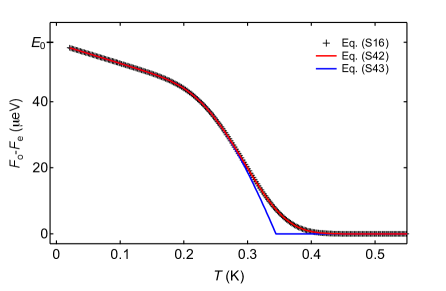
Fig. S4: Comparison of free energy approximations. Free energy difference $F_{\mathrm{o}}-F_{\mathrm{e}}$ versus temperature $T$ for three different expressions for the free energy. All parameters same as main text ($\Delta=180~{}\mathrm{\mu eV}$, $E_{0}=58~{}\mathrm{\mu eV}$, $\gamma=0$, $B=0$). Black crosses are numerically exact values from Eq. (S16), red line is Eq. (S42), blue line is Eq. (S43).

Equations (S42) and (S43) constitute two levels of accuracy at which Eq. (S16) can be evaluated. Figure S4 compares the methods. Equation (S42) is an excellent approximation to Eq. (S16) over the experimentally relevant temperature range. Equation (S43) is poor approximation at intermediate temperatures.

II.6 6. Effect of the bound state on the free energy

Figure S5 shows a comparison of the free energy difference, $F_{\mathrm{o}}-F_{\mathrm{}}$, with and without the subgap bound state. As the lowest energy unoccupied state, the bound state causes the free energy to saturate at $F_{\mathrm{o}}-F_{\mathrm{e}}=E_{0}$ at low temperature. It should be noted that the free energy difference with a subgap bound state was also shown in Fig. 5 of Lafarge et al. Lafarge et al. (1993).

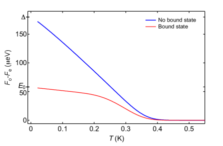
Fig. S5: Effect of bound state on free energy. Free energy difference $F_{\mathrm{o}}-F_{\mathrm{e}}$ versus temperature $T$ with and without the semiconductor bound state. All parameters the same as main text ($\Delta=180~{}\mathrm{\mu eV}$, $E_{0}=58~{}\mathrm{\mu eV}$, $\gamma=0$, $B=0$). Blue trace includes the BCS density of states only, red trace includes the BCS density of states and the discrete state.

References

(1)
Lang, K. M., Nam, S.,
Aumentado, J., Urbina, C. &
Martinis, J. M.
Banishing quasiparticles from Josephson-junction
qubits: Why and how to do it.
Applied Superconductivity, IEEE Transactions
on13, 989–993
(2003).
(2)
Aumentado, J., Keller, M. W.,
Martinis, J. M. & Devoret, M. H.
Nonequilibrium quasiparticles and periodicity
in single-Cooper-pair transistors.
Physical Review Letters92, 066802
(2004).
(3)
Martinis, J. M., Ansmann, M. &
Aumentado, J.
Energy decay in superconducting Josephson-junction
qubits from nonequilibrium quasiparticle excitations.
Physical Review Letters103, 097002
(2009).
(4)
De Visser, P. J. et al.Number fluctuations of sparse quasiparticles in a
superconductor.
Physical Review Letters106 (2011).
(5)
Saira, O. P., Kemppinen, A.,
Maisi, V. F. & Pekola, J. P.
Vanishing quasiparticle density in a hybrid Al/Cu/Al
single-electron transistor.
Physical Review B85, 012504
(2012).
(6)
Pop, I. M. et al.Coherent suppression of electromagnetic dissipation
due to superconducting quasiparticles.
Nature508,
369–372 (2014).
(7)
Leijnse, M. & Flensberg, K.
Scheme to measure Majorana fermion lifetimes using a
quantum dot.
Physical Review B84, 140501
(2011).
(8)
Rainis, D. & Loss, D.
Majorana qubit decoherence by quasiparticle
poisoning.
Physical Review B85, 174533
(2012).
(9)
Cheng, M., Lutchyn, R. M. &
Das Sarma, S.
Topological protection of Majorana qubits.
Physical Review B85, 165124
(2012).
(10)
Ferguson, A., Court, N.,
Hudson, F. & Clark, R.
Microsecond resolution of quasiparticle tunneling in
the single-Cooper-pair transistor.
Physical Review Letters97, 106603
(2006).
(11)
Zgirski, M. et al.Evidence for long-Lived quasiparticles trapped in
superconducting point contacts.
Physical Review Letters106, 257003
(2011).
(12)
Sun, L. et al.Measurements of Quasiparticle Tunneling Dynamics in
a Band-Gap-Engineered Transmon Qubit.
Physical Review Letters108, 230509
(2012).
(13)
Ristè, D. et al.Millisecond charge-parity fluctuations and induced
decoherence in a superconducting transmon qubit.
Nature Communications4, 1913 (2013).
(14)
Maisi, V. F. et al.Excitation of single quasiparticles in a small
superconducting Al island connected to normal-Metal leads by tunnel
junctions.
Physical Review Letters111, 147001
(2013).
(15)
Doh, Y. J. et al.Tunable supercurrent through semiconductor
nanowires.
Science309,
272–275 (2005).
(16)
Hofstetter, L., Csonka, S.,
Nygård, J. & Schönenberger, C.
Cooper pair splitter realized in a two-quantum-dot
Y-junction.
Nature461,
960–963 (2009).
(17)
Pillet, J.-D. et al.Andreev bound states in supercurrent-carrying carbon
nanotubes revealed.
Nature Physics6, 965–969
(2010).
(18)
De Franceschi, S., Kouwenhoven, L.,
Schoenenberger, C. & Wernsdorfer, W.
Hybrid superconductor-quantum dot devices.
Nature Nanotechnology5, 703–711
(2010).
(19)
Giazotto, F. et al.A Josephson quantum electron pump.
Nature Physics7, 857–861
(2011).
(20)
Sau, J. D., Lutchyn, R. M.,
Tewari, S. & Das Sarma, S.
Generic new platform for topological quantum
computation using semiconductor heterostructures.
Physical Review Letters104, 040502
(2010).
(21)
Lutchyn, R. M., Sau, J. D. &
Das Sarma, S.
Majorana fermions and a topological phase transition
in semiconductor-superconductor heterostructures.
Physical Review Letters105, 077001
(2010).
(22)
Oreg, Y., Refael, G. &
von Oppen, F.
Helical liquids and majorana bound states in quantum
wires.
Physical Review Letters105, 177002
(2010).
(23)
Padurariu, C. & Nazarov, Y. V.
Theoretical proposal for superconducting spin
qubits.
Physical Review B81, 144519
(2010).
(24)
Leijnse, M. & Flensberg, K.
Coupling spin qubits via superconductors.
Physical Review Letters111, 060501
(2013).
(25)
Mourik, V. et al.Signatures of Majorana fermions in hybrid
superconductor-semiconductor nanowire devices.
Science336,
1003–1007 (2012).
(26)
Das, A. et al.Zero-bias peaks and splitting in an
Al–InAs nanowire topological superconductor as a signature of
Majorana fermions.
Nature Physics8, 887–895
(2012).
(27)
Deng, M. T. et al.Anomalous zero-bias conductance peak in a
Nb–InSb nanowire–Nb hybrid device.
Nano Letters12,
6414–6419 (2012).
(28)
Churchill, H. O. H. et al.Superconductor-nanowire devices from tunneling to
the multichannel regime: Zero-bias oscillations and magnetoconductance
crossover.
Physical Review B87, 241401
(2013).
(29)
Deacon, R. S. et al.Tunneling spectroscopy of Andreev energy levels in a
quantum dot coupled to a superconductor.
Physical Review Letters104, 076805
(2010).
(30)
Lee, E. J. H. et al.Zero-bias anomaly in a nanowire quantum dot coupled
to superconductors.
Physical Review Letters109, 186802
(2012).
(31)
Lee, E. J. H. et al.Spin-resolved Andreev levels and parity crossings in
hybrid superconductor–semiconductor nanostructures.
Nature Nanotechnology9, 79–84 (2014).
(32)
Chang, W., Manucharyan, V. E.,
Jespersen, T. S., Nygård, J. &
Marcus, C. M.
Tunneling spectroscopy of quasiparticle bound states
in a spinful Josephson junction.
Physical Review Letters110, 217005
(2013).
(33)
Sau, J. D. & Das Sarma, S.
Realizing a robust practical Majorana chain in a
quantum-dot-superconductor linear array.
Nature Communications3, 964 (2012).
(34)
Leijnse, M. & Flensberg, K.
Parity qubits and poor man’s Majorana bound states
in double quantum dots.
Physical Review B86, 134528
(2012).
(35)
Fulga, I. C., Haim, A.,
Akhmerov, A. R. & Oreg, Y.
Adaptive tuning of Majorana fermions in a quantum
dot chain.
New Journal of Physics15, 045020
(2013).
(36)
Fu, L.
Electron teleportation via Majorana bound states in
a mesoscopic superconductor.
Physical Review Letters104, 056402
(2010).
(37)
Hützen, R., Zazunov, A.,
Braunecker, B., Yeyati, A. L. &
Egger, R.
Majorana single-charge transistor.
Physical Review Letters109, 166403
(2012).
(38)
Krogstrup, P. et al.Epitaxy of semiconductor–superconductor
nanowires.
Nature Materials AOP
(2015).
(39)
Chang, W. et al.Hard gap in epitaxial
semiconductor–superconductor nanowires.
Nature Nanotechnology
(2015).
(40)
Tuominen, M. T., Hergenrother, J. M.,
Tighe, T. S. & Tinkham, M.
Experimental evidence for parity-based 2e
periodicity in a superconducting single-electron tunneling transistor.
Physical Review Letters69, 1997 (1992).
(41)
Lafarge, P., Joyez, P.,
Esteve, D., Urbina, C. &
Devoret, M. H.
Measurement of the even-odd free-energy difference
of an isolated superconductor.
Physical Review Letters70, 994–997
(1993).
(42)
Averin, D. V. & Nazarov, Y. V.
Single-electron charging of a superconducting
island.
Physical Review Letters69, 1993–1996
(1992).
(43)
Matveev, K. A., Glazman, L. I. &
Shekhter, R. I.
Effects of charge parity in tunneling through a
superconducting grain.
Modern Physics Letters08, 1007–1026
(1994).
(44)
Hekking, F. W. J., Glazman, L. I.,
Matveev, K. A. & Shekhter, R. I.
Coulomb blockade of two-electron tunneling.
Physical Review Letters70, 4138–4141
(1993).
(45)
Hergenrother, J. M., Tuominen, M. T. &
Tinkham, M.
Charge transport by Andreev reflection through a
mesoscopic superconducting island.
Physical Review Letters72, 1742–1745
(1994).
(46)
Aleiner, I. L., Brouwer, P. W. &
Glazman, L. I.
Quantum effects in Coulomb blockade.
Physics Reports358, 309–440
(2002).
(47)
Björk, M. T. et al.Tunable effective factor in InAs nanowire
quantum dots.
Physical Review B72, 201307
(2005).
(48)
Csonka, S. et al.Giant fluctuations and gate control of the
-factor in InAs nanowire quantum dots.
Nano Letters8,
3932–3935 (2008).
(49)
Olivares, D. G. et al.Dynamics of quasiparticle trapping in Andreev
levels.
Physical Review B89, 104504
(2014).
(50)
Zazunov, A., Brunetti, A.,
Yeyati, A. L. & Egger, R.
Quasiparticle trapping, Andreev level population
dynamics, and charge imbalance in superconducting weak links.
Physical Review B90, 104508
(2014).