On the large time behavior of the solutions of a nonlocal ordinary differential equation with mass conservation

Abstract. We consider an initial value problem for a nonlocal differential equation with a bistable nonlinearity in several space dimensions. The equation is an ordinary differential equation with respect to the time variable $t$, while the nonlocal term is expressed in terms of spatial integration. We discuss the large time behavior of solutions and prove, among other things, the convergence to steady-states. The proof that the solution orbits are relatively compact is based upon the rearrangement theory.

1 Introduction

1.1 Motivation

In this paper, we study solutions $u(x,t)$ of the initial value problem

$$(P)\ \ \left\{\begin{array}[]{ll}u_{t}=f(u)-\langle f(u)\rangle&x\in\Omega,\,t>0,\vspace{6pt}\\ u(x,0)=u_{0}(x)&x\in\Omega,\end{array}\right.$$

where $\Omega$ is a bounded open set in ${\mathbb{R}}^{N}$ with $N\geq 1$ and

$$\langle f(u)\rangle:=\frac{1}{|\Omega|}\int_{\Omega}f(u(x,t))\,dx.$$

Here $|A|$ denotes the Lebesgue measure of a set $A\subset\Omega$, $u_{0}$ is a bounded function on $\Omega$ and $f(u)$ is a bistable nonlinearity. More precise conditions on $f$ will be specified later. A typical example is $f(u)=u-u^{3}$. Note that the Problem $(P)$ does not change if we replace $f$ by $f+c$ where $c$ is any constant.

Solutions of Problem $(P)$ satisfy the following mass conservation property

$$\int_{\Omega}u(x,t)\,dx=\int_{\Omega}u_{0}(x)\,dx\mbox{~{}~{}for all~{}~{}}t\geq 0.$$ (1)

This is easily seen by integrating the equation in $(P)$, but we will state it more precisely in Theorem 1.1. Note also that Problem $(P)$ formally represents a gradient flow for the functional

$$E(u)=-\int_{\Omega}F(u)\mbox{~{}~{}with~{}~{}}F(s)=\int_{0}^{s}f(\sigma)\,d\sigma$$ (2)

on the space $X:=\{w\in L^{2}(\Omega):\int_{\Omega}w\,dx=\int_{\Omega}u_{0}\,dx\}$ (see Remark 4.2).

Let us explain the motivation of the present work briefly. The singular limit of reaction-diffusion equations, in particular, the generation of interface and the motion of interface have been studied by many authors, for instance [1], [4], [5]. This paper is motivated by the study of a generation of interface property for the Allen-Cahn equation with mass conservation:

$$(P^{\varepsilon})\ \ \left\{\begin{array}[]{ll}u^{\varepsilon}_{t}=\Delta u^{\varepsilon}+\dfrac{1}{\varepsilon^{2}}(f(u^{\varepsilon})-\langle f(u^{\varepsilon})\rangle)&\mbox{in }\Omega\times(0,\infty),\vspace{5pt}\\ \dfrac{\partial u^{\varepsilon}}{\partial\nu}=0&\mbox{on }\partial\Omega\times(0,\infty),\vspace{8pt}\\ u^{\varepsilon}(x,0)=u_{0}(x)&x\in\Omega.\end{array}\right.$$

We refer the reader to [12] for the motivation of studying this model.

If we use a new time scale $\tau:=t/\varepsilon^{2}$ in order to study the behavior of the solution at a very early stage, then the equation in $(P^{\varepsilon})$ is rewritten as follows:

$$u^{\varepsilon}_{\tau}=\varepsilon^{2}\Delta u^{\varepsilon}+f(u^{\varepsilon})-\langle f(u^{\varepsilon})\rangle.$$ (3)

If the term $\varepsilon^{2}\Delta u^{\varepsilon}$ is negligible for sufficiently small $\varepsilon$, then (3) reduces to the equation in $(P)$, thus one can expect that $(P)$ is a good approximation of $(P^{\varepsilon})$ in the time scale $\tau$ so long as $\varepsilon^{2}\Delta u^{\varepsilon}$ is negligible.

In the standard Allen-Cahn problem $u^{\varepsilon}_{t}=\Delta u^{\varepsilon}+\dfrac{1}{\varepsilon^{2}}f(u^{\varepsilon})$, it is known that the term $\varepsilon^{2}\Delta u^{\varepsilon}$ is indeed negligible for a rather long time span of $\tau=O(|\ln\varepsilon|)$, or equivalently $t=O(\varepsilon^{2}|\ln\varepsilon|)$. During this period, the solution typically develops steep transition layers (generation of interface). After that, the term $\varepsilon^{2}\Delta u^{\varepsilon}$ is no longer negligible; see, for example, [1, 4] for details.

It turns out that the same is true of Problem $(P^{\varepsilon})$, as we will show in our forthcoming paper [8]. In other words, $(P^{\varepsilon})$ is well approximated by the ordinary differential equation $(P)$ for a rather long time span in $\tau$. Thus, in order to analyze the behavior of solutions of $(P^{\varepsilon})$ at the very early stage, it is important to understand the large time behavior of solutions of $(P)$.

We will show in this paper that the solution of $(P)$ converges to a stationary solution as $t\to\infty$. Furthermore, in many cases the limit stationary solutions are step functions that take two values $a_{-}$ and $a_{+}$ which satisfy

$$f(a_{-})=f(a_{+}),\quad f^{\prime}(a_{-})<0,\quad f^{\prime}(a_{+})<0.$$

Consequently, one may expect that, at the very early stage, the solution $u^{\varepsilon}$ to Problem $(P^{\varepsilon})$ typically approaches a configuration consisting of plateaus near the values $a_{-}$ and $a_{+}$ and steep interfaces (transition layers) connecting the regions $\{x\in\Omega:u^{\varepsilon}\approx a_{-}\}$ and $\{x\in\Omega:u^{\varepsilon}\approx a_{+}\}$. In order to make this conjecture rigorous, one needs a more precise error estimate between $(P)$ and $(P^{\varepsilon})$, which will be given in the above-mentioned forthcoming article [8].

1.2 Main results

Before stating our main results, let us specify our assumptions on the nonlinearity $f$. For the most part we will consider a bistable nonlinearity satisfying $\bf(F_{1}),(F_{2})$ below, but some of our results hold under a milder condition $\bf(F^{\prime})$, which allows $f$ to be a multi-stable or a more general nonlinearity.

• $f\in C^{1}({\mathbb{R}})$, and there exist $m<M$ satisfying $f^{\prime}(m)=f^{\prime}(M)=0$ and

  $$f^{\prime}<0\mbox{~{}~{}on~{}~{}}(-\infty,m)\cup(M,\infty),\quad f^{\prime}>0\mbox{~{}~{}on~{}~{}}(m,M).$$

• There exist $s_{*}<s^{*}$ satisfying

  $$\begin{cases}s_{*}<m<M<s^{*},\\ f(s_{*})=f(M),\quad f(s^{*})=f(m).\end{cases}$$ (4)

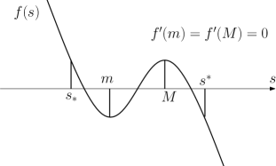
Figure 1: Bistable nonlinearity

A milder version of our assumption is the following. This assumption allows $f$ to be a multistable nonlinearity. Any periodic nonlinearity such as $f(s)=\sin s$ also satisfies this milder assumption.

• $f:{\mathbb{R}}\to{\mathbb{R}}$ is locally Lipschitz continuous and there exist two sequences $\{a_{n}\}$, $\{b_{n}\}$, with $a_{n}\leq b_{n}$, such that $a_{n}\to-\infty$, $b_{n}\to\infty$ as $n\to\infty$ and that

  $$f(a_{n})\geq f(s)\geq f(b_{n})\mbox{~{}~{}for all~{}~{}}s\in[a_{n},b_{n}].$$

Clearly $\bf(F_{1})$, $\bf(F_{2})$ imply $\bf(F^{\prime})$. The assumption $\bf(F^{\prime})$ will be used only in Theorem 1.4 below. Unless otherwise stated, we will always assume $\bf(F_{1}),(F_{2})$.

In Theorems 1.1 and 1.3 below we present existence and uniqueness results for the solution of Problem $(P)$ and give basic properties of the $\omega$-limit set under the assumption that $u_{0}\in L^{\infty}(\Omega)$. Note that we will henceforth regard $(P)$ as an ordinary differential equation on $L^{\infty}(\Omega)$. More precisely, $u$ is a solution on the interval $0\leq t<T$ if $u\in C^{1}([0,T);L^{\infty}(\Omega))$ and satisfies

$$(P^{\prime})\ \ \left\{\begin{array}[]{ll}\dfrac{du}{dt}=H(u)&t>0,\vspace{6pt}\\ u(0)=u_{0},\end{array}\right.$$

where $H:L^{\infty}(\Omega)\to L^{\infty}(\Omega)$ is defined by

$$H(u):=f(u)-\langle f(u)\rangle.$$ (5)

As we will see later in (12), Problem $(P^{\prime})$ is equivalent (a.e. in $\Omega$) to the original Problem $(P)$, which is considered pointwise for each $x\in\Omega.$ We will abbreviate $u(x,t)$ as $u(t)$ when we regard $u$ as an $L^{\infty}(\Omega)$-valued function. We may mix the two notations so long as there is no fear of confusion.

For any $u_{0}\in L^{\infty}(\Omega)$, we fix two constants $s_{1}<s_{2}$ such that

$$s_{1},s_{2}\not\in(s_{*},s^{*})$$

and that

$$s_{1}\leq u_{0}(x)\leq s_{2}\mbox{~{}~{}for a.e.~{}~{}}x\in\Omega.$$

For example, if we set

$$\alpha:=\operatorname{ess\,inf}_{x\in\Omega}u_{0}(x),\quad\beta:=\operatorname{ess\,sup}_{x\in\Omega}u_{0}(x),$$ (6)

then $s_{1},s_{2}$ can be chosen as follows:

$$\begin{cases}[\alpha,\beta]\cap(s_{*},s^{*})=\varnothing\quad\Rightarrow\quad s_{1}:=\alpha,s_{2}:=\beta,\\ [\alpha,\beta]\cap(s_{*},s^{*})\neq\varnothing\quad\Rightarrow\quad s_{1}=\min\{\alpha,s_{*}\},s_{2}=\max\{\beta,s^{*}\}.\end{cases}$$

For later reference we summarize the above hypotheses as follows:

$\bf(H)$ $s_{1},s_{2}\not\in(s_{*},s^{*})$   and   $s_{1}\leq u_{0}(x)\leq s_{2}\mbox{~{}~{}for a.e.~{}~{}}x\in\Omega.~{}$

Theorem 1.1.

Assume that $u_{0}\in L^{\infty}(\Omega)$ and let $s_{1},s_{2}$ be as in $\bf(H)$. Then Problem $(P)$ possesses a unique time-global solution $u\in C^{1}([0,\infty);L^{\infty}(\Omega))$. Moreover, the solution has the mass conservation property (1)and, for all $t\geq 0$,

$$s_{1}\leq u(x,t)\leq s_{2}\mbox{~{}~{}~{}for a.e.~{}~{}}x\in\Omega.$$ (7)

The next theorem is concerned with the structure of the $\omega$-limit set. Here the $\omega$-limit set of a solution $u(t)$ of $(P)$ (or more precisely $(P^{\prime})$) with initial data $u_{0}$ is defined as follows:

Definition 1.2.

We define the $\omega$-limit set of $u_{0}$ by

$$\omega(u_{0}):=\{\varphi\in L^{1}(\Omega):\exists t_{n}\to\infty,u(t_{n})\to\varphi\mbox{~{}~{}in~{}~{}}L^{1}(\Omega)\mbox{~{}as~{}}n\to\infty\}.$$

The reason why we use the topology of $L^{1}(\Omega)$, not $L^{\infty}(\Omega)$, to define the $\omega$-limit set is that the solution often develops sharp transition layers which cannot be captured by the $L^{\infty}(\Omega)$ topology. Note that, since the solution $u$ is uniformly bounded in $L^{\infty}(\Omega)$ by (7), the topology of $L^{p}(\Omega)$ is equivalent to that of $L^{1}(\Omega)$ for all $p\in[1,\infty)$.

Theorem 1.3.

Let $u_{0},s_{1},s_{2}$ be as in Theorem 1.1. Then

1. $\omega(u_{0})$ is a nonempty compact connected set in $L^{1}(\Omega)$.

2. Any element $\varphi\in\omega(u_{0})$ satisfies $s_{1}\leq\varphi\leq s_{2}$ a.e. and is a stationary solution of $(P)$. More precisely, it satisfies

   $$f(\varphi(x))-\langle f(\varphi)\rangle=0\mbox{~{}~{}~{}for a.e.~{}~{}}x\in\Omega.$$

Note that the constant $\langle f(\varphi)\rangle$ that appears in the above equation is not specified a priori. It depends on each $\varphi$. This is in marked contrast with the standard Allen-Cahn problem, in which stationary solutions are defined by the equation $f(\varphi)=0.$

The next theorem is a generalization of Theorems 1.1 and 1.3 to a larger class of nonlinearities including multi-stable ones. In this theorem (and only here) we assume $(\bf F^{\prime})$ instead of $\bf(F_{1}),(F_{2})$.

Theorem 1.4 (The case of multi-stable nonlinearity).

Assume $\bf(F^{\prime})$ and let $u_{0}\in L^{\infty}(\Omega)$. Choose $n\in{\mathbb{N}}$ such that $a_{n}\leq u_{0}(x)\leq b_{n}\;a.e.\;x\in\Omega$. Then Problem $(P)$ possesses a unique time-global solution $u\in C^{1}([0,\infty);L^{\infty}(\Omega))$. The solution satisfies (1) and, for each $t\geq 0$,

$$a_{n}\leq u(x,t)\leq b_{n}\mbox{~{}~{}for a.e.~{}~{}}x\in\Omega.$$

Furthermore, the conclusions of Theorem 1.3 hold with $s_{1},s_{2}$ replaced by $a_{n},b_{n}$, respectively.

The following two theorems are concerned with the fine structure of the $\omega$-limit sets under the assumptions $\bf(F_{1}),(F_{2})$.

Theorem 1.5.

Let $u_{0}\in L^{\infty}(\Omega)$ satisfy $\langle u_{0}\rangle\not\in[s_{*},s^{*}]$. Then $\omega(u_{0})$ has a unique element $\varphi$ which is given by

$$\varphi=\langle u_{0}\rangle.$$

Moreover, there exist constants $C_{1},C_{2}>0$ such that

$$\|u(t)-\langle u_{0}\rangle\|_{L^{\infty}(\Omega)}\leq C_{1}\exp(-C_{2}t)\mbox{~{}~{}for all~{}~{}}t\geq 0.$$ (8)

Theorem 1.6.

Let $u_{0}\in L^{\infty}(\Omega)$ satisfy $s_{*}\leq\langle u_{0}\rangle\leq s^{*}$. Assume that

$$|\{x:u_{0}(x)=s\}|=0\mbox{~{}~{}for all~{}~{}}s\in{\mathbb{R}}.$$ (9)

Then $\omega(u_{0})$ contains only one element $\varphi$ and it is a step function that takes at most two values. More precisely one of the following holds:

1. there exist $a_{-},a_{+}$ with $s_{*}<a_{-}<m,M<a_{+}<s^{*},f(a_{-})=f(a_{+})$ and disjoint subsets $\Omega_{-},\Omega_{+}\subset\Omega$ with $\Omega_{-}\cup\Omega_{+}=\Omega$ satisfying

   $$\varphi(x)=a_{-}\chi_{\Omega_{-}}(x)+a_{+}\chi_{\Omega_{+}}(x)\mbox{~{}~{}for a.e.~{}~{}}x\in\Omega,$$

   where $\chi_{A}(x)$ denotes the characteristic function of a set $A\subset\Omega$;

2. $\varphi(x)\in\{m,s^{*}\}\mbox{~{}~{}for a.e.~{}~{}}x\in\Omega$;

3. $\varphi(x)\in\{s_{*},M\}\mbox{~{}~{}for a.e.~{}~{}}x\in\Omega$.

Remark 1.7.

If $\omega(u_{0})$ contains only one element $\varphi$, then for all $p\in[1,\infty)$,

$$u(t)\to\varphi\mbox{~{}~{}in~{}~{}}L^{p}(\Omega)\mbox{~{}~{}as~{}~{}}t\to\infty.$$

The proof of Theorem 1.6 is presented in two steps. First we consider the special case where $u_{0}$ satisfies the following pointwise inequalities:

$$s_{*}\leq u_{0}(x)\leq s^{*}\mbox{~{}~{}for a.e.~{}~{}}x\in\Omega,$$

and then prove the theorem for the general case. The results in the special case are stated in Theorem 6.5.

One of the difficulties of Problem $(P)$ is the presence of the nonlocal term $\langle f(u)\rangle$. Because of this term, we do not have the standard comparison principle for solutions of $(P)$, or $(P^{\prime})$. Another difficulty is due to the lack of diffusion term, so that the solution in general is not smooth at all in space. Furthermore, since the solution can develop many sharp transition layers at least in some cases, the solution does not necessarily remain bound in $BV(\Omega)$, which makes it difficult to prove the relative compactness of the solution even in $L^{1}(\Omega)$. This difficulty is overcome by considering the unidimensional equi-measurable rearrangement $u^{\sharp}$ and showing that it is a solution of a one-dimensional problem $(P^{\sharp})$ to be introduced in Subsection 3.2. Since the orbit $\{u^{\sharp}(t):t\geq 0\}$ is bounded in $BV(\Omega^{\sharp})$, where $\Omega^{\sharp}:=(0,|\Omega|)\subset{\mathbb{R}}$, it is relatively compact in $L^{1}(\Omega^{\sharp})$. We then prove that the convergence of $u^{\sharp}(t_{n})$ in $L^{1}(\Omega^{\sharp})$ is equivalent to the convergence of $u(t_{n})$ in $L^{1}(\Omega)$. These two facts establish the relative compactness of $\{u(t):t\geq 0\}$ in $L^{1}(\Omega)$.

As we will show in Section 4, Problem $(P)$ possesses a Lyapunov functional $E(u)$. This and the relative compactness of the solution orbit imply that the $\omega$-limit set of the solution is nonempty and consists only of stationary solutions of ${(P)}$. However, another difficulty of Problem $(P)$ is that there are too many (actually a continuum) of stationary solutions. This makes it difficult to find a good characterization of the $\omega$-limit set of solutions. This difficulty will be overcome by careful observation of the dynamics of solutions near the unstable zero of the function $f(s)-\langle f(u(\cdot,t))\rangle$.

The paper is organized as follows: In Section 2, we prove the existence and uniqueness of the solution of $(P)$ and prove Theorem 1.1. In Section 3, using the monotone rearrangement theory, we introduce the one-dimensional problem $(P^{\sharp})$ and study the relation between the behavior of solutions of $(P)$ and that of $(P^{\sharp})$, which is an essential ingredient for proving Theorem 1.3 (i). In Section 4, we prove Theorem 1.3 (ii) by using the Lyapunov functional $E(u)$. We also prove Theorem 1.4 for multi-stable nonlinearity in this section. In Section 5, we prove Theorem 1.5. Finally, in Section 6, we prove Theorem 1.6.

2 Proof of Theorem 1.1

In this section we prove the global existence and uniqueness of solutions of $(P)$ (or more precisely $(P^{\prime})$), which will be done in two steps. In Subsection 2.1, we only assume that $f$ is locally Lipschitz continuous and prove the existence of a local-in-time solution as well as its uniqueness. This result is an immediate consequence of the local Lipschitz continuity of the nonlocal nonlinear term in the space $L^{\infty}(\Omega)$. Then, in Subsection 2.2, with an additional assumption, we prove the uniform boundedness of the solution, which implies the global existence. Finally in Subsection 2.3, we apply the results of Subsections 2.1 and 2.2 to prove Theorem 1.1.

2.1 Local existence and uniqueness

In this subsection, we always assume that $f:{\mathbb{R}}\to{\mathbb{R}}$ is locally Lipschitz continuous.

Lemma 2.1.

Assume that $f$ is locally Lipschitz continuous. Then for each $u_{0}\in L^{\infty}(\Omega)$, $(P^{\prime})$ has a unique local-in-time solution.

Proof.

Since $f:{\mathbb{R}}\to{\mathbb{R}}$ is locally Lipschitz continuous, the Nemytskii operator $u\mapsto f(u)$ is clearly locally Lipschitz in $L^{\infty}(\Omega)$. Therefore $u\mapsto\langle f(u)\rangle$ is also locally Lipschitz since $\Omega$ is bounded. It follows that the map $H:L^{\infty}(\Omega)\to L^{\infty}(\Omega)$ defined in (5) is locally Lipschitz continuous. Hence the assertion of the lemma follows from the standard theory of ordinary differential equations. ∎

Denote by $[0,T_{max}(u_{0}))$, with $0<T_{max}(u_{0})\leq\infty$, the maximal time interval for the existence of the solution of $(P^{\prime})$ with initial data $u_{0}$. Then the following lemma also follows from the standard theory of ordinary differential equations.

Lemma 2.2.

Let $u\in C^{1}([0,T_{max}(u_{0}));L^{\infty}(\Omega))$ be the solution of $(P^{\prime})$ with $u_{0}\in L^{\infty}(\Omega)$. If $T_{max}(u_{0})<\infty$, then

$$\limsup_{t\uparrow T_{max}(u_{0})}\|u(t)\|_{L^{\infty}(\Omega)}=\infty.$$

Corollary 2.3.

If there exists $C>0$ such that

$$\|u(t)\|_{L^{\infty}(\Omega)}\leq C\mbox{~{}~{}for all~{}~{}}t\in[0,T_{max}(u_{0})),$$

then $T_{max}(u_{0})=\infty$.

2.2 Uniform bounds and global existence

In this subsection, we continue to assume that $f$ is locally Lipschitz continuous. We fix $u_{0}\in L^{\infty}(\Omega)$ arbitrarily, and write $T_{max}$ instead of $T_{max}(u_{0})$ for simplicity. Set

$$\lambda(t)=\langle f(u(t))\rangle\mbox{~{}~{}for all~{}~{}}t\in[0,T_{max}),$$ (10)

and study solutions $Y(t;s)$ of the following auxiliary problem:

$$(ODE)\,\,\begin{cases}\dot{Y}=f(Y)-\lambda(t),\quad t>0,\vspace{6pt}\\ Y(0)=s,\end{cases}$$ (11)

where $\dot{Y}:=dY/dt$. Since $u\in C^{1}([0,T_{max});L^{\infty}(\Omega))$, it is easy to see that there exits a function $u^{*}:\Omega\times[0,T_{max})\to{\mathbb{R}}$ satisfying for all $t\in[0,T_{max})$

$$u^{*}(x,t)=u(x,t)\mbox{~{}~{}for a.e.~{}~{}}x\in\Omega,$$

and

$$\dfrac{\partial u^{*}}{\partial t}(x,t)=f(u^{*}(x,t))-\lambda(t)\mbox{~{}~{}for a.e.~{}~{}}x\in\Omega\mbox{~{}~{}and for all~{}~{}}t\in[0,T_{max}).$$

Consequently, for all $t\in[0,T_{max})$,

$$u(x,t)=Y(t;u_{0}(x))\mbox{~{}~{}for a.e.~{}~{}}x\in\Omega.$$ (12)

The lemma below proves the monotonicity of $Y(t;s)$ in $s$.

Lemma 2.4.

Let $\widetilde{s}<s$ and let $0<T<T_{max}$. Assume that Problem $(ODE)$ with initial conditions $\widetilde{s},s$ possesses the solutions $Y(t;\widetilde{s}),Y(t;s)\in C^{1}([0,T])$, respectively. Then

$$Y(t;\widetilde{s})<Y(t;s)\mbox{~{}~{}for all~{}~{}}t\in[0,T].$$ (13)

Proof.

Since $Y(0;\widetilde{s})=\widetilde{s}<s=Y(0;s)$, the assertion follows immediately from the backward uniqueness of solution of $(ODE)$. ∎

Lemma 2.5.

Let $f:{\mathbb{R}}\to{\mathbb{R}}$ be a locally Lipschitz function and let $u$ be the solution of $(P^{\prime})$ with initial data $u_{0}\in L^{\infty}(\Omega)$. Assume that there exist $a\leq b$ such that

$$f(a)\geq f(s)\geq f(b)\ \ \hbox{for}\ \ s\in[a,b]$$ (14)

and that

$$a\leq u_{0}(x)\leq b\quad\hbox{for}\ \ a.e.\ \ x\in\Omega.$$ (15)

Then the solution $u$ exists globally for $t\geq 0$ and it satisfies, for every $t\geq 0$,

$$a\leq u(x,t)\leq b\quad\hbox{for}\ \ a.e.\ \ x\in\Omega.$$ (16)

Proof.

We will show that (16) holds so long as the solution $u$ exists. The global existence will then follow automatically from the local existence result in Subsection 2.1. Let $Y(t,s)$ be the solution of (ODE). The assumption (15) and the monotonicity of $Y(t;s)$ in $s$ imply

$$Y(t;a)\leq Y(t;u_{0}(x))=u(x,t)\leq Y(t;b)\quad\ a.e.\ \ x\in\Omega.$$

Therefore, in order to prove (16), it suffices to show that

$$a\leq Y(t;a),\quad\ Y(t;b)\leq b$$ (17)

so long as the solutions $Y(t;a),Y(t;b)$ both exist.

We first consider the special case where $f$ satisfies

$$f(s)=f(a)\ \ \hbox{for}\ \ s\in(-\infty,a],\quad f(s)=f(b)\ \ \hbox{for}\ \ s\in[b,\infty).$$ (18)

Then we have $f(s)\geq f(\tilde{s})$ for any $s\in{\mathbb{R}}$ and $\tilde{s}\geq b$. It follows that $f(Y(t;u_{0}))\geq f(Y(t;b))\mbox{~{}~{}a.e. in~{}~{}}\Omega$ for every $t\geq 0$ such that $Y(t;b)\geq b$. Hence $\lambda(t)\geq f(Y(t;b))$ for every such $t$. Consequently,

$$\dot{Y}(t;b)=f(Y(t;b))-\lambda(t)\leq 0\ \ \hbox{for every $t$ such that}\ \ Y(t,b)\geq b.$$

This, together with $Y(0;b)=b$, proves the second inequality of (17). The first inequality of (17) can be shown similarly. This establishes (17), hence (16), under the additional assumption (18).

Next we consider the general case where (18) does not necessarily hold. Let $\tilde{f}:{\mathbb{R}}\to{\mathbb{R}}$ be defined by

$$\tilde{f}(s)=\begin{cases}f(a)&\mbox{~{}~{}for all~{}~{}}s<a,\\ f(s)&\hbox{~{}for}\ s\in[a,b],\\ f(b)&\mbox{~{}~{}for all~{}~{}}s>b,\end{cases}$$

and let $\tilde{u}(t)$ be the solution of the following problem:

$$\left\{\begin{array}[]{ll}\dfrac{d\tilde{u}}{dt}=\tilde{f}(\tilde{u})-\langle\tilde{f}(\tilde{u})\rangle&t>0,\vspace{6pt}\\ \tilde{u}(0)=u_{0}.\end{array}\right.$$

Then, by what we have shown above, the solution $\tilde{u}(t)$ exists globally for $t\geq 0$, and the following inequalities hold for every $t\geq 0$:

$$a\leq\tilde{u}(x,t)\leq b\quad\hbox{for}\ \ a.e.\ \ x\in\Omega.$$

Since $\tilde{f}(s)=f(s)$ for all $s\in[a,b]$, $\tilde{u}$ is also a solution of Problem $(P^{\prime})$, hence $\tilde{u}(x,t)=u(x,t)\;(a.e.\ x\in\Omega,\;t\geq 0)$ by the uniqueness of the solution of $(P^{\prime})$. This implies (16), and the proof of Lemma 2.5 is complete. ∎

The following corollary follows from the proof of Lemma 2.5.

Corollary 2.6.

Assume that all the hypotheses in Lemma 2.5 hold. Then for all $s\in[a,b]$, Problem $(ODE)$ has a unique solution $Y(t;s)\in C^{1}([0,\infty))$ and it satisfies

$$a\leq Y(t;s)\leq b\mbox{~{}~{}for all~{}~{}}s\in[a,b],\ t\geq 0.$$

2.3 Proof Theorem 1.1

Proof Theorem 1.1.

The local existence and uniqueness follow from Lemma 2.1. Let $s_{1},s_{2}$ be as in $\bf(H)$. We have

$$f(s_{1})\geq f(s)\geq f(s_{2})\mbox{~{}~{}for all~{}~{}}s\in[s_{1},s_{2}].$$

Set $a:=s_{1},b:=s_{2}$. Then the assertion (7) follows from Lemma 2.5. This and Corollary 2.3 imply global existence. Next we prove the mass conservation property (1). Integrating the equation in Problem $(P^{\prime})$ from $0$ to $t$, we obtain

$$u(t)-u(0)=\int_{0}^{t}u_{t}\,d\tau=\int_{0}^{t}[f(u)-\langle f(u)\rangle]\,d\tau,$$

so that

$$\int_{\Omega}u(x,t)\,dx-\int_{\Omega}u_{0}(x)\,dx=\int_{0}^{t}\int_{\Omega}[f(u)-\langle f(u)\rangle]\,dxd\tau=0.$$

This completes the proof of Theorem 1.1. ∎

Corollary 2.7.

Let $u$ be the solution of Problem $(P^{\prime})$ with $u_{0}\in L^{\infty}(\Omega)$ and let $t_{1}\geq 0$. Then

1. if $s_{*}\leq u(x,t_{1})\leq s^{*}$ for a.e. $x\in\Omega$, then for all $t\geq t_{1}$,

   $$s_{*}\leq u(x,t)\leq s^{*}\mbox{~{}~{}for a.e.~{}~{}}x\in\Omega;$$

2. if $u(x,t_{1})\leq s_{*}$ (resp. $u(x,t_{1})\geq s^{*}$) for a.e. $x\in\Omega$, then for all $t\geq t_{1}$,

   $$u(x,t)\leq s_{*}\quad(\mbox{resp.~{}~{}}u(x,t)\geq s^{*})\mbox{~{}~{}for a.e.~{}~{}}x\in\Omega.$$

Proof.

For (i), we simply set $s_{1}=s_{*},s_{2}=s^{*}$ and apply Theorem 1.1. For (ii) we set $s_{2}=s_{*}$ (resp. $s_{1}=s^{*}$). ∎

3 Proof of Theorem 1.3 (i)

This section is organized as follows: We first introduce the rearrangement theory in Subsection 3.1. Then in Subsection 3.2, we introduce Problem $(P^{\sharp})$ and study basic properties of its solutions which we state in Theorem 3.3. Finally, in Section 3.3, we prove the equivalence between the convergence of the solution $u(t)$ and its rearrangement $u^{\sharp}(t)$. This implies that the solution orbit $\{u(t):t\geq 0\}$ of $(P)$ is relatively compact in $L^{1}(\Omega)$, from which Theorem 1.3 (i) follows immediately.

3.1 Rearrangement theory

Given a measurable function $w:\Omega\to{\mathbb{R}}$, the distribution function of $w$ is defined by

$$\mu_{w}(\tau):=|\{x\in\Omega:w(x)>\tau\}|,\quad\tau\in{\mathbb{R}}.$$

Set

$$\Omega^{\sharp}:=(0,|\Omega|)\subset{\mathbb{R}}.$$

The unidimensional decreasing rearrangement of $w$, denoted $w^{\sharp}$, is defined on $\overline{\Omega^{\sharp}}=[0,|\Omega|]$ by

$$\begin{cases}&w^{\sharp}(0):=\operatorname{ess\,sup}(w),\vspace{6pt}\\ &w^{\sharp}(y)=\inf\{\tau:\mu_{w}(\tau)<y\},\quad y>0.\end{cases}$$ (19)

We recall some properties of $w^{\sharp}$ which are stated in [9, Chapter $1$].

Proposition 3.1.

The following properties hold:

1. $w^{\sharp}:\Omega^{\sharp}\to{\mathbb{R}}$ is nonincreasing and left-continuous.

2. $w,w^{\sharp}$ are equi-measurable, i.e. $\mu_{w}=\mu_{w^{\sharp}}$.

3. If $G$ is a Borel measurable function such that either $G\geq 0$ or $G(w)\in L^{1}(\Omega)$ then

   $$\int_{\Omega^{\sharp}}G(w^{\sharp}(y))\,dy=\int_{\Omega}G(w(x))\,dx.$$

4. Let $w_{1},w_{2}\in L^{p}(\Omega)$ with $1\leq p\leq\infty$; then

   $$\|w^{\sharp}_{1}-w^{\sharp}_{2}\|_{L^{p}(\Omega^{\sharp})}\leq\|w_{1}-w_{2}\|_{L^{p}(\Omega)}.$$

5. Let $\Phi:{\mathbb{R}}\to{\mathbb{R}}$ be nondecreasing. Then

   $$(\Phi(w))^{\sharp}(y)=\Phi(w^{\sharp}(y))\quad\mbox{~{}~{} for a.e.~{}~{}}y\in\Omega^{\sharp}.$$

Remark 3.2.

The function $w^{\sharp}$ is uniquely defined by the distribution function $\mu_{w}$. Moreover, by Proposition 3.1 (ii), if

$$s_{1}\leq w(x)\leq s_{2}\mbox{~{}~{}for a.e.~{}~{}}x\in\Omega,$$

then

$$s_{1}\leq w^{\sharp}(y)\leq s_{2}\mbox{~{}~{}for all~{}~{}}y\in\Omega^{\sharp}.$$

3.2 Associated one-dimensional problem $(P^{\sharp})$

Theorem 3.3.

Let $u(t)$ be the solution of Problem $(P^{\prime})$ with $u_{0}\in L^{\infty}(\Omega)$ and let $s_{1},s_{2}$ be as in $\bf(H)$. We define

$$u^{\sharp}(y,t):=(u(t))^{\sharp}(y)\mbox{~{}~{}on~{}~{}}\Omega^{\sharp}\times[0,\infty).$$ (20)

Then $u^{\sharp}$ is the unique solution in $C^{1}([0,\infty);L^{\infty}(\Omega^{\sharp}))$ of Problem $(P^{\sharp})$:

$$(P^{\sharp})\ \ \left\{\begin{array}[]{ll}\dfrac{dv}{dt}=f(v)-\langle f(v)\rangle,\quad t>0,\vspace{6pt}\\ v(0)=u_{0}^{\sharp}.\end{array}\right.$$

Moreover, for all $t\geq 0$,

$$s_{1}\leq u^{\sharp}(y,t)\leq s_{2}\mbox{~{}~{}for all~{}~{}}y\in\Omega^{\sharp},$$

and

$$u^{\sharp}(y,t)=Y(t;u_{0}^{\sharp}(y))\mbox{~{}~{}for a.e.~{}~{}}y\in\Omega^{\sharp}.$$ (21)

Proof.

In view of (12), we have for all $t\geq 0$,

$$u(x,t)=Y(t;u_{0}(x))\mbox{~{}~{}for a.e.~{}~{}}x\in\Omega.$$

Hence, since $Y(t;s)$ is increasing in $s$ (cf. Lemma 2.4), it follows from Proposition 3.1 (v) that for all $t\geq 0$,

$$u^{\sharp}(t)=Y(t;u^{\sharp}_{0})\mbox{~{}~{}a.e. in~{}~{}}\Omega^{\sharp}.$$ (22)

Moreover, (7) and Remark 3.2 imply that

$$s_{1}\leq u^{\sharp}(y,t)\leq s_{2}\mbox{~{}~{}for all~{}~{}}y\in\Omega^{\sharp},t\geq 0.$$ (23)

It remains to prove that $u^{\sharp}$ is the unique solution of Problem $(P^{\sharp})$. Since $Y(t;s)$ is the solution of Problem $(ODE)$, it follows that for all $t\geq 0$,

$$\frac{\partial Y}{\partial t}(t;u^{\sharp}_{0}) =f(Y(t;u^{\sharp}_{0}))-\lambda(t)$$

$$=f(u^{\sharp}(t))-\langle f(u(t))\rangle$$

$$=f(u^{\sharp}(t))-\langle f(u^{\sharp}(t))\rangle\quad\mbox{~{}~{}a.e. in~{}~{}}\Omega^{\sharp}.$$

Here we have used (22) and Proposition 3.1 (iii). Since the right-hand-side of the above equation is continuous in $t$ as an $L^{\infty}(\Omega)$-valued function, we have $u^{\sharp}=Y(\cdot,u^{\sharp}_{0}(\cdot))\in C^{1}([0,\infty);L^{\infty}(\Omega^{\sharp}))$. Hence $u^{\sharp}$ is a solution of Problem $(P^{\sharp})$ in $C^{1}([0,\infty);L^{\infty}(\Omega^{\sharp}))$. The uniqueness of the solution of $(P^{\sharp})$ follows from the locally Lipschitz continuity of the map $v\mapsto f(v)-\langle f(v)\rangle$ on $L^{\infty}(\Omega)$. ∎

Remark 3.4.

The above theorem shows that the monotone rearrangement $u^{\sharp}(t)$ satisfies precisely the same equation as $(P^{\prime})$. The advantage of considering $(P^{\sharp})$ is that its solutions are easily seen to be relatively compact in $L^{1}$, as we see below, from which we can conclude the relative compactness of solutions of $(P^{\prime})$.

Lemma 3.5.

Let $u_{0}\in L^{\infty}(\Omega)$. Then the solution orbit $\{u^{\sharp}(t):t\geq 0\}$ is relatively compact in $L^{1}(\Omega^{\sharp})$.

Before proving Lemma 3.5, let us recall the definition of the BV-norm of functions of one variable (cf. [2]).

Definition 3.6.

Let $-\infty\leq a<b\leq\infty$ and let $w\in L^{1}(a,b)$. The BV-norm of $w$ is defined by

$$\|w\|_{BV(a,b)}:=\|w\|_{L^{1}(a,b)}+\operatorname{ess}V_{a}^{b}w,$$

where

$$\operatorname{ess}V_{a}^{b}w:=\inf\left\{pV_{a}^{b}\widetilde{w}:\widetilde{w}=w\mbox{~{}~{}a.e. in~{}~{}}\Omega\right\}.$$

Here

$$pV_{a}^{b}\widetilde{w}:=\sup\left\{\sum_{j=1}^{n}|\widetilde{w}(t_{j+1})-\widetilde{w}(t_{j})|\right\},$$

where the supremum is taken over all finite partitions ${a<t_{1}<\cdots<t_{n+1}<b}$.

Proof of Lemma 3.5.

Let $s_{1},s_{2}$ be as in $\bf(H)$. Since $u^{\sharp}(y,t)$ is nonincreasing in $y$ and

$$s_{1}\leq u^{\sharp}(y,t)\leq s_{2}\mbox{~{}~{}for all~{}~{}}y\in\Omega^{\sharp}=(0,|\Omega|),t\geq 0,$$

there exists a constant $c>0$ such that

$$\|u^{\sharp}(t)\|_{BV(\Omega^{\sharp})}\leq c\mbox{~{}~{}for all~{}~{}}t\geq 0.$$

Because of the compactness of the embedding $BV(\Omega^{\sharp})\hookrightarrow L^{1}(\Omega^{\sharp})$, the set $\{u^{\sharp}(t):t\geq 0\}$ is relatively compact in $L^{1}(\Omega^{\sharp})$. This completes the proof of Lemma 3.5. ∎

3.3 Proof of Theorem 1.3 (i)

Lemma 3.7.

Let $u$ be the solution of $(P^{\prime})$ with $u_{0}\in L^{\infty}(\Omega)$ and let $u^{\sharp}$ be as in (20). Then

$$\|u^{\sharp}(t)-u^{\sharp}(\tau)\|_{L^{1}(\Omega^{\sharp})}=\|u(t)-u(\tau)\|_{L^{1}(\Omega)},$$ (24)

for any $t,\tau\in[0,\infty)$.

Remark 3.8.

The inequality $\|u^{\sharp}(t)-u^{\sharp}(\tau)\|_{L^{1}(\Omega^{\sharp})}\leq\|u(t)-u(\tau)\|_{L^{1}(\Omega)}$ is clear from the general property (iv) of Proposition 3.1. The important point of the lemma is that equality holds in (24).

Proof of Lemma 3.7.

Applying Proposition 3.1 (iii) for $G(s):=|Y(t;s)-Y(\tau;s)|$ with $t,\tau\geq 0$, we obtain

$$\int_{\Omega^{\sharp}}|Y(t;u_{0}^{\sharp})-Y(\tau;u_{0}^{\sharp})|=\int_{\Omega}|Y(t;u_{0})-Y(\tau;u_{0})|.$$

This, together with (12) and (21), yields

$$\|u^{\sharp}(t)-u^{\sharp}(\tau)\|_{L^{1}(\Omega^{\sharp})}=\|u(t)-u(\tau)\|_{L^{1}(\Omega)}.$$

∎

Corollary 3.9.

Let $\{t_{n}\}$ be a sequence of positive numbers such that $t_{n}\to\infty$ as $n\to\infty$. Then the following statements are equivalent

1. $u^{\sharp}(t_{n})\to\psi$ in $L^{1}(\Omega^{\sharp})$ as $n\to\infty$ for some $\psi\in L^{1}(\Omega^{\sharp})$;

2. $u(t_{n})\to\varphi$ in $L^{1}(\Omega)$ as $n\to\infty$ for some $\varphi\in L^{1}(\Omega)$ with $\varphi^{\sharp}=\psi$.

Proof.

By (24), $u^{\sharp}(t_{n})$ is a Cauchy sequence in $L^{1}(\Omega^{\sharp})$ if and only if $u(t_{n})$ is a Cauchy sequence in $L^{1}(\Omega)$. Therefore the convergence of the two sequences are equivalent. The fact that $\varphi^{\sharp}=\psi$ follows also from (24) (or from Proposition 3.1 (iv)), since $u(t_{n})\to\varphi$ in $L^{1}(\Omega)$ implies $u^{\sharp}(t_{n})\to\varphi^{\sharp}$ in $L^{1}(\Omega^{\sharp})$. ∎

The following is an immediate consequence of Lemma 3.5 and Corollary 3.9.

Proposition 3.10.

Assume that $u_{0}\in L^{\infty}(\Omega)$ and let $u(t)$ be the solution of $(P^{\prime})$. Then $\{u(t):t\geq 0\}$ is relatively compact in $L^{1}(\Omega)$.

Proof of Theorem 1.3 (i).

Since the solution orbit $\{u(t):t\geq 0\}$ is relatively compact in $L^{1}(\Omega)$, the assertion of Theorem 1.3 (i) follows from the standard theory of dynamical systems. ∎

4 Proof of Theorems 1.3 (ii) and 1.4

Lemma 4.1 (Lyapunov functional).

Assume that $u_{0}\in L^{\infty}(\Omega)$ and let $E$ be the functional defined in (2). Then the following holds:

1. For all $\tau_{2}>\tau_{1}\geq 0$,

   $$E(u(\tau_{2}))-E(u(\tau_{1}))=-\int_{\tau_{1}}^{\tau_{2}}\int_{\Omega}|u_{t}|^{2}\,dxdt\leq 0.$$

2. $E(u(t))$ is nonincreasing on $[0,\infty)$ and has a limit as $t\to\infty$.

3. $E$ is constant on $\omega(u_{0})$.

Proof.

(i) We have

$$\frac{d}{dt}E(u(t)) =-\frac{d}{dt}\int_{\Omega}F(u)\,dx=-\int_{\Omega}f(u)u_{t}\,dx.$$

Since

$$\int_{\Omega}u_{t}\,dx=0,$$

it follows that

$$\frac{d}{dt}E(u(t))=-\int_{\Omega}(f(u)-\langle f(u)\rangle)u_{t}\,dx=-\int_{\Omega}|u_{t}|^{2}\,dx.$$

Integrating this identity from $\tau_{1}$ to $\tau_{2}$, we obtain

$$E(u(\tau_{2}))-E(u(\tau_{1}))=-\int_{\tau_{1}}^{\tau_{2}}\int_{\Omega}|u_{t}|^{2}\,dxdt\leq 0.$$

(ii) By (i), $E(u(\cdot))$ is nonincreasing. Furthermore, it is clearly bounded. Hence it has a limit as $t\to\infty$.

(iii) Let $\varphi\in\omega(u_{0})$ and let $t_{n}\to\infty$ be a sequence such that

$$u(t_{n})\to\varphi\mbox{~{}~{}in~{}~{}}L^{1}(\Omega)\mbox{~{}~{}as~{}~{}}n\to\infty.$$

Then, since $\{u(x,t_{n})\}$ is uniformly bounded, the convergence $u(t_{n})\to\varphi$ implies $E(u(t_{n}))\to E(\varphi)$ as $n\to\infty$. Consequently,

$$E(\varphi)=\lim_{n\to\infty}E(u(t_{n}))=\lim_{t\to\infty}E(u(t)).$$

Therefore $E$ is constant on $\omega(u_{0})$. ∎

Remark 4.2.

If $f$ is globally Lipschitz continuous on ${\mathbb{R}}$, Problem $(P^{\prime})$ is well-posed in $L^{2}(\Omega)$. It is then easily seen that $(P^{\prime})$ represents a gradient flow for $E(u)$ on the space

$$X=\{w\in L^{2}(\Omega):\int_{\Omega}w(x)\,dx=\int_{\Omega}u_{0}(x)\,dx\}.$$

Corollary 4.3.

Let $\varphi\in\omega(u_{0})$, $\{t_{n}\}$ be such that

$$t_{n}\to\infty,\quad u(t_{n})\to\varphi\mbox{~{}~{}in~{}~{}}L^{1}(\Omega)\mbox{~{}~{}as~{}~{}}n\to\infty.$$ (25)

Let $T>0$, $\eta>0$. Then there exists $n_{0}=n_{0}(T,\eta)$ such that

$$\|u(t)-\varphi\|_{L^{1}(\Omega)}\leq\eta\mbox{~{}~{}for all~{}~{}}t\in[t_{n},t_{n}+T],n\geq n_{0}.$$ (26)

Proof.

It follows from Lemma 4.1 that

$$\int_{0}^{\infty}\int_{\Omega}|u_{t}|^{2}\,dxdt=E(u_{0})-\lim_{t\to\infty}E(u(t))<\infty.$$

Thus

$$\int_{t_{n}}^{t_{n}+T}\int_{\Omega}|u_{t}|^{2}\,dxdt\to 0\mbox{~{}~{}as~{}~{}}n\to\infty.$$ (27)

By the Schwarz inequality, we have, for all $t\in[t_{n},t_{n}+T]$,

$$\|u(t)-\varphi\|_{L^{1}(\Omega)} \leq\|u(t)-u(t_{n})\|_{L^{1}(\Omega)}+\|u(t_{n})-\varphi\|_{L^{1}(\Omega)}$$

$$\leq\int_{t_{n}}^{t}\|u_{t}(\tau)\|_{L^{1}(\Omega)}\,d\tau+\|u(t_{n})-\varphi\|_{L^{1}(\Omega)}$$

$$\leq\int_{t_{n}}^{t_{n}+T}\|u_{t}(\tau)\|_{L^{1}(\Omega)}d\tau+\|u(t_{n})-\varphi\|_{L^{1}(\Omega)}$$

$$\leq T^{\frac{1}{2}}|\Omega|^{\frac{1}{2}}\left(\int_{t_{n}}^{t_{n}+T}\int_{\Omega}|u_{t}(s)|^{2}\,dxd\tau\right)^{\frac{1}{2}}+\|u(t_{n})-\varphi\|_{L^{1}(\Omega)}\to 0,$$

as $n\to\infty.$ This completes the proof of Corollary 4.3. ∎

Proof of Theorem 1.3 (ii).

Let $\varphi\in\omega(u_{0})$ and let $\{t_{n}\}$ be a sequence as in (25). Since $s_{1}\leq u(t_{n})\leq s_{2}$ for all $n\geq 0$, it follows that

$$s_{1}\leq\varphi\leq s_{2}\mbox{~{}~{}a.e. in~{}~{}}\Omega.$$

Next we show that $\varphi$ is a stationary solution of $(P^{\prime})$. It follows from Corollary 4.3 that for all $\tau\geq 0$,

$$u(t_{n}+\tau)\to\varphi\mbox{~{}~{}in~{}~{}}L^{1}(\Omega)\mbox{~{}~{}as~{}~{}}n\to\infty.$$

Therefore the uniform boundedness of $u$ in $\Omega\times(0,\infty)$ and the Lipschitz continuity of $f$ imply that for all $\tau\geq 0$,

$$f(u(t_{n}+\tau))-\langle f(u(t_{n}+\tau))\rangle\to f(\varphi)-\langle f(\varphi)\rangle\mbox{~{}~{}in~{}~{}}L^{2}(\Omega)\mbox{~{}~{}as~{}~{}}n\to\infty.$$

Hence

$$\int_{\Omega}|u_{t}(t_{n}+\tau)|^{2}\,dx\to\int_{\Omega}[f(\varphi)-\langle f(\varphi)\rangle]^{2}\,dx\mbox{~{}~{}as~{}~{}}n\to\infty.$$

This and (27) imply

$$f(\varphi)=\langle f(\varphi)\rangle\mbox{~{}~{}a.e. in~{}~{}}\Omega.$$

Thus $\varphi$ is a stationary solution of Problem $(P^{\prime})$. ∎

Corollary 4.4.

Let $u_{0}\in L^{\infty}(\Omega)$ and let $\varphi\in\omega(u_{0})$. Then up to modification on a set of zero measure, $\varphi$ is a step function. More precisely, the following hold:

1. If $\langle f(\varphi)\rangle\not\in[f(m),f(M)]$, then

   $$\varphi(x)=\langle u_{0}\rangle\mbox{~{}~{}for a.e.~{}~{}}x\in\Omega.$$

2. If $\langle f(\varphi)\rangle\in(f(m),f(M))$, then

   $$\varphi=a_{-}\chi_{A_{-}}+a_{0}\chi_{A_{0}}+a_{+}\chi_{A_{+}},$$

   where $s_{*}<a_{-}<m,a_{0}\in(m,M),M<a_{+}<s^{*}$ satisfy

   $$f(a_{-})=f(a_{0})=f(a_{+})=\langle f(\varphi)\rangle;$$

   and $A_{-},A_{0},A_{+}$ are pairwise disjoint subsets of $\Omega$ such that

   $$A_{-}\cup A_{0}\cup A_{+}=\Omega.$$

3. If $\langle f(\varphi)\rangle=f(m)$, then

   $$\varphi=m\chi_{A_{-}}+s^{*}\chi_{A_{+}},$$

   where $A_{-}$ and $A_{+}$ are disjoint and $A_{-}\cup A_{+}=\Omega.$

4. If $\langle f(\varphi)\rangle=f(M)$, then

   $$\varphi=s_{*}\chi_{A_{-}}+M\chi_{A_{+}},$$

   where $A_{-}$ and $A_{+}$ are disjoint and $A_{-}\cup A_{+}=\Omega$.

Proof.

(i) Since $\langle f(\varphi)\rangle\not\in[f(m),f(M)]$, the equation $f(s)=\langle f(\varphi)\rangle$ has a unique solution. Therefore $\varphi(x)$ is constant on $\Omega$ (in the sense of almost everywhere). By the mass conservation property, we have

$$\varphi(x)=\langle\varphi\rangle=\langle u_{0}\rangle\mbox{~{}~{}for a.e.~{}~{}}x\in\Omega.$$

(ii) If $\langle f(\varphi)\rangle\in(f(m),f(M))$, then the equation $f(s)=\langle f(\varphi)\rangle$ has exactly three solutions which are denoted by $a_{-},a_{0},a_{+}$ with $a_{-}<a_{0}<a_{+}.$ Hence $\varphi$ takes at most three values $a_{-},a_{0},a_{+}$. This proves (ii).

(iii), (iv) The proof (iii) and (iv) are similar to that of (i) and (ii). We omit them. ∎

Proof of Theorem 1.4.

The inequality $a_{n}\leq u(x,t)\leq b_{n}$ follows from Lemma 2.5. Once this inequality is shown, the rest of the proof of Theorem 1.4 is virtually the same as that of Theorems 1.1 and 1.3. ∎

5 Proof of Theorem 1.5

In this section we discuss the large time behavior of the solution under the assumption $\langle u_{0}\rangle\not\in[s_{*},s^{*}]$ and prove Theorem 1.5. For later convenience, we introduce the differential operator $\mathcal{L}$:

$$\mathcal{L}(Z(t))=\dot{Z}(t)-f(Z(t))+\lambda(t),$$ (28)

where $\lambda(t)$ is as in (10). The following comparison principle is quite standard in the ODE theory; see, e.g., [7, Theorem 6.1, page 31].

Proposition 5.1.

Let $T>0$ and let $Z_{1},Z_{2}\in C^{1}([0,T])$ satisfy

$$\begin{cases}\mathcal{L}(Z_{1}(t))\leq\mathcal{L}(Z_{2}(t))\mbox{~{}~{}for all~{}~{}}t\in[0,T],\vspace{6pt}\\ Z_{1}(0)\leq Z_{2}(0).\end{cases}$$

Then

$$Z_{1}(t)\leq Z_{2}(t)\mbox{~{}~{}for all~{}~{}}t\in[0,T].$$

The following lemma will play an important role in this and the next section.

Lemma 5.2.

Let $u$ be the solution of Problem $(P^{\prime})$ with $u_{0}\in L^{\infty}(\Omega)$ and let $\lambda$ be as defined in (10). Let $\delta>0,$ $k\in{\mathbb{R}}$ be constants satisfying

$$\inf_{s\in{\mathbb{R}}}f(s)<k-\delta<k+\delta<\sup_{s\in{\mathbb{R}}}f(s),$$

and set

$$\alpha_{-}=\min\{s\in{\mathbb{R}}:f(s)=k+\delta\},\quad\alpha_{+}=\max\{s\in{\mathbb{R}}:f(s)=k-\delta\}.$$

Let $s_{1},s_{2}$ be as in $\bf(H)$. Then, for each $\varepsilon>0$, there exists $T_{0}=T_{0}(\delta,\varepsilon,k,s_{1},s_{2})>0$ such that if

$$|\lambda(t)-k|\leq\delta\mbox{~{}~{}for all~{}~{}}t\in[\tau,\tau+T_{0}],\mbox{~{}~{}with some~{}~{}}\tau\geq 0,$$ (29)

then

$$\alpha_{-}-\varepsilon\leq Y(\tau+T_{0};s)\leq\alpha_{+}+\varepsilon\mbox{~{}~{}for all~{}~{}}s\in[s_{1},s_{2}].$$

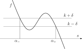
Figure 2: A typical image of $\alpha_{-},\alpha_{+}$

Proof.

Let $Z_{1},Z_{2}\in C^{1}([0,\infty))$ be the unique solutions of the problems

$$\ \left\{\begin{array}[]{ll}\dot{Z_{1}}=f(Z_{1})-k-\delta,\quad t>0,\vspace{6pt}\\ Z_{1}(0)=s_{1},\end{array}\right.\quad\mbox{and}\quad\ \left\{\begin{array}[]{ll}\dot{Z_{2}}=f(Z_{2})-k+\delta,\quad t>0,\vspace{6pt}\\ Z_{2}(0)=s_{2}.\end{array}\right.$$

It is easy to see that $\lim_{t\to\infty}Z_{1}(t)\geq\alpha_{-}$ and that $\lim_{t\to\infty}Z_{2}(t)\leq\alpha_{+}$. Thus there exists $T_{0}>0$ such that

$$Z_{1}(T_{0})\geq\alpha_{-}-\varepsilon,\quad Z_{2}(T_{0})\leq\alpha_{+}+\varepsilon.$$ (30)

Now assume that (29) holds for the above $T_{0}$ and some $\tau\geq 0$. Set

$$\widetilde{Z}_{1}(t):=Z_{1}(t-\tau),\quad\widetilde{Z}_{2}(t):=Z_{2}(t-\tau)\mbox{~{}~{}for~{}~{}}t\geq\tau.$$

Then, by Corollary 2.6, we have

$$\widetilde{Z}_{1}(\tau)=s_{1}\leq Y(\tau;s)\leq s_{2}=\widetilde{Z}_{2}(\tau)\mbox{~{}~{}for all~{}~{}}s\in[s_{1},s_{2}].$$

Let $\mathcal{L}$ be as defined in (28). It follows from (29) that

$$\mathcal{L}(\widetilde{Z}_{1}(t))\leq\mathcal{L}(Y(t;s))=0\leq\mathcal{L}(\widetilde{Z}_{2}(t))\mbox{~{}~{}for all~{}~{}}t\in[\tau,\tau+T_{0}],s\in[s_{1},s_{2}].$$

Hence, by Proposition 5.1, we have

$$\widetilde{Z}_{1}(t)\leq Y(t;s)\leq\widetilde{Z}_{2}(t)\mbox{~{}~{}for all~{}~{}}t\in[\tau,\tau+T_{0}],s\in[s_{1},s_{2}].$$

Setting $t=\tau+T_{0}$ and recalling (30), we obtain

$$\alpha_{-}-\varepsilon\leq Y(\tau+T_{0};s)\leq\alpha_{+}+\varepsilon\mbox{~{}~{}for all~{}~{}}s\in[s_{1},s_{2}].$$

The lemma is proved. ∎

Lemma 5.3.

Let $u$ be the solution of Problem $(P^{\prime})$ with $u_{0}\in L^{\infty}(\Omega)$. Assume furthermore that $\langle u_{0}\rangle\not\in[s_{*},s^{*}]$. Then

1. $\omega(u_{0})=\{\langle u_{0}\rangle\}$,

2. if $\langle u_{0}\rangle<s_{*}$ (resp. $\langle u_{0}\rangle>s^{*}$), then there exists $t_{1}\geq 0$ such that for all $t\geq t_{1}$,

   $$u(x,t)\leq s_{*}\mbox{~{}~{}(resp.~{}~{}}\geq s^{*})\mbox{~{}~{}for a.e.~{}~{}}x\in\Omega.$$

Proof.

(i) We first prove that

$$\langle f(\varphi)\rangle\not\in[f(m),f(M)]\mbox{~{}~{}for all~{}~{}}\varphi\in\omega(u_{0}).$$ (31)

Suppose, to the contrary, that there exists $\varphi\in\omega(u_{0})$ such that $\langle f(\varphi)\rangle\in[f(m),f(M)].$ Then, in view of Corollary 4.4 (ii), (iii) and (iv), we have

$$s_{*}\leq\varphi(x)\leq s^{*}\mbox{~{}~{}for a.e.~{}~{}}x\in\Omega.$$

This together with the mass conservation yields

$$\langle u_{0}\rangle=\langle\varphi\rangle\in[s_{*},s^{*}],$$

which contradicts the hypothesis of the lemma. Thus (31) holds. Consequently, by Corollary 4.4 (i), any element $\varphi\in\omega(u_{0})$ satisfies

$$\varphi(x)=\langle u_{0}\rangle\mbox{~{}~{}for a.e.~{}~{}}x\in\Omega.$$

Therefore, $\omega(u_{0})$ has the unique element $\langle u_{0}\rangle$.

(ii) We only consider the case where $\langle u_{0}\rangle<s_{*}$. The proof of the other case is similar and we omit it. Set

$$m_{0}:=\langle u_{0}\rangle<s_{*}.$$

Choose $\delta>0$ such that $f(m_{0})-\delta>f(s_{*})$. Then the equation $f(s)=f(m_{0})+\delta$ (resp. $f(s)=f(m_{0})-\delta$) has a unique root, which we denote by $\alpha_{-}$ (resp. $\alpha_{+}$). Clearly we have

$$\alpha_{-}<m_{0}<\alpha_{+}<s_{*}.$$

Choose $\varepsilon>0$ such that

$$\alpha_{-}-\varepsilon<\alpha_{+}+\varepsilon<s_{*}.$$

It follows from (i) that $u(t)\to m_{0}$ in $L^{1}(\Omega)$ as $t\to\infty$. Hence $\lambda(t)\to f(m_{0})$ as $t\to\infty$. Consequently, there exits $\tau\geq 0$ such that

$$|\lambda(t)-m_{0}|\leq\delta\mbox{~{}~{}for all~{}~{}}t\geq\tau.$$ (32)

Let $s_{1},s_{2}$ be as in $\bf(H)$. Then it follows from (32) and Lemma 5.2 that there exists $T_{0}>0$ such that

$$\alpha_{-}-\varepsilon\leq Y(\tau+T_{0},s)\leq\alpha_{+}+\varepsilon\mbox{~{}~{}for all~{}~{}}s\in[s_{1},s_{2}].$$

This, together with (12), implies

$$\alpha_{-}-\varepsilon\leq u(x,\tau+T_{0})\leq\alpha_{+}+\varepsilon\mbox{~{}~{}for a.e.~{}~{}}x\in\Omega.$$

In particularly, $u(x,\tau+T_{0})\leq s_{*}\mbox{~{}~{}for a.e.~{}~{}}x\in\Omega.$ Hence, by Corollary 2.7 (ii), we have for all $t\geq\tau+T_{0}$,

$$u(x,t)\leq s_{*}\mbox{~{}~{}for a.e.~{}~{}}x\in\Omega.$$

This completes the proof of Lemma 5.3. ∎

Proof of Theorem 1.5.

It follows from Lemma 5.3 (i) that $\omega(u_{0})=\{\langle u_{0}\rangle\}.$ Hence $u(t)\to\langle u_{0}\rangle$ in $L^{1}(\Omega)$ as $t\to\infty$. We will show that the convergence takes place in $L^{\infty}(\Omega)$ and that the estimate (8) holds. We will only consider the case $\langle u_{0}\rangle<s_{*}$, since the case $\langle u_{0}\rangle>s^{*}$ can be treated similarly. Then, in view of Lemma 5.3 (ii), we may assume without loss of generality that

$$u(x,t)\leq s_{*}\ \ \mbox{for \ a.e.}\ x\in\Omega,\ t\geq 0.$$ (33)

Thus we may choose $s_{1},s_{2}$ such that

$$s_{1}<\langle u_{0}\rangle<s_{2}\leq s_{*}.$$

Since $u(t)\to\langle u_{0}\rangle$ in $L^{1}(\Omega)$ as $t\to\infty$, we have $\lambda(t):=\langle f(u(t))\rangle\to f(\langle u_{0}\rangle)$ as $t\to\infty$. Hence

$$f(s_{1})\geq\lambda(t)\geq f(s_{2})$$ (34)

for all large $t\geq 0$. Without loss of generality we may assume that (34) holds for all $t\geq 0$. Now we set $v_{1}(t):=Y(t;s_{1}),\,v_{2}(t):=Y(t;s_{2})$. Then

$$\dot{v}_{1}=f(v_{1})-\lambda(t),\ \ v_{1}(0)=s_{1},\quad\ \ \dot{v}_{2}=f(v_{2})-\lambda(t),\ \ v_{2}(0)=s_{2}.$$

Therefore, by (34),

$${\mathcal{L}}(s_{1})\leq 0={\mathcal{L}}(v_{1})={\mathcal{L}}(v_{2})\leq{\mathcal{L}}(s_{2}).$$

Hence, by Proposition 5.1 and the monotonicity of $Y(t;s)$ in $s$, we have

$$s_{1}\leq v_{1}(t)\leq u(x,t)\leq v_{2}(t)\leq s_{2}\quad\ \hbox{for \ \ a.e.}\ x\in\Omega,\ t\geq 0.$$ (35)

Define $\rho(t):=v_{2}(t)-v_{1}(t)$. Then

$$\dot{\rho}=f(v_{2})-f(v_{1})=f^{\prime}(\xi(t))\rho,$$

where $\xi(t)\in[v_{1}(t),v_{2}(t)]\subset[s_{1},s_{2}]$. Hence, by (35),

$$\dot{\rho}(t)\leq-\mu\rho(t),\quad\hbox{where}\ \ \ -\mu:=\max_{s\in[s_{1},s_{2}]}f^{\prime}(s)<0.$$

Consequently

$$v_{2}(t)-v_{1}(t):=\rho(t)=O(e^{-\mu t}).$$

Combining this and (35), we obtain

$$\|u(t)-\langle u_{0}\rangle\|_{L^{\infty}(\Omega)}=O(e^{-\mu t}).$$

This completes the proof of Theorem 1.5. ∎

6 Proof of Theorem 1.6

In this section we discuss the large time behavior of the solution under the assumption $s_{*}\leq\langle u_{0}\rangle\leq s^{*}$ and prove Theorem 1.6. The proof is divided into two steps. Subsection 6.1 deals with the special case where $s_{*}\leq u_{0}(x)\leq s^{*}$ a.e. $x\in\Omega$, and Subsection 6.2 deals with the general case.

6.1 The case $s_{*}\leq u_{0}\leq s^{*}$ a.e. in $\Omega$

The main result of this subsection is Theorem 6.5 below. First note that for each $u_{0}\in L^{\infty}(\Omega)$ with $s_{*}\leq u_{0}\leq s^{*}$ a.e. in $\Omega$ there exist subsets $\widetilde{\Omega},\mathcal{N}\subset\Omega$ such that

$$|\mathcal{N}|=0,\quad\widetilde{\Omega}\cup\mathcal{N}=\Omega,$$

$$s_{*}\leq u_{0}(x)\leq s^{*}\mbox{~{}~{}for all~{}~{}}x\in\widetilde{\Omega}.$$

We define for each $t\geq 0$,

$$\Omega_{-}(t):=\{x\in\widetilde{\Omega}:Y(t;u_{0}(x))\leq m\},$$

$$\Omega_{0}(t):=\{x\in\widetilde{\Omega}:m<Y(t;u_{0}(x))<M\},$$

$$\Omega_{+}(t):=\{x\in\widetilde{\Omega}:Y(t;u_{0}(x))\geq M\}.$$

Lemma 6.1.

Suppose that

$$s_{*}\leq u_{0}\leq s^{*}\mbox{~{}~{}a.e. in~{}~{}}\Omega.$$

Then for every $t^{\prime}>t\geq 0$, $s\in[s_{*},s^{*}]$,

1. if $Y(t;s)\leq m$, then $Y(t^{\prime};s)\leq m$ for every $t^{\prime}>t\geq 0$;

2. if $Y(t;s)\geq M$, then $Y(t^{\prime};s)\geq M$ for every $t^{\prime}>t\geq 0$.

As a consequence, for every $t^{\prime}>t\geq 0$,

$$\Omega_{-}(t)\subset\Omega_{-}(t^{\prime}),~{}~{}~{}~{}\Omega_{+}(t)\subset\Omega_{+}(t^{\prime})\mbox{~{}~{}~{}~{}and~{}~{}~{}~{}}\Omega_{0}(t)\supset\Omega_{0}(t^{\prime}).$$

In other words, $\Omega_{-}(t),\Omega_{+}(t)$ are monotonically expanding in $t$ while $\Omega_{0}(t)$ is monotonically shrinking in $t$.

Proof.

It follows from Corollary 2.7 (i) that for all $t\geq 0$,

$$s_{*}\leq u(x,t)\leq s^{*}\mbox{~{}~{}for a.e.~{}~{}}x\in\Omega,$$

so that

$$f(m)\leq\langle f(u(t))\rangle=\lambda(t)\leq f(M).$$

Consequently

$$\mathcal{L}(m)\geq 0\mbox{~{}~{}and~{}~{}}\mathcal{L}(M)\leq 0,$$

where $\mathcal{L}$ is as defined in (28). Hence (i), (ii) follow from Proposision 5.1. ∎

We define

$$\Omega_{-}(\infty):=\bigcup_{t\geq 0}\Omega_{-}(t),\quad\Omega_{0}(\infty):=\bigcap_{t\geq 0}\Omega_{0}(t),\quad\Omega_{+}(\infty):=\bigcup_{t\geq 0}\Omega_{+}(t).$$ (36)

The following result is an immediate consequence of Lemma 6.1.

Corollary 6.2.

Suppose that $s_{*}\leq u_{0}\leq s^{*}\mbox{~{}~{}a.e. in~{}~{}}\Omega$. Then $\Omega_{-}(\infty),\Omega_{0}(\infty),\Omega_{+}(\infty)$ are pairwise disjoint and

$$\Omega=\Omega_{-}(\infty)\cup\Omega_{0}(\infty)\cup\Omega_{+}(\infty)\cup\mathcal{N}.$$

Moreover,

$$\Omega_{-}(\infty) =\{x\in\widetilde{\Omega}:\exists t_{0}\geq 0\mbox{~{}~{}such that~{}~{}}Y(t;u_{0}(x))\leq m\mbox{~{}~{}for all~{}~{}}t\geq t_{0}\},$$

$$\Omega_{0}(\infty) =\{x\in\widetilde{\Omega}:m<Y(t;u_{0}(x))<M\mbox{~{}~{}for all~{}~{}}t\geq 0\},$$

$$\Omega_{+}(\infty) =\{x\in\widetilde{\Omega}:\exists t_{0}\geq 0\mbox{~{}~{}such that~{}~{}}Y(t;u_{0}(x))\geq M\mbox{~{}~{}for all~{}~{}}t\geq t_{0}\}.$$

Proposition 6.3.

Assume that

$$s_{*}\leq u_{0}\leq s^{*}\mbox{~{}~{}a.e. in~{}~{}}\Omega.$$ (37)

Then

$$\langle f(\varphi)\rangle\in[f(m),f(M)]\mbox{~{}~{}for all~{}~{}}\varphi\in\omega(u_{0}).$$ (38)

Furthermore,

1. If $f(m)<\langle f(\varphi)\rangle<f(M)$, then

   $$\varphi=a_{-}\chi_{\Omega_{-}(\infty)}+a_{0}\chi_{\Omega_{0}(\infty)}+a_{+}\chi_{\Omega_{+}(\infty)},$$

   where $s_{*}<a_{-}<a_{0}<a_{+}<s^{*}$ are the roots of the equation $f(s)=\langle f(\varphi)\rangle$.

2. If $\langle f(\varphi)\rangle=f(m)$, then

   $$\varphi=m\chi_{\Omega_{-}(\infty)}+s^{*}\chi_{\Omega_{0}(\infty)\cup\Omega_{+}(\infty)}.$$

3. If $\langle f(\varphi)\rangle=f(M)$, then

   $$\varphi=s_{*}\chi_{\Omega_{-}(\infty)\cup\Omega_{0}(\infty)}+M\chi_{\Omega_{+}(\infty)}.$$

Proof.

First we prove (38). Indeed, if there exists $\psi\in\omega(u_{0})$ such that $\langle f(\psi)\rangle\not\in[f(m),f(M)]$, then it follows from Corollary 4.4 (i) that

$$\psi\equiv\langle u_{0}\rangle\not\in[s_{*},s^{*}],$$

which is in contradiction with (37). Thus (38) holds. Next we remark that there exists a sequence $t_{n}\to\infty$ such that

$$Y(t_{n};u_{0}(x))\to\varphi(x)\quad\mbox{for a.e.~{}}x\in\Omega\mbox{~{}~{}as~{}~{}}n\to\infty.$$

This, together with Corollary 6.2, implies that

$$\varphi(x)\leq m\quad\quad\quad\mbox{~{}~{}for a.e.~{}~{}}x\in\Omega_{-}(\infty),$$

$$m\leq\varphi(x)\leq M\mbox{~{}~{}~{}~{}for a.e.~{}~{}}x\in\Omega_{0}(\infty),$$

$$\varphi(x)\geq M\quad\quad\quad\mbox{~{}~{}for a.e.~{}~{}}x\in\Omega_{+}(\infty).$$

Thus we deduce from Corollary 4.4 that

$$\varphi=a_{-}\mbox{~{}~{}a.e. in~{}~{}}\Omega_{-}(\infty),\quad\varphi=a_{0}\mbox{~{}~{}a.e. in~{}~{}}\Omega_{0}(\infty),$$

$$\varphi=a_{+}\mbox{~{}~{}a.e. in~{}~{}}\Omega_{+}(\infty),$$

if $\langle f(\varphi)\rangle\in(f(m),f(M))$. This proves (i). The assertions (ii), (iii) also follow from Corollary 4.4. The proposition is proved. ∎

Lemma 6.4.

Assume that $s,\widetilde{s}$ satisfy

$$m<Y(t;s)<M,\quad m<Y(t;\widetilde{s})<M\mbox{~{}~{}for all~{}~{}}t\geq 0.$$

Assume further that there exists a sequence $t_{n}\to\infty$ satisfying

$$Y(t_{n};s)\to a,\quad Y(t_{n};\widetilde{s})\to a\mbox{~{}~{}as~{}~{}}n\to\infty,$$ (39)

for some $a\in[m,M]$. Then $s=\widetilde{s}.$

Proof.

Assume that $s\leq\widetilde{s}$. Then

$$m<Y(t;s)\leq Y(t;\widetilde{s})<M\mbox{~{}~{}for all~{}~{}}t\geq 0.$$

Since $f$ is increasing on $[m,M]$, we have

$$f(Y(t;s))\leq f(Y(t;\widetilde{s}))\mbox{~{}~{}for all~{}~{}}t\geq 0.$$

Consequently, the function $h(t):=Y(t;\widetilde{s})-Y(t;s)$ satisfies

$$h^{\prime}(t)=\dot{Y}(t;\widetilde{s})-\dot{Y}(t;s)=f(Y(t,\widetilde{s}))-f(Y(t,s))\geq 0.$$

Therefore $h(t)\geq h(0)=\widetilde{s}-s$. On the other hand, (39) yields $\lim_{n\to\infty}h(t_{n})=0$. Hence $s=\widetilde{s}$. ∎

Theorem 6.5.

Assume that $s_{*}\leq u_{0}\leq s^{*}$ a.e. in $\Omega$. Suppose further that

$$|\{x:u_{0}(x)=s\}|=0\mbox{~{}~{}for all~{}~{}}s\in(m,M).$$

Then $\omega(u_{0})$ contains only one element $\varphi$, and it is a step function. Moreover, $\varphi$ is given by

$$\varphi=a_{-}\chi_{\Omega_{-}(\infty)}+a_{+}\chi_{\Omega_{+}(\infty)},$$ (40)

where $\Omega_{-}(\infty),\Omega_{+}(\infty)$ are defined by (36) and $a_{+},a_{-}$ are constants satisfying

$$s_{*}\leq a_{-}\leq m,\quad M\leq a_{+}\leq s^{*},\quad f(a_{-})=f(a_{+})=\langle f(\varphi)\rangle.$$

Proof.

We first show that

$$|\Omega_{0}(\infty)|=0.$$

Suppose, by contradiction, that

$$|\Omega_{0}(\infty)|>0$$

and let $\varphi\in\omega(u_{0})$. Then in view of Proposition 6.3, $\varphi$ is constant on $\Omega_{0}(\infty)$, say, $\varphi=a\in[m,M]$ a.e. on $\Omega_{0}(\infty)$. Let $t_{n}\to\infty$ be such that

$$u(t_{n})\to\varphi\mbox{~{}~{}in~{}~{}}L^{1}(\Omega)\mbox{~{}~{}as~{}~{}}n\to\infty,$$

or equivalently,

$$Y(t_{n};u_{0}(\cdot))\to\varphi\mbox{~{}~{}in~{}~{}}L^{1}(\Omega)\mbox{~{}~{}as~{}~{}}n\to\infty.$$

Then there exists a subsequence $\{t_{n_{k}}\}$ such that

$$Y(t_{n_{k}};u_{0}(x))\to a\mbox{~{}~{}as~{}~{}}k\to\infty\mbox{~{}~{}a.e.~{}~{}}x\in\Omega_{0}(\infty).$$

We deduce from Lemma 6.4 that there exists $\alpha\in(m,M)$ such that

$$u_{0}=\alpha\mbox{~{}~{}on~{}~{}}\Omega_{0}(\infty),$$

which implies by the hypothesis in Theorem 6.5 that

$$|\Omega_{0}(\infty)|=0.$$

This and Proposition 6.3 imply that any element $\varphi\in\omega(u_{0})$ has the form (40).

Next we prove that $\omega(u_{0})$ contains only one element. We argue by contradiction, suppose that there exist $\varphi,\overline{\varphi}\in\omega(u_{0})$ with $\varphi\neq\overline{\varphi}$. By what we have shown above, we can write:

$$\varphi=a_{-}\chi_{\Omega_{-}(\infty)}+a_{+}\chi_{\Omega_{+}(\infty)},\quad\overline{\varphi}=\overline{a}_{-}\chi_{\Omega_{-}(\infty)}+\overline{a}_{+}\chi_{\Omega_{+}(\infty)},$$

where the constants $a_{\pm},\overline{a}_{\pm}$ satisfy

$$a_{-},\overline{a}_{-}\in[s_{*},m],\quad a_{+},\overline{a}_{+}\in[M,s^{*}],$$

$$f(a_{-})=f(a_{+})=\langle f(\varphi)\rangle,\quad f(\overline{a}_{-})=f(\overline{a}_{+})=\langle f(\overline{\varphi})\rangle.$$

Since $\varphi\neq\overline{\varphi}$, we have $(a_{-},a_{+})\neq(\overline{a}_{-},\overline{a}_{+})$, which implies $\langle f(\varphi)\rangle\neq\langle f(\overline{\varphi})\rangle$. Without loss of generality, we may assume that

$$f(m)\leq\langle f(\varphi)\rangle<\langle f(\overline{\varphi})\rangle\leq f(M).$$

Since $f$ is strictly decreasing on $(-\infty,m]$ and $[M,\infty)$, we see that $a_{-}>\overline{a}_{-},a_{+}>\overline{a}_{+}$. Then, using the mass conservation property, we obtain

$$\int_{\Omega}u_{0}=a_{-}|\Omega_{-}(\infty)|+a_{+}|\Omega_{+}(\infty)|>\overline{a}_{-}|\Omega_{-}(\infty)|+\overline{a}_{+}|\Omega_{+}(\infty)|=\int_{\Omega}u_{0},$$

which gives a contradiction. Hence $\omega(u_{0})$ contains only one element. This completes the proof of Theorem 6.5. ∎

6.2 The general case

In this subsection, we prove Theorem 1.6 for the general case. We begin with the following lemma whose proof is similar to that of Lemma 5.3 (ii).

Lemma 6.6.

Let $u$ be the solution of Problem $(P^{\prime})$ with $u_{0}\in L^{\infty}(\Omega)$. If there exists $\varphi\in\omega(u_{0})$ such that

$$\langle f(\varphi)\rangle\in(f(m),f(M)),$$

then there exists $t_{1}\geq 0$ such that for all $t\geq t_{1}$,

$$s_{*}\leq u(x,t)\leq s^{*}\mbox{~{}~{}for a.e.~{}~{}}x\in\Omega.$$

Proof.

Since $\langle f(\varphi)\rangle\in(f(m),f(M))$, the equations $f(s)=\langle f(\varphi)\rangle$ has the three roots $a_{-}<a_{0}<a_{+}$. Moreover, we have

$$s_{*}<a_{-},\quad a_{+}<s^{*}.$$

Choose $\delta>0$ such that $f(m)<\langle f(\varphi)\rangle-\delta<\langle f(\varphi)\rangle+\delta<f(M)$ and set

$$\alpha_{-}:=\min\{s\in{\mathbb{R}}:f(s)=k+\delta\},\quad\alpha_{+}:=\max\{s\in{\mathbb{R}}:f(s)=k-\delta\}.$$

Clearly, we have

$$s_{*}<\alpha_{-}<\alpha_{+}<s^{*}.$$

Choose $\varepsilon>0$ such that

$$s_{*}<\alpha_{-}-\varepsilon<\alpha_{+}+\varepsilon<s^{*}$$ (41)

and let $s_{1},s_{2}$ be as in $\bf(H)$. Let $T_{0}$ be as in Lemma 5.2. It follows from Corollary 4.3 that there exits $\tau>0$ such that

$$|\lambda(t)-\langle f(\varphi)\rangle|\leq\delta\mbox{~{}~{}for all~{}~{}}t\in[\tau,\tau+T_{0}].$$

Thus, Lemma 5.2 yields

$$\alpha_{-}-\varepsilon\leq Y(\tau+T_{0};s)\leq\alpha_{+}+\varepsilon\mbox{~{}~{}for all~{}~{}}s\in[s_{1},s_{2}].$$

This, together with (41) and (12), implies

$$s_{*}\leq u(x,\tau+T_{0})\leq s^{*}\mbox{~{}~{}for a.e.~{}~{}}x\in\Omega.$$

Hence the assertion of Lemma 6.6 follows from Corollary 2.7 (i). ∎

Proof of Theorem 1.6.

First we prove that

$$\langle f(\varphi)\rangle\in[f(m),f(M)]\mbox{~{}~{}for all~{}~{}}\varphi\in\omega(u_{0}).$$ (42)

Indeed, if there exists $\psi\in\omega(u_{0})$ such that $\langle f(\psi)\rangle\not\in[f(m),f(M)]$, then it follows from Corollary 4.4 (i) that $\psi\equiv\langle u_{0}\rangle\not\in[s_{*},s^{*}],$ which contradicts the assumption of the theorem. Since $\omega(u_{0})$ is connected in $L^{1}(\Omega)$, the set $\{\langle f(\varphi)\rangle:\varphi\in\omega(u_{0})\}$ is connected in ${\mathbb{R}}$. This, together with (42), implies that we have one and only one of the following cases:

1. either there exists $\varphi\in\omega(u_{0})$ such that $\langle f(\varphi)\rangle\in(f(m),f(M))$,

2. or we have $\langle f(\varphi)\rangle=f(m)\mbox{~{}~{}for all~{}~{}}\varphi\in\omega(u_{0}),$

3. or we have $\langle f(\varphi)\rangle=f(M)\mbox{~{}~{}for all~{}~{}}\varphi\in\omega(u_{0}).$

If (i) holds, then by Lemma 6.6, there exists $t_{1}\geq 0$ such that

$$s_{*}\leq u(x,t_{1})\leq s^{*}\mbox{~{}~{}for a.e~{}~{}}x\in\Omega.$$

It is also clear from (9) and the strict monotonicity of $s\mapsto Y(t;s)$ that $u(x,t_{1}):=Y(t_{1};u_{0}(x))$ satisfies

$$|\{x:u(x,t_{1})=s\}|=0\mbox{~{}~{}for all~{}~{}}s\in{\mathbb{R}}.$$

Hence the assertion of Theorem 1.6 follows from Theorem 6.5 by regarding $u(x,t_{1})$ as the initial data.

If (ii) holds, then it follows from Corollary 4.4 (iii) that for each $\varphi\in\omega(u_{0})$, $\varphi$ is written — up to modification on a set of zero measure — in the form

$$\varphi(x)=m\chi_{A_{-}}(x)+s^{*}\chi_{A_{+}}(x)$$ (43)

for some disjoint subsets $A_{-},A_{+}$ satisfying $A_{-}\cup A_{+}=\Omega.$ Now let

$${\Omega_{+}}(t)=\{x\in\Omega:Y(t;u_{0}(x))\geq M\}.$$

Then, since $\lambda(t):=\langle f(u(t))\rangle\to f(m)$ as $t\to\infty,$ there exists $T>0$ such that

$$\mathcal{L}(M)=-f(M)+\lambda(t)\leq 0\quad\ \hbox{for all}\ \ t\geq T,$$

where $\mathcal{L}$ is as defined in (28). Therefore, if $Y(t_{1};u_{0}(x))\geq M$ for some $t_{1}\in[T,\infty)$, then $Y(t;u_{0}(x))\geq M$ for all $t\geq t_{1}$. This implies that $\Omega_{+}(t)$ is monotonically expanding for all $t\geq T$. Hence the limit $\Omega_{+}(\infty)$ exists and we have

$$\Omega_{+}(\infty)=\{x\in\Omega:\exists t_{0}\geq 0\mbox{~{}~{}such that~{}~{}}Y(t;u_{0}(x))\geq M\mbox{~{}~{}for all~{}~{}}t\geq t_{0}\}.$$

It is also easily seen that the set $A_{+}$ in (43) coincides with this limit, hence

$$A_{-}=\Omega\setminus\Omega_{+}(\infty),\ A_{+}=\Omega_{+}(\infty).$$

Since any element of $\omega(u_{0})$ is written in this form, $\omega(u_{0})$ contains only one element, which establishes the assertion of theorem.

The case (iii) can be treated by the same argument as (ii). This completes the proof of Theorem 1.6. ∎

References

- [1] M. Alfaro, D. Hilhorst, H. Matano, The singular limit of the Allen-Cahn equation and the FitzHugh-Nagumo system, J. Differential Equations 245 (2008), 505–565.
- [2] L. Ambrosio, N. Fusco, D. Pallara, Functions of bounded variation and free discontinuity problems, Oxford University Press, 2000.
- [3] S. Boussaïd, D. Hilhorst, T. N. Nguyen, Convergence to steady state for the solutions of a nonlocal reaction-diffusion equation, to appear in Evolution Equations and Control Theory.
- [4] X. Chen, Generation and propagation of interfaces for reaction-diffusion equations, J. Differential Equations 96 (1992), 116–141.
- [5] P. de Mottoni, M. Schatzman, Geometrical evolution of developed interfaces, Trans. Amer. Math. Soc. 347 (1995), 1533–1589.
- [6] L. Evans, R. F. Gariepy, Measure theory and fine properties of functions, CRC Press, 1992.
- [7] J. K. Hale, Ordinary differential equations, Wiley, New York, .
- [8] D. Hilhorst, H. Matano, T.N. Nguyen, H. Weber, Generation of interface for the mass conserved Allen-Cahn equation, in preparation.
- [9] S. Kesavan, Symmetrization Applications, World Scientific Publishing, 2006.
- [10] H. Matano, Nonincrease of the lap-number of a solution for a one-dimensional semilinear parabolic equation, J. Fac. Sci. Univ. Tokyo Sect. IA Math. 29 (1982), 401–441.
- [11] J. C. Robinson, Infinite-dimensional dynamical systems, Cambridge University Press, .
- [12] J. Rubinstein, P. Sternberg, Nonlocal reaction-diffusion equations and nucleation, IMA Journal of Applied Mathematics 48 (1992), 249–264.