The 2012 flare of PG 1553+113 seen with H.E.S.S. and Fermi-LAT: Constraints on the source redshift
and Lorentz invariance violation
H.E.S.S. Collaboration,
A. Abramowski 11affiliation: Universität Hamburg, Institut für Experimentalphysik, Luruper Chaussee 149, D 22761 Hamburg, Germany ,
F. Aharonian 22affiliation: Max-Planck-Institut für Kernphysik, P.O. Box 103980, D 69029 Heidelberg, Germany 33affiliation: Dublin Institute for Advanced Studies, 31 Fitzwilliam Place, Dublin 2, Ireland 44affiliation: National Academy of Sciences of the Republic of Armenia, Marshall Baghramian Avenue, 24, 0019 Yerevan, Republic of Armenia ,
F. Ait Benkhali 22affiliation: Max-Planck-Institut für Kernphysik, P.O. Box 103980, D 69029 Heidelberg, Germany ,
A.G. Akhperjanian 55affiliation: Yerevan Physics Institute, 2 Alikhanian Brothers St., 375036 Yerevan, Armenia 44affiliation: National Academy of Sciences of the Republic of Armenia, Marshall Baghramian Avenue, 24, 0019 Yerevan, Republic of Armenia ,
E.O. Angüner 66affiliation: Institut für Physik, Humboldt-Universität zu Berlin, Newtonstr. 15, D 12489 Berlin, Germany ,
M. Backes 77affiliation: University of Namibia, Department of Physics, Private Bag 13301, Windhoek, Namibia ,
S. Balenderan 88affiliation: University of Durham, Department of Physics, South Road, Durham DH1 3LE, U.K. ,
A. Balzer 99affiliation: GRAPPA, Anton Pannekoek Institute for Astronomy, University of Amsterdam, Science Park 904, 1098 XH Amsterdam, The Netherlands ,
A. Barnacka 1010affiliation: Obserwatorium Astronomiczne, Uniwersytet Jagielloński, ul. Orla 171, 30-244 Kraków, Poland 1111affiliation: now at Harvard-Smithsonian Center for Astrophysics, 60 Garden St, MS-20, Cambridge, MA 02138, USA ,
Y. Becherini 1212affiliation: Department of Physics and Electrical Engineering, Linnaeus University, 351 95 Växjö, Sweden ,
J. Becker Tjus 1313affiliation: Institut für Theoretische Physik, Lehrstuhl IV: Weltraum und Astrophysik, Ruhr-Universität Bochum, D 44780 Bochum, Germany ,
D. Berge 1414affiliation: GRAPPA, Anton Pannekoek Institute for Astronomy and Institute of High-Energy Physics, University of Amsterdam, Science Park 904, 1098 XH Amsterdam, The Netherlands ,
S. Bernhard 1515affiliation: Institut für Astro- und Teilchenphysik, Leopold-Franzens-Universität Innsbruck, A-6020 Innsbruck, Austria ,
K. Bernlöhr 22affiliation: Max-Planck-Institut für Kernphysik, P.O. Box 103980, D 69029 Heidelberg, Germany 66affiliation: Institut für Physik, Humboldt-Universität zu Berlin, Newtonstr. 15, D 12489 Berlin, Germany ,
E. Birsin 66affiliation: Institut für Physik, Humboldt-Universität zu Berlin, Newtonstr. 15, D 12489 Berlin, Germany ,
J. Biteau 1616affiliation: Laboratoire Leprince-Ringuet, Ecole Polytechnique, CNRS/IN2P3, F-91128 Palaiseau, France 1717affiliation: now at Santa Cruz Institute for Particle Physics, Department of Physics, University of California at Santa Cruz, Santa Cruz, CA 95064, USA ,
M. Böttcher 1818affiliation: Centre for Space Research, North-West University, Potchefstroom 2520, South Africa ,
C. Boisson 1919affiliation: LUTH, Observatoire de Paris, CNRS, Université Paris Diderot, 5 Place Jules Janssen, 92190 Meudon, France ,
J. Bolmont 2020affiliation: LPNHE, Université Pierre et Marie Curie Paris 6, Université Denis Diderot Paris 7, CNRS/IN2P3, 4 Place Jussieu, F-75252, Paris Cedex 5, France ,
P. Bordas 2121affiliation: Institut für Astronomie und Astrophysik, Universität Tübingen, Sand 1, D 72076 Tübingen, Germany ,
J. Bregeon 2222affiliation: Laboratoire Univers et Particules de Montpellier, Université Montpellier 2, CNRS/IN2P3, CC 72, Place Eugène Bataillon, F-34095 Montpellier Cedex 5, France ,
F. Brun 2323affiliation: DSM/Irfu, CEA Saclay, F-91191 Gif-Sur-Yvette Cedex, France **affiliation: Corresponding authors:
D.A. Sanchez, david.sanchez@lapp.in2p3.fr, F. Brun, francois.brun@cea.fr, C. Couturier, camille.couturier@lpnhe.in2p3.fr, J. Lefaucheur, julien.lefaucheur@apc.univ-paris7.fr, J.-P. Lenain, jlenain@lpnhe.in2p3.fr ,
P. Brun 2323affiliation: DSM/Irfu, CEA Saclay, F-91191 Gif-Sur-Yvette Cedex, France ,
M. Bryan 99affiliation: GRAPPA, Anton Pannekoek Institute for Astronomy, University of Amsterdam, Science Park 904, 1098 XH Amsterdam, The Netherlands ,
T. Bulik 2424affiliation: Astronomical Observatory, The University of Warsaw, Al. Ujazdowskie 4, 00-478 Warsaw, Poland ,
S. Carrigan 22affiliation: Max-Planck-Institut für Kernphysik, P.O. Box 103980, D 69029 Heidelberg, Germany ,
S. Casanova 2525affiliation: Instytut Fizyki Ja̧drowej PAN, ul. Radzikowskiego 152, 31-342 Kraków, Poland 22affiliation: Max-Planck-Institut für Kernphysik, P.O. Box 103980, D 69029 Heidelberg, Germany ,
P.M. Chadwick 88affiliation: University of Durham, Department of Physics, South Road, Durham DH1 3LE, U.K. ,
N. Chakraborty 22affiliation: Max-Planck-Institut für Kernphysik, P.O. Box 103980, D 69029 Heidelberg, Germany ,
R. Chalme-Calvet 2020affiliation: LPNHE, Université Pierre et Marie Curie Paris 6, Université Denis Diderot Paris 7, CNRS/IN2P3, 4 Place Jussieu, F-75252, Paris Cedex 5, France ,
R.C.G. Chaves 2222affiliation: Laboratoire Univers et Particules de Montpellier, Université Montpellier 2, CNRS/IN2P3, CC 72, Place Eugène Bataillon, F-34095 Montpellier Cedex 5, France ,
M. Chrétien 2020affiliation: LPNHE, Université Pierre et Marie Curie Paris 6, Université Denis Diderot Paris 7, CNRS/IN2P3, 4 Place Jussieu, F-75252, Paris Cedex 5, France ,
S. Colafrancesco 2626affiliation: School of Physics, University of the Witwatersrand, 1 Jan Smuts Avenue, Braamfontein, Johannesburg, 2050 South Africa ,
G. Cologna 2727affiliation: Landessternwarte, Universität Heidelberg, Königstuhl, D 69117 Heidelberg, Germany ,
J. Conrad 2828affiliation: Oskar Klein Centre, Department of Physics, Stockholm University, Albanova University Center, SE-10691 Stockholm, Sweden 2929affiliation: Wallenberg Academy Fellow, ,
C. Couturier 2020affiliation: LPNHE, Université Pierre et Marie Curie Paris 6, Université Denis Diderot Paris 7, CNRS/IN2P3, 4 Place Jussieu, F-75252, Paris Cedex 5, France **affiliation: Corresponding authors:
D.A. Sanchez, david.sanchez@lapp.in2p3.fr, F. Brun, francois.brun@cea.fr, C. Couturier, camille.couturier@lpnhe.in2p3.fr, J. Lefaucheur, julien.lefaucheur@apc.univ-paris7.fr, J.-P. Lenain, jlenain@lpnhe.in2p3.fr ,
Y. Cui 2121affiliation: Institut für Astronomie und Astrophysik, Universität Tübingen, Sand 1, D 72076 Tübingen, Germany ,
M. Dalton 3030affiliation: Université Bordeaux 1, CNRS/IN2P3, Centre d’Études Nucléaires de Bordeaux Gradignan, 33175 Gradignan, France 3131affiliation: Funded by contract ERC-StG-259391 from the European Community, ,
I.D. Davids 1818affiliation: Centre for Space Research, North-West University, Potchefstroom 2520, South Africa 77affiliation: University of Namibia, Department of Physics, Private Bag 13301, Windhoek, Namibia ,
B. Degrange 1616affiliation: Laboratoire Leprince-Ringuet, Ecole Polytechnique, CNRS/IN2P3, F-91128 Palaiseau, France ,
C. Deil 22affiliation: Max-Planck-Institut für Kernphysik, P.O. Box 103980, D 69029 Heidelberg, Germany ,
P. deWilt 3232affiliation: School of Chemistry & Physics, University of Adelaide, Adelaide 5005, Australia ,
A. Djannati-Ataï 3333affiliation: APC, AstroParticule et Cosmologie, Université Paris Diderot, CNRS/IN2P3, CEA/Irfu, Observatoire de Paris, Sorbonne Paris Cité, 10, rue Alice Domon et Léonie Duquet, 75205 Paris Cedex 13, France ,
W. Domainko 22affiliation: Max-Planck-Institut für Kernphysik, P.O. Box 103980, D 69029 Heidelberg, Germany ,
A. Donath 22affiliation: Max-Planck-Institut für Kernphysik, P.O. Box 103980, D 69029 Heidelberg, Germany ,
L.O’C. Drury 33affiliation: Dublin Institute for Advanced Studies, 31 Fitzwilliam Place, Dublin 2, Ireland ,
G. Dubus 3434affiliation: Univ. Grenoble Alpes, IPAG, F-38000 Grenoble, France
CNRS, IPAG, F-38000 Grenoble, France ,
K. Dutson 3535affiliation: Department of Physics and Astronomy, The University of Leicester, University Road, Leicester, LE1 7RH, United Kingdom ,
J. Dyks 3636affiliation: Nicolaus Copernicus Astronomical Center, ul. Bartycka 18, 00-716 Warsaw, Poland ,
M. Dyrda 2525affiliation: Instytut Fizyki Ja̧drowej PAN, ul. Radzikowskiego 152, 31-342 Kraków, Poland ,
T. Edwards 22affiliation: Max-Planck-Institut für Kernphysik, P.O. Box 103980, D 69029 Heidelberg, Germany ,
K. Egberts 3737affiliation: Institut für Physik und Astronomie, Universität Potsdam, Karl-Liebknecht-Strasse 24/25, D 14476 Potsdam, Germany ,
P. Eger 22affiliation: Max-Planck-Institut für Kernphysik, P.O. Box 103980, D 69029 Heidelberg, Germany ,
P. Espigat 3333affiliation: APC, AstroParticule et Cosmologie, Université Paris Diderot, CNRS/IN2P3, CEA/Irfu, Observatoire de Paris, Sorbonne Paris Cité, 10, rue Alice Domon et Léonie Duquet, 75205 Paris Cedex 13, France ,
C. Farnier 2828affiliation: Oskar Klein Centre, Department of Physics, Stockholm University, Albanova University Center, SE-10691 Stockholm, Sweden ,
S. Fegan 1616affiliation: Laboratoire Leprince-Ringuet, Ecole Polytechnique, CNRS/IN2P3, F-91128 Palaiseau, France ,
F. Feinstein 2222affiliation: Laboratoire Univers et Particules de Montpellier, Université Montpellier 2, CNRS/IN2P3, CC 72, Place Eugène Bataillon, F-34095 Montpellier Cedex 5, France ,
M.V. Fernandes 11affiliation: Universität Hamburg, Institut für Experimentalphysik, Luruper Chaussee 149, D 22761 Hamburg, Germany ,
D. Fernandez 2222affiliation: Laboratoire Univers et Particules de Montpellier, Université Montpellier 2, CNRS/IN2P3, CC 72, Place Eugène Bataillon, F-34095 Montpellier Cedex 5, France ,
A. Fiasson 3838affiliation: Laboratoire d’Annecy-le-Vieux de Physique des Particules, Université de Savoie, CNRS/IN2P3, F-74941 Annecy-le-Vieux, France ,
G. Fontaine 1616affiliation: Laboratoire Leprince-Ringuet, Ecole Polytechnique, CNRS/IN2P3, F-91128 Palaiseau, France ,
A. Förster 22affiliation: Max-Planck-Institut für Kernphysik, P.O. Box 103980, D 69029 Heidelberg, Germany ,
M. Füßling 3737affiliation: Institut für Physik und Astronomie, Universität Potsdam, Karl-Liebknecht-Strasse 24/25, D 14476 Potsdam, Germany ,
S. Gabici 3333affiliation: APC, AstroParticule et Cosmologie, Université Paris Diderot, CNRS/IN2P3, CEA/Irfu, Observatoire de Paris, Sorbonne Paris Cité, 10, rue Alice Domon et Léonie Duquet, 75205 Paris Cedex 13, France ,
M. Gajdus 66affiliation: Institut für Physik, Humboldt-Universität zu Berlin, Newtonstr. 15, D 12489 Berlin, Germany ,
Y.A. Gallant 2222affiliation: Laboratoire Univers et Particules de Montpellier, Université Montpellier 2, CNRS/IN2P3, CC 72, Place Eugène Bataillon, F-34095 Montpellier Cedex 5, France ,
T. Garrigoux 2020affiliation: LPNHE, Université Pierre et Marie Curie Paris 6, Université Denis Diderot Paris 7, CNRS/IN2P3, 4 Place Jussieu, F-75252, Paris Cedex 5, France ,
G. Giavitto 3939affiliation: DESY, D-15738 Zeuthen, Germany ,
B. Giebels 1616affiliation: Laboratoire Leprince-Ringuet, Ecole Polytechnique, CNRS/IN2P3, F-91128 Palaiseau, France ,
J.F. Glicenstein 2323affiliation: DSM/Irfu, CEA Saclay, F-91191 Gif-Sur-Yvette Cedex, France ,
D. Gottschall 2121affiliation: Institut für Astronomie und Astrophysik, Universität Tübingen, Sand 1, D 72076 Tübingen, Germany ,
M.-H. Grondin 22affiliation: Max-Planck-Institut für Kernphysik, P.O. Box 103980, D 69029 Heidelberg, Germany 2727affiliation: Landessternwarte, Universität Heidelberg, Königstuhl, D 69117 Heidelberg, Germany ,
M. Grudzińska 2424affiliation: Astronomical Observatory, The University of Warsaw, Al. Ujazdowskie 4, 00-478 Warsaw, Poland ,
D. Hadsch 1515affiliation: Institut für Astro- und Teilchenphysik, Leopold-Franzens-Universität Innsbruck, A-6020 Innsbruck, Austria ,
S. Häffner 4040affiliation: Universität Erlangen-Nürnberg, Physikalisches Institut, Erwin-Rommel-Str. 1, D 91058 Erlangen, Germany ,
J. Hahn 22affiliation: Max-Planck-Institut für Kernphysik, P.O. Box 103980, D 69029 Heidelberg, Germany ,
J. Harris 88affiliation: University of Durham, Department of Physics, South Road, Durham DH1 3LE, U.K. ,
G. Heinzelmann 11affiliation: Universität Hamburg, Institut für Experimentalphysik, Luruper Chaussee 149, D 22761 Hamburg, Germany ,
G. Henri 3434affiliation: Univ. Grenoble Alpes, IPAG, F-38000 Grenoble, France
CNRS, IPAG, F-38000 Grenoble, France ,
G. Hermann 22affiliation: Max-Planck-Institut für Kernphysik, P.O. Box 103980, D 69029 Heidelberg, Germany ,
O. Hervet 1919affiliation: LUTH, Observatoire de Paris, CNRS, Université Paris Diderot, 5 Place Jules Janssen, 92190 Meudon, France ,
A. Hillert 22affiliation: Max-Planck-Institut für Kernphysik, P.O. Box 103980, D 69029 Heidelberg, Germany ,
J.A. Hinton 3535affiliation: Department of Physics and Astronomy, The University of Leicester, University Road, Leicester, LE1 7RH, United Kingdom ,
W. Hofmann 22affiliation: Max-Planck-Institut für Kernphysik, P.O. Box 103980, D 69029 Heidelberg, Germany ,
P. Hofverberg 22affiliation: Max-Planck-Institut für Kernphysik, P.O. Box 103980, D 69029 Heidelberg, Germany ,
M. Holler 3737affiliation: Institut für Physik und Astronomie, Universität Potsdam, Karl-Liebknecht-Strasse 24/25, D 14476 Potsdam, Germany ,
D. Horns 11affiliation: Universität Hamburg, Institut für Experimentalphysik, Luruper Chaussee 149, D 22761 Hamburg, Germany ,
A. Ivascenko 1818affiliation: Centre for Space Research, North-West University, Potchefstroom 2520, South Africa ,
A. Jacholkowska 2020affiliation: LPNHE, Université Pierre et Marie Curie Paris 6, Université Denis Diderot Paris 7, CNRS/IN2P3, 4 Place Jussieu, F-75252, Paris Cedex 5, France ,
C. Jahn 4040affiliation: Universität Erlangen-Nürnberg, Physikalisches Institut, Erwin-Rommel-Str. 1, D 91058 Erlangen, Germany ,
M. Jamrozy 1010affiliation: Obserwatorium Astronomiczne, Uniwersytet Jagielloński, ul. Orla 171, 30-244 Kraków, Poland ,
M. Janiak 3636affiliation: Nicolaus Copernicus Astronomical Center, ul. Bartycka 18, 00-716 Warsaw, Poland ,
F. Jankowsky 2727affiliation: Landessternwarte, Universität Heidelberg, Königstuhl, D 69117 Heidelberg, Germany ,
I. Jung 4040affiliation: Universität Erlangen-Nürnberg, Physikalisches Institut, Erwin-Rommel-Str. 1, D 91058 Erlangen, Germany ,
M.A. Kastendieck 11affiliation: Universität Hamburg, Institut für Experimentalphysik, Luruper Chaussee 149, D 22761 Hamburg, Germany ,
K. Katarzyński 4141affiliation: Centre for Astronomy, Faculty of Physics, Astronomy and Informatics, Nicolaus Copernicus University, Grudziadzka 5, 87-100 Torun, Poland ,
U. Katz 4040affiliation: Universität Erlangen-Nürnberg, Physikalisches Institut, Erwin-Rommel-Str. 1, D 91058 Erlangen, Germany ,
S. Kaufmann 2727affiliation: Landessternwarte, Universität Heidelberg, Königstuhl, D 69117 Heidelberg, Germany ,
B. Khélifi 3333affiliation: APC, AstroParticule et Cosmologie, Université Paris Diderot, CNRS/IN2P3, CEA/Irfu, Observatoire de Paris, Sorbonne Paris Cité, 10, rue Alice Domon et Léonie Duquet, 75205 Paris Cedex 13, France ,
M. Kieffer 2020affiliation: LPNHE, Université Pierre et Marie Curie Paris 6, Université Denis Diderot Paris 7, CNRS/IN2P3, 4 Place Jussieu, F-75252, Paris Cedex 5, France ,
S. Klepser 3939affiliation: DESY, D-15738 Zeuthen, Germany ,
D. Klochkov 2121affiliation: Institut für Astronomie und Astrophysik, Universität Tübingen, Sand 1, D 72076 Tübingen, Germany ,
W. Kluźniak 3636affiliation: Nicolaus Copernicus Astronomical Center, ul. Bartycka 18, 00-716 Warsaw, Poland ,
D. Kolitzus 1515affiliation: Institut für Astro- und Teilchenphysik, Leopold-Franzens-Universität Innsbruck, A-6020 Innsbruck, Austria ,
Nu. Komin 2626affiliation: School of Physics, University of the Witwatersrand, 1 Jan Smuts Avenue, Braamfontein, Johannesburg, 2050 South Africa ,
K. Kosack 2323affiliation: DSM/Irfu, CEA Saclay, F-91191 Gif-Sur-Yvette Cedex, France ,
S. Krakau 1313affiliation: Institut für Theoretische Physik, Lehrstuhl IV: Weltraum und Astrophysik, Ruhr-Universität Bochum, D 44780 Bochum, Germany ,
F. Krayzel 3838affiliation: Laboratoire d’Annecy-le-Vieux de Physique des Particules, Université de Savoie, CNRS/IN2P3, F-74941 Annecy-le-Vieux, France ,
P.P. Krüger 1818affiliation: Centre for Space Research, North-West University, Potchefstroom 2520, South Africa ,
H. Laffon 3030affiliation: Université Bordeaux 1, CNRS/IN2P3, Centre d’Études Nucléaires de Bordeaux Gradignan, 33175 Gradignan, France ,
G. Lamanna 3838affiliation: Laboratoire d’Annecy-le-Vieux de Physique des Particules, Université de Savoie, CNRS/IN2P3, F-74941 Annecy-le-Vieux, France ,
J. Lefaucheur 3333affiliation: APC, AstroParticule et Cosmologie, Université Paris Diderot, CNRS/IN2P3, CEA/Irfu, Observatoire de Paris, Sorbonne Paris Cité, 10, rue Alice Domon et Léonie Duquet, 75205 Paris Cedex 13, France **affiliation: Corresponding authors:
D.A. Sanchez, david.sanchez@lapp.in2p3.fr, F. Brun, francois.brun@cea.fr, C. Couturier, camille.couturier@lpnhe.in2p3.fr, J. Lefaucheur, julien.lefaucheur@apc.univ-paris7.fr, J.-P. Lenain, jlenain@lpnhe.in2p3.fr ,
V. Lefranc 2323affiliation: DSM/Irfu, CEA Saclay, F-91191 Gif-Sur-Yvette Cedex, France ,
A. Lemière 3333affiliation: APC, AstroParticule et Cosmologie, Université Paris Diderot, CNRS/IN2P3, CEA/Irfu, Observatoire de Paris, Sorbonne Paris Cité, 10, rue Alice Domon et Léonie Duquet, 75205 Paris Cedex 13, France ,
M. Lemoine-Goumard 3030affiliation: Université Bordeaux 1, CNRS/IN2P3, Centre d’Études Nucléaires de Bordeaux Gradignan, 33175 Gradignan, France ,
J.-P. Lenain 2020affiliation: LPNHE, Université Pierre et Marie Curie Paris 6, Université Denis Diderot Paris 7, CNRS/IN2P3, 4 Place Jussieu, F-75252, Paris Cedex 5, France **affiliation: Corresponding authors:
D.A. Sanchez, david.sanchez@lapp.in2p3.fr, F. Brun, francois.brun@cea.fr, C. Couturier, camille.couturier@lpnhe.in2p3.fr, J. Lefaucheur, julien.lefaucheur@apc.univ-paris7.fr, J.-P. Lenain, jlenain@lpnhe.in2p3.fr ,
T. Lohse 66affiliation: Institut für Physik, Humboldt-Universität zu Berlin, Newtonstr. 15, D 12489 Berlin, Germany ,
A. Lopatin 4040affiliation: Universität Erlangen-Nürnberg, Physikalisches Institut, Erwin-Rommel-Str. 1, D 91058 Erlangen, Germany ,
C.-C. Lu 22affiliation: Max-Planck-Institut für Kernphysik, P.O. Box 103980, D 69029 Heidelberg, Germany ,
V. Marandon 22affiliation: Max-Planck-Institut für Kernphysik, P.O. Box 103980, D 69029 Heidelberg, Germany ,
A. Marcowith 2222affiliation: Laboratoire Univers et Particules de Montpellier, Université Montpellier 2, CNRS/IN2P3, CC 72, Place Eugène Bataillon, F-34095 Montpellier Cedex 5, France ,
R. Marx 22affiliation: Max-Planck-Institut für Kernphysik, P.O. Box 103980, D 69029 Heidelberg, Germany ,
G. Maurin 3838affiliation: Laboratoire d’Annecy-le-Vieux de Physique des Particules, Université de Savoie, CNRS/IN2P3, F-74941 Annecy-le-Vieux, France ,
N. Maxted 3232affiliation: School of Chemistry & Physics, University of Adelaide, Adelaide 5005, Australia ,
M. Mayer 3737affiliation: Institut für Physik und Astronomie, Universität Potsdam, Karl-Liebknecht-Strasse 24/25, D 14476 Potsdam, Germany ,
T.J.L. McComb 88affiliation: University of Durham, Department of Physics, South Road, Durham DH1 3LE, U.K. ,
J. Méhault 3030affiliation: Université Bordeaux 1, CNRS/IN2P3, Centre d’Études Nucléaires de Bordeaux Gradignan, 33175 Gradignan, France 3131affiliation: Funded by contract ERC-StG-259391 from the European Community, ,
P.J. Meintjes 4242affiliation: Department of Physics, University of the Free State, PO Box 339, Bloemfontein 9300, South Africa ,
U. Menzler 1313affiliation: Institut für Theoretische Physik, Lehrstuhl IV: Weltraum und Astrophysik, Ruhr-Universität Bochum, D 44780 Bochum, Germany ,
M. Meyer 2828affiliation: Oskar Klein Centre, Department of Physics, Stockholm University, Albanova University Center, SE-10691 Stockholm, Sweden ,
A.M.W. Mitchell 22affiliation: Max-Planck-Institut für Kernphysik, P.O. Box 103980, D 69029 Heidelberg, Germany ,
R. Moderski 3636affiliation: Nicolaus Copernicus Astronomical Center, ul. Bartycka 18, 00-716 Warsaw, Poland ,
M. Mohamed 2727affiliation: Landessternwarte, Universität Heidelberg, Königstuhl, D 69117 Heidelberg, Germany ,
K. Morå 2828affiliation: Oskar Klein Centre, Department of Physics, Stockholm University, Albanova University Center, SE-10691 Stockholm, Sweden ,
E. Moulin 2323affiliation: DSM/Irfu, CEA Saclay, F-91191 Gif-Sur-Yvette Cedex, France ,
T. Murach 66affiliation: Institut für Physik, Humboldt-Universität zu Berlin, Newtonstr. 15, D 12489 Berlin, Germany ,
M. de Naurois 1616affiliation: Laboratoire Leprince-Ringuet, Ecole Polytechnique, CNRS/IN2P3, F-91128 Palaiseau, France ,
J. Niemiec 2525affiliation: Instytut Fizyki Ja̧drowej PAN, ul. Radzikowskiego 152, 31-342 Kraków, Poland ,
S.J. Nolan 88affiliation: University of Durham, Department of Physics, South Road, Durham DH1 3LE, U.K. ,
L. Oakes 66affiliation: Institut für Physik, Humboldt-Universität zu Berlin, Newtonstr. 15, D 12489 Berlin, Germany ,
H. Odaka 22affiliation: Max-Planck-Institut für Kernphysik, P.O. Box 103980, D 69029 Heidelberg, Germany ,
S. Ohm 3939affiliation: DESY, D-15738 Zeuthen, Germany ,
B. Opitz 11affiliation: Universität Hamburg, Institut für Experimentalphysik, Luruper Chaussee 149, D 22761 Hamburg, Germany ,
M. Ostrowski 1010affiliation: Obserwatorium Astronomiczne, Uniwersytet Jagielloński, ul. Orla 171, 30-244 Kraków, Poland ,
I. Oya 66affiliation: Institut für Physik, Humboldt-Universität zu Berlin, Newtonstr. 15, D 12489 Berlin, Germany ,
M. Panter 22affiliation: Max-Planck-Institut für Kernphysik, P.O. Box 103980, D 69029 Heidelberg, Germany ,
R.D. Parsons 22affiliation: Max-Planck-Institut für Kernphysik, P.O. Box 103980, D 69029 Heidelberg, Germany ,
M. Paz Arribas 66affiliation: Institut für Physik, Humboldt-Universität zu Berlin, Newtonstr. 15, D 12489 Berlin, Germany ,
N.W. Pekeur 1818affiliation: Centre for Space Research, North-West University, Potchefstroom 2520, South Africa ,
G. Pelletier 3434affiliation: Univ. Grenoble Alpes, IPAG, F-38000 Grenoble, France
CNRS, IPAG, F-38000 Grenoble, France ,
J. Perez 1515affiliation: Institut für Astro- und Teilchenphysik, Leopold-Franzens-Universität Innsbruck, A-6020 Innsbruck, Austria ,
P.-O. Petrucci 3434affiliation: Univ. Grenoble Alpes, IPAG, F-38000 Grenoble, France
CNRS, IPAG, F-38000 Grenoble, France ,
B. Peyaud 2323affiliation: DSM/Irfu, CEA Saclay, F-91191 Gif-Sur-Yvette Cedex, France ,
S. Pita 3333affiliation: APC, AstroParticule et Cosmologie, Université Paris Diderot, CNRS/IN2P3, CEA/Irfu, Observatoire de Paris, Sorbonne Paris Cité, 10, rue Alice Domon et Léonie Duquet, 75205 Paris Cedex 13, France ,
H. Poon 22affiliation: Max-Planck-Institut für Kernphysik, P.O. Box 103980, D 69029 Heidelberg, Germany ,
G. Pühlhofer 2121affiliation: Institut für Astronomie und Astrophysik, Universität Tübingen, Sand 1, D 72076 Tübingen, Germany ,
M. Punch 3333affiliation: APC, AstroParticule et Cosmologie, Université Paris Diderot, CNRS/IN2P3, CEA/Irfu, Observatoire de Paris, Sorbonne Paris Cité, 10, rue Alice Domon et Léonie Duquet, 75205 Paris Cedex 13, France ,
A. Quirrenbach 2727affiliation: Landessternwarte, Universität Heidelberg, Königstuhl, D 69117 Heidelberg, Germany ,
S. Raab 4040affiliation: Universität Erlangen-Nürnberg, Physikalisches Institut, Erwin-Rommel-Str. 1, D 91058 Erlangen, Germany ,
I. Reichardt 3333affiliation: APC, AstroParticule et Cosmologie, Université Paris Diderot, CNRS/IN2P3, CEA/Irfu, Observatoire de Paris, Sorbonne Paris Cité, 10, rue Alice Domon et Léonie Duquet, 75205 Paris Cedex 13, France ,
A. Reimer 1515affiliation: Institut für Astro- und Teilchenphysik, Leopold-Franzens-Universität Innsbruck, A-6020 Innsbruck, Austria ,
O. Reimer 1515affiliation: Institut für Astro- und Teilchenphysik, Leopold-Franzens-Universität Innsbruck, A-6020 Innsbruck, Austria ,
M. Renaud 2222affiliation: Laboratoire Univers et Particules de Montpellier, Université Montpellier 2, CNRS/IN2P3, CC 72, Place Eugène Bataillon, F-34095 Montpellier Cedex 5, France ,
R. de los Reyes 22affiliation: Max-Planck-Institut für Kernphysik, P.O. Box 103980, D 69029 Heidelberg, Germany ,
F. Rieger 22affiliation: Max-Planck-Institut für Kernphysik, P.O. Box 103980, D 69029 Heidelberg, Germany ,
L. Rob 4343affiliation: Charles University, Faculty of Mathematics and Physics, Institute of Particle and Nuclear Physics, V Holešovičkách 2, 180 00 Prague 8, Czech Republic ,
C. Romoli 33affiliation: Dublin Institute for Advanced Studies, 31 Fitzwilliam Place, Dublin 2, Ireland ,
S. Rosier-Lees 3838affiliation: Laboratoire d’Annecy-le-Vieux de Physique des Particules, Université de Savoie, CNRS/IN2P3, F-74941 Annecy-le-Vieux, France ,
G. Rowell 3232affiliation: School of Chemistry & Physics, University of Adelaide, Adelaide 5005, Australia ,
B. Rudak 3636affiliation: Nicolaus Copernicus Astronomical Center, ul. Bartycka 18, 00-716 Warsaw, Poland ,
C.B. Rulten 1919affiliation: LUTH, Observatoire de Paris, CNRS, Université Paris Diderot, 5 Place Jules Janssen, 92190 Meudon, France ,
V. Sahakian 55affiliation: Yerevan Physics Institute, 2 Alikhanian Brothers St., 375036 Yerevan, Armenia 44affiliation: National Academy of Sciences of the Republic of Armenia, Marshall Baghramian Avenue, 24, 0019 Yerevan, Republic of Armenia ,
D. Salek 4444affiliation: GRAPPA, Institute of High-Energy Physics, University of Amsterdam, Science Park 904, 1098 XH Amsterdam, The Netherlands ,
D.A. Sanchez 3838affiliation: Laboratoire d’Annecy-le-Vieux de Physique des Particules, Université de Savoie, CNRS/IN2P3, F-74941 Annecy-le-Vieux, France **affiliation: Corresponding authors:
D.A. Sanchez, david.sanchez@lapp.in2p3.fr, F. Brun, francois.brun@cea.fr, C. Couturier, camille.couturier@lpnhe.in2p3.fr, J. Lefaucheur, julien.lefaucheur@apc.univ-paris7.fr, J.-P. Lenain, jlenain@lpnhe.in2p3.fr ,
A. Santangelo 2121affiliation: Institut für Astronomie und Astrophysik, Universität Tübingen, Sand 1, D 72076 Tübingen, Germany ,
R. Schlickeiser 1313affiliation: Institut für Theoretische Physik, Lehrstuhl IV: Weltraum und Astrophysik, Ruhr-Universität Bochum, D 44780 Bochum, Germany ,
F. Schüssler 2323affiliation: DSM/Irfu, CEA Saclay, F-91191 Gif-Sur-Yvette Cedex, France ,
A. Schulz 3939affiliation: DESY, D-15738 Zeuthen, Germany ,
U. Schwanke 66affiliation: Institut für Physik, Humboldt-Universität zu Berlin, Newtonstr. 15, D 12489 Berlin, Germany ,
S. Schwarzburg 2121affiliation: Institut für Astronomie und Astrophysik, Universität Tübingen, Sand 1, D 72076 Tübingen, Germany ,
S. Schwemmer 2727affiliation: Landessternwarte, Universität Heidelberg, Königstuhl, D 69117 Heidelberg, Germany ,
H. Sol 1919affiliation: LUTH, Observatoire de Paris, CNRS, Université Paris Diderot, 5 Place Jules Janssen, 92190 Meudon, France ,
F. Spanier 1818affiliation: Centre for Space Research, North-West University, Potchefstroom 2520, South Africa ,
G. Spengler 2828affiliation: Oskar Klein Centre, Department of Physics, Stockholm University, Albanova University Center, SE-10691 Stockholm, Sweden ,
F. Spies 11affiliation: Universität Hamburg, Institut für Experimentalphysik, Luruper Chaussee 149, D 22761 Hamburg, Germany ,
Ł. Stawarz 1010affiliation: Obserwatorium Astronomiczne, Uniwersytet Jagielloński, ul. Orla 171, 30-244 Kraków, Poland ,
R. Steenkamp 77affiliation: University of Namibia, Department of Physics, Private Bag 13301, Windhoek, Namibia ,
C. Stegmann 3737affiliation: Institut für Physik und Astronomie, Universität Potsdam, Karl-Liebknecht-Strasse 24/25, D 14476 Potsdam, Germany 3939affiliation: DESY, D-15738 Zeuthen, Germany ,
F. Stinzing 4040affiliation: Universität Erlangen-Nürnberg, Physikalisches Institut, Erwin-Rommel-Str. 1, D 91058 Erlangen, Germany ,
K. Stycz 3939affiliation: DESY, D-15738 Zeuthen, Germany ,
I. Sushch 66affiliation: Institut für Physik, Humboldt-Universität zu Berlin, Newtonstr. 15, D 12489 Berlin, Germany 1818affiliation: Centre for Space Research, North-West University, Potchefstroom 2520, South Africa ,
J.-P. Tavernet 2020affiliation: LPNHE, Université Pierre et Marie Curie Paris 6, Université Denis Diderot Paris 7, CNRS/IN2P3, 4 Place Jussieu, F-75252, Paris Cedex 5, France ,
T. Tavernier 3333affiliation: APC, AstroParticule et Cosmologie, Université Paris Diderot, CNRS/IN2P3, CEA/Irfu, Observatoire de Paris, Sorbonne Paris Cité, 10, rue Alice Domon et Léonie Duquet, 75205 Paris Cedex 13, France ,
A.M. Taylor 33affiliation: Dublin Institute for Advanced Studies, 31 Fitzwilliam Place, Dublin 2, Ireland ,
R. Terrier 3333affiliation: APC, AstroParticule et Cosmologie, Université Paris Diderot, CNRS/IN2P3, CEA/Irfu, Observatoire de Paris, Sorbonne Paris Cité, 10, rue Alice Domon et Léonie Duquet, 75205 Paris Cedex 13, France ,
M. Tluczykont 11affiliation: Universität Hamburg, Institut für Experimentalphysik, Luruper Chaussee 149, D 22761 Hamburg, Germany ,
C. Trichard 3838affiliation: Laboratoire d’Annecy-le-Vieux de Physique des Particules, Université de Savoie, CNRS/IN2P3, F-74941 Annecy-le-Vieux, France ,
K. Valerius 4040affiliation: Universität Erlangen-Nürnberg, Physikalisches Institut, Erwin-Rommel-Str. 1, D 91058 Erlangen, Germany ,
C. van Eldik 4040affiliation: Universität Erlangen-Nürnberg, Physikalisches Institut, Erwin-Rommel-Str. 1, D 91058 Erlangen, Germany ,
B. van Soelen 4242affiliation: Department of Physics, University of the Free State, PO Box 339, Bloemfontein 9300, South Africa ,
G. Vasileiadis 2222affiliation: Laboratoire Univers et Particules de Montpellier, Université Montpellier 2, CNRS/IN2P3, CC 72, Place Eugène Bataillon, F-34095 Montpellier Cedex 5, France ,
J. Veh 4040affiliation: Universität Erlangen-Nürnberg, Physikalisches Institut, Erwin-Rommel-Str. 1, D 91058 Erlangen, Germany ,
C. Venter 1818affiliation: Centre for Space Research, North-West University, Potchefstroom 2520, South Africa ,
A. Viana 22affiliation: Max-Planck-Institut für Kernphysik, P.O. Box 103980, D 69029 Heidelberg, Germany ,
P. Vincent 2020affiliation: LPNHE, Université Pierre et Marie Curie Paris 6, Université Denis Diderot Paris 7, CNRS/IN2P3, 4 Place Jussieu, F-75252, Paris Cedex 5, France ,
J. Vink 99affiliation: GRAPPA, Anton Pannekoek Institute for Astronomy, University of Amsterdam, Science Park 904, 1098 XH Amsterdam, The Netherlands ,
H.J. Völk 22affiliation: Max-Planck-Institut für Kernphysik, P.O. Box 103980, D 69029 Heidelberg, Germany ,
F. Volpe 22affiliation: Max-Planck-Institut für Kernphysik, P.O. Box 103980, D 69029 Heidelberg, Germany ,
M. Vorster 1818affiliation: Centre for Space Research, North-West University, Potchefstroom 2520, South Africa ,
T. Vuillaume 3434affiliation: Univ. Grenoble Alpes, IPAG, F-38000 Grenoble, France
CNRS, IPAG, F-38000 Grenoble, France ,
P. Wagner 66affiliation: Institut für Physik, Humboldt-Universität zu Berlin, Newtonstr. 15, D 12489 Berlin, Germany ,
R.M. Wagner 2828affiliation: Oskar Klein Centre, Department of Physics, Stockholm University, Albanova University Center, SE-10691 Stockholm, Sweden ,
M. Ward 88affiliation: University of Durham, Department of Physics, South Road, Durham DH1 3LE, U.K. ,
M. Weidinger 1313affiliation: Institut für Theoretische Physik, Lehrstuhl IV: Weltraum und Astrophysik, Ruhr-Universität Bochum, D 44780 Bochum, Germany ,
Q. Weitzel 22affiliation: Max-Planck-Institut für Kernphysik, P.O. Box 103980, D 69029 Heidelberg, Germany ,
R. White 3535affiliation: Department of Physics and Astronomy, The University of Leicester, University Road, Leicester, LE1 7RH, United Kingdom ,
A. Wierzcholska 2525affiliation: Instytut Fizyki Ja̧drowej PAN, ul. Radzikowskiego 152, 31-342 Kraków, Poland ,
P. Willmann 4040affiliation: Universität Erlangen-Nürnberg, Physikalisches Institut, Erwin-Rommel-Str. 1, D 91058 Erlangen, Germany ,
A. Wörnlein 4040affiliation: Universität Erlangen-Nürnberg, Physikalisches Institut, Erwin-Rommel-Str. 1, D 91058 Erlangen, Germany ,
D. Wouters 2323affiliation: DSM/Irfu, CEA Saclay, F-91191 Gif-Sur-Yvette Cedex, France ,
R. Yang 22affiliation: Max-Planck-Institut für Kernphysik, P.O. Box 103980, D 69029 Heidelberg, Germany ,
V. Zabalza 22affiliation: Max-Planck-Institut für Kernphysik, P.O. Box 103980, D 69029 Heidelberg, Germany 3535affiliation: Department of Physics and Astronomy, The University of Leicester, University Road, Leicester, LE1 7RH, United Kingdom ,
D. Zaborov 1616affiliation: Laboratoire Leprince-Ringuet, Ecole Polytechnique, CNRS/IN2P3, F-91128 Palaiseau, France ,
M. Zacharias 2727affiliation: Landessternwarte, Universität Heidelberg, Königstuhl, D 69117 Heidelberg, Germany ,
A.A. Zdziarski 3636affiliation: Nicolaus Copernicus Astronomical Center, ul. Bartycka 18, 00-716 Warsaw, Poland ,
A. Zech 1919affiliation: LUTH, Observatoire de Paris, CNRS, Université Paris Diderot, 5 Place Jules Janssen, 92190 Meudon, France ,
H.-S. Zechlin 11affiliation: Universität Hamburg, Institut für Experimentalphysik, Luruper Chaussee 149, D 22761 Hamburg, Germany
Abstract
Very high energy (VHE, 100 GeV) -ray flaring activity of the
high-frequency peaked BL Lac object PG 1553+113 has been detected by the H.E.S.S. telescopes. The flux of the source increased by a factor of 3 during the
nights of 2012 April 26 and 27 with respect to the archival measurements with
hint of intra-night variability. No counterpart of this event has been
detected in the Fermi-LAT data. This pattern is consistent with VHE ray
flaring being caused by the injection of ultrarelativistic particles, emitting
rays at the highest energies. The dataset offers a unique opportunity
to constrain the redshift of this source at using a novel method based
on Bayesian statistics. The indication of intra-night variability is used to introduce a novel method to probe for a possible Lorentz Invariance Violation (LIV), and to set limits on the energy scale at which
Quantum Gravity (QG) effects causing LIV may arise. For the subluminal case,
the derived limits are GeV and
GeV for linear and quadratic LIV
effects, respectively.
††slugcomment: To be submitted to Astrophysical Journal
1 Introduction
Blazars are active galactic nuclei (AGN) with their jets closely
aligned with the line of sight to the Earth (Urry & Padovani, 1995).
Among their particularities is flux variability at all wavelengths on
various time scales, from years down to (in some cases) minutes (Gaidos et al., 1996; Aharonian et al., 2007a). Flaring
activity of blazars is of great interest for probing the source-intrinsic
physics of relativistic jets, relativistic particle acceleration and
generation of high-energy radiation, as well as for conducting fundamental
physics tests. On the one hand, exploring possible spectral variability
between flaring and stationary states helps to understand the
electromagnetic emission mechanisms at play in the jet. On the other
hand, measuring the possible correlation between photon energies and
arrival times allows one to test for possible Lorentz
invariance violation (LIV) leading to photon-energy-dependent
variations in the speed of light in vacuum.
Located in the Serpens Caput constellation, PG 1553+113 was discovered by
Green et al. (1986), who first classified it as a BL Lac object. Later
the classification was refined to a high-frequency peaked BL Lac object
(HBL, Giommi et al., 1995). PG 1553+113 exhibits a high X-ray to radio
flux (, Osterman et al., 2006), which places it among the most extreme HBLs
(Rector et al., 2003). The object was observed in X-rays by multiple
instruments in different flux states. Its 2–10 keV energy flux ranges from (Osterman et al., 2006) to (Reimer et al., 2008) but no fast variability (in
the sub-hour time scale) has been detected so far.
PG 1553+113 was discovered at very high energies (VHE, 100 GeV) by H.E.S.S.
(Aharonian et al., 2006a, 2008) with a photon index of . At high energies (HE, 100 MeV300 GeV) the source has been
detected by the Fermi-LAT (Abdo et al., 2009b, 2010a)
with a very hard photon index of , making this object the
one with the largest HE – VHE spectral break ( ) ever
measured. No variability in Fermi-LAT was found by Abdo et al. (2009b, 2010a) on daily or weekly time scales,
but using an extended data set of 17 months, Aleksić et al. (2012) reported
variability above 1 GeV with flux variations of a factor of on a yearly
time scale.
With 5 years of monitoring data of the MAGIC telescopes, Aleksić et al. (2012)
discovered variability in VHE rays with only modest flux variations
(from 4 to 11 % of the Crab Nebula flux). In addition to the high X-ray
variability, this behavior can be interpreted as evidence for Klein-Nishina
effects (Abdo et al., 2010a) in the framework of a synchrotron
self-Compton model. The source underwent VHE -ray flares in 2012 March
(Cortina, 2012a) and April (Cortina, 2012b), detected by
the MAGIC telescopes. During the March flare, the source was at a flux level of
about 15% of that of the Crab Nebula, while in April it reached .
During those VHE -ray flares, also a brightening in X-ray, UV and optical
wavelengths has been noticed by the MAGIC collaboration. A detailed study of the
MAGIC telescopes and multi-wavelength data is in press (Aleksić et al., 2014). The latter event triggered
the H.E.S.S. observations reported in this work.
Despite several attempts to measure it, the redshift of PG 1553+113 still suffers from
uncertainties. Different attempts, including optical spectroscopy (Treves et al., 2007; Aharonian et al., 2008) or comparisons of the HE and VHE
spectra of PG 1553+113 (Prandini et al., 2009; Sanchez et al., 2013), were made.
Based on the assumption that the EBL-corrected VHE spectral index is equal
to the Fermi-LAT one, Prandini et al. (2009) derived an upper limit of .
Comparing PG 1553+113 statistically with other known VHE emitters and taking into
account a possible intrinsic -ray spectral break through a simple
emission model, Sanchez et al. (2013) constrained the redshift to be
below 0.64. The best estimate to-date was obtained by Danforth et al. (2010)
who found the redshift to be between 0.43 and 0.58 using far-ultraviolet spectroscopy.
This paper concentrates on the HE and VHE emission of PG 1553+113 and is divided
as follow: Sections 2.1 and 2.2 present the H.E.S.S. and
Fermi-LAT analyses. The discussion, in section 3, includes
the determination of the redshift using a novel method and the constraints
derived on LIV using a modified likelihood formulation. Throughout this
paper a CDM cosmology with H
km sMpc-1, , from WMAP (Komatsu et al., 2011) is assumed.
2 Data analysis
2.1 H.E.S.S. observations and analysis
H.E.S.S. is an array of five imaging atmospheric Cherenkov telescopes located in
the Khomas highland in Namibia ( S, E), at
an altitude of 1800 m above sea level (Hinton & the H.E.S.S. Collaboration, 2004). The fifth
H.E.S.S. telescope was added to the system in 2012 July and is not used in this
work, reporting only on observations prior to that time.
PG 1553+113 was observed with H.E.S.S. in 2005 and 2006 (Aharonian et al., 2008). No
variability was found in these observations, which will be referred to as the
“pre-flare” data set in the following. New observations were carried out in
2012 April after flaring activity at VHE was reported by the MAGIC collaboration (“flare” data set, Cortina, 2012b).
The pre-flare data set is composed of live time hours of good-quality
data (Aharonian et al., 2006b). For the flare period, eight runs of minutes each
were taken during the nights of 2012 April 26 and 27, corresponding to hours
of live time. All the data were taken in wobble mode, for which the source is
observed with an offset of with respect to the center of the
instrument’s field of view yielding an acceptance-corrected live time of
24.7 hours and 3.2 hours for the pre-flare and flare data sets, respectively.
Data were analyzed using the Model analysis (de Naurois & Rolland, 2009)
with Loose cuts. This method–based on the comparison of detected shower
images with a pre-calculated model–achieves a better rejection of hadronic
air showers and a better sensitivity at lower energies than analysis methods
based on Hillas parameters. The chosen cuts, best suited for sources with steep
spectra such as PG 1553+113111PG 1553+113 has one of the steepest spectra measured at
VHE., require a minimum image charge of 40 photoelectrons,
which provides an energy threshold of GeV for the pre-flare and
GeV for the flare data set222The difference of energy threshold between the two data set is due to the changing observation conditions, e.g., zenith angle and optical efficiency.. All the results presented in this
paper were cross-checked with the independent analysis chain described in
Becherini et al. (2011).
Events in a circular region (ON region) centered on the radio position
of the source, (Green et al., 1986), with a maximum squared angular
distance of , are used for the analysis. In order
to estimate the background in this region, the reflected
background method (Berge et al., 2007) is used to define the
OFF regions. The excess of rays in the ON region is statistically
highly significant (Li & Ma, 1983): for the pre-flare period and
for the flare. Statistics are summarized
in Table 1.
Table 1: Summary of the statistics for both data sets (first column). The
second and third columns give the number of ON and OFF events. The 4th column
gives the ratio between ON and OFF exposures (). The excess and the
corresponding significance are given, as well as the energy threshold and the
mean zenith angle of the source during the observations. The last column
presents the probability of the flux to be constant within the observations (see
text).
Data set
ON
OFF
Excess
Significance
Zenith angle
Pre-Flare
2205
13033
0.100
901.7
21.5
217
0.77
Flare
559
1593
0.105
391.2
22.0
240
The differential energy spectrum of the VHE -ray emission has been derived using
a forward-folding method (Piron et al., 2001). For the observations prior
to 2012 April, a power law (PWL) model fitted to the data gives a of
for degrees of freedom (d.o.f., corresponding to a
probability of ). The values of the spectral parameters (see
Table 2) are compatible with previous analyses by H.E.S.S.
covering the same period (Aharonian et al., 2008). A log-parabola (LP)
model333The log-parabola is defined by ., with a of for
d.o.f. (), is found to be preferred over the PWL model at
a level of using the log-likelihood ratio test. Note that
systematic uncertainties, presented in Table 2, have been
evaluated by Aharonian et al. (2006b) for the PWL model and using the jack-knife method
for the LP model. The jack-knife method consist in removing one run and redoing the analysis. This process is repeated for all runs.
For the flare data set, the log-parabola model does not significantly improve
the fit and the simple PWL model describes the data well, with a
of for d.o.f. (). Table 2
contains the integral fluxes above the reference energy of 300 GeV. The flux increased
by a factor of in the flare data set compared to the pre-flare one with
no sign of spectral variations (when comparing power law fits for both data
sets). The derived spectra and error contours for each data set are presented in
Fig. 1, where the spectral points obtained from the cross-check
analysis are also plotted.
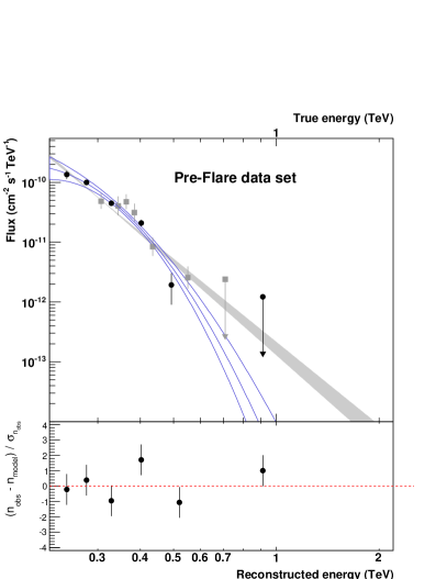
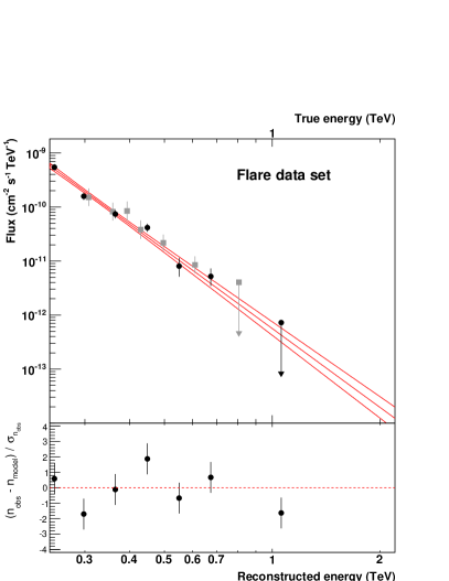
Figure 1: Differential fluxes of PG 1553+113 during the pre-flare (left) and
flare (right) periods. Error contours indicate the 68 % uncertainty on the spectrum.
Uncertainties on the spectral points (in black) are given at level, and upper
limits are computed at the 99 % confidence level. The gray squares were
obtained by the cross-check analysis chain and are presented to visualize the match between both
analyses. The gray error contour on the left panel is the best-fit power law
model. The lower panels show the residuals of the fit, i.e. the difference between
the measured () and expected numbers of photons
(), divided by the statistical error on the measured
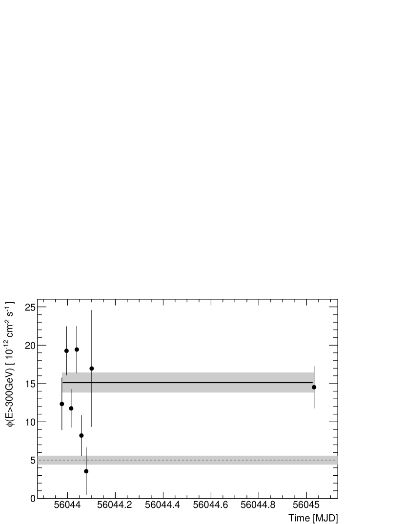
number of photons ().Figure 2: H.E.S.S. light curve of PG 1553+113 during the 2 nights of the flare period. The
continuous line is the measured flux during the flare period while the dashed one
corresponds to the pre-flare period (see Table 2 for the flux values).
Gray areas are the errors.
To compute the light curves, the integrated flux above 300 GeV for each
observation run was extracted using the corresponding (pre-flare or flare)
best fit spectral model. A fit with a constant of the run-wise light curve of the entire (pre-flare+flare)
data set, weighted by the statistical errors yields a of with
d.o.f. (). Restricting the analysis to the pre-flare data set
only, the fit yields a of 51.76 with 60 d.o.f. (),
indicating again a flux increase detected by H.E.S.S. at the time of the flaring activity
reported by Cortina (2012b).
Figure 2 shows the light curve during the flare together with the averaged
integral fluxes above 300 GeV of both data sets. A fit with a constant to the H.E.S.S. light curve during the first night yields a of for d.o.f.
(), indicating intra-night variability. This is also supported by the use of a Bayesian block algorithm (Scargle, 1998) that finds three blocks for the 2 nights at a 95% confidence level.
Table 2: Summary of the fitted spectral
parameters for the pre-flare and the flare data sets and the
corresponding integral flux calculated above 300 GeV. The last column gives the
decorrelation energy.
Data Set (Model)
Spectral Parameters
(E300 GeV)
cm-2 s-1
[GeV]
Pre-Flare (PWL)
306
Pre-Flare (LP)
Flare (PWL)
327
2.2 Fermi-LAT analysis
The Fermi Large Area Telescope (LAT) is detector converting ray to pairs
(Atwood et al., 2009). The LAT is
sensitive to rays from 20 MeV to GeV. In survey mode, in which the bulk of
the observations are performed, each source is seen every 3 hours for
approximately 30 minutes.
The Fermi-LAT data and software are available from the Fermi Science Support
Center444http://fermi.gsfc.nasa.gov/ssc/data/analysis/. In this
work, the ScienceTools V9R32P5 were used with the Pass 7 reprocessed data
(Bregeon et al., 2013), specifically SOURCE class event
(Ackermann et al., 2012a), with the associated P7REP_SOURCE_V15
instrument response functions (IRFs). Events with energies from 300 MeV to
300 GeV were selected. Additional cuts on the zenith angle () and
rocking angle () were applied as recommended by the LAT
collaboration555http://fermi.gsfc.nasa.gov/ssc/data/analysis/documentation/Cicerone/index.html
to reduce the contamination from the Earth atmospheric secondary radiation.
The analysis of the LAT data was performed using the Enrico Python package
(Sanchez & Deil, 2013). The sky model was defined as a region of interest
(ROI) of radius with PG 1553+113 in the center and additional point-like
sources from the internal 4-years source list. Only the sources within a 3∘ radius around PG 1553+113 and bright sources (integral flux greater that ph cm-2 s-1) had their parameters free to vary during
the likelihood minimization. The template files
isotrop_4years_P7_V15_repro_v2_source.txt for the
isotropic diffuse component, and template_4years_P7_v15_repro_v2.fits for the standard Galactic model, were
included. A binned likelihood analysis (Mattox et al., 1996), implemented
in the gtlike tool, was used to find the best-fit parameters.
As for the H.E.S.S. data analysis, two spectral models were used: a simple PWL and
a LP. A likelihood ratio test was used to decide which model best describes the
data. Table 3 gives the results for the two time periods considered
in this work, and Figure 3 presents the -ray SEDs. The first one
(pre-flare), before the H.E.S.S. exposures in 2012, includes more than 3.5 years
of data (from 2008 August 4 to 2012 March 1). The best fit model is found to be
the LP (with a TS666Here the TS is 2 times the difference between the
log-likelihood of the fit with a LP minus the log-likelihood with a PL. of
11.3, ). The second period (flare) is centered on the H.E.S.S. observations windows and lasts for seven days. The best fit model is a power
law, the flux being consistent with the one measured during the first 3.5 years.
Data points or light curves were computed within a restricted energy range or
time range using a PWL model with the spectral index frozen to 1.70.
To precisely probe the variability in HE rays, seven-day time bins were
used to compute the light curve of PG 1553+113 in an extended time window (from 2008
August 4 to 2012 October 30), to probe any possible delay of a HE flare with
respect to the VHE one. While the flux of PG 1553+113 above 300 MeV is found to be variable
in the whole period with a variability index of (Vaughan et al., 2003),
there is no sign of any flaring activity
around the 2012 H.E.S.S. observations. This result has been confirmed by using the
Bayesian block algorithm, which finds no block
around the H.E.S.S. exposures in 2012. Similar results were obtained when
considering only photons with an energy greater than 1 GeV. No sign of
enhancement of the HE flux associated to the VHE event reported here was found. This might be due to the lack of statistic at high energy in the LAT energy range.
Table 3: Results of the Fermi-LAT data analysis for the pre-flare and flare periods.
For the latter, the analysis has been performed in two energy ranges (see 3.2).
The first columns give the time and energy windows
and the third the corresponding test statistic (TS) value. The model
parameters and the flux above 300 MeV are given in the last columns. The systematic uncertainties were computed
using the IRFs bracketing method (Abdo et al., 2009a).
MJD range
Energy range
TS
Spectral Parameters
(EMeV)
[GeV]
[ph cm-2 s-1]
54682-55987
0.3-300
7793.7
56040-56047
0.3-300
43.8
56040-56047
0.3-80
44.5
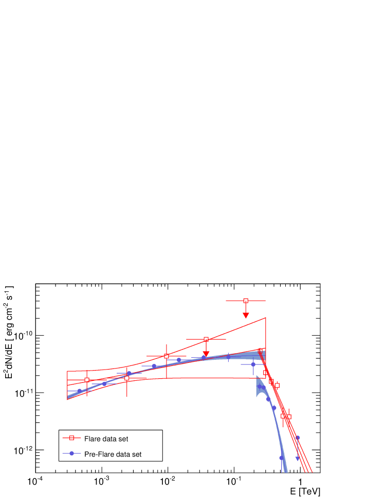
Figure 3: Spectral energy distribution of PG 1553+113 in rays as measured by the Fermi-LAT and H.E.S.S. Red (blue)
points and butterflies have been obtained during the flare (pre-flare) period. The Fermi and H.E.S.S. data for the pre-flare are not contemporaneous. H.E.S.S. data were taken in 2005-2006 while the Fermi data were taken between 2008 and 2012.
3 Discussion of the results
3.1 Variability in -rays
The VHE data do not show any sign of variation of the spectral index (when
comparing flare and pre-flare data sets with the same spectral model), and in HE no counterpart of this event can be found. The indication for intra-night
variability is similar to other TeV HBLs (Mrk 421, Mrk 501 or PKS 2155-304) with,
in this case, flux variations of a factor 3.
As noticed in previous works, PG 1553+113 presents a sharp break between the HE and VHE
ranges (Abdo et al., 2010a) and the peak position of the -ray
spectrum in the
representation is located around 100 GeV. This is confirmed by the fact that the
log-parabola model better represents the pre-flare period in HE. Nonetheless,
the precise location of this peak cannot be determined with the Fermi-LAT data only.
Combining both energy ranges and fitting the HE and VHE data points with a power
law with an exponential cutoff777A fit with a LP model has been attempted, but
the power law with an exponential cutoff leads to a better description of the data.
allows us to determine the peak position for both time periods. The functional form of the model is
For this
purpose, Fermi-LAT and H.E.S.S. systematic uncertainties were taken into account in a
similar way as in Abramowski et al. (2014) and added quadratically to the statistical errors.
The Fermi-LAT systematic uncertainties
were estimated by Ackermann et al. (2012a) to be 10 % of the effective area at
100 MeV, 5 % at 316 MeV and 15 % at 1 TeV and above. For
the VHE -ray range, they were taken into account by shifting
the energy by 10 %. This effect translates into a systematic
uncertainty for a single point of where is the differential flux at energy .
The results of this parameterization are given in Table 4. Using the
pre-flare period, the peak position is found to be located at with no evidence of
variation during the flare and no spectral variation. This is
consistent with the fact that no variability in HE rays was found
during the H.E.S.S. observations. This is also in agreement with the fact that
HBLs are less variable in HE rays than other BL Lac objects
(Abdo et al., 2010b), while numerous flares have been reported in the TeV
band.
Table 4: Parametrization results of the two time periods (first
column) obtained by combining H.E.S.S. and Fermi-LAT. The second column gives the
normalization at 100 GeV, while the third
and the fourth present the spectral index and cut-off energy of the fitted power
law with an exponential cut-off. The last column is the peak energy in a representation.
Period
N (=100 GeV)
[]
Pre-Flare
Flare
3.2 Constraints on the redshift
The extragalactic background light (EBL) is a field of UV to far infrared
photons produced by the thermal emission from stars and reprocessed starlight
by dust in galaxies (see Hauser & Dwek, 2001, for a review) that interacts with
very high energy rays from sources at cosmological distances. As a consequence, a
source at redshift exhibits an observed spectrum where is the intrinsic source
spectrum and is the optical depth due to interaction with the EBL. Since
the optical depth increases with increasing -ray energy, the integral
flux is lowered and the spectral index is
increased888For sake of simplicity it is assumed here that the best-fit
model is a power law, an assumption which is true for most of the cases due to
limited statistics in the VHE range. In the following, the model of
Franceschini et al. (2008) was used to compute the optical depth as a
function of redshift and energy. In this section, the data taken by both
instruments during the flare period are used, with the Fermi-LAT analysis restricted
to the range 300 MeV80 GeV (see Table 3 for the results). In the modest redshift range of VHE emitters detected so
far (), the EBL absorption is negligible below 80 GeV ( at 80 GeV for ).
A measure of the EBL energy density was obtained by Ackermann et al. (2012b) and
Abramowski et al. (2013b) based on the spectra of sources with a known . In
the case of PG 1553+113, for which the redshift is unknown, the effects of the EBL on
the VHE spectrum might be used to derive constraints on its distance. Ideally,
this would be done by comparing the observed spectrum with the intrinsic one but
the latter is unknown. The Fermi-LAT spectrum, derived below 80 GeV, can be
considered as a proxy for the intrinsic spectrum in the VHE regime, or at least, as
a solid upper limit (assuming no hardening of the spectrum).
Following the method used by Abramowski et al. (2013a), it has been assumed
that the intrinsic spectrum of the source in the H.E.S.S. energy range cannot be
harder than the extrapolation of the Fermi-LAT measurement. From this,
one can conclude that the optical depth cannot be greater than ,
given by:
(1)
where is the extrapolation of the Fermi-LAT
measurement towards the H.E.S.S. energy range. is the measured flux by H.E.S.S. The factor accounts
for the systematic uncertainties of the H.E.S.S. measurement and the number 1.64
has been calculated to have a confidence level of 95%
(Abramowski et al., 2013a). The comparison is made at the H.E.S.S. decorrelation
energy where the flux is best measured.
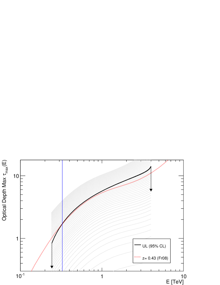
Figure 4: Values of as a function of the photon energy. The
black line is the 95% UL obtained with the H.E.S.S. data and the red line is
the optical depth computed with the model of Franceschini et al. (2008) for a
redshift of 0.43. The blue line is the decorrelation energy fo the H.E.S.S. analyse. The gray lines are the value of optical depth for different redshift.
Figure 4 shows the 95 % UL on . The resulting
upper limit on the redshift is . This method does not
allow the statistical and systematic uncertainties of the Fermi-LAT measurement to
be taken into account and does not take advantage of the spectral features of
the absorbed spectrum (see Abramowski et al., 2013b).
A Bayesian approach has been developed with the aim of taking all the
uncertainties into account. It also uses the fact that
EBL-absorbed spectra are not strictly power laws. The details of the model are
presented in Appendix A and only the main assumptions and results are
recalled here. Intrinsic curvature between the HE and VHE ranges that naturally
arises due to either curvature of the emitting distribution of particles or
emission effects (e.g. Klein-Nishina effects) is permitted by construction of
the prior (Eq. A1): A spectral index softer than the Fermi-LAT measurement is allowed with a constant probability, in contrast with the
previous calculation. It is assumed that the observed spectrum in VHE
rays cannot be harder than the Fermi-LAT measurement by using a prior that
follows a Gaussian for indices harder than the Fermi-LAT one. The prior on the index is then:
(2)
if and
otherwise.
is the index measured by Fermi-LAT and is the
uncertainty on this measurement that takes all the systematic and statistical
uncertainties into account.
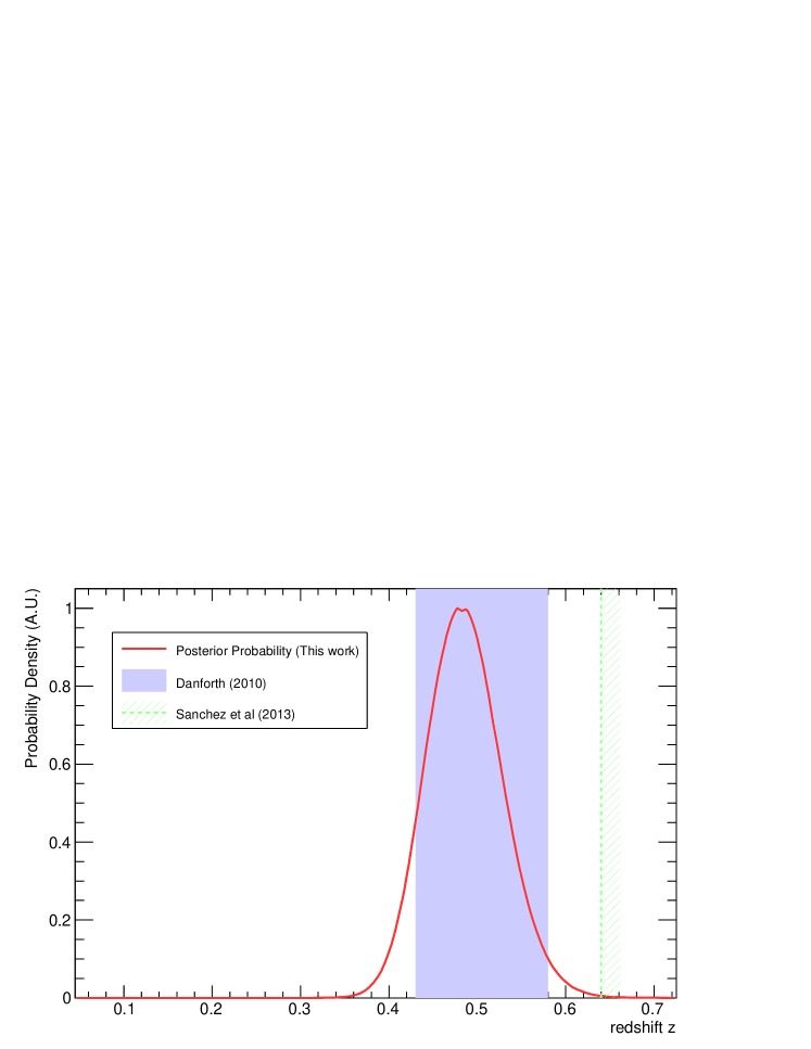
Figure 5: Posterior probability density as a function of redshift (red). The blue area
represents the redshift range estimated by Danforth et al. (2010) while the
green dashed line indicates the limit of Sanchez et al. (2013).
The most probable redshift found with this method is , in good agreement
with the independent measure of Danforth et al. (2010), who constrained
the distance to be between . Figure 5 gives the
posterior probability obtained with the Bayesian method compared with other
measurements of . Lower and upper limits at a confidence level of 95 % can
also be derived as . Note that this method allows the systematic
uncertainties of both instruments (Fermi-LAT and H.E.S.S.) to be taken into account. The spectral index obtained when fitting the H.E.S.S. data with an EBL absorbed PWL using a redshift of 0.49 is compatible with the Fermi measurement below 80 GeV.
3.3 Lorentz Invariance Violation
As stated in section 2.1, the H.E.S.S. data of the flare show a indication of intra-night variability, which is used here to test for a possible Lorentz Invariance Violation (LIV). Some Quantum Gravity (QG) models predict a change
of the speed of light at energies close to the Planck scale ( GeV). A review of such models can be found in
Mattingly (2005) and Liberati (2013). An energy-dependent
dispersion in vacuum is searched for in the data by testing a correlation
between arrival times of the photons and their energies. For two photons with
arrival times and and energies and , the dispersion
parameter of order is defined as . Here only the linear (n = 1)
and quadratic (n = 2) dispersion parameters are calculated. Assuming no
intrinsic spectral variability of the source, the dispersion can be
related to the normalized distance of the source corrected for the
expansion of the Universe and an energy at which Quantum Gravity
effects are expected to occur (Jacob & Piran, 2008):
(3)
where H0 is the Hubble constant and = 1 (resp. +1) in
the superluminal (resp. subluminal) case, in which the high-energy photons
arrive before (resp. after) low-energy photons. The normalized distance is
calculated from the redshift of the source and the cosmological parameters
, given in the introduction:
(4)
Using the central value of determined in section 3.2, the distance f
or n = 1 and 2 is and .
First, the dispersion measurement method will be described. It will then be applied to
the H.E.S.S. flare dataset (MC simulations and original dataset), in order to measure the
dispersion and provide 95 % 1-sided lower and upper limits on the dispersion parameter
. These limits on will lead to lower limits on using
equation 3.
3.3.1 Modified maximum likelihood method
A maximum likelihood method, following Martinez & Errando (2009), was used to
calculate the dispersion parameter . Albert et al. (2008) applied
this method to a flare of Mkn 501, while Abramowski et al. (2011)
applied it to a flare of PKS 2155-304. More recently, it was used by
Vasileiou et al. (2013) to analyse Fermi data of four gamma-ray bursts.
The data from Cherenkov telescopes is contaminated by decay from proton showers,
misidentified electrons, or heavy
elements such as helium. In the case of PG 1553+113, and contrary to previous analyses, this
background is not negligible: the signal-over-background ratio S/B is about 2, compared
to 300 for the PKS 2155–304 flare event of July 2006 (Aharonian et al., 2007b).
The background was included in the formulation of the probability density function
(PDF) used in a likelihood maximization method.
Given the times and energies of the gamma-like (ON) particles received
by the detector, the unbinned likelihood, function of the dispersion parameter is:
(5)
The PDF associated with each ON
event is composed of two terms:
(6)
with
(7)
(8)
(9)
The PDF includes the emission time distribution of the photons
determined from a parametrization of the observed light curve
at low energies (discussed in the next section) and evaluated on
to take into account the delay due to a possible LIV effect, the measured signal spectrum
and the effective area .
The PDF is composed of the uniform time distribution
of the background events, the measured background spectrum and the
effective area . No delay due to a possible LIV effect is expected in the background
events of the ON data set.
and are the normalization factors of and
respectively, in the (, ) range of the likelihood fit.
The coefficient corresponds to the relative weight of the signal events in the
total ON data set, derived from the number of events in the ON region and
the number of events in the OFF regions weighted by the inverse number of
OFF regions . More details on the derivation of this function are given in
Appendix B.1.
3.3.2 Specific selection cuts and timing model
The flare data set of the H.E.S.S. analysis (see section 2.1) was used with
additional cuts. To perform the dispersion studies, only uninterrupted data have been
kept. Thus, the analysis was conducted on the first 7 runs, taken during the night of
April 26th. Moreover, the cosmic ray flux increases substantially for the 7th run, due
to a variation of the zenith angle during this night. This fact, along with its large
statistical errors, leads us to discard this run from the analysis. The 6th run
shows little to no variability and was therefore also removed from the LIV analysis.
Since within the ON data set, the signal and the background spectra have different
indices ( for the signal and
for the background),
the ratio S/B is expected to decrease with increasing energy. An upper
energy cut at = 789 GeV was set, corresponding to the last
bin with more than significance in the reconstructed photon spectrum (see
the differential flux during the flare in Fig. 1).
A lower cut on the energy at = 300 GeV was used in order to avoid large
systematic effects arising from high uncertainties on the H.E.S.S. effective area at lower energies.
The intrinsic light curve of the flare, needed in the formulation of the likelihood, can be
obtained from a model of the timed emission or approximated from a subset of the data. To be
as model-independent as possible, it was here derived from a fit of the measured light curve
at low energies (with ).
The high-energy events () were processed in the calculation of the likelihood
to search for potential dispersion. Here was set to = 400 GeV,
which is approximately the median energy of the ON event sample. Other cuts on the energy
did not introduce significant effects on the final results.
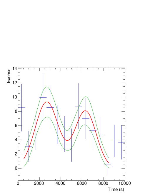
The histogram and the fit (Fig. 6) were obtained as follows: the main idea was to preserve the
maximum detected variability in the PG 1553+113 flare, together with a significant response in
each observed peak:
•
The binning was chosen so that at least two adjacent bins of the
distribution yield a minimum of excess with respect to the average value.
•
Simple parameterization have been tested on the whole data set (all
energies): constant (/d.o.f=25/12), single Gaussian
(/d.o.f=20/10) and double Gaussian (/d.o.f=8.5/7) functions.
The latter is preferred, since it improves the quality of the fit. This shape
was chosen to fit the low energy subset of events. Choosing a single Gaussian
parametrization would result in a decrease of the sensitivity to time-lag
measurements by a factor of two.
Figure 6: Time distribution of the excess in the first 6 runs (70971-70976),
with energies between 300 GeV and 400 GeV.
T = 0 corresponds to the time of the first detected event in run 70971.
The vertical bars correspond to statistical errors; the horizontal bars
correspond to the bin width in time. The best fit, in red, was used as the template light
curve in the maximum likelihood method; the error envelope is shown in green.
There is a gap of 2 min between each two consecutive runs. We did not
consider the effect of these gaps as it is small with respect to the bin width
of 10 min. More importantly, their occurrence is not correlated with
the binning: one gap falls in the rising part of the light curve, one is at a
maximum, two fall in the decreasing parts and none of the gaps is at the
minimum.
Table 6 in Appendix B.2 shows the number of ON and OFF events
for the different cuts applied to the data.
3.3.3 Results: limits on and
The maximum likelihood method was performed using high-energy events with .
First, confidence intervals (CIs) corresponding to 95 % confidence level (1-sided)
were determined from the likelihood curve at the values of where the curve
reaches 2.71, which corresponds to the 90% C.L. quantile of a distribution.
However, these CIs are derived from one realization only and do not take into account
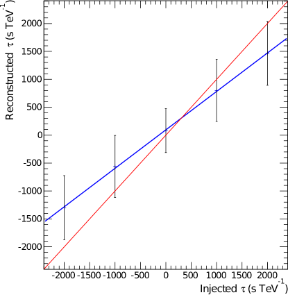
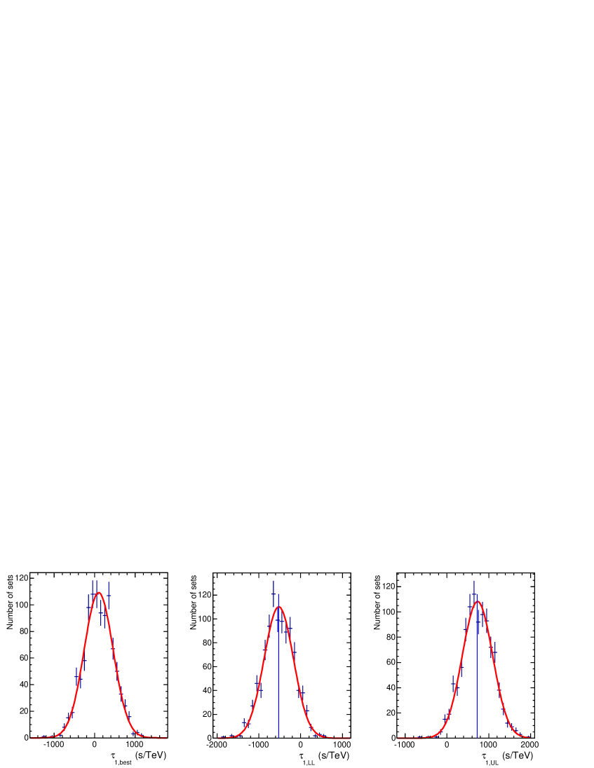
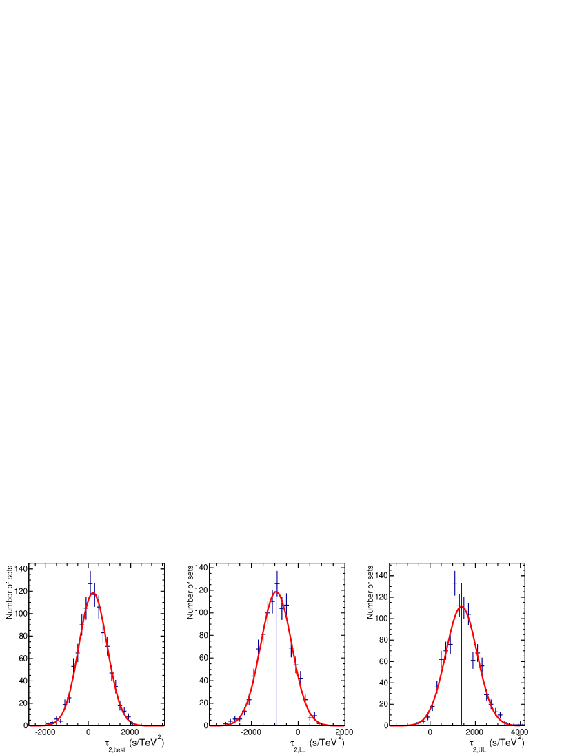
the “luckiness” factor of this measurement. To get statistically
significant CIs (“calibrated CIs”), several sets were generated with Monte Carlo
simulations, with the same statistical significance, light curve model and
spectrum as the original data set. No intrinsic dispersion was artificially
added. Each simulated data set produces a lower limit and an upper limit on
. The calibrated lower (upper) limit of the confidence interval is
obtained from the mean of the distribution of the per-set individual lower (upper)
limits.
Both confidence intervals (from the data only and from the simulated sets) are
listed in Table
7. Sources of systematic errors include uncertainties on the light
curve parameterization, the background contribution, the calculation of the effective
area, the energy resolution, and the determination of the photon index (see Appendix
B.4).
Table 5: Calibrated 95% 1-sided LL and UL (including systematic errors) on
the dispersion parameter and derived 95% 1-sided lower limits on .
Limits on (s TeV-n)
Lower limits on (GeV)
n
s
s
1
-838.9
576.4
2.83 1017
4.11 1017
2
-1570.5
1012.4
1.68 1010
2.10 1010
The resulting limits on the dispersion using the quadratic sum of
the statistical errors from the simulations and the systematic errors
determined from data and simulations were computed,
leading to limits on the energy scale (Eq. 3).
The 95 % 1-sided lower limits for the subluminal case (s = +1) are:
GeV and GeV for linear and quadratic LIV effects,
respectively. For the superluminal case (s = –1) the limits are: GeV and GeV
for linear and quadratic LIV effects, respectively.
Fig. 7 shows a comparison of the different lower limits on
and for the subluminal case (s = +1)
obtained with AGN at different redshifts studied at very high energies.
All these limits, including the present results, have been obtained under the
assumption that no intrinsic delays between photons of different energies occur
at the source. For the linear/subluminal case, the most constraining limit on with transient astrophysical events has been obtained with GRB 090510: GeV (Vasileiou et al., 2013). The most constraining limits on with AGN so far have
been obtained by Abramowski et al. (2011) with PKS 2155-304 data observed
with H.E.S.S.: GeV and
GeV for linear and
quadratic LIV effects, respectively (95% CL, 1-sided).
Compared to the PKS 2155-304 limits, the limits on the linear dispersion for PG 1553+113 are one order of magnitude less constraining, but the limits on the quadratic
dispersion are of the same order of magnitude since the source is located at a higher
redshift. This highlights the interest in studying distant AGN, in spite of the
difficulties due to limited photon statistics.
Figure 7: Lower limits on from linear dispersion (left)
and on from quadratic dispersion (right) for the subluminal
case (s = +1) obtained with
AGN as a function of redshift. The limits are given in terms of .
The constraints from Mkn 421 have been obtained by Biller et al. (1999), from
Mkn 501 by Albert et al. (2008),
and from PKS 2155-304 by Abramowski et al. (2011).
4 Conclusions
A VHE -ray flaring event of PG 1553+113 has been detected with the H.E.S.S. telescopes,
with a flux increasing of a factor of 3. No variability of the spectral index has been
found in the data set, but indication of intra-night flux variability is reported in this
work. In HE rays, no counterpart of this event can be identified, which may be
interpreted as the sign of injection of high energy particles emitting predominantly in
VHE rays. Such particles might not be numerous enough to have a significant
impact on the HE flux during either their acceleration or cooling phases.
The data were used to constrain the redshift of the source using a new approach based
on the absorption properties of the EBL imprinted in the spectrum of a distant source.
Taking into account all the instrumental systematic uncertainties, the redshift of PG 1553+113 is determined as being .
Flares of variable sources can be used to probe LIV effects,
manifesting themselves as an energy-dependent delay in the photon arrival time. A
likelihood method, adapted to flares with a large amount of background and
modest statistics, was presented. To demonstrate the analysis power of this
method, it was applied to the H.E.S.S. data of a flare of PG 1553+113. This analysis
relies on the indication of the intra-night variability of the flare at VHE.
No significant dispersion was measured, and limits on the
scale were derived, in a region of redshift unexplored until now.
Limits on the energy scale at which
QG effects causing LIV may arise, derived in this work, are GeV and GeV for the subluminal
case. Compared with previous limits obtained with the PKS 2155-304 flare of 2006 July, the
limits for PG 1553+113 for a linear dispersion are one order of magnitude less constraining while
limits for a quadratic dispersion are of the same order of magnitude. With the new telescope
placed at the center of the H.E.S.S. array that provides an energy threshold of several tens
of GeV, a better picture of the variability patterns of AGN flares should be obtained.
The future Cherenkov Telescope
Array (CTA) will increase the number of flare detections (Sol et al., 2013)
with better sensitivity, allowing for the extraction of even more constraining limits
on the LIV effects.
Acknowledgements
The support of the Namibian authorities and of the University of Namibia in
facilitating the construction and operation of H.E.S.S. is gratefully
acknowledged, as is the support by the German Ministry for Education and
Research (BMBF), the Max Planck Society, the French Ministry for Research, the
CNRS-IN2P3 and the Astroparticle Interdisciplinary Programme of the CNRS, the
U.K. Particle Physics and Astronomy Research Council (PPARC), the IPNP of the
Charles University, the South African Department of Science and Technology and
National Research Foundation, and by the University of Namibia. We appreciate
the excellent work of the technical support staff in Berlin, Durham, Hamburg,
Heidelberg, Palaiseau, Paris, Saclay, and in Namibia in the construction and
operation of the equipment.
The Fermi LAT Collaboration acknowledges generous ongoing support from a number of agencies and institutes that have supported both the development and the operation of the LAT as well as scientific data analysis. These include the National Aeronautics and Space Administration and the Department of Energy in the United States, the Commissariat à l’Energie Atomique and the Centre National de la Recherche Scientifique / Institut National de Physique Nucléaire et de Physique des Particules in France, the Agenzia Spaziale Italiana and the Istituto Nazionale di Fisica Nucleare in Italy, the Ministry of Education, Culture, Sports, Science and Technology (MEXT), High Energy Accelerator Research Organization (KEK) and Japan Aerospace Exploration Agency (JAXA) in Japan, and the K. A. Wallenberg Foundation, the Swedish Research Council and the Swedish National Space Board in Sweden.
Additional support for science analysis during the operations phase is gratefully acknowledged from the Istituto Nazionale di Astrofisica in Italy and the Centre National d’Etudes Spatiales in France.
DS work is supported by the LABEX grant enigmass. The authors want to thanks F. Krauss for her useful comments.
Appendix A Bayesian model used to constrain the redshift
A Bayesian approach has been used to compute the redshift value of PG 1553+113 in Section 3.2. The
advantage of such a model is that systematic uncertainties, which are important in
Cherenkov astronomy, can easily be included in the calculation. In the
following, the notation for the model parameters and for the data
set is adopted. All normalization constants are dropped in the development
of the model, and the final probability is normalized at the end.
Bayes’ Theorem, based on the conditional probability rule, allows us to write
the posterior probability for the model parameters as the
product of the likelihood and the prior probability :
The likelihood is the quantity that is maximized during determination of the best-fit
spectrum (Piron et al., 2001). It is at this step that the H.E.S.S. data,
taken during the flare, were actually used. The spectrum model here is a simple
power law corrected for the EBL absorption:
The model parameters are then , and .
The prior is the most difficult and most interesting part of the model. To
derive it, and are assumed to be independent from each other and
independent of the redshift. In contrast, the prior on the redshift might
depend on and . Then, the prior can be simplified using the
conditional probability rule:
As much as possible, weak assumptions should be made to write a robust prior then
often flat (i.e. const) are used. Priors should also be based
on a physical meaning and not contradict the physical and observed properties of
the objects. For the purpose of this model, the prior on is assumed to be
flat and the prior on the spectral index is a truncated Gaussian
) if
and const otherwise. The values of
and are
obtained by analyzing LAT data below 80 GeV (see section 3 and
Table 3). Here, it is assumed that the intrinsic spectrum in the
VHE range cannot be harder than the Fermi-LAT measurement. takes
into account the statistical and systematic uncertainties on the Fermi-LAT measurement and also the systematic uncertainty on the H.E.S.S. spectrum
(, see Aharonian et al., 2006b) added quadratically and
for a mean value of .
The prior on is much more difficult to determine. A flat prior has no physical
motivations since the probability to detect sources at TeV energy decreases with
the redshift. The number of sources detected at TeV energy is not sufficient to
use the corresponding redshift distribution as a prior.
A prior which takes into account the EBL, can be derived assuming a
population of sources with a constant spatial density. In the small
space element , the number of such sources scales .
For any given luminosity, their flux (which scales with the probability to detect
them) is scaled by . Lacking a proper knowledge of the
intrinsic luminosity function of VHE -ray blazars, a reasonable
assumption on the detection probability of a blazar at any redshift is
a scaling proportional to the flux for a given luminosity, i.e., .
Putting everything together, the prior on the redshift reads
Finally, the prior we use for our analysis is:
(A1)
if and
otherwise. Putting all the components of the model
together and marginalizing over the nuisance parameters and , the probability
on the redshift can be computed numerically. The
obtained mean value is . At a confidence level of 95 %, the redshift is
between .
In this work, only the model of Franceschini et al. (2008) has been used. Other EBL
models available in the literature predict slightly different absorption depths.
This will lead to a small difference in the redshift. The use
of a flat prior for the redshift distribution of the sources or a prior based on
estimates of the HBLs luminosity function (Ajello et al., 2014) leads to
changes of order of 0.01 on the resulting redshift.
Appendix B Development of the LIV method
B.1 Modified maximum likelihood method
In previous LIV studies with AGN flares (Albert et al., 2008; Abramowski et al., 2011)
the signal was clearly dominating
over the background, whereas in the present study the signal-over-background ratio is about 2.
The background has been included in the formulation of the probability density function (PDF):
in the most general case, for given numbers of signal and background events and in the
observation region (“ON” region), for a given dispersion parameter , the unbinned
likelihood is:
(B1)
The PDF associated with each gamma-like
particle characterized by its time and energy contains two terms (signal and background):
(B2)
with
(B3)
is the number of events detected in the source ON region included in the fit
range .
is the number of events in the OFF regions, in the same (, ) range; is
the inverse number of OFF regions. () is the Poisson
distribution with index () and parameter ().
The likelihood function can be simplified by fixing and from a comparison of
ON and OFF sets: and .
In this case, the Poisson terms in Eq. B2 are equal to 1.
The probabilities and are defined as:
(B4)
(B5)
with
(B6)
(B7)
is the probability that the event
(, ) is a photon emitted at the source and detected on Earth
with a delay . It takes into account the emission
(time distribution and energy spectrum
at the source), the propagation
(delay due to possible LIV effect) and the detection of a
photon by the detector (H.E.S.S. energy resolution and effective
area ).
is the probability that the event (, ) is
a background event; it is not expected to be variable with time, thus
is a uniform time distribution: .
The background energy distribution is measured from OFF regions.
(resp. ) is the normalization factor of the PDF
(resp. ) in the range where the likelihood fit is performed.
Also, the energy resolution is assumed to be perfect in the range
999The actual energy resolution is of the order
of 10 % in this range..
This leads to simplified expressions of and
:
(B8)
(B9)
The best estimate of the dispersion parameter is obtained by maximizing
the likelihood .
B.2 Selection cuts
Table 6 shows the effect of the selection cuts on the number of ON and OFF events.
Other choices of and did not introduce significant changes in the
final results.
Table 6: Selections applied to the ON and OFF data sets
Selection
# of ON events
Weighted # of OFF events
S/B
Total sample
461 (100 %)
144.3 (100 %)
2.2
(1) = Time in 500–8500 s
358 (77.7 %)
95.8 (66.4 %)
2.7
(1) and in 0.3–0.789 TeV
154 (33.4 %)
36.3 (25.1 %)
3.2
(1) and in 0.3–0.4 TeV (Template)
82 (17.8 %)
14.2 (9.9 %)
4.8
(1) and in 0.4–0.789 TeV (LH fit)
72 (15.6 %)
21.9 (15.2 %)
2.3
B.3 Test of the method, confidence intervals
The method has been tested on Monte Carlo (MC) simulated sets. Each set was composed of
ON events, as in the real data sample:
•
signal events with times following the template light curve (Fig. 6)
shifted by a factor ; energies follow a power law spectrum
of photon index , degraded by the acceptance and convolved with
the energy resolution.
•
background events with times following a uniform distribution and energies
drawn from a power law spectrum of index , degraded by the
acceptance and convoluted by the energy resolution.
For a given injected dispersion, the maximum likelihood method is applied to each
MC-simulated set.
The initial light curve and energy spectrum were used as templates in the model instead
of fitting them for each set.
Figure 8 shows the means of the reconstructed dispersion versus
the real (injected) dispersion for n = 1; for a given injected dispersion, error
bars correspond to the RMS of the distribution of the best estimates . The
blue line shows the result of a linear fit.
The slope roughly corresponds to the percentage of signal in the total ON data set.
It is due to the loss of sensitivity resulting from the part of the data sets with no dispersion.
A systematic shift is observed of about 100 s TeV-1, well bellow 1 value – the
RMS of the best estimate distribution is of 361 s TeV-1. The results in this paper have
not been corrected for this bias.
Figure 8: Means of the reconstructed dispersion versus the real (injected dispersion)
for the linear case n = 1; for a given injected dispersion, errors bars correspond to the means
of the distribution of the upper and lower limits (90 % 2-sided 95 % 1-sided). The
blue line is a linear fit to the points. The red line shows the ideally obtained curve
obtained in the case S/B = .
The coverage is not necessarily proper, i.e. the number of sets for which the
injected dispersion value lies between the set’s lower limit (LL) and
upper limit (UL) does not match the required 95 % 1-sided confidence level.
The common cut used on the likelihood curves to get the LLs/ULs has been iteratively
adjusted to ensure a correct statistical coverage: using this new cut, 95 % of the
realizations provide CIs that include the injected dispersion .
The initial coverage was about 85 % for a cut on of 2.71. The new
common cut, found iteratively at 3.5, ensures the desired 90 % 2-sided CL (approx. 95 % 1-sided CL).
Figure 9 shows the distributions of the best estimates, the 95% 1-sided
LLs and ULs for s TeV-1 (linear case) and
s TeV-2 (quadratic case); the means of the lower
and upper limit distributions, shown as a blue vertical line, are used to construct
the “calibrated confidence interval”.
Figure 9: Distributions of the best estimates, the 95% 1-sided lower and upper limits
from simulations in case of no injected dispersion ( s TeV-n),
for n = 1 (top) and n = 2 (bottom); dispersion values are in s TeV-n.
The blue vertical line on the LL (resp. UL) distribution shows (resp. ),
defined as the mean of the distribution.
To get CIs from data, a maximum likelihood method is applied to the original data set
and gives a best estimate .
The cut value determined from the simulations to ensure proper coverage is applied on
the original data set to obtain and .
The “calibrated” limits and , combining
from data together with MC results, are taken as
(B10)
with , and defined as
the mean of the per-set best-estimate distribution, LL distribution, and UL distribution
respectively.
Table 7 lists the CIs determined in both ways, i.e., data-only and calibrated
ones: and (resp. and )
are compatible within 10 %.
In this work, calibrated CIs have been used to derive the final lower limits on .
They are preferred over data-only CIs as they provides statistically well defined confidence levels.
They also ensure coherent comparison with previous published results, e.g. with PKS 2155–304
by Abramowski et al. (2011) and GRB studies by Vasileiou et al. (2013).
Table 7: Linear (top) and quadratic (bottom) dispersion parameter; from left to right:
best estimate, LL and UL from data (cut on likelihood curve), LL and UL from MC simulations
(means of per-set LL and UL distributions), calibrated LL and UL (combination of data and MC),
calibrated LL and UL including systematic errors. Dispersion parameters , LLs
and ULs are in s TeV-n.
n
with systematics
1
-131.7
-806.7
554.7
99.1
-526.3
725.6
-757.1
494.8
-838.9
576.4
2
-287.5
-1449.9
853.6
217.2
-942.0
1395.0
-1446.7
890.3
-1570.5
1012.4
B.4 Estimation of the systematics
Estimations of the systematic effects on the dispersion measurement were performed. It was
found that the main systematic errors are due to the uncertainties on the light curve
parametrization. Other sources of systematic errors include the contribution of the
background, effect of the change of photon index, the energy resolution and the effective
area determination of the detector.
To study the following four contributions, new simulated data sets have been built,
each one with different input parameters:
•
background contribution: photons and background events have been reallocated
within the ON data set in the fit range , introducing
a fluctuation in the number of signal event in the ON data set;
•
effective area: set to a constant, equal to 120000 m2 for all energies and all
times, which corresponds to a maximum shift of 10 % (the actual effective area increases
with energy);
•
energy resolution: reconstructed energies have been replaced by the true energies;
this corresponds to a shift of about 10 % on the reconstructed energy values;
•
photon index: changed by one standard deviation ().
For the determination of systematic errors arising from the light curve parametrization,
the calibration of the confidence intervals has been redone using successively the upper
and the lower contours of the template, shown in Fig. 6.
The change in mean lower and upper limits on the dispersion parameter gives an
estimate of the systematic error associated to each contribution101010In particular the errors
on the peak positions constitute the most important part of the uncertainty on the template
light curve contributing to the likelihood fit – see previous works, e.g. Abramowski et al. (2011).
Therefore, the covariance matrix of the fit of the template was studied in detail ; the peak positions
were varied by values of extracted from the covariance matrix.
This study led to an increase in overall systematics of the order of 20% for and
40% for , and a decrease of maximum 7% and 2% of limits on
and respectively..
An additional systematic contribution comes from the shift arising from the method found
with simulation (see Appendix B.3).
Table 8 summarizes all studied systematic contributions. The overall estimated
systematic error on is 330 s TeV-1 for the linear case (n = 1) and
555 s TeV-2 for the quadratic case (n = 2); they were included in the
calculation of the limits on EQG by adding the statistical and the systematic errors
in quadrature.
Table 8: Summary of all studied systematic contributions. The main systematic errors
are due to the uncertainties on the light curve parametrization.
Estimated error
on input parameters
(s TeV-1)
(s TeV-2)
Background contribution
Acceptance factors
10%
Energy resolution
10%
Photon index
5%
Light curve parametrization
Systematic bias
Total:
References
Abdo et al. (2009a)
Abdo, A. A., et al. 2009a, ApJ, 707, 1310
Abdo et al. (2009b)
—. 2009b, ApJS, 183, 46
Abdo et al. (2010a)
—. 2010a, ApJ, 708, 1310
Abdo et al. (2010b)
—. 2010b, ApJ, 722, 520
Abramowski et al. (2011)
Abramowski, A., et al. 2011, Astroparticle Physics, 34, 738
Abramowski et al. (2013a)
Abramowski, A., et al. 2013a, A&A, 552, A118
Abramowski et al. (2013b)
—. 2013b, A&A, 550, A4
Abramowski et al. (2014)
—. 2014, Ap Librae paper Submitted to A&A
Ackermann et al. (2012a)
Ackermann, M., et al. 2012a, ApJS, 203, 4
Ackermann et al. (2012b)
—. 2012b, Science, 338, 1190
Aharonian et al. (2006a)
Aharonian, F., et al. 2006a, A&A, 448, L19
Aharonian et al. (2006b)
—. 2006b, A&A, 457, 899
Aharonian et al. (2007a)
—. 2007a, ApJ, 664, L71
Aharonian et al. (2007b)
—. 2007b, ApJ, 664, L71
Aharonian et al. (2008)
—. 2008, A&A, 477, 481
Ajello et al. (2014)
Ajello, M., et al. 2014, ApJ, 780, 73
Albert et al. (2008)
Albert, J., et al. 2008, Physics Letters B, 668, 253
Aleksić et al. (2012)
Aleksić, J., et al. 2012, ApJ, 748, 46
Aleksić et al. (2014)
—. 2014, ArXiv e-prints
Atwood et al. (2009)
Atwood, W. B., et al. 2009, ApJ, 697, 1071
Becherini et al. (2011)
Becherini, Y., Djannati-Ataï, A., Marandon, V., Punch, M., &
Pita, S. 2011, Astroparticle Physics, 34, 858
Berge et al. (2007)
Berge, D., Funk, S., & Hinton, J. 2007, A&A, 466, 1219
Biller et al. (1999)
Biller, S. D., et al. 1999, Physical Review Letters, 83, 2108
Bregeon et al. (2013)
Bregeon, J., Charles, E., & M. Wood for the Fermi-LAT collaboration.
2013, ArXiv 1304.5456
Cortina (2012a)
Cortina, J. 2012a, The Astronomer’s Telegram, 3977, 1
Cortina (2012b)
—. 2012b, The Astronomer’s Telegram, 4069, 1
Danforth et al. (2010)
Danforth, C. W., Keeney, B. A., Stocke, J. T., Shull, J. M., & Yao, Y. 2010,
The Astrophysical Journal, 720, 976
de Naurois & Rolland (2009)
de Naurois, M., & Rolland, L. 2009, Astroparticle Physics, 32, 231
Franceschini et al. (2008)
Franceschini, A., Rodighiero, G., & Vaccari, M. 2008, A&A, 487, 837
Gaidos et al. (1996)
Gaidos, J. A., et al. 1996, Nature, 383, 319
Giommi et al. (1995)
Giommi, P., Ansari, S. G., & Micol, A. 1995, A&AS, 109, 267
Green et al. (1986)
Green, R. F., Schmidt, M., & Liebert, J. 1986, ApJS, 61, 305
Hauser & Dwek (2001)
Hauser, M. G., & Dwek, E. 2001, ARA&A, 39, 249
Hinton & the H.E.S.S. Collaboration (2004)
Hinton, J. A., & the H.E.S.S. Collaboration. 2004, New A Rev., 48, 331
Jacob & Piran (2008)
Jacob, U., & Piran, T. 2008, Journal of Cosmology and Astroparticle Physics,
2008, 031
Komatsu et al. (2011)
Komatsu, E., et al. 2011, The Astrophysical Journal Supplement Series, 192,
18
Li & Ma (1983)
Li, T.-P., & Ma, Y.-Q. 1983, ApJ, 272, 317
Liberati (2013)
Liberati, S. 2013, Classical and Quantum Gravity, 30, 133001
Martinez & Errando (2009)
Martinez, M., & Errando, M. 2009, Astroparticle Physics, 31, 226
Mattingly (2005)
Mattingly, D. 2005, Living Reviews in Relativity, 8
Mattox et al. (1996)
Mattox, J. R., et al. 1996, ApJ, 461, 396
Osterman et al. (2006)
Osterman, M. A., et al. 2006, AJ, 132, 873
Piron et al. (2001)
Piron, F., et al. 2001, A&A, 374, 895
Prandini et al. (2009)
Prandini, E., Dorner, D., Mankuzhiyil, N., Mariotti, M., Mazin, D.,
& for the MAGIC Collaboration. 2009, ArXiv 0907.0157
Rector et al. (2003)
Rector, T. A., Gabuzda, D. C., & Stocke, J. T. 2003, AJ, 125, 1060
Reimer et al. (2008)
Reimer, A., Costamante, L., Madejski, G., Reimer, O., & Dorner, D.
2008, ApJ, 682, 775
Sanchez & Deil (2013)
Sanchez, D. A., & Deil, C. 2013, ArXiv 1307.4534
Sanchez et al. (2013)
Sanchez, D. A., Fegan, S., & Giebels, B. 2013, A&A, 554, A75
Scargle (1998)
Scargle, J. D. 1998, ApJ, 504, 405
Sol et al. (2013)
Sol, H., et al. 2013, Astroparticle Physics, 43, 215
Treves et al. (2007)
Treves, A., Falomo, R., & Uslenghi, M. 2007, A&A, 473, L17
Urry & Padovani (1995)
Urry, C. M., & Padovani, P. 1995, PASP, 107, 803
Vasileiou et al. (2013)
Vasileiou, V., et al. 2013, Physical Review D, 87, 122001
Vaughan et al. (2003)
Vaughan, S., Edelson, R., Warwick, R. S., & Uttley, P. 2003, MNRAS,
345, 1271