Simple model for the Darwinian transition in early evolution

Abstract

It has been hypothesized that in the era just before the last universal common ancestor emerged, life on earth was fundamentally collective. Ancient life forms shared their genetic material freely through massive horizontal gene transfer (HGT). At a certain point, however, life made a transition to the modern era of individuality and vertical descent. Here we present a minimal model for this hypothesized “Darwinian transition.” The model suggests that HGT-dominated dynamics may have been intermittently interrupted by selection-driven processes during which genotypes became fitter and decreased their inclination toward HGT. Stochastic switching in the population dynamics with three-point (hypernetwork) interactions may have destabilized the HGT-dominated collective state and led to the emergence of vertical descent and the first well-defined species in early evolution. A nonlinear analysis of a stochastic model dynamics covering key features of evolutionary processes (such as selection, mutation, drift and HGT) supports this view. Our findings thus suggest a viable route from early collective evolution to the start of individuality and vertical Darwinian evolution.

Keywords: Evolutionary dynamics, population genetics, horizontal gene transfer, early evolution, emergence of the first species, hypernetwork dynamics, Darwinian threshold

I Introduction

I.1 The last universal common ancestor

In the final chapter of “On the Origin of Species”, Charles Darwin speculated that all life on earth may have descended from a common ancestor. As he observed, “all living things have much in common, in their chemical composition, their germinal vesicles, their cellular structure, and their laws of growth and reproduction. $\dots$ Therefore I should infer from analogy that probably all the organic beings which have ever lived on this earth have descended from some one primordial form, into which life was first breathed” Darwin (1859).

A century after Darwin, molecular biology provided new lines of circumstantial evidence for a universal common ancestor. All organisms were found to use the same molecule (DNA) for their genetic material, as well as a canonical look-up table (the genetic code) for translating nucleotide sequences into amino-acid sequences Nirenberg et al. (1963); Woese (1967); Knight et al. (2001). Further clues came from cross-species comparisons of the molecules involved in the most fundamental processes of life, such as protein synthesis, core metabolism, and the storage and handling of the genetic material. The first such analysis Woese and Fox (1977a), based on snippets of ribosomal RNA, provoked a revolution in our understanding of life’s family tree Woese (2000); Ciccarelli et al. (2006); Pace et al. (2012). It indicated that life is divided into three different domains: the Archaea, the Bacteria and the Eucarya Woese and Fox (1977a); Woese (2000); Pace et al. (2012). Later studies using other molecular sequences placed the root of the tree, corresponding to the last universal common ancestor, somewhere between the Bacteria and Archaea Gogarten et al. (1989); Iwabe et al. (1989); Theobald (2010); Dagan et al. (2010); Williams et al. (2013), roughly $3.5-3.8$ billion years ago. The nature of the last universal common ancestor, however, remains unresolved: Was it prokaryotic or eukaryotic? Did it thrive in extreme or moderate temperatures? Was its genome based on RNA or DNA? For a review, see Ref. Glansdorff et al. (2008) and references therein.

I.2 The era of collective evolution

Our work in this paper was inspired by a conjecture proposed by Woese and his colleagues Woese and Fox (1977b); Woese (1998, 2002, 2005). According to this conjecture, the last universal common ancestor was a community, not a single creature. It marked a turning point in the history of life: before it, evolution was collective and dominated by horizontal gene transfer; after it, evolution was Darwinian and dominated by vertical gene transfer.

In Woese’s scenario, life in the epoch leading up to the universal ancestor was intensely communal. It was organized into loose-knit consortia of protocells far simpler than the bacteria or archaea we know today. Woese and Fox  Woese and Fox (1977b) called those hypothetical ancient life forms “progenotes.” The term signifies that the coupling between genotype and phenotype had not yet fully evolved, mainly because the process for translating genes into proteins had not yet fully evolved either. A rudimentary form of translation existed, but it was ambiguous and hence had a statistical character. Instead of producing a single protein, early translation produced a cloud of similar proteins. This ambiguity in protein synthesis in turn limited the specificity of all the progenote’s interactions. For example, lacking the large, complex proteins necessary for accurate copying and repair of the genetic material, the progenote’s genome was tiny and subject to high mutation rates.

Progenotes were not well-defined organisms as such, because they had no individuality and no long-term genetic pedigree. Their genes and component parts could come and go, being swapped in or out with other members of the community via horizontal transfer. But because biochemical innovations produced by any member of the community were available to all, evolution at this time was rapid—probably more rapid than at any time since. Selection acted on whole communities, not on individual progenotes. Those communities that were better at sharing their biochemical breakthroughs flourished. Out of this cauldron of evolutionary innovation, the universal genetic code and its translational machinery co-evolved, in response to the selective pressures favoring efficient sharing and interoperability.

Vetsigian, Woese, and Goldenfeld Vetsigian et al. (2006) confronted and constrained these speculations with mathematical analysis and computer simulations. Going beyond Woese’s conjectures, they probed early evolution scientifically by interpreting the available data on the genetic code. Their dynamical model for the evolution of the genetic code Vetsigian et al. (2006) showed that a collective state of life is required to obtain the observed Haig and Hurst (1991); Freeland and Hurst (1998) statistical properties of the code, in particular, its simultaneous universality and optimality. A later study by Goldenfeld and colleagues Butler et al. (2009) provided further evidence that only a collective state of life could have created the highly optimized code used by all life today  Freeland and Hurst (1998).

I.3 The Darwinian transition

How did the era of collective evolution come to an end? Woese speculated that as the translation process began to improve, and as progenotic subsystems became increasingly complex and specialized, it would have become harder to find foreign parts compatible with them. Thus, horizontal gene transfer would have become increasingly difficult. The only possible modifications at this point would have come from within the progenote’s lineage itself, through mutation and gene duplication. It was in this way that the progenotes would have made the Darwinian transition Woese (2002, 2005) to become “genotes,” i.e., life forms with a tight coupling between their nucleic acid genotypes and their protein phenotypes, and that could therefore evolve through the familiar Darwinian process of vertical descent.

The model considered below is an attempt to explore, in mathematical terms, how the Darwinian transition from the collective state to the modern era of individuality might have taken place. Our approach shares with Ref. Vetsigian et al. (2006) the outlook that a dynamical systems calculation should be devised to support or refute the hypotheses considered. Our results lend support to the proposed collective state of life Woese and Fox (1977b); Woese (1998, 2002, 2005); Vetsigian et al. (2006) by providing a potential mechanism for the exit from that state.

I.4 Horizontal gene transfer

Over the last decades more and more evidence has accumulated that, besides selection, mutation, and drift Drossel (2001), another process drives evolution: horizontal gene transfer. Here we briefly review the main points about horizontal gene transfer relevant to the mathematical model developed below.

While reproduction implies a vertical transfer of genes from one entity to the next in the phylogenetic tree, there are also processes in which possibly unrelated individuals exchange genetic material during their lifetimes, i.e., horizontally in the sense of the tree. This transfer of genes within one generation is consequently termed horizontal gene transfer (HGT) Syvanen (1985, 1994); Delsuc et al. (2005); Thomas and Nielsen (2005) or lateral gene transfer. It is now widely accepted that HGT is a fundamental driving force of evolution Anderson (1966, 1970); Sonea (1988); Syvanen (1994); Kurland et al. (2003); Dagan and Martin (2006); Takeuchi et al. (2014), and that its existence raises profound theoretical problems for evolutionary biology. For example, the longstanding problem of defining bacterial species  Sonea (1988); Cohan (2002); Lawrence (2002); Gevers et al. (2005); Konstantinidis and Tiedje (2005); Staley (2006) is due, in part, to the promiscuous use of HGT by bacteria. A recent primer on horizontal gene transfer and its potential for evolutionary processes in general is given in Zhaxybayeva and Doolittle (2011).

As discussed above, if HGT was rampant in the early stages of evolution, the last universal common ancestor was a community, not a single organism Woese (1998, 2002); Vetsigian et al. (2006); Goldenfeld and Woese (2007). In this collective state, individuals could not yet be distinguished, as each progenote’s genes were frequently exchanged through HGT. In terms of the model to be developed below, the total pool of genotypes in the collective state would be spread out and thus broadly distributed in the state space of all theoretically possible genotypes. Conversely, a genotype distribution that is highly localized in state space, being concentrated on just one or a few genotypes, would be the model’s version of a well-defined species.

Woese postulated that as the collective state of the progenote population slowly evolved toward higher complexity, its rate of HGT slowly decreased Woese (2002). At some point the system crossed the “Darwinian threshold” Woese (2002). Then natural selection instead of HGT started to dominate the dynamics. The fitter individuals were selected for and the first species emerged from the distributed state. In the colorful language of Dyson Dyson (2007):

But then, one evil day, a cell resembling a primitive bacterium happened to find itself one jump ahead of its neighbors in efficiency. That cell, anticipating Bill Gates by three billion years, separated itself from the community and refused to share. Its offspring became the first species of bacteria—and the first species of any kind—reserving their intellectual property for their own private use. With their superior efficiency, the bacteria continued to prosper and to evolve separately, while the rest of the community continued its communal life. Some millions of years later, another cell separated itself from the community and became the ancestor of the archaea. Some time after that, a third cell separated itself and became the ancestor of the eukaryotes.

After making a Darwinian transition, evolution proceeds in the familiar vertical manner, being driven by selection, mutation, and drift Drossel (2001), with HGT playing only a minor role. Such Darwinian dynamics have, of course, been studied extensively in both experimental and model settings Drossel (2001); Taylor et al. (2004); Traulsen et al. (2005); Nowak (2006); Durrett and Schmidt (2008); Arnoldt et al. (2012). Compared to the dynamics of HGT their properties are relatively well understood. Recently, potential influences of HGT on such evolutionary dynamics have been investigated Woese (1998); Vetsigian et al. (2006); Leisner et al. (2008); Moran and Jarvik (2010); Mayer et al. (2011); Vogan and Higgs (2011); Fuentes et al. (2014). Some mathematical models of HGT have focused on how it can increase a population’s fitness in Darwinian evolution Wylie et al. (2010).

Keep in mind, however, that the hypothesized HGT associated with progenotes and the Darwinian transition, being associated with ribosomal genes and the rest of the core machinery of the cell, would have been of far greater evolutionary significance than the HGT of, say, antibiotic resistance genes seen in bacterial communities today. In Woese’s scenario, the ancient form of HGT was rampant, pervasive, and tremendously disruptive and innovative. It was the prime mover in shaping the fabric of the cell Woese (2005).

We would like to understand what such a Darwinian transition would look like, mathematically. The model described in the next section is deliberately minimal. It leaves out all the biology of ribosomes, proteins, genetic codes, and the like. What remains is an attempt to capture the essence of Woese’s speculations. In place of a community of progenotes, we consider a community of abstract genomes, represented by binary sequences. They interact via HGT, and are subject to mutation, selection, and drift on a fitness landscape. Our work suggests that HGT-dominated dynamics may have been intermittently interrupted by selection-driven processes during which genotypes became fitter and decreased their inclination toward HGT. Such stochastic switching in the nonlinear population dynamics may have destabilized the HGT-dominated state and thus led to a Darwinian transition and the emergence of the first species in early evolution.

On a side note, an interesting mathematical aspect of the model is that it necessarily involves three-point interactions, since HGT transforms one genotype into a second by importing pieces of a third. Thus the model provides a natural biological example of a complex hypernetwork. Until now, most models in evolutionary dynamics and population biology did not need to go beyond ordinary network structure, with two-point interactions between nodes connected by links.

II Evolutionary model

To explore the consequences of HGT on evolution, we consider a model community of $N$ progenotes evolving on a fitness landscape Drossel (2001); Wilke et al. (2001) in the presence of selection, mutation, drift, and HGT. Each progenote carries a genome of length $l$ composed of a sequence of the bases $0$ and $1$. The genome of progenote $i$ determines its fitness $f_{i}$. The progenotes reproduce by the Moran process Moran (1962); Drossel (2001), i.e., each progenote reproduces randomly in time, with its reproduction rate given by its fitness $f_{i}$. Whenever a progenote of genotype $i$ reproduces, an offspring is added to the population which is either identical to genotype $i$ or a mutant of genotype $j$ with probability $\mu_{ij}$. Instantaneously after such a reproduction event, one progenote in the population is chosen randomly to die and is hence removed from the population. We assume that one mutation event will only affect one of the bases of the genome, so that the Hamming distance between genotypes $i$ and $j$ is 1.

Hence, our fitness landscape may be represented by a network where the different genotypes are the nodes of the network and the possible mutations form the links. Assigning two different bases, 0 and 1, and given the structure of the mutations, the resulting network is an $l$-dimensional hypercube (Fig. 1).

The fitness landscape underlying our model is assumed to be a Mount Fuji landscape Drossel (2001): The highest fitness is assigned to one single genotype, the peak. Other genotypes are assigned lower fitness: the farther away from the peak in genotype space, the lower the fitness. Thus, a single-peaked mountain landscape is created on genotype space, and a population evolving purely through the processes of selection and mutation should converge to this peak. Note that the Moran process described above is a random process. It thereby constitutes a minimal model intrinsically including the effects of selection, mutation and genetic drift Drossel (2001). The latter is induced by the stochastic selection in the combined process of reproduction, mutation and death and has the effect of randomly walking the population around in genotype space even if no fitness differences were present.

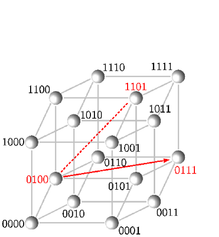
Figure 1: HGT-hyperlinks introduce three-genotype interactions to the evolutionary dynamics, creating hypernetwork dynamics. This schematic example illustrates the insertion of an HGT-hyperlink (red solid and dashed) to the sequence space of genomes of length $l=4$. Individuals of genotype $A=0100$ take up the first two bases $\underline{11}$ from genotype $B=\underline{11}01$ which are inserted at position three into $A=01\underline{11}00$. After the last two bits are cut from the sequence, an progenote of genotype $A$ becomes of new genotype $C=0111$.

To reveal the potential impact of HGT we incorporate its basic features into the stochastic evolution model. Two progenotes $A$ and $B$ may meet and a subsequence $s$ of progenote $B$’s genome may be inserted into $A$’s genome. As a result of this horizontal gene transfer event, the genotype of progenote $A$ will transform into another genotype $C$, determined by its original genotype and the subsequence $s$. This process is illustrated in Figure 1.

To model this process we add HGT-hyperlinks to the hypercube network representing the fitness landscape. One such hyperlink symbolizes a three-genotype interaction and is defined through the following process. We choose two genotypes $A$ and $B$ randomly as well as a random subsequence of genome $B$ with length between $x=2$ and $x=l-2$ bases. This subsequence is inserted at a random position of genome $A$. The remaining $x$ bases at the end of $A$’s sequence are cut off, keeping the sequence length of $A$ constant. The new sequence determines a genotype $C$, which genotype $A$ becomes on interacting with $B$ via this HGT-link, denoted $(\overrightarrow{A,B,C})$. If the resulting genotype $C$ is identical to $A$, this HGT-link would not alter the population dynamics and would thus be irrelevant. We therefore neglect such self-projecting HGT-links. We repeat the above procedure until a predefined number $m$ of new HGT-links has been added to the system.

An HGT-link defines one type of HGT-event, in which part of genotype $A$ is replaced by part of genotype $B$ and is thereby transformed to genotype $C$. We consider these events to occur independently of each other. Let $k_{X}$ denote the number of progenotes of genotype $X$ in the population. Then the HGT-events above occur at a rate

$$r_{A\rightarrow C}^{B}=c\cdot k_{A}\frac{k_{B}}{N}.$$ (1)

Here the effective competence for HGT is modeled as a constant $c\geq 0$ that captures both the rate at which the progenotes meet and their actual preference for the initiation of an HGT event, given that they meet.

Note that interactions of the form (1), independent of any model details, imply collective dynamics on a complex hypernetwork, due to their intrinsic three-genotype coupling involving $A$, $B$, and $C$. The dynamics of horizontal gene transfer in biological systems depends on a multitude of factors, including the mode (e.g., natural transformation or conjugative transfer) of HGT Thomas and Nielsen (2005), and may vary with the fitness of the donor and recipient Leisner et al. (2008, 2009) and other factors such as environmental conditions Kovacs et al. (2009). To focus on qualitative mechanisms, we here consider the simplest setting where $c$ is just a non-negative constant. We note that, via the factors $k_{A}$, $k_{B}$ and the presence or absence of HGT-links $(\overrightarrow{A,B,C})$, the actual rate of all HGT events in the population still depends on how the population is distributed in genotype space.

III Quantifying Stochastic Switching

To see how HGT influences the evolutionary dynamics we study how the collective model dynamics depends on the competence $c$. The population sizes $k_{i}(t)$ of progenotes of different genotypes $i$ present in the population fully describe the state of the system at time $t$. We introduce the population entropy

$$S(t)=-\sum_{i=0}^{2^{l}-1}\frac{k_{i}(t)}{N}\log\left[\frac{k_{i}(t)}{N}\right]$$ (2)

to quantify how broadly the population is distributed in genotype space. Populations consisting of only one genotype have population entropy zero. If the population is uniformly spread out in genotype space, the population entropy takes its maximal value $S_{\text{max}}=l\log(2)$.

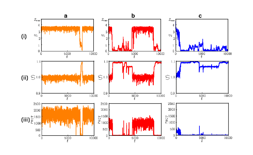
Figure 2: The population dynamics is dominated by a speciated state for low competence and a distributed state for high competence. Shown are example dynamics of the population entropy (2) for competence $c=5$ (a), $c=3$ (b) and $c=1$ (c) in an example population of $N=1000$ progenotes with genome length $l=7$. (a): For high competence $c$ the population entropy almost always fluctuates around a high value for all initial conditions. (b): The dynamics switch stochastically to a low entropy state and stay there longer for lower values of $c$. (c): The low entropy state is rendered globally stable for low $c$ so that the population entropy fluctuates slightly above zero for all initial conditions. In the low entropy state the population dynamics are driven by selection, in the high entropy state by HGT. Panels (i) show the entropy dynamics, (ii) the average fitness $\left\langle f\right\rangle$ of the population corresponding to the entropy dynamics and (iii) the corresponding HGT rates $r_{\text{HGT}}$ that the population exhibits at time $t$. For low population entropies the fitness is high and HGT rate small and vice versa for high population entropies. The mutation probability was set to $\mu_{ij}=0.0001$. Into the resulting Fujiyama fitness landscape Drossel (2001) with fitness values between $f_{\text{min}}=0.9$ and $f_{\text{max}}=1.1$ we inserted $m=2000$ HGT-links.

Direct simulations of the stochastic dynamics reveal that for large competences $c$, the collective dynamics converge to a state of high population entropy where the population is highly spread out in genotype space (Figure 2a). It may only transiently switch to a state localized in state space, i.e., with relatively little spread in genetic material. In this high entropy state the total HGT rate in the population is orders of magnitude higher than in a speciated state (see below). The population does not adapt to the underlying fitness landscape; in that sense, HGT is the main driving process in this large-$c$ scenario. We identify this state of high population entropy with a pre-Darwinian collective state, as in this state no distinct species can be distinguished and HGT is the dominant force driving the evolutionary dynamics.

In contrast, if the progenotes’ competence for HGT is low, we observe a population dynamics which converges toward a state of low population entropy (Figure 2c). This confirms the observation that selection, mutation and drift will drive a population to adapt to a fitness landscape if the mutation rate is not too high Drossel (2001); Nowak (2006). The population is thus concentrated around the fittest genotype with only rare mutations and genetic drift causing some spread of the population. As a consequence, large parts of the population exhibit the same or similar genotypes such that it is in a speciated state.

While the system spends almost all time close to its speciated state for low competence, the dynamics switch stochastically between the speciated and the distributed state if the competence is not small enough. Figures 2a-c show that the higher the progenotes’ competence for HGT is, the longer the system stays in the distributed state.

We conclude that both the speciated state and the distributed state are dynamically accessible metastable states (for high enough competence). The dynamics only switch from one of these states to the other due to rare events in the stochastic dynamics. This is supported by the fact that the dynamics switch between these states on much shorter time scales than the time they remain in them (see also Figure 3 below).

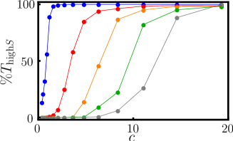
Figure 3: The high entropy state is dynamically stable also for vanishing mutation probabilities. Shown is the measured percentage of time a population stayed in the distributed state for a system with mutation probabilities $\mu_{ij}=10^{-3}$ (blue), $\mu_{ij}=10^{-4}$, $\mu_{ij}=10^{-5}$ (orange), $\mu_{ij}=10^{-6}$ (green) and $\mu_{ij}=0$ (gray). Qualitatively, the results are similar, only for higher mutation probabilities the critical transition occurs at a lower value $c_{\text{cr}}$. System parameters were $l=7$, $N=1000$ and $m=3000$ HGT-links were introduced into a Fujiyama fitness landscape with fitness values between $f_{\text{min}}=0.9$ and $f_{\text{max}}=1.1$. Each datapoint was obtained in a simulation of length $T=10^{6}$ with the initial condition $S(0)=S_{\max}$.

How does the distributed state disappear for low competences? To answer this question we developed a method based on the population entropy defined in (2) to study the forces induced on the dynamics by reproduction and HGT. The evolution dynamics are event-driven, and the population entropy $S$ may only change at these event times. At each event there is a population entropy $S_{-}$ directly before the event and a population entropy $S_{+}$ directly after the event. The change of population entropy

$$\Delta S=S_{+}-S_{-}$$ (3)

induced by a single event will in general depend on the type of event (reproduction or HGT) and the actual distribution of the population over genotype space. If the population is in a state with population entropy $S$, one event will thus induce a mean change $\overline{\Delta S}(S)$ averaged over all events occurring at population entropy $S$. The rate $r(S)$ at which these events occur depends on the state of the system as well. Multiplying the mean change induced by the single events with the rate at which the events occur, we obtain the average rate of change

$$\frac{dS}{dt}=r(S)\cdot\overline{\Delta S}(S)$$ (4)

induced on the dynamics. The reproduction and HGT events in our model occur independently of each other, so that their contributions separate additively according to

$$\frac{dS}{dt} = \frac{dS_{\text{Repr}}}{dt}+\frac{dS_{\text{HGT}}}{dt}$$ (5)

$$= r_{\text{Repr}}(S)\cdot\overline{\Delta S}_{\text{Repr}}(S)+r_{\text{HGT}}(S)\cdot\overline{\Delta S}_{\text{HGT}}(S).$$ (6)

We measured these functional dependencies in simulations of the dynamics (for more details see Supplementary Information), thereby obtaining the forces induced by reproduction and HGT which drive the population entropy dynamics (Figure 4). The bistability of the dynamics emerges because the impact of HGT increases with the diversity of the population. Thus, if the population entropy is high, HGT will drive it toward even higher population entropy, and hence toward the distributed state. However, if the competence drops below a critical value, the impact of HGT on the population’s dynamics is always smaller than that of selection, independent of the diversity of the population. Thus, the distributed state disappears in a saddle-node bifurcation and the population converges to a speciated state. Furthermore, our analysis reveals that HGT alone can drive a population into a distributed state, even in a total absence of mutations (Figure 3).

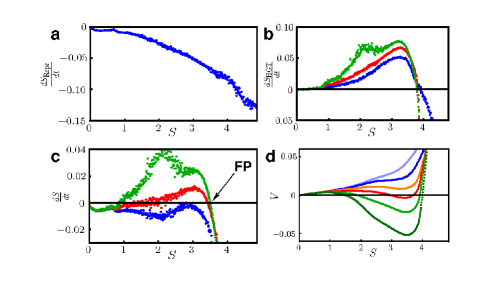
Figure 4: The distributed state disappears for low HGT competence. At a critical competence the dynamical fixed point at high population entropy is destroyed in a saddle-node bifurcation. Here we show the analysis of the system yielding the dynamics illustrated in Figure 2. Panels (a) and (b) show the rate of change of the population entropy due to reproduction and HGT obtained with the methods described in the Methods section. The colors indicate the rate of change for competence values $c=1$ (blue), $c=3$ (red) and $c=5$ (orange). Adding the results from (a) and (b) according to equation (6) yields the overall rate of change $\dot{S}$ for the dynamics shown in (c). The arrow indicates the fixed point at high population entropies emerging through a saddle-node bifurcation for increasing the parameter $c$. With equation (7) we define a potential $V(S)$ for the dynamics which is shown in (d) for the competences $c=1$ (blue), $c=3$ (red) and $c=5$ (orange) and additionally for $c=0.5$ (gray), $c=2$ (green) and $c=4$ (black). The potential valley at high population entropies emerges between $c=1$ and $c=2$ so that the critical competence must lie between these two values. Each dataset was obtained in simulations measuring the dynamics for a time $T=10^{7}$.

Why do the dynamics almost always remain in the high entropy state for high competence? Using the average rate of change $\dot{S}(S)$ we define a potential

$$V(S)=-\int_{0}^{S}\dot{S}(S^{\prime})dS^{\prime}$$ (7)

in which the dynamics move under additional stochastic forcing. This potential is shown in Figure 4d. According to reaction rate theory Hänggi et al. (1990), the depths of the two stable states’ potential wells determine the average time the dynamics stay close to each of the stable states. As the potential well at the distributed state becomes ever deeper for higher competence the dynamics hence stay ever longer in this state.

Thus, our results suggest that when progenotes had high competence for HGT in early evolution, a distributed state was dynamically stable. If competence then decreased below a critical value, the distributed state may have disappeared and triggered the emergence of the first species. For this Darwinian transition to occur, the population’s competence must have decreased dynamically in the distributed state. How could this have happened?

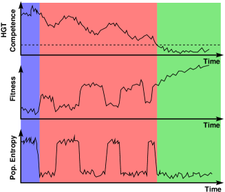
Figure 5: A possible scenario for the evolution of distinct species from a pre-Darwinian distributed state. The three time series sketched here are not simulation data, but encapsulate the speculations in the text, showing how the average competence, the average fitness, and the population entropy may evolve in the transition from a distributed state to the first distinct species. In the initial state (marked in blue) the competence is high, so that HGT drives the dynamics; the population exhibits a high population entropy and low average fitness. Through a stochastic switching the dynamics reaches a state of low population entropy where the fitness is higher as the population adapts to the fitness landscape. Here the population could evolve slowly toward lower competence. Thus, the dynamics switch back and forth between the low and the high entropy state remaining longer and longer in the low entropy state as the competence decreases (marked in red). When the competence goes below a critical value (marked by the dashed line in the top panel) the high entropy state disappears (marked in green), the dynamics remains in the low entropy state, the population’s average fitness increases and the first species may robustly evolve.

A decrease in competence may rely on a mechanism that combines the stochastic switching uncovered above with the suggestion that fitter populations may tend to be less prone to HGT events, as schematically illustrated in Figure 5. As the speciated state is always stable, even if the population’s competence is high, the population dynamics will stochastically switch to this state repeatedly for relatively short times. In the selection-dominated state (i.e., at low $S$) the population’s fitness increases. A fitter population that might be less prone to HGT events, as suggested recently Vogan and Higgs (2011), has a decreased overall competence (lower $c$ in our simplified model setting). Smaller $c$ in turn increases the stochastic residence times the population spends in the selection-dominated state. This combination of two mutually amplifying contributions (decreasing HGT rate and increasing fitness in the population) may yield decreasing competence in the long term such that after sufficiently many switches to the low-$S$ state, the competence may drop below a critical value where the distributed state disappears. The population then stays localized around the fittest genotypes, thus marking the time of transition to Darwinian evolution. At this time, the first species can robustly emerge. The scenario shown schematically in Figure 5 illustrates one potential course of such repeated switching dynamics, with temporarily increased phases of higher fitness and decreasing HGT competence on long time scales.

IV Conclusion

Our results provide a first glimpse of the possible dynamics that may have led to the emergence of the first species from a distributed state dominated by HGT. We demonstrated that a high competence for HGT in a population may suffice to drive the population into a distributed state (Figure 2). In this state HGT dominates the dynamics, in the sense that it inhibits the population’s ability to adapt to the underlying fitness landscape and thus prevents it from crystallizing into distinct species. Our analysis revealed that, independently of the mutation rate exhibited by the population, HGT can drive the population dynamics into a state where the population is widely spread out in genotype space (Figure 3). We identify this state with a pre-Darwinian collective state envisioned by Woese Woese and Fox (1977b); Woese (1998, 2002, 2005).

Similarly, a state where no distinct species exist can emerge if the mutation rate in the population is too large Nowak (2006); Eigen (1971); Eigen and Schuster (1979). Above a critical mutation rate (the error threshold) the population cannot adapt to the underlying fitness landscape and will always evolve toward a quasispecies state Nowak (2006); Eigen (1971); Eigen and Schuster (1979) similar to the distributed state induced by HGT shown above. However, there is a fundamental difference in the dynamics induced by HGT and that induced by mutations: While a mutation rate above an error threshold will always lead to a quasispecies state Nowak (2006), high rates of HGT as studied above induce a bistability of the dynamics where the distributed state coexists with a localized “speciated” state of low $S$. This coexistence may be essential for the evolution toward lower competence in a population and thus for the emergence of the first species; the coexistence is what enables a population originally in a distributed state to repeatedly switch to a low-$S$ state. As selection plays a major role in such a low-$S$ state, progenotes with lower competence would be selected for. Thus, with time, the entire population would evolve toward lower competence until the distributed state disappears as selection effects dominate the dynamics and the first species emerge.

For the breakdown of the distributed state it is essential that the population evolves toward a lower competence. That the latter may in principle be possible was already suggested by Vogan and Higgs Vogan and Higgs (2011). Our results on an idealized model now demonstrate how stochastic switching and fitness-dependent competence may combine to create a transition from a bistable state to a speciated-only state. They in particular also suggest that HGT may be present at similar competence levels before and after the emergence of the first species. From a complementary perspective, whereas one or a few species may already have existed, other population parts may still have been mixed without any clear species. So the very first species may only have marked the beginning of the decline of genuinely non-specific life, with other Darwinian transitions to follow.

Acknowlegdements: We thank Nigel Goldenfeld, Stefan Grosskinsky, Oskar Hallatschek and Arne Traulsen for valuable comments and discussions. Supported by a grant of the Max Planck Society to MT.

References

- Darwin (1859) C. R. Darwin, On the Origin of Species (John Murray, London, UK, 1859).
- Nirenberg et al. (1963) MW Nirenberg, OW Jones, P Leder, BFC Clark, WS Sly, and S Pestka, “On the coding of genetic information,” in Cold Spring Harbor Symposia on Quantitative Biology, Vol. 28 (Cold Spring Harbor Laboratory Press, 1963) pp. 549–557.
- Woese (1967) C. R. Woese, The Genetic Code (Harper and Row, New York, 1967).
- Knight et al. (2001) Robin D Knight, Stephen J Freeland, and Laura F Landweber, “Rewiring the keyboard: evolvability of the genetic code,” Nature Reviews Genetics 2, 49–58 (2001).
- Woese and Fox (1977a) C. R. Woese and G. E. Fox, “Phylogenetic structure of the prokaryotic domain: The primary kingdoms,” Proceedings of the National Academy of Sciences 74, 5088–5090 (1977a).
- Woese (2000) C. R. Woese, “Interpreting the universal phylogenetic tree,” Proc. Natl. Acad. Sci. USA 97, 8392–8396 (2000).
- Ciccarelli et al. (2006) F. D. Ciccarelli, T. Doerks, C. von Mering, C. J. Creevey, B. Snel, and P. Bork, “Toward automatic reconstruction of a highly resolved tree of life,” Science 311, 1283–1287 (2006).
- Pace et al. (2012) N. R. Pace, J. Sapp, and N. Goldenfeld, “Phylogeny and beyond: Scientific, historical, and conceptual significance of the first tree of life,” Proc. Natl. Acad. Sci. USA 109, 1011–1018 (2012).
- Gogarten et al. (1989) J. P. Gogarten, H. Kibak, P. Dittrich, L. Taiz, E. J. Bowman, B. J. Bowman, M. F. Manolsen, R. J. Poole, T. Date, T. Oshima, J. Konishi, K. Denda, and M. Yoshida, “Evolution of the vacuolar H+-atpase: Implications for the origin of Eukaryotes,” Proc. Natl. Acad. Sci. USA 86, 6661–6665 (1989).
- Iwabe et al. (1989) Naoyuki Iwabe, Kei-ichi Kuma, Masami Hasegawa, Syozo Osawa, and Takashi Miyata, “Evolutionary relationship of archaebacteria, eubacteria, and eukaryotes inferred from phylogenetic trees of duplicated genes,” Proceedings of the National Academy of Sciences 86, 9355–9359 (1989).
- Theobald (2010) D. L. Theobald, “A formal test of the theory of universal common ancestry,” Nature 415, 219–223 (2010).
- Dagan et al. (2010) Tal Dagan, Mayo Roettger, David Bryant, and William Martin, “Genome networks root the tree of life between prokaryotic domains,” Genome Biology and Evolution 2, 379–392 (2010).
- Williams et al. (2013) Tom A Williams, Peter G Foster, Cymon J Cox, and T Martin Embley, “An archaeal origin of eukaryotes supports only two primary domains of life,” Nature 504, 231–236 (2013).
- Glansdorff et al. (2008) Nicolas Glansdorff, Ying Xu, Bernard Labedan, et al., “The last universal common ancestor: emergence, constitution and genetic legacy of an elusive forerunner,” Biol Direct 3, 56–125 (2008).
- Woese and Fox (1977b) C. R. Woese and G. E. Fox, “The concept of cellular evolution,” J. Mol. Evol. 10, 1–6 (1977b).
- Woese (1998) C. R. Woese, “The universal ancestor,” Proc. Natl. Acad. Sci. USA 95, 6854–6859 (1998).
- Woese (2002) C. R. Woese, “On the evolution of cells,” Proc. Natl. Acad. Sci. USA 99, 8742–8747 (2002).
- Woese (2005) C. R. Woese, “Evolving biological organization,” in Microbial Phylogeny and Evolution: Concepts and Controversies, edited by J. Sapp (Oxford University Press, Oxford, UK, 2005) pp. 99–117.
- Vetsigian et al. (2006) K. Vetsigian, C.Woese, and N. Goldenfeld, “Collective evolution and the genetic code,” Proc. Natl. Acad. Sci. USA 103, 10696–10701 (2006).
- Haig and Hurst (1991) David Haig and Laurence D Hurst, “A quantitative measure of error minimization in the genetic code,” Journal of Molecular Evolution 33, 412–417 (1991).
- Freeland and Hurst (1998) Stephen J Freeland and Laurence D Hurst, “The genetic code is one in a million,” Journal of Molecular Evolution 47, 238–248 (1998).
- Butler et al. (2009) Thomas Butler, Nigel Goldenfeld, Damien Mathew, and Zaida Luthey-Schulten, “Extreme genetic code optimality from a molecular dynamics calculation of amino acid polar requirement,” Physical Review E 79, 060901 (2009).
- Drossel (2001) B. Drossel, “Biological evolution and statistical physics,” Adv. Phys. 50, 209–295 (2001).
- Syvanen (1985) M. Syvanen, “Cross-species gene transfer; implications for a new theory of evolution,” J. Theor. Biol. 112, 333–343 (1985).
- Syvanen (1994) M. Syvanen, “Horizontal gene transfer: Evidence and possible consequences,” Annu. Rev. Genet. 28, 237–261 (1994).
- Delsuc et al. (2005) F. Delsuc, H. Brinkmann, and H. Philippe, “Phylogenomics and the reconstruction of the tree of life,” Nat. Rev. Genet. 6, 361–375 (2005).
- Thomas and Nielsen (2005) C. M. Thomas and K. M. Nielsen, “Mechanisms of, and barriers to, horizontal gene transfer between bacteria,” Nat. Rev. Microbiol. 3, 711–721 (2005).
- Anderson (1966) ES Anderson, “Possible importance of transfer factors in bacterial evolution,” Nature 209, 637–638 (1966).
- Anderson (1970) Norman G Anderson, “Evolutionary significance of virus infection,” Nature 227, 1346–1347 (1970).
- Sonea (1988) Sorin Sonea, “A bacterial way of life,” Nature 331, 216 (1988).
- Kurland et al. (2003) C. G. Kurland, B. Canback, and O. G. Berg, “Horizontal gene transfer: A critical view,” Proc. Natl. Acad. Sci. U. S. A. 100, 9658–9662 (2003).
- Dagan and Martin (2006) T. Dagan and W. Martin, “The tree of one percent,” Genome Biol. 7, 118 (2006).
- Takeuchi et al. (2014) Nobuto Takeuchi, Kunihiko Kaneko, and Eugene V Koonin, “Horizontal gene transfer can rescue prokaryotes from mullerÕs ratchet: Benefit of dna from dead cells and population subdivision,” G3: Genes | Genomes | Genetics 4, 325–339 (2014).
- Cohan (2002) Frederick M Cohan, “What are bacterial species?” Annual Reviews in Microbiology 56, 457–487 (2002).
- Lawrence (2002) Jeffrey G Lawrence, “Gene transfer in bacteria: speciation without species?” Theoretical Population Biology 61, 449–460 (2002).
- Gevers et al. (2005) Dirk Gevers, Frederick M Cohan, Jeffrey G Lawrence, Brian G Spratt, Tom Coenye, Edward J Feil, Erko Stackebrandt, Yves Van de Peer, Peter Vandamme, Fabiano L Thompson, et al., “Re-evaluating prokaryotic species,” Nature Reviews Microbiology 3, 733–739 (2005).
- Konstantinidis and Tiedje (2005) Konstantinos T Konstantinidis and James M Tiedje, “Genomic insights that advance the species definition for prokaryotes,” Proceedings of the National Academy of Sciences USA 102, 2567–2572 (2005).
- Staley (2006) James T Staley, “The bacterial species dilemma and the genomic–phylogenetic species concept,” Philosophical Transactions of the Royal Society B: Biological Sciences 361, 1899–1909 (2006).
- Zhaxybayeva and Doolittle (2011) O. Zhaxybayeva and W. F. Doolittle, “Lateral gene transfer,” Curr. Biol. 21, R242–R246 (2011).
- Goldenfeld and Woese (2007) N. Goldenfeld and C. Woese, “Biology’s next revolution,” Nature 445, 369 (2007).
- Dyson (2007) F. Dyson, “Our biotech future,” New York Review of Books July 19 (2007).
- Taylor et al. (2004) C. Taylor, D. Fudenberg, A. Sasaki, and M. A. Nowak, “Evolutionary game theory in finite populations,” Bull. Math. Biol. 66, 1621–1644 (2004).
- Traulsen et al. (2005) A. Traulsen, J. C. Claussen, and C. Hauert, “Coevolutionary dynamics: From finite to infinite populations,” Phys. Rev. Lett. 95, 238701 (2005).
- Nowak (2006) M. A. Nowak, Evolutionary Dynamics (Harvard University Press, London, UK, 2006).
- Durrett and Schmidt (2008) R. Durrett and D. Schmidt, “Waiting for two mutations: With applications to regulatory sequence evolution and the limits of Darwinian evolution,” Genetics 180, 1501–1509 (2008).
- Arnoldt et al. (2012) H. Arnoldt, M. Timme, and S. Grosskinsky, “Frequency dependent fitness induces multistability in coevolutionary dynamics,” J. R. Soc. Interface 9, 3387–3396 (2012).
- Leisner et al. (2008) M. Leisner, K. Stingl, E. Frey, and B. Maier, “Stochastic switching to competence,” Curr. Opin. Microbiol. 11, 553–559 (2008).
- Moran and Jarvik (2010) N. A. Moran and T. Jarvik, “Lateral transfer of genes from fungi underlies carotenoid production in aphids,” Science 328, 624–627 (2010).
- Mayer et al. (2011) W. E. Mayer, L. N. Schuster, G. Bartelmes, C. Dieterich, and R. J. Sommer, “Horizontal gene transfer of microbial cellulases into nematode genomes is associated with functional assimilation and gene turnover,” BMC Evol. Biol. 11, 13 (2011).
- Vogan and Higgs (2011) A. A. Vogan and P. G. Higgs, “The advantages and disadvantages of horizontal gene transfer and the emergence of the first species,” Biol. Direct 6, 1 (2011).
- Fuentes et al. (2014) I. Fuentes, S. Stegemann, H. Golczyk, D. Karcher, and R. Bock, “Horizontal genome transfer as an asexual path to the formation of new species,” Nature (2014).
- Wylie et al. (2010) C. S. Wylie, A. D. Trout, D. A. Kessler, and H. Levine, “Optimal strategy for competence differentiation in bacteria,” PLoS Genetics 6 (2010), doi: 10.1371/journal.pgen.1001108.
- Wilke et al. (2001) C. O. Wilke, C. Ronnewinkel, and T. Martinez, “Dynamic fitness landscapes in molecular evolution,” Phys. Rep. 349, 395–446 (2001).
- Moran (1962) P. A. P. Moran, The Statistical Processes of Evolutionary Theory (Clarendon Press, Oxford, UK, 1962).
- Leisner et al. (2009) M. Leisner, J.-T. Kuhr, J. O. Rädler, E. Frey, and B. Maier, “Kinetics of genetic switching into the state of bacterial competence,” Biophys. J. 96, 1178–1188 (2009).
- Kovacs et al. (2009) A. T. Kovacs, W. K. Smits, A. M. Mironczuk, and O. P. Kuipers, “Ubiquitous late competence genes in bacillus species indicate the presence of functional dna uptake machineries,” Environ. Microbiol. 11, 1911–1922 (2009).
- Hänggi et al. (1990) P. Hänggi, P. Talkner, and M. Borkovec, “Reaction rate theory: Fifty years after Kramers,” Rev. Mod. Phys. 62, 251–342 (1990).
- Eigen (1971) M. Eigen, “Selforganization of matter and the evolution of biological macromolecules,” Die Naturwissenschaften 58, 465–523 (1971).
- Eigen and Schuster (1979) M. Eigen and P. Schuster, The Hypercycle: A Principle of Natural Self-Organization (Springer-Verlag, Berlin, Germany, 1979).