Determination of the stretch tensor for structural transformations

Abstract

The transformation stretch tensor plays an essential role in the evaluation of conditions of compatibility between phases and the use of the Cauchy-Born rule. This tensor is difficult to measure directly from experiment. We give an algorithm for the determination of the transformation stretch tensor from x-ray measurements of structure and lattice parameters. When evaluated on some traditional and emerging phase transformations the algorithm gives unexpected results.

The structural transformations commonly occur in application of functional materials. Typical examples of phase transformation driven phenomena include shape memory alloys, ferroelectricity, piezoelectricity, colossal magnetoresistance and superconductivity. It has been demonstrated that material reliability depends, essentially, on the reversibility of the transformation. It is therefore important to understand how reversibility can be achieved and how the transformation occurs at the lattice and atomic level. The transformation stretch tensor, $\mathbf{U}$, is the stretch part of the linear transformation that maps the crystal structure from its initial phase to the final phase Ball and James (1987, 1992); Bhattacharya (2003); Chen et al. (2011). Recently, the reversibility, the thermal hysteresis, and the resistance to cyclic degradation of functional materials have been linked to properties of the transformation stretch tensor. For example, when the middle eigenvalue $\lambda_{2}$ of $\mathbf{U}$ is tuned to the value 1 by compositional changes, the measured width of the thermal hysteresis loop drops precipitously to near 0 in diverse alloy systems Cui et al. (2006); Zarnetta et al. (2010); Chen et al. (2013). Assuming the Cauchy-Born rule for martensitic materials Bhattacharya (2003); Ericksen (2008); Pitteri and Zanzotto (2010), the condition $\lambda_{2}=1$ implies a special condition of compatibility between phases by which the undistorted austenite phase and a single undistorted variant of the martensite phase fit perfectly together at an interface. Even stronger conditions of compatibility known as the cofactor conditions ($\lambda_{2}=1$ together with either $|\mathbf{U}^{-1}\mathbf{e}|=1$ or $|\mathbf{U}\mathbf{e}|=1$, where $\mathbf{e}$ is unit vector on a 2-fold symmetry axis of austenite), lead to even lower hysteresis and significantly enhanced reversibility during cyclic transformation Song et al. (2013). $\mathbf{U}$ also plays an important role in determining the elastically favored orientations of precipitates for diffusional transformations Voorhees, P. W. and Johnson, W. C (1988); Chen et al. (2011).

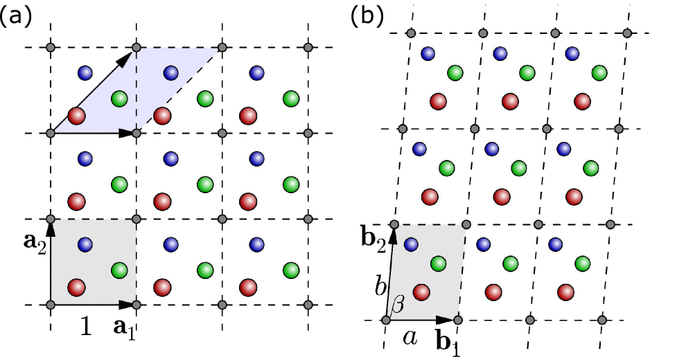
Figure 1: Non-uniqueness of Cauchy-Born deformation gradient from (a) square lattice to (b) oblique lattice. Red, blue and green balls represent different atomic species. Gray dots are lattice points

In principle, the determination of the stretch tensor $\mathbf{U}$ for a structural transformation is straightforward. Suppose the primitive lattice vectors of initial and final phases are, respectively, linearly independent vectors $\mathbf{a}_{i}$ and $\mathbf{b}_{i}$ for $i=1,2,...d$ where $d$ is the dimension of the lattice. A nonsingular linear transformation $\mathbf{F}$ can be defined uniquely by

$$\mathbf{F}\mathbf{a}_{i}=\mathbf{b}_{i},\quad i=1,2,...d,$$ (1)

and the polar decomposition of $\mathbf{F}$ is written $\mathbf{F}=\mathbf{Q}\mathbf{U}$, where $\mathbf{Q}$ is orthogonal and $\mathbf{U}$ is positive-definite and symmetric, called the transformation stretch tensor. The notation $\mathbf{a}_{i}\to\mathbf{b}_{i}$ denotes the lattice correspondence. In the case of transformation in Fig. 1, one choice of the lattice correspondence can be $\mathbf{a}_{1}\to\mathbf{b}_{1},\ \mathbf{a}_{2}\to\mathbf{b}_{2}$ where $\mathbf{a}_{1}=[1,0]$, $\mathbf{a}_{2}=[0,1]$ and $\mathbf{b}_{1}=[a,0]$ and $\mathbf{b}_{2}=[b\cos\beta,b\sin\beta]$.

As is well-known Wayman (1964); Bowles and Wayman (1972), $\mathbf{F}$ and $\mathbf{U}$ are not uniquely determined by the two lattices. This follows from the fact that there are infinitely many choices of lattice correspondence. From Fig. 1, the alternative set of vectors $\mathbf{a}_{1}$ and $\mathbf{a}_{1}+\mathbf{a}_{2}$ describes the same lattice (a), which results in a different correspondence from (a) to (b). This obviously changes the $\mathbf{F}$ and thus the transformation stretch tensor $\mathbf{U}$. More generally, any two sets of primitive lattice vectors for a given lattice are related by a lattice invariant transformation Ball and James (1992) i.e., a unimodular matrix of integers. If we allow an invariant transformation for both initial and final phases, the ambiguity of $\mathbf{F}$ is $\mathbf{F}\to\Lambda_{\text{(f)}}\mathbf{F}\Lambda_{\text{(i)}}^{-1}$ where $\Lambda_{\text{(i)}}$ and $\Lambda_{\text{(f)}}$ denote the lattice invariant transformation for initial and final lattices, respectively.

The linear transformation $\mathbf{F}$ represents the change of periodicity of the two phases. The individual atoms denoted by the red, blue and green balls in Fig. 1 may shuffle in various ways, giving rise to different space group symmetries, but it is the linear transformation $\mathbf{F}$ that relates to macroscopic deformation and therefore to conditions of compatibility (Bowles and Mackenzie, 1954; Lieberman et al., 1957; Wayman, 1964; Knowles and Smith, 1981; Ericksen, 1984; Ball and James, 1987; Ericksen, 2008; Pitteri and Zanzotto, 2010; Zhang et al., 2009; Chen et al., 2013). This idea is formalized by the weak Cauchy-Born rule Ericksen (2008); Bhattacharya et al. (2004). This rule is used to define the dependence on deformation of the free energy at continuum scale from the free energy density at atomistic scale for complex lattices with multiple atoms per unit cell and inhomogeneous deformations. Inhomogeneous deformations $\mathbf{y}(\mathbf{x})$ locally satisfy the same rule as above: $\mathbf{b}_{i}=\nabla\mathbf{y}\,\mathbf{a}_{i}$, where $\mathbf{a}_{i}$ and $\mathbf{b}_{i}$ represent the local periodicity. Note that we use a geometrically exact description here. A geometrically linear description (i.e., as in linear elasticity) would not be sufficiently accurate to describe transformations here for the purposes of imposing the conditions of compatibility (see Chen et al. (2013) for calculations of the error in various cases).

Based on a natural intuition that “a mode of atomic shift requires minimum motion” (Bain and Dunkirk, 1924), Bain proposed a famous lattice correspondence in 1924 for the formation of bcc $\alpha$Fe from fcc $\gamma$Fe . The correspondence has been well-accepted and applied to study numerous phase transformations Tadaki and Shimizu (1970); Otsuka et al. (1971); Knowles and Smith (1980); Chu (193); Ball and James (1992); Bhattacharya (2003); Huang et al. (2003). To illustrate how easy the Bain correspondence misses the smallest strain, we construct an example of transformation from a bcc lattice with $a_{0}=1$ to a monoclinic lattice with $a=0.961$, $b=1.363$, $c=1.541$, and $\beta=97.78^{\circ}$. Fig. 2(a) shows the bcc lattice with two sublattice unit cells (red and blue). Conventional wisdom would say that the Bain correspondence (red $\to$ gray in Fig. 2(b), bottom) is appropriate for this transformation. However, our algorithm proposed later in this letter reveals an unexpected alternative correspondence (blue $\to$ gray, Fig. 2 (b), top). Both contain 4 lattice points ($n=4$) in the unit cells, and the shape and size of them are similar to the primitive cell of monoclinic lattice. Fig. 2(b) shows the comparison of distortions for both transformation mechanisms. Notice that both mechanisms give exactly the same final monoclinic lattice. However, by quantitative calculation, the principle strains for the new correspondence are in fact smaller than those for the Bain correspondence.

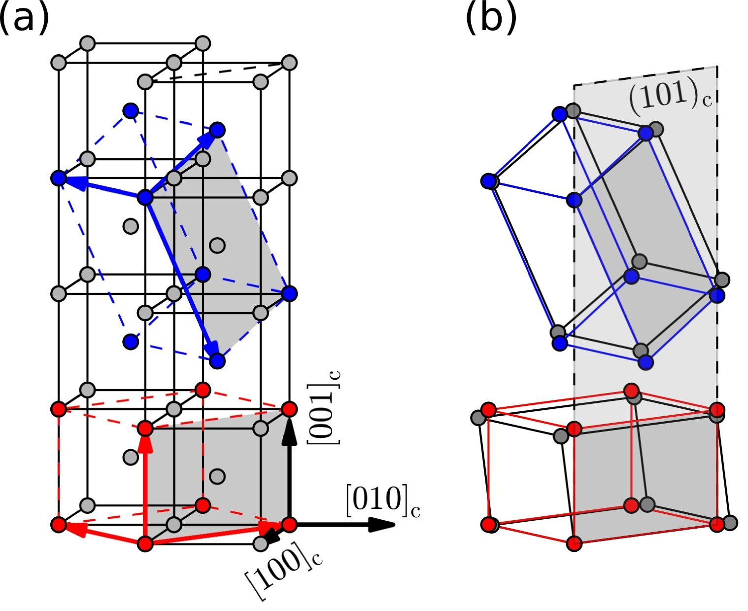
Figure 2: The least atomic movements during the structural transformation. (a) The bcc lattice and two of its sublattices (red and blue) of size 4. (b) Comparison between these bcc sublattice unit cells and the primitive cell of the final phase (gray; for clarity atoms in the unit cell are not shown).

The significance of finding the correct lattice correspondence for structural phase transformations is emphasized in the literature Wayman (1964); Bowles and Wayman (1972). The problem was well-appreciated by Lomer Lomer (1955) as early as the mid-1950s. In his study of the mechanism of the $\beta\to\alpha$ phase transformation of U_98.6Cr_1.4, he examined theoretically (by hand) 1,600 possible transformation mechanisms, and reduced this to three correspondences having the smallest principle strains, which he considered the likely candidates.

Direct experimental measurement of the macroscopic finite strain of transformation, together with accurate structural characterization by X-ray diffraction provides a possible way to determine the lattice correspondence and thus the transformation stretch tensor. But this is technically difficult due to (i) the need for an oriented single crystal, (ii) the need to remove the inevitable fine microstructures that form during transformation due to constraints of compatibility, and (iii) the need for an accurate measure of full finite strain tensor along known crystallographic directions. We also noticed that using a state-of-art high resolution TEM on a pre-oriented single crystal sample can not definitively remove the ambiguities among many lattice correspondences due to some inevitable obstacles: tracking the evolution of diffraction spots in a fast structural transformation process, simultaneously indexing both phases, and most significantly, finding a special zone that can unambiguously reveal the differences among various lattice correspondences.

In this letter we propose an algorithmic approach to search the $N$ best choices of lattice correspondence for a structural transformation, by minimizing a particular strain measure between initial and final lattices. The input to the algorithm is the underlying periodicities (the remaining space group information is not needed) and the lattice constants of the two phases. The output from the algorithm is the $N$ best choices of lattice correspondence and the associated transformation stretch tensors. Users can customize how many solutions they like by manipulating $N$. The results can be used as a reference by the advanced structural characterization facilities for the determination of orientation relationships, and it can be integrated with first principles calculations to give starting points for the determination of energy barriers or interfacial distortion profiles.

Consider a Bravais lattice ${\cal L}=\{\sum n^{i}\mathbf{e}_{i}:n^{1},\dots n^{d}\in\mathbb{Z}^{d}\}$ determined by linearly independent lattice vectors $\mathbf{e}_{1},\dots,\mathbf{e}_{d}\in\mathbb{R}^{d}$, $i=1,\ldots,d$, and assemble the lattice vectors as the columns of a $d\times d$ matrix $\mathbf{E}=(\mathbf{e}_{1},\ldots,\mathbf{e}_{d})$. $\cal L$ can equivalently be denoted

$${\cal L}={\cal L}(\mathbf{E})=\big{\{}\mathbf{r}\in\mathbb{R}^{d}:\mathbf{r}=\mathbf{E}\mathbf{\bm{\xi}},\mathbf{\bm{\xi}}\in\mathbb{Z}^{d}\big{\}}.$$

Without loss of generality, by switching the sign of $\mathbf{e}_{1}$ if necessary, we assume that $\det\mathbf{E}>0$. This determinant is the ($d$-dimensional) volume of a unit cell of ${\cal L}(\mathbf{E})$.

Given two lattices ${\cal L}(\mathbf{E})$ and ${\cal L}(\mathbf{E}^{\prime})$, the $d\times d$ nonsingular matrix $\mathbf{L}$ satisfying $\mathbf{E}^{\prime}=\mathbf{E}\mathbf{L}$ is called the correspondence matrix from ${\cal L}(\mathbf{E})$ to ${\cal L}(\mathbf{E}^{\prime})$. As noted above, the two lattices ${\cal L}(\mathbf{E})$ and ${\cal L}(\mathbf{E}^{\prime})$ are the same if and only if the correspondence matrix $\mathbf{L}$ is a unimodular matrix of integers, or, briefly, $\mathbf{L}\in GL(d,\mathbb{Z})$. If a correspondence matrix $\mathbf{L}$ is a matrix of integers with $|\det\mathbf{L}|>1$, then ${\cal L}(\mathbf{E}^{\prime})$ is a sublattice of ${\cal L}(\mathbf{E})$. The quantity $|\det\mathbf{L}|$ is the volume ratio of the unit cell of $\mathcal{L}(\mathbf{E}^{\prime})$ to that of $\mathcal{L}(\mathbf{E})$.

Correspondence matrices are often reported for conventional rather than primitive descriptions, particularly for 7 of the 14 types of Bravais lattices in 3D. For example, the conventional description for an fcc lattice with lattice parameter $a_{0}$ is an orthogonal basis, so $\mathbf{E}_{\rm conv}=a_{0}\mathbf{I}=\mathbf{E}\mathbf{\bm{\chi}}$, where, for example,

$$\mathbf{E}=\frac{a_{0}}{2}\begin{bmatrix}1&0&1\\ 1&1&0\\ 0&1&1\end{bmatrix},~{}~{}\mathbf{\bm{\chi}}=\begin{bmatrix}1&1&-1\\ -1&1&1\\ 1&-1&1\end{bmatrix}.$$

Here, $\det\mathbf{\bm{\chi}}=4$ so the volume of the conventional unit cell is 4 times that of the primitive cell. From now on, the symbol $\mathbf{\bm{\chi}}$ is reserved for a correspondence matrix from the primitive to conventional unit cell of a Bravais lattice: $\mathbf{E}_{\rm conv}=\mathbf{E}\mathbf{\bm{\chi}}$.

We seek a sublattice of $\mathcal{L}(\mathbf{E}_{A})$ that is mapped to the primitive lattice of $\mathcal{L}(\mathbf{E}_{B})$. (The algorithm can easily handle the case in which we take sublattices of both lattices.) As above, let $\mathbf{E}_{A}=(\mathbf{a}_{1},...,\mathbf{a}_{d})$ and $\mathbf{E}_{B}=(\mathbf{b}_{1},...,\mathbf{b}_{d})$. Let $\mathbf{\bm{\ell}}\in\mathbb{Z}^{d\times d}$, $\det\mathbf{\bm{\ell}}>0$, be the correspondence matrix giving the sublattice $\mathcal{L}(\mathbf{E}_{A}\mathbf{\bm{\ell}})$ that is mapped to the final lattice $\mathcal{L}(\mathbf{E}_{B})$ during the transformation. The basic equation (1) in this case becomes $\mathbf{F}\mathbf{E}_{A}\mathbf{\bm{\ell}}=\mathbf{E}_{B}$, and the transformation stretch tensor $\mathbf{U}$ is the unique positive-definite square root of $\mathbf{F}^{T}\mathbf{F}$.

We introduce the following function as a measure of the distance from $\mathbf{U}$ to $\mathbf{I}$:

$$\begin{split}\text{dist}(\mathbf{\bm{\ell}},\mathbf{\bm{E}}_{A},\mathbf{\bm{E}}_{B})&=\left\|(\mathbf{F}^{T}\mathbf{F})^{-1}-\mathbf{I}\right\|^{2}\\ &=\left\|\mathbf{\bm{E}}_{A}\mathbf{\bm{\ell}}\mathbf{\bm{E}}_{B}^{-1}\mathbf{\bm{E}}_{B}^{-T}\mathbf{\bm{\ell}}^{T}\mathbf{\bm{E}}_{A}^{T}-\mathbf{\bm{I}}\right\|^{2}.\end{split}$$ (2)

$\|\cdot\|$ denotes the Euclidean norm, $\|\mathbf{\bm{A}}\|=\sqrt{\text{tr\,}\mathbf{\bm{A}}^{T}\mathbf{\bm{A}}}$. The distance (2) is independent of rigid rotations of both lattices, and is particularly attractive from the point of view of symmetry. Physically, it represents the Lagrangian strain of the structural transformation. The use of inverse of $\mathbf{F}^{T}\mathbf{F}$ avoids possible noninvertibility of $\mathbf{\bm{\ell}}$ that may arise during the minimization process. In addition, this norm is exactly preserved by point group transformations of both Bravais lattices. That is, if orthogonal tensors $\mathbf{\bm{R}}_{A}$ and $\mathbf{\bm{R}}_{B}$ are, respectively, in the point groups of $\mathcal{L}(\mathbf{E}_{A})$ and $\mathcal{L}(\mathbf{E}_{B})$, i.e., $\mathcal{L}(\mathbf{E}_{A})=\mathcal{L}(\mathbf{R}_{A}\mathbf{E}_{A})$ and $\mathcal{L}(\mathbf{E}_{B})=\mathcal{L}(\mathbf{R}_{B}\mathbf{E}_{B})$, which, by the above implies that there exist associated matrices $\mathbf{\bm{\mu}}_{A}$ and $\mathbf{\bm{\mu}}_{B}$ such that $\mathbf{R}_{A}\mathbf{E}_{A}=\mathbf{E}_{A}\mathbf{\bm{\mu}}_{A}$ and $\mathbf{R}_{B}\mathbf{E}_{B}=\mathbf{E}_{B}\mathbf{\bm{\mu}}_{B}$ then the distance transforms as

$$\text{dist}(\mathbf{\bm{\mu}}_{A}\mathbf{\bm{\ell}}\mathbf{\bm{\mu}}_{B},\mathbf{\bm{E}}_{A},\mathbf{\bm{E}}_{B})=\text{dist}(\mathbf{\bm{\ell}},\mathbf{\bm{E}}_{A},\mathbf{\bm{E}}_{B}).$$ (3)

Note that $\mathbf{\bm{\mu}}_{A,B}$ are integral matrices of determinant $\pm 1$, so $\det\mathbf{\bm{\ell}}=\det\mathbf{\bm{\mu}}_{A}\mathbf{\bm{\ell}}\mathbf{\bm{\mu}}_{B}$. Thus, immediately one minimizer of the distance with assigned determinant gives the expected symmetry-related minimizers. Physically, in the typical case of a symmetry-lowering transformation, e.g. the martensitic transformation, the distance function (2) automatically gives the equi-minimizing variants of martensite.

As noted above it is typical to report the correspondence matrix in terms of the conventional basis instead of the primitive one. If $\mathbf{\bm{\ell}}^{*}$ is a minimizer of $\text{dist}(\mathbf{\bm{\ell}},\mathbf{\bm{E}}_{A},\mathbf{\bm{E}}_{B})$ the conversion is done by $\mathbf{L}^{*}=\mathbf{\bm{\chi}}_{A}^{-1}\mathbf{\bm{\ell}}^{*}\mathbf{\bm{\chi}}_{B}$. Note that $\mathbf{L}^{*}$ is not necessarily a matrix of integers.

A significant property of the distance function (2) will be used to justify our algorithm below. Fixing $\mathbf{E}_{A}$ and $\mathbf{E}_{B}$, the distance function can be trivially extended to a function over real matrices, $f(\mathbf{L})={\rm dist}(\mathbf{L},\mathbf{E}_{A},\mathbf{E}_{B})$. Denoting $\mathbf{X}_{L}=\mathbf{E}_{A}\mathbf{L}\mathbf{E}_{B}^{-1}\mathbf{\bm{E}}_{B}^{-T}\mathbf{L}^{T}\mathbf{\bm{E}}_{A}^{T}$ and using $\mathbf{X}_{L}\cdot\mathbf{I}\leq\left\|\mathbf{X}_{L}\right\|\left\|\mathbf{I}\right\|=\sqrt{3}\left\|\mathbf{X}_{L}\right\|$, we have

$$\begin{split}f(\mathbf{L})&=\left\|\mathbf{X}_{L}\right\|^{2}-2\mathbf{X}_{L}\cdot\mathbf{\bm{I}}+3\\ &\geqslant\left\|\mathbf{X}_{L}\right\|^{2}-2\sqrt{3}\left\|\mathbf{X}_{L}\right\|+3=(\left\|\mathbf{X}_{L}\right\|-\sqrt{3})^{2},\end{split}$$ (4)

Choose any integral matrix $\mathbf{\bm{\ell}}_{1}$ and define $C_{1}=f(\mathbf{\bm{\ell}}_{1})$. By (4) the minimizer(s) of $f(\mathbf{L})$ necessarily lie in the bounded set $\left\|\mathbf{X}_{L}\right\|\leq\sqrt{3}+\sqrt{C_{1}}$, that is, $\left\|\mathbf{X}_{L}\right\|^{2}\leq 3+C_{1}+2\sqrt{3C_{1}}.$ Let $\alpha$ be the minimum of $\|\mathbf{X}_{L}\|^{2}$ under the constraint $\|\mathbf{L}\|=1$, then we have

$$\alpha\|\mathbf{L}\|^{4}\leqslant\left\|\mathbf{X}_{L}\right\|^{2}<3+C_{1}+2\sqrt{3C_{1}}.$$ (5)

That is, all the $\mathbf{L}$’s such that $f(\mathbf{L})<C$ live in the sphere with the radius of $((3+C_{1}+2\sqrt{3C_{1}})/\alpha)^{1/4}$ in $\mathbb{R}^{9}$.

Here is a brief outline of the algorithm for the determination of the $N$ best transformation stretch tensors and their associated lattice correspondences:

1. Calculate the primitive bases and the transformation matrices for the conventional cells from the input lattice parameters: $\mathbf{E}_{\text{A, B}}$ and $\mathbf{\bm{\chi}}_{\text{A, B}}$. Calculate $\alpha$ by minimizing the term $\mathbf{X}_{L}$ with respect to $\mathbf{L}$ for all $\|\mathbf{L}\|=1$.

2. Choose $N$ integral matrices ${\mathbf{\bm{\ell}}_{i}}$, $i=1,\ldots,N$ as the initial guess of the solution list such that $\det\,\mathbf{\bm{\ell}}_{i}$ is close to $\det\mathbf{E}_{B}/\det\mathbf{E}_{A}$ and ${\rm dist}(\mathbf{\bm{\ell}}_{i},\mathbf{E}_{A},\mathbf{E}_{B})$ is small.

3. Let $C_{1}$ be the maximum $f(\mathbf{\bm{\ell}}_{i})$ for $\mathbf{\bm{\ell}}_{i}$’s in the solution list.

4. Calculate the distance for all integral matrices in the sphere of radius of $((3+C_{1}+2\sqrt{3C_{1}})/\alpha)^{1/4}$. Update the solution list as necessary. If the solution list is changed, repeat from step 3.

5. For each solution $\mathbf{\bm{\ell}}_{i}$, calculate the Cauchy-Born deformation gradient $\mathbf{F}_{i}=\mathbf{E}_{B}(\mathbf{E}_{A}\mathbf{\bm{\ell}}_{i})^{-1}$ and the transformation stretch tensor $\mathbf{U}_{i}=(\mathbf{F}_{i}^{T}\mathbf{F}_{i})^{1/2}$. Finally, rewrite all the solutions in the conventional bases: $\mathbf{L}^{*}_{i}=\mathbf{\bm{\chi}}_{\text{A}}^{-1}\mathbf{\bm{\ell}}_{i}\mathbf{\bm{\chi}}_{\text{B}}$.

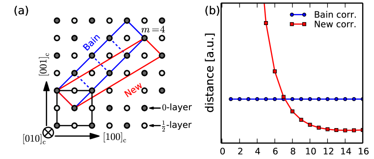
Figure 3: Two possible lattice correspondences in an FCC to monoclinic transformation. (a) (010) projection of the FCC lattice: the dark (resp. light) atoms are in the $y=0$ (resp. $y=1/2$) planes. The solid blue and red lines represent the two lattice correspondences respectively for $m=4$, where the the Bain correspondence is in blue. The dashed blue lines indicate the modulation numbers $m=1,2,3,4$. (b) shows the dependence of the values of the distance function on the modulation of the monoclinic $c$-axis for the two lattice correspondences.

Note that the algorithm converges in a finite number of steps and gets all matrices with the $N$ lowest distances (up to the degeneracy in (3)) because it searches through all matrices of integers satisfying the rigorous bounds (5).

In Fig. 3 we give an example computed by the algorithm that reveals a switch from Bain correspondence to a new correspondence with increasing lattice complexity. Consider a transformation from an fcc lattice with lattice parameter $a_{0}=2$ to a monoclinic lattice with lattice parameters $a=1.41,\ b=1.99,\ c=1.42\,m,\ \beta=86^{\circ}$, where the integer $m>0$ denotes the modulation along monoclinic $c$-axis. Fig. 3(a) shows the undeformed fcc lattice projected onto $(010)$ plane. The two correspondences given by the algorithm are depicted for the $m=4$ case. Fig. 3(b) shows the change in distance function for the two correspondences with $m$ varying from 1 to 16. Initially Bain correspondence is much smaller than the new one, however it loses its privilege after the $7$th modulation. The results suggest that both kinds of lattice correspondence can be feasible in a structural transformation for some special lattice parameters, and in this case $m=7$ has this special status. As mentioned above, these long stacking period structures are common in martensitic phase transformations.

Table 1 shows the results calculated by the algorithm for six materials. The types of transformation are diverse and the principle stretches are consistent with the references. Among these examples, we list two solutions for Zn₄₅Au₃₀Cu₂₅. The material has been recently found to satisfy the cofactor conditions (the 2 constraints on $\mathbf{U}$ explained in paragraph 1) Chen et al. (2013), which have been shown Song et al. (2013) to promote unusually low thermal hysteresis ($\approx 2^{\circ}$C) and enhanced reversibility, owing to a fluid-like flexible martensite microstructure. It was believed Song et al. (2013) to transform by the second solution, Table 1. However, the first solution is the one having the smallest transformation strain. Coincidentally, the new transformation stretch tensor also satisfies closely the cofactor conditions. To investigate this further, the same sample of Zn₄₅Au₃₀Cu₂₅ used in Song et al. (2013) was characterized by synchrotron X-ray Laue microdiffraction. The experiment has been conducted on beamline 12.3.2 of the Advanced Light Source, Lawrence Berkeley National Laboratory. Details on the experimental setup can be found in Kunz et al. (2009). The Laue patterns were collected continuously as heating/cooling through the transformation temperature. These patterns were analyzed and indexed using the XMAS software Tamura (2014). The orientation relationships are determined as the closest parallelisms of the crystallographic planes and zone axes between the indexed Laue patterns of austenite and martensite respectively. They are $(206)_{\text{a}}||(20\,\bar{34})_{\text{m}}$, $(204)_{\text{a}}||(10\,\bar{26})_{\text{m}}$, $[21\bar{1}]_{\text{a}}||[26\,\bar{9}\,1]_{\text{m}}$, $[010]_{\text{a}}||[010]_{\text{m}}$ and $[1\bar{1}0]_{\text{a}}||[8\bar{9}1]_{\text{m}}$ (see supplementary for indexed diffraction patterns). However, this determination with accepted error bars does not definitively distinguish these two mechanisms, since these relationships are so close that one could imagine that both mechanisms occur simultaneously in the material.

In addition to the reversible martensitic transformation, the algorithm is applicable to a wide range of phase transformations even if the initial and final crystal structures do not have a group/sub-group relation. Examples are Ti₉₅Mn₅ and Sb₂Te₃/PbTe (Table 1). The algorithm can be also applied to organic materials when the molecular chains have sufficient periodicity. One extreme example is the polymorphic transformation between two triclinic lattices in terephthalic acid (see Table 1). In this case the calculated principle stretches agree well with the measured macroscopic deformation of the polymorphic transformation of this material.

Table 1: Transformation principle stretches (p. s.), the associated lattice correspondences (lat. cor.) and derived orientation relationships (o. r.) for various phase-transforming materials

materials	p. s.	lat. cor.	derived o. r.
Zn45Au30Cu25 Song et al. (2013) ${\rm L}2_{1}\to{\rm M18R}$	$0.9363$	$[\frac{1}{2}0\frac{1}{2}]_{\text{L2}_{1}}\to[100]_{\text{M}}$	$(204)_{\text{L2}_{1}}||(\bar{1}\,0\,26)_{\text{M}}$
	$1.0017$	$[010]_{\text{L2}_{1}}\to[010]_{\text{M}}$	$[1\bar{1}0]_{\text{L2}_{1}}||[8\bar{9}1]_{\text{M}}$
	$1.0589$	$[\bar{4}05]_{\text{L2}_{1}}\to[001]_{\text{M}}$	$[21\bar{1}]_{\text{L2}_{1}}||[26\,\bar{9}\,1]_{\text{M}}$
	$0.9363$	$[\frac{\bar{1}}{2}0\frac{\bar{1}}{2}]_{\text{L2}_{1}}\to[100]_{\text{M}}$	$(204)_{\text{L2}_{1}}||(\bar{1}\,0\,27)_{\text{M}}$
	$1.0006$	$[010]_{\text{L2}_{1}}\to[010]_{\text{M}}$	$[1\bar{1}0]_{\text{L2}_{1}}||[9\bar{9}1]_{\text{M}}$
	$1.0600$	$[\frac{9}{2}0\frac{\bar{9}}{2}]_{\text{L2}_{1}}\to[001]_{\text{M}}$	$[21\bar{1}]_{\text{L2}_{1}}||[27\,\bar{9}\,1]_{\text{M}}$
CuAl30Ni4 Otsuka and Shimizu (1974) $\beta_{1}\to\gamma^{\prime}$	$0.9178$	$[\frac{1}{2}0\frac{1}{2}]_{\text{A}}\to[100]_{\text{B}}$	$(110)_{\beta_{1}}||(121)_{\gamma^{\prime}}$
	$1.0231$	$[010]_{\text{A}}\to[010]_{\text{B}}$	$[1\bar{1}\bar{1}]_{\beta_{1}}||[2\bar{1}0]_{\gamma^{\prime}}$
	$1.0619$	$[\bar{\frac{1}{2}}0\frac{1}{2}]_{\text{A}}\to[001]_{\text{B}}$
Ti95Mn5 Knowles and Smith (1981) bcc $\to$ hexagonal	$0.9052$	$[010]_{\bf c}\to[100]_{\bf h}$	$(1\bar{1}\bar{1})_{\bf c}||(214)_{\bf h}$
	$1.0164$	$[\frac{\bar{1}}{2}\frac{1}{2}\frac{1}{2}]_{\bf c}\to[010]_{\bf h}$	$[\bar{1}\bar{2}1]_{\bf c}||[20\bar{1}]_{\bf h}$
	$1.1086$	$[101]_{\bf c}\to[001]_{\bf h}$
Ru50Nb50 Fonda and Jones (1999) $\beta^{\prime}\to\beta^{\prime}$	$0.9791$	$[11\bar{2}]_{\beta^{\prime}}\to[100]_{\beta^{\prime\prime}}$	$(100)_{\beta^{\prime}}||(111)_{\beta^{\prime\prime}}$
	$1.0024$	$[1\bar{1}0]_{\beta^{\prime}}\to[010]_{\beta^{\prime\prime}}$	$[011]_{\beta^{\prime}}||[1\bar{1}0]_{\beta^{\prime\prime}}$
	$1.0169$	$[11\bar{1}]_{\beta^{\prime}}\to[001]_{\beta^{\prime\prime}}$
Sb2Te3 / PbTe Chen et al. (2011) fcc $\to$ hexagonal	$0.9384$	$[\frac{\bar{1}}{2}\frac{1}{2}0]_{\bf c}\to[100]_{\bf h}$	$(\bar{1}10)_{\bf c}||(010)_{\bf h}$
	$0.9384$	$[0\frac{1}{2}\frac{1}{2}]_{\bf c}\to[010]_{\bf h}$	$[001]_{\bf c}||[\bar{4}8\bar{1}]_{\bf h}$
	$1.0779$	$[22\bar{2}]_{\bf c}\to[001]_{\bf h}$
Terephthalic acid Bailey and Brown (1967) triclinic I $\to$ triclinic II	$0.8244$	$[0\bar{1}\bar{2}]_{\bf I}\to[100]_{\bf II}$	$[100]_{\bf I}||[112]_{\bf II}$
	$0.9373$	$[110]_{\bf I}\to[010]_{\bf II}$	$[010]_{\bf I}||[102]_{\bf II}$
	$1.3424$	$[001]_{\bf I}\to[001]_{\bf II}$	$[110]_{\bf I}||[010]_{\bf II}$