Charged Lepton Flavor Violation in the Semi-Constrained NMSSM with Right-Handed Neutrinos

Abstract

We study the $\mu\to e\gamma$ decay in the $\mathbb{Z}_{3}$-invariant next-to-minimal supersymmetric (SUSY) Standard Model (NMSSM) with superheavy right-handed neutrinos. We assume that the soft SUSY breaking parameters are generated at the GUT scale, not universally as in the minimal supergravity scenario but in such a way that those soft parameters which are specific to the NMSSM can differ from the soft parameters which involve only the MSSM fields while keeping the universality at the GUT scale within the soft parameters for the MSSM and right-handed neutrino fields. We call this type of boundary conditions “semi-constrained”. In this model, the lepton-flavor-violating off-diagonal elements of the slepton mass matrix are induced by radiative corrections from the neutrino Yukawa couplings, just like as in the MSSM extended with the right-handed neutrinos, and these off-diagonal elements induce sizable rates of $\mu\to e\gamma$ depending on the parameter space. Since this model has more free parameters than the MSSM, the parameter region favored from the Higgs boson mass can slightly differ from that in the MSSM. We show that there is a parameter region in which the $\mu\to e\gamma$ decay can be observable in the near future even if the SUSY mass scale is about 4 TeV.

1 Introduction

It is now clear that the lepton flavor number is not a conserved quantity because of experimental observations of neutrino oscillations [1]. In the minimal extensions of the Standard Model (SM) with the Majorana neutrino mass terms, the branching ratios for charged lepton-flavor violating (LFV) processes are extremely small since they are suppressed by at least a factor of $m_{\nu}^{2}/m_{W}^{2}$, which makes it very difficult for near-future experiments to detect LFV signals. On the other hand, in more general extensions of the SM, which are motivated by several reasons, it is known that sizable LFV rates are predicted depending on parameter region. If LFV processes are discovered, it directly means an indirect signature of physics beyond the SM (BSM). Recently, the MEG experiment reported a new upper limit of ${\rm Br}(\mu\to e\gamma)<5.7\times 10^{-13}$ [2]. This already gives a strong constraint on models beyond the SM, and hence it is very important to keep updating these upper bounds on the LFV processes.

Supersymmetry (SUSY) is still a promising candidate for physics beyond the SM [3]. Lots of effort has been devoted to the discovery of SUSY at the LHC, but only in vain so far. The most studied model of SUSY is the minimal SUSY SM (MSSM). Even in the framework of the MSSM, there are some unsolved problems such as the $\mu$ problem. Next-to-the MSSM (NMSSM) is an extension of the MSSM with a SM-singlet Higgs chiral superfield $\hat{S}$. The NMSSM could give a hint to solve the $\mu$ problem since in this model the $\mu$ term is induced by the vacuum expectation value (VEV) of the scalar component $S$ of $\hat{S}$. In this sense the NMSSM is a natural extension of the MSSM.

One of the difficulties in the MSSM is the Higgs boson mass. In the MSSM, the tree-level lightest Higgs boson mass is bounded from above as,

$$m^{2}_{h,{\rm MSSM}}\bigg{|}_{\rm tree}<M_{Z}^{2}\cos^{2}{2\beta}~{},$$ (1.1)

and has to rely on large radiative corrections to reproduce the observed Higgs boson mass of 126 GeV [1]. The main contribution to the radiative corrections comes from the top Yukawa coupling [4, 5, 6], and to maximize this effect one needs a top-squark mass much larger than the top-quark mass. In the NMSSM, the lightest Higgs boson mass reads [7]:

$$m^{2}_{h,{\rm NMSSM}}\approx M_{Z}^{2}\cos^{2}{2\beta}+\lambda^{2}v^{2}\sin^{2}{2\beta}+\Delta m^{2}_{h,{\rm 1Loop}}~{},$$ (1.2)

where $v\sim 174$ GeV. As is seen from this equation, the contribution from the new parameter $\lambda$, which is the coupling among the new singlet $S$ and the MSSM Higgs doublets $H_{u}$ and $H_{d}$, makes the tree-level Higgs boson mass larger, in particular for small $\tan\beta$. We have to note that the mixings between $S$ and the MSSM Higgs doublets can make a negative contribution to the lightest Higgs boson mass, and the NMSSM does not always predict a larger Higgs boson mass. We will discuss this issue in details later in this paper.

There are more than one-hundred free parameters in the MSSM. Usually, we assume an underlying scenario for SUSY breaking, and it allows us to reduce the number of free parameters. In this paper we assume the minimal supergravity (mSUGRA)-like boundary conditions that the SUSY breaking parameters $m_{0},M_{1/2},A_{0}$ are universal at the GUT scale. The parameters at the SUSY scale are obtained by evolving these parameters according to the renormalization group equations (RGE). These mSUGRA-like boundary conditions are very effective for avoiding constraints from the SUSY-induced flavor changing neutral current (FCNC) processes. This is also true for the charged LFV processes, and in the mSUGRA, also known as the constrained MSSM (cMSSM), there are essentially no charged LFV. This is similar in the case of the constrained NMSSM.

The neutrino masses are exactly zero in the framework of the SM, which clearly needs modifications in view of the observation of neutrino oscillations. One of the most natural mechanisms to explain the tiny neutrino masses is the (type-I) seesaw mechanism [8, 9, 10], which we consider in this paper. The extension of the original seesaw mechanism to SUSY models is straightforward. In the MSSM extended with the right-handed neutrinos $\nu_{R}$, which we call the MSSM $+~{}\nu_{R}$ model, even if one assumes the mSUGRA-like boundary conditions at the GUT scale, off-diagonal elements in the slepton mass matrices are induced via radiative corrections from the neutrino Yukawa couplings, which can predict sizable rates for the LFV processes like $\mu\to e\gamma$. This mechanism also works in the NMSSM extended with the right-handed neutrinos, which we call the NMSSM $+~{}\nu_{R}$ model and which we consider in this paper, but since there are more free parameters than in the case of the MSSM $+~{}\nu_{R}$ model, the predicted LFV rates can slightly differ from those in the MSSM $+~{}\nu_{R}$ model in the parameter region favored from the Higgs boson mass.

The contents of this paper are as follows. In Section 2, we introduce the model we work with, and in Section 3 we explain the origin of the LFV (off-diagonal) elements of the slepton mass matrices. In Section 4, we discuss constraints on the parameters of the model. We introduce the results of numerical calculations in Section 5, and in Section 6 we summarize this paper.

2 Model

2.1 $\mathbb{Z}_{3}$-invariant NMSSM

The NMSSM is an extension of the MSSM, and it has an extra Higgs chiral superfield ${\hat{S}}$ which is singlet under the SM gauge group. In the $\mathbb{Z}_{3}$-invariant NMSSM [7], the $\mu$ term $\mu{\hat{H}}_{u}\cdot{\hat{H}}_{d}$ in the superpotential of the MSSM is replaced by the term $\lambda{\hat{S}}{\hat{H}}_{u}\cdot{\hat{H}}_{d}$, and the $\mu$-parameter is determined from the singlet VEV $s$ as $\mu_{{\rm eff}}=\lambda s$. Namely, the superpotential of the $\mathbb{Z}_{3}$-invariant NMSSM is given as

$$W_{{\rm NMSSM}}=W_{{\rm MSSM}}\big{|}_{\mu=0}+\lambda{\hat{S}}{\hat{H}}_{u}\cdot{\hat{H}}_{d}+\frac{1}{3}\kappa{\hat{S}}^{3}~{},$$ (2.1)

where the dot in the term $\lambda{\hat{S}}{\hat{H}}_{u}\cdot{\hat{H}}_{d}$ represents the $SU(2)$-invariant product of two $SU(2)$ doublets, and the hats on the fields stand for the superfields corresponding to the fields. We assume that the $R$-parity is conserved, and assign the even $R$-parity to ${\hat{S}}$. The soft SUSY breaking terms are

$$V_{{\rm soft}} =V_{{\rm MSSM}}\big{|}_{\mu=B=0}+\left(\lambda A_{\lambda}SH_{u}\cdot H_{d}+\frac{1}{3}\kappa A_{\kappa}S^{3}+{\rm h.~{}c.}\right)+m^{2}_{S}|S|^{2}~{}.$$ (2.2)

In the case of the constrained NMSSM, the gaugino masses, sfermion soft SUSY breaking masses, and the $A$-parameters take the values which are “universal” at the GUT scale, similarly to the case of the cMSSM:

$$M_{\alpha} =M_{1/2}$$ (2.3)

$$m^{2}_{H_{u}} =m^{2}_{H_{d}}=m^{2}_{0}~{},$$ (2.4)

$$(m^{2}_{f})_{ij} =m^{2}_{0}\delta_{ij}~{}~{}~{}~{}(f=Q,U,D,L,E)~{},$$ (2.5)

$$(A_{f})_{ij} =A_{0}\delta_{ij}~{}~{}~{}~{}~{}(f=U,D,E)~{},$$ (2.6)

where $\alpha$ ($\alpha=1,\ldots,3$) labels the gauge groups of the SM, and $i$ and $j$ are the indices for generations, $i,j=1,\ldots,3$. As for the parameters $A_{\lambda},\ A_{\kappa}$ and $m^{2}_{S}$ which are specific to the NMSSM, we assume that the values of $A_{\lambda}$ and $A_{\kappa}$ at the GUT scale are not necessarily equal to $A_{0}$, and that $m^{2}_{S}$ at the GUT scale can be different from $m_{0}^{2}$. We call the NMSSM with this class of boundary conditions the semi-constrained NMSSM.

2.2 $\mathbb{Z}_{3}$-invariant NMSSM extended with right-handed neutrinos

In this paper we take the simplest extension of the $\mathbb{Z}_{3}$-invariant NMSSM with the right-handed neutrinos, in which the (type-I) seesaw mechanism [8, 9, 10] is at work. The superpotential is given by

$$W=W_{{\rm NMSSM}}+(Y_{N})_{ji}{\hat{H}}_{u}\cdot{\hat{L}}_{i}{\hat{N}}^{c}_{j}+\frac{1}{2}(M_{N})_{ij}{\hat{N}}^{c}_{i}{\hat{N}}^{c}_{j}~{},$$ (2.7)

where the $\mathbb{Z}_{3}$-charges are assigned as in Table 1[11]. This charge assignment excludes the term $(\lambda_{\nu})_{ij}{\hat{S}}{\hat{N}}^{c}_{i}\cdot{\hat{N}}^{c}_{j}$ from the superpotential.

	${\hat{Q}}$	${\hat{U}}^{c}$	${\hat{D}}^{c}$	${\hat{L}}$	${\hat{E}}^{c}$	${\hat{N}}^{c}$	${\hat{H}}_{u}$	${\hat{H}}_{d}$	${\hat{S}}$
$\mathbb{Z}_{3}$ charges	$\omega^{2}$	1	1	$\omega^{2}$	1	1	$\omega$	$\omega$	$\omega$

Table 1: The $\mathbb{Z}_{3}$-charge assignment in the $\mathbb{Z}_{3}$-invariant NMSSM extended with the right-handed neutrinos. In the table, $\omega\equiv e^{2\pi i/3}$.

The neutrino masses in this model is

$$(m_{\nu})_{ij} =v^{2}\sin^{2}{\beta}(Y_{N})_{ki}((M_{N})^{-1})_{kl}(Y_{N})_{lj}$$

$$=(U_{{\rm MNS}}^{\top})_{ik}m_{\nu,k}(U_{{\rm MNS}})_{kj}~{},$$ (2.8)

where $U_{{\rm MNS}}$ is the MNS matrix [14] and $m_{\nu,k}$ $(k=1,\ldots,3)$ are the eigenvalues of the left-handed neutrino mass matrix $(m_{\nu})_{ij}$. In the standard representation of the PDG, the matrix reads:

$$U_{{\rm MNS}} =\left(\begin{array}[]{ccc}c_{12}c_{13}&s_{12}c_{13}&s_{13}e^{-i\delta}\\ -s_{12}c_{23}-c_{12}s_{13}s_{23}e^{i\delta}&c_{12}c_{23}-s_{12}s_{13}s_{23}e^{i\delta}&c_{13}s_{23}\\ s_{12}s_{23}-c_{12}s_{13}c_{23}e^{i\delta}&c_{12}s_{23}-s_{12}s_{13}c_{23}e^{i\delta}&c_{13}c_{23}\end{array}\right)$$ (2.12)

$$\quad\times{\rm diag}(1,e^{i\alpha_{21}/2},e^{i\alpha_{31}/2})~{},$$ (2.13)

where $c_{ij}=\cos{\theta_{ij}},s_{ij}=\sin{\theta_{ij}}$. The mixing angles $\theta_{ij}$ $(i,j=1,\ldots,3,i<j)$ describe the mixing between the mass eigenstates $\nu_{i}$ and $\nu_{j}$, and the factors $\delta,\alpha_{21},\alpha_{31}$ are complex phases, and represent the Dirac phase and the two Majorana phases, respectively. According to the latest data [1] the values of the angles are:

$$\sin^{2}{2\theta_{12}} =0.846\pm 0.021$$ (2.14)

$$\sin^{2}{2\theta_{23}} =\begin{cases}0.999^{+0.001}_{-0.018}\ ({\rm normal\ mass\ hierarchy})\\ 1.000^{+0.000}_{-0.017}\ ({\rm inverted\ mass\ hierarchy})\end{cases}$$ (2.15)

$$\sin^{2}{2\theta_{13}} =0.093\pm 0.008~{}.$$ (2.16)

The mass-squared differences, which are also important parameters, are:

$$\Delta m^{2}_{21} =7.53\pm 0.18\ (10^{-5}{\rm eV^{2}})$$ (2.17)

$$\Delta m^{2}_{32} =\begin{cases}2.52\pm 0.07\ (10^{-3}{\rm eV^{2}})\ ({\rm normal\ mass\ hierarchy})\\ 2.44\pm 0.06\ (10^{-3}{\rm eV^{2}})\ ({\rm inverted\ mass\ hierarchy})~{}.\end{cases}$$ (2.18)

In this paper, we assume the normal hierarchy scenario for the neutrino masses, and take the values

$$m_{\nu,1} =10^{-6}\ {\rm eV}$$ (2.19)

$$m_{\nu,2} =\sqrt{m^{2}_{\nu,1}+\Delta m^{2}_{21}}\cong 0.0087\ {\rm eV}$$ (2.20)

$$m_{\nu,3} =\sqrt{m^{2}_{\nu,2}+\Delta m^{2}_{32}}\cong 0.050\ {\rm eV}$$ (2.21)

and, for the mixing angles,

$$s_{12}=0.55,\ s_{23}=0.66,\ s_{13}=0.15~{}.$$ (2.22)

Concerning the complex phases, we take

$$\delta=\alpha_{21}=\alpha_{31}=0~{},$$ (2.23)

for simplicity. Another free parameters are the $3\times 3$ elements of $M_{N}$. Although it is known that the structure of this matrix gives an influence to the predicted LFV rates [15, 16, 17, 18, 19], in this paper we assume

$$(M_{N})_{ij}=M_{\nu}\times\delta_{ij}~{},$$ (2.24)

where $M_{\nu}$ is a real number.

Under the assumption of Eq. (2.24), we can determine the neutrino Yukawa coupling matrix $Y_{N}$ from Eq. (2.8) by using the input data Eqs. (2.14)–(2.23). How exactly to do this is well known in literature (see e.g. [20]), and below is a brief summary of the procedure. First, in the basis where the charged-lepton Yukawa coupling matrix is diagonal, $Y_{N}$ can be expressed by using two unitary matrices $U$ and $V$ and a diagonal matrix $Y_{N}^{D}$ as

$$(Y_{N})_{ij}=V_{ik}(Y_{N}^{D})_{k\ell}U_{\ell j}~{}.$$ (2.25)

When the right-handed neutrino Majorana mass matrix is diagonal, by a suitable redefinition of the right-handed neutrino superfields, we can take the matrix $V$ to be a unit matrix without loss of generality:

$$(Y_{N})_{ij}=(Y_{N}^{D})_{i}U_{ij}~{}.$$ (2.26)

where $(Y_{N}^{D})_{i}$ $(i=1,\ldots,3)$ are the diagonal entries of the matrix $(Y_{N}^{D})_{ij}$, namely, $(Y_{N}^{D})_{ij}=(Y_{N}^{D})_{i}\delta_{ij}$. By substituting this into Eq. (2.8), we can identify $U$ as $U_{\text{MNS}}$ and determine $(Y_{N}^{D})_{i}$ to be

$$(Y_{N}^{D})_{i}=\sqrt{\frac{M_{\nu}m_{\nu,i}}{v^{2}\sin^{2}\beta}}~{},$$ (2.27)

that is,

$$(Y_{N})_{ij}=\sqrt{\frac{M_{\nu}m_{\nu,i}}{v^{2}\sin^{2}\beta}}(U_{\text{MNS}})_{ij}~{}.$$ (2.28)

Later in this paper we use this expression to calculate $\text{Br}(\mu\to e\gamma)$.

3 Lepton Flavor Violation

In this section we discuss charged lepton flavor violation, taking the NMSSM $+~{}\nu_{R}$ model as an example of new physics beyond the SM.

3.1 $\mu\to e\gamma$ in the Standard Model with $\nu_{R}$

Within the SM, the neutrinos are strictly massless and lepton flavor number is exactly conserved. The experimental observations of neutrino oscillations [1], however, make it clear that we have to extend the SM in such a way that it can accommodate the neutrino masses and mixings. One of the simplest extensions is to introduce right-handed neutrinos ($\nu_{R}$) which are singlet under the SM gauge group, which allows us to introduce Dirac mass terms for the neutrinos in the Lagrangian.

Once we introduce the right-handed neutrinos in the SM, in general, charged lepton flavor number is no longer conserved. This is similar to the case in the quark sector, and the mismatch between the gauge eigenstates and the mass eigenstates violates the lepton flavor number conservation. The branching ratio of $\mu\to e\gamma$ in this model is given by [21, 22, 23]

$${\rm Br}(\mu\to e\gamma)=\frac{\alpha}{32\pi}\left|\sum_{i=2,3}(U_{\rm MNS})^{*}_{ei}(U_{\rm MNS})_{\mu i}\frac{m^{2}_{\nu,i}-m^{2}_{\nu,1}}{M^{2}_{W}}\right|^{2}~{}.$$ (3.1)

The suppression factor $(m^{2}_{\nu,i}-m^{2}_{\nu,1})^{2}/M^{4}_{W}$ makes the branching ratio extremely small, and it is very difficult for near future experiments to detect $\mu\to e\gamma$ in this model. On the contrary, in the non-minimal extensions of the SM such as the (N)MSSM$+\nu_{R}$, sizable LFV rates can be predicted depending on the parameter region, and this makes the LFV searches very important as a probe of new physics beyond the SM.

3.2 $\mu\to e\gamma$ in NMSSM $+~{}\nu_{R}$ Model

In the NMSSM$+\nu_{R}$ model, there are two diagrams which give dominant contributions to the $l_{i}\to l_{j}\gamma$ decays (where $i$ and $j$ are the generation indices which run from 1 through 3 with $i>j$). One is the diagram with the neutralino and the charged slepton in the loop, and the other is the diagram which involves the chargino and the sneutrino. In general, the amplitude $T$ for the $l_{i}\to l_{j}\gamma$ decay can be written as

$$T=em_{l_{i}}\epsilon^{\alpha*}\bar{u}_{j}(p-q)\left[i\sigma_{\alpha\beta}q^{\beta}\left(A^{L}_{2}P_{L}+A^{R}_{2}P_{R}\right)\right]u_{i}(p)~{},$$ (3.2)

where $e$ is the positron charge, $\epsilon^{\alpha}$ is the polarization vector of the photon, $u_{i}$ and $u_{j}$ are the spinors for the initial- and final-state leptons, respectively. The momenta $p$ and $q$ are the incoming momentum of the initial state lepton $l_{i}$ and the outgoing momentum of the final state photon, respectively. The operators $P_{L,R}$ stand for the chiral projection operators. The dependence of the amplitude on the models is included in the coefficients $A^{L}_{2}$ and $A^{R}_{2}$. In the case of the MSSM$+\nu_{R}$ model, the explicit forms of $A^{L}_{2}$ and $A^{R}_{2}$ are given, for example, in Refs. [24, 25, 20]. In the case of the NMSSM $+~{}\nu_{R}$ model, they are essentially the same as the MSSM $+~{}\nu_{R}$ model, except that there are five neutralinos, instead of four, at low energies, and we can use the expressions in Refs. [24, 25, 20] with small modifications. By using the formulas mentioned above, the decay branching ratio ${\rm Br}(l_{i}\to l_{j}\gamma)$ can be calculated from the amplitudes to be

$${\rm Br}(l_{i}\to l_{j}\gamma)=\frac{e^{2}}{16\pi}\frac{m^{5}_{l_{i}}}{\Gamma_{l_{i}}}(|A^{L}_{2}|^{2}+|A^{R}_{2}|^{2})~{},$$ (3.3)

where $\Gamma_{l_{i}}$ is the total decay width of the lepton $l_{i}$.

A comment on the singlino (i.e., the fermionic component of the singlet Higgs chiral superfield $\hat{S}$) is in order here. The neutralino mass matrix ${\cal M}_{\tilde{\chi}^{0}}$ in the NMSSM is [7]:

$${\cal M}_{\tilde{\chi}^{0}}=\begin{pmatrix}M_{1}&0&-g_{1}v_{d}/\sqrt{2}&g_{1}v_{u}/\sqrt{2}&0\\ 0&M_{2}&g_{2}v_{d}/\sqrt{2}&-g_{2}v_{u}/\sqrt{2}&0\\ &&0&-\mu_{\text{eff}}&-\lambda v_{u}\\ &&&0&-\lambda v_{d}\\ \text{(symm.)}&&&&2\kappa s\end{pmatrix}~{},$$ (3.4)

where “symm.” means that this matrix is symmetric, ${\cal M}_{\tilde{\chi}^{0}}^{\top}={\cal M}_{\tilde{\chi}^{0}}$, and $\mu_{\text{eff}}\equiv\lambda s$, $v_{u}\equiv v\sin\beta$ and $v_{d}\equiv v\cos\beta$ where $\beta\equiv\arctan(\langle H_{u}\rangle/\langle H_{d}\rangle)$. The parameters $M_{1}$ and $M_{2}$ are the $U(1)_{Y}$ and $SU(2)_{L}$ gaugino masses, respectively, and $g_{1}$ and $g_{2}$ the $U(1)_{Y}$ and $SU(2)_{L}$ gauge couplings, respectively. Since for our sample parameters discussed in Section 5 the value of $\lambda$ is taken to be as small as 0.1, and since the value of the $(5,5)$ component of ${\cal M}_{\tilde{\chi}^{0}}$ for our sample parameters is ${\cal O}(1-10)\text{TeV}$, which is much larger than $\lambda v_{u}$ and $\lambda v_{d}$, the mixing between the singlino and the other components of the neutralinos are suppressed by the small values of the (3,5), (4,5), (5,3) and (5,4) entries of ${\cal M}_{\tilde{\chi}^{0}}$. In addition, since the singlino does not couple to the MSSM matter fields at tree level, the contribution from the singlino component to the LFV rate is negligible for our sample parameters.

In order to have a non-vanishing LFV rate, we must have off-diagonal elements in the slepton mass matrices. The mass matrices are given as,

$$M^{2}_{\tilde{l}} =\left(\begin{array}[]{cc}M^{2}_{LL}&M^{2}_{LR}\\ M^{2}_{RL}&M^{2}_{RR}\end{array}\right)~{},$$ (3.7)

$$\left(M^{2}_{\tilde{\nu}}\right)_{ij} =m^{2}_{L,ij}+\frac{1}{2}M^{2}_{Z}\cos{2\beta}\delta_{ij}~{},$$ (3.8)

where $M^{2}_{LL},M^{2}_{RR},M^{2}_{LR},M^{2}_{RL}$ are the $3\times 3$ matrices whose $(i,j)$ elements are given as

$$\left(M^{2}_{LL}\right)_{ij} =m^{2}_{L,ij}+v^{2}_{d}\left(Y^{\dagger}_{E}Y_{E}\right)_{ij}+M^{2}_{Z}\cos{2\beta}(-\frac{1}{2}+\sin^{2}{\theta_{W}})\delta_{ij}~{},$$ (3.9)

$$\left(M^{2}_{RR}\right)_{ij} =m^{2}_{E,ij}+v^{2}_{d}\left(Y^{\dagger}_{E}Y_{E}\right)_{ij}-M_{Z}^{2}\cos{2\beta}\sin^{2}{\theta_{W}}\delta_{ij}~{},$$ (3.10)

$$\left(M^{2}_{LR}\right)_{ij} =v_{d}\left(\left(A^{\ast}_{E}\right)_{ij}+\mu\tan{\beta}\right)\left(Y_{E}\right)_{ij}~{},$$ (3.11)

$$\left(M^{2}_{RL}\right)_{ij} =\left((M^{2}_{LR})^{\dagger}\right)_{ij}~{}.$$ (3.12)

In this paper, we assume mSUGRA-like boundary conditions, in which all the SUSY breaking parameters that have flavor indices do not have flavor mixings at the GUT scale. This means that there are no off-diagonal elements in the matrices $M^{2}_{\tilde{l}}$ and $M^{2}_{\tilde{\nu}}$. However, off-diagonal elements in these mass matrices are induced by radiative corrections at the energy scale higher than $M_{N}$, which can be seen in the RGE,

$$16\pi^{2}\frac{d}{dt}(m_{L})^{2}_{ij} =\left(16\pi^{2}\frac{d}{dt}(m_{L})^{2}_{ij}\right)_{\rm{NMSSM}}$$

$$\quad\quad+(Y_{N}^{\dagger}Y_{N}m_{L}^{2})_{ij}+(m_{L}^{2}Y_{N}^{\dagger}Y_{N})_{ij}+2(Y_{N}^{\dagger}(m_{N}^{2})^{\top}Y_{N})_{ij}$$

$$\quad\quad+2(Y_{N}^{\dagger}Y_{N})_{ij}m_{H_{u}}^{2}+2(T_{N}^{\dagger}T_{N})_{ij}~{},$$ (3.13)

where $t=\ln{Q}$ with $Q$ being the renormalization scale and $(T_{N})_{ij}$ $(i,j=1,\ldots,3)$ are the trilinear coupling among the right-handed sneutrino $\tilde{\nu}_{R}$, the left-handed slepton $\tilde{L}$, and the Higgs field $H_{u}$,

$${\cal L}_{\text{neutrino trilinear}}=-(T_{N})_{ji}H_{u}\cdot\tilde{L}_{i}\tilde{\nu}^{*}_{Rj}~{}.$$ (3.14)

The RGE above directly means that both $M^{2}_{\tilde{l}}$ and $M^{2}_{\tilde{\nu}}$ have off-diagonal elements at low energies. The size of these off-diagonal elements can be roughly estimated as [24, 25, 20],

$$(\Delta m^{2}_{L})_{ij}=-\frac{1}{16\pi^{2}}\ln{\frac{M_{{\rm GUT}}}{M_{\nu}}}(6m^{2}_{0}+2A^{2}_{0})(Y_{N}^{\dagger}Y_{N})_{ij}~{},$$ (3.15)

where $i\neq j$. As is clear from Eq. (3.15), the slepton off-diagonal elements in this model comes from the neutrino Yukawa couplings, $Y_{N}$. The branching ratio can be estimated in terms of the off-diagonal elements to be [20]

$${\rm Br}(l_{i}\to l_{j}\gamma)\sim\frac{\alpha^{3}}{G^{2}_{F}}\frac{((m^{2}_{L})_{ij})^{2}}{M_{{\rm SUSY}}^{8}}~{}.$$ (3.16)

At this moment, the most stringent experimental constraint on the $\mu\to e\gamma$ is given by the MEG experiment and the upper limit is $5.7\times 10^{-13}$ [1, 2]. This bound will be further improved by the upgraded MEG experiment to $\sim 6\times 10^{-14}$ [26], and this makes the experiment very important as a probe of new physics beyond the SM.

3.3 Other cLFV processes

In this paper we focus on $\mu\to e\gamma$ in the later sections, but there are many other charged LFV processes [27]. Here we mention some of them.

There are two other $l_{i}\to l_{j}\gamma$ processes, $\tau\to\mu\gamma$ and $\tau\to e\gamma$. Their current experimental limits are ${\rm Br}(\tau\to e\gamma)<3.3\times 10^{-8}$ and ${\rm Br}(\tau\to\mu\gamma)<4.4\times 10^{-8}$ [1]. In the near future, these limits are expected to be improved to the level ${\rm Br}(\tau\to l\gamma)<1.0\times 10^{-9}$ at Belle-II [28]. Under the assumptions we set out at Section 2, the $\mu\to e\gamma$ decay is more sensitive to SUSY particles, and hence we focus on $\mu\to e\gamma$ in this paper.

Other important cLFV processes include $l^{+}_{i}\to l^{+}_{j}l^{+}_{j}l^{-}_{j}$ and $\mu\mbox{-}e$ conversion in nuclei. As for the former process, when the photon mediation diagram is dominant, the branching ratio can be related to that of the $l_{i}\to l_{j}\gamma$ decay as [20]

$${\rm Br}(l^{+}_{i}\to l^{+}_{j}l^{+}_{j}l^{-}_{j})\sim\frac{\alpha}{8\pi}\left(\frac{16}{3}\ln{\frac{m_{l_{i}}}{2m_{l_{j}}}}-\frac{14}{9}\right){\rm{Br}}(l_{i}\to l_{j}\gamma)~{},$$ (3.17)

and hence ${\rm Br}(l^{+}_{i}\to l^{+}_{j}l^{+}_{j}l^{-}_{j})$ can be calculated once ${\rm{Br}}(l_{i}\to l_{j}\gamma)$ is obtained. The current experimental limit for $\mu^{+}\to e^{+}e^{+}e^{-}$ is ${\rm Br}(\mu^{+}\to e^{+}e^{+}e^{-})<1.0\times 10^{-12}$ [1], and this is expected to be improved to ${\rm Br}(\mu^{+}\to e^{+}e^{+}e^{-})<1.0\times 10^{-16}$ at the Mu3e experiment at PSI [29]. Concerning the $\mu\mbox{-}e$ conversion in nuclei, there is a simple relation between the conversion rate $B_{\mu e}(N)$ and ${\rm Br}(\mu\to e\gamma)$ when the photon mediation diagram gives the dominant contribution [30],

$$B_{\mu e}(N)=R(Z){\rm Br}(\mu\to e\gamma)~{},$$ (3.18)

where $B_{\mu e}(N)\equiv\Gamma(\mu^{-}N\to e^{-}N)/\Gamma(\mu^{-}N\to{\rm capture})$ is the conversion rate normalized to the muon capture rate $\Gamma(\mu^{-}N\to{\rm capture})$, and $R(Z)$ is a parameter which depends on the atomic number $Z$ of the nucleus which captures the muon. The current limits are $B_{\mu e}({\rm Ti})<4.3\times 10^{-12},B_{\mu e}({\rm Au})<7\times 10^{-13}$ [1]. The near future experiments are the COMET experiment at J-PARC [31], the Mu2e experiment at FNAL [32], and the PRISM/PRIME experiment at J-PARC [33], which are expected to improve the bounds to $B_{\mu e}({\rm Al})\sim 6\times 10^{-17}$ [34], $B_{\mu e}({\rm Al})\sim 6\times 10^{-17}$ [35], $B_{\mu e}({\rm Al})\sim 10^{-18}$ [33], respectively. Since the $R(Z)$ factors for these experiments are $R\sim 0.0025$ for Al and $R\sim 0.0040$ for Ti [30], these experiments are expected to go beyond the corresponding limit of the $\mu\to e\gamma$ decay by $1.5\sim 3$ orders of magnitude, and this will be very useful to probe broader parameter region of new physics.

4 Constraints on the Parameters in the Model

In this section we discuss constraints on the parameters in the NMSSM $+~{}\nu_{R}$ model. Some of the issues below are already discussed in literature [7].

Tadpole conditions

In the NMSSM, there are three tadpole conditions. At tree-level they read:

$$v_{u} \left(m^{2}_{H_{u}}+\mu_{{\rm eff}}^{2}+\lambda^{2}v_{d}^{2}+\frac{g_{1}^{2}+g_{2}^{2}}{4}(v_{u}^{2}-v_{d}^{2})\right)-v_{d}\mu_{{\rm eff}}B_{{\rm eff}}=0~{},$$ (4.1)

$$v_{d} \left(m^{2}_{H_{d}}+\mu_{{\rm eff}}^{2}+\lambda^{2}v_{u}^{2}+\frac{g_{1}^{2}+g_{2}^{2}}{4}(v_{d}^{2}-v_{u}^{2})\right)-v_{u}\mu_{{\rm eff}}B_{{\rm eff}}=0~{},$$ (4.2)

$$s \left(m^{2}_{S}+\kappa A_{\kappa}s+2\kappa^{2}s^{2}+\lambda^{2}(v_{u}^{2}+v_{d}^{2})-2\lambda\kappa v_{u}v_{d}\right)-\lambda v_{u}v_{d}A_{\lambda}=0~{},$$ (4.3)

where $\mu_{{\rm eff}}=\lambda s$ and $B_{{\rm eff}}=A_{\lambda}+\kappa s$. We can use these relations to determine three parameters from other parameters. For example, we can use these relations to determine $\mu_{{\rm eff}},B_{{\rm eff}}$ and $m^{2}_{S}$ from the other parameters. Later we will discuss which parameters we use as input.

Maximal Tree-level Higgs Mass condition

One of the advantages of the NMSSM over the MSSM is that there is a parameter region in which the lightest Higgs boson mass can be made larger than that of the MSSM. As can be seen from Eq. (1.2), in order for the Higgs boson mass to be larger, it is favorable to have large $\lambda$ and small $\tan\beta$. The approximate formula Eq. (1.2) is obtained by neglecting the mixings between the MSSM Higgses and the singlet Higgs in the CP-even Higgs-boson mass matrix,

$${\cal M}^{2}_{S,{\rm Tree}}=\left(\begin{array}[]{ccc}M^{2}_{Z}\cos^{2}{\beta}+\mu_{{\rm eff}}B_{{\rm eff}}\tan{\beta}&(\lambda^{2}v^{2}-\frac{1}{2}M^{2}_{Z})\sin{2\beta}-\mu_{{\rm eff}}B_{{\rm eff}}&\lambda\left(2\mu_{{\rm eff}}v_{d}-\left(B_{{\rm eff}}+\kappa s\right)v_{u}\right)\\ &M^{2}_{Z}\sin^{2}{\beta}+\mu_{{\rm eff}}B_{{\rm eff}}\cot{\beta}&\lambda\left(2\mu_{{\rm eff}}v_{u}-\left(B_{{\rm eff}}+\kappa s\right)v_{d}\right)\\ (\text{symm.})&&\kappa s\left(A_{\kappa}+4\kappa s\right)+\lambda A_{\lambda}\frac{v_{u}v_{d}}{s}\end{array}\right)~{},$$ (4.7)

where $v_{u}\equiv v\sin\beta$ and the lower-left components are related to the upper-right components by the condition $({\cal M}^{2}_{S,{\rm Tree}})_{ij}=({\cal M}^{2}_{S,{\rm Tree}})_{ji}$. If we take the mixing to the singlet Higgs into account, the lightest Higgs-boson mass reads [7]:

$$m^{2}_{h,{\rm NMSSM}}\approx M_{Z}^{2}\cos^{2}{2\beta}+\lambda^{2}v^{2}\sin^{2}{2\beta}-\frac{\lambda^{2}}{\kappa^{2}}v^{2}\left(\lambda-\left(\kappa+\frac{A_{\lambda}}{2s}\right)\sin{2\beta}\right)^{2}+\Delta m^{2}_{h,{\rm 1loop}}~{}.$$ (4.8)

As can be seen from this equation, the mixing to the singlet Higgs makes the tree-level lightest Higgs-boson mass smaller. The $\lambda$ dependence of the lightest Higgs-boson mass mainly comes from the second and third terms, and too large value of $\lambda$ makes the Higgs boson very small. There are two ways to decrease the mixing with the singlet: One way is to assume a small $\lambda~{}(\lesssim 0.1)$, and the other is to tune the parameters to satisfy the relation,

$$\lambda-\left(\kappa+\frac{A_{\lambda}}{2s}\right)\sin 2\beta=0~{}.$$ (4.9)

Conditions from positive CP-even and CP-odd Higgs boson mass-squared

The $(3,3)$ element in the CP-odd Higgs-boson mass matrix is given as,

$$({\cal M}^{2}_{P})_{33}=4\lambda\kappa v_{u}v_{d}+\lambda A_{\lambda}\frac{v_{u}v_{d}}{s}-3\kappa sA_{\kappa}~{},$$ (4.10)

where, in the sample parameter region we study in this paper, the third term on the right-hand side gives the dominant contribution. Therefore, in order for the CP-odd Higgs mass-squared to be positive, we must have the condition,

$$\kappa sA_{\kappa}\lesssim 0~{},$$ (4.11)

in the approximation that the first and second terms in Eq. (4.10) are negligible compared to the third term.

Another condition is that the $(3,3)$ element of the CP-even Higgs-boson mass-squared matrix

$$({\cal M}^{2}_{S})_{33}=\lambda A_{\lambda}\frac{v_{u}v_{d}}{s}+\kappa s\left(A_{\kappa}+4\kappa s\right)~{},$$ (4.12)

should be positive:

$$-4(\kappa s)^{2}\lesssim\kappa sA_{\kappa}~{},$$ (4.13)

where we have worked in the approximation $s\gg v_{u},v_{d}$. This condition comes from the requirement that the singlet Higgs-boson mass-squared must be positive in the approximation that the mixing between the singlet and any of the MSSM Higgs doublets is neglected. Summing up, the condition which $A_{\kappa}$ should satisfy is

$$-4(\kappa s)^{2}\lesssim\kappa sA_{\kappa}\lesssim 0~{}.$$ (4.14)

In the numerical analysis presented in this paper, we give $A_{\kappa}$ as an input parameter at the SUSY scale.

Constraint from non-vanishing VEV of $S$

There is a condition on the model parameters from the requirement that the singlet Higgs $S$ has a non-zero VEV, $\langle S\rangle\equiv s\neq 0$. When $s\gg v_{u},v_{d}$, the potential for $S$ reads:

$$V(S)\sim m^{2}_{S}S^{2}+\frac{2}{3}\kappa A_{\kappa}S^{3}+\kappa^{2}S^{4}~{}.$$ (4.15)

If we require that this potential has a minimum at $S=s\neq 0$, and that the value of $V(S)$ at $S=s$ is smaller than $V(0)$, we obtain the condition [7],

$$A^{2}_{\kappa}\gtrsim 9m^{2}_{S}~{}.$$ (4.16)

Constraint from Perturbativity of $\lambda$

The tree-level Higgs boson mass becomes larger for larger value of $\lambda$ unless we take the mixing with the singlet into account. However, there is a limit on the size of $\lambda$ which comes from theoretical consideration. Namely, in order for $\lambda$ not to blow up below the GUT scale, the value of $\lambda$ at the SUSY scale must be smaller than $\sim 0.7$ [7].

Condition from the SM-like lightest Higgs boson

In this paper, we identify the lightest CP-even Higgs boson as the Higgs boson discovered at the LHC [1]. The properties of the discovered particle such as the decay branching ratios are known to be consistent with those of the Higgs boson in the minimal SM. This means that we have to require that the lightest CP-even Higgs boson in the model we consider should not be singlet-like but like the lightest Higgs boson in the MSSM which is known to become SM-like in the decoupling limit.

5 Numerical Results

In this section, we give our numerical results.

First, we explain how we choose independent input parameters. To maximally keep the similarity to the cMSSM, we choose $\tan\beta$ at the SUSY scale and $m_{0}$, $M_{1/2}$ and $A_{0}$ at the GUT scale as input parameters. In addition, since the parameter $\lambda$ directly enters in the expression for the lightest Higgs-boson mass, we choose $\lambda$ at the SUSY scale as input. If we further choose either $\kappa$ or $A_{\lambda}$ as input, we can use the two tadpole conditions Eqs. (4.1) and (4.2) to determine $\mu_{{\rm eff}}(=\lambda s)$ and $B_{{\rm eff}}(=\kappa s+A_{\lambda})$, and then use Eq. (4.3) to fix $m^{2}_{S}$ by using the value of $A_{\kappa}$ as an additional input. Below we consider two cases: in one case we choose $\kappa$ at the SUSY scale as input, and in the other case we take $A_{\lambda}$ at the GUT scale as input. Summing up, we consider two sets of input parameters. In one case, we choose the parameters below as input,

$$\tan{\beta}~{},~{}\lambda~{},~{}\kappa~{},~{}A_{\kappa}~{} \text{at the SUSY scale}~{},$$

$$m_{0}~{},~{}M_{1/2}~{},~{}A_{0}~{} \text{at the GUT scale}~{},$$ (5.1)

which we call the case 1, and in the other case, we take the parameters below as input:

$$\tan{\beta}~{},~{}\lambda~{},~{}A_{\kappa}~{} \text{at the SUSY scale}~{},$$

$$m_{0}~{},~{}M_{1/2}~{},~{}A_{0}~{},~{}A_{\lambda}~{} \text{at the GUT scale}~{},$$ (5.2)

which we call the case 2.

Case 1

In this case, we determine the parameters $s=\mu_{{\rm eff}}/\lambda$ and $A_{\lambda}=B_{{\rm eff}}-\kappa s$ by using the tadpole conditions. If we are to use Eq. (4.9), we have to tune $\kappa$ to satisfy Eq. (4.9). The value of $\kappa$ in this case is

$$\kappa=\frac{\lambda}{\sin{2\beta}}-\frac{A_{\lambda}}{2s}~{}.$$ (5.3)

This equation means that for large $\tan\beta$ and for large $\lambda$, the $\kappa$ parameter becomes too large, and then $\lambda$ at the scale higher than the weak scale becomes too large to be perturbative, and eventually it blows up below the GUT scale. We therefore do NOT assume Eq. (4.9) for the case 1, and assume small $\lambda~{}(\sim 0.1)$ to make the mixing of the MSSM Higgses with the singlet Higgs smaller, in order not to decrease the tree-level Higgs-boson mass.

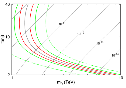
(a) $\kappa=0.09$

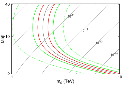
(b) $\kappa=0.05$

Figure 1: Our numerical results on ${\rm Br}(\mu\to e\gamma)$ and the lightest Higgs boson mass in the MSSM-like semi-constrained NMSSM, case 1. The diagonal gray contours are the contours for the predicted branching ratios of $\mu\to e\gamma$. The diagonal solid and dotted red lines are the current limit and the near-future expected sensitivity of ${\rm Br}(\mu\to e\gamma)$, respectively. The current limits of the $\mu\to 3e$ and $\mu$-$e$ conversion rates are also shown by the corresponding values of ${\rm Br}(\mu\to e\gamma)$ as the solid light-blue and dark-blue lines, respectively. The near-future expected reach of ${\rm Br}(\mu\to 3e)$ is shown by the dotted light-blue lines, and that of the $\mu$-$e$ conversion at COMET and Mu2e is shown by the dotted dark-blue lines. The gray line is the contour for the 126 GeV Higgs boson mass. The regions between the two red curves, the two solid green curves and the two dotted green curves are the areas where the Higgs boson mass is in the ranges, 125-127, 124-128 and 120-130 ${\rm GeV}$, respectively. We assume $m_{0}=M_{1/2}$ in the figures. The input parameters at the SUSY scale are $\lambda=0.1,A_{\kappa}=-50~{}{\rm(GeV)}$ and we take $A_{0}=-500~{}{\rm(GeV)}$ at the GUT scale. The right-handed neutrino Majorana masses are taken to be $M_{\nu}=5.0\times 10^{14}~{}{\rm(GeV)}$.

Numerical Results

Our numerical results for ${\rm Br}(\mu\to e\gamma)$ and the Higgs boson mass in the case 1 are given in Figs. 1 (a) and (b). In the figures (a) and (b), $\kappa$ at the SUSY scale is taken to be 0.09 and 0.05, respectively. The rest of the input parameters are taken to be the same in the two figures, and the input SUSY parameters are $\lambda=0.1,A_{\kappa}=-50~{}{\rm(GeV)}$ at the SUSY scale and $A_{0}=-500~{}{\rm(GeV)}$ at the GUT scale. We take $m_{0}=M_{1/2}$, and the right-handed neutrino Majorana mass is taken to be $M_{\nu}=5.0\times 10^{14}~{}{\rm(GeV)}$. The reason for the choice of this value of $M_{\nu}$ is that for $M_{\nu}=5.0\times 10^{14}~{}{\rm(GeV)}$, the largest neutrino Yukawa coupling becomes ${\cal O}(1)$, as can be seen from Eq. (2.27). For smaller values of $M_{\nu}$, the LFV rates become smaller since the off-diagonal entries of the slepton mass matrix become smaller, see Eq. (3.15).

In the figures, we plot contours for constant values of ${\rm Br}(\mu\to e\gamma)$. Since ${\rm Br}(\mu\to e\gamma)$ is roughly proportional to $\tan^{2}\beta/m_{0}^{4}$ for $A_{0}\ll m_{0}$ and $\tan\beta\gg 1$, the dependence of the contours on $\tan\beta$ and $m_{0}$ are simple. In the case of the MSSM $+\nu_{R}$ model, similar results are known in literature [17, 18, 19, 24, 25, 20, 36].

In the figures, we also show the current limit and the near-future expected sensitivity of ${\rm Br}(\mu\to e\gamma)$ by the solid and dotted diagonal red lines, respectively. The current limits of the $\mu\to 3e$ and $\mu$-$e$ conversion rates are also shown by the corresponding values of ${\rm Br}(\mu\to e\gamma)$ in the figures as the solid light-blue and dark-blue lines, respectively. Similarly, the near-future expected reach of ${\rm Br}(\mu\to 3e)$ is shown by the dotted light-blue lines, and that of the $\mu$-$e$ conversion at the COMET and Mu2e experiments is shown by the dotted dark-blue lines. Once the PRISM/PRIME experiment is realized, it is expected to go beyond the COMET/Mu2e sensitivity by about two orders of magnitude, and the full region in the figures will be covered for this particular choice of the input parameters.

Also shown in Figs. 1 (a) and (b) are the contours for the lightest Higgs boson mass. From the figures, we find that smaller $\kappa$ makes the Higgs boson mass smaller. We have numerically confirmed that the difference in the Higgs boson mass mainly comes from the values of $\kappa$, and the difference in the values of the other parameters like $A_{\lambda}$ are not very important for the difference in the predictions for the Higgs boson mass. This dependence of the Higgs boson mass on $\kappa$ can be understood from Eq. (4.8). Namely, large $\kappa$ makes the $(3,3)$ element of ${\cal M}^{2}_{S,{\rm Tree}}$ larger and the mixing between the MSSM Higgses and the singlet Higgs, which makes a negative contribution to the lightest Higgs boson mass, smaller.

From the figures, we find that there is a parameter region which is favored from the Higgs boson mass measurement where the predicted value of ${\rm Br}(\mu\to e\gamma)$ is within reach of the near-future experiment even if $m_{0}$ is as large as $\sim 4$ TeV. In addition, the near-future experiments Mu3e, COMET and Mu2e can probe the SUSY mass scale up to $\sim 5$ TeV for our sample parameters. The reach will be extended further if the PRISM/PRIME experiment is carried out.

We here comment on the dependence of the Higgs boson mass on $\kappa$. In the figures, we take $\kappa$ only down to 0.05. For smaller values of $\kappa$, for example, $\kappa\lesssim 0.03$ for $\lambda=0.1$, the Higgs boson mass sharply decreases for decreasing $\kappa$. This sharp $\kappa$ dependence comes from the factor $(\lambda/\kappa)^{2}$ in the third term of the right-hand side of Eq. (4.8). If we take smaller value of $\lambda$, this sharp decrease of $\kappa$ happens at smaller value of $\kappa$, and hence we can take smaller $\kappa$ as well.

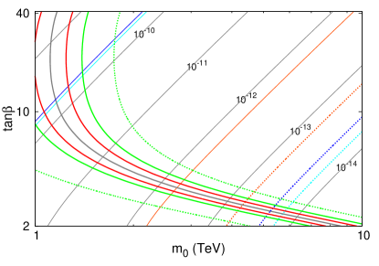
Figure 2: The numerical results for ${\rm Br}(\mu\to e\gamma)$ and the lightest Higgs boson mass in the MSSM $+\nu_{R}$ model. The diagonal gray contours are the contours for the predicted branching ratios of $\mu\to e\gamma$. The meanings of the diagonal red/light-blue/dark-blue solid/dotted lines, gray line, red curves, two solid green curves, and two dotted green curves are the same as in Fig. 1. We assume $m_{0}=M_{1/2}$ in the figure. We take $A_{0}=-500~{}{\rm(GeV)}$ at the GUT scale and assume $\mu>0$. The right-handed neutrino Majorana masses are taken to be $M_{\nu}=5.0\times 10^{14}~{}{\rm(GeV)}$.

The difference between the above results and the result in the case of the MSSM $+\nu_{R}$ model can become clearer if we compare Figs. 1 (a) and (b) with the prediction in the MSSM $+\nu_{R}$ model for similar input parameters. In Fig. 2 we show the prediction for ${\rm Br}(\mu\to e\gamma)$ in the MSSM $+\nu_{R}$ model with the boundary conditions at the GUT scale, Eqs. (2.3)–(2.6) together with the conditions at the GUT scale $M_{1/2}=m_{0}$ and $(m_{N}^{2})_{ij}=m_{0}^{2}\delta_{ij}$, where $(m_{N}^{2})_{ij}$ $(i,j=1,\ldots,3)$ is the soft SUSY breaking mass-squared matrix for the right-handed neutrinos. We take $A_{0}=-500~{}{\rm(GeV)}$ at the GUT scale and assume $\mu>0$. We also take the same neutrino masses and mixing parameters as in Figs. 1 (a) and (b), as well as the same right-handed neutrino Majorana masses which are taken to be $M_{\nu}=5.0\times 10^{14}~{}{\rm(GeV)}$. By comparing Figs. 1 (a), (b) with Fig. 2, we see little difference for the prediction for ${\rm Br}(\mu\to e\gamma)$ for given values of $\tan\beta$ and $m_{0}$ $(=M_{1/2})$, but the region favored from the Higgs boson mass slightly changes. For example, for a fixed value of $\tan\beta=10$, the value of ${\rm Br}(\mu\to e\gamma)$ predicted from the fixed value of the Higgs boson mass at $m_{H}=126$ GeV in the MSSM $+\nu_{R}$ model is $\sim 10^{-10}$ for this particular choice of input parameters, while in the case of Figs. 1 (a) and (b), the corresponding values are $\sim 6\times 10^{-11}$ and $\sim 2\times 10^{-11}$, respectively. We therefore conclude that in the NMSSM $+\nu_{R}$ model, the predicted value of ${\rm Br}(\mu\to e\gamma)$ favored from the Higgs boson mass can slightly change from the MSSM $+\nu_{R}$ model.

Case 2

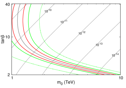
(a) $A_{\lambda}(M_{{\rm GUT}})=-5000~{}({\rm GeV})$

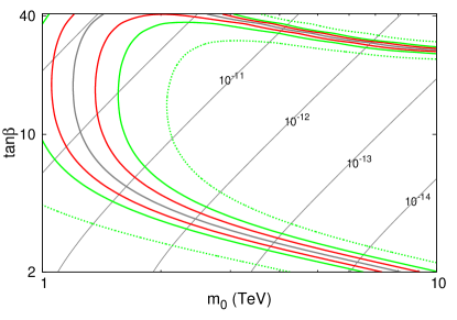
(b) $A_{\lambda}(M_{{\rm GUT}})=-2500~{}({\rm GeV})$

Figure 3: Our numerical results on ${\rm Br}(\mu\to e\gamma)$ and the lightest Higgs boson mass in the MSSM-like semi-constrained NMSSM, case 2. The diagonal gray contours are the contours for the predicted branching ratios of $\mu\to e\gamma$. The meanings of the diagonal red/light-blue/dark-blue solid/dotted lines, gray line, red curves, two solid green curves, and two dotted green curves are the same as in Fig. 1. We assume $m_{0}=M_{1/2}$ in the figures. The input parameters at the SUSY scale are $\lambda=0.1,A_{\kappa}=-50~{}{\rm(GeV)}$ and we take $A_{0}=-500~{}{\rm(GeV)}$ at the GUT scale. The right-handed neutrino Majorana masses are taken to be $M_{\nu}=5.0\times 10^{14}~{}{\rm(GeV)}$.

In this case, if we are to use Eq. (4.9), the value of $\kappa$ is determined to be, similarly to the case 1,

$$\kappa=\frac{\lambda}{\sin{2\beta}}-\frac{A_{\lambda}}{2s}~{}.$$ (5.6)

Similarly to the reasoning in the case 1, the equation above implies that if $\tan\beta$ or $\lambda$ is too large, the $\kappa$ parameter at higher scale blows up and becomes non-perturbative. Therefore, if we are to use Eq. (4.9), we need small $\lambda$ and small $\tan{\beta}$, but this choice makes the Higgs boson mass very similar to the MSSM case and hence is not very interesting. We therefore do NOT use Eq. (4.9) in the case 2, either.

Numerical Results

In Figs. 3 (a) and (b), we give our numerical results for ${\rm Br}(\mu\to e\gamma)$ and the lightest Higgs boson mass in the case 2. In the figures (a) and (b), $A_{\lambda}$ at the GUT scale is taken to be $-5000$ GeV and $-2500$ GeV, respectively. The rest of the input parameters are taken to be the same in the two figures, and the input SUSY parameters are $\lambda=0.1,A_{\kappa}=-50{\rm~{}(GeV)}$ at the SUSY scale, and $A_{0}=-500{\rm~{}(GeV)}$ at the GUT scale. We take $m_{0}=M_{1/2}$, and $M_{\nu}=5.0\times 10^{14}~{}{\rm(GeV)}$.

In the figures, we plot contours for the constant values of ${\rm Br}(\mu\to e\gamma)$. The behaviors are very similar to the case 1. Also shown are the favored regions from the Higgs boson mass and the current and near-future expected sensitivities of the $\mu\to e\gamma$, $\mu\to 3e$ and $\mu$-$e$ conversion rates, similarly to Figs. 1 (a) and (b).

From the figures, we find that only in Fig. 3 (b), there is an extra Higgs-mass favored parameter space at the region where $\tan\beta$ and $m_{0}~{}(=M_{1/2})$ are both large. This difference between the two figures mainly comes from the difference in the value of $\kappa$, and the differences in the other parameters like $A_{\lambda}$ enter only indirectly through the value of $\kappa$ in the prediction for the Higgs boson mass.

We now explain why the changes in the input value of $A_{\lambda}$ at the GUT scale affect the value of $\kappa$ at the SUSY scale.

To do so, we first explain the dependence of $\kappa$ on $m_{0}~{}(=M_{1/2})$ and $\tan\beta$ with fixed value of $A_{\lambda}(M_{\rm GUT})$. Below we will show that $\kappa$ becomes smaller for larger $m_{0}$ and for larger $\tan\beta$ at the region $\tan\beta\gg 1$ in the parameter space shown in Figs. 3 (a) and (b). At the upper-right region of Fig. 3 (b), the value of $\kappa$ becomes $\kappa\lesssim 0.03$, where the Higgs boson mass decreases relatively quickly for decreasing $\kappa$, as discussed at the end of the discussion for the case 1 in this section. In the parameter region shown in Fig. 3 (a), the value of $\kappa$ is larger than 0.03, and hence this relatively fast decrease does not happen. Then we have to explain why $\kappa$ is smaller in Fig. 3 (b). This is because $A_{\lambda}(M_{\rm SUSY})$ is larger in Fig. 3 (b) since $A_{\lambda}(M_{\rm GUT})$ is larger. The relation between $A_{\lambda}(M_{\rm SUSY})$ and $\kappa$ are given by $\kappa=(B_{\rm eff}-A_{\lambda})/s$ and hence larger $A_{\lambda}$ means smaller $\kappa$.

Let us discuss the change in $\kappa$ for different $m_{0}~{}(=M_{1/2})$ for fixed values of $\tan\beta$ and $A_{\lambda}(M_{\rm GUT})$. The value of $A_{\lambda}$ at the SUSY scale is given by solving the RGE,

$$16\pi^{2}\frac{d}{dt}A_{\lambda} =4|\kappa|^{2}A_{\kappa}+8|\lambda|^{2}A_{\lambda}+6{\rm Tr}(Y_{U}^{\dagger}T_{U})+6{\rm Tr}(Y_{D}^{\dagger}T_{D})+2{\rm Tr}(Y_{E}^{\dagger}T_{E})+2{\rm Tr}(Y_{N}^{\dagger}T_{N})$$

$$\quad+6g_{2}^{2}M_{2}+\frac{6}{5}g_{1}^{2}M_{1}~{}.$$ (5.7)

For our sample parameters, $A_{\lambda}(M_{{\rm SUSY}})$ becomes larger for larger $m_{0}~{}(=M_{1/2})$ and fixed $\tan\beta$. Therefore, for a fixed value of $\tan{\beta}$, larger $m_{0}~{}(=M_{1/2})$ makes $\kappa$ smaller through the relation, $\kappa=(B_{{\rm eff}}-A_{\lambda})/s$.

Next, we discuss the dependence of $\kappa$ on $\tan\beta$, fixing the values of $m_{0}~{}(=M_{1/2})$ and $A_{\lambda}$ at the GUT scale. Since here we are mainly interested in the difference at large $\tan\beta$ region, in this paragraph we assume $\tan\beta\gg 1$. For large $\tan\beta$, $A_{\lambda}(M_{\rm SUSY})$ becomes larger for larger $\tan\beta$ since the fourth term of the right-hand side of Eq. (5.7), which involves the bottom Yukawa coupling, becomes more important. This increase in $A_{\lambda}(M_{\rm SUSY})$ for larger $\tan\beta$ makes $\kappa$ smaller for fixed $m_{0}$ since $\kappa=(B_{{\rm eff}}-A_{\lambda})/s$. Another reason which makes $\kappa$ smaller for larger $\tan\beta$ comes from the values of $\mu_{{\rm eff}}$ and $B_{{\rm eff}}$, although this effect is less important for large $\tan\beta$. The values of $\mu_{{\rm eff}}$ and $B_{{\rm eff}}$ at the SUSY scale are obtained by solving the tadpole conditions, and the solutions at the tree-level are,

$$\mu_{{\rm eff}}^{2} =\frac{m^{2}_{H_{d}}-m^{2}_{H_{u}}\tan^{2}{\beta}}{\tan^{2}{\beta}-1}-\frac{1}{2}M^{2}_{Z}~{},$$ (5.8)

$$B_{{\rm eff}} =\frac{1}{2\mu_{{\rm eff}}}(m^{2}_{H_{u}}+m^{2}_{H_{d}}+2\mu^{2}_{{\rm eff}}+v^{2}\lambda^{2})\sin{2\beta}~{}.$$ (5.9)

Both $\mu_{{\rm eff}}$ and $B_{{\rm eff}}$ become smaller for larger $\tan{\beta}$ for our sample parameters. From the relation $\mu_{{\rm eff}}=\lambda s$, a smaller $\mu_{{\rm eff}}$ means a smaller $s$ for fixed $\lambda$. From $\kappa=(B_{{\rm eff}}-A_{\lambda})/s$, the variation of $\kappa$ comes from that of $s~{}(=\mu_{{\rm eff}}/\lambda)$ and that of $B_{{\rm eff}}$. For our sample parameters, since the decrease in $B_{{\rm eff}}$ due to increase in $\tan\beta$ has a larger effect on $\kappa$ than that of $s$, $\kappa$ becomes smaller for larger $\tan\beta$.

As for ${\rm Br}(\mu\to e\gamma)$, also in the case 2, we find that there is a parameter region which is favored from the Higgs boson mass and in which the predicted value of ${\rm Br}(\mu\to e\gamma)$ is within reach of near-future experiment even if $m_{0}\sim 4~{}({\rm TeV})$, which has not yet been probed at the LHC.

6 Summary and Discussions

In this paper, we have studied the cLFV in the semi-constrained NMSSM+$\nu_{R}$ model, taking into account the recent results on the Higgs boson mass determination. We have considered the boundary conditions at the GUT scale to be MSSM-like and semi-constrained in the sense that the SUSY breaking parameters $A_{\lambda},A_{\kappa},m_{S}^{2}$ which are specific to the NMSSM are not necessarily equal to $A_{0},A_{0},m_{0}^{2}$, respectively. We have considered two cases: in one case the parameters ($s,\ A_{\lambda},\ m^{2}_{S}$) are determined from the tadpole conditions, which we call the case 1, while in the other case ($s,\ \kappa,\ m^{2}_{S}$) are determined from other input parameters, which we call the case 2.

One of the advantages of the NMSSM is that the tree-level lightest Higgs boson mass can be taken to be larger than that of the MSSM by taking a large value of $\lambda$. In addition to this effect, there is another new effect in the Higgs boson sector of the NMSSM, namely, we also have to take into account the mixing with the singlet Higgs. This mixing can decrease the Higgs boson mass depending on the parameters. In the semi-constrained scenario we have considered, we find it is difficult to realize both large $\lambda$ and small mixing with the singlet at the same time. Hence in this paper we have assumed a small $\lambda~{}(\sim 0.1)$ which makes the mixing with the singlet small.

In the case 1, we have obtained the results similar to those in the MSSM $+~{}\nu_{R}$ model. We have also shown that the Higgs-boson-mass favored parameter region depends on the value of $\kappa$. As the case 2, we have considered the case where the $\kappa$ parameter is not an input parameter but is a parameter determined from other parameters via the tadpole conditions, and we have obtained a partly different favored region from the case 1. In both cases, we have shown that in the NMSSM+$\nu_{R}$ model there is a parameter region in which the predicted value of ${\rm Br}(\mu\to e\gamma)$ is so large that the $\mu\to e\gamma$ decay can be observable at the near-future experiment even if the SUSY mass scale is about 4 TeV. The reach will be improved further by the near-future experiments, Mu3e, COMET, Mu2e and PRISM/PRIME.

Several comments are in order. In this paper we have taken the input SUSY mass parameter $m_{0}(=M_{1/2})$ as high as $\gtrsim$ 1 TeV. This choice makes the squarks and gluino as heavy as multi-TeV, whose possibility is still not excluded by any experiments including the LHC [1]. The price we have to pay is that it is difficult to explain the muon $g-2$ anomaly in terms of SUSY if we take the multi-TeV SUSY particle mass scenario, and that we have to introduce the so-called “little hierarchy” between the weak scale and the SUSY scale. In particular, some fine-tuning is necessary in order to keep the Higgs boson mass protected from large radiative corrections. Nevertheless, in SUSY models the cancellation between the bosonic and fermionic loop contributions to the Higgs-boson mass-squared is automatic at the scales much higher than the SUSY breaking scale, which decreases the degree of fine-tuning significantly compared to the non-SUSY minimal standard model and makes SUSY models still attractive.

References

- [1] K. A. Olive et al. [Particle Data Group Collaboration], Chin. Phys. C 38, 090001 (2014).
- [2] J. Adam et al. [MEG Collaboration], Phys. Rev. Lett. 110, 201801 (2013)
- [3] S. P. Martin, Adv. Ser. Direct. High Energy Phys. 21, 1 (2010) [hep-ph/9709356].
- [4] Y. Okada, M. Yamaguchi and T. Yanagida, Prog. Theor. Phys. 85, 1 (1991).
- [5] J. R. Ellis, G. Ridolfi and F. Zwirner, Phys. Lett. B 257, 83 (1991).
- [6] H. E. Haber and R. Hempfling, Phys. Rev. Lett. 66, 1815 (1991).
- [7] U. Ellwanger, C. Hugonie and A. M. Teixeira, Phys. Rept. 496, 1 (2010)
- [8] P. Minkowski, Phys. Lett. B 67, 421 (1977).
- [9] T. Yanagida, Conf. Proc. C 7902131, 95 (1979).
- [10] M. Gell-Mann, P. Ramond and R. Slansky, Conf. Proc. C 790927, 315 (1979)
- [11] I. Gogoladze, N. Okada and Q. Shafi, Phys. Lett. B 672, 235 (2009) [arXiv:0809.0703 [hep-ph]].
-
[12]
R. N. Mohapatra,
Phys. Rev. Lett. 56, 561 (1986);
R. N. Mohapatra and J. W. F. Valle, Phys. Rev. D 34, 1642 (1986). - [13] F. Deppisch and J. W. F. Valle, Phys. Rev. D 72, 036001 (2005) [hep-ph/0406040].
- [14] Z. Maki, M. Nakagawa and S. Sakata, Prog. Theor. Phys. 28, 870 (1962).
- [15] J. A. Casas and A. Ibarra, Nucl. Phys. B 618, 171 (2001) [hep-ph/0103065].
- [16] T. Blazek and S. F. King, Phys. Lett. B 518, 109 (2001)
- [17] A. Ibarra and C. Simonetto, JHEP 0908, 113 (2009)
- [18] R. Alonso, G. Isidori, L. Merlo, L. A. Munoz and E. Nardi, JHEP 1106, 037 (2011)
- [19] J. h. Park, Phys. Rev. D 89, 095005 (2014)
- [20] J. Hisano, T. Moroi, K. Tobe and M. Yamaguchi, Phys. Rev. D 53, 2442 (1996)
- [21] T. P. Cheng and L. F. Li, Phys. Rev. Lett. 38, 381 (1977).
- [22] S. T. Petcov, Sov. J. Nucl. Phys. 25, 340 (1977) [Yad. Fiz. 25, 641 (1977)] [Erratum-ibid. 25, 698 (1977)] [Erratum-ibid. 25, 1336 (1977)].
- [23] S. M. Bilenky, S. T. Petcov and B. Pontecorvo, Phys. Lett. B 67, 309 (1977).
- [24] F. Borzumati and A. Masiero, Phys. Rev. Lett. 57, 961 (1986).
- [25] J. Hisano, T. Moroi, K. Tobe, M. Yamaguchi and T. Yanagida, Phys. Lett. B 357, 579 (1995)
- [26] A. M. Baldini, F. Cei, C. Cerri, S. Dussoni, L. Galli, M. Grassi, D. Nicolo and F. Raffaelli et al., arXiv:1301.7225 [physics.ins-det].
- [27] Y. Kuno and Y. Okada, Rev. Mod. Phys. 73, 151 (2001) [hep-ph/9909265].
- [28] T. Aushev, W. Bartel, A. Bondar, J. Brodzicka, T. E. Browder, P. Chang, Y. Chao and K. F. Chen et al., arXiv:1002.5012 [hep-ex].
- [29] A. Blondel et al., Letter of Intent to PSI, December 2011.
- [30] R. Kitano, M. Koike and Y. Okada, Phys. Rev. D 66, 096002 (2002) [Erratum-ibid. D 76, 059902 (2007)] [hep-ph/0203110].
- [31] D. Bryman et al. [COMET Collaboration], J-PARC Proposal P21 (2007).
- [32] R. M. Carey et al. [Mu2e Collaboration] Fermilab Letter of Intent (2007).
- [33] Y. Kuno et al. [PRISM/PRIME Collaboration], J-PARC Letter of Intent (2006).
- [34] Y. Kuno [COMET Collaboration], PTEP 2013, 022C01 (2013).
- [35] D. Brown [Mu2e Collaboration], Nucl. Phys. Proc. Suppl. 248-250, 41 (2014).
-
[36]
See, for example,
J. Hisano and D. Nomura,
Phys. Rev. D 59, 116005 (1999)
[hep-ph/9810479];
S. Davidson and A. Ibarra, JHEP 0109, 013 (2001) [hep-ph/0104076];
S. Baek, T. Goto, Y. Okada and K. i. Okumura, Phys. Rev. D 64, 095001 (2001) [hep-ph/0104146];
F. Deppisch, H. Pas, A. Redelbach, R. Ruckl and Y. Shimizu, Eur. Phys. J. C 28, 365 (2003) [hep-ph/0206122];
S. Pascoli, S. T. Petcov and W. Rodejohann, Phys. Rev. D 68, 093007 (2003) [hep-ph/0302054];
S. T. Petcov, S. Profumo, Y. Takanishi and C. E. Yaguna, Nucl. Phys. B 676, 453 (2004) [hep-ph/0306195];
A. Masiero, S. K. Vempati and O. Vives, New J. Phys. 6, 202 (2004) [hep-ph/0407325];
A. Brignole and A. Rossi, Nucl. Phys. B 701, 3 (2004) [hep-ph/0404211];
E. Arganda and M. J. Herrero, Phys. Rev. D 73, 055003 (2006) [hep-ph/0510405];
J. Hisano, M. Nagai, P. Paradisi and Y. Shimizu, JHEP 0912, 030 (2009) [arXiv:0904.2080 [hep-ph]];
M. Hirsch, F. R. Joaquim and A. Vicente, JHEP 1211, 105 (2012) [arXiv:1207.6635 [hep-ph]];
M. Cannoni, J. Ellis, M. E. Gomez and S. Lola, Phys. Rev. D 88, no. 7, 075005 (2013) [arXiv:1301.6002 [hep-ph]];
T. Moroi, M. Nagai and T. T. Yanagida, Phys. Lett. B 728, 342 (2014) [arXiv:1305.7357 [hep-ph]];
A. J. R. Figueiredo and A. M. Teixeira, JHEP 1401, 015 (2014) [arXiv:1309.7951 [hep-ph]];
J. Sato and M. Yamanaka, Phys. Rev. D 91, 055018 (2015) [arXiv:1409.1697 [hep-ph]];
T. Goto, Y. Okada, T. Shindou, M. Tanaka and R. Watanabe, Phys. Rev. D 91, 033007 (2015) [arXiv:1412.2530 [hep-ph]].