Ultrashort-period MS eclipsing systems. New observations and light curve solutions of six NSVS binaries

Abstract

We carried out photometric and low-resolution spectral observations of six eclipsing ultrashort-period binaries with MS components. The light curve solutions of the Rozhen observations show that all targets are overcontact systems. We found well-defined empirical relation “period – semi-major axis” for the short-period binaries and used it for estimation of the global parameters of the targets. Our results revealed that NSVS 925605 is quite interesting target: (a) it is one of a few contact binaries with M components; (b) it exhibits high activity (emission in H$\alpha$ line, X-ray emission, large cool spots, non-Planck energy distribution); (c) its components differ in temperature by 700 K. All appearances of high magnetic activity and huge fillout factor (0.7) of NSVS 925605 might be assumed as a precursor of the predicted merging of close magnetic binaries. Another unusual binary is NSVS 2700153 which reveals considerable long-term variability.

1 Introduction

The short-period binaries with non-degenerate components are important objects for the astrophysics, especially for the understanding of the very late evolutional stages of the binaries connected with the processes of mass and angular momentum loss, merging or fusion of the stars, etc. But their structure and evolution remains unsolved problem in stellar astrophysics due to poor statistics. There are two reasons for this insufficiency.

Firstly, the period distribution of binaries reveals a very sharp decline in the number of short period systems below 0.27 days (Drake et al., 2014). Systems with periods around the short-period limit of 0.22 day (Rucinski, 1992) were extremely rare: the fraction of ultrashort period objects was estimated to only 0.26 $\%$ of the total number of the large number of contact systems (Drake et al., 2014). Secondly, the faintness of the late short binaries makes them difficult targets for detailed study. As a result, although M-dwarfs form the most common stellar population in our Galaxy ($\sim$ 70 $\%$ by number, Henry et al., 1999), their intrinsic faintness is barrier to study their binary characteristics.

Lately, a hypothesis appeared that the very short period low-mass binaries could merge via “magnetic braking“ and if a substantial amount of mass remains in orbit around the primary, it would form a disk in which planets could be produced, particularly hot Jupiters (Martin et al., 2011).

Fortunately, the modern large stellar surveys during the last decade allowed to discover binaries with shorter and shorter periods (Rucinski, 2007; Pribulla et al., 2009; Weldrake et al., 2004; Maceroni & Rucinski, 1997; Dimitrov & Kjurkchieva, 2010; Norton et al., 2011; Nefs et al., 2012; Davenport et al., 2013; Lohr et al., 2014; Qian et al., 2014; Drake et al., 2014, etc.).

This paper presents our observations and light curve solutions of six ultrashort-period binaries (whose periods are below 0.23 d).

2 Selection of targets

Using own approach (Dimitrov, 2009) for searching for stellar variability we reviewed the NSVS database (Woźniak et al., 2004) and found around 300 ultrashort-period candidates with W UMa-type light curves. More than 100 of them were removed as probable $\delta$ Sct stars due to their small infrared colors (temperatures $T>6000$ K). We carried out short test observations of the rest candidates and established that most of them were not variable stars. In such a way we managed to separate sample of about forty ultrashort-period candidates from the NSVS survey appropriate for follow-up observations at Rozhen observatory ($\delta>-10\degr$). Our study of one of them (BX Tri) was already published (Dimitrov & Kjurkchieva, 2010).

Table 1 reveals the coordinates and magnitudes of six other targets from this sample: four of them are newly discovered eclipsing stars while two of them are identified with objects from the lists of ultrashort-period binaries of Norton et al. (2011) and Lohr et al. (2014) based on the SuperWASP photometric survey (Pollacco et al., 2006).

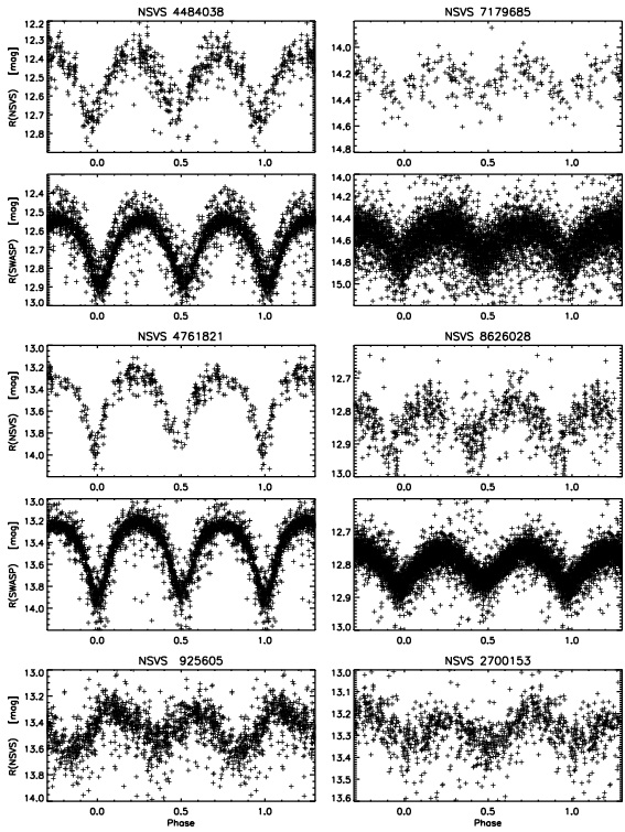
Figure 11: Folded light curves based on the NSVS and SuperWASP observations of the targets

Besides photometric data for all six targets in the NSVS database we found also data of four of them in the SuperWASP archive (Butters et al., 2010). The periodogram analysis of these low-precise but numerous data allowed us to determine their ephemeris (Table 1). Figure 11 presents the folded curves of the targets corresponding to their old photometric data.

Table 1: List of our ultrashort-period targets

Target	NSVS ID	$\alpha$	$\delta$	$R_{\rm{NSVS}}$	Period	References
		[2000]	[2000]	[mag]	[d]
1	4484038	05 54 16.99	+44 25 34.1	12.50	0.2185	Norton et al. (2011)
2	7179685	06 46 06.47	+36 20 21.1	14.90	0.2097	new
3	4761821	08 01 50.03	+47 14 33.8	13.10	0.2175	Norton et al. (2011)
4	2700153	13 43 51.43	+63 04 22.8	12.48	0.2285	new
5	925605	14 01 46.37	+77 16 38.7	13.73	0.2176	new
6	8626028	21 16 26.81	+25 17 36.2	13.78	0.2174	new

3 Rozhen observations and data reduction

The follow-up CCD photometry of the targets in $VRI$ bands was carried out with the three telescopes of Rozhen National Astronomical Observatory (Table 2). The 2-m RCC telescope is equipped with VersArray CCD camera (1340 $\times$ 1300 pixels, 20 $\mu$m/pixel, field of 5.35 $\times$ 5.25 arcmin). The 60-cm Cassegrain telescope is equipped with FLI PL09000 CCD camera (3056 $\times$ 3056 pixels, 12 $\mu$m/pixel, field of 17.1 $\times$ 17.1 arcmin). The 50/70-cm Schmidt telescope has FoV around 1^∘ and is equipped with CCD camera FLI PL 16803, 4096 $\times$ 4096 pixels, 9 $\mu$m/pixel size.

Table 2: Journal of the Rozhen photometric observations

Date	Filter	Exp. [s]	Number	Telescope
NSVS 4484038
2010 Feb 24	$VI$	120,60	16,16	60-cm
2010 Dec 08	$VI$	120,60	90,90	60-cm
2011 Jan 08	$VI$	120,90	87,86	60-cm
NSVS 7179685
2009 Sept 29	$R$	120	40	60-cm
2009 Sept 30	$R$	120	132	60-cm
2009 Oct 23	$VRI$	120,120,120	50,50,50	60-cm
2010 Mar 06	$R$	120	95	60-cm
2010 Mar 12	$I$	120	310	60-cm
2011 Jan 01	$V$	40	434	2-m
NSVS 4761821
2009 Nov 19	$R$	120	50	60-cm
2011 Jan 01	$VI$	120,60	103,103	60-cm
2011 Jan 06	$VI$	120,120	85,85	60-cm
2011 Jan 13	$VI$	120,120	18,16	60-cm
NSVS 2700153
2010 May 16	$VI$	120,120	8,20	60-cm
2010 June 20	$VI$	120,120	86,85	60-cm
2010 Nov 21	$VI$	120,120	21,21	60-cm
2011 Jan 17	$VI$	120,120	82,82	Shmidt
2011 Jan 18	$V$	120	125	Shmidt
2011 Jan 19	$I$	120	155	Shmidt
NSVS 925605
2009 June 05	$R$	120	100	60-cm
2009 June 06	$R$	120	100	60-cm
2009 July 27	$V$	120	91	60-cm
2009 Aug 26	$VRI$	120,60,60	50,50,50	60-cm
2009 Aug 27	$VRI$	120,60,60	60,60,60	60-cm
NSVS 8626028
2009 Aug 26	$VRI$	120,60,60	50,50,50	60-cm
2009 Aug 27	$VRI$	120,60,60	59,60,60	60-cm

Standard stars of Landolt (1992) and standard fields of Stetson (2000) were used for transition from instrumental system to standard photometric system.

The standard IDL procedures (adapted from DAOPHOT) were used for reduction of the photometric data. More than 5 standard stars were chosen in the observed fields of each target by the requirement to be constant within 0.015 mag during the all observational runs and in all filters. Table 7 presents their $V$, $B-V$, $V-R$, and $V-I$ determined by our observations (for the targets they correspond to phase 0.25) as well as their $J-K$ colors from the 2MASS catalog.

Figures 1-6 present the follow-up Rozhen photometry of our targets. Table 8 presents a sample of the Rozhen photometric data (the full table is available in the online version of the article, see Supporting Information).

We calculated times of the observed light minima by the method described in Pribulla et al. (2012). Table 9 contains their $HJD$(Min), Epoch, and $O-C$.

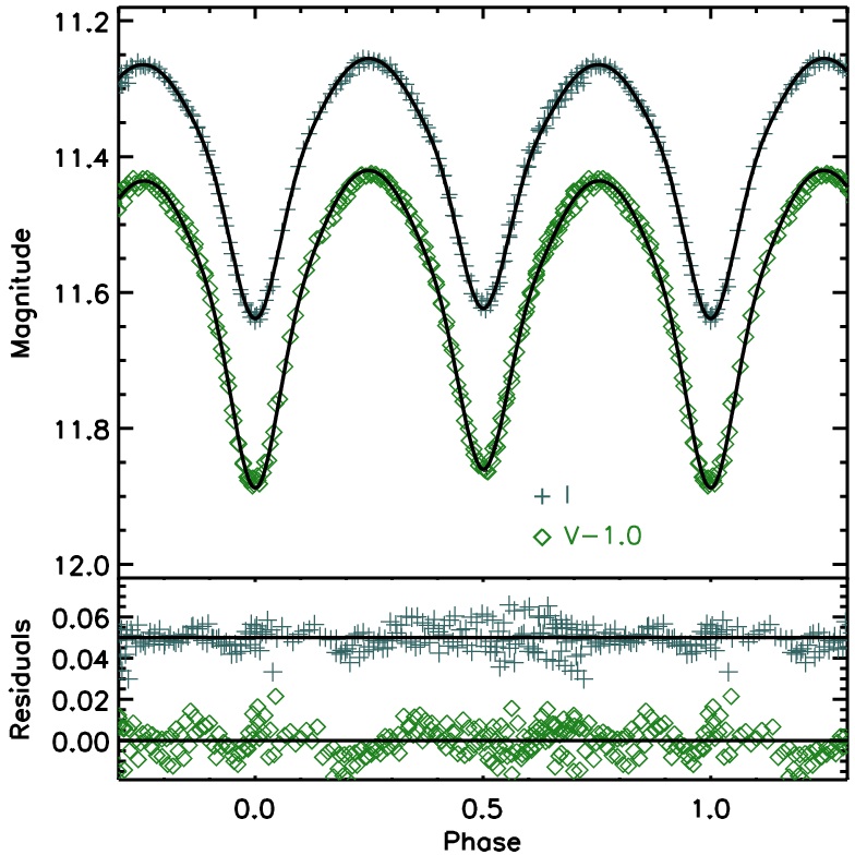
Figure 1: Top: the folded light curves of NSVS 4484038 and their fits (continuous lines); Bottom: the corresponding residuals. The photometric data in some filters are shifted vertically by different number for a better visibility. Color version of this figure is available in the online journal.

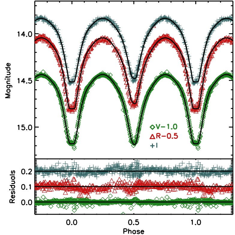
Figure 2: Same as Fig. 1 for NSVS 7179685.

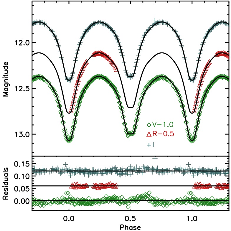
Figure 3: Same as Fig. 1 for NSVS 4761821.

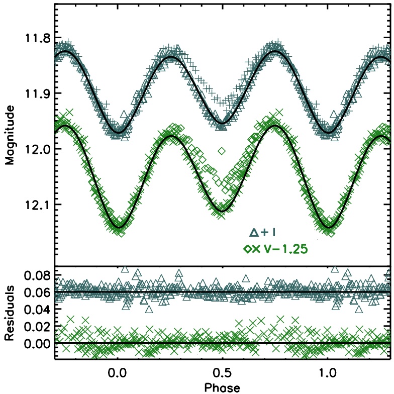
Figure 4: Same as Fig. 1 for NSVS 2700153.

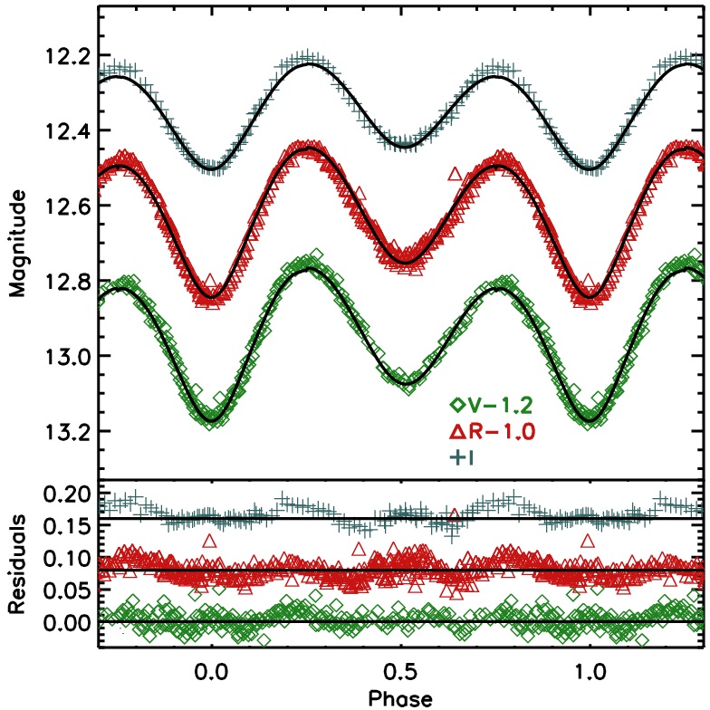
Figure 5: Same as Fig. 1 for NSVS  925605.

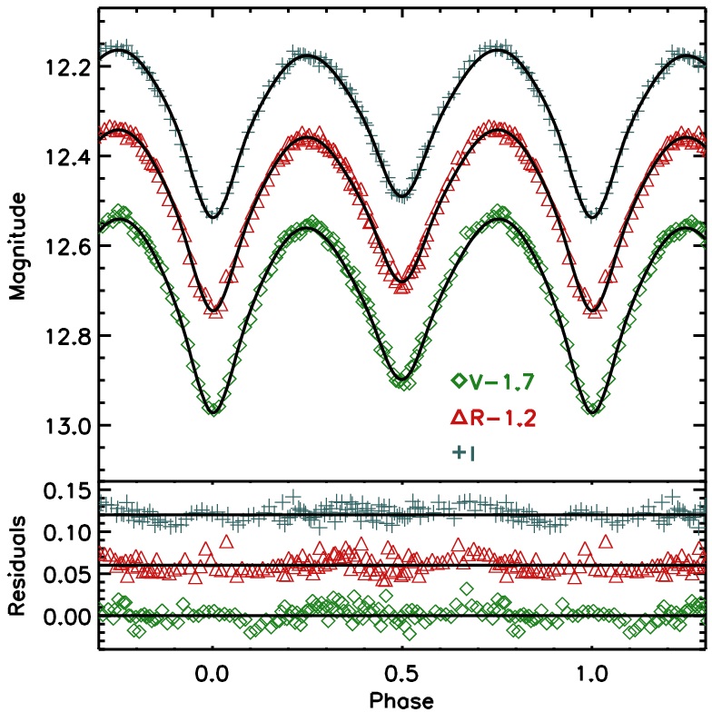
Figure 6: Same as Fig. 1 for NSVS 8626028.

We obtained low-resolution spectra (Fig. 7) during 5 nights in Feb-May 2011 by the 2-m RCC telescope equipped with focal reducer FoReRo-2. We used grism with 300 lines/mm that allows resolution 5.223 Å/pixel in the range 5000-7000 Å. These low-resolution spectra do not allow radial velocity measurement but are useful indicators of the temperature and stellar activity.

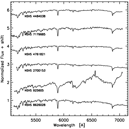
Figure 7: The low-resolution spectra of the targets around the H$\alpha$ line

4 Light curve solutions

The photometric data (Figs. 1-6) implied that our targets are contact or overcontact systems that was expected for their ultra-short orbital periods.

Table 3: The 2MASS color indices $J-K$ and corresponding mean temperatures $T_{\rm{m}}$ of the targets

Target	NSVS 4484038	NSVS 7179685	NSVS 4761821	NSVS 2700153	NSVS  925605	NSVS 8626028
$J-K$	$0.590\pm 0.030$	$0.798\pm 0.033$	$0.651\pm 0.033$	$0.635\pm 0.037$	$0.863\pm 0.028$	$0.769\pm 0.028$
$T_{\rm{m}}$	$4950\pm 150$	$4040\pm 190$	$4690\pm 130$	$4730\pm 200$	$3490\pm 250$	$4200\pm 180$

We carried out modeling of the Rozhen photometric data by the code PHOEBE (Prśa & Zwitter, 2005) using the following procedure.

We determined in advance the mean temperatures $T_{\rm{m}}$ of the binaries (Table 3) by their infrared color indices $(J-K)$ from the 2MASS catalog and the calibration color-temperature of Tokunaga (2000). The ”spectral” temperatures of the targets obtained by comparison of their low-resolution spectra (Fig. 7) with those of standard stars with known temperatures, were almost the same as those of the values of $T_{\rm{m}}$ in Table 3.

Firstly we assumed $T_{1}^{0}=T_{\rm{m}}$ and searched for solutions for fixed $T_{1}^{0}$ and $q^{0}=1$ varying the ephemeris, secondary temperature $T_{2}$, orbital inclination $i$ and potentials $\Omega_{1,2}$.

We adopted coefficients of gravity brightening 0.32 and reflection 0.5 appropriate for late stars. The linear limb-darkening coefficients were interpolated from the values of Van Hamme (1993). In order to reproduce the O’Connell effect we added cool spots on the components and varied their parameters: longitude $\beta$, latitude $\lambda$, angular size $\alpha$ and temperature factor $k=T_{\rm{sp}}/T_{1}$. To obtain a good fit in all colors a third light was necessary for some targets.

As a result of the first stage of the light curve solution we obtained initial values $T_{2}^{0}$, $i^{0}$ and $\Omega_{1,2}^{0}$ as well as the ephemeris and spot parameters for each target. Further we determined the mass ratio applying q-search method. We calculated the normalized $\chi^{2}$ for two-dimensional grid ($i,\log q$) consisting of values of $i$ within the $10^{\circ}$-range around the value $i^{0}$ with step $0.5^{0}$ and $q$ values $0.15,0.20,...,0.95,1.00,1/0.95,1/0.90,...,1/0.20,1/0.15$ ($T_{1}^{0}$, $T_{2}^{0}$ and spot parameters were fixed). In this way we obtained $\chi^{2}_{\rm{min}}(1)$ corresponding to the first approximation ($i^{1},q^{1}$). Further this procedure was repeated around the pair ($i^{1},q^{1}$) for finer grid corresponding to 10 times smaller step of $q$ and 5 times smaller step of $i$. The obtained $\chi^{2}_{\rm{min}}(2)$ corresponded to the second approximation ($i^{2},q^{2}$), etc. Thus we reach to the absolute minimum with $\chi^{2}_{\rm{min}}(abs)\sim 1$ corresponding to the final values ($i^{\rm{f}},q^{\rm{f}}$).

The diagrams ($i,\log q$) exhibit that the solution ambiguity rapidly increases with the decreasing of the orbital inclination (Fig. 8). Maceroni et al (1985) has reached to the same result by other procedure.

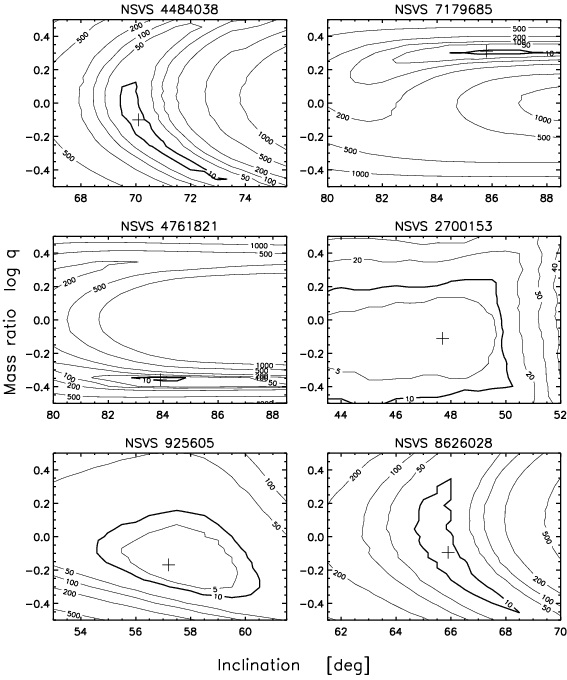
Figure 8: Diagrams $i$, $\log q$ with isolines corresponding to different values of the normalized $\chi^{2}$, the symbols $"+"$ mark the positions of $\chi^{2}_{\rm{min}}(abs)$

Further we searched for the best fit for fixed $i^{\rm{f}}$, $q^{\rm{f}}$, ephemerides and spot parameters, varying $T_{2}$, $\Omega_{1,2}$ and third light $l_{3}(V,R,I)$. Finally, we calculated $T_{1}$ and $T_{2}$. For this aim we developed the approach of Coughlin et al. (2011)

$$T_{1}=T_{\rm{m}}+\frac{\Delta T}{c+1}$$ (1)

$$T_{2}=T_{1}-\Delta T$$ (2)

where $c=l_{2}/l_{1}$ and $\Delta T$ (difference of temperatures of the components) are determined from the PHOEBE solution.

Table 4 contains the final values of all determined parameters: period $P$; initial epoch $HJD_{0}$; orbital inclination $i$; temperatures of the components $T_{1,2}$; potentials of the components $\Omega_{1,2}$; fill-out factor $FF$; spot parameters; third light contribution in the different colors $l_{3}(V,R,I)$. The errors of the parameters in Table 4 are the formal PHOEBE values.

The synthetic light curves corresponding to the parameters from Table 4 are shown in Figs. 1-6 as continuous lines.

Table 4: Results from the light curve solutions

Parameter		NSVS 4484038	NSVS 7179685	NSVS 4761821	NSVS 2700153	NSVS  925605	NSVS 8626028
$P$	[d]	0.218493	0.209740	0.217513	0.228456	0.217629	0.217407
		$\pm 0.000001$	$\pm 0.000001$	$\pm 0.000001$	$\pm 0.000001$	$\pm 0.000001$	$\pm 0.000001$
$HJD_{0}$	[d]	5539.479711	5104.528662	5563.438743	5368.312230	4988.575181	5070.408406
+2450000		$\pm 0.000035$	$\pm 0.000011$	$\pm 0.000020$	$\pm 0.000114$	$\pm 0.000028$	$\pm 0.000051$
$i$	[°]	70.1	85.5	83.8	47.8	57.2	65.9
		$\pm 0.1$	$\pm 0.2$	$\pm 0.1$	$\pm 0.4$	$\pm 0.2$	$\pm 0.1$
$q=M_{2}/M_{1}$		0.792	2.128	0.432	0.775	0.678	0.805
		$\pm 0.002$	$\pm 0.007$	$\pm 0.001$	$\pm 0.003$	$\pm 0.003$	$\pm 0.002$
$T_{1}$	[K]	5000	4100	4685	4785	3813	4318
		$\pm 43$	$\pm 32$	$\pm 32$	$\pm 51$	$\pm 51$	$\pm 27$
$T_{2}$	[K]	4897	3979	4696	4689	3135	4095
		$\pm 41$	$\pm 29$	$\pm 29$	$\pm 40$	$\pm 65$	$\pm 22$
$r_{1}$		0.407	0.326	0.464	0.409	0.474	0.418
$r_{2}$		0.364	0.456	0.318	0.364	0.408	0.380
$l_{2}/l_{1}$		0.727	1.731	0.479	0.709	0.221	0.592
$\Omega_{1}=\Omega_{2}$		3.365	5.316	2.707	3.343	2.930	3.330
		$\pm 0.004$	$\pm 0.006$	$\pm 0.006$	$\pm 0.007$	$\pm 0.010$	$\pm 0.004$
$FF$		0.0857	0.193	0.136	0.071	0.702	0.207
$Spot_{1}$		primary	primary	–	–	primary	primary
$\lambda$	[°]	115	270	–	–	115	225
$\beta$	[°]	90	90	–	–	63	70
$\alpha$	[°]	13	15	–	–	16	9
$\kappa$		0.9	0.9	–	–	0.84	0.9
$Spot_{2}$		–	–	–	–	secondary	primary
$\lambda$	[°]	–	–	–	–	178	310
$\beta$	[°]	–	–	–	–	90	90
$\alpha$	[°]	–	–	–	–	18	11
$T_{\rm{Spot2}}$	[K]	–	–	–	–	0.8	0.9
$l_{3}(V)$		0.015	0.012	0.014	–	0.089	0.036
		$\pm 0.004$	$\pm 0.003$	$\pm 0.010$	–	$\pm 0.012$	$\pm 0.011$
$l_{3}(R)$		–	–	–	–	0.078	0.048
		–	–	–	–	$\pm 0.010$	$\pm 0.009$
$l_{3}(I)$		0.112	0.007	–	0.069	0.293	0.056
		$\pm 0.003$	$\pm 0.004$	–	$\pm 0.008$	$\pm 0.011$	$\pm 0.005$

The parameter mass ratio deserves a special attention. Although its determination through analysis of the light-curve is an ambiguous approach compared with that by radial velocity solution, the rapid rotation of the components of the ultrashort-period binaries is serious obstacle to obtain precise spectral mass ratio from measurement of their highly broadened and blended spectral lines (Bilir et al., 2005; Dall & Schmidtobreick, 2005). Contrariwise, tests have revealed that photometric mass ratios are more reliable than spectroscopic ones for totally eclipsing W UMa-type stars and are sufficiently reliable for partially eclipsing systems (Maceroni & van’t Veer, 1996) because their eclipse depths depend strongly on the geometrical parameters and the mass ratio $q$. Hence, the obtained photometric $q$ values of our targets may be considered with a confidence.

5 Analysis of the results

The analysis of the light curve solutions led us to several conclusions.

(a)

All targets are overcontact (OC) binaries. The fill-out factor of NSVS 925605 is huge (Fig. 9).

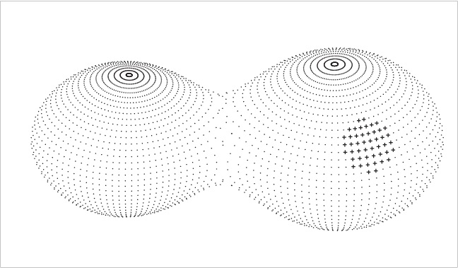
Figure 9: 3D configuration of the strongly overcontact target NSVS 925605.

(b)

The mass ratios of four targets are within the narrow range 0.68–0.8 while NSVS 7179685 and NSVS 4761821 have components which masses differ around 2 times. Just they are with total eclipses and thus with most precise photometric mass ratio.

(c)

The differences between the temperatures of the components of the targets are up to 220 K, that is expected for overcontact systems. The only exception is NSVS 925605 which cool components differ by nearly 700 K (although the big fill-out factor).

(d)

NSVS 7179685 is the only target which more massive star is the cooler component. We do not know overcontact binary with orbital period below 0.21 d with such a property.

(e)

NSVS  925605 is rare case of overcontact ultrashort period binary consisting of M dwarfs.

(f)

NSVS 2700153 revealed considerable long-term variability during our observations (Fig. 4): the secondary minimum was shallower than the primary one in June 2010, but they became almost equal in depth in Jan 2011. Parameters in Table 4 correspond to the light curve solution from Jan 2011.

(g)

NSVS 925605 shows high activity: emission in H$\alpha$ line (Fig. 7) from its chromosphere; X-ray emission from the corona (it is the only X-ray source among our six targets identified as 1RXS J140139.8+771643); large cool photospheric spot. The considerable contribution of third light, especially in $I$ color (Table 4), cannot be explained by blurring because there is not nearby star within 1 arcsec from this target. The reason could be non-Planck distribution of its energy. All appearances of high magnetic activity and huge fillout factor of NSVS 925605 might be interpreted in the light of the hypothesis of Martin et al. (2011) as a precursor of the merging of close magnetic binaries.

6 Global parameters of the targets

Due to lack of RV-curve solutions we had to use empirical relations for determination of the global characteristics of our targets. For this aim we built a diagram period–semi-major axis ($P,a$) on the base of 14 binaries with $P<0.27$ d which have radial velocity solution and modern light curve solution (Table 5). Their distribution was approximated by parabola

$$a=-1.154+14.633\times P-10.319\times P^{2}\qquad[R\sun]$$ (3)

where $a$ is in solar radii and $P$ in days. The standard deviation of the fit is 0.05 R$\sun$ and we assume this value as a mean error of $a$ for our targets with periods around 0.22 days.

Such a relation is expected for contact and overcontact binaries of MS late stars for which $R_{1}+R_{2}\approx a$ and $R\sim M^{k}$ where $k\approx 1$. Then the third Kepler law leads to $a\sim P$ that is similar to the almost linear dependence (3) for periods of about 0.22 d (Fig. 10).

The ($P,a$) relation (3) corresponds to the following relation “period–mass” for short-period binaries

$$M=\frac{0.0134}{P^{2}}\left(-1.154+14.633\times P-10.319\times P^{2}\right)^{3}\,[M\sun]$$ (4)

where $M$ is the total mass of the binary.

It is important to know is there a lower limit of the period-axis relation (3). Very recently Drake et al. (2014) modeled binaries with extremely short periods by configurations consisting of white dwarf and dM star. They are stable non-accreting WD+MS systems which differ from the accretion induced variability in CV variables. We added these five systems (Table 5) on our diagram ($P,a$). It is interesting that their semiaxes, and respective masses, are almost the same (within the errors) while the orbital periods are quite different. The WD+dM models (blue asterisk) of four of these binaries fall away from the line approximating the relation ($P,a$) of binaries with MS components (red line). It is visible that the dependence of the semiaxis of these extremely short-period binaries on the period (blue continuous line) is considerably weaker. One of them, CSS J001242.4+130809, has 2 models: WD+dM and dM+dM (Table 5). Its dM+dM model as well as the longest-period target, CSS J090119.2+114254, fall just on the line period–axis of our MS binaries (Fig. 10). This may imply that such configurations are more appropriate for these two targets. The low-resolution spectroscopy of the extremely short-period binaries (Drake et al., 2014) revealed the presence of Balmer emission and Ca H+K emission typical for late dwarfs and strong local magnetic fields.

Table 5: Semi-major axes of short-period binaries from spectral studies

Star	$P_{\rm{orb}}$	$M_{1}+M_{2}$	$a$	References
CSS J090826.3+123648*	0.1392	0.80	1.049	Drake et al. (2014)
CSS J111647.8+294602*	0.1462	0.75	1.061	Drake et al. (2014)
CSS J081158.6+311959*	0.1562	0.70	1.083	Drake et al. (2014)
CSS J001242.4+130809*	0.1641	0.80	1.171	Drake et al. (2014)
CSS J001242.4+130809	0.1641	0.41	0.937	Drake et al. (2014)
CSS J090119.2+114254*	0.1867	0.70	1.222	Drake et al. (2014)
BX Tri	0.1926	0.77$\pm$0.03	1.284$\pm$0.022	Dimitrov & Kjurkchieva (2010)
BW3 V38	0.1984	0.85$\pm$0.11	1.356$\pm$0.085	Maceroni & Montalban (2004)
SDSS J001641-000925	0.1986	0.88$\pm$0.08	1.372$\pm$0.057	Davenport et al. (2013)
GSC 1387-475	0.2178	0.94$\pm$0.03	1.492$\pm$0.019	Rucinski & Pribulla (2008)
CC Com	0.2211	1.09$\pm$0.02	1.585$\pm$0.011	Pribulla et al. (2007)
1SWASP J160156.04+202821.6	0.2265	1.43$\pm$0.06	1.761$\pm$0.033	Lohr et al. (2014)
V523 Cas	0.2337	1.13$\pm$0.04	1.663$\pm$0.025	Rucinski et al. (2003)
RW Com	0.2373	1.18$\pm$0.03	1.704$\pm$0.060	Pribulla et al. (2009)
BI Vul	0.2518	1.45	1.899	Maceroni & van’t Veer (1996)
1SWASP J150822.80-054236.9	0.2601	1.62$\pm$0.10	2.013$\pm$0.065	Lohr et al. (2014)
VZ Psc	0.2612	1.46$\pm$0.06	1.950$\pm$0.040	Hrivnak et al. (1995)
V803 Aql	0.2634	1.58	2.014	Maceroni & van’t Veer (1996)
FS Cra	0.2636	1.51	1.984	Maceroni & van’t Veer (1996)
44 Boo=i Boo	0.2678	1.47	1.987	Lu et al. (2001)

Note: Stars with WD+dM model are marked with asterisk.

We used the empirical relation (3) to obtain the semi-major axes $a$ of our targets and further the masses $M_{1,2}$, radii $R_{1,2}$, and luminosities $L_{1,2}$ of their components in solar units; bolometric and visual absolute magnitudes $M_{\rm{bol}}$ and $M_{V}$ of the targets; distance $d$ in parsecs and orbital angular momenta $J_{\rm{orb}}$ (by the expression of Popper & Ulrich, 1977). Table 6 contains the values of the obtained global parameters.

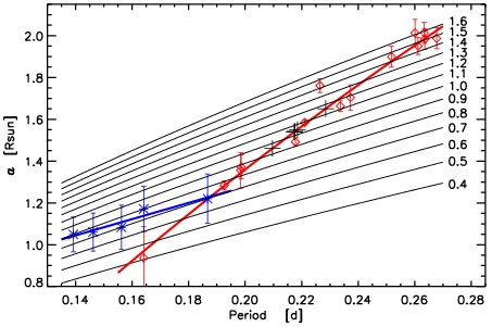
Figure 10: Diagram period – semi-major axis for short-period binaries. The thin black lines represent the isolines of binary (total) mass. The positions of the stars from Table 6 are marked by red diamonds while those of our targets are marked by black pluses. The red line exhibits the empirical relation described by equation (3). The blue line presents empirical relation for WD+dM binaries, marked with blue asterisk. Color version of this figure is available in the online journal.

Table 6: Global parameters of the targets

Name	$a$	$R_{1}$	$M$	$M_{1}$	$L_{1}$	$M_{\rm{bol}}$	$d$	$J_{\rm{orb}}$
		$R_{2}$		$M_{2}$	$L_{2}$	$M_{V}$
NSVS 4484038	1.55	0.63$\pm$0.02	1.01	0.56$\pm$0.06	0.23$\pm$0.02	5.73$\pm$0.11	200	0.151
	$\pm$0.05	0.57$\pm$0.02	$\pm$0.10	0.45$\pm$0.04	0.17$\pm$0.02	5.928	$\pm$12	$\pm$0.034
NSVS 7179685	1.461	0.48$\pm$0.02	0.95	0.30$\pm$0.03	0.06$\pm$0.01	6.68$\pm$0.13	428	0.118
	$\pm$0.05	0.67$\pm$0.02	$\pm$0.09	0.65$\pm$0.06	0.10$\pm$0.01	7.284	$\pm$26	$\pm$0.027
NSVS 4761821	1.541	0.71$\pm$0.02	1.04	0.72$\pm$0.07	0.23$\pm$0.02	6.00$\pm$0.10	248	0.137
	$\pm$0.05	0.49$\pm$0.02	$\pm$0.10	0.32$\pm$0.03	0.11$\pm$0.01	6.397	$\pm$12	$\pm$0.030
NSVS 2700153	1.650	0.67$\pm$0.02	1.15	0.65$\pm$0.06	0.22$\pm$0.02	5.81$\pm$0.11	267	0.190
	$\pm$0.05	0.60$\pm$0.02	$\pm$0.11	0.50$\pm$0.05	0.16$\pm$0.02	6.060	$\pm$14	$\pm$0.042
NSVS 925605	1.542	0.73$\pm$0.02	1.04	0.62$\pm$0.06	0.11$\pm$0.01	6.82$\pm$0.12	154	0.155
	$\pm$0.05	0.64$\pm$0.02	$\pm$0.10	0.42$\pm$0.04	0.024$\pm$0.005	8.020	$\pm$9	$\pm$0.034
NSVS 8626028	1.540	0.63$\pm$0.02	1.04	0.57$\pm$0.06	0.13$\pm$0.01	6.40$\pm$0.10	184	0.159
	$\pm$0.05	0.57$\pm$0.02	$\pm$0.10	0.47$\pm$0.04	0.09$\pm$0.01	7.904	$\pm$9	$\pm$0.035

The orbital angular momenta of the targets (Table 6) are considerably smaller than those of the RS CVn binaries and detached systems which have $\log J_{\rm{orb}}\geq+0.08$. They are smaller also than those of the ordinary contact systems which have $\log J_{\rm{orb}}\geq-0.5$. The obtained $J_{\rm{orb}}$ values are bigger only than those of the shortest-period CVs of SU UMa type.

7 Conclusions

We found well-defined empirical relation “period – semi-major axis” for the short-period binaries and used it for estimation of the global parameters of six ultrashort-period targets.

One of them, NSVS 925605, with huge fill-out factor and another peculiar characteristics (consisting of M components with high activity and non-Planck energy distribution) probably is at stage of merging.

Our results revealed that all six ultrashort-period targets with periods 0.20–0.23 days are overcontact systems. At the same time the short-period binaries BX Tri and BW3 V38 with periods below 0.20 have detached configurations. Nefs et al. (2012) spectroscopically confirmed another detached system with a 0.18 day period containing an M-dwarf. It is worth to study which parameters determine the stellar configuration (detached, contact or overcontact) of the ultrashort-period binaries.

Appendix A Additional information

Table 7: Colors of the targets and their standard stars

Star	ID	$V$	$B-V$	$V-R$	$V-I$	$J-K$
	GSC1.2(2.3)	[mag]	[mag]	[mag]	[mag]	[mag]
NSVS 4484038
Var	2924-0179	12.43	0.71	0.25	1.17	0.59
St1	2924-2161	12.86	1.00	0.40	1.31	0.69
St2	2924-1407	12.68	1.23	0.70	1.93	1.08
St3	2924-1435	13.23	0.60	0.16	0.78	0.37
St4	2924-0641	12.02	1.87	0.68	1.88	1.07
St5	2924-1202	11.79	0.86	0.13	0.69	0.34
St6	2924-1060	12.94	0.97	0.46	1.40	0.75
NSVS 7179685
Var	N8BM016247	15.44	0.45	0.91	1.61	0.80
St1	2448-0250	13.42	0.65	0.71	1.20	0.63
St2	N8BN012958	13.63	0.35	0.48	0.77	0.34
St3	2448-0995	13.29	1.34	0.77	1.42	0.74
St4*	N8BM016279	15.19	0.46	0.72	1.23	0.64
St5*	N8BM016265	15.64	0.28	0.71	1.29	0.69
St6*	N8BM016250	15.38	-0.20	0.43	0.69	0.24
St7*	N8BM016262	15.20	0.08	0.55	0.96	0.48
St8*	N8BM016256	15.82	0.10	0.55	0.95	0.44
NSVS 4761821
Var	3408-0735	13.37	1.06	0.76	1.60	0.65
St1	3408-1475	11.58	0.82	0.74	1.44	0.49
St2	3408-0617	13.51	0.66	0.61	1.15	0.33
St3	3408-0431	12.59	0.69	0.83	1.72	0.74
St4	3408-0459	13.26	0.54	0.63	1.14	0.30
St5	3408-2017	13.54	0.73	0.66	1.18	0.31
NSVS 2700153
Var	4174-0776	13.19	0.82	0.71	1.37	0.64
St1	4174-1064	12.42	0.71	0.39	1.00	0.43
St2	4174-0970	12.99	0.68	0.42	0.95	0.43
St3	4174-0772	13.29	0.42	0.41	0.83	0.30
St4	4174-0696	12.07	0.53	0.43	0.83	0.31
St5	4174-0764	13.76	0.35	0.46	0.96	0.41
St6	4174-0526	14.03	0.46	0.37	1.02	0.46
NSVS 925605
Var	4558-0304	13.96	1.00	0.52	1.75	0.86
St1	4558-0096	14.09	0.19	-0.11	0.16	0.30
St2	4558-0054	13.01	0.53	-0.12	0.18	0.33
St3	4558-0448	13.93	0.60	0.07	0.48	0.56
St4	4558-0340	14.35	0.39	-0.03	0.33	0.46
St5	4558-0500	14.09	0.43	-0.02	0.32	0.37
St6	4558-2326	15.58	0.99	0.42	1.29	0.82
NSVS 8626028
Var	2190-2019	14.23	0.66	0.69	2.07	0.77
St1	2190-1524	10.06	0.40	0.17	1.05	0.27
St2	2190-1134	12.42	0.50	0.27	1.23	0.32
St3	2190-1456	12.76	0.51	0.28	1.26	0.35
St4	2190-0565	12.49	1.12	0.82	2.59	1.09
St5	2190-2044	11.70	1.08	0.54	1.79	0.69

* Standard stars used for the observations with the 2-m telescope

Table 8: Rozhen photometric data. This is a sample of the full table, which is available with the online version of the article (see Supporting Information). The number of the target is the same as in Table 1.

Target	Filter	$HJD$	Magnitude	Error
		[d]	[mag]	[mag]
1	$V$	2455252.267213	12.8632	0.0059
1	$I$	2455252.269054	11.6127	0.0054
1	$V$	2455252.270188	12.8297	0.0059
1	$I$	2455252.272028	11.5911	0.0053
…	…	…	…	…
2	$R$	2455104.580844	14.5421	0.0175
2	$R$	2455104.582256	14.5606	0.0177
2	$R$	2455104.583680	14.5489	0.0177
2	$R$	2455104.585104	14.5417	0.0178
…	…	…	…	…

Table 9: Times of the observed eclipse minima.

$HJD$(Min)	Filter	Type of	Epoch	$O-C$
[d]		minimum		[d]
NSVS 4484038
2455539.479830	V	Min I	0	0.000563
2455539.479669	I	Min I	0	-0.000174
2455539.589299	V	Min II	0	0.001572
2455539.589183	I	Min II	0	0.001041
2455570.287555	V	Min I	141	-0.001048
2455570.287666	I	Min I	141	-0.000540
2455570.397084	V	Min II	141	0.000236
2455570.397060	I	Min II	141	0.000126
NSVS 7179685
2455104.632827	R	Min II	0	-0.003361
2455105.472144	R	Min II	4	-0.001659
2455105.576676	R	Min I	5	-0.003271
2455128.544335	V	Min II	114	0.002112
2455128.543839	R	Min II	114	-0.000253
2455128.543751	I	Min II	114	-0.000672
2455128.648854	V	Min I	115	0.000439
2455128.648414	R	Min I	115	-0.001659
2455128.648348	I	Min I	115	-0.001974
2455262.463012	R	Min I	753	0.000620
2455268.335791	I	Min I	781	0.000901
2455268.440937	I	Min II	781	0.002217
2455563.545264	V	Min II	2188	0.002918
2455563.649773	V	Min I	2189	0.001197
NSVS 4761821
2455563.547579	V	Min II	0	0.000365
2455563.546281	I	Min II	0	-0.005603
2455563.656336	V	Min I	1	0.000367
2455563.656667	I	Min I	1	0.001889
2455568.441653	V	Min I	23	0.000509
2455568.441644	I	Min I	23	0.000468
2455568.550426	V	Min II	23	0.000585
2455568.550388	I	Min II	23	0.000411
NSVS 2700153
2455368.313740	V	Min I	0	0.006631
2455368.313195	I	Min I	0	0.004246
2455368.425320	V	Min II	0	-0.004959
2455368.426162	I	Min II	0	-0.001274
2455579.518952	V	Min II	924	-0.003699
2455579.518799	I	Min II	924	-0.004368
2455580.548178	V	Min I	929	0.001440
2455580.660175	V	Min II	929	-0.008325
2455581.575046	I	Min II	933	-0.003743
2455581.690325	I	Min I	934	0.000858
NSVS  925605
2454988.467268	R	Min II	-1	0.004147
2454989.443816	R	Min I	4	-0.008639
2454989.555544	R	Min II	4	0.004749
2455040.368512	V	Min I	238	-0.010890
2455070.297199	V	Min II	375	0.010704
2455070.296609	R	Min II	375	0.007993
2455070.296099	I	Min II	375	0.005650
2455070.402749	V	Min I	376	-0.004296
2455070.402535	R	Min I	376	-0.005280
2455070.402487	I	Min I	376	-0.005500
2455071.272856	V	Min I	380	-0.006176
2455071.272715	R	Min I	380	-0.006824
2455071.272511	I	Min I	380	-0.007761
2455071.385397	V	Min II	380	0.010948
2455071.384643	R	Min II	380	0.007483
2455071.383811	I	Min II	380	0.003660
NSVS 8626028
2455070.516938	V	Min I	0	-0.000789
2455070.516287	R	Min I	0	-0.003783
2455070.516218	I	Min I	0	-0.004101
2455071.496252	V	Min I	5	0.003730
2455071.496096	R	Min I	5	0.003013
2455071.496085	I	Min I	5	0.002962
2455071.604069	V	Min II	5	-0.000347
2455071.603989	R	Min II	5	-0.000715
2455071.604153	I	Min II	5	0.000039

References

- Bilir et al. (2005) Bilir S., Karatas Y., Demircan O., Eker Z., 2005, MNRAS, 357, 497
- Butters et al. (2010) Butters O.W., et al., 2010, A&A, 520L, 10
- Coughlin et al. (2011) Coughlin J.L., Lo’pez-Morales M., Harrison T.E., Ule N., Hoffman D.I., 2011, AJ, 141, 78
- Dall & Schmidtobreick (2005) Dall T., Schmidtobreick L., 2005, A&A, 429, 625
- Davenport et al. (2013) Davenport J.R.A., et al., 2013, ApJ, 764, 62
- Dimitrov (2009) Dimitrov D.P., 2009, Bulg. AJ, 12, 49
- Dimitrov & Kjurkchieva (2010) Dimitrov D.P., Kjurkchieva D.P., 2010, MNRAS, 406, 2559
- Drake et al. (2014) Drake A.J., et al., 2014, ApJ, 790, 157
- Hrivnak et al. (1995) Hrivnak B.J., Guinan E.F., Lu W., 1995, ApJ, 455, 300
- Henry et al. (1999) Henry T.J., et al., 1999, ApJ, 512, 864
- Landolt (1992) Landolt A., 1992, AJ, 104, 340
- Lohr et al. (2014) Lohr M.E., Hodgkin S.T., Norton A.J., Kolb U.C., 2014, A&A 563A, 34
- Lu et al. (2001) Lu W., Rucinski S.M., Ogloza W., 2001, AJ, 122, 402
- Maceroni & Montalban (2004) Maceroni C., Montalban J., 2004, A&A, 426, 577
- Maceroni & Rucinski (1997) Maceroni C., Rucinski S.M., 1997, PASP, 109, 782
- Maceroni & van’t Veer (1996) Maceroni C., van’t Veer F., 1996, A&A, 311, 523
- Maceroni et al (1985) Maceroni C., Milano L., Russo G., 1985, MNRAS, 217, 843
- Martin et al. (2011) Martin E.L., Spruit H.C., Tata R., 2011, A&A, 535, 50
- Nefs et al. (2012) Nefs S.V., et al., 2012, MNRAS 425, 950
- Norton et al. (2011) Norton A.J., et al., 2011, A&A, 528A, 90
- Pollacco et al. (2006) Pollacco D.L., et al. 2006, PASP, 118, 1407
- Popper & Ulrich (1977) Popper D., Ulrich R., 1977, ApJ, 212, L131
- Pribulla et al. (2007) Pribulla T., et al., 2007, AJ, 133, 1977
- Pribulla et al. (2009) Pribulla T., et al., 2009, AJ 137, 3646
- Pribulla et al. (2012) Pribulla T., et al., 2012, AN 333, 754
- Prśa & Zwitter (2005) Prśa A., Zwitter T., 2005, ApJ, 628, 426
- Qian et al. (2014) Qian S.-B., Jiang L.-Q., Zhu L.-Y., Zejda M., Mikulášek Z., Fernández-Lajús E., Liu N.-P., 2014, CoSka, 43, 290
- Rucinski (1992) Rucinski S.M., 1992, AJ, 103, 960
- Rucinski (2007) Rucinski S.M., 2007, MNRAS, 382, 393
- Rucinski & Pribulla (2008) Rucinski S.M., Pribulla T., 2008, MNRAS, 388, 1831
- Rucinski et al. (2003) Rucinski S.M. et al, 2003, AJ, 125, 3258
- Stetson (2000) Stetson P., 2000, PASP, 112, 925
- Tokunaga (2000) Tokunaga A.T., in Allen’s astrophysical quantities, 4th ed. Edited by Arthur N. Cox, New York, AIP Press, Springer, 2000, p. 143
- Van Hamme (1993) Van Hamme W., 1993, AJ, 106, 2096
- Weldrake et al. (2004) Weldrake D.T.F., Sackett P.D., Bridges T.J., Freeman K.C., 2004, AJ, 128, 736
- Woźniak et al. (2004) Woźniak P.R., et al., 2004, AJ, 127, 2436