Synchro-curvature radiation of charged particles
in the strong curved magnetic fields

Abstract

It is generally believed that the radiation of relativistic particles in a curved magnetic field proceeds in either the synchrotron or the curvature radiation modes. In this paper we show that in strong curved magnetic fields a significant fraction of the energy of relativistic electrons can be radiated away in the intermediate, the so-called synchro-curvature regime. Because of the persistent change of the trajectory curvature, the radiation varies with the frequency of particle gyration. While this effect can be ignored in the synchrotron and curvature regimes, the variability plays a key role in the formation of the synchro-curvature radiation. Using the Hamiltonian formalism, we find that the particle trajectory has the form of a helix wound around the drift trajectory. This allows us to calculate analytically the intensity and energy distribution of prompt radiation in the general case of magnetic bremsstrahlung in the curved magnetic field. We show that the transition to the limit of the synchrotron and curvature radiation regimes is determined by the relation between the drift velocity and the component of the particle velocity perpendicular to the drift trajectory. The detailed numerical calculations, which take into account the energy losses of particles, confirm the principal conclusions based on the simplified analytical treatment of the problem, and allow us to analyze quantitatively the transition between different radiation regimes for a broad range of initial pitch angles. These calculations demonstrate that even very small pitch angles may lead to significant deviations from the spectrum of the standard curvature radiation when it is formally assumed that a charged particle moves strictly along the magnetic line. We argue that in the case of realization of specific configurations of the electric and magnetic fields, the gamma-ray emission of the pulsar magnetospheres can be dominated by the component radiated in the synchro-curvature regime.

1. Introduction

The energy distribution and intensity of radiation of a charged particle moving in the magnetic field with a relativistic speed is determined by the curvature of its trajectory. The trajectory in the curved magnetic field has a structure of a helix wound along the so-called drift trajectory, which describes the particle motion averaged over the fast oscillations. Thus, the curvature of the trajectory is formed by the curvature of the helix itself and the curvature of the drift trajectory; they are determined by the strength and the curvature of the magnetic field, respectively. If the main contributor is the curvature of the helix (i.e., the bending of the drift trajectory can be neglected), the radiation is defined by the strength of the magnetic field. This is the case of the synchrotron radiation. On the other hand, if the helix is stretched (i.e., the particle moves along the drift trajectory with a little wobbling around it), the main contribution to the radiation is due to the curvature of the drift trajectory. This is the case of the curvature radiation, which is determined by curvature of the drift trajectory . Obviously, the synchrotron and curvature radiation regimes are approximations that work with a high precision as long as the curvatures of the helix and the drift trajectory differ significantly. However, when they are comparable their joint action may result in features that are significantly different from those described by the standard synchrotron and curvature radiation formalism. These two contributions to the curvature can reinforce or extinguish each other, and therefore cause a significant variability of the curvature of the particle trajectory. It results, in turn, in a radiation that varies with the frequency of the particle gyration. The observer detects the time-averaged energy distribution of this promptly variable radiation, which appears rather different from the spectra of emission produced in the synchrotron or curvature radiation regimes.

A few attempts have been made in the past to study this intermediate regime of radiation, which we, following Cheng & Zhang (1996), call synchro-curvature radiation. However the approaches and assumptions used in the previous treatments of the problem (Cheng & Zhang, 1996; Harko & Cheng, 2002) are generally not self-consistent. For example, in the paper of Cheng & Zhang (1996), where the particle motion is introduced a priori (“by hand”), the square of the velocity is not conserved. The more recent results of Harko & Cheng (2002) also seem not correct. In particular, the acceleration in this work is not variable as it follows from the solution of equations that describe the particle trajectories (compare the formula given by Equation (5) in their paper and the expression given by Equation (40) in the present work). On the other hand, we cannot fail to mention the apparently underrated work of Sobolev (2006), where the author has thoroughly treated the problem of radiation of particles in the magnetic field. Some principal results and conclusions of this paper are in a good agreement with the results of Section 2 of the present work, although they have been obtained using a rather different computational approach to the problem. However, these results are of rather theoretical interest because the energy losses of particles are ignored.

In this work, using the Hamiltonian formalism, we solve the equations of the motion of a charged particle in the azimuthally symmetric magnetic field. This allows us to self-consistently describe the local properties of the particle trajectory with a time-dependent curvature, and calculate the time-averaged spectrum of radiation in an arbitrary magnetic field. The analytical solutions derived in an approximation that ignores energy losses of electrons provide a useful tool for understanding of distinct feature of the synchro-curvature radiation, and analyzing the conditions of its transition to the limits of synchrotron and curvature regimes.

On the other hand, for the quantitative description of propagation and radiation of particles, one has to treat the energy losses of electrons properly. For this reason, we have performed numerical integration of the equations of motion in the dipole magnetic field, taking into account the radiation reaction force. The dipole magnetic field can be used as a good approximation for the strong magnetic field in the vicinity of compact objects like neutron stars. The results of numerical calculations allow us to study the evolution of radiation for different initial pitch-angles. These results demonstrate that even a small initial deflection of the motion of electrons from the drift trajectory could lead to dramatic deviations from the radiation features expected in the conventional curvature radiation regime. The question of characteristic values of pitch-angles in the pulsar magnetospheres remains an open issue. The answer can be obtained if one brings the electron acceleration into consideration. However this requires a knowledge of the relative arrangement of the electric and magnetic fields. We will discuss this issue in the context of the acceleration of electrons in the simple model of the electric field.

This paper has the following structure. In Section 2 we analytically solve the equations of the motion of a particle in the magnetic field of a constant curvature. Using the curvature of the trajectory, in Section 3 we derive analytical expressions for the radiation spectrum of synchro-curvature radiation. Subsequent sections deal with a numerical treatment of the particle radiation in some specific configurations that are of astrophysical interest. Section 4, as well as Appendices A and B, describe relevant formalism for the particle motion and its radiation. In Section 5 we discuss the results of numerical calculations, namely the radiation spectra and regimes of radiation for different initial conditions. In Section 6 and Appendix C we investigate the impact of the combined action of electric and magnetic fields on the particle acceleration and radiation. Finally, in Section 7 we summarize the main results and conclusions.

2. Particle trajectories at small pitch angles

The motion of a relativistic charged particle in a strong magnetic field is accompanied by a radiation that in general terms can be called magnetic bremsstrahlung. While moving in a homogeneous field, a charged relativistic particle gradually radiates away its energy. However, the component of its velocity, which is parallel to the magnetic field, $v_{\parallel}$, remains unchanged. This statement is obvious for $v_{\parallel}=0$, therefore in an arbitrary coordinate system, which moves along (or opposite) the magnetic field, we have $v_{\parallel}={\rm const}$. Thus,

$$\frac{c^{2}}{v_{\parallel}^{2}}-1=\frac{p_{\perp}^{2}+m^{2}c^{2}}{p_{\parallel}^{2}}={\rm const}\,,$$ (1)

where $p_{\parallel}$ and $p_{\perp}$ are the parallel and perpendicular components of the momentum, respectively. This equation allows us to find the energy of the particle after the radiative damping of the perpendicular component of motion. We denote the initial and final values of the energy, and the parallel and perpendicular components of the momentum as$E$, $p_{\parallel}$, $p_{\perp}$, and $E^{\prime}$, $p^{\prime}_{\parallel}$, $p^{\prime}_{\perp}=0$, respectively. From Equation (1) it follows that

$$p^{\prime}_{\parallel}=p_{\parallel}\,\frac{mc}{\sqrt{p_{\perp}^{2}+m^{2}c^{2}}}\,,\qquad E^{\prime}=E\,\frac{mc}{\sqrt{p_{\perp}^{2}+m^{2}c^{2}}}\,.$$ (2)

If the initial perpendicular momentum is nonrelativistic, $p_{\perp}\ll mc$, then $E^{\prime}\approx E$ (i.e., the damping of the perpendicular motion does not have an effect on the particle energy). However, for $mc\ll p_{\perp}\ll p_{\parallel}$, we have $E^{\prime}\ll E$ (i.e., the particle loses almost all its energy during the damping of the perpendicular motion). For instance, for a particle with the initial Lorentz factor $\gamma$ and the initial pitch angle $\alpha=100/\gamma\ll 1$, the final Lorentz factor is reduced by two orders of magnitude, $\gamma^{\prime}=\gamma/100$. At $p_{\perp}\gg mc$, the momenta $p_{\parallel}$ and $p_{\perp}$ vary similarly with time because of the constant ratio $p_{\perp}/p_{\parallel}={\rm const}$ (see Equation (1)). The constancy of the ratio $p_{\perp}/p_{\parallel}$ has a simple explanation. The ultrarelativistic particle emits photons in the direction of its momentum $\boldsymbol{p}$ within the angle $\lesssim 1/\gamma$, therefore in the case of $1/\gamma\ll p_{\perp}/p_{\parallel}$, the recoil momentum is directed opposite to the vector $\boldsymbol{p}$. No matter how small the pitch angle is, as long as it is much larger than $1/\gamma$, the particle will lose a considerable amount of its energy.

In the homogeneous field, the particle, after losing the perpendicular component of its momentum, continues its motion along the magnetic field line. The situation is quite different when the field is curved. If the velocity vector is parallel to the field line initially, the acceleration $\boldsymbol{a}\big{|}_{t=0}=0$. Correspondingly the curvature radius $R_{c}\big{|}_{t=0}=\infty$, thus no radiation is emitted at $t=0$. In the curved magnetic field, a rectilinear uniform motion is not possible, so the acceleration and radiation of the particle are unavoidable. For all trajectories located close to the drift trajectory, the acceleration and curvature radius appear to be time-dependent. This implies that the radiation also should vary with time, thus for calculation of the measurable characteristics of radiation one should average the relevant distributions over time.

We start with a simple model of particle motion that allows exact solutions. Let us consider the case when the magnetic field has the same symmetry as the field of an infinitely long straight wire. Then, in the cylindrical system of coordinates, $(r,\,\phi,\,z)$, the field only has an azimuthal component; it only depends on the distance to the axis of symmetry, $r$, but not on $z$ and $\phi$. We denote by $(\boldsymbol{e}_{r},\boldsymbol{e}_{\phi},\,\boldsymbol{e}_{z})$ a moving system of unit vectors linked to the point $(r,\,\phi,\,z)$. The magnetic field can be expressed as $\boldsymbol{B}=B(r)\,\boldsymbol{e}_{\phi}$. The field lines are circles of a radius $r$, which means that at a particular distance from the axis of symmetry the magnetic field has a constant curvature. Particles in such a field can move along trajectories close to the circular field lines.

The equation that describes the particle motion is

$$m\gamma\dot{\boldsymbol{v}}=\frac{e}{c}\,(\boldsymbol{v}\times\boldsymbol{B})\,.$$ (3)

Let us find a solution for which $r=r_{0}={\rm const}$, and the velocity

$$\boldsymbol{v}=v_{\phi}\boldsymbol{e}_{\phi}+v_{z}\boldsymbol{e}_{z}\,.$$ (4)

Note that the components $v_{\phi}$ and $v_{z}$ are constants. The vector $\boldsymbol{e}_{\phi}$ is uniformly rotating with an angular frequency $\omega=v_{\phi}/r_{0}$, therefore the derivative $d\boldsymbol{e}_{\phi}/dt=-v_{\phi}\boldsymbol{e}_{r}/r$ and the vector $\boldsymbol{e}_{z}={\rm const}$. Substituting Equation (4) into (3), we find

$$m\gamma\frac{v_{\phi}^{2}}{r_{0}}\,\boldsymbol{e}_{r}=\frac{e}{c}\,v_{z}B\,\boldsymbol{e}_{r}\,.$$ (5)

From here it follows that

$$\frac{v_{z}}{v_{\phi}}=\frac{mcv_{\phi}\gamma}{eB\,r_{0}}\,.$$ (6)

Writing the velocity components in the form $v_{z}=v\sin\alpha$, $v_{\phi}=v\cos\alpha$ (the angle is counted from the $(x,y)$ plane, i.e., $-\pi/2\leq\alpha\leq\pi/2$), and expressing the velocity $v$ via the particle Lorentz factor $\gamma$, Equation (6) can be presented in the following form

$$\frac{\sin\alpha}{\cos^{2}\alpha}=\frac{mc^{2}\gamma}{eB\,r_{0}}\,\sqrt{1-1/\gamma^{2}}\,.$$ (7)

Apparently, for any given $\gamma$ this equation defines the angle $\alpha$. Equation (3) indeed has solutions in the form of Equation (4), which describes the helicoidal motion depending on the parameters $\gamma$ and $r_{0}$. Note that a motion with strictly circular trajectories is not possible. Thus the particle trajectory can be interpreted as a motion along the field line with a simultaneous drift in the perpendicular direction. The positive and negative charges drift in opposite directions.

The condition for a small step in the helix, $|\alpha|\ll 1$, requires

$$1\ll\gamma\ll\frac{|e|B\,r_{0}}{mc^{2}}=6\times 10^{13}\Big{(}\frac{B}{10^{11}\;{\rm G}}\Big{)}\Big{(}\frac{r_{0}}{10\;{\rm km}}\Big{)}\,.$$ (8)

Note that for typical pulsar parameters this condition is readily satisfied, and thus

$$\alpha=\frac{mc^{2}\gamma}{eB\,r_{0}}\,;\qquad|\alpha|\ll 1\,.$$ (9)

Under the condition of Equation (8), the curvature radius $R_{c}$ of the trajectory of the particle located at the distance $r_{0}$ does not depend on the particle energy; it practically coincides with the curvature radius of the field line $r_{0}$. Note that this conclusion is correct for any configuration of the magnetic field. Indeed, the short segments of the field line can be treated as a circle, thus when satisfying the condition of Equation (8) the particle can move at this segment strictly along the drift trajectory.

For the calculation of the prompt emission of the particle moving along drift trajectory, the curvature of the field line can be used instead of the curvature of the trajectory because $R_{c}\approx r_{0}$. However, one cannot use the magnetic field line instead of the drift trajectory as a trajectory for the particle. As shown below, the characters of the motion of the particle initially moving along the magnetic field line and the drift trajectory are considerably different. Therefore, the interpretation of the curvature radiation as the radiation of the particle moving along the magnetic line is not correct. The strict formulation of the curvature radiation corresponds to the radiation of the particle moving along the drift trajectory. This is the definition that we will use for the curvature radiation throughout this paper.

The intensity of the curvature radiation is defined as

$$I_{\rm curv}=\frac{2e^{2}c}{3}\,\frac{\gamma^{4}}{R_{c}^{2}}\approx\frac{2e^{2}c}{3}\,\frac{\gamma^{4}}{r_{0}^{2}}\,.$$ (10)

When the particle moves close to, but not exactly along the drift trajectory, the intensity of radiation can deviate from Equation (10). Therefore one should carefully investigate the trajectories in the vicinity of the drift trajectories. For this purpose, we invoke the Hamiltonian formalism. The vector potential can be taken in the form $A_{x}=0$, $A_{y}=0$, $A_{z}=A(r)$, therefore the azimuthal component of the field $B(r)=-dA/dr$. In the cylindrical coordinates, the Hamilton function can be written as

$$H=c\,\sqrt{P_{r}^{2}+\frac{P_{\phi}^{2}}{r^{2}}+(P_{z}-\frac{e}{c}\,A(r))^{2}+m^{2}c^{2}}\,,$$ (11)

where $P_{r}$, $P_{\phi}$, and $P_{z}$ are the generalized momenta corresponding to the coordinates $r$, $\phi$ and $z$, respectively. Because of the azimuthal symmetry of the magnetic field and its homogeneity along the $z$ axis, $\phi$ and $z$ are cyclic coordinates. Therefore $P_{\phi}$ and $P_{z}$, as well as the energy, are integrals of motion. The presence of three integrals of motion allows us to reduce the problem to the one-dimensional case. Below we will limit the treatment to the case of ultrarelativistic particles and small pitch-angles.

For given $P_{\phi}$ and $P_{z}$, the radial motion can be considered, as it follows from Equation (11), as a motion in the field with the effective potential:

$$U_{\rm eff}(r)=\frac{P_{\phi}^{2}}{r^{2}}+(P_{z}-\frac{e}{c}\,A(r))^{2}\,.$$ (12)

The first and second derivatives of this potential are

$$U^{\prime}_{\rm eff}(r)=-\frac{2P_{\phi}^{2}}{r^{3}}+\frac{2e}{c}B(r)(P_{z}-\frac{e}{c}\,A(r))\,,$$ (13)

and

$$U^{\prime\prime}_{\rm eff}(r)=\frac{6P_{\phi}^{2}}{r^{4}}+\frac{2e}{c}B^{\prime}(r)(P_{z}-\frac{e}{c}\,A(r))+\frac{2e^{2}}{c^{2}}\,B^{2}(r)\,.$$ (14)

Assuming that at $r=r_{0}$, the derivative $U^{\prime}_{\rm eff}(r_{0})=0$, we can write

$$P_{z}-\frac{e}{c}A(r_{0})=\frac{cP_{\phi}^{2}}{r_{0}^{3}eB(r_{0})}\,,$$ (15)

$$U^{\prime\prime}_{\rm eff}(r_{0})=\frac{2P_{\phi}^{2}}{r_{0}^{4}}\left(3+\frac{r_{0}B^{\prime}(r_{0})}{B(r_{0})}\right)+\frac{2e^{2}}{c^{2}}\,B^{2}(r_{0})\,.$$ (16)

If $B$ decreases with $r$ as a power-law, $B\sim 1/r^{\delta}$, then for $\delta<3$ both terms in Equation (16) are positive, and therefore $U_{\rm eff}$ has a minimum at $r_{0}$. Furthermore, by assuming that the condition of Equation (8) is fulfilled, we can keep only the last term in Equation (16).

For integrating the equations of motion, we apply the standard method that is used in the theory of small oscillations. In the vicinity of the minimum point, the function $U_{\rm eff}(r)$ can be approximated by a parabola:

$$U_{\rm eff}(r)=P_{0}^{2}+m^{2}\omega_{c}^{2}(r-r_{0})^{2}\,,$$ (17)

where

$$\omega_{c}^{2}=\frac{1}{2m^{2}}U^{\prime\prime}_{\rm eff}(r_{0})\approx\left(\frac{eB(r_{0})}{mc}\right)^{2}\,,$$ (18)

$$P_{0}^{2}=U_{\rm eff}(r_{0})=\frac{P_{\phi}^{2}}{r_{0}^{2}}\left(1+\frac{P_{\phi}^{2}}{r_{0}^{4}m^{2}\omega_{c}^{2}}\right).$$ (19)

Here $\omega_{c}$ is the cyclotron frequency.

In these denotations, the Hamilton function can be written in the form

$$H=c\sqrt{P_{r}^{2}+m^{2}\omega_{c}^{2}(r-r_{0})^{2}+P_{0}^{2}+m^{2}c^{2}}\,,$$ (20)

and correspondingly the equations of motion are

$$\dot{r}=\frac{\partial\tilde{H}}{\partial P_{r}}=\frac{c^{2}P_{r}}{E}\,,\quad\dot{P}_{r}=-\frac{\partial\tilde{H}}{\partial r}=-\frac{m^{2}c^{2}\omega_{c}^{2}}{E}\,(r-r_{0})\,,$$ (21)

where $E$ is the particle energy. The solution of these Equations gives

$$r=r_{0}-\rho\cos\frac{\omega_{c}t}{\gamma}\,,\quad P_{r}=m\rho\omega_{c}\sin\frac{\omega_{c}t}{\gamma}\,,$$ (22)

where $\gamma=E/(mc^{2})$ is the Lorentz factor of the particle, and $\rho$ is an arbitrary constant related to the particle energy through the relation

$$E=c\sqrt{P_{0}^{2}+m^{2}\rho^{2}\omega_{c}^{2}+m^{2}c^{2}}\,.$$ (23)

The condition of the applicability of Equation (22) is the smallness of $\rho$ compared to $r_{0}$, as well as to the characteristic linear scale on which the magnetic field is changed significantly.

Now we should find the time-dependencies of other coordinates. We note that in this region

$$\dot{\phi}=\frac{\partial H}{\partial P_{\phi}}=\frac{P_{\phi}}{m\gamma}\,\frac{1}{r^{2}}\approx\frac{P_{\phi}}{m\gamma}\,\frac{1}{r_{0}^{2}}\left(1-\frac{2(r-r_{0})}{r_{0}}\right)\,.$$ (24)

Using Equation (22), we find

$$\dot{\phi} = \frac{P_{\phi}}{m\gamma}\,\frac{1}{r_{0}^{2}}\left(1+\frac{2\rho}{r_{0}}\cos\frac{\omega_{c}t}{\gamma}\right),$$ (25)

$$\phi = \frac{P_{\phi}}{m\gamma}\,\frac{1}{r_{0}^{2}}\left(t+\frac{2\rho\gamma}{\omega_{c}r_{0}}\sin\frac{\omega_{c}t}{\gamma}\right).$$ (26)

Substituting in

$$\dot{z}=\frac{\partial H}{\partial P_{z}}=\frac{c^{2}}{E}\,\left(P_{z}-\frac{e}{c}A(r)\right)$$ (27)

the following approximate expression for $A(r)$,

$$A(r)=A\big{(}r_{0}+(r-r_{0})\big{)}\approx A(r_{0})-B(r_{0})\cdot(r-r_{0})\,,$$ (28)

and using Equations (15) and (22), we find

$$\dot{z} = \frac{P_{\phi}^{2}}{\gamma\omega_{c}m^{2}r_{0}^{3}}-\frac{\rho\,\omega_{c}}{\gamma}\cos\frac{\omega_{c}t}{\gamma}\,,$$ (29)

$$z = \frac{P_{\phi}^{2}}{\gamma\omega_{c}m^{2}r_{0}^{3}}\,t-\rho\sin\frac{\omega_{c}t}{\gamma}\,.$$ (30)

In order to make the analytical expressions more convenient to work with it is useful to use, instead of $P_{\phi}$ and $\rho$, the following parameters

$$\beta_{\parallel}=\frac{P_{\phi}}{mc\gamma r_{0}}\,,\quad\beta_{\perp}=\frac{\rho\,\omega_{c}}{\gamma c}\,,$$ (31)

and introduce one more parameter,

$$\beta_{D}=\frac{P_{\phi}^{2}}{c\gamma\omega_{c}m^{2}r_{0}^{3}}=\frac{c\gamma\beta_{\parallel}^{2}}{r_{0}\,\omega_{c}}\,.$$ (32)

Since $P_{\phi}$ is the projection of the particle momentum on the axis $z$, $\beta_{\parallel}$ is the parallel component of the velocity relative to the magnetic field, while $\beta_{\perp}$ is the component of the velocity perpendicular to the drift trajectory, and $\beta_{D}$ is the drift velocity (all in units of $c$).

For the new variables we find

$$\dot{r}/c=\beta_{\perp}\sin\tau\,,\quad\dot{z}/c=\beta_{D}-\beta_{\perp}\cos\tau\,,$$ (33)

$$\dot{\phi}=\frac{\beta_{\parallel}c}{r_{0}}\left(1+\frac{2\beta_{\perp}\beta_{D}}{\beta_{\parallel}^{2}}\,\cos\tau\right),$$ (34)

where $\tau=\omega_{c}t/\gamma$, and the azimuthal component of the velocity is

$$v_{\phi}=r\dot{\phi}=c\beta_{\parallel}\left(1+\frac{\beta_{\perp}\beta_{D}}{\beta_{\parallel}^{2}}\,\cos\tau\right).$$ (35)

For $\beta_{\perp}=0$, this solution coincides with the previously obtained exact solution given by Equation (6), which describes the motion along a drift trajectory (in this case, along the helicoidal line). Note that in this case the quantity $\beta_{D}$ plays the role of $v_{z}$ and describes the relativistic curvature drift. The same trajectory can be found if we average Equations (33)-(35) over time. Then this solution can be interpreted as the motion along the helix around the drift trajectory. In the general case of an arbitrary magnetic field, motion strictly along drift trajectory is possible only locally, as long as the curvature of the field line is approximately constant. At $\beta_{\perp}\neq 0$, the solution is approximate; it is correct when the following condition is fulfilled:

$$\beta_{\perp}\ll\beta_{\parallel}\,,\qquad\beta_{D}\ll\beta_{\parallel}\,.$$ (36)

The relation between $\beta_{\perp}$ and $\beta_{D}$ can be arbitrary. Since $\beta_{\parallel}\approx 1$, the second condition in Equation (36) is equivalent to Equation (8). The same requirement can be formulated in terms of the smallness of the Larmor radius compared to the curvature radius of the field line.

Note that Equation (28) does not include the term corresponding to the so-called gradient drift. Formally, the gradient drift could be taken into account if we add to Equation (28) the next (quadratic) term of expansion. However our study is essentially linear, so the inclusion of the gradient drift could hardly be justified because it would exceed the accuracy of the approach.

For the chosen new variables, the velocity and its square are

$$\boldsymbol{v}=\dot{r}\boldsymbol{e}_{r}+r\dot{\phi}\boldsymbol{e}_{\phi}+\dot{z}\boldsymbol{e}_{z}\,,$$ (37)

and

$$\boldsymbol{v}^{2}=c^{2}\left(\beta_{\parallel}^{2}+\beta_{\perp}^{2}+\beta_{D}^{2}\right)\,.$$ (38)

It is important to note that $\boldsymbol{v}^{2}$ does not depend on $t$. In order to find the acceleration, we use the following equation

$$\boldsymbol{a}=\frac{e}{mc\gamma}\,(\boldsymbol{v}\times\boldsymbol{B})=\frac{\omega_{c}}{\gamma}\,(\dot{r}\boldsymbol{e}_{z}-\dot{z}\boldsymbol{e}_{r})\,,$$ (39)

where it is taken into account that the field has only one (azimuthal) component. The square of acceleration is

$$\boldsymbol{a}^{2}=a_{0}^{2}\left(1-2\eta\cos\tau+\eta^{2}\right),$$ (40)

where

$$a_{0}=c^{2}\beta_{\parallel}^{2}/r_{0}\,\,{\rm and}\,\,\eta=\beta_{\perp}/\beta_{D}.$$ (41)

This equation can also be derived through the consideration of kinematics. Indeed, taking into account in the equation

$$\boldsymbol{a}=\ddot{\boldsymbol{r}}=(\ddot{r}-r\dot{\phi}^{2})\boldsymbol{e}_{r}+(2\,\dot{r}\dot{\phi}+r\ddot{\phi})\boldsymbol{e}_{\phi}+\ddot{z}\boldsymbol{e}_{z}\,.$$ (42)

the smallness of the ratios $\beta_{\perp}/\beta_{\parallel}$ and $\beta_{D}/\beta_{\parallel}$, we arrive at an expression identical to Equation (40).

For $\beta_{\perp}=0$ we have $\boldsymbol{a}^{2}=a_{0}^{2}={\rm const}$. This is the case when the particle moves strictly along the drift trajectory. For $\beta_{\perp}=\beta_{D}$, the square of acceleration $\boldsymbol{a}^{2}=2\,a_{0}^{2}\,(1-\cos\tau)$. For time instants, when the acceleration becomes zero, the particle velocity is parallel to the field line. In the limit of $\beta_{\perp}\gg\beta_{D}$, the acceleration becomes independent of the time and the radius of field curvature:

$$\boldsymbol{a}^{2}=a_{0}^{2}\,\frac{\beta_{\perp}^{2}}{\beta_{D}^{2}}=\left(\frac{c\beta_{\perp}\omega_{c}}{\gamma}\right)^{\!2}\,.$$ (43)

It is well known (see e.g., Landau & Lifshitz (1975)) that this equation also describes the particle acceleration in the homogeneous magnetic field. While for applicability of Equation (43) the fulfillment of the condition $\beta_{\perp}\gg\beta_{D}$ is sufficient, the relation between $\beta_{\perp}$ and $\beta_{\parallel}$ can be arbitrary.

For an ultrarelativistic particle, the acceleration and the curvature radius of the trajectory are linked with a simple relation $|\boldsymbol{a}|=c^{2}/R_{c}$, which at $v=c$, is the definition of the curvature radius. Thus, the curvature radius of the trajectory is

$$R_{c}(t)=r_{0}\left(1-2\eta\cos\tau+\eta^{2}\right)^{\!-1/2}\,,$$ (44)

where $\beta_{\parallel}$ is set to be equal to 1, given that $1-\beta_{\parallel}\ll 1$. The pitch angle $\alpha$ of the particle also depends on time:

$$\alpha(t)=\beta_{D}\left(1-2\eta\cos\tau+\eta^{2}\right)^{1/2},$$ (45)

and varies in the range

$$|\beta_{D}-\beta_{\perp}|\leq\alpha\leq\beta_{D}+\beta_{\perp}\,.$$ (46)

Note that the angle between drift trajectory and particle velocity is constant and equal to $\beta_{\perp}$.

3. Intensity and energy spectrum of radiation

In this section we compute, within the framework of classical electrodynamics, the intensity and the energy spectrum of the radiation of a charged ultrarelativistic particle with the perpendicular component of velocity $\beta_{\perp}\sim\beta_{D}$ when both the curvature of the drift trajectory and the curvature of the gyration are important. If the radius of the curvature of the trajectory $R_{c}\sim r_{0}$, the characteristic energy of the emitted photon is $\sim\hbar c\gamma^{3}/r_{0}$. The requirement of smallness of this energy compared to the energy of the particle $mc^{2}\gamma$ (the condition of applicability of classical electrodynamics) implies $\hbar\gamma^{2}\ll mcr_{0}$. We assume that the perpendicular (relative to the drift trajectory) momentum is $p_{\perp}\ll p_{\parallel}$, but, at the same time, $p_{\perp}\gg mc$. Using Equation (32), the latter inequality can be presented in the form $c\gamma^{2}\gg\omega_{c}r_{0}$. This gives the following constraint on the Lorentz factor:

$$\omega_{c}r_{0}/c\ll\gamma^{2}\ll mcr_{0}/\hbar\,.$$ (47)

The condition of the smallness of the lower limit compared to the upper limit, implies $\hbar\omega_{c}\ll mc^{2}$ (i.e., the magnetic field should not exceed the critical field, $B_{cr}=2m^{2}c^{3}/3e\hbar\approx 2.94\cdot 10^{13}$ G).

The energy radiated away by the particle during a unite time interval is (Landau & Lifshitz, 1975)

$$I=-\frac{dE}{dt}=\frac{2e^{2}\gamma^{6}}{3c^{3}}\,(\boldsymbol{a}^{2}-(\boldsymbol{v}\times\boldsymbol{a})^{2}/c^{2})=\frac{2e^{2}c}{3}\,\frac{\gamma^{4}}{R_{c}^{2}}\,.$$ (48)

Substituting $R_{c}$ from Equation (44), we obtain

$$I=\frac{2e^{2}c}{3}\,\frac{\gamma^{4}}{r_{0}^{2}}\left(1-2\eta\cos\tau+\eta^{2}\right).$$ (49)

The intensity averaged over time is

$$\langle I\rangle=\frac{2e^{2}c}{3}\,\frac{\gamma^{4}}{r_{0}^{2}}\left(1+\eta^{2}\right).$$ (50)

This formula can be written in as $\langle I\rangle=I_{\rm curv}(1+\eta^{2})$, where $I_{\rm curv}$ is defined in Equation (10). Thus, for a given Lorentz factor the particle produces radiation with minimum intensity during the curvature radiation regime.

In the considered scenario, we deal with three characteristic times: the time of energy losses (cooling time), $t_{\rm cool}\sim mcr_{0}^{2}/(e^{2}\gamma^{3})$, the period of oscillations, $T\sim\gamma/\omega_{c}$, and the characteristic time of formation of radiation, $\Delta t\sim r_{0}/(c\gamma)$. It is easy to show, using Equation (47), that $\Delta t\ll t_{\rm cool}$. Note that this condition is always satisfied in the framework of classical electrodynamics. The ratio $\Delta t/T\sim\omega_{c}r_{0}/(c\gamma^{2})$ also is small compared to 1, as it follows from Equation (47). Finally, for the ratio $T/t_{\rm cool}\sim e^{2}\gamma^{4}/(mc\omega_{c}r_{0}^{2})$, using the lower and upper limits of the Lorentz factor from Equation (47), we obtain

$$\alpha_{f}\,\frac{\hbar\omega_{c}}{mc^{2}}\ll\frac{T}{t_{\rm cool}}\ll\alpha_{f}\,\frac{mc^{2}}{\hbar\omega_{c}}\,,$$ (51)

where $\alpha_{f}=e^{2}/\hbar c\approx 1/137$ is the fine-structure constant.

The smallness of $\Delta t$ significantly simplifies the calculations of the radiation spectrum. This allows us to ignore the changes of the particle energy and the curvature radius with time, and perform calculations at fixed prompt values for these parameters: $E(t)=mc^{2}\gamma(t)$ and $R_{c}(t)$. Then the spectral flux density of the magnetic bremsstrahlung integrated over all the emission angles is described by the well-known expression for the synchrotron regime of radiation (see, e.g. Schwinger (1949); Bayer et al. (1973)):

$$P(\omega,t)=\frac{\sqrt{3}\,e^{2}}{2\,\pi}\,\frac{\gamma}{R_{c}}\,F\!\left(\frac{\omega}{\Omega_{*}}\right).$$ (52)

Here

$$\Omega_{*}=\frac{3c\gamma^{3}}{2R_{c}}\,,$$ (53)

and

$$F(x)=x\int_{x}^{\infty}\!K_{5/3}(x^{\prime})\,dx^{\prime}\,,$$ (54)

where $K_{5/3}$ is a modified Bessel function. The particle energy loss rate is determined to be $dE/dt=-\int_{0}^{\infty}\!P(\omega,t)\,d\omega$; the calculation of this integral results, as expected, in Equation (48).

Remarkably, in all cases under consideration, the shape of the energy spectrum is defined by the same function $F(x)$. The relevant parameters only change the position of the maximum and the intensity. However, the function $F(x)$ should be replaced by its quantum analogue (see Equation (B7)) if the parameter $\chi=B\epsilon\sin\alpha/B_{cr}\geq 1$, where $\epsilon$ is the photon energy in units of $m_{\rm e}c^{2}$, and $\alpha$ is the angle between the photon and the magnetic field (Berestetskii et al., 1982). Note that at such conditions the energy of the produced photon is close to the energy of the radiating electron. The electron-positron pair production by a gamma-ray photon in the strong magnetic field occurs when $\chi\gtrsim 1$. In the curved magnetic field the angle between the photon and the magnetic field could become sufficiently large for production of electron-positron pairs. This could lead to the development of an electromagnetic cascade, provided that the optical depth is large. The cascade results in the formation of radiation, the spectrum of which is considerably different from that of the initial (synchrotron) radiation.

The limits of the applicability of Equation (52), which describes the energy spectra of the synchrotron and curvature radiation components, are determined by the approach proposed by Schwinger (1949). The radiation of the ultrarelativistic particle is concentrated in a narrow cone with the opening angle $\sim 1/\gamma$, and therefore is collected when the angle between the velocity and the direction of the observation is of the order of the same as $\sim 1/\gamma$. The method of Schwinger (1949) is based on the expansion of the trajectory in a small time interval. During this time interval the entire observable radiation should be collected. This means that the approach works if the particle velocity changes direction at an angle larger than $1/\gamma$ during the time that the expansion of the trajectory is valid. The analysis of the local trajectory given by Equations (33)–(35) gives the following limits of applicability in the curved magnetic field:

$$\begin{aligned} \beta_{\perp}&\gg\frac{1}{\gamma},\quad\text{if}\quad\beta_{\perp}\gtrsim\beta_{D},\\ \sqrt{\frac{\beta_{D}^{3}}{\beta_{D}^{3}+\beta_{\perp}}}&\gg\frac{1}{\gamma},\quad\text{if}\quad\beta_{\perp}\lesssim\beta_{D}.\end{aligned}$$ (55)

The first condition corresponds to the case of synchrotron radiation and states that the perpendicular motion should be relativistic as is expected from the consideration of radiation in the homogeneous magnetic field. The second condition corresponds to the situation of the synchro-curvature radiation of a particle with a small perpendicular momentum. Small gyrations around the drift trajectory do not influence the applicability of Equation (52). In the limit $\beta_{\perp}=0$, this condition simply implies that the motion should be relativistic.

Thus if the requirements of Equations (55) are fulfilled for the synchrotron and curvature radiation regimes, the shape of the prompt energy spectrum remains the same. The distinct feature of the synchro-curvature regime is the significant time variability of the curvature $R_{c}$. We assume that the condition $T\ll t_{\rm cool}$ is satisfied (note that this condition does not contradict Equation (51)). Then, since the change of $\gamma$ during the period $T$ is small, we can introduce the parameters averaged over time. This was already done at the changeover from Equation (49) to Equation (50), assuming that during period $T$ the Lorentz factor $\gamma={\rm const}$.

In accordance with Equation (44),

$$R_{c}=r_{0}/q(\eta,\tau)\,,\;\quad q(\eta,\tau)=(1-2\eta\cos\tau+\eta^{2})^{1/2}\,.$$ (56)

Here a new parameter $q$ determines the difference between the curvature of the particle trajectory and the curvature of the magnetic field line, and thus characterizes the deviation of the particle radiation from the curvature radiation.

Now the averaged spectral flux density can be presented in the form

$$\langle P(\omega,t)\rangle=\frac{\sqrt{3}\,e^{2}}{2\,\pi}\,\frac{\gamma}{r_{0}}\,G\!\left(\frac{\omega}{\omega_{*}}\right),$$ (57)

where

$$G\!\left(\frac{\omega}{\omega_{*}}\right)=\frac{1}{\pi}\int_{0}^{\pi}\!q(\eta,\tau)\,F\!\left(\frac{\omega}{\omega_{*}q(\eta,\tau)}\right)d\tau\,,$$ (58)

and $\omega_{*}=3c\gamma^{3}/(2r_{0})$. $G$ is a function of two variables: $x=\omega/\omega_{*}$ and $\eta=\beta_{\perp}/\beta_{D}$. If in Equation (58) we represent the function $F(x)$ in the form of Equation (54), and change the order of integration, the integral over $d\tau$ can be calculated analytically. This allows us to express the function $G(x)$ in the form of a single integral:

$$G(x)=x\int_{x/(1+\eta)}^{\infty}\!K_{5/3}(x^{\prime})\,\Psi(x/x^{\prime})\,dx^{\prime}\,,$$ (59)

where

$$\Psi\!\left(\frac{x}{x^{\prime}}\right)=\left\{\begin{array}[]{ll}\frac{1}{\pi}\arccos\frac{(x/x^{\prime})^{2}-1-\eta^{2}}{2\eta}\,,&\frac{x}{x^{\prime}}\geq|1-\eta|\,,\\ 1\,,&\frac{x}{x^{\prime}}<|1-\eta|\,.\end{array}\right.$$ (60)

The function $G$ for different values of η is shown in Figure 1. At $\eta=0$ (the dot–dashed line) we have a nominal curvature radiation. The curves correspond to the numerical integration of Equation (58), using for the function $F(x)$ the analytical approximation given by Equation (B8). In two limits, $x\gg 1$ and $x\ll 1$, the function $F(x)$ can be expressed as

$$F(x)\approx 2^{2/3}\Gamma\!\left(\frac{2}{3}\right)x^{1/3}\,, \quad x\ll 1\,,$$ (61)

$$F(x)\approx\sqrt{\frac{\pi x}{2}}\,e^{-x}\,, \quad x\gg 1\,.$$ (62)

Therefore at $x\ll 1$, the function $G(x)$ differs from $F(x)$ only by a factor that does not depend on $x$:

$$G(x)=\frac{1}{\pi}\int_{0}^{\pi}\!(1-2\eta\cos\tau+\eta^{2})^{1/3}\,d\tau\times F(x)\,.$$ (63)

In the opposite limit, $x\gg 1$, the integral can be calculated using the standard saddle point method. This gives the following asymptotics:

$$G(x)\approx\frac{(1+\eta)^{2}}{2\sqrt{\eta}}\exp\!\left(-\frac{x}{1+\eta}\right)\,.$$ (64)

Formally, in this case the saddle point method can be applied if $x\gg(1+\eta)^{3}/\eta$. However, the numerical calculations show that in the interval $0.2\leq\eta\leq 3$ the simple analytical function given by Equation (64) already provides an accuracy better than 10 % at $x\approx 2$ (see Figure 1).

Figure 1.— Spectral flux density of the synchro-curvature radiation averaged over time. The solid lines correspond to numerical calculations performed for the values of the ratio $\eta=\beta_{\perp}/\beta_{D}$= = 0, 0.5, 1, 1.5 and 2 (from top to bottom, respectively). The dotted lines are calculated using the asymptotic presentation of the function $G(x)$ given by Equation (64). The dot-dashed line corresponds to the curvature radiation ($\eta=0$) when the particle moves along the drift trajectory.

The spectrum described by Equations (57) and (58) for a given magnetic field with curvature radius $r_{0}$ depends on the value $\eta$ and Lorentz factor $\gamma$. In a course of motion and radiation these parameters change, modifying the spectrum. In numerical calculations described further it is more convenient to use the $q$-parameter and Lorentz factors for the determination of the spectrum. As it follows from Equation (58) the peak of the distribution shifts with the change of parameters as $~{}q\gamma^{3}$. This means that the peak of the spectra at a given energy depends on the regime of the radiation determined by $q$.

The local form of $q$ given by Equation (56) is useful for the theoretical studies. In particular it is seen that $q$ oscillates between $|1-\eta|<q<1+\eta$ with a frequency $\gamma$ times smaller than the cyclotron frequency. With loss of energy the oscillation becomes faster. For $\eta<1$, the $q$-parameter oscillates around $1$, sweeping the bandwidth $2\eta$. At $\eta>1$ the oscillations occurs around $\eta$ with an amplitude of $2$. Taking into account Equation (40) the $q$-parameter can be written as

$$q=\frac{a}{a_{0}}=\frac{evB\sin\alpha}{mc\gamma}/\frac{v_{\parallel}^{2}}{r_{0}}\approx\frac{\sin\alpha}{\beta_{D}},$$ (65)

where $\alpha$ is the pitch angle, $v$ is the particle velocity, and $v_{\parallel}$ is the velocity along the magnetic field. The approximation sign shows that we have used the condition $v\sim c$. Moreover, this expression assumes that the conditions given by Equation (36) are fulfilled. This form is particularly convenient in numerical calculations possessing all the properties of the local form, as will be confirmed below. The value of the $q$-parameter allows us to follow the evolution of the radiation regime. If radiation proceeds in the curvature regime, the $q$-parameter is close to $1$ with small variations ($\eta\ll 1$) around it. When the amplitude of oscillations is of the order of the average value of q, the radiation proceeds in the synchro-curvature regime. When the average value of $q$ is much larger than the amplitude ($\Delta q=2$) of oscillations, the particle radiates in the synchrotron regime, where the $q$-parameter could be very large. Correspondingly, the radiation spectra are shifted to higher energies. An important conclusion that follows from the consideration of $q$-parameter is that the spectra produced in the curvature radiation regime ($q\approx 1$) is shifted to the lower energies in comparison with the spectra produced in the synchrotron and synchro-curvature regimes.

For the derivation of the average spectral distribution we can use also a different approach. Equation (58) can be presented in the form ($\alpha\ll 1$)

$$G\!\left(\frac{\omega}{\omega_{*}}\right)=\frac{1}{\pi}\!\int_{0}^{\pi}\!\!d\tau\!\int_{0}^{\infty}\!\!\!d\alpha\,\delta(\alpha-\beta_{D}q(\eta,\tau))\frac{\alpha}{\beta_{D}}\,F\!\left(\frac{\omega\beta_{D}}{\omega_{*}\alpha}\right).$$ (66)

After trivial integration over $d\alpha$, we obtain Equation (58). The function

$$p(\alpha)=\frac{1}{\pi}\int_{0}^{\pi}\!d\tau\,\delta(\alpha-\beta_{D}q(\eta,\tau))$$ (67)

describes the distribution of particles over pitch angles, thus $p(\alpha)\,d\alpha$ is the probability of the pitch angle being between $(\alpha,\,\alpha+d\alpha)$. Therefore Equation (66) can be written in the form

$$G\!\left(\frac{\omega}{\omega_{*}}\right)=\int_{0}^{\infty}\!\!\!d\alpha\,\frac{\alpha}{\beta_{D}}\,p(\alpha)\,F\!\left(\frac{\omega\beta_{D}}{\omega_{*}\alpha}\right).$$ (68)

As a result $G$ can be interpreted as the function $F$ averaged over distribution of pitch angles. Note that in the derivation of Equation (68) the form of the function $q$ is not specified, so Equations (68) and (58) are equivalent.

The determination of the spectral distribution of curvature radiation through integration over the pitch angles has been used by Epstein (1973) (see Equation (20) in that paper). However, one has to be cautious when applying this method. The pitch angle of particles moving in the field with curved lines depends on time (contrary to the case of motion in the homogeneous magnetic field). Therefore the distribution $p(\alpha)$ cannot be adopted in an arbitrary manner, as was done by Epstein (1973). This function should be derived from Equation (67) or obtained from the solution of relevant kinetic equations. For example if $q(\eta,\tau)$ is given by Equation (56), we obtain the following expression:

$$p(\alpha)=\frac{2\,\alpha}{\pi\sqrt{\big{(}\beta_{D}^{2}(\eta+1)^{2}-\alpha^{2}\big{)}\big{(}\alpha^{2}-\beta_{D}^{2}(\eta-1)^{2}\big{)}}}$$ (69)

in the range of pitch angles $\beta_{D}|\eta-1|\leq\alpha\leq\beta_{D}(\eta+1)$, and $p(\alpha)=0$ outside that interval. Note that at $\eta\neq 1$, we do not have particles with a null pitch angle. The integration of Equation (68) over this distribution function gives the same result as that obtained by integration over the time.

Let us consider now the case when the accelerated electrons are not strictly unidirectional but are distributed within a narrow cone with an opening angle $\Delta\psi\ll 1$ and axis along the drift trajectory. We assume that all electrons have the same energy. For the standard synchrotron radiation, a slight change of the pitch angle does not affect the spectrum of radiation. However, in the case of the synchro-curvature radiation even a tiny spread of the angles relative to the drift trajectory may result in a significant change of the spectrum. It is convenient to express the angular distribution of particles through the parameter $\eta$, which is linked to the the angle between the velocity and the drift trajectory with a simple relation: $\psi=\eta\beta_{D}/\beta_{\parallel}$. Note that at $\eta\lesssim 1$, the angle $\psi\ll 1$. For calculations, the angular distribution of particles should be specified. Below we consider a Gaussian type distribution:

$$g(\eta)\,d\eta\sim e^{-\eta^{2}/(2\zeta)}\,d\eta\,,$$ (70)

with the mean value of the square of the perpendicular velocity

$$\langle\beta_{\perp}^{2}\rangle=\zeta\,\beta_{D}^{2}\,.$$ (71)

For the determination of the energy spectrum we have to average Equation (58) over the time $\tau$ and the parameter $\eta$, i.e., calculate the integral

$$\langle G(x)\rangle=\int_{0}^{\infty}\!d\eta\,g(\eta)\int_{0}^{\pi}\!\frac{d\tau}{\pi}q(\eta,\tau)\,F\!\left(\frac{x}{q(\eta,\tau)}\right).$$ (72)

The energy spectra calculated for several values of $\zeta$ are shown in Figure 2. The case of $\zeta=0$ corresponds to the spectrum of the curvature radiation.

As above, using the saddle point method, we can find the asymptotics for $\langle G\rangle$ at large $x$. Rather simple although cumbersome computations, which we omit here, lead to the following result

$$\langle G(x)\rangle\approx\sqrt{\frac{\zeta}{3x^{1/3}}}\left(x^{1/3}+\zeta^{-1/3}\right)^{2}\,e^{-u}\,,$$ (73)

where

$$u=\frac{3}{2}\,\zeta^{-1/3}x^{2/3}-\zeta^{-2/3}x^{1/3}+\frac{1}{3\zeta}\,.$$ (74)

This equation is derived under the following conditions: $x\gg\zeta$ and $x\gg 1/\zeta$. However, the comparison of Equation (74) with accurate numerical calculations shows (see Figure 2) that for $\zeta\sim 1$ this analytical presentation gives correct results at $x\gtrsim 0.5$.

Although the assumed Gaussian type angular distribution of electrons seems to be a quite reasonable and natural choice in the considered scenario, it would be interesting to investigate the dependence of the radiation spectrum on the specific angular distribution of the electron beam. In particular, in Figure 3, we show the radiation spectra calculated for the uniform distribution of electrons within the fixed opening angles of the beam. The solid curves in Figure 3 are obtained for the same values of the mean square of the perpendicular velocity as in Figure 2. In Figure 3 we show the asymptotic solutions given by Equation (73) for the spectra calculated for the Gaussian type angular distribution (the same dotted curves from Figure 2). Figure 3 demonstrates that the value of the mean square of the perpendicular component of velocity describes the energy spectrum of radiation quite well, independent of details of the specific small pitch-angle distribution of electrons.

Figure 2.— Spectral flux density of the synchro-curvature radiation averaged over the time, and the angle between the velocity and the drift trajectory, assuming a Gaussian type distribution given by Equation (70). The solid lines correspond to different values of $\zeta=\langle\beta_{\perp}^{2}\rangle/\beta_{D}^{2}$: 1, 3, and 5 (from bottom to top, respectively). The dotted lines are calculated using the asymptotic analytical presentation given by Equation (73). The dashed-dotted line corresponds to the curvature radiation ($\zeta=0$).

Figure 3.— Spectral flux density of the synchro-curvature radiation averaged over the time and angle between the velocity and the drift trajectory, assuming a uniform angular distribution of electrons within the opening angle of the beam. The solid lines correspond to different values of the ratio $\zeta=\langle\beta_{\perp}^{2}\rangle/\beta_{D}^{2}$: 1, 3, and 5 (from bottom to top, respectively). The dotted lines are the same as in Figure 2. They are calculated for the Gaussian type of angular distribution using the asymptotic analytical presentation given by Equation (73). The dashed-dotted line corresponds to the curvature radiation ($\zeta=0$).

Note that the spectra of the synchro-curvature radiation do not contain the characteristic exponential term $e^{-x}$, as is the case of the synchrotron or curvature radiation, but show a harder behavior. This can be seen from the asymptotics in Equation (74). To demonstrate the tendency of the steepening of the energy spectrum beyond the maximum at $x\sim 1$, in Table 1 we show the evolution of the local slope of the spectral flux density (the spectral index $s$), which is determined to be

$$s=-d(\log\langle G\rangle)/d(\log\omega)\,.$$ (75)

It is seen that whereas in the case of curvature radiation ($\zeta=0$) the spectrum becomes very steep at $x\gtrsim 3$, in the synchro-curvature radiation regime with $\zeta=2$ or $\zeta=3$ a relatively hard spectrum can extend up to $x\sim 10$.

Table 1 The spectral index $s$ at different points $x=\omega/\omega_{*}$ of the spectrum $\langle G(x)\rangle$ given by Eq. (73) for various values of $\zeta=\langle\beta_{\perp}^{2}\rangle/\beta_{D}^{2}$.

	2.0	3.0	5.0	10.	20.	30.
0	1.65	2.62	4.59	9.56	19.5	29.5
0.5	1.17	1.67	2.56	4.45	7.56	10.2
1.0	0.96	1.37	2.10	3.63	6.14	8.28
2.0	0.75	1.08	1.67	2.91	4.93	6.65
3.0	0.64	0.93	1.45	2.54	4.31	5.82

4. Numerical implementation

The analytical approach described above allows us to study the local properties of the particle trajectory and its radiation in the curved magnetic field. To solve the problem in the general case, namely, to take into account the energy losses of the particle during its propagation, we performed numerical integration of the equations of motion. The radiation properties have been studied for the dipole magnetic field. This is a good approximation for the case of a strong magnetic field in the vicinity of compact astrophysical objects. As it is shown in Deutsch (1955), the instantaneous configuration of the magnetic field in the vicinity of a rotating star appears as a stationary magnetic dipole. Furthermore, in Section 6, we use the approximation given by Deutsch (1955) for the electric field in the vicinity of the star. The dipole magnetic field has two distinct features. The first is the fast decrease of its strength with the distance, $B(r)\propto 1/r^{3}$, which has a strong impact on the radiation intensity. The second is the significant variation of the curvature of the field lines, with a change of the polar angle $\theta$ from the dipole axis $\propto\sin\theta/r$. Therefore the radiation spectra in the vicinity of the pole and the equator have different characters.

For the calculation of the exact trajectory of a particle in the curved magnetic field, we have used the equations of motion in the ultrarelativistic limit. In this limit the velocity has the constant value of the speed of light and changes only its direction. The radiation reaction force is directed opposite to the velocity. Thus the equation of motion takes the form

$$mc\left(\boldsymbol{\beta}\frac{d\gamma}{dt}+\gamma\frac{d\boldsymbol{\beta}}{dt}\right)=e(\boldsymbol{\beta}\times\boldsymbol{B})-|\boldsymbol{f}|\boldsymbol{\beta},$$ (76)

where $\boldsymbol{\beta}$ is the velocity in units of $c$ with $|\boldsymbol{\beta}|\approx 1$, $\boldsymbol{B}$, B is the magnetic field, and $\boldsymbol{f}$ is the radiation reaction force (Landau & Lifshitz, 1975). Here, the left side of the equation is expanded for the convenience of further transformations. Taking the scalar product of Equation (76) with velocity $\boldsymbol{\beta}$ and using the fact that $\boldsymbol{\beta}^{2}=1$ and, therefore, $\boldsymbol{\beta}\frac{d\boldsymbol{\beta}}{dt}=0$, we obtain the following differential equation for the Lorentz factor

$$\frac{d\gamma}{dt}=-\frac{|\boldsymbol{f}|}{mc}.$$ (77)

Substitution of this equality back to Equation (76) gives us

$$\frac{d\boldsymbol{\beta}}{dt}=\frac{e}{mc\gamma}(\boldsymbol{\beta}\times\boldsymbol{B}),$$ (78)

which has the same form as if we considered the motion without energy losses. However, we now have two equations where the Lorentz factor is variable: Equations (77) and (78). For the sake of convenience of the numerical treatment and comprehension of the structure of the system of equations, these equations (plus the equation for coordinates) can be written in the dimensionless form (see also Appendix A):

$$\frac{d\boldsymbol{r}^{\prime}}{d\tau} =u_{1}\boldsymbol{\beta}\,,$$ (79)

$$\frac{d\boldsymbol{\beta}}{d\tau} =\xi(\boldsymbol{\beta}\times\boldsymbol{b})\,,$$ (80)

$$\frac{d\xi}{d\tau} =u_{2}(\boldsymbol{\beta}\times\boldsymbol{b})^{2}\,.$$ (81)

The system of equations depends on two dimensionless parameters

$$u_{1}=\frac{mc^{2}\gamma_{0}}{eB_{0}R_{0}}\quad{\rm and}\quad u_{2}=\frac{2}{3}\frac{e^{3}B_{0}}{m^{2}c^{4}}\gamma_{0}^{2},$$ (82)

where $\gamma_{0}$ is the initial Lorentz factor, $R_{0}$ is the characteristic distance to the radiating region from the dipole (the distance to the outer gap or polar cap), $B_{0}=B_{*}\left(R_{*}/R_{0}\right)^{3}$ is the characteristic magnetic field at this distance with $R_{*}$ and $B_{*}$ being the star radius and the magnetic field at the magnetic pole of the star, $m$ is a particle mass, and $c$ is the speed of light. Here we have introduced the following dimensionless variables: $\boldsymbol{r}^{\prime}$ is the coordinate in the units of $R_{0}$, $\boldsymbol{\beta}$ is the velocity of the particle in the units of $c$, $\xi=\gamma_{0}/\gamma$ is the ratio of the initial and current value of the Lorentz factor, $\tau=t\,eB_{0}/mc\gamma_{0}$ is the characteristic time in units of the initial gyration period, and $\boldsymbol{b}$ is the dimensionless dipole magnetic field that is expressed as

$$\boldsymbol{b}=\frac{3\boldsymbol{n}(\boldsymbol{n}\boldsymbol{\mu})-\boldsymbol{\mu}}{2r^{\prime 3}},$$ (83)

where $\boldsymbol{\mu}$ is the unit vector in the direction of the dipole axis, and $\boldsymbol{n}=\boldsymbol{r}^{\prime}/r^{\prime}$ is the unit vector in the direction of the particle position.

It should be noted that, depending on the specific conditions characterizing an astrophysical source, the parameters $u_{1}$ and $u_{2}$ may differ from each other by many orders of magnitude. For instance, for typical parameters of the polar cap model of the pulsar magnetosphere $B_{0}=10^{12}$ G, $R_{0}=10^{6}$ cm, and $\gamma_{0}=10^{8}$, we have $u_{1}\approx 1.7\times 10^{-7}$ and $u_{2}\approx 1.1\times 10^{12}$. Thus, we deal with a non-stiff problem. The implicit Rosenbrock method has been used for integration of this system of differential equations.

The calculations of the trajectory were performed for different initial conditions. The initial position is determined by the radius $R_{0}$ and the polar angle $\theta_{0}$ relative to the magnetic dipole axis. The radiation spectrum was calculated for different initial pitch angles $\alpha_{0}$ and the initial Lorentz factors $\gamma_{0}$. The information regarding the particle trajectory and its energy allows us to derive the $q$-parameter from Equation (65), and then calculate the radiation spectrum at any moment of time using Equation (58). The cumulative spectrum (i.e., the spectrum integrated over the time), can be calculated for any given initial parameters.

Finally, in the case of a very strong magnetic field and/or very large Lorentz factor, the particle may radiate in the quantum regime. More specifically, when the parameter $\chi=B\gamma\sin\alpha/B_{cr}\geq 1$, Equation (81) should be replaced by its quantum analogue (see Equation (B6))

$$\frac{d\xi}{d\tau}=\frac{u_{2}(\boldsymbol{\beta}\times\boldsymbol{b})^{2}}{\left(1+u_{3}((\boldsymbol{\beta}\times\boldsymbol{b})/\xi)^{2/3}\right)^{2}},$$ (84)

where $u_{3}=1.07\times 10^{-9}(B_{0}\gamma_{0})^{2/3}$.

5. Astrophysical implications

In this section we explore some possible realizations of the synchrotron and curvature regimes, as well as transitions between these two regimes of radiation (the synchro-curvature regime) in the context of two specific astrophysical scenarios. Namely, we discuss the radiation of electrons and positrons in the pulsar magnetosphere for the outer gap and polar cap models.

Before proceeding, we first make some estimations of the basic parameters in the dipole magnetic field. The radius of light cylinder is ${R_{lc}\approx 1.57\cdot 10^{8}P_{cr}}$ cm where ${P_{cr}=P/33}$ ms and $P$ is the period of pulsar. The strength of magnetic field is ${B\approx 1.28\cdot 10^{5}B_{12}P^{-3}_{cr}R^{-3}}$ G, where $B_{12}=B/10^{12}G$ and $R=r/R_{lc}$. The drift velocity is $\beta_{D}\approx 1.26\cdot 10^{-3}\gamma_{7}R^{2}B^{-1}_{12}P^{2}_{cr}\sin\theta$, where ${\gamma_{7}=\gamma/10^{7}}$, and $\theta$ is the polar angle from dipole axis. Here we use the formula $\beta_{D}=\gamma mc^{2}/eBr_{0}$, where $r_{0}$ is the curvature of the magnetic field lines and $\beta_{\parallel}=1$ (compare with Equation (32)). Then according to Equation (65) ${q\approx 0.79\cdot 10^{3}\alpha\gamma^{-1}_{7}R^{-2}B_{12}P^{-2}_{cr}\sin^{-1}\theta}$, where $\alpha$ is the pitch angle. The characteristic energy of the curvature radiation is ${\epsilon_{curv}\approx 2.8\cdot 10^{8}\gamma^{3}_{7}R^{-1}P^{-1}_{cr}\sin\theta}$ eV. Thus, an electron with $q=\alpha/\beta_{D}$, which determines the regime of the radiation emits photons with characteristic frequency $\epsilon_{0}=q\epsilon_{curv}$ with the intensity $I=q^{2}I_{curv}$, where $I_{curv}$ is the intensity of the curvature radiation.

5.1. Outer Gap

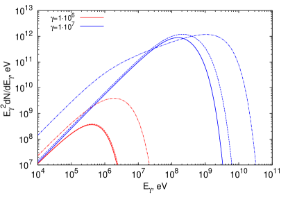
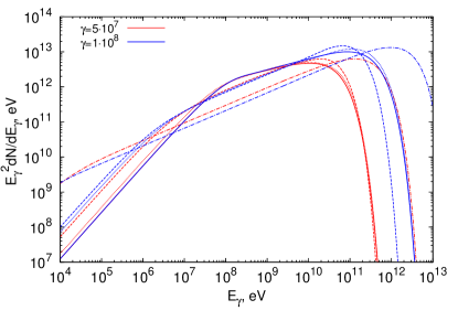
Figure 4.— Cumulative (integrated along trajectory) radiation spectra of electrons calculated for the outer gap model in the pulsar magnetosphere. The curves are obtained for the initial Lorentz factors of electrons $\gamma=10^{6}$ and $10^{7}$ (left panel), and $\gamma=5\times 10^{7}$ and $10^{8}$ (right panel). The spectra calculated in the approximation of the motion strictly along magnetic field lines are shown by solid lines. Other spectra are calculated using the exact trajectories of electrons with different initial directions relative to the magnetic field lines: along the drift trajectory (dotted lines) (not seen on the left panel because of the coincidence with solid lines), along the magnetic field line (dashed lines), and at pitch angle $\alpha=10\beta_{D}$ in the meridional plane opposite to the normal vector of magnetic field lines (dashed-dotted lines).

$\begin{array}[]{cc}\includegraphics[width=108.405pt]{fig5a}&\includegraphics[width=108.405pt]{fig5b}\\ \includegraphics[width=108.405pt]{fig5c}&\includegraphics[width=108.405pt]{fig5d}\end{array}$

Figure 5.— Time evolution of the q-parameter and the electron Lorentz factor in the outer gap model (complementary to Figure 4). The four panels correspond to the initial Lorentz factor of electrons $\gamma=10^{6},10^{7},5\times 10^{7},10^{8}$ and their initial direction along the drift trajectory.

$\begin{array}[]{cc}\includegraphics[width=108.405pt]{fig6a}&\includegraphics[width=108.405pt]{fig6b}\\ \includegraphics[width=108.405pt]{fig6c}&\includegraphics[width=108.405pt]{fig6d}\end{array}$

Figure 6.— Same as in Figure 5, but for the initial direction of electrons along the magnetic field line.

$\begin{array}[]{cc}\includegraphics[width=108.405pt]{fig7a}&\includegraphics[width=108.405pt]{fig7b}\\ \includegraphics[width=108.405pt]{fig7c}&\includegraphics[width=108.405pt]{fig7d}\end{array}$

Figure 7.— Same as in Figure 5, but for the initial direction of electrons at the angle $10\beta_{D}$.

The high-energy gamma radiation from pulsars is believed to originate from the outer gap of the pulsar magnetosphere (Cheng et al., 1986; Takata et al., 2004; Hirotani, 2008). Here we present the results of our calculations of the radiation of electrons (positrons) in the dipole magnetic field at the location of the outer gap. The position of the outer gap is placed above the last open field line. The inner boundary of the gap is at the null surface where the Goldreich–Julian charge density is zero, and the outer boundary is taken on the surface of the light cylinder. We adopt the parameters of the Crab pulsar: the radius of the star $R_{*}=10^{6}$ cm, the rotation period $P=33.5$ ms, and the magnetic field at the pole $B_{*}=10^{12}$ G. We consider a non-aligned pulsar with an angle of $45^{\circ}$ between the rotation axis and the magnetic dipole axis. The initial particle position is set at the distance $r_{\rm init}=0.5R_{lc}$ from the null surface along the last open field line, where $R_{lc}$ is the radius of the light cylinder. In numerical calculations, the particle is followed up to the intersection with the light cylinder. For parameters typical for the Crab pulsar, these conditions correspond to $\theta_{0}=51.5^{\circ}$, $R_{0}=1.2\cdot 10^{8}$ cm, $B_{0}=5.6\cdot 10^{5}$ G, and $R_{lc}=1.6\cdot 10^{8}$ cm, where $\theta_{0}$ is the polar angle relative to the magnetic dipole axis.

The energy spectra and the radiation regimes were studied for different initial directions and Lorentz factors of electrons. The resulting spectra are shown in Figure 4. The curves in Figures 5–7 demonstrate the time-evolution of the $q$-parameter (blue lines, right scale) and the Lorentz factor normalized to its initial value. These complementary plots allow us to simultaneously watch the energy loss rate and the regime of the radiation characterized by the value of the $q$-parameter. The saltatory behavior of some curves for the $q$-parameter is produced by small number of data points in the region when the energy loss rate is low.

It follows from the above discussion that the particle with a given energy radiates less intensively and produces less energetic photons when it moves along drift trajectory (i.e., in the curvature radiation regime). Indeed, locally such motion corresponds to the case when $\eta\ll 1$ or $\beta_{\perp}\ll\beta_{D}$ in Equations (50), (56), and (58). It means that $q$ oscillates around $1$ with a small amplitude of $\eta$. Then the peak of the spectrum given by Equation (58) does not shift from the position determined in curvature radiation. To check this conclusion, we set the initial direction of the particle along the drift trajectory, thus fixing the initial velocity at the angle $\beta_{D}$ from the magnetic field line toward the binormal vector. The corresponding cumulative (integrated along the trajectory) energy spectra of radiation are shown in Figure 4. The complementary plots are shown in Figure 5. We can see that, indeed, for the initial Lorentz factors $\gamma_{0}=10^{6}$ and $\gamma_{0}=10^{7}$ the curvature radiation is less energetic compared to other cases and the rates of energy losses are minimum as well (compare with corresponding curves in Figures 6 and 7).

However, the situation is different for the larger initial Lorentz factors $\gamma_{0}=5\cdot 10^{7}$ and $\gamma_{0}=10^{8}$ shown on the right panel of Figure 4. It is seen that for the initial direction along the drift trajectory, the radiation spectra extend to higher energies than in the case of the initial direction along the magnetic field. This can be explained by the very intense energy losses occurring before the particle has made the first gyration (the first oscillation of $q$-parameter). During this time interval, $q\approx 1$ for the initial direction along the drift trajectory and $q\approx 0$ for the initial direction along the magnetic field. Equations (57) and (58) show that larger values of $q$ give a more energetic radiation. Correspondingly, more energetic radiation is produced in the case of the initial direction along the drift trajectory. However, after many gyrations the energy losses in the case of the initial direction along the drift trajectory become, as expected, less intense compared to the case of the initial direction along the magnetic field line.

In Figure 4 we compare the exact calculations of radiation in the curvature regime with the results obtained under the assumption that the electron moves strictly along the magnetic field (as is routinely assumed in many papers on curvature radiation). As expected, for the relatively modest initial Lorentz factors $\gamma_{0}=10^{6}$ and $\gamma_{0}=10^{7}$, on the left panel of Figure 4, the curves for these cases merge. For larger initial Lorentz factors $\gamma_{0}=5\cdot 10^{7}$ and $\gamma_{0}=10^{8}$ the differences are not negligible, but are still small.

We call the attention of the reader to the regimes of radiation demonstrated by the curves in Figure 5. For $\gamma_{0}=10^{6}$ and $\gamma_{0}=10^{7}$, the $q$-parameter equals unity, indicating that the radiation proceeds in the curvature regime. However, this equality is not exact, as is demonstrated for $\gamma_{0}=10^{7}$ where $q$-parameter slightly oscillates around unity. These small oscillations correspond to the fine gyration around the drift trajectory. As discussed above (see Equation (55)) the presence of such fine perpendicular motions does not influence on the applicability limits.

For $\gamma_{0}=5\cdot 10^{7}$ and $\gamma_{0}=10^{8}$, the $q$-parameter has a more complex behavior. The increase at the beginning is defined mostly by the fast energy losses. The decrease is determined by the combination of several factors, such as the reduction of the magnetic field strength and the change of its curvature. The increase of $q$-parameter indicates that the radiation occurs in the synchro-curvature or the synchrotron regimes when the radiation due to curvature of the magnetic field line is less important (for $\gamma_{0}=5\cdot 10^{7}$) or simply negligible (for $\gamma_{0}=10^{8}$). According to Equation (58), the energy of the radiation maximum scales as $\sim\gamma^{3}q$. The $q$-parameter reaches the maximum when a considerable amount of energy has been lost. Therefore, in spite of large $q$, the peak of radiation shifts toward low energies and does not affect the cumulative spectrum. The interesting feature can be seen at first moments when the energy oscillates with the $q$-parameter and the minimums of $q$-parameter correspond to flatter parts of the Lorentz factor evolution curve.

The radiation spectra of electrons launched along the magnetic field line are slightly more energetic, except for $\gamma_{0}=5\cdot 10^{7}$ and $\gamma_{0}=10^{8}$ as discussed above. Initially, the radiation for $\gamma_{0}=10^{6}$ and $\gamma_{0}=10^{7}$ is in the synchro-curvature regime (see Figure 6), although for $\gamma_{0}=10^{6}$ the most of the energy is lost in the curvature regime, which occurs fast. Therefore the spectrum in this case almost coincides with the spectrum for the initial direction along the drift trajectory. For $\gamma_{0}=10^{7}$ most of the energy is lost in the synchro-curvature regime, thus the spectrum is shifted to higher energies by a factor of $q\approx 2$.

For illustration of the effect related to initial pitch angles larger than $\beta_{D}$, we show the case of the initial direction deflected at the angle $10\beta_{D}$ from the magnetic field line toward the direction opposite the normal vector. The corresponding spectra indicated in Figure 4 by dashed-dotted lines are shifted toward higher energies. Although the $q$-parameter (Figure 7) reaches large values, most of the energy is lost at initial stages at $q\approx 10$. Thus the spectra are shifted by $q\approx 10$ compared to the curvature radiation spectra.

We should note that the energy spectra of radiation produced in all regimes at highest energies contain an exponential cut-off similar to the spectrum of the small-angle synchrotron radiation. However, since the radiation spectrum is very sensitive to the pitch-angle, a population of electrons with similar energies but different angles can result in a superposition spectrum with a less abrupt cut-off. The condition for the realization of such a spectrum is that the distribution of electrons over the angles around the drift trajectory should be wider than $\beta_{D}$.

5.2. Polar Cap

In the polar cap model the electron radiates in the region located close to the surface of the neutron star, where the magnetic field is much stronger than in the outer gap model, approaching to $B\approx 10^{12}$ G. This results in much faster damping of the perpendicular component of motion. The very small drift velocity $\beta_{D}$ implies that the drift trajectory and the magnetic field line almost coincide, thus even a small deflection from the magnetic field line produces radiation that is quite different from the curvature radiation. However, the transition to the curvature radiation regime occurs very fast. In the curvature regime electrons radiate more energetic photons than in the outer gap model because of the stronger curvature of the field lines. The curvature of the dipole field lines behaves like $\sim\sin\theta/r$, and with the decrease of the radius by two orders of magnitude and the decrease of the polar angle by an order of magnitude ($\theta_{0}\sim 1^{\circ}$), the curvature is larger by an order of magnitude compared to the case of outer gap model. Correspondingly, the maximum energy of the curvature radiation in the polar cap is an order of magnitude higher than in the outer gap.

The energy spectra of radiation calculated for the polar cap model are shown in Figure 8. The complementary plots for the evolution of the $q$-parameter and the electron Lorentz factor are presented in Figures 9-11. The initial position of the particle is $R_{0}=10^{6}$ cm, and $\theta_{0}=3^{\circ}$. The spectra indicated by solid lines correspond to the case when the initial direction of the particle is along the magnetic field line. In this case the radiation is in the curvature regime. Initially, the radiation shortly proceeds in the synchro-curvature regime, but abruptly turns to the regime with fast oscillations around $q\approx 1$ caused by fine gyrations (Figure 9).

In the case of an initial pitch angle $\alpha_{0}=1/\gamma_{0}$ the abrupt change of regimes leads to an interesting feature in the cumulative spectra (dashed lines). Because of small changes of the energy and fast changes of the $q$-parameter, an energy spectrum is formed consisting of two peaks. The peak at higher energies is produced in the synchrotron regime ($q\gg 1$, see Figure 10), while the lower energy peak is due to radiation in the curvature regime. The double-peak structure disappears for large initial pitch angles. For example, for the pitch angle $100/\gamma_{0}$ the transition to the curvature regime is very fast and the electron enters into this regime with dramatically reduced Lorentz factor. Thus the peak of the curvature radiation is not only shifted to smaller energies, but also too weak to be seen in the cumulative spectrum.

In very strong magnetic fields, namely when the parameter $\chi=B\gamma\sin\alpha/B_{cr}\geq 1$, the radiation is produced in the quantum regime. Let’s assume that the initial pitch angle is inversely proportional to the initial Lorentz factor, $\alpha_{0}=a/\gamma_{0}$. This makes the condition of radiation in the quantum regime independent of $\gamma_{0}$:

$$\chi=\frac{B}{B_{cr}}\gamma\sin{\alpha_{0}}=\frac{1\cdot 10^{12}G}{2.94\cdot 10^{13}G}a\approx 3.4\cdot 10^{-2}a.$$ (85)

Thus, at the initial pitch angle with $a>30$, the electrons radiate in the quantum regime. Dashed-dotted lines in Figure 8 present radiation spectra for the initial pitch-angles $\alpha_{0}=100/\gamma_{0}$. Note that in the quantum regime almost the entire energy of the parent electron is transferred to the radiated photon. Therefore we should expect an abrupt cutoff in the radiation spectra. This effect is clearly seen in Figure 8 (dot-dashed curves corresponding to the initial pitch angle $\alpha_{0}=100/\gamma_{0}$). The gamma-rays produced in the quantum regime are sufficiently energetic to be absorbed in the magnetic field through the $e^{+}e^{-}$ pair production. This leads to the development of an electromagnetic cascade in the magnetic field. The spectrum of cascade gamma-rays that escape the pulsar magnetosphere will be quite different from the spectra shown in Figure 8.

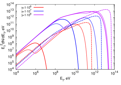
Figure 8.— Cumulative (integrated along trajectory) radiation spectra of electrons calculated for the polar cap model in the pulsar magnetosphere. The curves are obtained for different initial Lorentz factors of electrons $\gamma=10^{6},10^{7},10^{8}$, and for different initial directions relative to the magnetic field lines: along the magnetic field line (solid lines), and for two pitch angles $1/\gamma_{0}$ (dashed lines) and $100/\gamma_{0}$ (dot-dashed lines).

$\begin{array}[]{cc}\includegraphics[width=108.405pt]{fig9a}&\includegraphics[width=108.405pt]{fig9b}\end{array}$

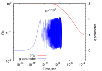
Figure 9.— Time evolution of the $q$-parameter and the electron Lorentz factor in the outer gap model (complementary to Figure 8). The three panels correspond to the initial Lorentz factor of electrons $\gamma=10^{6},10^{7},10^{8}$ and their initial direction along the magnetic field line.

$\begin{array}[]{cc}\includegraphics[width=108.405pt]{fig10a}&\includegraphics[width=108.405pt]{fig10b}\end{array}$

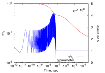
Figure 10.— Same as in Figure 9, but for the initial direction of electrons at the pitch angle $1/\gamma_{0}$.

$\begin{array}[]{cc}\includegraphics[width=108.405pt]{fig11a}&\includegraphics[width=108.405pt]{fig11b}\end{array}$

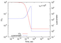
Figure 11.— Same as in Figure 9, but for the initial direction of electrons at the pitch angle $100/\gamma_{0}$.

6. Motion and radiation in electric and magnetic fields

To study a more realistic picture of the radiation, one should consistently determine the initial pitch angle. This can be done if the acceleration of the particle is considered. First we consider the motion of a charged particle in the crossed homogeneous electric and magnetic fields. If the fields are not perpendicular to each other, one can always find a reference frame in which they are parallel. In this reference frame the particle completely loses the momentum perpendicular to the common direction of the electric and magnetic fields. At the same time, the electric field infinitely accelerates the particle. Eventually the particle accelerates along the common direction of the electric and magnetic fields. In an arbitrary reference frame the particle is accelerated along a rectilinear trajectory. However, the direction of the motion is

$$\boldsymbol{\beta}=\frac{1}{Q}\mathbfcal{E}\times\boldsymbol{B}\pm\left(\frac{\sqrt{Q-\boldsymbol{B}^{2}}}{Q}\mathbfcal{E}+\frac{\sqrt{Q-\mathbfcal{E}^{2}}}{Q}\boldsymbol{B}\right),$$ (86)

where

$$Q=\frac{\mathbfcal{E}^{2}+\boldsymbol{B}^{2}}{2}+\sqrt{\left(\frac{\mathbfcal{E}^{2}-\boldsymbol{B}^{2}}{2}\right)^{2}+(\mathbfcal{E}\boldsymbol{B})^{2}},$$ (87)

and $+$ and $-$ signs correspond to positively and negatively charged particles, respectively. Then the pitch angle can be expressed as

$$\sin\alpha=\frac{\sigma\sin\theta}{\sqrt{\frac{1}{2}\left(\sqrt{(1+\sigma^{2})^{2}-4\sigma^{2}\sin^{2}\theta}+(1+\sigma^{2})\right)}},$$ (88)

where $\sigma=\mathscr{E}/B$ is the ratio of the electric and magnetic fields, and $\theta$ is the angle between them. Assuming that the electric field is typically smaller than the magnetic field, we obtain

$$\alpha\approx\beta_{E}=\sigma\sin\theta\ll 1$$ (89)

which implies that the pitch angle equals the electric drift velocity (in units of the speed of light). Thus, in the crossed homogeneous electric and magnetic fields, the asymptotic motion of the particle after damping of gyration is a constant acceleration along the rectilinear trajectory. The direction of the trajectory constitutes the angle $\beta_{E}$ with the direction of the magnetic field. Note that due to this acceleration the particle radiates. However, the energy losses do not depend on the Lorentz factor and are negligibly small compared to the energy losses during the particle motion along the curved trajectory.

In the curved electric and magnetic fields the acceleration of the particle is restricted by the energy losses due to the curved trajectory. Once the characteristic times of the acceleration and radiation become equal, the particle moves along a drift trajectory determined by the electric and magnetic fields. During radiation the particle changes its direction of motion. At the same time it is accelerated by the electric field in the direction determined by Equation (86). As in the case of crossed homogeneous electric and magnetic fields, the component of the momentum perpendicular to the drift trajectory, which is responsible for the gyration of the particle, is damped due to radiation. Thus, in the equilibrium between acceleration and radiation, the particle moves along drift trajectory practically without gyration with the pitch angle $\beta_{E}$. If the electric or magnetic field changes slowly along trajectory, it gradually adjusts itself to the equilibrium state of the drift trajectory. However, if fields vary fast, it can lead to a strong radiation until the particle gets a new equilibrium drift trajectory. Such conditions might appear when the particle escapes the acceleration gap and the field-aligned (along magnetic field lines) electric field is screened.

Further we study the radiation of the particle inside and outside the outer gap. We check how the character of the radiation changes depending on the variation of the electric field. Specifically, we consider the case of screening the fieldaligned electric field when it decreases exponentially from the border of the outer gap. The geometry of the model is presented in Figure 12. As before, the angle between the rotation and dipole axes is $45^{\circ}$. The strength of the magnetic field at the pole of the star is $B_{*}=10^{12}$ G. The period of rotation of the star is $P=33$ msec. The configuration of the electric and magnetic fields is given by the approximation of Deutsch (1955) for the fields in the vacuum in the vicinity of a rotating star (equations (18) and (19) in Deutsch (1955)). The magnetic field in this approximation is just a dipole magnetic field. The outer gap is located between the null surface and the last open field line. We set the border of the gap at $x_{b}=0.7R_{lc}$ from the rotation axis (see the black vertical line in Figure 12), where $R_{lc}$ is the radius of the light cylinder. In our calculations we assume that the field-aligned electric field is screened starting from $x_{b}$ according to the exponential decay:

$$\mathscr{E}_{\parallel}=\mathscr{E}_{0\parallel}e^{-\left(\frac{x-x_{b}}{W}\right)^{2}},$$ (90)

where $\mathscr{E}_{0\parallel}$ is the original component of the electric field parallel to the magnetic field (as it would change without screening). Note that the perpendicular component stays unmodified. Changing the width of the screening $W$, we can explore different models for the variation of the electric field. The three cases that we investigate, $W=10^{-3}R_{lc}$, $10^{-2}R_{lc}$, and $10^{-1}R_{lc}$, cover a large range of values of this parameter. The calculation of the trajectory starts from the null surface at a distance $x=0.4R_{lc}$ from the rotation axis, with initial Lorentz factor $\gamma_{0}=100$ and velocity directed along magnetic field line.

Together with calculations using the exact equations of motion given by Equation (A1), we performed the calculations in the drift approximation presented by Equation (A3). The approach of the drift approximation has been used in the work Kalapotharakos et al. (2012) to calculate the light curves for the different models of the magnetosphere. Here it is important for us to investigate how well this approach reproduces the radiation spectra. Apart from the described configuration of the electric field, we carried out the calculations for more simple electric fields when their strength is proportional to the strength of the magnetic field and their direction is always at a constant angle to the direction of the magnetic field at a given point. The results for a broad range of values for the angles and strength ratios have shown a very good agreement between the exact and approximate approaches. We do not show them because the case of the configuration considered here is quite representative. The explanation of the good agreement between radiation spectra calculated in exact and approximate approaches is that in both cases the curvatures of the trajectories are very close. As discussed previously, in the equilibrium between the acceleration and radiation the particle basically moves along drift trajectory, which is assumed a priori in the drift approximation.

The projection of the trajectories on the XZ plane calculated in both approaches are presented in the Figure 12. The trajectories outside the gap are shown for the case of the slow variation of the electric field $W=10^{-1}R_{lc}$ when the scale of change is of the same order as the scale of the gap. Before we discuss the influence of screening on the particle motion and radiation, let us consider phenomena in the gap.

Aside from the initial moments when the particle is accelerated fast, it moves along equilibrium drift trajectory. In the equilibrium regime when the acceleration by electric field is balanced by energy losses of radiation, the position of the maximum of the energy distribution $\epsilon_{*}$ is given by (see Appendix C):

$$\epsilon_{*}=\left(\frac{3}{2}\right)^{\frac{7}{4}}\left(\frac{\sigma\cos\theta B}{e}\right)^{\frac{3}{4}}c\hbar\sqrt{r_{0}\left(1+\sigma^{2}\sin^{2}\theta\right)},$$ (91)

where $r_{0}$ is the curvature of the magnetic field line, and $e$ is the elementary charge. The equation is valid for $\sigma<1$. Note that in the derivation of Equation (91), the energy losses were taken in the form given by Equation (48). For comparison, if the cooling of electrons is dominated by synchrotron losses, we obtain the classical limit for maximum energy of radiation:

$$\epsilon_{syn}=\frac{9}{4}\frac{mc^{2}}{\alpha_{f}}\sigma\cos\theta,$$ (92)

where $\alpha_{f}=e^{2}/\hbar c\approx 1/137$ is the fine-structure constant. The comparison of Equations (91) and (92) shows that the former depends on the strength and the curvature of the magnetic field, whereas in Equation (92) the magnetic field only enters through the ratio $\sigma\cos\theta=\mathscr{E}_{\parallel}/B$. In the case of a strong electric field ($\sigma=1$, $\theta=0^{\circ}$) and the dominance of energy losses by synchrotron radiation, the maximum energy of radiation is restricted by $\epsilon_{syn}\approx 160$ MeV. If the energy losses of electrons occur in the curvature or synchro-curvature regimes, the position of the maximum moves to higher energies. For example, for parameters used in our numerical calculations, the radiation maximum can be as high as $30$ GeV (see Figure 13). Thus, less intense energy losses of the curvature radiation lead to more energetic radiation. Remarkably, with an increase of curvature radius $r_{0}$ the radiation becomes more energetic.

For comparison of the drift approximation and the exact calculation, it is convenient, as above, to introduce the $q$-parameter. However, in cases when only the magnetic field presents, the $q$-parameter has been determined by Equation (56) as ratio of the curvature of the real trajectory and the curvature of the magnetic field lines. Now, when we compare the real trajectory and the electric drift trajectory, we determine $q$-parameter to be $q=R_{E}/R_{c}$, where $R_{E}$ and $R_{c}$ are the curvature radii of the electric drift and the real trajectory, respectively. Then the characteristic frequencies of the radiation in both cases are related as $\epsilon_{c}=q\epsilon_{E}$. One can see from the right panel of Figure 13 that in the gap (green lines) the Lorentz factors are close and the $q$-parameter is practically unity. The small difference in the Lorentz factors produces a small difference in the radiated spectra presented in the left panel of Figure 13 by red and green lines. This difference could be explained by the fact that the trajectories in the drift approximation and the exact calculation are not identical, as can be seen from Figure 12, and the particle experiences slightly different magnetic and electric fields.

When the particle escapes the outer gap it experiences the decrease of the field-aligned electric field. We explore how this drop in strength influences the radiation of the particle depending on the intensity (gradient) of the drop. The relevant Lorentz factors and $q$-parameter are shown in the right panel of Figure 13. In the case of the slow decrease of the field-aligned electric field with $W=10^{-1}R_{lc}$ (pink lines), the $q$-parameter is unity and the Lorentz factors for approximate and exact calculations follow each other, gradually decreasing. In this case the radiation spectra are close. For a more quickly decreasing electric field ($W=10^{-2}R_{lc}$, blue lines) the $q$-parameter oscillates around unity, and there is a slight divergence between the Lorentz factors calculated in different approaches (especially close to the gap border), but the resulting spectra do not differ significantly. A different situation occurs when the field-aligned electric field drops very fast with screening width $W=10^{-3}R_{lc}$ (brown lines). The $q$-parameter increases quickly on several orders of magnitude. At the same time, the Lorentz factor in the exact calculation drops, whereas in the drift approximation it continues to change gradually. This produces different spectra calculated in two approaches. The exact calculation gives more energetic radiated photons compared to the drift approximation (solid lines in the left panel of Figure 13). Thus, in the case of fast screening, the drift approximation does not work.

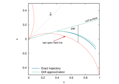
Figure 12.— Projection on the XZ plane of the trajectories of the electrons emitting the spectra in Figure 13. The initial Lorentz factor is $\gamma_{0}=100$. The particles begin to be accelerated from the null surface at $x=0.4R_{lc}$. The distances of axes in units of the light cylinder. The border of the gap is at $x=0.7R_{lc}$. The trajectories outside the gap are presented for the case of exponential screening with the width $W=0.1R_{lc}$.

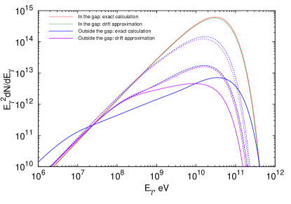
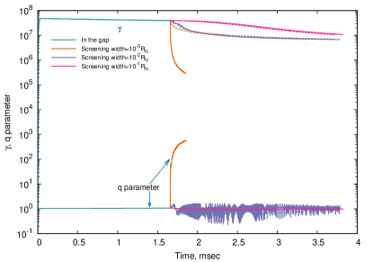
Figure 13.— Left panel: cumulative radiation spectra of electrons accelerated in the gap (red and green lines), and radiation spectra of electrons outside the gap (blue and purple lines) with screening width $W=10^{-1}R_{lc}$ (dotted lines), $W=10^{-2}R_{lc}$ (dashed lines), $W=10^{-3}R_{lc}$ (solid lines) obtained in the exact numerical calculations (blue lines) and using the drift approximation (purple lines). Right panel: evolution of the Lorentz factor and $q$-parameter with time.

7. Discussion

In curved magnetic fields the particle trajectories acquire a complex structure when the curvature of the averaged drift trajectory is superimposed on the regular curvature of its gyration. The interplay of the two components produces a variable curvature of the particle trajectory. This results in the variability of radiation where the intensity and the spectrum are changed with the period of the particle gyration. The variability becomes pronounced during the transition from the synchrotron to the curvature radiation regime when the two components of the curvature of the trajectory become comparable. During this transition the radiation cannot be described by synchrotron or curvature modes, but rather by their combination – synchro-curvature radiation.

Because of the fast variability, only the averaged spectrum of radiation can be observed. The spectrum averaged over the period of gyration is described by Equation (59) and depends on two parameters. At small or large values of the $\eta$ parameter, the spectrum coincides with the standard form of the synchrotron spectrum. It is important to note that the radiation could not be reduced to the formalism of the synchrotron radiation by introducing a single effective curvature radius. Indeed, the intensity of radiation averaged over the period of gyration is given by Equation (50). It can be represented in the standard form of Equation (48), if we introduce an effective curvature radius $R_{\rm eff}=r_{0}/\sqrt{1+\eta^{2}}$. However, if we want to have a standard exponential term e-x in an explicit form (as in the case of the synchrotron or curvature radiation) in the asymptotic presentation of the spectrum given by Equation (64), the effective curvature radius should be defined differently, namely $R_{\rm eff}=r_{0}/(1+\eta)$.

The conditions for the realization of one or another regime are determined by the relation between the drift velocity $\beta_{D}$ and the velocity perpendicular to the drift trajectory $\beta_{\perp}$. The general conditions of the applicability of synchro-curvature radiation are also described in terms of $\beta_{D}$ and $\beta_{\perp}$ by Equation (55). In the model case of a magnetic field of constant curvature and without energy losses, $\beta_{\perp}$ is a free parameter. If $\beta_{\perp}=0$, the particle can move along a drift trajectory without gyration. This case is associated with the pure curvature radiation, which occurs solely due to curvature of magnetic field line. In the strong magnetic field, the drift trajectory is close to the field lines, so the substitution of the curvature of the field lines instead of the curvature of the drift trajectory is an acceptable approximation. In particular, in the radiation formulas we have neglected this difference assuming that the condition given by Equation (8) is fulfilled.

The spectrum of radiation becomes quite sensitive to the pitch angles if $\beta_{\perp}\geq\beta_{D}$, with a shift of the maximum to higher energies roughly as $1+\eta$. Therefore any angular distribution of particles wider than $\beta_{D}$ produces a superposition spectrum with a high-energy cutoff that falls down slower than the standard exponential cutoff of the synchrotron or curvature radiation. Taking into account that in a strong magnetic field $\beta_{D}$ is very small, even in the case of a very narrow angular distribution, the radiation spectrum could differ significantly from the unidirectional beam. This is demonstrated in Figures 2 and 3, where the radiation spectra is averaged over the pitch-angles of particles, assuming that Gaussian type and uniform angular distributions of particles are presented. For the Gaussian type angular distribution, the spectral flux density can be presented in a simple analytical form by Equation (3), which provides good accuracy at $x\gtrsim 0.5$. As seen from Figure 3, spectra becomes harder compared to the curvature radiation ($\zeta=0$). It could also be noted that different angular distributions with the equal width give similar spectra.

This interesting feature may be a key for the interpretation of the recent observations of pulsars by Fermi LAT that indicate that the energy spectra of some pulsars, in particular the Crab pulsar (Buehler et al., 2012), in the cutoff region are significantly harder than $e^{-x}$, as predicted by the curvature radiation models. The energy spectrum of the pulsed emission of the Crab reported in (Buehler et al., 2012) can be readily described by Equation (73) assuming $\zeta=1$ and a quite reasonable value for the ratio $\gamma^{3}/r_{0}\simeq 10^{13}\;{\rm cm}^{-1}$. It should be noted that the form of the high-energy cutoff does not depend on energy losses because it is produced by the most energetic particles at the first moments of radiation before they lose their energy. The angular distribution with enough broad angular width could appear when the particles accelerated along different field lines enter the region of the screened electric field.

The results of the simplified analytical approach are confirmed by detailed numerical calculations. More importantly, the numerical calculations allow a rather general treatment of the problem extending to the case when the energy losses of electrons are taken into account. We studied the radiation for the parameters typical for the polar cap and outer gap models of the pulsar magnetosphere following the evolution of the radiation of electrons with different initial pitch angles in a dipole magnetic field. As expected, the least energetic radiation is produced by electrons with an initial angle along the drift trajectory. The particle radiates in the synchro-curvature regime if the initial pitch angle is of the order of $\beta_{D}$, in particular, if the initial direction is along the magnetic field line. The spectra are substantially more energetic when the initial pitch angle exceeds $\beta_{D}$. For typical parameters of the polar cap model $\beta_{D}=2.2\cdot 10^{-9}(\gamma/10^{8})$, so even a slight deflection from the field line results in the production of synchrotron radiation in the quantum regime. Moreover, this creates the interesting feature of a double peaked spectrum (see Figure 8) if the initial pitch angle is $1/\gamma_{0}$.

In the context of the quantum synchrotron radiation, we should note the following circumstance. The photons are produced in a quantum regime when the pitch angle of the charged particle is sufficiently large. The direction of the produced photons is basically along the direction of the charged particle. Thus, the photons are produced at large angles to the magnetic field. The fact that the photons have approximately the energy of the parent charged particles implies that the parameter $\chi=B\gamma\sin\alpha/B_{cr}\geq 1$, thus the photon should produce an electron-positron pair and initiate an electromagnetic cascade. In this case, the cascade starts earlier than in the case of gamma-rays produced along the magnetic field lines.

Due to the variation of the strength and the curvature of the dipole magnetic field, the change of radiation regimes is a quite complex process as can be seen from the variation of the $q$-parameter in Figures 5-7. The transition to the curvature regime occurs with different rates for the polar cap and the outer gap environment. Whereas in the polar cap the particle makes a transition to the curvature regime very fast (see Figure 10), the particle in the outer gap can radiate in the synchro-curvature regime most of the time while passing the gap (see the second panel of Figure 6). Although in the polar cap the synchrotron regime only lasts briefly, the particle loses most of its energy during this regime. Namely, if the initial pitch angle is $a/\gamma_{0}$ ($a\geq 1$), the initial Lorentz factor on the drift trajectory is about $\gamma_{0}/a$. Since the typical Lorentz factor is $\gamma\approx 10^{7}$, the huge energy losses could be caused by a very small pitch angle.

The treatment of pitch angles is not self-consistent without the consideration of particle acceleration. To study this question we examined the model of the acceleration in the electric and magnetic fields of the vacuum-retarded dipole (Deutsch, 1955), as well as other simple models of the electric field. The calculations show that the particle basically moves along the drift trajectory jointly defined by the electric and magnetic fields. Therefore the approach of drift approximation applied in the work of Kalapotharakos et al. (2012) gives results that are similar to those obtained in the exact consideration. The difference could arise when the particle escapes the acceleration gap experiencing the decrease of the field-aligned electric field. It has been shown that in the case of the fast screening of the electric field the particle can start to radiate more intensely. As a result, the particle radiates more energetic photons than is predicted by the drift approximation. In general, the drift approximation and the curvature radiation can only be applied to the equilibrium situations when the model parameters change slowly.

Appendix A Motion of a charged particle in electric and magnetic fields

The motion of an ultrarelativistic charged particle in the electric ($\mathbfcal{E}$) and magnetic ($\boldsymbol{B}$) fields is described by the system of equations (Landau & Lifshitz, 1975):

$$\frac{d\boldsymbol{r}}{dt}=c\boldsymbol{\beta},$$ (A1)

$$\frac{d\boldsymbol{\beta}}{dt}=\frac{e}{mc\gamma}(\mathbfcal{E}-(\boldsymbol{\beta}\mathbfcal{E})\boldsymbol{\beta}+\boldsymbol{\beta}\times\boldsymbol{B}),$$

$$\frac{d\gamma}{dt}=\frac{e}{mc}(\boldsymbol{\beta}\mathbfcal{E})-\frac{2e^{2}}{3mc}\frac{\gamma^{4}}{R_{c}^{2}},$$

where the curvature radius is expressed as

$$\frac{1}{R_{c}}=\left|\frac{d\boldsymbol{\beta}}{cdt}\right|=\frac{e}{mc^{2}\gamma}\sqrt{(\mathbfcal{E}+\boldsymbol{\beta}\times\boldsymbol{B})^{2}-(\boldsymbol{\beta}\mathbfcal{E})^{2}}.$$ (A2)

The motion of an ultrarelativistic charged particle in the drift approximation is determined by the following system of equations:

$$\frac{d\boldsymbol{r}}{dt}=c\boldsymbol{\beta},$$ (A3)

$$\frac{d\gamma}{dt}=\frac{e}{mc}(\boldsymbol{\beta}\mathbfcal{E})-\frac{2e^{2}}{3mc}\frac{\gamma^{4}}{R_{c}^{2}},$$

where

$$\boldsymbol{\beta}=\frac{\mathbfcal{E}\times\boldsymbol{B}}{B^{2}}+f\frac{\boldsymbol{B}}{B},$$ (A4)

and $f$ is defined from the condition that $\left|\boldsymbol{\beta}\right|=1$

$$f=\sqrt{1-\left(\frac{\mathbfcal{E}\times\boldsymbol{B}}{B^{2}}\right)^{2}}.$$ (A5)

Then the curvature of the trajectory is

$$\frac{1}{R_{c}}=\left|\boldsymbol{K}\right|=\left|(\boldsymbol{\beta}\nabla)\boldsymbol{\beta}\right|.$$ (A6)

Note that the differential equations that describe the evolution of Lorentz factor have the same form in both approaches. The difference is in the determination of the curvature radius.

Appendix B Energy losses in the quantum regime

In a strong magnetic field, the ultrarelativistic electrons can radiate in the quantum regime, provided that

$$\chi=\frac{B}{B_{cr}}\gamma\sin\alpha\gtrsim 1,$$ (B1)

where $B_{cr}=\frac{2m^{2}c^{3}}{3e\hbar}\approx 2.94\cdot 10^{13}$ G. In the presence of electric field, $B\sin\alpha=|(\boldsymbol{\beta}\times\boldsymbol{B})|$ should be substituted by $\sqrt{(\mathbfcal{E}+\boldsymbol{\beta}\times\boldsymbol{B})^{2}-(\boldsymbol{\beta}\mathbfcal{E})^{2}}$. The energy loss rate can be written in the form (Bayer et al., 1973; Berestetskii et al., 1982)

$$\left|\frac{dE}{dt}\right|=\frac{e^{2}m^{2}c^{3}}{\sqrt{3}\pi\hbar^{2}}\overline{H}(\chi)\,,$$ (B2)

where

$$\overline{H}(\chi)=\int_{0}^{1}H(\tau,\chi)d\tau\ ,$$ (B3)

and

$$H(\tau,\chi)=\chi\left[(1-\tau)F(x)+x\tau^{2}K_{2/3}(x)\right],\quad x=\frac{\tau}{\chi(1-\tau)},$$ (B4)

where $K_{2/3}(x)$ is the modified Bessel function of the order $2/3$, $F(x)$ is the emissivity function of the synchrotron radiation (see Equation 54), $\tau=\epsilon/E$, where $\epsilon$ is the energy of the radiated photon, $E$ is the energy of the radiating particle.

For calculations it is convenient to express $\overline{H}(\chi)$ in Equation (B2) in a simple approximate analytical form. Using asymptotics of this function

$$\begin{aligned} &\overline{H}(\chi)\approx{\frac{8\pi\sqrt{3}}{27}}{\chi}^{2},\quad\chi\ll 1,\\ &\overline{H}(\chi)\approx{\frac{32\pi\sqrt{3}}{243}}{2}^{2/3}\Gamma\!\left(\frac{2}{3}\right)\chi^{2/3},\quad\chi\gg 1.\end{aligned}$$ (B5)

we suggest the following approximation

$$\overline{H}(\chi)\approx\frac{8\pi\sqrt{3}}{27}\frac{\chi^{2}}{\left({\displaystyle 1+\frac{3}{4}\frac{(2\chi)^{2/3}}{\sqrt{\Gamma\!\left(\frac{2}{3}\right)}}}\right)^{2}}\times\left(1+\frac{0.52\sqrt{\chi}(1+3\sqrt{\chi}-3.2\chi)}{1+0.3\sqrt{\chi}+17\chi+11\chi^{2}}\right)$$ (B6)

The first part of Equation (B6) (before the sign $\times$) gives right asymptotics at $\chi\ll 1$ and $\chi\gg 1$ and provide an accuracy better than $10\%$ for other values of $\chi$, whereas the last term in the brackets improves the accuracy down to $0.1\%$ for any $\chi$.

The spectrum of radiation in the quantum regime is described by the function that can be written as

$$F_{q}(x,\tau) =(1-\tau)F(x)+\tau^{2}xK_{2/3}(x),\quad x =\frac{\tau}{1-\tau}\frac{E}{\epsilon_{c}},$$ (B7)

where $\epsilon_{c}=\frac{3e\hbar B\sin\alpha}{2mc}\gamma^{2}$ is the characteristic energy of the emitted photon. To use this function in Equation (57), the variable $\epsilon_{c}$ should be replaced by $\hbar\omega_{*}$. An analytical approximation of this function can be obtained using the approximation for emissivity function of the synchrotron radiation (Aharonian et al., 2010)

$$F(x)\approx 2.15x^{1/3}(1+3.06x)^{1/6}\frac{1+0.884x^{2/3}+0.471x^{4/3}}{1+1.64x^{2/3}+0.974x^{4/3}}e^{-x},$$ (B8)

and

$$xK_{2/3}(x)\approx 1.075x^{1/3}(1+3.72x)^{1/6}\frac{1+1.58x^{2/3}+3.97x^{4/3}}{1+1.53x^{2/3}+4.25x^{4/3}}e^{-x}.$$ (B9)

Both approximations provide an accuracy better than $0.2\%$ for any value of the argument $x$.

Appendix C Maximum of the curvature radiation spectrum

The maximum energy of the electron determined from the competition between the acceleration and the energy losses, is found from the condition $t_{acc}=t_{loss}$, where

$$t_{loss}=\frac{E}{|dE/dt|_{loss}}=\frac{3mcR_{c}^{2}}{2e^{2}\gamma^{3}},$$ (C1)

and

$$t_{acc}=\frac{E}{|dE/dt|_{acc}}=\frac{E}{ce\sigma\cos\theta B}=\frac{mc\gamma}{e\sigma\cos\theta B}.$$ (C2)

Note that the acceleration rate is defined as $|dE/dt|_{acc}=ce\mathscr{E}\cos\theta$, where $\mathscr{E}$ is electric field, $\sigma=\mathscr{E}/B$ is the ratio of the electric and magnetic fields, and $\theta$ is the angle between them. From $t_{loss}=t_{acc}$ we obtain Lorentz factor of the electron:

$$\gamma_{eq}=\left(\frac{3\sigma\cos\theta BR_{c}^{2}}{2e}\right)^{\frac{1}{4}}.$$ (C3)

Substituting this equation into the expression for the characteristic energy of radiation given by Equation (53) we find

$$\epsilon_{*}=\left(\frac{3}{2}\right)^{\frac{7}{4}}\left(\frac{\sigma\cos\theta B}{e}\right)^{\frac{3}{4}}c\hbar\sqrt{R_{c}}.$$ (C4)

Finally, taking into account that the curvature of the drift trajectory is $R_{c}=r_{0}(1+\beta_{E}^{2})$, where $\beta_{E}=\sin\alpha$ is the drift velocity due to the electrical drift, and $\alpha$ is the pitch angle given by Equation (89), we obtain

$$\epsilon_{*}=\left(\frac{3}{2}\right)^{\frac{7}{4}}\left(\frac{\sigma\cos\theta B}{e}\right)^{\frac{3}{4}}c\hbar\sqrt{r_{0}\left(1+\sigma^{2}\sin^{2}\theta\right)},$$ (C5)

where $r_{0}$ is the curvature of the magnetic field line.

References

- Aharonian et al. (2010) Aharonian, F. A., Kelner, S. R., & Prosekin, A. Y., 2010. Phys. Rev. D, vol. 82, 4, 043002
- Bayer et al. (1973) Bayer, V. N., Katkov, V. M., & Fadin, V. S., 1973. Radiation of Relativistic Electrons (Atomizdat, Moscow)
- Berestetskii et al. (1982) Berestetskii, V. B., Lifshitz, E. M., & Pitaevskii, L. P., 1982. Quantum Electrodynamics (Butterworth-Heinemann, Oxford)
- Buehler et al. (2012) Buehler, R., Scargle, J. D., Blandford, R. D. et al., 2012. ApJ, vol. 749, 26
- Cheng et al. (1986) Cheng, K. S., Ho, C., & Ruderman, M., 1986. ApJ, vol. 300, 500
- Cheng & Zhang (1996) Cheng, K. S. & Zhang, J. L., 1996. ApJ, vol. 463, 271
- Deutsch (1955) Deutsch, A. J., 1955. Annales d’Astrophysique, vol. 18, 1
- Epstein (1973) Epstein, R. I., 1973. ApJ, vol. 183, 593
- Harko & Cheng (2002) Harko, T. & Cheng, K. S., 2002. MNRAS, vol. 335, 99
- Hirotani (2008) Hirotani, K., 2008. ApJ, vol. 688, L25
- Kalapotharakos et al. (2012) Kalapotharakos, C., Harding, A. K., Kazanas, D. et al., 2012. ApJ, vol. 754, L1
- Landau & Lifshitz (1975) Landau, L. D. & Lifshitz, E. M., 1975. The Classical Theory of Fields (Butterworth-Heinemann, Oxford)
- Schwinger (1949) Schwinger, J., 1949. Phys. Rev., vol. 75, 1912
- Sobolev (2006) Sobolev, Y. M., 2006. Problems of Atomic Science and Technology, vol. 5, 157
- Takata et al. (2004) Takata, J., Shibata, S., & Hirotani, K., 2004. MNRAS, vol. 354, 1120