Listening to features

This work explores nonparametric methods which aim at synthesizing audio from low-dimensionnal acoustic features typically used in MIR frameworks. Several issues prevent this task to be straightforwardly achieved. Such features are designed for analysis and not for synthesis, thus favoring high-level description over easily inverted acoustic representation. Whereas some previous studies already considered the problem of synthesizing audio from features such as Mel-Frequency Cepstral Coefficients, they mainly relied on the explicit formula used to compute those features in order to inverse them. Here, we instead adopt a simple blind approach, where arbitrary sets of features can be used during synthesis and where reconstruction is exemplar-based. After testing the approach on a speech synthesis from well known features problem, we apply it to the more complex task of inverting songs from the Million Song Dataset. What makes this task harder is twofold. First, that features are irregularly spaced in the temporal domain according to an onset-based segmentation. Second the exact method used to compute these features is unknown, although the features for new audio can be computed using their API as a black-box. In this paper, we detail these difficulties and present a framework to nonetheless attempting such synthesis by concatenating audio samples from a training dataset, whose features have been computed beforehand. Samples are selected at the segment level, in the feature space with a simple nearest neighbor search. Additionnal constraints can then be defined to enhance the synthesis pertinence. Preliminary experiments are presented using RWC and GTZAN audio datasets to synthesize tracks from the Million Song Dataset.

Chapter 0 Introduction

1 From audio to features

Audio features [1, 2] are mid-level characteristics such as pitch, Mel-Frequency Cepstral Coefficients (MFCC), loudness etc., which are computed from audio signals and whose purpose is to serve as meaningful observations in audio machine learning tasks. For example, they are fundamental in fingerprinting systems, that consist in recognizing a whole musical song from a database, based on the distorted measurement of an excerpt of a few seconds only [3, 4, 5, 6]. The use of features such as MFCC is also paramount in many classical automatic speech transcription systems [7] and, more generally, in most audio information retrieval studies.

1 … and backwards ?

Audio features are most commonly used in an analysis setup, where they are practical proxies that yield meaningful representations for machine learning algorithms to work on. For synthesis purposes, only a limited number of them, such as MFCC along with pitch and loudness information, are commonly used to control parametric speech synthesizers [8, 9, 10, 11, 12]. However, these synthesis methods typically exploit the explicit knowledge of how the features are computed in order to inverse them. In the case of MFCC, for example, it is straightforward to relate the coefficients back to the spectral envelope of the signal, thus permitting synthesis.

Now, suppose you have access to features that are obtained through an unknown or complicated process and where no inverse operation that permits to build back a sensible audio signal is available. Such features may for example occur in a complicated fingerprinting system, whose precise process is unknown, or could be provided as part of a dataset. Lacking explicit inverse formulas, we can nonetheless assume to have a development database at our disposal, which is composed of both audio signals and their corresponding features. When observing some test features, the proposed technique consists in mapping the test features to the closest development features.

2 Practical challenge: inverting the Million song dataset

The million song dataset (MSD [13]) is a collection of features collected over a very large number of audio tracks. On top of metadata (or semantic features) such as Artist name, year of publication, etc.. a few acoustic features are also provided for each song. These features are provided by The Echo Nest and can be obtained through the use of their API [14]. In the FAQ section of the website, the answer to the question “Can I recover the audio from the features?” is : “Well.. you should try”. This work presents our first attempts to address this challenge. As implied, this reverse engineering process is complex and one can list at least three major issues:

• The acoustic features provided are rather scarce. On a typical audio track, only a few dozens of them per second are available.

• The features are computed on non-overlapping slices of the audio data called segments, whose boundaries are determined by an onset detection routine. Therefore segments lengths may vary drastically.

• The exact parameters of the feature calculus are not known, although an extensive description of the analysis framework can be inferred from Jehan’s PhD dissertation [15].

A first class of resynthesis methods typically use the acoustic features as synthesis parameters. However, this requires that the features are sufficiently adapted to the signal nature (e.g. speech reconstruction from MFCC along with pitch and/or loudness information [9, 8]). For musical signals, in spite of existing attempts, the information lost in the analysis process usually prevents any successful reconstruction. Such synthesis from the MSD features has nonetheless been implemented by Ellis(see also [16]) and can serve as a baseline comparison.

The second class of methods perform synthesis by combining samples from a training dataset. In this setup, the features are used in a similarity search over the examples available. Among existing methods, concatenative music synthesis systems rely on high fidelity features as well as additional semantic information such as the musical score, instrument and/or speaker (see the overview by Schwarz [17]).

In this work, we investigate nonparametric, exemplar-based synthesis of audio tracks from an arbitrary set of acoustic features. This report is organized as follows. The Nearest neighbor search is presented in Chapter 1. Various Synthesis methods are exposed in Chapter 2. Finally, Chapter 3 presents our experiments. First in a controlled environment where the features are computed by ouselves. Then we apply it to the practical challenge of inverting the MSD. Although evaluation of such system is uneasy, we provide some experiments in Section 5, using RWC Music Genre [18] and GTZAN[19] Databases and a specifically designed objective reconstruction measure. Audio examples are provided online.

Chapter 1 Nearest Neighbors in the feature space

1 Framework

Figure 1: Main notations of the proposed setup. $S^{d}$ is a $K\times N$ matrix gather the development-spectra, where $K$ and $N$ are the number of frequency bins and frames, respectively. $F^{d}$, of dimension $M\times N$, provides the corresponding development features. During test, the objective is to estimate audio spectrograms $S^{t}$, based on the mere observation of the corresponding features $F^{t}$.

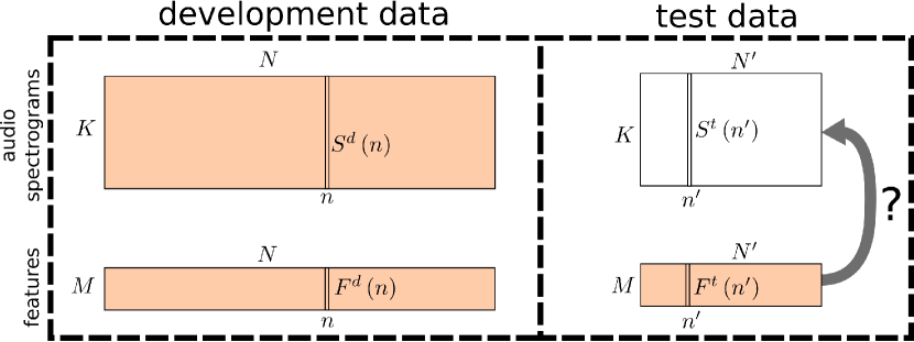
The proposed framework is summarized in Figure 1. We assume that an audio development database (dev-data) is available, which typically consists of several hours of continuous audio data.

In any case, this dev-data can be analyzed through a Short Term Fourier Transform (STFT), whose element-wise modulus is a $K\times N$ nonnegative matrix $S^{d}$, where $K$ and $N$ respectively denote the number of frequency bins and the number of frames. $S^{d}\left(n\right)$ and $F^{d}\left(n\right)$ will denote development data at frame $n$, understood as $K\times 1$ and $M\times 1$ vectors, respectively.

The main idea of this study is to consider that other observations of features $F^{t}$, of dimension $M\times N^{\prime}$ are available, which have been computed from an unknown underlying signal, whose $K\times N^{\prime}$ unknown magnitude spectrogram is denoted $S^{t}$. As highlighted in Figure 1, the main idea here is to use those test-features in conjunction with the dev-data so as to yield a meaningful estimate for $S^{t}$.

2 Estimation method

The proposed blind synthesis method operates on a frame-by-frame basis. For each given $M\times 1$ test frame $F^{t}\left(n^{\prime}\right)$ of features, it estimates the corresponding $K\times 1$ magnitude spectrum $S^{t}\left(n^{\prime}\right)$.

For one given test frame $n^{\prime}$, the chosen approach is to identify the $P$ feature frames among the dev-data, which are the most similar to $F^{t}\left(n^{\prime}\right)$, and to estimate $S^{t}\left(n^{\prime}\right)$ as the median of the $P$ corresponding development spectra. This technique is reminiscent from recent works in audio source separation [20, 21, 22], where magnitude spectrograms of background music are estimated as median values of properly chosen spectra.

Formally, let $\mathcal{X}$ bet a set of $M$ development audio segments $x_{m}$ for which both audio and the feature vectors $F(x_{m})$ are known. Let $s_{i}$ be a target segment for which only its feature vector $F(s_{i})$ is available, we are interested in finding:

$$\hat{s}_{i}=\arg\min_{x_{m}\in\mathcal{X}}\|F(s_{i})-F(x_{m})\|\text{\texttwosuperior}$$ (1)

let $d\left(f,f^{\prime}\right):\mathbb{R}^{M}\times\mathbb{R}^{M}\rightarrow\mathbb{R}^{+}$ be a known distance kernel, which indicates the difference between two feature vectors, both of dimension $M\times 1$. Many possible choices for such kernels are possible, such as the simple euclidean distance :

$$d\left(f,f^{\prime}\right)=\sqrt{\sum_{m=1}^{M}\left(f_{m}-f_{m}^{\prime}\right)^{2}}.$$

This choice of kernel assumes that all the features equally contribute to the metric which might not be the case. A weighted formulation of such distance between two feature vectors would thus be:

$$d_{W}(F(s),F(s^{\prime}))=\sqrt{\sum_{j=1}^{J}w_{j}\left(f_{j}(s)-f_{j}(s^{\prime})\right)^{2}}$$ (2)

where $W=[w_{j}]_{j=1..J}$ is a vector of weights to be determined. With these notations, finding the $P$ nearest neighbors of a segment $s$ amounts to finding the $P$ smallest elements in the set $D_{W}(s)=\{d_{W}\left(F(s),F(x_{m})\right)|x_{m}\in\mathcal{X}\}$.

Obviously, the features must be normalized. In the following, we will assume that all features have been standardized according to:

$$f_{j}(x_{k})\leftarrow\frac{f_{j}(x_{k})-\mu_{j}}{\sigma_{j}}$$

where $\mu_{k}$ and $\sigma_{j}$ are respectively the sample mean and standard deviation of the development data $\{f_{j}(x_{m})|x_{m}\in\mathcal{X}\}$. For each target segment $s$, we compute the $N\times 1$ vector $D_{s}$, whose $m^{\mbox{th}}$ entry is given by :

$$D_{s}\left(m\right)=d\left(F^{t}\left(s\right),F^{t}\left(x_{m}\right)\right),$$ (3)

and which basically gives the distance between current test feature vector and the entries of the development database. Then, the indexes of the $P$ smallest elements of $D_{s}$ are identified, yielding the indexes of the development frames which are most likely to be similar to current test frame.

Chapter 2 Synthesis methods

1 Concatenative Synthesis

1 Segment-by-segment approach

The simplest approach to synthesis is to work on each segment separately. An estimate of a signal $x$, sliced into $I$ segments $s_{i}$ whose positions $\{t_{i}\}_{i=1..I}$ are known, is obtained by replacing each segment $s_{i}$ by the smallest element $\hat{s}_{i}$ of $D(s_{i})$, relocated at $t_{i}$. This process yields an estimate $\hat{x}$ of $x$ defined by:

$$\hat{x}=[\hat{s}_{1}|\ldots|\hat{s}_{i}|\ldots|\hat{s}_{I}]$$ (1)

where:

$$\forall i\in[1..I],\hat{s}_{i}=\arg\min_{x_{m}\in\mathcal{X}}d_{W}\left(F(s_{i}),F(x_{m})\right)$$

This simple scheme is sufficient to perform some kind of cross-synthesis and we label this setup as the Cross-Plain method. Figure 1 shows an example of a target signal being synthesized using segments from the RWC Instrumental Piano dataset. In this setup, the nearest neighbor distance used relies only on the Chroma features (i.e. $w_{j}=1$ if $j\in[1..12]$, 0 otherwise).

Figure 1: Concatenative (cross) synthesis of a few seconds of blues from GTZAN base using segments from the RWC Instrumental (Piano) database. The mapping is performed using the Chroma vector computed through the Echo Nest API. Upper: original waveform, Middle: synthesis using the unaltered segments, Lower: synthesis using normalized and time-stretched segments.

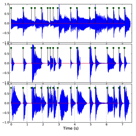
This simple example already raises some questions:

• How should the replacing segments $\hat{s}_{i}$ be normalized?

• Should the temporal alignment be somehow more relevant ? In particular, the replacing segments and the original ones may have very different length.

To address these issues, one may want to use the provided features to control the synthesis. For instance, the replacing segment may be transformed so that its resulting Loudness matches the target one (provided by the first Timbre coefficient). A precise morphing could additionally be controlled by the knowledge of the target Loudness peak location. Lower plot in Figure 1 shows an even simpler solution: segments are time-stretched to match their target’s length and normalization is achieved by ensuring all segments waveform have same peak value. We label this setup as the Cross-Normalized method

As one could expect, these simple processing tricks are not sufficient to reduce the main disturbing artifacts arising with such methods: brutal transitions between consecutive segments. Tackling this issue require either further processing of the transitions (e.g. fade-in/out) or modifying the segment selection criterion to enforce some kind of coherence between a chosen segment $\hat{s}_{i}$ and (at least) its neighbors $\hat{s}_{i-1}$ and $\hat{s}_{i+1}$.

2 Enforcing coherence, a regularization formulation

More generally, one can think of many ways to modify the selection according to various signal coherence criteria. The selection may then be expressed as a penalized version of (1):

$$\hat{s}_{i}=\arg\min_{x_{m}\in\mathcal{X}}d_{W}\left(F(s_{i}),F(x_{m})\right)+\lambda\mathcal{C}(x_{m},x)$$ (2)

where $\mathcal{C}$ can be any type of coherence cost between a sample $x_{m}$ and the target signal $x$ (e.g. a stretching cost, a loudness normalization cost, etc..). Expressing the concatenative synthesis problem as a set of constraints is the approach adopted for instance by Zils and Pachet in [23]. In their work, they also define sequence constraints to enforce some kind of continuity between the selected segments. In a similar manner, Schwarz [24] defines concatenative costs to assess the pertinence juxtaposing two segments.

A direct transposition of their methods to our setup is complex, since both method relies on the availability of more detailed features (e.g. pitch, spectral moments, etc..). Nonetheless, this pleads for longer-term considerations to be considered. Abundant literature can be found on the subject (interested reader may refer to the online survey maintained at IRCAM). An application to MSD-like features can be found in [15].

The nearest neighbor search yields for each target segment $s_{i}$ a set of $P$ candidates $\hat{s}_{i}^{p}$ with associated scores $v_{i}^{p}=d_{W}(F(s_{i}),F(\hat{s}_{i}^{p}))$. Instead of choosing the best candidate for each segment, one can search for an optimal sequence of candidates in the $P\times I$ grid. Given that a transition cost between two segment $\mathcal{C}(\hat{s}_{i},\hat{s}_{i+1})$ is defined, a Viterbi algorithm can be used to identify this optimal sequence. Possible choices for $\mathcal{C}(\hat{s}_{i},\hat{s}_{i+1})$ includes:

• The distance in the feature space $d_{W}\left(F(\hat{s}_{i}),F(\hat{s}_{i+1})\right)$

• A fixed penalty cost $\lambda_{v}$ whose value depend on a priori knowledge on segments similarities.

In this work, the audio datasets that we used are divided in audio files, corresponding to parts of (e.g. 30 seconds in GTZAN), whole songs (e.g. RWC Music Genre) or a chromatic scale played by a single instrument (RWC Instrumental Piano). To favor coherence of selected segments, we have investigated the following transition cost:

$$\mathcal{C}(\hat{s}_{i},\hat{s}_{i+1})=\begin{cases}0&\mbox{if }\hat{s}_{i}\mbox{ and}\hat{s}_{i+1}\mbox{ belong to the same file}\\ \lambda_{v}&\mbox{otherwise}\end{cases}$$

that favors the selection of segments belonging to the same audio file. We label the concatenative synthesis using a Viterbi algorithm and this transition cost as the Cross-Penalized method.

2 Additive Synthesis

We have investigated a different approach, labeled additive synthesis. Contrary to the concatenative synthesis where a single candidate per segment is retained, additive synthesis will use a collection of examples for each segment in order to build an estimate. Combining those elements though, is not a trivial issue. A simple summation in the time domain will give unsatisfactory results. The re-synthesized signal can be modeled as a mixture of $P$ samples. Such mixture is better expressed in the time-frequency domain. This technique is inspired by recent works in audio source separation [22, 21].

Let $s_{i}$ be a segment and $S_{i}$ be the modulus of its Short Term Fourier Transform (STFT). The set of the $P$ smallest elements in $D_{W}(s_{i})$ defines a set of $P$ segments $\{s_{i}^{p}\}_{p=1..P}$ with STFT modulus $\{S_{i}^{p}\}_{p=1..P}$. Since all these elements are nonnegative, any positive combination of them remains nonnegative and can therefore be considered as an estimated STFT modulus $\hat{S}_{i}$. In this work, three types of combinations have been considered:

$$\hat{S}_{i}^{median} =\mbox{median}_{p=1..P}\{S_{i}^{p}\}$$ (3)

$$\hat{S}_{i}^{mean} =\frac{1}{P}\sum S_{i}^{p}$$ (4)

$$\hat{S}_{i}^{max} =\max_{p=1..P}\{S_{i}^{p}\}$$ (5)

$\hat{S}_{i}^{median}$ was the only one being considered, for it’s ability to discard outliers. However, experiments showed that in some situations, the opposite strategy of favoring outliers (i.e. $\hat{S}_{i}^{max}$) gives interesting results. Finally, using $\hat{S}_{i}^{mean}$ realizes a compromise between the two former strategies. Once a STFT modulus $\hat{S}_{i}$ has been estimated, direct inversion is not possible since the phase information is missing. In order to build a corresponding audio waveform, some iterations of the classical Griffin and Lim algorithm[25] can be used. We label the synthesis using (7), (8) and (9) respectively, followed by a Griffin and Lim reconstruction as Add-Median, Add-Mean and Add-Max methods.

Chapter 3 Evaluation

1 Speech synthesis from standard audio features

1 Experimental setup

In this section, we propose an evaluation of the proposed method in the context of speech synthesis. For this purpose, the dev-data considered is a concatenation of $10$s excerpts taken randomly from the Voxforge corpus., which consists of more than $3$ hours of speech signals uttered both by male and female speakers and sampled at $36$kHz. A STFT is computed on the resulting waveform, with frames of $32$ms (leading to $K=256$) and a hopsize of $4$ms. $N$ depends on the size of the development data and is one of the parameters of this evaluation.

The test data is chosen as another excerpt from the Voxforge corpus, and corresponds to a sentence not found in the dev-data, being uttered by a speaker also excluded from the dev-data.

The same features were computed on both the development and test data using the YAAFE toolbox [2]. Depending on $M$, common features were computed, as explained in Table 1. As can be seen, the $8$ first features were purposefully chosen as highly non-invertible and the MFCC were chosen if $M$ gets higher, due to their widespread use in speech processing.

In this experiment, we perform synthesis using the Add-median method described in previous section.

$M=3$	Zero crossing rate Onset detection function Energy by frame
$M=8$	Those above plus spectral slope, centroid, spread and flux
$M=11$	Those above plus the $3$ first Mel-Frequency Cepstral Coefficients (MFCC)
$M=21$	Those above plus $10$ more MFCC

Table 1: Features computed depending on $M$.

We report performance of the proposed method for varying sizes $N$ of the development database, a varying number $M$ of features and a varying number $P$ of neighbors selected for estimation. As an objective metric, we consider the relative error $20\log_{10}\frac{\left\|S^{t}-\hat{S^{t}}\right\|_{F}}{\left\|S^{t}\right\|_{F}}$ between original and estimated test spectrograms, where $\left\|\cdot\right\|_{F}$ denotes the Frobenius norm (root sum of squares). For each choice of $\left(M,N,P\right)$, $100$ independent tests were performed and $E\left(M,N,P\right)$ is defined as the corresponding average of the error obtained on all these tests.

Even if this objective metric somewhat captures quality of reconstruction, it is understood that only listening tests are fully relevant to evaluate performance. To this purpose, a complete MATLAB implementation of the proposed method, release under a BSD license, along with examples of reconstructed signals are available on the webpage dedicated to this paper.

To the best of our knowledge, no other blind features inversion technique similar to the one presented here has been presented so far and we hence cannot compare its performance to previous comparable work. Still, we chose to compare it nonetheless with an MFCC inversion technique [11] on the same data, which generates an audio signal based on a sequence of MFCC, using explicit knowledge of the way they are computed, as opposed to the blind inversion method described here.

2 Results

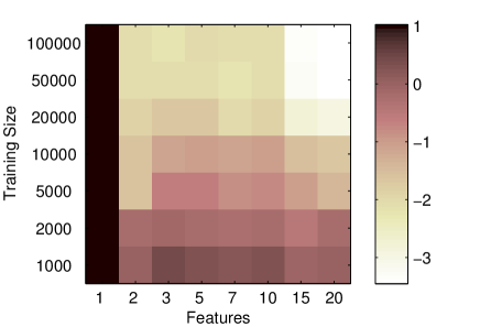
In figure 1 (top), relative reconstruction error $E\left(M,N,P\right)$ is displayed as a function of $M$ and $N$, with $P=10$ being fixed. As can be seen, increasing both $M$ and $N$ yields better results. Very interestingly, it can be seen that the proposed method provides performance which is comparable to the deterministic inversion of the MFCC, provided $M$ and $N$ are sufficiently large. This result is very encouraging, since it means that blind inversion is indeed a viable alternative to informed inversion approaches which are dedicated to some specific features only.

In figure 1 (bottom) is displayed $E\left(M,N,P\right)$ as a function of $P$ alone, with $M=8$ and $N=10^{5}$ being fixed. As can be seen, the number of selected neighbors needs to be high enough so as to smooth spurious matches, but also needs to be small enough so as not to end up with an almost constant resulting estimated spectrogram. However, performance of the method was found to be rather robust to the choice of this parameter, and $P=10$ generally seems like a good compromise.

Figure 1: Objective results: performance of the proposed method as a function of the number of development frames $N$ and number of features $M$, with $P=10$ fixed.

Figure 2: Influence of $P$ on the reconstruction quality with $M=7$ and $N=10^{5}$ being fixed.

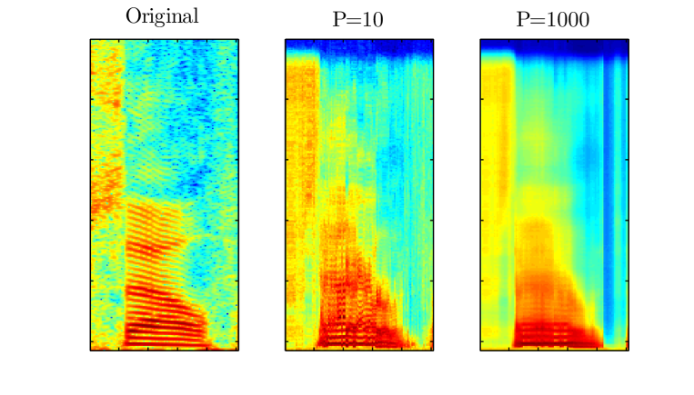
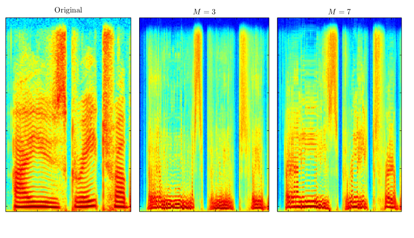
In figure 3 is displayed one particular example of reconstructed spectrogram using $N=10^{5}$ development frames, $P=10$ and a varying number of features. As can be seen, the estimated spectrogram is very similar to the original one, using only highly non-invertible features.

Figure 3: Typical reconstruction of a spectrogram using the proposed approach with a development databased composed of $N=10^{5}$ frames, corresponding to $6.6$min of continuous audio. Up : original (unknown) test spectrogram to be estimated. Middle : estimate using $M=3$ features (zero-crossing rate, onset detection function and frame energy). Down : reconstruction using $M=8$ features ($M=3+$spectral centroid, slope, flux and spread).

2 Inverting MSD songs

1 Overview of MSD features

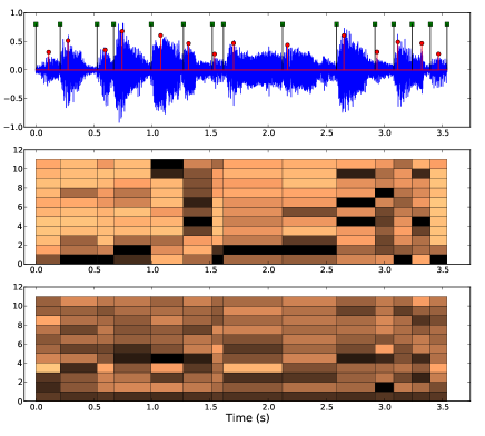
As explained on the MSD website, a signal $x$ is first sliced into $I$ non overlapping segments:

$$x = [s_{1}|\ldots|s_{i}|\ldots|s_{I}]$$ (1)

For each segment 27 acoustic features are computed (see [15, 26, 13] for more details):

• 12 chroma coefficients $\{f_{j}\}_{j=1:12}$ describing the harmonic content of the segment.

• 12 timbre coefficients $\{f_{j}\}_{j=13:24}$ describing the sound texture by quantifying its spectro-temporal shape.

• 3 Loudness coefficients : value at start $f_{25}$, value at peak $f_{26}$ and peak position $f_{27}$. Loudness corresponds to the perceived energy of the signal and relies on a bark scale nonlinear mapping of the signal spectrum.

The feature vector $F(s)$ for a segment $s$ thus have the following structure:

$$F(s) =[f_{1}(s)|\ldots|f_{j}(s)|\ldots|f_{J}(s)]$$ (2)

where $f_{j}(s)$ is the $j$-th feature of the segment $s$ and $J=27$. In addition, the segmentation is provided in the form of the set $\{t_{i}\}_{i=1..I}$ of segment start instants. In average, there are about 4 segments per second, but this may vary a lot depending on signal nature (e.g. music tempo and rhythm). Figure 4 presents an overview of these features for a short audio excerpt. In the given example, the total number of acoustic features available is around 100 for one second of signal sampled at 44100 Hz. This drastic dimensionality reduction is obviously a lossy process.

Figure 4: Visualization of features fetched from the Echo Nest online API for a short excerpt taken from the RWC database. Upper plot shows the waveform. Segments boundaries are figured with green squares, loudness peaks with red circles. The middle plot corresponds to the Chroma features ($f_{1}$ to $f_{12}$) and the lower one to Timbre coefficients ($f_{13}$ to $f_{24}$)

2 Experimental setup

As explained in [17] (see also Chapter 6 in [15]), results obtained through concatenative synthesis methods can generally be considered a different piece of music. Therefore, measuring the adequacy of the synthesized audio to the target is a challenging issue that may require the use of a sound taxonomy, or carefully designed listening tests.

Objective evaluation may yet be possible, when the original audio is available, e.g. by using a distance in the time-frequency domain between the original $S$ and an estimated STFT modulus $\hat{S}$. A first idea would be to measure a mean-square error:

$$MSE(S,\hat{S})=10\log_{10}\frac{\|S-\hat{S}\|_{F}}{\|S\|_{F}}$$ (3)

where $\|.\|_{F}$ stands for the Frobenius norm or the sum of the squares. For audio spectrograms, it is more relevant to measure the Kullback-Leibler (KL) divergence of the normalized magnitude spectrograms, seen as probability density functions:

$$KL(S_{N},\hat{S}_{N})=\sum_{n=1}^{L}\sum_{k=1}^{K}S_{N}(k,n)\log\left(\frac{S_{N}(k,n)}{\hat{S}_{N}(k,n)}\right)$$ (4)

where $n$ and $k$ are respectively the discrete time and frequency index of the spectrograms, and normalization is achieved by:

$$S_{N}(k,n)=\frac{S(k,n)}{\sum_{n}\sum_{k}S(k,n)}$$ (5)

We have used the provided API to gather features for the RWC Music Genre (RWC-MDB-G-2001-M01$\sim$M09, 100 files), Instrumental Piano (RWC-MDB-I-2001 n1$\sim$12, 12 files) and GTZAN (1000 files) datasets. Combined, we have a collection $\mathcal{X}$ of $M_{max}\simeq 170000$ segments corresponding to approximately 20 hours of audio data. Since we need the real audio data for objective performance measurements, we use part of this database for the test. Nonetheless, any of the synthesis method can straightforwardly be applied to a file in the MSD format (see the companion website for examples).

A development set $\mathcal{X}_{dev}\subset\mathcal{X}$ of $M$ segments is first drawn by selecting files at random in the complete collection. And the synthesis is evaluated on a 20-segment length excerpt $x_{test}$ chosen in a random file from the complementary set $\mathcal{X}_{test}=\overline{\mathcal{X}}_{dev}$. To ensure that no exactly similar segments are simultaneously present in the train and test sets (due to some redundancies in the GTZAN dataset), we remove all segments belonging to the same genre as $x_{test}$. We investigate the following parameters:

• Synthesis method: 6 of them are considered: 3 concatenative ones (Cross-Plain, Cross-Normalized and Cross-Penalized, 3 additive ones (Add-Mean, Add-Max and Add-Median) and a parametric one for comparison obtained using the software provided by D. Ellis.

• Combination of features used in the nearest neighbor search.

• Number of neighbors considered $P$.

3 Results

Audio examples

The concatenative synthesis methods Cross-Plain, Cross-Normalized and Cross-Penalized perform erratically relative to the spectrogram reconstruction metric (4). We provide as many sound examples as possible (both from our own dataset and the MSD) of the synthesis results on a companion website. Depending on the chosen method, very different types of results can be obtained. This diversity of synthesis is better appreciated by listening to examples. Nonetheless, some interesting observations can be made with objective measurement of additive synthesis experiments.

Influence of the feature combination

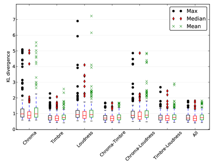
The size of the development set is fixed to $M=100000$. We investigate the 7 possible combinations of the three types of features (Chroma, Timbre, Loudness). For each feature combination, 100 tests are run, 25 for each value of $P$ among $\{1,5,10,20\}$.

Figure 5 shows the normalized spectrogram KL divergence between original and resynthesized results for the different combinations of features and STFT modulus combining strategies. Timbre coefficients seem more robust to the task than Chroma and Loudness ones. Best results are arguably reached using Timbre+Chroma features, and using Loudness features does not seem to improve the results in any case. This experiments also shows that there seem not to be a significant difference between the STFT modulus combining strategies, although the synthesis may sound quite different.

Figure 5: KL divergence between normalized spectrogram of original and reconstruction with (7), (8) and (9), results for 100 tests for each of the 7 features combinations. Timbre features seem to be the most effective ones.

Influence of $P$

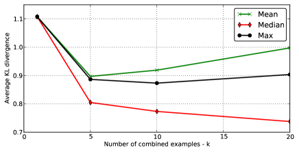
With the same experimental setup, we can observe results marginalized over $P$. Figure 6 summarizes the observations. The fact that Mean and Max strategies seem to perform slightly worse when $P>5$ is mainly due to the presence of outliers. This corresponds to situations where one or more of the candidate is poorly correlated but still takes over the other ones, this scenario being unlikely to appear in the case of the median.

Figure 6: KL divergence of reconstructed STFT modulus for various number of considered examples.

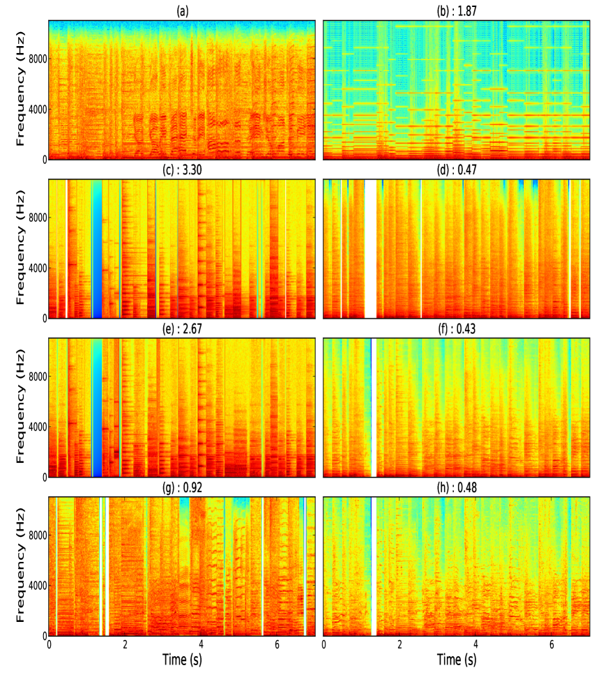
Finally, Figure 7 present the spectrograms for an example for the 6 proposed strategies and the baseline parametric synthesis. The corresponding sounds as well as many more examples are available on the companion website.

Figure 7: Logarithm of the STFT modulus of (a) original, (b) parametric synthesis using D. Ellis Matlab code. (c) Cross-Plain and (e) Cross-Normalized (using only RWC Instrumental Piano for $\mathcal{X}_{dev}$), (g) Cross-Penalized (using all dataset), (d) Add-Median, (f) Add-Mean and (h) Add-Max for $P=10$. All nearest neighbor search used the Chroma-Timbre combination except (c) and (e) for which only the Chroma were used. Displayed values are the corresponding KL divergence scores (4).

Conclusion

In this work, we present some early attempts to resynthesize audio from scarce, non-uniformly distributed, arbitrary features as one can found in the MSD. Synthesis is achieved through the use of a development dataset for which the audio is available. After applying state of the art approaches of concatenative synthesis to this context, we propose a different scheme of additive synthesis that seems to help achieve a pertinent reconstruction of the magnitude spectrogram.

Many improvements can be thought of. First of all, more data may be needed. Raising the development dataset from 20 to 200 or even 2000 hours of audio would certainly improve the quality of the reconstruction. Second, our methods are based on a purely non-supervised neighbor search algorithm, obviously one could try supervised or semi-supervised methods. Additionally, the weights of the distance kernel in 2 could be learned to improve the pertinence of the selection.

Future work will investigate these points. As one may notice, no use is made in this work of all the metadata available in the MSD, nor of other types of features such as tempo, beats etc.. Arguably the reconstruction could benefit from this additional information. Finally, other types of signal coherence constraints might be expressed as regularizations of problem (2) (e.g. sparsity -or structured sparsity - of the reconstructed spectrogram in a given dictionary). MSD resynthesis remains a highly challenging issue, but not an impossible one.

References

- [1] M. McKinney and J. Breebaart, “Features for audio and music classification,” in Proceedings of the International Society for Music Information Retrieval Conference (ISMIR), vol. 3, pp. 151–158, 2003.
- [2] B. Mathieu, S. Essid, T. Fillon, J. Prado, and G. Richard, “Yaafe, an easy to use and efficient audio feature extraction software,” in Proceedings of the 11th International Society for Music Information Retrieval Conference (ISMIR), 2010.
- [3] C. Wang and L. Avery, “An industrial strength audio search algorithm,” in Proceedings of the International Society for Music Information Retrieval Conference (ISMIR), vol. 3, 2003.
- [4] R. Miotto and N. Orio, “A music identification system based on chroma indexing and statistical modeling,” in Proceedings of the International Conference on Music Information Retrieval, pp. 301–306, 2008.
- [5] E. Dupraz and G. Richard, “Robust frequency-based audio fingerprinting,” in IEEE International Conference on Acoustics, Speech and Signal Processing (ICASSP), pp. 281–284, IEEE, 2010.
- [6] S. Fenet, G. Richard, and Y. Grenier, “A scalable audio fingerprint method with robustness to pitch-shifting,” in Proceedings of the 12th International Conference on Music Information Retrieval (ISMIR), 2011.
- [7] L. Rabiner and B. Juang, “Fundamentals of speech recognition,” 1993.
- [8] D. Chazan, R. Hoory, G. Cohen, and M. Zibulski, “Speech reconstruction from mel frequency cepstral coefficients and pitch frequency,” in IEEE International Conference on Acoustics, Speech and Signal Processing (ICASSP), vol. 3, pp. 1299–1302, IEEE, 2000.
- [9] B. Milner and X. Shao, “Speech reconstruction from mel-frequency cepstral coefficients using a source-filter model,” in International Conference on Spoken Language Processing (ICSLP), pp. 2421–2424, Citeseer, 2002.
- [10] X. Shao and B. Milner, “Pitch prediction from mfcc vectors for speech reconstruction,” in IEEE International Conference on Acoustics, Speech and Signal Processing (ICASSP), vol. 1, pp. I–97, IEEE, 2004.
- [11] D. Ellis, “PLP and RASTA (and MFCC, and inversion) in Matlab,” 2005. online web resource.
- [12] B. Milner and X. Shao, “Clean speech reconstruction from mfcc vectors and fundamental frequency using an integrated front-end,” Speech Communication, vol. 48, no. 6, pp. 697–715, 2006.
- [13] T. Bertin-Mahieux, D. Ellis, B. Whitman, and P. Lamere, “The million song dataset,” in International Society for Music Information Retrieval Conference, 2011.
- [14] “The Echo Nest Analize, API,” in http://developer.echonest.com.
- [15] T. Jehan, Creating music by listening. PhD thesis, Massachussets Institute of Technology, 2005.
- [16] D. Ellis, “PLP and RASTA (and MFCC, and Inversion) in Matlab,” in http://www.ee.columbia.edu/~dpwe/resources/matlab/rastamat/, 2005.
- [17] D. Schwarz, “Concatenative sound synthesis: The early years,” Journal of New Music Research, vol. 35, pp. 3–22, Mar. 2006.
- [18] M. Goto and H. Hashiguchi, “RWC music database: Music genre database and musical instrument sound database,” in Proc. ISMIR, no. October, pp. 229–230, 2003.
- [19] G. Tzanetakis and F. Cook, “Sound analysis using MPEG compressed audio,” in IEEE International Conference on Acoustics, Speech and Signal Processing, vol. 2, pp. 761–764, 2000.
- [20] Z. Rafii and B. Pardo, “Music/voice separation using the similarity matrix,” in Proceedings of the 13th International Conference on Music Information Retrieval (ISMIR), pp. 583–588, 2012.
- [21] A. Liutkus, Z. Rafii, R. Badeau, B. Pardo, and G. Richard, “Adaptive filtering for music/voice separation exploiting the repeating musical structure,” in IEEE International Conference on Acoustics, Speech and Signal Processing, pp. 53–56, 2012.
- [22] D. Fitzgerald, “Vocal Separation Using Nearest Neighbours and Median Filtering,” in Irish Signal and Systems Conference, pp. 583–588, 2012.
- [23] A. Zils and F. Pachet, “Musical mosaicing,” in Digital Audio Effects (DAFx), pp. 1–6, 2001.
- [24] D. Schwarz, “A system for data-driven concatenative sound synthesis,” Digital Audio Effects (DAFx), pp. 1–6, 2000.
- [25] D. Griffin and J. Lim, “Signal estimation from modified short-time Fourier transform,” IEEE Transactions on Acoustics, Speech and Signal Processing, vol. 32, no. 2, pp. 236–243, 1984.
- [26] D. Ellis, B. Whitman, T. Jehan, and P. Lamere, “The echo nest musical fingerprint,” in International Society for Music Information Retrieval Conference, vol. 32, 2010.