Graph Laplacians and discrete reproducing kernel Hilbert spaces from restrictions

Abstract.

We study kernel functions, and associated reproducing kernel Hilbert spaces $\mathscr{H}$ over infinite, discrete and countable sets $V$. Numerical analysis builds discrete models (e.g., finite element) for the purpose of finding approximate solutions to boundary value problems; using multiresolution-subdivision schemes in continuous domains. In this paper, we turn the tables: our object of study is realistic infinite discrete models in their own right; and we then use an analysis of suitable continuous counterpart problems, but now serving as a tool for obtaining solutions in the discrete world.

1. Introduction

In a number of recent papers, kernel tools have found new applications, and a number of them depend on an interplay between continuous vs discrete; so between, (i) more classical continuous kernel models, and (ii) various discretization procedures; see the citations below. Applications of kernel tools include optimization, maximum-likelihood constructs, and machine learning models; they all entail a combination of analysis tools for a variety of reproducing kernels, and the associated reproducing kernel Hilbert spaces (RKHS); as well as probabilistic sampling and estimation; – all issues involving theorems for RKHSs. So far the emphasis has been on the continuous models, and we shall turn the table in the present paper. We shall make use of a class of discrete RKHSs which are typically associated with Gaussian free fields, and determinantal point process, and associated determinantal measures. The purpose of our paper is to offer a systematic approach to these questions. Our approach is motivated in part by the way the classical Cameron-Martin RKHS is used in the analysis of Brownian motion, and related Gaussian processes. We are concerned with a characterization of those RKHSs $\mathscr{H}$ of functions, on some state space $V$, which contain the Dirac masses $\delta_{x}$ for all points $x$ in $V$.

Our setting is that of infinite discrete models vs their continuous counterparts. Our discrete analysis setting is as follows: Given is an infinite set $V$ of vertices, and a set $E$ of edges, contained in $V\times V\backslash\left\{\mbox{the diagonal}\right\}$. Further, a positive symmetric function $c$ on $E$ is prescribed ($c$ is conductance in electrical networks), and there is a resulting graph Laplacian. Its spectral theory will be considered. In this setting, we arrive at a host of network models, whose analysis all involve kernels. Connectedness for our infinite graphs will be assumed. The relevant RKHSs are certain discrete Dirichlet spaces $\mathscr{H}_{\left(E,c\right)}$ consisting of finite energy-functions, and modeled on the classical Cameron-Martin spaces; these discrete variants are Hilbert spaces of functions on $V$ (modulo constants), and depending on the choice of $\left(V,E,c\right)$. It is always the case that the differences $f\left(x\right)-f\left(y\right)$ for $f$ in $\mathscr{H}_{\left(E,c\right)}$, for any given pair of vertices $x$ and $y$, is well behaved: The differences (voltage-drop) will be represented by a kernel (in $\mathscr{H}_{\left(E,c\right)}$), depending on the pair $x$, $y$. By contrast, point-evaluation itself (for a single vertex) does not automatically have a kernel representation by a function in $\mathscr{H}_{\left(E,c\right)}$.

Our first result (2.9) gives a necessary and sufficient condition for existence of $\mathscr{H}_{\left(E,c\right)}$-kernels for point-evaluation, so a kernel associated to a fixed vertex $x_{0}$. It follows from this that, when a vertex $x_{0}$ is given, the answer to this question involves the entire vertex-set $V$, so including distant vertices and also boundary considerations. The question of deciding existence of finite-energy point-kernels has applications. For example, each setting sketched above gives rise to an associated Markov chain model involving a reversible random walk. It is known that the random walk is transient if and only if finite-energy point-kernels exist.

In Sections 4-6, we turn to a family of generalized Cameron-Martin spaces; – in Theorems 4.13 and 6.8, we give an explicit comparison between the continuous vs the discrete variants.

A reproducing kernel Hilbert space (RKHS) is a Hilbert space $\mathscr{H}$ of functions on a prescribed set, say $V$, with the property that point-evaluation for $f\in\mathscr{H}$ is continuous with respect to the $\mathscr{H}$-norm. They are called kernel spaces, because, for every $x\in V$, the point-evaluation for functions $f\in\mathscr{H}$, $f\left(x\right)$ must then be given as a $\mathscr{H}$-inner product of $f$ and a vector $k_{x}$, in $\mathscr{H}$; called the kernel. See (2.4) below.

Background. RKHSs have been studied extensively since the pioneering papers by Aronszajn in the 1940ties, see e.g., [Aro43, Aro48]. They further play an important role in the theory of partial differential operators (PDO); for example as Green’s functions of second order elliptic PDOs; see e.g., [Nel57, HKL⁺14, Trè06]. Other applications include engineering, physics, machine-learning theory (see [KH11, SZ09, CS02]), stochastic processes (e.g., Gaussian free fields), numerical analysis, and more. See, e.g., [AD93, ABDdS93, AD92, AJSV13, AJV14, BTA04]. Also, see [LB04, HQKL10, ZXZ12, LP11, Vul13, SS13, HN14]. But the literature so far has focused on the theory of kernel functions defined on continuous domains, either domains in Euclidean space, or complex domains in one or more variables. For these cases, the Dirac $\delta_{x}$ distributions do not have finite $\mathscr{H}$-norm. But for RKHSs over discrete point distributions, it is reasonable to expect that the Dirac $\delta_{x}$ functions will in fact have finite $\mathscr{H}$-norm.

Here we consider the discrete case, i.e., RKHSs of functions defined on a prescribed countable infinite discrete set $V$. We are concerned with a characterization of those RKHSs $\mathscr{H}$ which contain the Dirac masses $\delta_{x}$ for all points $x\in V$. Of the examples and applications where this question plays an important role, we emphasize two: (i) discrete Brownian motion-Hilbert spaces, i.e., discrete versions of the Cameron-Martin Hilbert space [Fer03, HH93]; (ii) energy-Hilbert spaces corresponding to graph-Laplacians.

Our setting is a given positive definite function $k$ on $V\times V$, where $V$ is discrete (see above). We study the corresponding RKHS $\mathscr{H}\left(=\mathscr{H}\left(k\right)\right)$ in detail.

A positive definite kernel $k$ is said to be universal [CMPY08] if, every continuous function, on a compact subset of the input space, can be uniformly approximated by sections of the kernel, i.e., by continuous functions in the RKHS. We show that for the RKHSs from kernels $k_{c}$ in electrical network $G$ of resistors, this universality holds. The metric in this case is the resistance metric on the vertices of $G$, determined by the assignment of a conductance function $c$ on the edges in $G$, see 6 below.

The problems addressed here are motivated in part by applications to analysis on infinite weighted graphs, to stochastic processes, and to numerical analysis (discrete approximations), and to applications of RKHSs to machine learning. Readers are referred to the following papers, and the references cited there, for details regarding this: [AJS14, AJ12, AJL11, JPT15, JP14, JP11a, DG13, Kre13, ZXZ09, Nas84, NS13].

Infinite Networks. While the natural questions for the case of large (or infinite) networks, “the discrete world,” have counterparts in the more classical context of partial differential operators/equations (PDEs), the analysis on the discrete side is often done without reference to a continuous PDE-counterpart.

The purpose of the present paper is to try to remedy this, to the extent it is possible. We begin with the discrete context (2.9). And we proceed to show that, in the discrete case, our analysis depends on two tools, (i) positive definite (p.d.) functions, and associated RKHSs, and (ii) (resistance) metrics. Both may be studied as purely discrete objects, but nonetheless, in several of our results (including the corollaries in Sections 5 and 6), we give contexts for continuous counterparts to the two discrete tools, (i) and (ii). We make precise how to use the continuous counterparts for computations in explicit discrete models, and in the associated RKHSs.

In Theorems 4.13 and 6.4 we give such concrete (countable infinite) discrete models which can be understood as restrictions of analogous PDE-models. In traditional numerical analysis, one builds clever discrete models (finite element methods) for the purpose of finding approximate solutions to PDE-boundary value problems. They typically use multiresolution-subdivision schemes, applied to the continuous domain, subdividing into simpler discretized parts, called finite elements. And with variational methods, one then minimize various error-functions. In this paper, we turn the tables: our object of study are the discrete models, and analysis of suitable continuous PDE boundary problems serve as a tool for solutions in the discrete world.

2. Discreteness in reproducing kernel Hilbert spaces

Definition 2.1.

Let $V$ be a set, and $\mathscr{F}\left(V\right)$ denotes the set of all finite subsets of $V$. A function $k:V\times V\rightarrow\mathbb{C}$ is said to be positive definite, if

$$\underset{\left(x,y\right)\in F\times F}{\sum\sum}k\left(x,y\right)\overline{c_{x}}c_{y}\geq 0$$ (2.1)

holds for all coefficients $\{c_{x}\}_{x\in F}\subset\mathbb{C}$, and all $F\in\mathscr{F}\left(V\right)$.

Definition 2.2.

Fix a countable infinite set $V$.

1. For all $x\in V$, set

   $$k_{x}:=k\left(\cdot,x\right):V\rightarrow\mathbb{C}$$ (2.2)

   as a function on $V$.

2. Let $\mathscr{H}:=\mathscr{H}\left(k\right)$ be the Hilbert-completion of the $span\left\{k_{x}:x\in V\right\}$, with respect to the inner product

   $$\left\langle\sum_{x\in F}c_{x}k_{x},\sum_{y\in F}d_{y}k_{y}\right\rangle_{\mathscr{H}}:=\underset{F\times F}{\sum\sum}\overline{c_{x}}d_{y}k\left(x,y\right),\quad F\in\mathscr{F}\left(V\right),$$ (2.3)

   modulo the subspace of functions of zero $\mathscr{H}$-norm, i.e.,

   $$\underset{F\times F}{\sum\sum}\overline{c_{x}}c_{y}k\left(x,y\right)=0.$$

   $\mathscr{H}$ is then a reproducing kernel Hilbert space (RKHS), with the reproducing property:

   $$\left\langle k_{x},\varphi\right\rangle_{\mathscr{H}}=\varphi\left(x\right),\quad\forall x\in V,\>\forall\varphi\in\mathscr{H}.$$ (2.4)

3. If $F\in\mathscr{F}\left(V\right)$, set $\mathscr{H}_{F}=\text{closed\>\ span}\{k_{x}\}_{x\in F}\subset\mathscr{H}$, (closed is automatic as $F$ is finite.) And set

   $$P_{F}:=\text{the orthogonal projection onto $\mathscr{H}_{F}$}.$$ (2.5)

Remark 2.3.

The summations in (2.3) are all finite. We use physicists’ convention, so that the inner product in (2.3) is conjugate linear in the first variable, and linear in the second variable.

We shall need the following lemma:

Lemma 2.4.

Let $k:V\times V\rightarrow\mathbb{C}$ be a positive definite kernel, and let $\mathscr{H}$ be the corresponding RKHS. Then a function $\xi$ on $V$ is in $\mathscr{H}$ if and only if there is a constant $C<\infty$ such that, for all finite subsets $F\subset V$, and all $\left\{c_{x}\right\}_{x\in F}\subset\mathbb{C}^{\#F}$, we have:

$$\left|\sum_{x\in F}c_{x}\xi\left(x\right)\right|^{2}\leq C\underset{F\times F}{\sum\sum}\overline{c_{x}}c_{y}k\left(x,y\right).$$ (2.6)

Proof.

See [Aro48]. ∎

A reproducing kernel Hilbert space (RKHS) is a Hilbert space of functions on some set $S$. If $S$ comes with a topology, it is natural to study RHHSs $\mathscr{H}$ consisting of continuous functions on $S$. If $k$ is continuous on $S\times S$, one can show that then the functions in $\mathscr{H}\left(k\right)$ are also continuous. Except for trivial cases, the Dirac “function”

$$\delta_{x}\left(y\right)=\begin{cases}1&y=x\\ 0&y\neq x\end{cases}$$ (2.7)

is not continuous, and as a result, $\delta_{x}$ will typically not be in $\mathscr{H}$. But the situation is different for discrete spaces.

We will show that, even if $S$ is a given discrete set (countable infinite), we still often have $\delta_{x}\notin\mathscr{H}$ for naturally arising RKHSs $\mathscr{H}$; see also [JT15].

Below, we shall concentrate on cases when $S=V$ is a set of vertices in a graph $G$ with edge-set $E\subset V\times V\backslash\left(\text{diagonal}\right)$, and on classes of RKHSs $\mathscr{H}$ of functions on $V$, for which $\delta_{x}\in\mathscr{H}$ for all $x\in V$.

Definition 2.5.

The RKHS $\mathscr{H}$ (in Def. 2.2) is said to have the discrete mass property if $\delta_{x}\in\mathscr{H}$, for all $x\in V$. $\mathscr{H}$ is then called a discrete RKHS.

The following is immediate.

Proposition 2.6.

Suppose $\mathscr{H}$ is a discrete RKHS of functions on a vertex-set $V$, as described above; then there is a unique operator $\Delta$, with dense domain $dom\left(\Delta\right)\subset\mathscr{H}$, such that

$$\left(\Delta f\right)\left(x\right)=\left\langle\delta_{x},f\right\rangle_{\mathscr{H}},\quad\text{for all $x\in V$, and all $f\in dom\left(\Delta\right)$.}$$ (2.8)

The operator $\Delta$ from (2.8) will be studied in detail in 5 below. In special cases, it is called a graph-Laplacian; and it is a discrete analogue of the classical Laplace operator $-\nabla^{2}$.

Corollary 2.7.

Let $k:V\times V\rightarrow\mathbb{C}$, $\#V=\aleph_{0}$, be a positive definite function, and let $\mathscr{H}$ be the corresponding RKHS. Assume $\delta_{x}\in\mathscr{H}$ for all $x\in V$; then there are closable operators

$$\mathscr{H}\xrightarrow{\;T\;}l^{2}\left(V\right),\quad\mbox{and}\quad l^{2}\left(V\right)\xrightarrow{\;S\;}\mathscr{H},$$ (2.9)

such that $T\subseteq S^{*}$, $S\subseteq T^{*}$; and

$$T\,k_{x}=\delta_{x},\;S\,\delta_{x}=\delta_{x},\;\mbox{for all $x\in V$.}$$ (2.10)

Proof.

By assumption, $S$ and $T$ are well defined as specified in (2.9)-(2.10), with

$$dom\left(T\right) =span\left\{k_{x}\>:\>x\in V\right\} \mathscr{H}$$ dense in ; and

$$dom\left(S\right) =span\left\{\delta_{x}\>:\>x\in V\right\} l^{2}\left(V\right)$$ dense in .

By 2.6, we have

$$\left\langle Tf,\varphi\right\rangle_{l^{2}}=\left\langle f,S\varphi\right\rangle_{\mathscr{H}},$$ (2.11)

for all $f\in dom\left(T\right)\subset\mathscr{H}$, and all $\varphi\in dom\left(S\right)\subset l^{2}$.

The conclusions $T\subset S^{*}$, and $S\subset T^{*}$, follow from (2.11). Since each operator $S$ and $T$ has dense domain, it follows that both $T^{*}$ and $S^{*}$ must have dense domains in the respective Hilbert spaces, i.e., $dom\left(T^{*}\right)$ dense in $l^{2}$, and $dom\left(S^{*}\right)$ dense in $\mathscr{H}$. ∎

Remark 2.8.

As a result, we conclude that $T^{*}\overline{T}$ is a selfadjoint extension of the operator $\Delta$ from 2.6.

Theorem 2.9.

Given $V$, and a positive definite (p.d.) function $k:V\times V\rightarrow\mathbb{R}$, let $\mathscr{H}\left(=\mathscr{H}\left(k\right)\right)$ be the corresponding RKHS. Fix $x_{1}\in V$; then the following three conditions are equivalent:

1. $\delta_{x_{1}}\in\mathscr{H}$;

2. $\exists\,0\leq C_{x_{1}}<\infty$, such that

   $$\left|\xi\left(x_{1}\right)\right|^{2}\leq C_{x_{1}}\underset{F\times F}{\sum\sum}\overline{\xi\left(x\right)}\xi\left(y\right)k\left(x,y\right)$$ (2.12)

   holds, for all $F\in\mathscr{F}\left(V\right)$, and all functions $\xi$ on $F$.

3. For $F\in\mathscr{F}\left(V\right)$, set

   $$K_{F}:=\left(k\left(x,y\right)\right)_{\left(x,y\right)\in F\times F},$$ (2.13)

   as a $\#F\times\#F$ matrix. Then

   $$\sup_{F\in\mathscr{F}\left(V\right)}\left(K_{F}^{-1}\delta_{x_{1}}\right)\left(x_{1}\right)<\infty.$$ (2.14)

Proof.

(1)$\Longrightarrow$(2) We use 2.4. Let $\xi$ be any function on $F\in\mathscr{F}\left(V\right)$, and set

$$h_{\xi}:=\sum_{y\in F}\xi\left(y\right)k_{y}\left(\cdot\right)\in\mathscr{H}_{F};$$

where $k_{y}\left(\cdot\right):=k\left(\cdot,y\right)$, as in (2.2).

Since $\delta_{x_{1}}\in\mathscr{H}$, we have

$$\left\langle\delta_{x_{1}},h_{\xi}\right\rangle_{\mathscr{H}} = \sum_{y\in F}\xi\left(y\right)\left\langle\delta_{x_{1}},k_{y}\right\rangle_{\mathscr{H}}$$ (2.15)

$$\overset{\text{by $\left(\ref{eq:pd31}\right)$}}{=} \sum_{y\in F}\xi\left(y\right)\delta_{x_{1}}\left(y\right)$$

$$\overset{\text{by \text{$\left(\ref{eq:del0}\right)$}}}{=} \xi\left(x_{1}\right).$$

Moreover, the Cauchy-Schwarz inequality implies that

$$\left|\left\langle\delta_{x_{1}},h_{\xi}\right\rangle_{\mathscr{H}}\right|^{2} \leq \left\|\delta_{x_{1}}\right\|_{\mathscr{H}}^{2}\left\|h_{\xi}\right\|_{\mathscr{H}}^{2}$$ (2.16)

$$= \left\|\delta_{x_{1}}\right\|_{\mathscr{H}}^{2}\left\langle\sum_{x\in F}\xi\left(x\right)k_{x},\sum_{y\in F}\xi\left(y\right)k_{y}\right\rangle_{\mathscr{H}}$$

$$\overset{\text{\mbox{by $\left(\ref{eq:pd3}\right)$}}}{=} \left\|\delta_{x_{1}}\right\|_{\mathscr{H}}^{2}\underset{F\times F}{\sum\sum}\overline{\xi\left(x\right)}\xi\left(y\right)k\left(x,y\right).$$

Therefore (2.12) follows from (2.15) and (2.16), with $C_{x_{1}}:=\left\|\delta_{x_{1}}\right\|_{\mathscr{H}}^{2}$.

(2)$\Longrightarrow$(3) Recall the matrix

$$K_{F}:=\left(\left\langle k_{x},k_{y}\right\rangle\right)_{\left(x,y\right)\in F\times F}$$

as a linear operator $l^{2}\left(F\right)\rightarrow l^{2}\left(F\right)$, where

$$\left(K_{F}\varphi\right)\left(x\right)=\sum_{y\in F}K_{F}\left(x,y\right)\varphi\left(y\right),\;\varphi\in l^{2}\left(F\right).$$ (2.17)

By (2.12), we have

$$\ker\left(K_{F}\right)\subset\left\{\varphi\in l^{2}\left(F\right):\varphi\left(x_{1}\right)=0\right\}.$$ (2.18)

Equivalently,

$$\ker\left(K_{F}\right)\subset\left\{\delta_{x_{1}}\right\}^{\perp}$$ (2.19)

and so $\delta_{x_{1}}\big{|}_{F}\in\ker\left(K_{F}\right)^{\perp}=\mbox{ran}\left(K_{F}\right)$, and $\exists$ $\zeta^{\left(F\right)}\in l^{2}\left(F\right)$ s.t.

$$\delta_{x_{1}}\big{|}_{F}=\underset{=:h_{F}}{\underbrace{\sum\nolimits_{y\in F}\zeta^{\left(F\right)}\left(y\right)k\left(\cdot,y\right)}}.$$ (2.20)

Claim.

$P_{F}\left(\delta_{x_{1}}\right)=h_{F}$, where $P_{F}=$ projection onto $\mathscr{H}_{F}$.

Proof of the claim.

We only need to prove that $\delta_{x_{1}}-h_{F}\in\mathscr{H}\ominus\mathscr{H}_{F}$, i.e.,

$$\left\langle\delta_{x_{1}}-h_{F},k_{z}\right\rangle_{\mathscr{H}}=0,\;\forall z\in F.$$ (2.21)

But, by (2.20),

$$\text{LHS}_{\left(\ref{eq:t1}\right)}=\delta_{x_{1},z}-\sum_{y\in F}k\left(z,y\right)\zeta^{\left(F\right)}\left(y\right)=0.$$

∎

Monotonicity: If $F\subset F^{\prime}$, $F,F^{\prime}\in\mathscr{F}\left(V\right)$, then $\mathscr{H}_{F}\subset\mathscr{H}_{F^{\prime}}$, and $P_{F}P_{F^{\prime}}=P_{F}$ by easy facts for projections. Hence

$$\left\|P_{F}\delta_{x_{1}}\right\|_{\mathscr{H}}^{2}\leq\left\|P_{F^{\prime}}\delta_{x_{1}}\right\|_{\mathscr{H}}^{2},\quad h_{F}:=P_{F}\left(\delta_{x_{1}}\right)$$ (2.22)

and

$$\lim_{F\nearrow V}\left\|\delta_{x_{1}}-h_{F}\right\|_{\mathscr{H}}=0.$$ (2.23)

Details: Since $\left\{k_{x}\right\}_{x\in V}$ spans a dense subspace in $\mathscr{H}$, by definition of $\mathscr{H}$, as a RKHS, we conclude that

$$I_{\mathscr{H}}=\sup\left\{P_{F}\>\big{|}\>F\in\mathscr{F}\left(V\right)\right\}$$

where $I_{\mathscr{H}}$ denotes the identity operator in $\mathscr{H}$. We also use that the system of projections $\left\{P_{F}\>|\>F\in\mathscr{F}\left(V\right)\right\}$ is a monotone filter in the following sense:

If $F,G\in\mathscr{F}\left(V\right)$, satisfying $F\subset G$, then since $span\left\{k_{x}\>|\>x\in F\right\}\subset span\left\{k_{y}\>|\>y\in G\right\}$, we get $P_{F}\mathscr{H}\subset P_{G}\mathscr{H}$, or equivalently $P_{F}\leq P_{G}$, which is the same as $P_{F}=P_{F}P_{G}=P_{G}P_{F}$. Hence

$$\left\|P_{G}h\right\|_{\mathscr{H}}^{2}=\left\|P_{F}h\right\|_{\mathscr{H}}^{2}+\left\|P_{L}h\right\|_{\mathscr{H}}^{2}\geq\left\|P_{F}h\right\|_{\mathscr{H}}^{2}$$

holds for all $h\in\mathscr{H}$. The desired conclusion (2.23) follows.

Also note that

$$\left\|P_{F}(\delta_{x_{1}})\right\|_{\mathscr{H}}^{2} =\left\langle\delta_{x_{1}},P_{F}(\delta_{x_{1}})\right\rangle_{\mathscr{H}}$$

$$=K_{F}^{-1}\left(x_{1},x_{1}\right)=\left(K_{F}^{-1}\delta_{x_{1}}\right)\left(x_{1}\right)<\infty,$$

which is (3).

(3)$\Longrightarrow$(1) The argument from above shows that, for all $x\in V$, and all $\epsilon>0$, there exists $F_{0}\in\mathscr{F}\left(V\right)$ such that, for all $F,F^{\prime}\in\mathscr{F}\left(V\right)$, $F\supseteq F_{0}$, $F^{\prime}\supseteq F_{0}$, we have

$$\left\|h_{F}-h_{F^{\prime}}\right\|_{\mathscr{H}}<\epsilon,$$

where (see (2.20))

$$\delta_{x_{1}}\big{|}_{F} =K_{F}\zeta^{\left(F\right)}=h_{F}\big{|}_{F},\;\mbox{and}$$

$$\delta_{x_{1}}\big{|}_{F^{\prime}} =K_{F^{\prime}}\zeta^{(F^{\prime})}=h_{F^{\prime}}\big{|}_{F^{\prime}}.$$

Passing to the limit in the filter (of finite subsets) $\mathscr{F}\left(V\right)$, we now conclude that the limit $\delta_{x_{1}}\in\mathscr{H}$, which is the desired conclusion (1). For more details, we refer to [JT15]. ∎

If the condition in 2.6 is satisfied we get an associated operator $\Delta$ as specified in (2.8). But without additional restrictions on $\mathscr{H}=\mathscr{H}\left(k,V\right)$ it is not automatic that $\Delta$ maps into $\mathscr{H}$.

Theorem 2.10.

Let $k:V\times V\rightarrow\mathbb{C}$ be a positive definite kernel, and let $\mathscr{H}=\mathscr{H}\left(k,V\right)$ be the corresponding RKHS. Assume that $\delta_{x}\in\mathscr{H}$ for all $x\in V$, so $\Delta$ (as in (2.8)) is well defined.

Then $\Delta k_{x}=\delta_{x}\left(\in\mathscr{H}\right)$ for all $x\in V$, and so $\Delta$ is a densely defined Hermitian symmetric operator in $\mathscr{H}$.

Proof.

Let $x_{0}\in V$, then $\Delta k_{x_{0}}\in\mathscr{H}$ holds if and only if there is an $\epsilon>0$ such that the following $x_{0}$-modified kernel $k^{\left(x_{0}\right)}$ is positive definite, where

$$k^{\left(x_{0}\right)}\left(x,y\right)=\begin{cases}k\left(x,y\right)&\mbox{if }\left(x,y\right)\neq\left(x_{0},y_{0}\right)\\ k\left(x_{0},y_{0}\right)-\epsilon&\mbox{if }\left(x,y\right)=\left(x_{0},y_{0}\right).\end{cases}$$ (2.24)

We shall now show that this holds; it is an application of 2.9.

Let $k,V,\mathscr{H}$ and $x_{0}\in V$ be as in the statement of the theorem. Now consider the function $\xi=\Delta k_{x_{0}}$.

Step 1. We use 2.4: To show that $\xi$ is in $\mathscr{H}$, we shall verify a variant of the estimate (2.12) from 2.9. Consider all finite sums as follows, and the stated a priori estimate:

$$\Big{|}\sum_{y\in V}\lambda_{y}\xi\left(y\right)\Big{|}^{2}\leq C\underset{y,z}{\sum\sum}\overline{\lambda}_{y}\lambda_{z}k\left(y,z\right),$$ (2.25)

$\forall\lambda_{y}\in\mathbb{C}$, finite support $y\in V$, where $C<\infty$ depends only on $x_{0}$. We shall take $\epsilon=C^{-1}$ in (2.24).

Step 2. We have

$$\xi\left(y\right)=\delta_{y,x_{0}},\quad y\in V.$$ (2.26)

Verification of (2.26): We have

$$\xi\left(y\right)=\left(\Delta k_{x_{0}}\right)\left(y\right)\underset{\text{by $\left(\ref{eq:dh1}\right)$}}{=}\left\langle\delta_{y},k_{x_{0}}\right\rangle=\delta_{x_{0},y}$$

as claimed in (2.26). We used that $k_{x_{0}}$ has the reproducing property, and that $\delta_{y}\in\mathscr{H}$ for all $y\in V$.

Hence we may apply 2.9, (2)$\Longleftrightarrow$(1), to conclude that $\xi=\Delta k_{x_{0}}\in\mathscr{H}$. But, by Step 2, we also have $\xi=\delta_{x_{0}}\left(\in\mathscr{H}\right)$, and so $\Delta_{k_{x_{0}}}=\delta_{x_{0}}$; which is the desired conclusion. ∎

3. Infinite networks

In the section above we studied the discreteness property in the general setting of reproducing kernel Hilbert spaces (RKHS). Below we turn to our main application: Those RKHSs which arise in the study of infinite network models; see e.g., [CJ11, JP11b, JT15]. By this we mean infinite graphs $G=\left(V,E\right)$, with specified sets of vertices $V$, and edges $E$ (see 3.2). While such network models $G$ have been previously studied in the literature, see e.g., [JP10], our present setting is more general in a number of respects; especially in that our present setting, vertex points may have an infinite number of neighbors, i.e., there may be points $x$ in $V$ with an infinite number of edges $\left(xy\right)$.

Remark 3.1.

Our present paper has 3 different settings of generality:

1. The RHKSs in general;

2. The special RKHSs $\mathscr{H}$ which has the discrete mass property (2.5), i.e., containing all the Dirac masses.

3. The RKHSs from infinite network models $\left(V,E,c\right)$, where $V$ consists of vertices, $E$ is the edge-set in $V\times V\backslash\left\{\mbox{diagonal}\right\}$, and $c$ is a prescribed conductance function on $E$.

(Note that (3) is a special case of (2), and (2) is a special case of (1). See details below.)

In general, if $k:V\times V\rightarrow\mathbb{C}$ is a p.d. function, we get $\mathscr{H}=\mbox{RKHS}\left(k,V\right)$.

In 2.10, we showed that if $\mathscr{H}$ is special, having the discrete mass property (2.5), i.e., $\delta_{x}\in\mathscr{H}$, for all $x\in V$; then we may consider the function

$$\left(\Delta f\right)\left(x\right):=\left\langle\delta_{x},f\right\rangle_{\mathscr{H}}$$ (3.1)

as in (2.8). But it is not guaranteed that the function $V\ni x\longrightarrow\left(\Delta f\right)\left(x\right)$ will be in $\mathscr{H}$. In the proof of 2.10, we showed, using 2.4, that the operator $\Delta$ in (3.1) indeed maps into $\mathscr{H}$.

Consequently, setting $dom\left(\Delta\right)=span\left\{k_{x}\>:\>x\in V\right\}$, $\Delta k_{x}=\delta_{x}$, it follows that

$$\left\langle\Delta k_{x},k_{y}\right\rangle_{\mathscr{H}}=\left\langle k_{x},\Delta k_{y}\right\rangle_{\mathscr{H}}=\delta_{x,y},\quad x,y\in V;$$

and so $\Delta$ is a densely defined Hermitian symmetric operator in $\mathscr{H}$.

Now, specialize to our infinite network models. Let $\left(V,E,c\right)$ be as above; pick a base-point $o\in V$. Set

$$V^{\prime}:=V\backslash\left\{o\right\}.$$ (3.2)

By Riesz’ theorem (see also [JP10, JP11b]), there exists $v_{x}:=v_{x,o}$, such that

$$f\left(x\right)-f\left(o\right)=\left\langle v_{x},f\right\rangle_{\mathscr{H}}$$ (3.3)

valid for all $f\in\mathscr{H}$, and all $x\in V^{\prime}$. We may further assume that $v_{x}\left(o\right)=0$, $x\in V^{\prime}$. The functions $v_{x}$ are called dipoles.

Consider the energy Hilbert space, $\mathscr{H}_{E,c}$, with inner product defined by

$$\left\langle f,g\right\rangle_{\mathscr{H}_{E,c}}=\frac{1}{2}\underset{\left(s,t\right)\in E}{\sum\sum}c_{st}(\overline{f\left(s\right)}-\overline{f\left(t\right)})\left(g\left(s\right)-g\left(t\right)\right).$$ (3.4)

Set

$$k^{\left(c\right)}\left(x,y\right) :=\left\langle v_{x},v_{y}\right\rangle_{\mathscr{H}_{E}}=\frac{1}{2}\underset{\left(s,t\right)\in E}{\sum\sum}c_{st}\left(v_{x}\left(s\right)-v_{x}\left(t\right)\right)\left(v_{y}\left(s\right)-v_{y}\left(t\right)\right)$$

$$=v_{x}\left(y\right),\quad\forall x,y\in V^{\prime};$$ (3.5)

where we have used the property from (3.3).

Definition 3.2.

Let $V$ be a set, $\#V=\aleph_{0}$, and let $E\subset V\times V\backslash\left\{\mbox{diagonal}\right\}$. Let $c:E\rightarrow[0,\infty)$ be a fixed function. We assume that for any pair $x,y\in V$ $\exists$ $\left\{x_{i}\right\}_{i=0}^{n}\subset V$ s.t. $\left(x_{i},x_{i+1}\right)\in E$, $x_{0}=x$ and $x_{n}=y$.

For functions on $V$, we introduce the following equivalence relation

$$f_{1}\sim f_{2}\underset{\text{Def}}{\Longleftrightarrow}f_{1}-f_{2}\;\mbox{is constant on $V$.}$$

On the set of equivalence classes, we define the $c$-energy

$$\left\|f\right\|_{\mathscr{H}_{E,c}}^{2}=\frac{1}{2}\underset{\left(x,y\right)\in E}{\sum\sum}c_{xy}\left|f\left(x\right)-f\left(y\right)\right|^{2}<\infty;$$

see (3.4)-(3.5).

With the corresponding inner product, this becomes a Hilbert space denoted $\mathscr{H}_{E,c}$.

Using this and Riesz, we showed that, for all $x,y\in V$, $\exists!$ $v_{xy}\in\mathscr{H}_{E,c}$ s.t.

$$f\left(x\right)-f\left(y\right)=\left\langle v_{xy},f\right\rangle_{\mathscr{H}_{E,c}},\quad f\in\mathscr{H}_{E,c}.$$ (3.6)

Fix a base-point $o\in V$, and set

$$k^{\left(c\right)}\left(x,y\right)=\left\langle v_{xo},v_{yo}\right\rangle_{\mathscr{H}_{E,c}}.$$ (3.7)

Then $k^{\left(c\right)}$ is a positive definite kernel, and we get a canonical isomorphism

$$\mbox{RKHS}(k^{\left(c\right)})\simeq\left\{f\in\mathscr{H}_{E,c}\>:\>f\left(o\right)=0\right\}.$$

We normalize with $v_{x,o}\left(0\right)=0$.

Corollary 3.3.

Let $V,E,c$ and $\mathscr{H}_{E,c}$ be as in 3.2, then, for $x\in V$, $\mbox{class}\left(\delta_{x}\right)\in\mathscr{H}_{E,c}$ holds, if and only if,

$$c\left(x\right):=\underset{\begin{subarray}{c}y\in V\\ \left(x,y\right)\in E\end{subarray}}{\sum}c_{xy}<\infty.$$

In this case,

$$\left\|\delta_{x}\right\|_{\mathscr{H}_{E,c}}^{2}=c\left(x\right).$$

Proof.

The result is immediate from 2.9; see especially (2.14). ∎

4. Discrete RKHSs as restrictions

Given a discrete set $V$, $\#V=\aleph_{0}$, let $K_{V}:V\times V\rightarrow\mathbb{C}$ (or $\mathbb{R}$) be a positive definite (p.d.) function, and $\mathscr{H}_{V}=\mathscr{H}\left(K_{V}\right)$ the corresponding RKHS. We study when $\delta_{x}$ is in $\mathscr{H}_{V}$, for all $x\in V$.

We show below (4.13; also see 5) that every fundamental solution for a Dirichlet boundary value problem on a bounded open domain $\Omega$ in $\mathbb{R}^{\nu}$, allows for discrete restrictions (i.e., vertices sampled in $\Omega$), which have the desired “discrete mass” property (see 2.5).

Remark 4.1.

To get the desired conclusions, consider a continuous p.d. function $K:\Omega\times\Omega\rightarrow\mathbb{R}$, and $\left\{f_{n}\right\}_{n\in\mathbb{N}}$ an ONB for $\mathscr{H}\left(K\right)$ = RKHS = CM (Cameron Martin Hilbert space; see 4.2.) We need suitable restricting assumptions on the prescribed set $\Omega\subset\mathbb{R}^{\nu}$:

1. open

2. bounded

3. connected

4. smooth boundary $\partial\Omega$

(Some of the restrictions on $\Omega$ may be relaxed, but even this setting is interesting enough.)

The conditions (i)-(iv) are satisfied by the covariance function $k\left(s,t\right)=s\wedge t-st$ on $\Omega\times\Omega$, $\Omega=\left(0,1\right)\subset\mathbb{R}$, for Brownian bridge (Examples 4.2 and 6.6). By contrast, we also have the covariance function $k\left(s,t\right)=s\wedge t$ for the Brownian motion, and in this case, we may take $\Omega=\mathbb{R}_{+}$, or $\Omega=\mathbb{R}$; and these are examples with unbounded domains $\Omega\subset\mathbb{R}^{\nu}$.

4.1. Examples from elliptic operators

Given a bounded open domain $\Omega\subset\mathbb{R}^{\nu}$, let

$$\Delta=-\sum_{j=1}^{\nu}\left(\frac{\partial}{\partial x_{j}}\right)^{2}=-\nabla^{2}$$ (4.1)

with corresponding Green’s function $K$, i.e., the fundamental solution to the Dirichlet boundary value problem, so that $K:\Omega\times\Omega\rightarrow\mathbb{C}$, $\Delta K\left(s,\cdot\right)=\delta_{s}$, and $K\left(s,\cdot\right)\big{|}{}_{\partial\Omega}\equiv 0$.

We assume that $\Omega\subset\mathbb{R}^{\nu}$ has finite Poincaré constant $C_{P}$, i.e., we have:

$$\int_{\Omega}\left|f\right|^{2}dx\leq C_{P}\left\{\left|\int_{\Omega}f\,dx\right|^{2}+\int_{\Omega}\left|\nabla f\right|^{2}dx\right\},\quad\forall f\in\mathscr{H}_{CM}\left(\Omega\right);$$ (4.2)

see [Ami78, DL54].

Example 4.2 (Brownian bridge).

For $\nu=1$, $\Omega=\left(0,1\right)$, then

$$k\left(s,t\right)=s\wedge t-st;$$ (4.3)

is the covariance function of the Brownian bridge.

Proposition 4.3.

Let $\Omega=\left(0,1\right)$, and $k:\Omega\times\Omega\rightarrow\mathbb{R}$ be the covariance function in (4.3). Set $k_{s}\left(t\right):=k\left(s,t\right)$, for all $s,t\in\Omega$. Then, the function $k_{s}$ satisfies:

$$\begin{split}k_{s}\left(0\right)&=k_{s}\left(1\right)=0,\quad\mbox{and}\quad-\left(\frac{d}{dt}\right)^{2}k_{s}=\delta\left(s-t\right).\end{split}$$ (4.4)

Proof.

Direct verification, see [JT15]. Sketch: Fix $s$, $0<s<1$, then

$$k_{s}\left(t\right)=\begin{cases}t\left(1-s\right)&0<t\leq s\\ s\left(1-t\right)&s<t<1\end{cases}$$

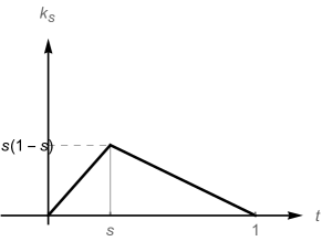
Figure 6.2. $\nu=1$, $k_{s}\left(t\right)=k\left(s,t\right)$. (A kernel function and its derivative.)

and (see Fig 6.2)

$$\frac{d}{dt}k_{s}\left(t\right) = \begin{cases}1-s&0<t\leq s\\ -s&s<t<1\end{cases}$$

$$= \left(1-s\right)\chi_{\left(0,s\right)}\left(t\right)-s\chi_{\left(s,1\right)}\left(t\right)$$

$$\left(\frac{d}{dt}\right)^{2}k_{s}\left(t\right) = -\left(1-s\right)\delta_{s}-s\delta_{s}=-\delta_{s};$$

or equivalently, $\Delta K=\delta\left(t-s\right)$, where $k$ is as in (4.3).∎

Example 4.4 (Discrete version).

Fix $R$ s.t. $0<R<1$, set $V=\mathbb{Z}_{+}$ and conductance $c_{i,i+1}=R^{-i}$. Then the energy-Hilbert space $\mathscr{H}_{R}$ consists of functions $f$ on $\mathbb{Z}_{+}$ s.t.

$$\lim_{i\rightarrow\infty}f\left(i\right)=0,\;\mbox{and}$$ (4.5)

$$\left\|f\right\|_{\mathscr{H}_{R}}^{2}=\sum_{i=1}^{\infty}\frac{1}{R^{i-1}}\left|f\left(i\right)-f\left(i-1\right)\right|^{2}<\infty,$$ (4.6)

and graph-Laplacian

$$\left(\Delta_{disc}f\right)\left(i\right)=R^{-i+1}\left(f\left(i\right)-f\left(i-1\right)\right)+R^{-i}\left(f\left(i\right)-f\left(i+1\right)\right).$$ (4.7)

In this case, the reproducing kernel $k_{R}$ is as follows:

$$k_{R}\left(i,j\right)=\left\langle v_{i}^{R},v_{j}^{R}\right\rangle_{\mathscr{H}_{R}}=\frac{R^{i\wedge j}}{1-R},\quad\forall\left(i,j\right)\in\mathbb{Z}_{+}\times\mathbb{Z}_{+}.$$ (4.8)

Here $\left(v_{i}^{R}\right)_{i\in\mathbb{Z}_{+}}$ is a system of functions in $\mathscr{H}_{R}$ such that $\left\langle v_{i}^{R},f\right\rangle_{\mathscr{H}_{R}}=f\left(i\right)$, $\forall f\in\mathscr{H}_{R}$.

Higher dimensions

Let $\Omega\subset\mathbb{R}^{\nu}$, bounded and open s.t. $\partial\Omega$ is smooth. Set

$$\begin{split}&\Delta_{0}:=-\sum_{j=1}^{\nu}\left(\frac{\partial}{\partial x_{j}}\right)^{2},\;\text{(see $\left(\ref{eq:e1}\right)$) with}\\ &dom\left(\Delta_{0}\right)=\left\{f\in L^{2}\left(\Omega\right)\>\big{|}\>\Delta f\in L^{2}\left(\Omega\right),\;\mbox{and }f\big{|}_{\partial\Omega}\equiv 0\right\}.\end{split}$$ (4.9)

We have that $\Delta_{0}$ is selfadjoint in $L^{2}\left(\Omega\right)$ and that

$$\Delta_{0}\geq 0\;\text{on $dom(\Delta_{0})$};$$ (4.10)

i.e., $\left\langle\varphi,\Delta_{0}\varphi\right\rangle_{L^{2}\left(\Omega\right)}\geq 0$, $\forall\varphi\in dom(\Delta_{0})$; and we therefore get its kernel $K$ (analogous to (4.4) in Example 4.2 (Brownian bridge).) By (4.9)-(4.10),

$$S_{t}=e^{-t\Delta_{0}}:L^{2}\left(\Omega\right)\rightarrow L^{2}\left(\Omega\right),\quad t>0$$

is a s.a. contractive semigroup.

Let

$$K=\int_{0}^{\infty}e^{-t\Delta_{0}}dt:L^{2}\left(\Omega\right)\rightarrow L^{2}\left(\Omega\right)$$ (4.11)

as an operator, generally unbounded. Since $\Delta_{0}$ is elliptic, we further get that $K$ is represented as

$$\left(Kf\right)\left(x\right)=\int_{\Omega}K\left(x,y\right)f\left(y\right)dy$$ (4.12)

where the integral in (4.12) is w.r.t. Lebesgue measure in $\mathbb{R}^{\nu}$.

Lemma 4.5.

Let $K$ be the kernel in (4.11), then

$$\Delta_{0}K=I\;\text{on $L^{2}\left(\Omega\right)$.}$$ (4.13)

Moreover, $K:\Omega\times\Omega$ is continuous, and p.d., i.e.,

$$\sum_{i}\sum_{j}\xi_{i}\xi_{j}K\left(x_{i},x_{j}\right)\geq 0$$ (4.14)

for all coefficients $\left\{\xi_{i}\right\}_{i=1}^{n}\subset\mathbb{R}$, and all $\left\{x_{i}\right\}_{i=1}^{n}\subset\Omega$.

Proof.

Let $P_{2}\left(d\lambda\right)$ denote the spectral resolution of $\Delta_{0}$ (projection valued measure (PVM)), i.e.,

$$\begin{split}&P_{2}\left(A\right)=P_{2}\left(A\right)^{*}=P_{2}\left(A\right)^{2}\\ &P_{2}\left(A\cap B\right)=P_{2}\left(A\right)P_{2}\left(B\right),\quad\forall A,B\in\mathscr{B}\left(\mathbb{R}_{+}\right),\end{split}$$ (4.15)

so that

$$\begin{split}\Delta_{0}&=\int_{0}^{\infty}\lambda P_{2}\left(d\lambda\right)\\ e^{-t\Delta_{0}}&=\int_{0}^{\infty}e^{-t\lambda}dP_{2}\left(\lambda\right),\quad t>0\end{split}$$ (4.16)

and

$$K=\int_{0}^{\infty}\frac{1}{\lambda}P_{2}\left(d\lambda\right)=\Delta_{0}^{-1}$$ (4.17)

(in general an unbounded operator.)

To see that $K$ is p.d. (see (4.14)):

Step 1. If $\varphi\in C_{c}^{\infty}\left(\Omega\right)$; then (enough to consider the real valued case)

$$\int_{\Omega}\int_{\Omega}K\left(x,y\right)\varphi\left(x\right)\varphi\left(y\right)dxdy$$

$$= \left\langle\varphi,K\varphi\right\rangle_{2}=\int_{0}^{\infty}\frac{1}{\lambda}\left\|P_{2}\left(d\lambda\right)\varphi\right\|_{2}^{2}\geq 0.$$

Step 2. Approximate $\left(\delta_{x}\right)$ with $C_{c}^{\infty}\left(\Omega\right)$. ∎

Corollary 4.6.

Let $\Delta_{0}$, and $\Omega$ be as in 4.5. Then we have a system of kernels $p_{t}\left(x,y\right)$, $t\geq 0$, $\left(x,y\right)\in\Omega\times\Omega$, such that

1. $p_{0}\left(x,y\right)=\delta_{x,y}$;

2. $p_{t}\left(x,\cdot\right)\in L^{2}\left(\Omega\right)$ for all $t\in\mathbb{R}_{+}$, $x\in\Omega$;

3. each $p_{t}\left(\cdot,\cdot\right)$ is a positive definite kernel on $\Omega\times\Omega$;

4. for $s,t\in[0,\infty)$, we have

   $$p_{s+t}\left(x,y\right)=\int_{\Omega}p_{s}\left(x,z\right)p_{t}\left(z,y\right)\,dz;\;\mbox{and}$$

5. the kernel $K$ from (4.17) satisfies

   $$K\left(x,y\right)=\int_{0}^{\infty}p_{t}\left(x,y\right)dt,\quad\forall\left(x,y\right)\in\Omega\times\Omega.$$

Proof.

Immediate from the lemma and an application of the Spectral Theorem. ∎

Remark 4.7.

The conclusions in the corollary are also valid in our discrete models, $\left(V,E,c\right)$, $E\subset V\times V\backslash\left\{\mbox{diagonal}\right\}$, and $c$ defined on $E$ as in 5.1 below. In this case,

$$\left(\Delta_{0}f\right)\left(x\right)=\sum_{\begin{subarray}{c}y\\ \left(x,y\right)\in E\end{subarray}}c_{xy}\left(f\left(x\right)-f\left(y\right)\right),\quad f\in l^{2}\left(V\right);$$ (4.18)

$$e^{-t\Delta_{0}}:l^{2}\left(V\right)\longrightarrow l^{2}\left(V\right),\quad t\in\mathbb{R}_{+};$$ (4.19)

$$\left(e^{-t\Delta_{0}}f\right)\left(x\right)=\sum_{y\in V}p_{t}\left(x,y\right)f\left(y\right),\quad\forall f\in l^{2}\left(V\right),\>t\in\mathbb{R}_{+};$$ (4.20)

and (analogous to (4) in the corollary), we have:

$$p_{s+t}\left(x,y\right)=\sum_{z\in V}p_{s}\left(x,z\right)p_{t}\left(z,y\right),\quad\forall\left(x,y\right)\in V\times V,\>\forall s,t\in[0,\infty).$$ (4.21)

Corollary 4.8.

Let $K$ be as in (4.11), then $K$ satisfies that $\Delta K=\delta\left(x-y\right)$ on $\Omega\times\Omega$, and $K\left(x,\cdot\right)\big{|}{}_{\partial\Omega}\equiv 0$.

Proof.

By well-known facts from elliptic operators, the conclusion is equivalent to (4.13).∎

Lemma 4.9.

Let $k:\Omega\times\Omega\rightarrow\mathbb{C}$ be a p.d. kernel, and let $\mathscr{H}=\mathscr{H}\left(k\right)$ be the corresponding RKHS. Then for every subset $V\subset\Omega$, $\mathscr{H}\big{|}_{V}=\left\{f\big{|}_{V}\>;\>f\in\mathscr{H}\right\}$ is a RKHS $\mathscr{H}_{V}$; and if $\varphi\in\mathscr{H}_{V}$, then $\left\|\varphi\right\|_{\mathscr{H}_{V}}=\inf\left\{\left\|f\right\|_{\mathscr{H}}\>:\>f\in\mathscr{H},\;f\big{|}_{V}=\varphi\right\}$.

Proof.

See [Aro43, Aro48]. Consider $\mathscr{H}\ominus\mathscr{N}_{V}$ (closed), where $\mathscr{N}_{V}=\left\{f\in\mathscr{H}\>;\>f\big{|}_{V}=0\right\}$. Moreover the $\inf$ is attained; $f\in\mathscr{H}$.∎

Corollary 4.10.

Let $k$, $V$, and $\mathscr{H}=\mathscr{H}\left(k\right)$ be as above. For $f\in\mathscr{H}$, write

$$f=f_{0}+f_{1}$$ (4.22)

w.r.t. the orthogonal splitting (two closed subspaces):

$$\mathscr{H}=\mathscr{N}_{V}\oplus\mathscr{N}_{V}^{\perp},\;f_{0}\in\mathscr{N}_{V},\>f_{1}\in\mathscr{N}_{V}^{\perp},$$ (4.23)

then if $\varphi\in\mathscr{H}_{V}$, we have

$$\left\|\varphi\right\|_{\mathscr{H}_{V}}=\left\|f_{1}\right\|_{\mathscr{H}},$$ (4.24)

where $\varphi=f\big{|}_{V}$.

Proof.

With the splitting (4.22), we get $f\big{|}_{V}=f_{1}\big{|}_{V}$; so

$$\varphi=f\big{|}_{V}=f_{1}\big{|}_{V},\;\mbox{and}$$ (4.25)

$$\left\|f\right\|_{\mathscr{H}}^{2}=\left\|f_{0}\right\|_{\mathscr{H}}^{2}+\left\|f_{1}\right\|_{\mathscr{H}}^{2}\geq\left\|f_{1}\right\|_{\mathscr{H}}^{2}$$

so by (4.25), $\left\|\varphi\right\|_{\mathscr{H}_{V}}=\left\|f_{1}\right\|_{\mathscr{H}}$. ∎

The purpose of the next section is to study these restrictions (discrete) in detail, from cases where $\mathscr{H}$ is one of the classical continuous RKHSs.

4.2. The Cameron-Martin space $\mathscr{H}_{CM}\left(\Omega\right)$

The Cameron–Martin Hilbert space is a RKHS (abbreviated C-M below) which gives the context for the Cameron–Martin formula which describes how abstract Wiener measure changes under translation by elements of the Cameron-Martin RKHS. Context: Abstract Wiener measure is quasi-invariant (under translation), not invariant; and the C-M RKHS serves as a tool in a formula for computing of the corresponding Radon-Nikodym derivatives, the C-H formula; see e.g., [HH93]. The technical details involved vary, depending on the dimension, and on suitable boundary conditions, see below.

Let $\Omega\subset\mathbb{R}^{\nu}$, satisfying conditions (i)-(iv); i.e., $\Omega$ is bounded, open, and connected in $\mathbb{R}^{\nu}$ with smooth boundary $\partial\Omega$.

Let $K:\Omega\times\Omega\rightarrow\mathbb{R}$ continuous, p.d., given as the Green’s function of $\Delta_{0}$, for the Dirichlet boundary condition, see (4.9). Thus, $\Delta_{0}$ is positive selfadjoint, and

$$\Delta K=\delta\left(x-y\right)\text{ on $\Omega\times\Omega$}$$ (4.26)

$$K\left(x,\cdot\right)\big{|}_{\partial\Omega}\equiv 0$$ (4.27)

see Corollary 4.8.

Let $\mathscr{H}_{CM}\left(\Omega\right)$ be the corresponding Cameron-Martin RKHS.

For $\nu=1$, $\Omega=\left(0,1\right)$, take

$$\begin{split}\mathscr{H}_{CM}\left(0,1\right)=&\Big{\{}f\>\big{|}\>f^{\prime}\in L^{2}\left(0,1\right),\;f\left(0\right)=f\left(1\right)=0,\\ &\left\|f\right\|_{CM}^{2}:=\int_{0}^{1}\left|f^{\prime}\right|^{2}dx<\infty\Big{\}}\end{split}$$ (4.28)

For $\nu>1$, let

$$\begin{split}\mathscr{H}_{CM}\left(\Omega\right)=&\left\{f\>\big{|}\>\nabla f\in L^{2}\left(\Omega\right),\>f\big{|}_{\partial\Omega}\equiv 0,\>\left\|f\right\|_{CM}^{2}:=\int_{\Omega}\left|\nabla f\right|^{2}dx<\infty\right\},\\ &\text{ where }\nabla=\left(\frac{\partial}{\partial x_{1}},\frac{\partial}{\partial x_{2}},\cdots,\frac{\partial}{\partial x_{\nu}}\right).\end{split}$$ (4.29)

Remark 4.11.

In the case of $\Omega=\left(0,1\right)$, $\nu=1$, and for $K\left(s,t\right)=s\wedge t-st$, we have $\mathscr{H}_{CM}\left(0,1\right)$ as in (4.28). The following decomposition holds:

$$K\left(s,t\right)=\sum_{n=1}^{\infty}\frac{\sin\left(n\pi s\right)\sin\left(n\pi t\right)}{\left(n\pi\right)^{2}},\quad\left(s,t\right)\in\Omega\times\Omega.$$

Proof.

Use Fourier series; or the fact that

$$\left\{\frac{\sin\left(n\pi t\right)}{n\pi}\right\}_{n=1}^{\infty}$$

is an ONB in $\mathscr{H}_{CM}\left(0,1\right)$. ∎

In general, $\nu>1$, there exists ONB $\left\{f_{n}\right\}_{n\in\mathbb{N}}$ in $\mathscr{H}_{CM}\left(\Omega\right)$ (see (4.29)), such that

$$K\left(x,y\right)=\sum_{n=1}^{\infty}f_{n}\left(x\right)f_{n}\left(y\right)\;\text{on $\Omega\times\Omega$.}$$

Proof.

A result from the theory of RKHS. ∎

Lemma 4.12 (The reproducing property).

Let $K$ be the kernel of $\Delta_{0}$ for the Dirichelet boundary condition; and let $\mathscr{H}_{CM}\left(\Omega\right)$ be the Cameron-Martin space in (4.29). Then

$$\left\langle K_{x},f\right\rangle_{CM}=f\left(x\right),\quad\forall f\in\mathscr{H}_{CM},\>\forall x\in\Omega.$$ (4.30)

Proof.

Note that

$$\mbox{LHS}{}_{\text{$\left(\ref{eq:m5}\right)$}} = \int_{\Omega}\left(\nabla K_{x}\right)\left(\nabla f\right)dy$$

$$= -\int_{\Omega}\left(\nabla^{2}K_{x}\right)f\left(y\right)dy\quad\left(\text{by \text{\text{$\left(\ref{eq:m2}\right)$,$\left(\ref{eq:m4}\right)$}}}\right)$$

$$\underset{\text{(by $\left(\ref{eq:m1}\right)$)}}{=} \int_{\Omega}\Delta K_{x}f\left(y\right)dy$$

$$\underset{\text{(by $\left(\ref{eq:m1}\right)$)}}{=} \int_{\Omega}\delta\left(x-y\right)f\left(y\right)dy=f\left(x\right);$$

where $dy=dy_{1}dy_{2}\cdots dy_{\nu}$ denotes the Lebesgue measure in $\Omega\subset\mathbb{R}^{\nu}$. ∎

We shall now consider discrete subsets:

Theorem 4.13.

Let $\Omega$, and $V\subset\Omega$, be given. Then

1. Discrete case: Fix $V\subset\Omega$, $\#V=\aleph_{0}$, where $V=\left\{x_{j}\right\}_{j=1}^{\infty}$, $x_{j}\in\Omega$. Let

   $$\mathscr{H}\left(V\right)=\text{RKHS of $K^{\left(V\right)}:=K\big{|}_{V\times V}$};$$

   then $\delta_{x_{j}}\in\mathscr{H}\left(V\right)$.

2. Continuous case; by contrast: $K_{x}^{\left(V\right)}\in\mathscr{H}_{CM}\left(V\right)$, but $\delta_{x}\notin\mathscr{H}_{CM}\left(\Omega\right)$, $x\in\Omega$.

The proof will be given in the next section.

To see that $\delta_{x}\notin\mathscr{H}_{CM}\left(\Omega\right)$, we use (4.28) when $\nu=1$, and (4.29) when $\nu>1$.

In general, by elliptic regularity, $\mathscr{H}_{CM}\left(\Omega\right)$ is a RKHS of continuous functions; and $\delta_{x}$ is not a function, so not in $\mathscr{H}_{CM}\left(\Omega\right)$.

But the RKHS of $K^{\left(V\right)}:=K\big{|}_{V\times V}$ is a discrete RKHS, and $\delta_{x}\in\mathscr{H}\left(V\right)$; proof below; 6.4.

5. Infinite network of resistors

Here we introduce a family of positive definite kernels $k:V\times V\rightarrow\mathbb{R}$, defined on infinite sets $V$ of vertices for a given graph $G=\left(V,E\right)$ with edges $E\subset V\times V\backslash(\text{diagonal})$.

There is a large literature dealing with analysis on infinite graphs; see e.g., [JP10, JP11b, JP13]; see also [OS05, BCF⁺07, CJ11].

Our main purpose here is to point out that every assignment of resistors on the edges $E$ in $G$ yields a p.d. kernel $k$, and an associated RKHS $\mathscr{H}=\mathscr{H}\left(k\right)$ such that

$$\delta_{x}\in\mathscr{H},\quad\text{for all $x\in V$.}$$ (5.1)

Definition 5.1.

Let $G=\left(V,E\right)$ be as above. Assume

1. $\left(x,y\right)\in E\Longleftrightarrow\left(y,x\right)\in E$;

2. $\exists c:E\rightarrow\mathbb{R}_{+}$ (a conductance function = 1 / resistance) such that

   1. $c_{\left(xy\right)}=c_{\left(yx\right)}$, $\forall\left(xy\right)\in E$;

   2. for all $x\in V$, $\#\left\{y\in V\>|\>c_{\left(xy\right)}>0\right\}<\infty$; and

   3. $\exists o\in V$ s.t. for $\forall x\in V\backslash\left\{o\right\}$, $\exists$ edges $\left(x_{i},x_{i+1}\right)_{0}^{n-1}\in E$ s.t. $x_{o}=0$, and $x_{n}=x$; called connectedness.

Given $G=\left(V,E\right)$, and a fixed conductance function $c:E\rightarrow\mathbb{R}_{+}$ as specified above, we now define a corresponding Laplace operator $\Delta=\Delta^{\left(c\right)}$ acting on functions on $V$, i.e., on $\mathscr{F}unc\left(V\right)$ by

$$\left(\Delta f\right)\left(x\right)=\sum_{y\sim x}c_{xy}\left(f\left(x\right)-f\left(y\right)\right).$$ (5.2)

See Fig 5.1-5.2 for examples of networks of resistors: $c_{xy}=\frac{1}{res\left(x,y\right)}$, if $\left(x,y\right)\in E$.

Figure 5.1. Examples of configuration of resistors in a network.

Figure 5.2. Example of configuration of resistors in a “large” network.

Let $\mathscr{H}$ be the Hilbert space defined as follows: A function $f$ on $V$ is in $\mathscr{H}$ iff $f\left(o\right)=0$, and

$$\left\|f\right\|_{\mathscr{H}}^{2}:=\frac{1}{2}\underset{\underset{\subset V\times V}{\left(x,y\right)\in E}}{\sum\sum}c_{xy}\left|f\left(x\right)-f\left(y\right)\right|^{2}<\infty.$$ (5.3)

Lemma 5.2 ([JP10]).

For all $x\in V\backslash\left\{o\right\}$, $\exists v_{x}\in\mathscr{H}$ s.t.

$$f\left(x\right)-f\left(o\right)=\left\langle v_{x},f\right\rangle_{\mathscr{H}},\quad\forall f\in\mathscr{H}$$ (5.4)

where

$$\left\langle h,f\right\rangle_{\mathscr{H}}=\frac{1}{2}\underset{\left(x,y\right)\in E}{\sum\sum}c_{xy}\left(\overline{h\left(x\right)}-\overline{h\left(y\right)}\right)\left(f\left(x\right)-f\left(y\right)\right),\quad\forall h,f\in\mathscr{H}.$$ (5.5)

(The system $\left\{v_{x}\right\}$ is called a system of dipoles.)

Proof.

Let $x\in V\backslash\left\{o\right\}$, and use (5.2) together with the Schwarz-inequality to show that

$$\left|f\left(x\right)-f\left(o\right)\right|^{2}\leq\sum_{i}\frac{1}{c_{x_{i}x_{i+1}}}\sum_{i}c_{x_{i}x_{i+1}}\left|f\left(x_{i}\right)-f\left(x_{i+1}\right)\right|^{2}.$$

An application of Riesz’ lemma then yields the desired conclusion.

Note that $v_{x}=v_{x}^{\left(c\right)}$ in (5.4) depends on the choice of base point $o\in V$, and on conductance function $c$; see 2.(i)-2.(ii) and (5.3). ∎

The resistance metric $R^{\left(c\right)}\left(x,y\right)=res\left(x,y\right)$ is as follows:

$$R^{\left(c\right)}\left(x,y\right) =\inf\left\{K\>:\>\left|f\left(x\right)-f\left(y\right)\right|^{2}\leq K\left\|f\right\|_{\mathscr{H}}^{2},\>\forall f\in\mathscr{H}\right\}$$

$$=\sup\left\{\left|f\left(x\right)-f\left(y\right)\right|\>:\>f\in\mathscr{H},\>\left\|f\right\|_{\mathscr{H}}\leq 1\right\}.$$

Now set

$$k^{\left(c\right)}\left(x,y\right)=\left\langle v_{x},v_{y}\right\rangle_{\mathscr{H}},\quad\forall\left(xy\right)\in\left(V\backslash\left\{o\right\}\right)\times\left(V\backslash\left\{o\right\}\right).$$ (5.6)

It follows from a theorem that $k^{\left(c\right)}$ is a Green’s function for the Laplacian $\Delta^{\left(c\right)}$ in the sense that

$$\Delta^{\left(c\right)}k^{\left(c\right)}\left(x,\cdot\right)=\delta_{x}$$ (5.7)

where the dot in (5.7) is the dummy-variable in the action. (Note that the solution to (5.7) is not unique.)

Finally, we note that

$$\Delta v_{x}=\delta_{x}-\delta_{o},\quad\forall x\in V\backslash\left\{o\right\}.$$ (5.8)

And (5.8) in turn follows from (5.4), (5.2) and a straightforward computation.

Corollary 5.3.

Let $G=\left(V,E\right)$ and conductance $c:E\rightarrow\mathbb{R}_{+}$ be as specified above. Let $\Delta=\Delta^{\left(c\right)}$ be the corresponding Laplace operator. Let $\mathscr{H}=\mathscr{H}\left(k^{c}\right)$ be the RKHS. Then

$$\left\langle\delta_{x},f\right\rangle_{\mathscr{H}}=\left(\Delta f\right)\left(x\right)$$ (5.9)

and

$$\delta_{x}=c\left(x\right)v_{x}-\sum_{y\sim x}c_{xy}v_{y}\in\mathscr{H}$$ (5.10)

holds for all $x\in V$.

Proof.

Since the system $\left\{v_{x}\right\}$ of dipoles (see (5.4)) span a dense subspace in $\mathscr{H}$, it is enough to verify (5.9) when $f=v_{y}$ for $y\in V\backslash\left\{o\right\}$. But in this case, (5.9) follows from (5.7) and a direct calculation. (For details, see [JT15].)∎

Corollary 5.4.

Let $G=\left(V,E\right)$, and conductance $c:E\rightarrow\mathbb{R}_{+}$ be as before; let $\Delta^{\left(c\right)}$ be the Laplace operator, and $\mathscr{H}_{E}^{\left(c\right)}$ the energy-Hilbert space in Definition 5.1 (see (5.3)). Let $k^{\left(c\right)}\left(x,y\right)=\left\langle v_{x},v_{y}\right\rangle_{\mathscr{H}_{E}}$ be the kernel from (5.6), i.e., the Green’s function of $\Delta^{\left(c\right)}$. Then the two Hilbert spaces $\mathscr{H}_{E}$, and $\mathscr{H}\left(k^{\left(c\right)}\right)=RKHS\left(k^{\left(c\right)}\right)$, are naturally isometrically isomorphic via $v_{x}\longmapsto k_{x}^{\left(c\right)}$ where $k_{x}^{\left(c\right)}=k^{\left(c\right)}\left(x,\cdot\right)$ for all $x\in V$.

Proof.

Let $F\in\mathscr{F}\left(V\right)$, and let $\xi$ be a function on $F$; then

$$\left\|\sum\nolimits_{x\in F}\xi\left(x\right)k_{x}^{\left(c\right)}\right\|_{\mathscr{H}\left(k^{\left(c\right)}\right)}^{2} = \underset{F\times F}{\sum\sum}\overline{\xi\left(x\right)}\xi\left(y\right)k^{\left(c\right)}\left(x,y\right)$$

$$\underset{\left(\ref{eq:g5}\right)}{=} \underset{F\times F}{\sum\sum}\overline{\xi\left(x\right)}\xi\left(y\right)\left\langle v_{x},v_{y}\right\rangle_{\mathscr{H}_{E}}$$

$$= \left\|\sum\nolimits_{x\in F}\xi\left(x\right)v_{x}\right\|_{\mathscr{H}_{E}}^{2}.$$

The remaining steps in the proof of the Corollary now follow from the standard completion from dense subspaces in the respective two Hilbert spaces $\mathscr{H}_{E}$ and $\mathscr{H}\left(k^{\left(c\right)}\right)$. ∎

In the following we show how the kernels $k^{\left(c\right)}:V\times V\rightarrow\mathbb{R}$ from (5.6) in 5.2 are related to metrics on $V$; so called resistance metrics (see, e.g., [JP10, AJSV13].)

Corollary 5.5.

Let $G=\left(V,E\right)$, and conductance $c:E\rightarrow\mathbb{R}_{+}$ be as above; and let $k^{\left(c\right)}\left(x,y\right):=\left\langle v_{x},v_{y}\right\rangle_{\mathscr{H}_{E}}$ be the corresponding Green’s function for the graph Laplacian $\Delta^{\left(c\right)}$.

Then there is a metric $R\left(=R^{\left(c\right)}=\mbox{the resistance metric}\right)$, such that

$$k^{\left(c\right)}\left(x,y\right)=\frac{R^{\left(c\right)}\left(o,x\right)+R^{\left(c\right)}\left(o,y\right)-R^{\left(c\right)}\left(x,y\right)}{2}$$ (5.11)

holds on $V\times V$. Here the base-point $o\in V$ is chosen and fixed s.t.

$$\left\langle v_{x},f\right\rangle_{\mathscr{H}_{E}}=f\left(x\right)-f\left(o\right),\quad\forall f\in\mathscr{H}_{E},\;\forall x\in V.$$ (5.12)

Proof.

See [JP10]. Set

$$R^{\left(c\right)}\left(x,y\right)=\left\|v_{x}-v_{y}\right\|_{\mathscr{H}_{E}}^{2}.$$ (5.13)

We proved in [JP10] that $R^{\left(c\right)}\left(x,y\right)$ in (5.13) indeed defines a metric on $V$; the so called resistance metric. It represents the voltage-drop from $x$ to $y$ when 1 Amp is fed into $\left(G,c\right)$ at the point $x$, and then extracted at $y$.

The verification of (5.11) is now an easy computation, as follows:

$$\frac{R^{\left(c\right)}\left(o,x\right)+R^{\left(c\right)}\left(o,y\right)-R^{\left(c\right)}\left(x,y\right)}{2}$$

$$= \frac{\left\|v_{x}\right\|_{\mathscr{H}_{E}}^{2}+\left\|v_{y}\right\|_{\mathscr{H}_{E}}^{2}-\left\|v_{x}-v_{y}\right\|_{\mathscr{H}_{E}}^{2}}{2}$$

$$= \left\langle v_{x},v_{y}\right\rangle_{\mathscr{H}_{E}}$$

$$= k^{\left(c\right)}\left(x,y\right)\quad\text{(by $\left(\ref{eq:g5}\right)$)}.$$

∎

Corollary 5.6.

The functions $R^{\left(c\right)}\left(\cdot,\cdot\right)$ which arise as in (5.11) and (5.13) are conditionally negative definite, i.e., for all finite subsets $F\subset V$ and functions $\xi$ on $F$, such that $\sum_{x\in F}\xi_{x}=0$, we have:

$$\sum_{F}\sum_{F}\overline{\xi}_{x}\xi_{y}R^{\left(c\right)}\left(x,y\right)\leq 0.$$ (5.14)

(Note that (5.14) follows from (5.13).)

Moreover, if $R^{\left(c\right)}$ arises as a restriction of a metric on $\mathbb{R}^{\nu}$, then there is a quadratic form $Q$ on $\mathbb{R}^{\nu}$ (possibly $Q=0$), and a positive measure $\mu$ on $\mathbb{R}^{\nu}$ such that

$$R^{\left(c\right)}\left(o,x\right)=Q\left(x\right)+\int_{\mathbb{R}^{\nu}}\frac{1-\cos\left(x\cdot\xi\right)}{\left|\xi\right|^{2}}d\mu\left(\xi\right),$$ (5.15)

where

$$\int_{\mathbb{R}^{\nu}}\frac{d\mu\left(\xi\right)}{1+\left|\xi\right|^{2}}<\infty.$$ (5.16)

Proof.

For details on this last point, see for example [AJV14] and [BTA04]. ∎

Proposition 5.7.

In the two cases: (i) $B\left(t\right)$, Brownian motion on $0<t<\infty$; and (ii) the Brownian bridge $B_{bri}\left(t\right)$, $0<t<1$, (see Fig 5.3) the corresponding resistance metric $R$ is as follows:

1. If $V=\left\{x_{i}\right\}_{i=1}^{\infty}\subset\left(0,\infty\right)$, $x_{1}<x_{2}<\cdots$, then

   $$R_{B}^{\left(V\right)}\left(x_{i},x_{j}\right)=\left|x_{i}-x_{j}\right|.$$ (5.17)

2. If $W=\left\{x_{i}\right\}_{i=1}^{\infty}\subset\left(0,1\right)$, $0<x_{1}<x_{2}<\cdots<1$, then

   $$R_{bridge}^{\left(W\right)}\left(x_{i},x_{j}\right)=\left|x_{i}-x_{j}\right|\cdot\left(1-\left|x_{i}-x_{j}\right|\right).$$ (5.18)

   In the completion w.r.t. the resistance metric $R_{bridge}^{\left(W\right)}$, the two endpoints $x=0$ and $x=1$ are identified; see also Fig 5.3.

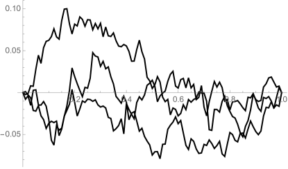
Figure 5.3. Brownian bridge $B_{bri}\left(t\right)$, a simulation of three sample paths of the Brownian bridge.

The Brownian bridge $B_{bri}\left(t\right)$ is realized on a probability space $\Omega\left(\simeq C\left(\left[0,1\right]\right)\right)$ such that $B_{bri}\left(0\right)=B_{bri}\left(1\right)=0$, and

$$\mathbb{E}\left(B_{bri}\left(s\right)B_{bri}\left(t\right)\right)=s\wedge t-st=k_{B}\left(s,t\right),$$ (5.19)

where $\mathbb{E}\left(\cdots\right)=\int_{\Omega}\cdots dP$, and $P$ denotes Wiener measure on $\Omega$.

If $\left\{B\left(t\right)\right\}_{t\in\in\left[0,1\right]}$ denotes the usual Brownian motion, $B\left(0\right)=0$, with covariance

$$\mathbb{E}\left(B\left(s\right)B\left(t\right)\right)=s\wedge t;$$ (5.20)

then we may take for $B_{bri}\left(t\right)$ as follows:

$$B_{bri}\left(t\right)=\left(1-t\right)B\left(\frac{t}{1-t}\right),\quad\forall t\in\left(0,1\right).$$ (5.21)

6. The Discrete RKHSs $\mathscr{H}\left(V\right)$ from Brownian motion

Let $V$, $K$ be as above. To get that $\delta_{x_{i}}\in\mathscr{H}\left(V\right)$, we may specify a graph $G=\left(V,E\right)$ with vertices $V$ and edges $E\subset V\times V\backslash\left\{\text{diagonal}\right\}$, and assume that, for all $x_{i}\in V$,

$$\#\left\{x_{j}\>\big{|}\>x_{i}\sim x_{j}\right\}<\infty,\quad\forall x_{i}\in V$$ (6.1)

(finite neighborhood set); see Fig 6.1. Fix a base-point $o\in V$.

Figure 6.1. $\forall i$, $\#\left\{j\>s.t.\>\left(x_{i}x_{j}\right)\in E\right\}<\infty$, every vertex $x_{i}$ has a finite set of neighbors.

Set $\mathscr{H}_{E}:=$ all functions $f$ on $V$ s.t. $f\left(o\right)=0$, with

$$\left\|f\right\|_{E}^{2}=\frac{1}{2}\underset{i\sim j}{\sum\sum}\frac{1}{res\left(i,j\right)}\left|f\left(x_{i}\right)-f\left(x_{j}\right)\right|^{2};$$

where $res\left(i,j\right)$ denotes resistance between $x_{i}$ and $x_{j}$, and

$$c_{ij}:=\frac{1}{res\left(i,j\right)}$$

is the conductance. Then $\mathscr{H}_{E}\left(G\right)$ is a RKHS for the graph $G=\left(V,E\right)$, i.e., the energy Hilbert space.

Note that

$$\widetilde{K}_{x_{i}}:=K\left(x_{i},\cdot\right)\Big{|}_{V}\in\mathscr{H}_{E}\left(G\right)$$

and

$$\left\langle\widetilde{K}_{x_{i}},f\right\rangle_{\mathscr{H}_{E}}=f\left(x_{i}\right),\quad\forall x_{i}\in V,\;\forall f\in\mathscr{H}_{E}\left(G\right).$$

Lemma 6.1.

The mapping $P_{G}:CM\left(\Omega\right)\rightarrow\mathscr{H}_{E}\left(G\right)$, $K_{x_{i}}\longmapsto\widetilde{K}_{x_{i}}$, defines a projection of the Cameron-Martin space (see (4.29)) onto $\mathscr{H}_{E}\left(G\right)$.

Proof.

Note that $J_{V}:\mathscr{H}_{E}\left(G\right)\rightarrow CM\left(\Omega\right)$, $J_{V}\widetilde{K}_{x_{j}}=K_{x_{j}}$, is an isometry. In fact, we have that

$$\left\|\sum\nolimits_{j}\xi_{j}\widetilde{K}_{x_{j}}\right\|_{\mathscr{H}_{E}\left(G\right)}^{2}=\left\|\sum\nolimits_{j}\xi_{j}K_{x_{j}}\right\|_{CM\left(\Omega\right)}^{2};$$

where $\left\|f\right\|_{CM}^{2}=\int_{\Omega}\left|\nabla f\right|^{2}dx$, for all $f\in CM\left(\Omega\right)$. Now, $P_{G}=J_{V}J_{V}^{*}$. ∎

Corollary 6.2.

$CM\left(\Omega\right)\ominus\mathscr{H}_{E}\left(G\right)=\left\{f\in CM\left(\Omega\right)\>;\>f\left(x_{j}\right)=0,\;\forall x_{j}\in V\right\}$ (See also 4.9.)

Proof.

The same as in the proof for the case of Brownian bridge:

$$\left\langle J\widetilde{K}_{x_{j}},f\right\rangle_{CM\left(\Omega\right)}=f\left(x_{j}\right),\quad\forall f\in CM\left(\Omega\right).$$

The desired result follows from this.∎

Definition 6.3.

Set

$$\begin{split}res\left(x_{i},x_{j}\right)&=R^{\left(c\right)}\left(x_{i},x_{j}\right)\\ &=\left\|K_{x_{i}}-K_{x_{j}}\right\|_{\mathscr{H}_{E}}^{2}\\ &=K\left(x_{i},x_{i}\right)+K\left(x_{j},x_{j}\right)-2K\left(x_{i},x_{j}\right)\end{split}$$ (6.2)

(We proved in [JP10] that $res\left(x_{i},x_{j}\right)$ in (6.2) indeed defines a metric on $V$; the so called resistance metric.) Let

$$\left(\Delta_{V}f\right)\left(x_{i}\right):=\sum_{x_{j}\sim x_{i}}\frac{1}{res\left(x_{i},x_{j}\right)}\left(f\left(x_{i}\right)-f\left(x_{j}\right)\right)$$

be the graph-Laplacian; where $x_{j}\sim x_{j}$ iff $\left(x_{i}x_{j}\right)\in E$.

Theorem 6.4.

Let $V\subset\Omega$ and $\Delta_{0}$, $K$, $\mathscr{H}\left(V\right)$ be as above; assume (6.1), i.e., finite neighbors in $G$. Then $\delta_{x_{i}}\in\mathscr{H}\left(V\right)$, and

$$\left(\Delta_{V}f\right)\left(x_{i}\right)=\left\langle\delta_{x_{i}},f\right\rangle_{\mathscr{H}\left(V\right)},\quad\forall f\in\mathscr{H}\left(V\right).$$

Proof.

Follows from earlier analysis. One shows that

$$\delta_{x_{i}}=\left(\sum_{x_{l}\sim x_{i}}\frac{1}{res\left(x_{i},x_{l}\right)}\right)K_{x_{i}}-\sum_{x_{j}\sim x_{i}}\frac{1}{res\left(x_{i},x_{j}\right)}K_{x_{j}}\in\mathscr{H}\left(V\right).$$

(It is a finite sum based on the assumption (6.1).)∎

Remark 6.5.

Let $\Omega\subset\mathbb{R}^{\nu}$ as above. If $\nu>1$, then the kernel $K\left(s,t\right)$, $\left(s,t\right)\in\Omega\times\Omega$, has a singularity at $x=y$, by contrast to $\nu=1$ (see below.) But we can still construct discrete graph Laplacians.

Fix $\Omega$, and let $K$ be the kernel s.t.

$$K\left(x,\cdot\right)\big{|}_{\partial\Omega}\equiv 0,\quad\forall x\in\Omega,$$

$$\Delta K=\delta\left(s,y\right)=\delta\left(x-y\right),\quad\left(x,y\right)\in\Omega\times\Omega$$

where $\Delta=-\nabla^{2}$ as a s.a. operator on $L^{2}\left(\Omega\right)$, with

$$dom\left(\Delta\right)=\left\{f\in L^{2}\left(\Omega\right)\>\big{|}\>\Delta f\in L^{2}\left(\Omega\right),\>f\big{|}_{\partial\Omega}=0\right\}.$$

So $K$ satisfies the Dirichlet boundary condition, but $K$ has a singularity at $x=y$, i.e., at the diagonal of $\Omega\times\Omega$ if $\nu>1$.

Fix $V=\left\{x_{i}\right\}_{1}^{\infty}\subset\Omega$, discrete. Fix $E\subset V\times V\backslash\left(\text{diagonal}\right)$ s.t. $\forall x_{i}\in V$, $\#\left\{j\>\big{|}\>x_{j}\sim x_{i}\right\}<\infty$, finite neighbor sets. Set

$$\left(\Delta_{V}f\right)\left(x_{i}\right)=\sum_{\underset{x_{i}\sim x_{j}}{x_{j}}}\frac{1}{res\left(x_{i},x_{j}\right)}\left(f\left(x_{i}\right)-f\left(x_{j}\right)\right)$$

and get the corresponding energy-Hilbert space

$$\mathscr{H}_{E}\left(V\right)=\left\{f\;\text{on $V$}\>\big{|}\>\underset{x_{i}\sim x_{j}}{\sum\sum}\frac{1}{res\left(x_{i},x_{j}\right)}\left|f\left(x_{i}\right)-f\left(x_{j}\right)\right|^{2}<\infty\right\}.$$

Example 6.6.

For $\nu=1$, let

$$\begin{split}&k=s\wedge t-st\\ &k_{s}\left(t\right):=k\left(s,t\right).\end{split}$$ (6.3)

Then,

$$\begin{split}k_{s}^{\prime}\left(t\right)&=\left(1-s\right)\chi_{\left[0,s\right]}\left(t\right)-s\chi_{\left[s,1\right]}\left(t\right)\\ -k_{s}^{\prime\prime}\left(t\right)&=\delta_{s}\left(t\right)=\delta_{s,t}\end{split}$$ (6.4)

Example 6.7.

For $\nu>1$, set $\Delta=-\nabla^{2}=\sum_{1}^{\nu}\left(\frac{\partial}{\partial x_{j}}\right)^{2}$, where

$$\nabla=grad=\left(\frac{\partial}{\partial x_{1}},\cdots,\frac{\partial}{\partial x_{\nu}}\right).$$ (6.5)

Set

$$\begin{split}C_{\nu}&=\begin{cases}\frac{1}{2\pi}&\nu=2\\ \frac{\nu-2}{\left|S^{\nu-1}\right|}&\nu>2\end{cases}\\ \Omega&=\left\{x\in\mathbb{R}^{\nu}\>\big{|}\>\left|x\right|<1\right\}\\ S^{\nu-1}&=\left\{x\in\mathbb{R}^{\nu}\>\big{|}\>\left|x\right|^{2}=\sum\nolimits_{j=1}^{\nu}x_{j}^{2}=1\right\}\end{split}$$ (6.6)

and, $\forall\left(x,y\right)\in\Omega\times\Omega$,

$$K\left(x,y\right)=\begin{cases}C_{\nu}\left\{\frac{1}{\left|x-y\right|^{\nu-2}}-\frac{1}{\left(\left|x\right|\left|x^{*}-y\right|\right)^{\nu-2}}\right\}&\nu>2\\ \\ \frac{1}{2\pi}\log\left(\frac{\left|x\right|\left|x^{*}-y\right|}{\left|x-y\right|}\right)&\nu=2\end{cases}$$ (6.7)

where in (6.7), we set

$$x^{*}:=\begin{cases}\frac{x}{\left|x\right|^{2}}&x\in\Omega\backslash\left\{0\right\}\\ \infty&x=0.\end{cases}$$

For $\nu=2$, see Fig 6.3.

$$D =\Omega=\left\{x\in\mathbb{R}^{\nu}\>\big{|}\>\left|x\right|<1\right\}$$

$$\partial\Omega =S^{1}=\left\{x\in\mathbb{R}^{\nu}\>\big{|}\>\left|x\right|=1\right\}$$

Figure 6.3. The case of $\nu=2$. $x\mapsto x^{*}$, reflection around $S^{1}$.

Special case of

$$K=G-\text{Poisson}\left(G\left(x,\cdot\right)\Big{|}_{\partial\Omega}\right)$$ (6.8)

where

$$G\left(x,y\right)=\begin{cases}-\frac{1}{2\pi}\log\left|x-y\right|&\nu=2\\ C_{\nu}\frac{1}{\left|x-y\right|^{\nu-2}}&\nu>2.\end{cases}\text{ (Newton potential)}$$ (6.9)

Theorem 6.8.

For $\Omega\subset\mathbb{R}^{\nu}$, bounded open, smooth boundary $\partial\Omega$, let $m_{\partial\Omega}$ be the surface measure (see [Trè06]), then $\Delta_{0}$ with boundary condition $f\big{|}_{\partial\Omega}=0$ with

$$dom\Delta_{0}=\left\{f\in L^{2}\left(\Omega\right)\>\big{|}\>\Delta f\in L^{2}\left(\Omega\right),\>f\big{|}_{\partial\Omega}=0\right\}$$

is s.a., and with $K$ as in (6.10),

$$\Delta K=\delta\left(s-y\right),\quad\left(x,y\right)\in\Omega\times\Omega$$

with $K\left(x,\cdot\right)\big{|}_{\partial\Omega}=0$, $\forall x\in\Omega$.

Proof.

For $x,y\in\Omega$, let $P_{y}$ be the Poisson kernel, and set

$$K\left(x,y\right)=G\left(x,y\right)-P_{y}\left[G\left(x,\cdot\right)\Big{|}_{\partial\Omega}\right]$$ (6.10)

view $G\left(x,\cdot\right)$ as a function on the boundary $\partial\Omega$. We have

$$P_{y}\left[G\left(x,\cdot\right)\Big{|}_{\partial\Omega}\right]=\int_{\partial\Omega}P_{y}\left(b\right)G\left(x,b\right)dm_{\partial\Omega}\left(b\right),$$

where $dm_{\partial\Omega}\left(\cdot\right)$ denotes the standard measure on the boundary $\partial\Omega$ of $\Omega$; see [Trè06].

Then

$$\Omega\ni y\longrightarrow P_{y}\left[G\left(x,\cdot\right)\Big{|}_{\partial\Omega}\right]$$

is harmonic in $\Omega$, and $\lim_{y\rightarrow b}P_{y}\left[G\left(x,\cdot\right)\Big{|}_{\partial\Omega}\right]=G\left(x,b\right)$. So, from (6.10),

$$K\left(x,b\right)=0,\quad\forall x\in\Omega,\>b\in\partial\Omega,$$

and so $K$ in (6.10) is the Dirichlet kernel. ∎

Acknowledgement.

The co-authors thank the following colleagues for helpful and enlightening discussions: Professors Daniel Alpay, Sergii Bezuglyi, Ilwoo Cho, Ka Sing Lau, Paul Muhly, Myung-Sin Song, Wayne Polyzou, Gestur Olafsson, Keri Kornelson, and members in the Math Physics seminar at the University of Iowa.

References

- [ABDdS93] Daniel Alpay, Vladimir Bolotnikov, Aad Dijksma, and Henk de Snoo, On some operator colligations and associated reproducing kernel Hilbert spaces, Operator extensions, interpolation of functions and related topics (Timişoara, 1992), Oper. Theory Adv. Appl., vol. 61, Birkhäuser, Basel, 1993, pp. 1–27. MR 1246577 (94i:47018)
- [AD92] Daniel Alpay and Harry Dym, On reproducing kernel spaces, the Schur algorithm, and interpolation in a general class of domains, Operator theory and complex analysis (Sapporo, 1991), Oper. Theory Adv. Appl., vol. 59, Birkhäuser, Basel, 1992, pp. 30–77. MR 1246809 (94j:46034)
- [AD93] by same author, On a new class of structured reproducing kernel spaces, J. Funct. Anal. 111 (1993), no. 1, 1–28. MR 1200633 (94g:46035)
- [AJ12] Daniel Alpay and Palle E. T. Jorgensen, Stochastic processes induced by singular operators, Numer. Funct. Anal. Optim. 33 (2012), no. 7-9, 708–735. MR 2966130
- [AJL11] Daniel Alpay, Palle Jorgensen, and David Levanony, A class of Gaussian processes with fractional spectral measures, J. Funct. Anal. 261 (2011), no. 2, 507–541. MR 2793121 (2012e:60101)
- [AJS14] Daniel Alpay, Palle Jorgensen, and Guy Salomon, On free stochastic processes and their derivatives, Stochastic Process. Appl. 124 (2014), no. 10, 3392–3411. MR 3231624
- [AJSV13] Daniel Alpay, Palle Jorgensen, Ron Seager, and Dan Volok, On discrete analytic functions: products, rational functions and reproducing kernels, J. Appl. Math. Comput. 41 (2013), no. 1-2, 393–426. MR 3017129
- [AJV14] Daniel Alpay, Palle Jorgensen, and Dan Volok, Relative reproducing kernel Hilbert spaces, Proc. Amer. Math. Soc. 142 (2014), no. 11, 3889–3895. MR 3251728
- [Ami78] Charles J. Amick, Some remarks on Rellich’s theorem and the Poincaré inequality, J. London Math. Soc. (2) 18 (1978), no. 1, 81–93. MR 502660 (80a:46016)
- [Aro43] N. Aronszajn, La théorie des noyaux reproduisants et ses applications. I, Proc. Cambridge Philos. Soc. 39 (1943), 133–153. MR 0008639 (5,38e)
- [Aro48] by same author, Reproducing and pseudo-reproducing kernels and their application to the partial differential equations of physics, Studies in partial differential equations. Technical report 5, preliminary note, Harvard University, Graduate School of Engineering., 1948. MR 0031663 (11,187b)
- [BCF+07] Brighid Boyle, Kristin Cekala, David Ferrone, Neil Rifkin, and Alexander Teplyaev, Electrical resistance of -gasket fractal networks, Pacific J. Math. 233 (2007), no. 1, 15–40. MR 2366367 (2010d:28006)
- [BTA04] Alain Berlinet and Christine Thomas-Agnan, Reproducing kernel Hilbert spaces in probability and statistics, Kluwer Academic Publishers, Boston, MA, 2004, With a preface by Persi Diaconis. MR 2239907 (2007b:62006)
- [CJ11] Ilwoo Cho and Palle E. T. Jorgensen, Free probability induced by electric resistance networks on energy Hilbert spaces, Opuscula Math. 31 (2011), no. 4, 549–598. MR 2823480 (2012h:05341)
- [CMPY08] Andrea Caponnetto, Charles A. Micchelli, Massimiliano Pontil, and Yiming Ying, Universal multi-task kernels, J. Mach. Learn. Res. 9 (2008), 1615–1646. MR 2426053 (2010b:68130)
- [CS02] Felipe Cucker and Steve Smale, On the mathematical foundations of learning, Bull. Amer. Math. Soc. (N.S.) 39 (2002), no. 1, 1–49 (electronic). MR 1864085 (2003a:68118)
- [DG13] Marta D’Elia and Max Gunzburger, The fractional Laplacian operator on bounded domains as a special case of the nonlocal diffusion operator, Comput. Math. Appl. 66 (2013), no. 7, 1245–1260. MR 3096457
- [DL54] J. Deny and J. L. Lions, Les espaces du type de Beppo Levi, Ann. Inst. Fourier, Grenoble 5 (1953–54), 305–370 (1955). MR 0074787 (17,646a)
- [Fer03] Xavier Fernique, Extension du théorème de Cameron-Martin aux translations aléatoires, Ann. Probab. 31 (2003), no. 3, 1296–1304. MR 1988473 (2004f:60087)
- [HH93] Takeyuki Hida and Masuyuki Hitsuda, Gaussian processes, Translations of Mathematical Monographs, vol. 120, American Mathematical Society, Providence, RI, 1993, Translated from the 1976 Japanese original by the authors. MR 1216518 (95j:60057)
- [HKL+14] S. Haeseler, M. Keller, D. Lenz, J. Masamune, and M. Schmidt, Global properties of Dirichlet forms in terms of Green’s formula, ArXiv e-prints (2014).
- [HN14] Haakan Hedenmalm and Pekka J. Nieminen, The Gaussian free field and Hadamard’s variational formula, Probab. Theory Related Fields 159 (2014), no. 1-2, 61–73. MR 3201917
- [HQKL10] Minh Ha Quang, Sung Ha Kang, and Triet M. Le, Image and video colorization using vector-valued reproducing kernel Hilbert spaces, J. Math. Imaging Vision 37 (2010), no. 1, 49–65. MR 2607639 (2011k:94032)
- [JP10] Palle E. T. Jorgensen and Erin Peter James Pearse, A Hilbert space approach to effective resistance metric, Complex Anal. Oper. Theory 4 (2010), no. 4, 975–1013. MR 2735315 (2011j:05338)
- [JP11a] Palle E. T. Jorgensen and Erin P. J. Pearse, Gel′fand triples and boundaries of infinite networks, New York J. Math. 17 (2011), 745–781. MR 2862151 (2012k:05233)
- [JP11b] by same author, Resistance boundaries of infinite networks, Random walks, boundaries and spectra, Progr. Probab., vol. 64, Birkhäuser/Springer Basel AG, Basel, 2011, pp. 111–142. MR 3051696
- [JP13] by same author, A discrete Gauss-Green identity for unbounded Laplace operators, and the transience of random walks, Israel J. Math. 196 (2013), no. 1, 113–160. MR 3096586
- [JP14] by same author, Spectral comparisons between networks with different conductance functions, J. Operator Theory 72 (2014), no. 1, 71–86. MR 3246982
- [JPT15] Palle Jorgensen, Steen Pedersen, and Feng Tian, Spectral theory of multiple intervals, Trans. Amer. Math. Soc. 367 (2015), no. 3, 1671–1735. MR 3286496
- [JT15] P. Jorgensen and F. Tian, Discrete reproducing kernel Hilbert spaces: Sampling and distribution of Dirac-masses, ArXiv e-prints (2015).
- [KH11] Sanjeev Kulkarni and Gilbert Harman, An elementary introduction to statistical learning theory, Wiley Series in Probability and Statistics, John Wiley & Sons, Inc., Hoboken, NJ, 2011. MR 2908346
- [Kre13] Christian Kreuzer, Reliable and efficient a posteriori error estimates for finite element approximations of the parabolic -Laplacian, Calcolo 50 (2013), no. 2, 79–110. MR 3049934
- [LB04] Yi Lin and Lawrence D. Brown, Statistical properties of the method of regularization with periodic Gaussian reproducing kernel, Ann. Statist. 32 (2004), no. 4, 1723–1743. MR 2089140 (2006a:62053)
- [LP11] Sneh Lata and Vern Paulsen, The Feichtinger conjecture and reproducing kernel Hilbert spaces, Indiana Univ. Math. J. 60 (2011), no. 4, 1303–1317. MR 2975345
- [Nas84] Z. Nashed, Operator parts and generalized inverses of linear manifolds with applications, Trends in theory and practice of nonlinear differential equations (Arlington, Tex., 1982), Lecture Notes in Pure and Appl. Math., vol. 90, Dekker, New York, 1984, pp. 395–412. MR 741527 (85f:47002)
- [Nel57] Edward Nelson, Kernel functions and eigenfunction expansions, Duke Math. J. 25 (1957), 15–27. MR 0091442 (19,969f)
- [NS13] M. Zuhair Nashed and Qiyu Sun, Function spaces for sampling expansions, Multiscale signal analysis and modeling, Springer, New York, 2013, pp. 81–104. MR 3024465
- [OS05] Kasso A. Okoudjou and Robert S. Strichartz, Weak uncertainty principles on fractals, J. Fourier Anal. Appl. 11 (2005), no. 3, 315–331. MR 2167172 (2006f:28011)
- [SS13] Oded Schramm and Scott Sheffield, A contour line of the continuum Gaussian free field, Probab. Theory Related Fields 157 (2013), no. 1-2, 47–80. MR 3101840
- [SZ09] Steve Smale and Ding-Xuan Zhou, Online learning with Markov sampling, Anal. Appl. (Singap.) 7 (2009), no. 1, 87–113. MR 2488871 (2010i:60021)
- [Trè06] François Trèves, Basic linear partial differential equations, Dover Publications, Inc., Mineola, NY, 2006, Reprint of the 1975 original. MR 2301309 (2007k:35004)
- [Vul13] Mirjana Vuletić, The Gaussian free field and strict plane partitions, 25th International Conference on Formal Power Series and Algebraic Combinatorics (FPSAC 2013), Discrete Math. Theor. Comput. Sci. Proc., AS, Assoc. Discrete Math. Theor. Comput. Sci., Nancy, 2013, pp. 1041–1052. MR 3091062
- [ZXZ09] Haizhang Zhang, Yuesheng Xu, and Jun Zhang, Reproducing kernel Banach spaces for machine learning, J. Mach. Learn. Res. 10 (2009), 2741–2775. MR 2579912 (2011c:62219)
- [ZXZ12] Haizhang Zhang, Yuesheng Xu, and Qinghui Zhang, Refinement of operator-valued reproducing kernels, J. Mach. Learn. Res. 13 (2012), 91–136. MR 2913695