Effects of cross-diffusion on Turing patterns in a reaction-diffusion SSmodel.

G. Gambino, S. Lupo, M. Sammartino
Abstract

In this paper the Turing pattern formation mechanism of a two component reaction-diffusion system modeling the SSchemical reaction coupled to linear cross-diffusion terms is studied. The linear cross-diffusion terms favors the destabilization of the constant steady state and the mechanism of pattern formation with respect to the standard linear diffusion case, as shown in [1]. Since the subcritical Turing bifurcations of reaction-diffusion systems lead to spontaneous onset of robust, finite-amplitude localized patterns, here a detailed investigation of the Turing pattern forming region is performed to show how the diffusion coefficients for both species (the activator and the inhibitor) influence the occurrence of supercritical or subcritical bifurcations.
The weakly nonlinear (WNL) multiple scales analysis is employed to derive the equations for the amplitude of the Turing patterns and to distinguish the supercritical and the subcritical pattern region, both in 1D and 2D domains. Numerical simulations are employed to confirm the WNL theoretical predictions through which a classification of the patterns (squares, rhombi, rectangle and hexagons) is obtained.
In particular, due to the hysteretic nature of the subcritical bifurcation, we observe the phenomenon of pattern transition from rolls to hexagons, in agreement with the bifurcation diagram.

1 Introduction

Self-organized patterning in reaction-diffusion system driven by linear diffusion has been extensively studied since the seminal paper of Turing. The interaction between diffusion and reaction has shown to yield rich and unexpected phenomena in different contexts as biological sciences, geology, geography, chemistry, industrial process, networks of electrical circuits and, of course, mathematics [2, 3, 4, 5, 6, 7, 8, 9, 10, 11, 12, 13].
In this paper the following reaction-diffusion system, firstly introduced in [1] is studied:

ut=2u+dv2v+γf(u,v),vt=d2u+du2u+γg(u,v),𝑢𝑡superscript2𝑢subscript𝑑𝑣superscript2𝑣𝛾𝑓𝑢𝑣missing-subexpressionmissing-subexpressionmissing-subexpression𝑣𝑡𝑑superscript2𝑢subscript𝑑𝑢superscript2𝑢𝛾𝑔𝑢𝑣missing-subexpression\begin{array}[]{ll}\displaystyle\frac{\partial u}{\partial t}=\nabla^{2}u+d_{v}\nabla^{2}v+\gamma f(u,v),\\ &\\ \displaystyle\frac{\partial v}{\partial t}=d\nabla^{2}u+d_{u}\nabla^{2}u+\gamma g(u,v),\end{array} (1.1)

where 2superscript2\nabla^{2} is the bidimensional Laplacian operator, d𝑑d is the ratio of the linear diffusion coefficients, dusubscript𝑑𝑢d_{u} and dvsubscript𝑑𝑣d_{v} are respectively the ratios of the cross-diffusion and the diffusion coefficients, and γ𝛾\gamma is a positive constant. The nonlinear kinetics:

f(u,v)=au+u2v,g(u,v)=bu2v,𝑓𝑢𝑣𝑎𝑢superscript𝑢2𝑣missing-subexpression𝑔𝑢𝑣𝑏superscript𝑢2𝑣missing-subexpression\begin{array}[]{ll}f(u,v)=a-u+u^{2}v,\\ g(u,v)=b-u^{2}v,\end{array} (1.2)

describe the SSchemical reaction.

We also require (1.1)-(1.2) to be equipped with the following initial conditions:

u(x,y,0)=u0(x,y),v(x,y,0)=v0(x,y),(x,y)[0,Lx]×[0,Ly],formulae-sequence𝑢𝑥𝑦0subscript𝑢0𝑥𝑦formulae-sequence𝑣𝑥𝑦0subscript𝑣0𝑥𝑦𝑥𝑦0subscript𝐿𝑥0subscript𝐿𝑦u(x,y,0)=u_{0}(x,y),\hskip 14.45377ptv(x,y,0)=v_{0}(x,y),\hskip 14.45377pt(x,y)\in\left[0,L_{x}\right]\times\left[0,L_{y}\right],

where Lxsubscript𝐿𝑥L_{x} and Lysubscript𝐿𝑦L_{y} are characteristic lengths.

Cross-diffusion, the phenomenon in which a gradient in the concentration of one species induces a flux of another species, is very significant in generating spatial structures. Recently, a large number of papers have appeared in literature, which investigate pattern formation in reaction-diffusion systems including linear and nonlinear cross-diffusion [14, 15, 16, 17, 18, 19, 20, 21, 22, 23, 24, 25, 26]. A typical example of nonlinear cross-diffusion system is the well known Shigesada-Kawasaky-Teramoto cross-diffusion system, which describes segregation effects for competing species [27]. More recently, studies on the same model have shown that cross-diffusion is the responsible of Turing instability [28, 29, 30]. In [31, 32] has been shown that linear cross-diffusion coefficients, even though they are relatively small or negative (in this last case one species tends to move in the direction of higher concentration of the other species), lead and favor pattern formation. In the above mentioned papers, the diffusion is coupled with nonlinear kinetic terms. To stress the role of cross-diffusion in pattern formation, in [33, 31] suitable cross-diffusion coefficients have been coupled to linear reaction terms and showing they are sufficient to assure pattern formation.

Madzvamuse et al. in [1] have shown that the introduction of linear cross-diffusion in the SSmodel enhances the process of pattern formation and generalizes the classical diffusion-driven instability (i.e. without cross-diffusion). In fact, in the absence of cross-diffusion terms, to obtain pattern occurrence the inhibitor must diffuse faster than the activator, d1much-greater-than𝑑1d\gg 1. When the cross-diffusion terms are involved, it is no longer necessary to choose d𝑑d much greater than one. To show the role of cross-diffusion in pattern formation, the authors in [34] choose the parameter values of the system in such a way they do not belong to the classical linear diffusion-driven instability region, but they lie on the cross-diffusion driven parameter space. In [35], sufficient conditions to guarantee the occurrence of Hopf bifurcation have been derived for the one-dimensional SSreaction-diffusion model. In [36], the occurrence of oscillating patterns due to the Hopf bifurcation is shown.
In this paper we discuss the role of the cross-diffusion coefficients into influencing the occurrence of supercritical or subcritical Turing bifurcations. In fact, pattern formation is more robust via subcritical bifurcation than via supercritical Turing instability, see [37]. When the bifurcation is supercritical, the pattern is spatially extended, it is born from zero amplitude and, it is subject to further instabilities in large domains due to the presence of different unstable modes which interact. In contrast, when the Turing bifurcation is subcritical, the arising spatial structure jumps to a finite amplitude pattern (due to the large branch amplitude into the bifurcation diagram), localized in the spatial domain, and robust to small fluctuations in the bifurcation parameter values, therefore it is more difficult to destroy the localized pattern. It is therefore important to investigate what is the mechanism which helps the subcritical Turing instability. The weakly nonlinear (WNL) multiple scales analysis is employed to derive the equations for the amplitude of the Turing patterns and to distinguish the supercritical and the subcritical pattern region. We have observed that cross-diffusion in the inhibitor component only (i.e. dusubscript𝑑𝑢d_{u}) helps the growth of the subcritical region, while the cross-diffusion in the activator component only (i.e. dvsubscript𝑑𝑣d_{v}) reduces its size.

We extend our analysis to the two-dimensional case, where the study, although much more complex, gives rise to a rich variety of super- and subcritical patterns. In particular, we recover that the case when the eigenvalue corresponding to the most unstable mode has double multiplicity and the resonance condition occurs is always subcritical. In this case we have observed the phenomenon of hexagons-rolls transition: due to the hysteretic nature of subcritical bifurcation, roll patterns lose their stability and ”jump” to hexagonal structures. Our paper is organized as follows: in Sec. 2 we perform the linear stability analysis around the uniform steady state to obtain the cross-diffusion driven instability conditions and find the corresponding Turing diffusively-driven instability parameter space. We illustrate the role of cross-diffusion and, once performed a WNL analysis, we point out how cross-diffusion coefficients influence the occurrence of supercritical or subcritical bifurcations. In addition, we show how the Stuart-Landau equation captures the behaviour of the pattern amplitude close to the marginal instability of the equilibrium P0subscript𝑃0P_{0}.
In Sec. 3 we focus on the pattern formation in a two-dimensional domain. In this case the weakly nonlinear analysis is able to predict the formation of a large number of patterns since the bifurcation can occur via a simple eigenvalue or a multiple one. On the first case, as in the one-dimensional domain, we derive the Stuart-Landau equation and the patterns emerging are squares or rolls. When the bifurcation occurs via a multiple eigenvalue - in particular with double multiplicity - more complex patterns arise, due to the interaction of different modes, such as rhombic, mixed-mode or hexagonal patterns, characterized by different amplitudes governed by a system of coupled Stuart-Landau equations. Finally, the interesting phenomenon of hysteresis is observed in correspondence od subcritical bifurcations, when different stable states for one single valued of the control parameter coexist.

2 The role of cross-diffusion in the SSmodel

First of all we perform the linear stability analysis. The unique positive steady state is given by

P0=(u0,v0)=(a+b,b(a+b)2).subscript𝑃0subscript𝑢0subscript𝑣0𝑎𝑏𝑏superscript𝑎𝑏2P_{0}=(u_{0},v_{0})=\left(a+b,\frac{b}{(a+b)^{2}}\right). (2.1)

Linearizing system (1.1)-(1.2) in the neighborhood of P0subscript𝑃0P_{0}, one gets:

w˙=J(P0)w+Dd2w,w(uu0vv0),formulae-sequence˙w𝐽subscript𝑃0wsuperscript𝐷𝑑superscript2ww𝑢subscript𝑢0𝑣subscript𝑣0\dot{\textbf{w}}=J(P_{0})\textbf{w}+D^{d}\nabla^{2}\textbf{w}\;,\qquad\qquad\textrm{}\qquad\textbf{w}\equiv\left(\begin{array}[]{c}{u-u_{0}}\\ {v-v_{0}}\end{array}\right)\;, (2.2)

where

Dd=(1dvdud)andJ(P0)=(baa+b(a+b)22ba+b(a+b)2).formulae-sequencesuperscript𝐷𝑑matrix1subscript𝑑𝑣subscript𝑑𝑢𝑑and𝐽subscript𝑃0matrix𝑏𝑎𝑎𝑏superscript𝑎𝑏22𝑏𝑎𝑏superscript𝑎𝑏2D^{d}=\begin{pmatrix}1&d_{v}\\ d_{u}&d\end{pmatrix}\qquad\mbox{and}\qquad J(P_{0})=\begin{pmatrix}\frac{b-a}{a+b}&(a+b)^{2}\\ -\frac{2b}{a+b}&-(a+b)^{2}\\ \end{pmatrix}.

In Appendix A we derived the necessary conditions for cross-diffusion driven instability:

J11+J22<0,subscript𝐽11subscript𝐽220\displaystyle J_{11}+J_{22}<0, (2.3a)
J11J22J12J21>0,subscript𝐽11subscript𝐽22subscript𝐽12subscript𝐽210\displaystyle J_{11}J_{22}-J_{12}J_{21}>0, (2.3b)
ddudv>0,𝑑subscript𝑑𝑢subscript𝑑𝑣0\displaystyle d-d_{u}d_{v}>0, (2.3c)
dJ11+J22duJ12dvJ21>0,𝑑subscript𝐽11subscript𝐽22subscript𝑑𝑢subscript𝐽12subscript𝑑𝑣subscript𝐽210\displaystyle dJ_{11}+J_{22}-d_{u}J_{12}-d_{v}J_{21}>0, (2.3d)
(dJ11+J22duJ12dvJ21)24(ddudv)(J11J22J12J21)>0,superscript𝑑subscript𝐽11subscript𝐽22subscript𝑑𝑢subscript𝐽12subscript𝑑𝑣subscript𝐽2124𝑑subscript𝑑𝑢subscript𝑑𝑣subscript𝐽11subscript𝐽22subscript𝐽12subscript𝐽210\displaystyle(dJ_{11}+J_{22}-d_{u}J_{12}-d_{v}J_{21})^{2}-4(d-d_{u}d_{v})(J_{11}J_{22}-J_{12}J_{21})>0, (2.3e)

while the critical value of the bifurcation parameter d𝑑d is:

dc=detJJ12J21+J11(dvJ21+duJ12)+2detJ(dvJ11J12)(J21duJ11)J112.subscript𝑑𝑐𝐽subscript𝐽12subscript𝐽21subscript𝐽11subscript𝑑𝑣subscript𝐽21subscript𝑑𝑢subscript𝐽122𝐽subscript𝑑𝑣subscript𝐽11subscript𝐽12subscript𝐽21subscript𝑑𝑢subscript𝐽11superscriptsubscript𝐽112d_{c}=\frac{\det J-J_{12}J_{21}+J_{11}(d_{v}J_{21}+d_{u}J_{12})+2\sqrt{\det J(d_{v}J_{11}-J_{12})(J_{21}-d_{u}J_{11})}}{J_{11}^{2}}. (2.4)

Here we study the Turing bifurcation in the presence of cross-diffusion, where the diffusive flux of a given species is also affected by the gradients of other species, and the diffusion matrix is no longer a diagonal matrix, as in the standard case. In absence of cross-diffusion, condition (2.3d) becomes dJ11+J22>0𝑑subscript𝐽11subscript𝐽220dJ_{11}+J_{22}>0. This condition together with (2.3a) leads to d>J22J11>1𝑑subscript𝐽22subscript𝐽111d>-\frac{J_{22}}{J_{11}}>1, that means:

  • (i)

    the coefficients J11subscript𝐽11J_{11} and J22subscript𝐽22J_{22} do not have the same sign (J11>0subscript𝐽110J_{11}>0 and J22<0subscript𝐽220J_{22}<0),

  • (ii)

    the diffusion coefficients of the two species are not equal and so in the absence of cross-diffusion, the inhibitor v𝑣v must diffuse faster than the activator u𝑢u.

The presence of cross diffusive effects renders the necessary conditions less restrictive: neither (i) nor (ii) need to be fulfilled.
It is important to observe that equation (2.4) corresponds to a Turing threshold condition if dcsubscript𝑑𝑐d_{c} is a real number, i.e., the discriminant detJ(dvJ11J12)(J21duJ11)𝐽subscript𝑑𝑣subscript𝐽11subscript𝐽12subscript𝐽21subscript𝑑𝑢subscript𝐽11\det J(d_{v}J_{11}-J_{12})(J_{21}-d_{u}J_{11}) is non-negative. Because of detJ>0𝐽0\det J>0, according to (2.3b), this imply that (dvJ11J12)subscript𝑑𝑣subscript𝐽11subscript𝐽12(d_{v}J_{11}-J_{12}) and (J21duJ11)subscript𝐽21subscript𝑑𝑢subscript𝐽11(J_{21}-d_{u}J_{11}) have the same sign.
In the SSmodel both of the factors are negative and so we can define the following set for the cross-diffusion coefficients:

S={(du,dv)|dv(a+b)3ba,du2bab}.𝑆conditional-setsubscript𝑑𝑢subscript𝑑𝑣formulae-sequencesubscript𝑑𝑣superscript𝑎𝑏3𝑏𝑎subscript𝑑𝑢2𝑏𝑎𝑏S=\left\{(d_{u},d_{v})|d_{v}\leq\frac{(a+b)^{3}}{b-a},d_{u}\geq\frac{2b}{a-b}\right\}. (2.5)

To emphasize the effects of cross-diffusion on the Turing instability in the SSmodel, in the following we consider the case in which one of dusubscript𝑑𝑢d_{u} and dvsubscript𝑑𝑣d_{v} are equal to zero.

Refer to caption
Refer to caption
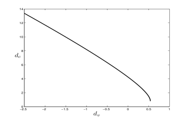
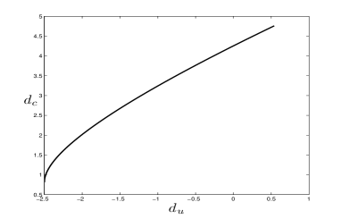
Figure 1: (a) dcsubscript𝑑𝑐d_{c} vs dvsubscript𝑑𝑣d_{v}; (b) dcsubscript𝑑𝑐d_{c} vs dusubscript𝑑𝑢d_{u}. The parameters chosen for the SSmodel are: a=0.1𝑎0.1a=0.1 and b=0.6𝑏0.6b=0.6
  • du=0subscript𝑑𝑢0d_{u}=0.
    In this case the threshold condition (2.3e) reduces to

    dc=(a+bba)2[(a+b)2+2b(a+b)+2b(a+b)2(ab)dv+22b[dv(ab)+(a+b)3].d_{c}=\left(\frac{a+b}{b-a}\right)^{2}\left[(a+b)^{2}+2b(a+b)+\frac{2b}{(a+b)^{2}}(a-b)d_{v}+2\sqrt{2b[d_{v}(a-b)+(a+b)^{3}}\right].

    The derivative of dcsubscript𝑑𝑐d_{c} with respect to dvsubscript𝑑𝑣d_{v} and evaluated at dv=0subscript𝑑𝑣0d_{v}=0, i.e., at the point corresponding to the standard Turing condition, is given by

    dcdv|dv=0=2bba2b(a+b)22b[dv(ab)+(a+b)3],evaluated-atsubscript𝑑𝑐subscript𝑑𝑣subscript𝑑𝑣02𝑏𝑏𝑎2𝑏superscript𝑎𝑏22𝑏delimited-[]subscript𝑑𝑣𝑎𝑏superscript𝑎𝑏3\frac{\partial d_{c}}{\partial d_{v}}|_{d_{v}=0}=-\frac{2b}{b-a}-\frac{2b(a+b)^{2}}{\sqrt{2b\left[d_{v}(a-b)+(a+b)^{3}\right]}},

    which is negative.
    This implies that conditions for the Turing instability in the SSmodel become more favorable, i.e., the threshold value dcsubscript𝑑𝑐d_{c} decrease as dvsubscript𝑑𝑣d_{v} increases.
    Note, however, that the Turing instability will be suppressed if the cross-diffusion coefficient becomes too large, i.e., exceeds (a+b)3basuperscript𝑎𝑏3𝑏𝑎\frac{(a+b)^{3}}{b-a}. In Fig. 1(a) we illustrate the results choosing a=0.1𝑎0.1a=0.1 and b=0.5𝑏0.5b=0.5. With this choice of the parameters we have that dvmax=0.54subscriptsubscript𝑑𝑣0.54{d_{v}}_{\max}=0.54 and dumin=2.5subscriptsubscript𝑑𝑢2.5{d_{u}}_{\min}=-2.5.

  • dv=0subscript𝑑𝑣0d_{v}=0.
    In this case the threshold condition (2.3e) reduces to

    dc=(a+bba)2[(a+b)2+2b(a+b)+du(b2a2)+2(a+b)3[2b+du(ba)]].subscript𝑑𝑐superscript𝑎𝑏𝑏𝑎2delimited-[]superscript𝑎𝑏22𝑏𝑎𝑏subscript𝑑𝑢superscript𝑏2superscript𝑎22superscript𝑎𝑏3delimited-[]2𝑏subscript𝑑𝑢𝑏𝑎d_{c}=\left(\frac{a+b}{b-a}\right)^{2}\left[(a+b)^{2}+2b(a+b)+d_{u}(b^{2}-a^{2})+2\sqrt{(a+b)^{3}[2b+d_{u}(b-a)]}\right].

    The derivative of dcsubscript𝑑𝑐d_{c} with respect to dusubscript𝑑𝑢d_{u} and evaluated at du=0subscript𝑑𝑢0d_{u}=0, i.e., at the point corresponding to the standard Turing condition, is given by

    dcdu|du=0=(a+b)3ba[1+a+b2b(a+b)],evaluated-atsubscript𝑑𝑐subscript𝑑𝑢subscript𝑑𝑢0superscript𝑎𝑏3𝑏𝑎delimited-[]1𝑎𝑏2𝑏𝑎𝑏\frac{\partial d_{c}}{\partial d_{u}}|_{d_{u}=0}=\frac{(a+b)^{3}}{b-a}\left[1+\frac{a+b}{\sqrt{2b(a+b)}}\right],

    which is positive.
    This implies that conditions for the Turing instability in the SSmodel become less favorable, i.e., the threshold value dcsubscript𝑑𝑐d_{c} increase as dusubscript𝑑𝑢d_{u} increases.
    Note, however, that the Turing instability will be suppressed if the cross-diffusion coefficient drops below 2bab2𝑏𝑎𝑏\frac{2b}{a-b}. In Fig. 1(b) we plot the dependence of the Turing threshold value dcsubscript𝑑𝑐d_{c} against the cross-diffusion coefficient dusubscript𝑑𝑢d_{u}.

Refer to caption
Refer to caption
Refer to caption
Refer to caption
Refer to caption
Refer to caption
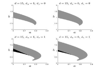
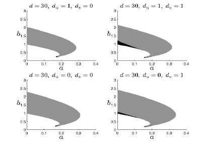
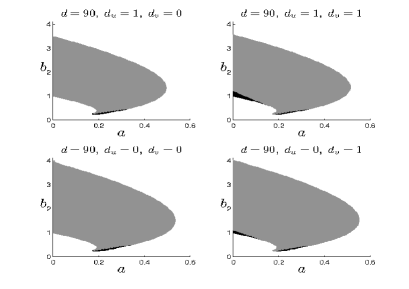
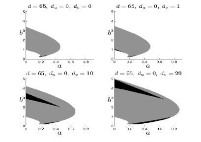
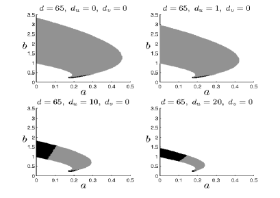
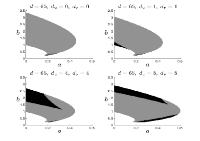
Figure 2: Turing spaces for d=15,30,65,90𝑑15306590d=15,30,65,90 in order to demonstrate the different spaces obtained.

In order to focus how cross-diffusion terms, dusubscript𝑑𝑢d_{u} and dvsubscript𝑑𝑣d_{v}, enhances the instability of the equilibrium P0subscript𝑃0P_{0}, in Fig. 2 we present some comparisons between different cases of the Turing spaces that we can summarize in the following.

  • -

    The parameter space becomes larger and larger as the value of the diffusion coefficient d𝑑d increases.

  • -

    Cross-diffusion in the inhibitor component only (dv=0subscript𝑑𝑣0d_{v}=0) produces the smallest parameter space.

  • -

    Cross-diffusion in the activator component only (du=0subscript𝑑𝑢0d_{u}=0) gives the biggest parameter space and it contains the former one.

  • -

    For some values of the bifurcation parameter d𝑑d, we obtain, in perfect agreement with the results described in [1]: the parameter space corresponding to the reaction-diffusion system without cross-diffusion (du=0subscript𝑑𝑢0d_{u}=0 and dv=0subscript𝑑𝑣0d_{v}=0) is a subspace of the Turing space corresponding to the reaction-diffusion system with cross-diffusion in both u𝑢u and v𝑣v, as is possible to see in Fig. 2(a). As d𝑑d grows this fact is not more true, in fact, as shown in Fig. 2(b) the two spaces are not included one in the other. If we increase further the value of d𝑑d we obtain the reverse situation, as shown in Fig. 2(c): the parameter space with cross-diffusion in both the components is a subspace of the parameter space without cross-diffusion.
Refer to caption
Refer to caption
Refer to caption
Refer to caption
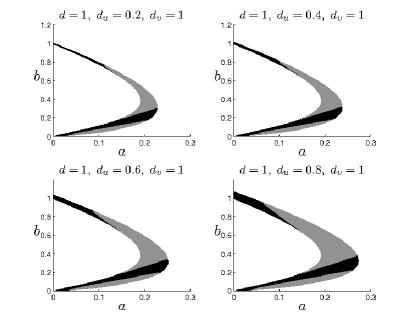
Figure 3: Turing spaces for d=1𝑑1d=1 in order to demonstrate the effect of cross-diffusion coefficients on diffusion-driven instability.

We now perform a weakly nonlinear analysis of the uniform steady state P0subscript𝑃0P_{0} when it is stable to linear homogeneous perturbations.
By expanding the solution w, the time t𝑡t and the bifurcation parameter d𝑑d, and employing the Fredholm solvability condition, we obtain the Stuart-Landau equation for the amplitude A(T)𝐴𝑇A(T):

dAdT=σALA3𝑑𝐴𝑑𝑇𝜎𝐴𝐿superscript𝐴3\frac{dA}{dT}=\sigma A-LA^{3} (2.6)

where the coefficients are obtained in terms of the parameters of the original system (1.1) and their explicit expression together with all the other details are given in Appendix B.
Depending on the sign of the coefficient L𝐿L the we distinguish the supercritical (when L>0𝐿0L>0) from the subcritical (L<0𝐿0L<0) case.
Now we can study how cross-diffusion affects the Turing region.

  • -

    As dvsubscript𝑑𝑣d_{v} increases, both the parameter space and the subcritical region increase (see Fig. 2(d)).

  • -

    As dusubscript𝑑𝑢d_{u} increases, the parameter space decreases while the subcritical region increases (see Fig. 2(e)).

  • -

    Putting du=dvsubscript𝑑𝑢subscript𝑑𝑣d_{u}=d_{v} and increasing their values, the resulting effect is an increment of the subcritical region. As regards the extension of the Turing space, because of the presence of opposite contributions, it depends, time by time, on the choice of the parameters dusubscript𝑑𝑢d_{u} and dvsubscript𝑑𝑣d_{v} (see Fig. 2(f)).

  • -

    γ𝛾\gamma plays no role in the Turing space’s representation, as it does not appear in the expressions that give the necessary conditions to destabilize the equilibrium. Moreover, γ𝛾\gamma contributes to the variation of the value of the Landau coefficient, but not of its sign; therefore, as γ𝛾\gamma varies, the region of subcriticality remains unchanged.

Observing Fig. 1(b), in contrast with standard reaction-diffusion systems where Turing instability can occur only if d>1𝑑1d>1, we note that the minimum value of the Turing threshold, attained at the boundaries of S𝑆S, is dmin=0.81subscript𝑑𝑚𝑖𝑛0.81d_{min}=0.81, i.e. a value less than 1.
In other words, we do not require short-range activation, long-range inhibition which is the standard mechanism for a diffusively-driven instability and so a Turing instability is possible even if the diffusion coefficient of the activator is larger than that of the inhibitor.
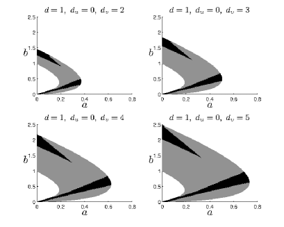
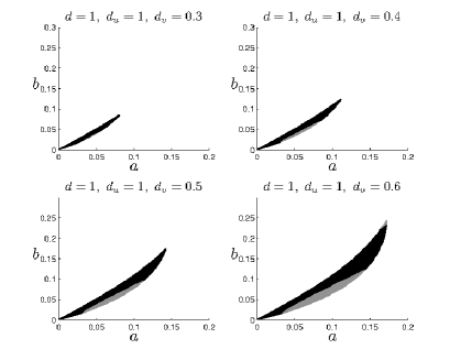
To further validate this claim in Fig. 3 we plot the parameter space when d=1𝑑1d=1 in the following cases:

  • (a)

    If d=1𝑑1d=1 and du=0subscript𝑑𝑢0d_{u}=0, the parameter space becomes larger and larger as the cross-diffusion dv𝑑𝑣dv increases (see Fig. 3(a)). In this case we have not any restrictions in the choice of dvsubscript𝑑𝑣d_{v} (provided it is positive), as the inequality ddudv>0𝑑subscript𝑑𝑢subscript𝑑𝑣0d-d_{u}d_{v}>0 is always satisfied.

  • (b)

    If d=1𝑑1d=1 and du=1subscript𝑑𝑢1d_{u}=1 we obtain the same results of the previous case (see Fig. 3(b)), but this time the inequality (2.3c) is satisfied if dv(0,1)subscript𝑑𝑣01d_{v}\in(0,1).

  • (c)

    If d=1𝑑1d=1 and dv=1subscript𝑑𝑣1d_{v}=1 we get parameter spaces that increase as dusubscript𝑑𝑢d_{u} increases in the interval (0,1)01(0,1) (see Fig. 3(c)).

(Note that we do not consider the case in which dv=0subscript𝑑𝑣0d_{v}=0, because it represents the small parameter space, as seen above, and so it would not give any relevant results, being contained in the standard Turing space.) Because of none of these spaces exist in the absence of cross-diffusion, these facts prove that a reaction-diffusion system with cross-diffusion can give rise to cross-diffusion-driven instability also putting d=1𝑑1d=1.
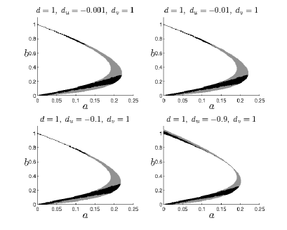
Finally we investigate the effects of negative cross-diffusion. The introduction of negative cross-diffusion in a reaction-diffusion system has already been studied in previous works. In [38], the author explains that negative cross-diffusion is a factor favoring the probability of spatial instabilities. Nevertheless, this case in quite rare, because it represents an unnatural tendency of a species moves against the concentration gradient of the other species. Recalling that when du>0subscript𝑑𝑢0d_{u}>0 one get the smallest parameter space, in Fig. 3(d) we plot the parameter spaces with d=1𝑑1d=1, dv=1subscript𝑑𝑣1d_{v}=1 and du(1,0)subscript𝑑𝑢10d_{u}\in(-1,0), to conclude that, also in this case, there are the possibility of the formation of spatial structures. In particular, we note that the parameter spaces decreases as one get values close to 11-1.

Refer to caption
Refer to caption
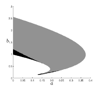
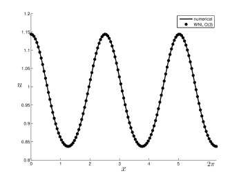
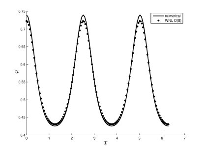
Figure 4: (a) The instability Turing region in the plane (a,b)𝑎𝑏(a,b) is shadowed: in gray the supercritical region, in black the subcritical region (see details in Section 3). The parameters are chosen as a=0.34𝑎0.34a=0.34, b=0.64𝑏0.64b=0.64, du=1subscript𝑑𝑢1d_{u}=1, dv=1𝑑𝑣1dv=1, d=45𝑑45d=45. (b) Comparison between the WNL approximated solution (dotted line) and the numerical solution of the full system (1.1) (solid line). With the choice of the parameters as above and d=dc(1+ε2)𝑑subscript𝑑𝑐1superscript𝜀2d=d_{c}(1+\varepsilon^{2}), with ε=0.2𝜀0.2\varepsilon=0.2, one has dc=43.9864subscript𝑑𝑐43.9864d_{c}=43.9864, while k¯c=2.5subscript¯𝑘𝑐2.5\bar{k}_{c}=2.5.

2.1 The Stuart-Landau equation

According to the sign of L𝐿L in (2.6), it is possible to consider the following two cases:

  1. 1.

    The supercritical case. If L>0𝐿0L>0, the Stuart-Landau equation admits a stable equilibrium solution A=σ/Lsubscript𝐴𝜎𝐿A_{\infty}=\sqrt{{\sigma}/{L}}. Assuming that only the critical wavenumber k¯¯𝑘\bar{k} is admitted in the instability interval, the long-time behavior of the solution of the reaction diffusion system (1.1) is given by 𝐰=εA𝐫cos(k¯cx)𝐰𝜀subscript𝐴𝐫subscript¯𝑘𝑐𝑥\mathbf{w}=\varepsilon A_{\infty}\operatorname{\mathbf{r}}\cos(\bar{k}_{c}x), where 𝐫𝐫\operatorname{\mathbf{r}} is defined in (B.8). Choosing the system parameters in the supercritical parameter region (see Fig. 4(a)), we compare in Fig. 4(b) the asymptotic solution predicted by the WNL analysis and the numerical solution of the system (1.1) computed via spectral methods starting from a random periodic perturbation of the constant state.

    The two solutions show a good agreement; in particular, in all the performed tests we have verified that the distance, evaluated in the L1superscript𝐿1L^{1} norm, between the WNL approximation and the numerical solution of the system is O(ε3)𝑂superscript𝜀3O(\varepsilon^{3}).

  2. 2.

    The subcritical case
    If L<0𝐿0L<0 the Stuart-Landau equation (2.6) does not admit any stable equilibrium and finite-amplitude effects tend to enhance infinitesimal disturbances growth. This is an instance of a subcritical instability and higher order terms must be considered in our WNL analysis to determine the true long-time behavior [39]. In particular, pushing the analysis up to O(ε5)𝑂superscript𝜀5O(\varepsilon^{5}), we recover the following quintic Stuart-Landau equation

    dAdT=σ¯AL¯A3+R¯A5𝑑𝐴𝑑𝑇¯𝜎𝐴¯𝐿superscript𝐴3¯𝑅superscript𝐴5\frac{dA}{dT}=\bar{\sigma}A-\bar{L}A^{3}+\bar{R}A^{5} (2.7)

    which mimics the amplitude of the pattern in the subcritical region shadowed in black in Fig. 4(a).
    Refer to caption
    Refer to caption
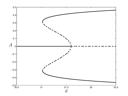
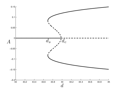
    Figure 5: (a) The bifurcation diagram in the subcritical case (the stable branches are drawn with solid line, the unstable ones with dashed line). (b) Comparison between the weakly nonlinear solution (solid line) and the numerical solution of (1.1). The parameters are chosen as: a=0.23𝑎0.23a=0.23, b=0.31𝑏0.31b=0.31, γ=76𝛾76\gamma=76, du=1subscript𝑑𝑢1d_{u}=1, dv=1subscript𝑑𝑣1d_{v}=1, and ε=0.02𝜀0.02\varepsilon=0.02; dc=43.9782subscript𝑑𝑐43.9782d_{c}=43.9782.

    The equation (2.7) predicts the long-time behavior of the amplitude of the pattern when σ¯>0¯𝜎0\bar{\sigma}>0, L¯<0¯𝐿0\bar{L}<0 and R¯<0¯𝑅0\bar{R}<0, as it admits two symmetric real stable equilibria. In Fig. 5(b) we show the comparison between the numerical and the approximated solutions predicted by the WNL. Notice that the agreement is almost rough as the amplitude is relatively insensitive to the size of the bifurcation parameter.

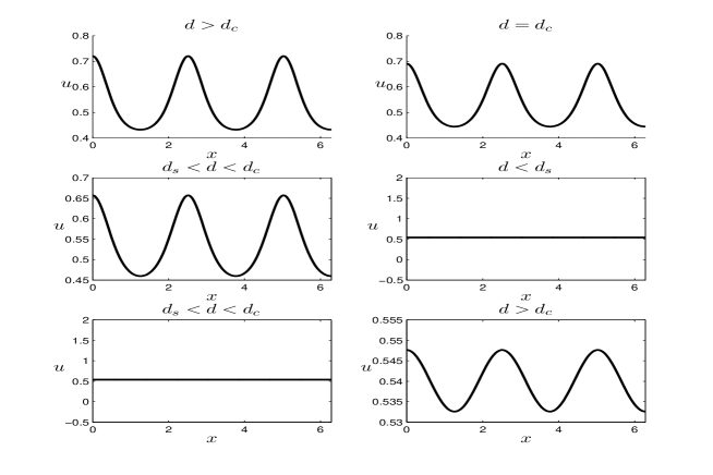
An interesting phenomenon well described by the equation (2.7) is the hysteresis, which typically emerges when qualitatively different stable states coexist (here happens in the range ds<d<dcsubscript𝑑𝑠𝑑subscript𝑑𝑐d_{s}<d<d_{c}, as it is possible to observe in Fig. 5). The hysteresis cycle in Fig. 6 shows that starting with a value of the parameter above dcsubscript𝑑𝑐d_{c} the solution stabilizes to a pattern with the amplitude corresponding to the stable branch of the bifurcation diagram. Decreasing d𝑑d below dcsubscript𝑑𝑐d_{c} the pattern does not disappear as the stable amplitude solution persists on the upper branch. Still decreasing d𝑑d below dssubscript𝑑𝑠d_{s} the pattern disappears as the amplitude solution jumps to the constant steady state. To obtain again the formation of the pattern, we have to increase the parameter d𝑑d above dcsubscript𝑑𝑐d_{c}.

Refer to caption
Figure 6: A hysteresis cycle and the corresponding pattern evolution in the subcritical case. The values of the other parameters are the same as in Fig. 5

3 Pattern formation in a two-dimensional domain

In this section our analysis will focus on the pattern formation occurrence in a rectangular domain Ω=[0,Lx]×[0,Ly]Ω0subscript𝐿𝑥0subscript𝐿𝑦\Omega=[0,L_{x}]\times[0,L_{y}]. We stress that the geometry of the domain does not affect the computation of the bifurcation value and the most unstable wavenumber, their values are still given respectively in formulas (2.4) and (A.5).

In what follows we will assume that there exists only one unstable eigenvalue λ(k¯c2)𝜆superscriptsubscript¯𝑘𝑐2\lambda(\bar{k}_{c}^{2}), admitted in the instability band. Once imposed the Neumann boundary conditions, the solution to the linear vector system (B.2), obtained via the WNL analysis at O(ε)𝑂𝜀O(\varepsilon), is given by:

𝐰1=i=1mAi(T1,T2)𝐫cos(ϕix)cos(ψiy),subscript𝐰1superscriptsubscript𝑖1𝑚subscript𝐴𝑖subscript𝑇1subscript𝑇2𝐫subscriptitalic-ϕ𝑖𝑥subscript𝜓𝑖𝑦\displaystyle{\bf w}_{1}=\sum_{i=1}^{m}A_{i}(T_{1},T_{2})\operatorname{\mathbf{r}}\cos(\phi_{i}x)\cos(\psi_{i}y), (3.1)
k¯c2=ϕi2+ψi2,whereϕipiπLx,ψiqiπLy,formulae-sequencesuperscriptsubscript¯𝑘𝑐2superscriptsubscriptitalic-ϕ𝑖2superscriptsubscript𝜓𝑖2whereformulae-sequencesubscriptitalic-ϕ𝑖subscript𝑝𝑖𝜋subscript𝐿𝑥subscript𝜓𝑖subscript𝑞𝑖𝜋subscript𝐿𝑦\displaystyle\bar{k}_{c}^{2}=\phi_{i}^{2}+\psi_{i}^{2},\ {\rm where}\ \ \phi_{i}\equiv\frac{p_{i}\pi}{L_{x}},\ \ \psi_{i}\equiv\frac{q_{i}\pi}{L_{y}}, (3.2)

where Aisubscript𝐴𝑖A_{i} are the slowly varying amplitudes, 𝐫Ker(Jk¯c2Ddc)𝐫Ker𝐽superscriptsubscript¯𝑘𝑐2superscript𝐷subscript𝑑𝑐\operatorname{\mathbf{r}}\in{\rm Ker}(J-\bar{k}_{c}^{2}D^{d_{c}}) and m𝑚m, the multiplicity, reflects the degeneracy phenomenon: in our analysis m𝑚m will take the values 111 or 222 depending on whether one or two pairs (pi,qi)subscript𝑝𝑖subscript𝑞𝑖(p_{i},q_{i}) exist such that k¯c2=ϕi2+ψi2superscriptsubscript¯𝑘𝑐2superscriptsubscriptitalic-ϕ𝑖2superscriptsubscript𝜓𝑖2\bar{k}_{c}^{2}=\phi_{i}^{2}+\psi_{i}^{2}. Once fixed the domain geometry, the types of the supported patterns strictly depend on the multiplicity.

3.1 Simple eigenvalue, m=1𝑚1m=1

When m=1𝑚1m=1 in formula (3.1), the WNL analysis traces the same steps as in one-dimensional domain and, employing the Fredholm solvability condition at O(ε3)𝑂superscript𝜀3O(\varepsilon^{3}), we still recover the Stuart-Landau equation (2.6) ruling the evolution of the pattern amplitude. Under the hypothesis that only one unstable eigenvalue λ(k¯c2)𝜆superscriptsubscript¯𝑘𝑐2\lambda(\bar{k}_{c}^{2}) is admitted in the instability band, here our investigation on the stability properties of equation (LABEL:SL_3_5) is just limited to the supercritical and the subcritical cases.

All the following numerical simulations have been performed via spectral methods employing 323232 modes both in the x𝑥x and in the y𝑦y axis. However the use of a higher number of modes in the scheme (we tested the method up to 128128128 modes) does not appreciably affect the results. The initial conditions are random periodic perturbation about P0subscript𝑃0P_{0}. Notice that, for a better presentation of the results, the amplitude of the zero mode (corresponding to the equilibrium solution) has been set equal to zero into the figures representing the spectrum of the solution. Case (1): L>0𝐿0L>0. In the supercritical case the Stuart-Landau equation admits the stable equilibrium solution A=σ/Lsubscript𝐴𝜎𝐿A_{\infty}=\sqrt{{\sigma}/{L}} and the asymptotic solution predicted by the WNL analysis is given by:

𝐰=ε𝐫Acos(ϕx)cos(ψy)+O(ε2),𝐰𝜀𝐫subscript𝐴italic-ϕ𝑥𝜓𝑦𝑂superscript𝜀2\mathbf{w}=\varepsilon\operatorname{\mathbf{r}}A_{\infty}\cos(\phi x)\cos(\psi y)+O(\varepsilon^{2}), (3.3)

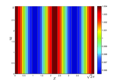
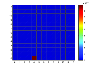
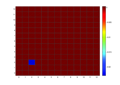
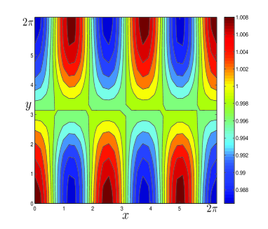
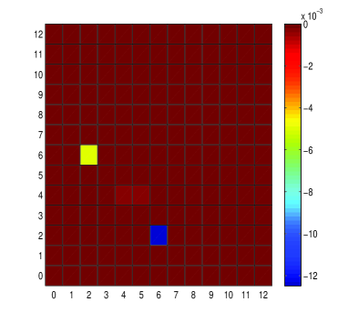
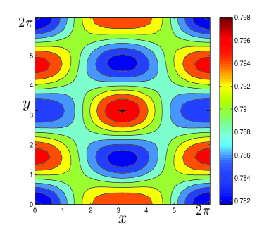
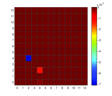
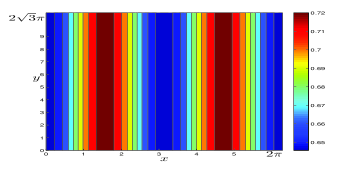
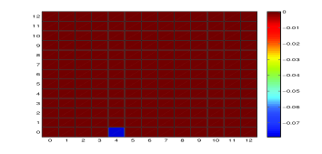
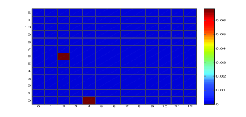
where (ϕ,ψ)italic-ϕ𝜓(\phi,\psi) is the only pair such that k¯c2=ϕ2+ψ2superscriptsubscript¯𝑘𝑐2superscriptitalic-ϕ2superscript𝜓2\bar{k}_{c}^{2}=\phi^{2}+\psi^{2}. In a rectangular domain the expected types of patterns corresponding to the solution (3.3) are rhombic pattern (see [40, 5]), whose special cases are the rolls (when ϕitalic-ϕ\phi or ψ𝜓\psi is zero) or the squares (when ϕ=ψitalic-ϕ𝜓\phi=\psi). Rolls. Choosing the system parameters as in Fig. 7 and fixing the deviation from the bifurcation value ε=0.01𝜀0.01\varepsilon=0.01, in the rectangular domain Lx=2πsubscript𝐿𝑥2𝜋L_{x}=\sqrt{2}\pi, Ly=πsubscript𝐿𝑦𝜋L_{y}=\pi the only unstable critical wavenumber is k¯c2=8superscriptsubscript¯𝑘𝑐28\bar{k}_{c}^{2}=8 and the condition (3.2) is satisfied by the unique mode pair (p,q)=(4,0)𝑝𝑞40(p,q)=(4,0). In this case the expected solution (3.3) represents a roll pattern, in good agreement with the numerical solution of the full system (1.1) shown in Fig. 7(a). In particular, the values of the most excited modes respectively of the numerical solution (shown in Fig. 7(b)) and the WNL approximated solution truncated at O(ε)𝑂𝜀O(\varepsilon) are 0.00890.00890.0089 and 0.00930.00930.0093.

Refer to caption
Refer to caption
Figure 7: Rolls. (a) The numerical solution u𝑢u of the full system (1.1). (b) Spectrum of the numerical solution. The parameters are a=0.3𝑎0.3a=0.3, b=0.7𝑏0.7b=0.7, γ=41𝛾41\gamma=41, du=1subscript𝑑𝑢1d_{u}=1, dv=1subscript𝑑𝑣1d_{v}=1, where dc=12.2643subscript𝑑𝑐12.2643d_{c}=12.2643 and ε=0.01𝜀0.01\varepsilon=0.01.

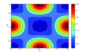
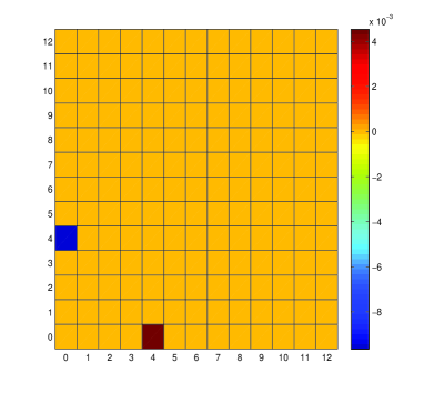
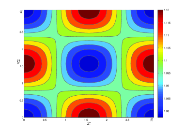
Squares. Let us choose the square domain Lx=Ly=πsubscript𝐿𝑥subscript𝐿𝑦𝜋L_{x}=L_{y}=\pi, the deviation from the bifurcation value ε=0.1𝜀0.1\varepsilon=0.1, the system parameters values as in Fig. 8. In this case the unique discrete unstable mode is k¯c2=8superscriptsubscript¯𝑘𝑐28\bar{k}_{c}^{2}=8 and the conditions in (3.2) are satisfied only by the mode pair (p,q)=(2,2)𝑝𝑞22(p,q)=(2,2). The predicted solution via the WNL analysis (3.3) is a square pattern, whose values of the amplitudes of the most excited mode (2,2)22(2,2) (computed at O(ε)𝑂𝜀O(\varepsilon) of the WNL analysis) and of the subharmonics (4,0)40(4,0), (0,4)04(0,4) and (4,4)44(4,4) (computed at O(ε2)𝑂superscript𝜀2O(\varepsilon^{2}) of the WNL analysis) are in good agreement with the corresponding amplitude modes of the numerical solution of the full system (1.1), as summarized in Table 1. The numerical solution, together with its spectrum, are given in Fig. 8.

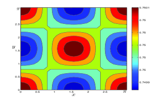
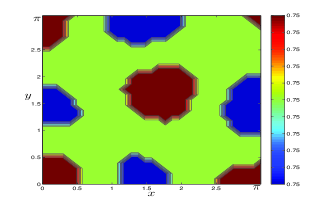
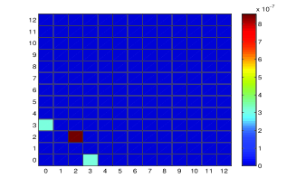
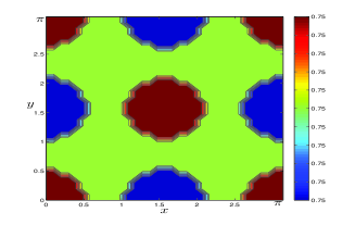
Case (2): L<0𝐿0L<0. In the subcritical case the Stuart-Landau equation (2.6) does not admit any stable equilibrium and, pushing the analysis up to O(ε5)𝑂superscript𝜀5O(\varepsilon^{5}) as in a one-dimensional domain, we recover the quintic Stuart-Landau equation (2.7). The stability properties of equation (2.7) have been already discussed in Case (2) of Section 2. The corresponding expected solution via WNL analysis is of the form (3.3), where Asubscript𝐴A_{\infty} is the stable amplitude branch predicted by the quintic Stuart-Landau (2.7). Therefore, in this case, the system still supports rhombic patterns. Here we just report a numerical experiment showing the emergence of the hysteresis phenomenon for a square pattern. We choose the domain size Lx=Ly=πsubscript𝐿𝑥subscript𝐿𝑦𝜋L_{x}=L_{y}=\pi and the system parameters as given in Fig. 9. The bifurcation diagram in Fig. 9 shows that two qualitatively different stable states coexist, therefore we expect the system supports a hysteresis cycle. Choosing the initial deviation from the bifurcation value ε=0.1𝜀0.1\varepsilon=0.1, in such a way that the unique discrete unstable mode is k¯c2=8superscriptsubscript¯𝑘𝑐28\bar{k}_{c}^{2}=8 and only the mode pair (p,q)=(2,2)𝑝𝑞22(p,q)=(2,2) satisfies the condition (3.2), the numerical simulation in the first plot of Fig.10 shows the formation of a square pattern (as predicted via WNL analysis). Following the order and the direction of the arrows in Fig. 9, the corresponding numerical simulations of the full system shows the hysteresis cycle in Fig. 10.
Refer to caption
Refer to caption
Figure 8: Squares. (a) The numerical solution u𝑢u of the full system (1.1). (b) Spectrum of the numerical solution. The parameters are a=0.3𝑎0.3a=0.3, b=0.8𝑏0.8b=0.8, γ=37𝛾37\gamma=37, du=1subscript𝑑𝑢1d_{u}=1, dv=1subscript𝑑𝑣1d_{v}=1, where dc=26.6243subscript𝑑𝑐26.6243d_{c}=26.6243 and ε=0.01𝜀0.01\varepsilon=0.01.
Modes Numerical solution Approximated solution
cos(2x)cos(2y)2𝑥2𝑦\cos(2x)\cos(2y) 0.022950.022950.02295 0.026080.026080.02608
cos(4x)4𝑥\cos(4x) 0.000230.000230.00023 0.000350.000350.00035
cos(4y)4𝑦\cos(4y) 0.000230.000230.00023 0.000350.000350.00035
cos(4x)cos(4y)4𝑥4𝑦\cos(4x)\cos(4y) 0.000050.000050.00005 0.000040.000040.00004
Table 1: Squares in the supercritical case. The parameters are chosen as in Fig. 8
Refer to caption
Figure 9: The bifurcation diagram (the stable branches are drawn with solid line and the unstable ones with dashed line). The parameters are a=0.32𝑎0.32a=0.32, b=0.76𝑏0.76b=0.76, γ=41𝛾41\gamma=41, du=1subscript𝑑𝑢1d_{u}=1, dv=1subscript𝑑𝑣1d_{v}=1, d=dc(1+ε2)𝑑subscript𝑑𝑐1superscript𝜀2d=d_{c}(1+\varepsilon^{2}), where ε=0.01𝜀0.01\varepsilon=0.01 and dc=31.5993subscript𝑑𝑐31.5993d_{c}=31.5993.
Refer to caption
Refer to caption
Refer to caption
Refer to caption
Refer to caption
Refer to caption
Refer to caption
Refer to caption
Refer to caption
Refer to caption
Figure 10: Hysteresis cycle in the subcritical case. (a) The numerical solution u𝑢u of the full system (1.1). (b) Spectrum of the numerical solution. (The parameters are chosen in Fig. 9).

3.2 Multiple eigenvalue, m=2𝑚2m=2, and the no-resonance condition holds

In this section we assume that the multiplicity of the eigenvalue λ(k¯c2)𝜆superscriptsubscript¯𝑘𝑐2\lambda(\bar{k}_{c}^{2}) is m=2𝑚2m=2 and the following no-resonance condition holds:

ϕi+ϕjϕjsubscriptitalic-ϕ𝑖subscriptitalic-ϕ𝑗subscriptitalic-ϕ𝑗\displaystyle\phi_{i}+\phi_{j}\neq\phi_{j}\quad or ψiψjψjsubscript𝜓𝑖subscript𝜓𝑗subscript𝜓𝑗\displaystyle\quad\psi_{i}-\psi_{j}\neq\psi_{j} (3.4)
and
ϕiϕjϕjsubscriptitalic-ϕ𝑖subscriptitalic-ϕ𝑗subscriptitalic-ϕ𝑗\displaystyle\phi_{i}-\phi_{j}\neq\phi_{j}\quad or ψi+ψjψjsubscript𝜓𝑖subscript𝜓𝑗subscript𝜓𝑗\displaystyle\quad\psi_{i}+\psi_{j}\neq\psi_{j}

with i,j=1,2formulae-sequence𝑖𝑗12i,j=1,2 and ij𝑖𝑗i\neq j. Performing the weakly nonlinear analysis and employing the Fredholm solvability condition at O(ε3)𝑂superscript𝜀3O(\varepsilon^{3}) to the vector system (B.4) leads to the following two coupled Landau equations for the amplitudes A1subscript𝐴1A_{1} and A2subscript𝐴2A_{2}:

dA1dT𝑑subscript𝐴1𝑑𝑇\displaystyle\frac{dA_{1}}{dT} =\displaystyle= σA1L1A13+R1A1A22,𝜎subscript𝐴1subscript𝐿1superscriptsubscript𝐴13subscript𝑅1subscript𝐴1superscriptsubscript𝐴22\displaystyle\sigma A_{1}-L_{1}A_{1}^{3}+R_{1}A_{1}A_{2}^{2}, (3.5a)
dA2dT𝑑subscript𝐴2𝑑𝑇\displaystyle\frac{dA_{2}}{dT} =\displaystyle= σA2L2A23+R2A12A2.𝜎subscript𝐴2subscript𝐿2superscriptsubscript𝐴23subscript𝑅2superscriptsubscript𝐴12subscript𝐴2\displaystyle\sigma A_{2}-L_{2}A_{2}^{3}+R_{2}A_{1}^{2}\ A_{2}. (3.5b)

All the details on the parameters of the system (3.5) are given in Appendix C. The stationary states of system (3.5) are the trivial equilibrium and the points P1±(±σL1,0)superscriptsubscript𝑃1plus-or-minusplus-or-minus𝜎subscript𝐿10P_{1}^{\pm}\equiv\left(\pm\sqrt{\frac{\sigma}{L_{1}}},0\right), P2±(0,±σL2)superscriptsubscript𝑃2plus-or-minus0plus-or-minus𝜎subscript𝐿2P_{2}^{\pm}\equiv\left(0,\pm\sqrt{\frac{\sigma}{L_{2}}}\right) and P3(±,±)(±σ(L2+R1)L1L2R1R2,±σ(L1+R2)L1L2R1R2)superscriptsubscript𝑃3plus-or-minusplus-or-minusplus-or-minus𝜎subscript𝐿2subscript𝑅1subscript𝐿1𝐿2subscript𝑅1subscript𝑅2plus-or-minus𝜎subscript𝐿1subscript𝑅2subscript𝐿1𝐿2subscript𝑅1subscript𝑅2P_{3}^{(\pm,\pm)}\equiv\left(\pm\sqrt{\frac{\sigma(L_{2}+R_{1})}{L_{1}L2-R_{1}R_{2}}},\pm\sqrt{\frac{\sigma(L_{1}+R_{2})}{L_{1}L2-R_{1}R_{2}}}\right) and their stability properties are summarized in Table 3.2.

Existence Stability
P1±superscriptsubscript𝑃1plus-or-minusP_{1}^{\pm} L1>0subscript𝐿10L_{1}>0 L1+R2<0subscript𝐿1subscript𝑅20L_{1}+R_{2}<0
P2±superscriptsubscript𝑃2plus-or-minusP_{2}^{\pm} L2>0subscript𝐿20L_{2}>0 L2+R1<0subscript𝐿2subscript𝑅10L_{2}+R_{1}<0
{L1L2R1R2<0,L1+R2<0L2+R1<0casessubscript𝐿1subscript𝐿2subscript𝑅1subscript𝑅20missing-subexpressionmissing-subexpressionsubscript𝐿1subscript𝑅20missing-subexpressionmissing-subexpressionsubscript𝐿2subscript𝑅10missing-subexpressionmissing-subexpression\left\{\begin{array}[]{lll}L_{1}L_{2}-R_{1}R_{2}<0,\\ L_{1}+R_{2}<0\\ L_{2}+R_{1}<0\end{array}\right. always unstable
P3(±,±)superscriptsubscript𝑃3plus-or-minusplus-or-minusP_{3}^{(\pm,\pm)} or
{L1L2R1R2>0,L1+R2>0L2+R1>0casessubscript𝐿1subscript𝐿2subscript𝑅1subscript𝑅20missing-subexpressionmissing-subexpressionsubscript𝐿1subscript𝑅20missing-subexpressionmissing-subexpressionsubscript𝐿2subscript𝑅10missing-subexpressionmissing-subexpression\left\{\begin{array}[]{lll}L_{1}L_{2}-R_{1}R_{2}>0,\\ L_{1}+R_{2}>0\\ L_{2}+R_{1}>0\end{array}\right. L1R1+L2R2+2L1L2<0subscript𝐿1subscript𝑅1subscript𝐿2subscript𝑅22subscript𝐿1subscript𝐿20L_{1}R_{1}+L_{2}R_{2}+2L_{1}L_{2}<0

When the system (3.5) admits at least one stable equilibrium (A1,A2)subscript𝐴1subscript𝐴2(A_{1\infty},A_{2\infty}), the long-time behavior of the solution of the reaction diffusion system (1.1) is given by:

𝐰=ε𝐫i=12Aicos(ϕix)cos(ψiy)+O(ε2).𝐰𝜀𝐫superscriptsubscript𝑖12subscript𝐴𝑖subscriptitalic-ϕ𝑖𝑥subscript𝜓𝑖𝑦𝑂superscript𝜀2\mathbf{w}=\varepsilon\operatorname{\mathbf{r}}\sum_{i=1}^{2}A_{i\infty}\cos(\phi_{i}x)\cos(\psi_{i}y)+O(\varepsilon^{2}). (3.6)

Depending on the values of (A1,A2)subscript𝐴1subscript𝐴2(A_{1\infty},A_{2\infty}) and (ϕi,ψi)subscriptitalic-ϕ𝑖subscript𝜓𝑖(\phi_{i},\psi_{i}), the solution (3.6) describes the following types of patterns:

  • (i)

    if P1±superscriptsubscript𝑃1plus-or-minusP_{1}^{\pm} or P2±superscriptsubscript𝑃2plus-or-minusP_{2}^{\pm} is stable, the solutions in (3.6) are the rhombic spatial patterns described in Section 3.1;

  • (ii)

    if P3(±,±)superscriptsubscript𝑃3plus-or-minusplus-or-minusP_{3}^{(\pm,\pm)} is stable, more complex structures arise due to the interaction of different modes ϕisubscriptitalic-ϕ𝑖\phi_{i}, ψisubscript𝜓𝑖\psi_{i}, the so-called mixed-mode patterns.

Refer to caption
Refer to caption
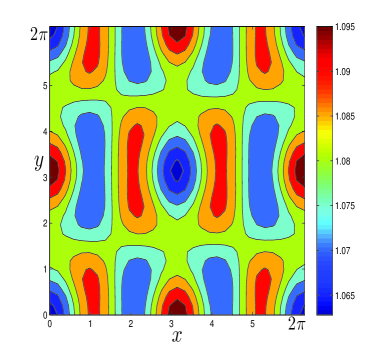
Figure 11: Rhombic pattern. Comparison between the numerical solution (a) and the weakly nonlinear first order approximation of the solution (b). The system parameters are chosen as follows: a=0.2𝑎0.2a=0.2, b=0.798𝑏0.798b=0.798, γ=21𝛾21\gamma=21, du=1subscript𝑑𝑢1d_{u}=1, dv=1subscript𝑑𝑣1d_{v}=1, where dc=11.3960subscript𝑑𝑐11.3960d_{c}=11.3960 and ε=0.1𝜀0.1\varepsilon=0.1.

In the following numerical experiments, we will show how the WNL analysis predicts different types of patterns as described in (i)-(ii) and in the simulations we fix the square domain Lx=Ly=2πsubscript𝐿𝑥subscript𝐿𝑦2𝜋L_{x}=L_{y}=2\pi. Case (i): Rhombic patterns. We choose the system parameters as in Fig. 11 and the deviation from the bifurcation values ε=0.1𝜀0.1\varepsilon=0.1. Picking up these values the only admitted unstable mode is k¯c2=6.5superscriptsubscript¯𝑘𝑐26.5\bar{k}_{c}^{2}=6.5 and the conditions in (3.2) are satisfied by the two couples (1,5)15(1,5) and (5,1)51(5,1) (for which the no-resonance conditions (3.4) hold). The only stable states of the amplitude system (3.5) are P1±superscriptsubscript𝑃1plus-or-minusP_{1}^{\pm} and P2±superscriptsubscript𝑃2plus-or-minusP_{2}^{\pm} and the predicted solution via WNL analysis (depending on the randomic initial data), respectively, the following:

𝐰=ε𝐫A1cos(2.5x)cos(0.5y)+O(ε2),or𝐰=ε𝐫A2cos(0.5x)cos(2.5y)+O(ε2),formulae-sequence𝐰𝜀𝐫subscript𝐴12.5𝑥0.5𝑦𝑂superscript𝜀2or𝐰𝜀𝐫subscript𝐴20.5𝑥2.5𝑦𝑂superscript𝜀2\begin{split}&\mathbf{w}=\varepsilon\operatorname{\mathbf{r}}A_{1\infty}\cos(2.5x)\cos(0.5y)+O(\varepsilon^{2}),\\ &\mbox{or}\\ &\mathbf{w}=\varepsilon\operatorname{\mathbf{r}}A_{2\infty}\cos(0.5x)\cos(2.5y)+O(\varepsilon^{2}),\end{split} (3.7)

where A1subscript𝐴1A_{1\infty} is the nonzero coordinate of the points P1±superscriptsubscript𝑃1plus-or-minusP_{1}^{\pm}, while A2subscript𝐴2A_{2\infty} is the nonzero coordinate of the points P2±superscriptsubscript𝑃2plus-or-minusP_{2}^{\pm}. Our numerical tests starting from a random periodic perturbation of the equilibrium show that the solution evolves to the rectangular pattern predicted in (3.7). In Fig. 11 we show the agreement (with ε=0.1𝜀0.1\varepsilon=0.1) between the numerical solution and the solution expected on the basis of the weakly nonlinear analysis.

Case (ii): Mixed-modes patterns. Let us choose the parameter values as in Fig. 12 in such a way that only the most unstable discrete mode k¯c2=10subscriptsuperscript¯𝑘2𝑐10\bar{k}^{2}_{c}=10 falls within the band of unstable modes allowed by the boundary conditions. The two mode pairs (0,5)05(0,5) and (2,3)23(2,3) satisfy the conditions (3.2) and (3.4). With this choice of the parameters the only stable equilibria of the system (3.5) are P3(±,±)superscriptsubscript𝑃3plus-or-minusplus-or-minusP_{3}^{(\pm,\pm)}, therefore the predicted long-time solution is the following mixed-mode pattern:

w=ε𝐫(A1cos(2x)cos(6y)+A2cos(6x)cos(2y))+O(ε2),w𝜀𝐫subscript𝐴12𝑥6𝑦subscript𝐴26𝑥2𝑦𝑂superscript𝜀2\textbf{w}=\varepsilon\operatorname{\mathbf{r}}\left(A_{1\infty}\cos\left(2x\right)\cos\left(6y\right)+A_{2\infty}\cos\left(6x\right)\cos\left(2y\right)\right)+O(\varepsilon^{2}), (3.8)

where A1,A2subscript𝐴1subscript𝐴2A_{1\infty},A_{2\infty} are the coordinates of the point P3(±,±)superscriptsubscript𝑃3plus-or-minusplus-or-minusP_{3}^{(\pm,\pm)}.

Refer to caption
Refer to caption
Figure 12: Mixed-modes pattern. (a) The numerical solution u𝑢u of the full system (1.1). (b) Spectrum of the numerical solution. a=0.18𝑎0.18a=0.18, b=0.901𝑏0.901b=0.901, γ=30𝛾30\gamma=30, du=1subscript𝑑𝑢1d_{u}=1, dv=1subscript𝑑𝑣1d_{v}=1, where dc=11.5168subscript𝑑𝑐11.5168d_{c}=11.5168 and ε=0.01𝜀0.01\varepsilon=0.01.

Choosing the parameter as in Fig. 12, we note a good agreement between the amplitude of the most excited modes (cos(x)cos(3y)𝑥3𝑦\cos(x)\cos(3y) and cos(3x)cos(y)3𝑥𝑦\cos(3x)\cos(y) have the same amplitude due to symmetry): 0.01250.01250.0125 and 0.01140.01140.0114 for the numerical and approximated solution, respectively.
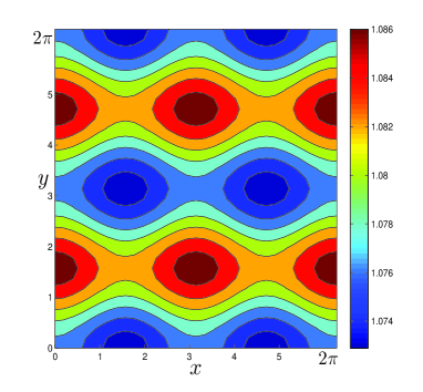
Refer to caption
Refer to caption
Figure 13: Mixed-modes pattern. (a) The numerical solution u𝑢u of the full system (1.1). (b) Spectrum of the numerical solution. a=0.18𝑎0.18a=0.18, b=0.901𝑏0.901b=0.901, γ=30𝛾30\gamma=30, du=1subscript𝑑𝑢1d_{u}=1, dv=1subscript𝑑𝑣1d_{v}=1, where dc=11.5168subscript𝑑𝑐11.5168d_{c}=11.5168 and ε=0.01𝜀0.01\varepsilon=0.01.

In another numerical test, with the choice of the parameters as in Fig. 13, the most unstable mode is k¯c2=4subscriptsuperscript¯𝑘2𝑐4\bar{k}^{2}_{c}=4 and the conditions in (3.2) are satisfied by the two couples (4,0)40(4,0) and (0,4)04(0,4). The only stable equilibria are P3(±,±)superscriptsubscript𝑃3plus-or-minusplus-or-minusP_{3}^{(\pm,\pm)} and the asymptotic solution is the following:

w=ε𝐫(A1cos(2x)+A2cos(2y))+O(ε2),w𝜀𝐫subscript𝐴12𝑥subscript𝐴22𝑦𝑂superscript𝜀2\textbf{w}=\varepsilon\operatorname{\mathbf{r}}\left(A_{1\infty}\cos(2x)+A_{2\infty}\cos(2y)\right)+O(\varepsilon^{2}), (3.9)

In Fig. 13 the numerical solution of the full system (1.1) is shown, together with its spectrum. The numerical solution is very close to the predicted WNL approximated solution, in particular the amplitude of the most unstable modes (cos(2x)2𝑥\cos(2x) and cos(2y)2𝑦\cos(2y) have the same amplitude due to symmetry) are 0.00710.00710.0071 (for the numerical solution) and 0.00780.00780.0078 (for the approximated solution).

In a further numerical test picking the parameter values as in Fig. 14, the most unstable discrete mode is exactly k¯c2=5subscriptsuperscript¯𝑘2𝑐5\bar{k}^{2}_{c}=5 and the condition (3.2) is satisfied by the two mode pairs (2,4)24(2,4) and (4,2)42(4,2). The WNL analysis predicts that the only stable equilibria are P3(±,±)superscriptsubscript𝑃3plus-or-minusplus-or-minusP_{3}^{(\pm,\pm)} and that the asymptotic solution is the following:

w=ε𝐫(A1cos(x)cos(2y)+A2cos(2x)cos(y))+O(ε2),w𝜀𝐫subscript𝐴1𝑥2𝑦subscript𝐴22𝑥𝑦𝑂superscript𝜀2\textbf{w}=\varepsilon\operatorname{\mathbf{r}}\left(A_{1\infty}\cos\left(x\right)\cos\left(2y\right)+A_{2\infty}\cos\left(2x\right)\cos\left(y\right)\right)+O(\varepsilon^{2}), (3.10)

where A1,A2subscript𝐴1subscript𝐴2A_{1\infty},A_{2\infty} are the coordinates of the point P3(±,±)superscriptsubscript𝑃3plus-or-minusplus-or-minusP_{3}^{(\pm,\pm)}. In Fig. 14 the numerical solution of the full system (1.1) is shown, together with its spectrum. The numerical solution is very close to the predicted WNL approximated solution, in particular the amplitude of the most unstable modes (cos(x)cos(2y)𝑥2𝑦\cos(x)\cos(2y) and cos(2x)cos(y)2𝑥𝑦\cos(2x)\cos(y) have the same amplitude due to symmetry) are 0.00710.00710.0071 (for the numerical solution) and 0.00720.00720.0072 (for the approximated solution).

Refer to caption
Refer to caption
Figure 14: Super-squares pattern. (a) The numerical solution u𝑢u of the full system (1.1). (b) Spectrum of the numerical solution. a=0.19𝑎0.19a=0.19, b=0.6𝑏0.6b=0.6, γ=15.3𝛾15.3\gamma=15.3, du=1subscript𝑑𝑢1d_{u}=1, dv=1subscript𝑑𝑣1d_{v}=1, where dc=6.8274subscript𝑑𝑐6.8274d_{c}=6.8274 and ε=0.1𝜀0.1\varepsilon=0.1.

3.3 Multiple eigenvalue, m=2𝑚2m=2, and the resonance condition holds

Let us assume that the multiplicity of the eigenvalue λ(k¯c2)𝜆superscriptsubscript¯𝑘𝑐2\lambda(\bar{k}_{c}^{2}) is m=2𝑚2m=2 and the following resonance conditions are satisfied:

ϕi+ϕj=ϕjsubscriptitalic-ϕ𝑖subscriptitalic-ϕ𝑗subscriptitalic-ϕ𝑗\displaystyle\phi_{i}+\phi_{j}=\phi_{j}\quad and ψiψj=ψjsubscript𝜓𝑖subscript𝜓𝑗subscript𝜓𝑗\displaystyle\quad\psi_{i}-\psi_{j}=\psi_{j} (3.11)
or
ϕiϕj=ϕjsubscriptitalic-ϕ𝑖subscriptitalic-ϕ𝑗subscriptitalic-ϕ𝑗\displaystyle\phi_{i}-\phi_{j}=\phi_{j}\quad and ψi+ψj=ψjsubscript𝜓𝑖subscript𝜓𝑗subscript𝜓𝑗\displaystyle\quad\psi_{i}+\psi_{j}=\psi_{j}

with i,j=1,2formulae-sequence𝑖𝑗12i,j=1,2 and ij𝑖𝑗i\neq j.

In what follows we hypothesize, without loss of generality, that the second condition in (3.11) holds with i=2𝑖2i=2 and j=1𝑗1j=1, therefore taking into account the relation in (3.2), we obtain ϕ2=2ϕ1subscriptitalic-ϕ22subscriptitalic-ϕ1\phi_{2}=2\phi_{1}, ψ2=0subscript𝜓20\psi_{2}=0, ψ1=3ϕ1subscript𝜓13subscriptitalic-ϕ1\psi_{1}=\sqrt{3}\phi_{1}, ϕ1=k¯c/2subscriptitalic-ϕ1subscript¯𝑘𝑐2\phi_{1}=\bar{k}_{c}/2 and also Ly=3Lxsubscript𝐿𝑦3subscript𝐿𝑥L_{y}=\sqrt{3}L_{x}. The Fredholm solvability condition on the system (B.3) at O(ε2)𝑂superscript𝜀2O(\varepsilon^{2}) allows to derive a ODEs system for the amplitudes which does not admit stable equilibrium in any parameter regimes and the WNL analysis has to be pushed to higher order, see [29]. At O(ε3)𝑂superscript𝜀3O(\varepsilon^{3}) the following system for the amplitudes A1subscript𝐴1A_{1} and A2subscript𝐴2A_{2} is found:

dA1dT=σ1A1L1A1A2+R1A13+S1A1A22,dA2dT=σ2A2L2A12+R2A23+S2A12A2,formulae-sequence𝑑subscript𝐴1𝑑𝑇subscript𝜎1subscript𝐴1subscript𝐿1subscript𝐴1subscript𝐴2subscript𝑅1superscriptsubscript𝐴13subscript𝑆1subscript𝐴1superscriptsubscript𝐴22𝑑subscript𝐴2𝑑𝑇subscript𝜎2subscript𝐴2subscript𝐿2superscriptsubscript𝐴12subscript𝑅2superscriptsubscript𝐴23subscript𝑆2superscriptsubscript𝐴12subscript𝐴2\begin{split}\frac{dA_{1}}{dT}=&\,\sigma_{1}A_{1}-L_{1}A_{1}A_{2}+R_{1}A_{1}^{3}+S_{1}A_{1}A_{2}^{2},\\ \frac{dA_{2}}{dT}=&\,\sigma_{2}A_{2}-L_{2}A_{1}^{2}+R_{2}A_{2}^{3}+S_{2}A_{1}^{2}\,A_{2},\end{split} (3.12)

where σisubscript𝜎𝑖{\sigma_{i}} and Lisubscript𝐿𝑖{L_{i}} are O(1)𝑂1O(1) perturbation of the coefficients of the amplitude equations found at O(ε2)𝑂superscript𝜀2O(\varepsilon^{2}), while Risubscript𝑅𝑖{R_{i}} and Sisubscript𝑆𝑖S_{i} are O(ε)𝑂𝜀O(\varepsilon).
In Appendix D one can find the expression of the parameters of system (3.12).
The emerging long-time solution of the full system (1.1) is approximated by:

𝐰=ε𝐫(A1cos(ϕ1x)cos(ψ1y)+A2cos(ϕ2x)cos(ψ2y))+O(ε2),𝐰𝜀𝐫subscript𝐴1subscriptitalic-ϕ1𝑥subscript𝜓1𝑦subscript𝐴2subscriptitalic-ϕ2𝑥subscript𝜓2𝑦𝑂superscript𝜀2\mathbf{w}=\varepsilon\operatorname{\mathbf{r}}(A_{1\infty}\cos(\phi_{1}x)\cos(\psi_{1}y)+A_{2\infty}\cos(\phi_{2}x)\cos(\psi_{2}y))+O(\varepsilon^{2}), (3.13)

where (A1,A2)subscript𝐴1subscript𝐴2(A_{1\infty},A_{2\infty}) is a stable state of the system (3.12).
The stability analysis of system (3.12) is almost rich and provides as stationary states the equilibria R±(0,±σ2/S2)superscript𝑅plus-or-minus0plus-or-minussubscript𝜎2subscript𝑆2R^{\pm}\equiv(0,\pm\sqrt{-{{\sigma}_{2}}/{{S}_{2}}}) and the six roots Hi±(A1i±,A2i),i=1,2,3,formulae-sequencesubscriptsuperscript𝐻plus-or-minus𝑖superscriptsubscript𝐴1𝑖plus-or-minussubscript𝐴2𝑖𝑖123H^{\pm}_{i}\equiv(A_{1i}^{\pm},A_{2i}),\ i=1,2,3, of the following system:

{A23(S1S2R1R2)+A22(L1R2+L2R1)+A2(S1σ2L1L2R2σ1)+L2σ1=0,A12=1S1(R1A22+L1A2σ1).casesotherwisesuperscriptsubscript𝐴23subscript𝑆1subscript𝑆2subscript𝑅1subscript𝑅2superscriptsubscript𝐴22subscript𝐿1subscript𝑅2subscript𝐿2subscript𝑅1subscript𝐴2subscript𝑆1subscript𝜎2subscript𝐿1subscript𝐿2subscript𝑅2subscript𝜎1subscript𝐿2subscript𝜎10otherwisesuperscriptsubscript𝐴121subscript𝑆1subscript𝑅1superscriptsubscript𝐴22subscript𝐿1subscript𝐴2subscript𝜎1\begin{cases}&A_{2}^{3}(S_{1}S_{2}-R_{1}R_{2})+A_{2}^{2}({L}_{1}R_{2}+{L}_{2}R_{1})+A_{2}\left(S_{1}{\sigma}_{2}-{L}_{1}{L}_{2}-R_{2}{\sigma}_{1}\right)+{L}_{2}{\sigma}_{1}=0,\\ &A_{1}^{2}=\displaystyle\frac{1}{S_{1}}\left(-R_{1}A_{2}^{2}\right.+\left.{L}_{1}A_{2}-{\sigma}_{1}\right).\end{cases}
Refer to caption
Refer to caption
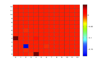
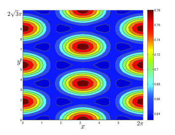
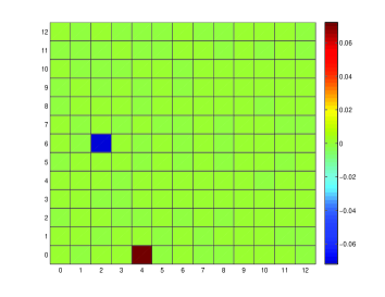
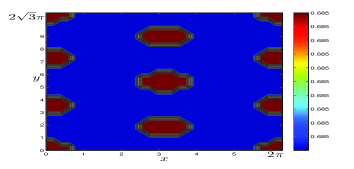
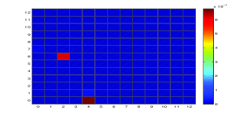
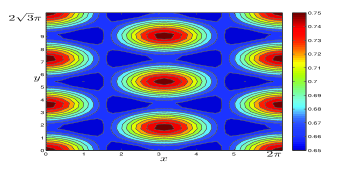
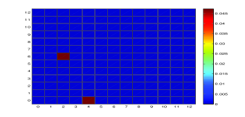
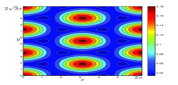
Figure 15: Hexagonal pattern. (a) The numerical solution u𝑢u of the full system (1.1). (b) Spectrum of the numerical solution. The parameters are chosen as: a=0.2𝑎0.2a=0.2, b=0.485𝑏0.485b=0.485, γ=14𝛾14\gamma=14, du=1subscript𝑑𝑢1d_{u}=1, dv=1subscript𝑑𝑣1d_{v}=1, where dc=6.7434subscript𝑑𝑐6.7434d_{c}=6.7434 and ε=0.1𝜀0.1\varepsilon=0.1.
Refer to caption
Refer to caption
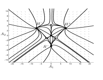
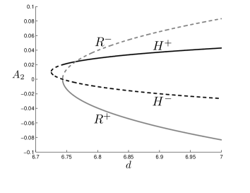
Figure 16: (a) The basin of attraction of system (3.12) and (b) the bifurcation diagram. The parameters are chosen as in Fig.15.

Whether R±superscript𝑅plus-or-minusR^{\pm} or Hi±subscriptsuperscript𝐻plus-or-minus𝑖H^{\pm}_{i} exist real and stable, the corresponding asymptotic solution (3.13) predicts respectively a roll pattern or a hexagonal pattern. In the numerical experiment shown in Fig. 15, we pick the parameters in such a way that, in the rectangular domain with Lx=2πsubscript𝐿𝑥2𝜋L_{x}=2\pi and Ly=23πsubscript𝐿𝑦23𝜋L_{y}=2\sqrt{3}\pi, the only admitted discrete unstable mode is k¯c2=4superscriptsubscript¯𝑘𝑐24\bar{k}_{c}^{2}=4.

Refer to caption
Refer to caption
Refer to caption
Refer to caption
Refer to caption
Refer to caption
Refer to caption
Refer to caption
Figure 17: Hysteresis cycle when the resonance conditions 3.11 hold. The parameters are chosen as in Fig. 15(a) The numerical solution u𝑢u of the full system (1.1). (b) Spectrum of the numerical solution.

The conditions (3.2) are satisfied by the two mode pairs (4,0)40(4,0) and (2,6)26(2,6), which also satisfy the resonance conditions (3.11). For the chosen set of parameters, the bifurcation diagram of system (3.12) in Fig. 16(b) shows a bi-stability regime of hexagonal and roll patterns, which one forms strictly depend on the initial datum.

Performing a thousand simulations, starting from different randomly chosen initial conditions, we have found that the “preferred” shape of the pattern is the hexagon shown in Fig. 15, which agrees almost well with the predicted asymptotic solution in formula (3.13). The existence of multiple stable steady states, once again, gives rise to the phenomenon of hysteresis, as shown in Fig. 17 . To obtain the roll we perform our numerical simulation of the full system (1.1) starting from an initial condition chosen in the basin of attraction of the equilibrium R+superscript𝑅R^{+}, as shown in the phase portrait of the system (3.12) in Fig. 16(a). For d<dc𝑑subscript𝑑𝑐d<d_{c} the pattern disappears because there are no stable branches. If now we increase the parameter d𝑑d above dcsubscript𝑑𝑐d_{c}, the system jumps from the rolls to the hexagons. If, instead, we come back under dcsubscript𝑑𝑐d_{c} the pattern remains always on the stable branch H+superscript𝐻H^{+}.

Appendix A Appendix

From here on we just indicate J(Pe)J𝐽subscript𝑃𝑒𝐽J(P_{e})\equiv J. Looking for solutions of system (2.2) of the form eikx+λtsuperscript𝑒𝑖𝑘𝑥𝜆𝑡e^{ikx+\lambda t} leads to the following dispersion relation, which gives the eigenvalue λ𝜆\lambda as a function of the wavenumber k𝑘k:

λ2+t(k2)λ+h(k2)=0,superscript𝜆2𝑡superscript𝑘2𝜆superscript𝑘20\lambda^{2}+t(k^{2})\lambda+h(k^{2})=0, (A.1)

where

t(k2)=k2(1+d)γtrJ,h(k2)=(ddudv)k4dγk2(dJ11+J22duJ12dvJ21)+γ2detJ.formulae-sequence𝑡superscript𝑘2superscript𝑘21𝑑𝛾tr𝐽superscript𝑘2𝑑subscript𝑑𝑢subscript𝑑𝑣superscript𝑘4𝑑𝛾superscript𝑘2𝑑subscript𝐽11subscript𝐽22subscript𝑑𝑢subscript𝐽12subscript𝑑𝑣subscript𝐽21superscript𝛾2𝐽\begin{split}t(k^{2})&=k^{2}(1+d)-\gamma\operatorname{tr}J,\\ h(k^{2})&=(d-d_{u}d_{v})k^{4}d-\gamma k^{2}(dJ_{11}+J_{22}-d_{u}J_{12}-d_{v}J_{21})+\gamma^{2}\det J.\end{split}

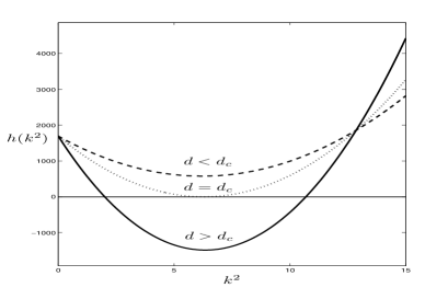
Requiring that P0subscript𝑃0P_{0} is stable to the spatially homogeneous mode k=0𝑘0k=0 entails tr(J)<0tr𝐽0{\rm tr}(J)<0 and det(J)>0det𝐽0{\rm det}(J)>0. In order to have diffusion driven instability, we require Re(λ)>0𝑅𝑒𝜆0Re(\lambda)>0 for some k0𝑘0k\neq 0, which is equivalent to impose h(k2)<0superscript𝑘20h(k^{2})<0 for some nonzero k𝑘k (see Fig. 18(a)). In order to have a upward opening parabola we require the following condition on the relationship between diffusion and cross-diffusion coefficients to hold:

det(D)=ddudv>0.𝐷𝑑subscript𝑑𝑢subscript𝑑𝑣0\det(D)=d-d_{u}d_{v}>0. (A.2)

Now, in order for h(k2)<0superscript𝑘20h(k^{2})<0 for some k2superscript𝑘2k^{2} non-zero, we require that

dJ11+J22duJ12dvJ21>0.𝑑subscript𝐽11subscript𝐽22subscript𝑑𝑢subscript𝐽12subscript𝑑𝑣subscript𝐽210dJ_{11}+J_{22}-d_{u}J_{12}-d_{v}J_{21}>0. (A.3)

Finally, for diffusively-driven instability to occur, we also require that there exists real k1,22subscriptsuperscript𝑘212k^{2}_{1,2} such that h(k1,22)=0subscriptsuperscript𝑘2120h(k^{2}_{1,2})=0 and it is easily shown this yields to impose the third and last condition for cross-diffusion-driven-instability:

(dJ11+J22duJ12dvJ21)24(ddvdu)detJ>0.superscript𝑑subscript𝐽11subscript𝐽22subscript𝑑𝑢subscript𝐽12subscript𝑑𝑣subscript𝐽2124𝑑subscript𝑑𝑣subscript𝑑𝑢𝐽0(dJ_{11}+J_{22}-d_{u}J_{12}-d_{v}J_{21})^{2}-4(d-d_{v}d_{u})\det J>0. (A.4)
Refer to caption
Refer to caption
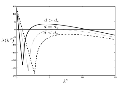
Figure 18: (a) Plot of h(k2)superscript𝑘2h(k^{2}) with fixed reaction parameter values a=0.34𝑎0.34a=0.34, b=0.64𝑏0.64b=0.64, γ=42𝛾42\gamma=42, du=1subscript𝑑𝑢1d_{u}=1, dv=1subscript𝑑𝑣1d_{v}=1. With this choice of the parameters one has dc=43.9864subscript𝑑𝑐43.9864d_{c}=43.9864, while k¯c=2.5subscript¯𝑘𝑐2.5\bar{k}_{c}=2.5. (a) Growth rate of the k𝑘k-th mode.

In Figure 4 (a), the region in the parameter space (a,b)𝑎𝑏(a,b) where the diffusion driven instability arises, and spatial patterns can develop, is given for a particular choice of the other system parameters. Notice that the minimum of h(k2)superscript𝑘2h(k^{2}) is attained when:

kc2=γdetJdcdudv,superscriptsubscript𝑘𝑐2𝛾𝐽subscript𝑑𝑐subscript𝑑𝑢subscript𝑑𝑣k_{c}^{2}=\gamma\sqrt{\frac{\det J}{d_{c}-d_{u}d_{v}}}, (A.5)

and by imposing |J|=(dJ11+J22duJ12dvJ21)24(ddvdu)𝐽superscript𝑑subscript𝐽11subscript𝐽22subscript𝑑𝑢subscript𝐽12subscript𝑑𝑣subscript𝐽2124𝑑subscript𝑑𝑣subscript𝑑𝑢|J|=\frac{(dJ_{11}+J_{22}-d_{u}J_{12}-d_{v}J_{21})^{2}}{4(d-d_{v}d_{u})} at the bifurcation, we find the bifurcation value for the diffusion parameter dcsubscript𝑑𝑐d_{c}, referred in (2.4)

For d>dc𝑑subscript𝑑𝑐d>d_{c} the eigenvalue λ(k2)𝜆superscript𝑘2\lambda(k^{2}) is positive at some k0𝑘0k\neq 0 (see Fig. 18(b)) and the system has a finite k𝑘k pattern-forming stationary instability.

Appendix B Appendix

First we expand w, the time t𝑡t and the bifurcation parameter d𝑑d as:

d=dc+εd(1)+ε2d(2)+ε3d(3)+ε4d(4)+ε5d(5)+O(ε6),𝐰=ε𝐰1+ε2𝐰2+ε3𝐰3+ε4𝐰4+ε5𝐰5+O(ε6),t=T1ε+T2ε2+T3ε3+T4ε4+T5ε5+O(ε6).formulae-sequence𝑑subscript𝑑𝑐𝜀superscript𝑑1superscript𝜀2superscript𝑑2superscript𝜀3superscript𝑑3superscript𝜀4superscript𝑑4superscript𝜀5superscript𝑑5𝑂superscript𝜀6formulae-sequence𝐰𝜀subscript𝐰1superscript𝜀2subscript𝐰2superscript𝜀3subscript𝐰3superscript𝜀4subscript𝐰4superscript𝜀5subscript𝐰5𝑂superscript𝜀6𝑡subscript𝑇1𝜀subscript𝑇2superscript𝜀2subscript𝑇3superscript𝜀3subscript𝑇4superscript𝜀4subscript𝑇5superscript𝜀5𝑂superscript𝜀6\begin{split}d&=d_{c}+\varepsilon d^{(1)}+\varepsilon^{2}d^{(2)}+\varepsilon^{3}d^{(3)}+\varepsilon^{4}d^{(4)}+\varepsilon^{5}d^{(5)}+O(\varepsilon^{6}),\\ \operatorname{\mathbf{w}}&=\varepsilon\operatorname{\mathbf{w}_{1}}+\varepsilon^{2}\operatorname{\mathbf{w}_{2}}+\varepsilon^{3}\operatorname{\mathbf{w}_{3}}+\varepsilon^{4}\operatorname{\mathbf{w}_{4}}+\varepsilon^{5}\operatorname{\mathbf{w}_{5}}+O(\varepsilon^{6}),\\ t&=\frac{T_{1}}{\varepsilon}+\frac{T_{2}}{\varepsilon^{2}}+\frac{T_{3}}{\varepsilon^{3}}+\frac{T_{4}}{\varepsilon^{4}}+\frac{T_{5}}{\varepsilon^{5}}+O(\varepsilon^{6}).\end{split} (B.1)

After substituting the above expansions into (2.2) and collecting the terms at each order in ε𝜀\varepsilon, we obtain a sequence of vector systems for the expansion coefficients wisubscriptw𝑖\textbf{w}_{i}:
O(ε)::𝑂𝜀absent\ \,O(\varepsilon):

dc𝐰1=𝟎,superscriptsubscript𝑑𝑐subscript𝐰10\mathcal{L}^{d_{c}}{\bf w}_{1}=\mathbf{0}, (B.2)

O(ε2)::𝑂superscript𝜀2absent\ \,O(\varepsilon^{2}):

dc𝐰2=𝐅,superscriptsubscript𝑑𝑐subscript𝐰2𝐅\mathcal{L}^{d_{c}}{\bf w}_{2}=\mathbf{F}, (B.3)

O(ε3)::𝑂superscript𝜀3absent\ \,O(\varepsilon^{3}):

dc𝐰3=𝐆,superscriptsubscript𝑑𝑐subscript𝐰3𝐆\mathcal{L}^{d_{c}}{\bf w}_{3}=\mathbf{G}, (B.4)

O(ε4)::𝑂superscript𝜀4absent\ \,O(\varepsilon^{4}):

dc𝐰3=𝐇,superscriptsubscript𝑑𝑐subscript𝐰3𝐇\mathcal{L}^{d_{c}}{\bf w}_{3}=\mathbf{H}, (B.5)

O(ε5)::𝑂superscript𝜀5absent\ \,O(\varepsilon^{5}):

dc𝐰3=𝐏,superscriptsubscript𝑑𝑐subscript𝐰3𝐏\mathcal{L}^{d_{c}}{\bf w}_{3}=\mathbf{P}, (B.6)

where dc=J+Ddc2superscriptsubscript𝑑𝑐𝐽superscript𝐷subscript𝑑𝑐superscript2\mathcal{L}^{d_{c}}=J+D^{d_{c}}\nabla^{2} and:

𝐅𝐅\displaystyle\mathbf{F} =\displaystyle= 𝐰1T1(000d(1))2𝐰1γ(2(a+b)u1v1+b(a+b)2u122(a+b)u1v1b(a+b)2u12),subscript𝐰1subscript𝑇1matrix000superscript𝑑1superscript2subscript𝐰1𝛾matrix2𝑎𝑏subscript𝑢1subscript𝑣1𝑏superscript𝑎𝑏2superscriptsubscript𝑢122𝑎𝑏subscript𝑢1subscript𝑣1𝑏superscript𝑎𝑏2superscriptsubscript𝑢12\displaystyle\frac{\partial\operatorname{\mathbf{w}_{1}}}{\partial T_{1}}-\begin{pmatrix}0&0\\ 0&d^{(1)}\end{pmatrix}\nabla^{2}\operatorname{\mathbf{w}_{1}}-\gamma\begin{pmatrix}2(a+b)u_{1}v_{1}+\frac{b}{(a+b)^{2}}u_{1}^{2}\\ -2(a+b)u_{1}v_{1}-\frac{b}{(a+b)^{2}}u_{1}^{2}\end{pmatrix},
𝐆𝐆\displaystyle\mathbf{G} =\displaystyle= 𝐰1T2+𝐰2T1(000d(1))2𝐰2(000d(2))2𝐰1γ(u12v1u12v1)subscript𝐰1subscript𝑇2subscript𝐰2subscript𝑇1matrix000superscript𝑑1superscript2subscript𝐰2matrix000superscript𝑑2superscript2subscript𝐰1𝛾matrixsuperscriptsubscript𝑢12subscript𝑣1superscriptsubscript𝑢12subscript𝑣1\displaystyle\frac{\partial\operatorname{\mathbf{w}_{1}}}{\partial T_{2}}+\frac{\partial\operatorname{\mathbf{w}_{2}}}{\partial T_{1}}-\begin{pmatrix}0&0\\ 0&d^{(1)}\end{pmatrix}\nabla^{2}\operatorname{\mathbf{w}_{2}}-\begin{pmatrix}0&0\\ 0&d^{(2)}\end{pmatrix}\nabla^{2}\operatorname{\mathbf{w}_{1}}-\gamma\begin{pmatrix}u_{1}^{2}v_{1}\\ -u_{1}^{2}v_{1}\end{pmatrix}
γ(2b(a+b)2u1+2(a+b)v12(a+b)u12b(a+b)2u12(a+b)v12(a+b)u1)𝐰2,𝛾matrix2𝑏superscript𝑎𝑏2subscript𝑢12𝑎𝑏subscript𝑣12𝑎𝑏subscript𝑢12𝑏superscript𝑎𝑏2subscript𝑢12𝑎𝑏subscript𝑣12𝑎𝑏subscript𝑢1subscript𝐰2\displaystyle-\gamma\begin{pmatrix}\frac{2b}{(a+b)^{2}}u_{1}+2(a+b)v_{1}&2(a+b)u_{1}\\ -\frac{2b}{(a+b)^{2}}u_{1}-2(a+b)v_{1}&-2(a+b)u_{1}\end{pmatrix}\operatorname{\mathbf{w}_{2}},
𝐇𝐇\displaystyle\mathbf{H} =\displaystyle= 𝐰1T3+𝐰2T2+𝐰3T1(000d(1))2𝐰3(000d(2))2𝐰2(000d(3))2𝐰1subscript𝐰1subscript𝑇3subscript𝐰2subscript𝑇2subscript𝐰3subscript𝑇1matrix000superscript𝑑1superscript2subscript𝐰3matrix000superscript𝑑2superscript2subscript𝐰2matrix000superscript𝑑3superscript2subscript𝐰1\displaystyle\frac{\partial\operatorname{\mathbf{w}_{1}}}{\partial T_{3}}+\frac{\partial\operatorname{\mathbf{w}_{2}}}{\partial T_{2}}+\frac{\partial\operatorname{\mathbf{w}_{3}}}{\partial T_{1}}-\begin{pmatrix}0&0\\ 0&d^{(1)}\end{pmatrix}\nabla^{2}\operatorname{\mathbf{w}_{3}}-\begin{pmatrix}0&0\\ 0&d^{(2)}\end{pmatrix}\nabla^{2}\operatorname{\mathbf{w}_{2}}-\begin{pmatrix}0&0\\ 0&d^{(3)}\end{pmatrix}\nabla^{2}\operatorname{\mathbf{w}_{1}}
γ(2b(a+b)2u1+2(a+b)v12(a+b)u12b(a+b)2u12(a+b)v12(a+b)u1)𝐰3𝛾matrix2𝑏superscript𝑎𝑏2subscript𝑢12𝑎𝑏subscript𝑣12𝑎𝑏subscript𝑢12𝑏superscript𝑎𝑏2subscript𝑢12𝑎𝑏subscript𝑣12𝑎𝑏subscript𝑢1subscript𝐰3\displaystyle-\gamma\begin{pmatrix}\frac{2b}{(a+b)^{2}}u_{1}+2(a+b)v_{1}&2(a+b)u_{1}\\ -\frac{2b}{(a+b)^{2}}u_{1}-2(a+b)v_{1}&-2(a+b)u_{1}\end{pmatrix}\operatorname{\mathbf{w}_{3}}
γ(b(a+b)2u2+2(a+b)v2+2u1v1u12b(a+b)2u22(a+b)v22u1v1u12)𝐰2,𝛾matrix𝑏superscript𝑎𝑏2subscript𝑢22𝑎𝑏subscript𝑣22subscript𝑢1subscript𝑣1superscriptsubscript𝑢12𝑏superscript𝑎𝑏2subscript𝑢22𝑎𝑏subscript𝑣22subscript𝑢1subscript𝑣1superscriptsubscript𝑢12subscript𝐰2\displaystyle-\gamma\begin{pmatrix}\frac{b}{(a+b)^{2}}u_{2}+2(a+b)v_{2}+2u_{1}v_{1}&u_{1}^{2}\\ -\frac{b}{(a+b)^{2}}u_{2}-2(a+b)v_{2}-2u_{1}v_{1}&-u_{1}^{2}\end{pmatrix}\operatorname{\mathbf{w}_{2}},
𝐏𝐏\displaystyle\mathbf{P} =\displaystyle= 𝐰1T4+𝐰2T3+𝐰3T2+𝐰4T1(000d(1))2𝐰4(000d(2))2𝐰3subscript𝐰1subscript𝑇4subscript𝐰2subscript𝑇3subscript𝐰3subscript𝑇2subscript𝐰4subscript𝑇1matrix000superscript𝑑1superscript2subscript𝐰4matrix000superscript𝑑2superscript2subscript𝐰3\displaystyle\frac{\partial\operatorname{\mathbf{w}_{1}}}{\partial T_{4}}+\frac{\partial\operatorname{\mathbf{w}_{2}}}{\partial T_{3}}+\frac{\partial\operatorname{\mathbf{w}_{3}}}{\partial T_{2}}+\frac{\partial\operatorname{\mathbf{w}_{4}}}{\partial T_{1}}-\begin{pmatrix}0&0\\ 0&d^{(1)}\end{pmatrix}\nabla^{2}\operatorname{\mathbf{w}_{4}}-\begin{pmatrix}0&0\\ 0&d^{(2)}\end{pmatrix}\nabla^{2}\operatorname{\mathbf{w}_{3}}
(000d(3))2𝐰2(000d(4))2𝐰1γ(2b(a+b)2u1+2(a+b)v12(a+b)u12b(a+b)2u12(a+b)v12(a+b)u1)𝐰4matrix000superscript𝑑3superscript2subscript𝐰2matrix000superscript𝑑4superscript2subscript𝐰1𝛾matrix2𝑏superscript𝑎𝑏2subscript𝑢12𝑎𝑏subscript𝑣12𝑎𝑏subscript𝑢12𝑏superscript𝑎𝑏2subscript𝑢12𝑎𝑏subscript𝑣12𝑎𝑏subscript𝑢1subscript𝐰4\displaystyle-\begin{pmatrix}0&0\\ 0&d^{(3)}\end{pmatrix}\nabla^{2}\operatorname{\mathbf{w}_{2}}-\begin{pmatrix}0&0\\ 0&d^{(4)}\end{pmatrix}\nabla^{2}\operatorname{\mathbf{w}_{1}}-\gamma\begin{pmatrix}\frac{2b}{(a+b)^{2}}u_{1}+2(a+b)v_{1}&2(a+b)u_{1}\\ -\frac{2b}{(a+b)^{2}}u_{1}-2(a+b)v_{1}&-2(a+b)u_{1}\end{pmatrix}\operatorname{\mathbf{w}_{4}}
γ(2b(a+b)2u2+2(a+b)v2+2u1v12(a+b)u2+u122b(a+b)2u22(a+b)v22u1v12(a+b)u2u12)𝐰3𝛾matrix2𝑏superscript𝑎𝑏2subscript𝑢22𝑎𝑏subscript𝑣22subscript𝑢1subscript𝑣12𝑎𝑏subscript𝑢2superscriptsubscript𝑢122𝑏superscript𝑎𝑏2subscript𝑢22𝑎𝑏subscript𝑣22subscript𝑢1subscript𝑣12𝑎𝑏subscript𝑢2superscriptsubscript𝑢12subscript𝐰3\displaystyle-\gamma\begin{pmatrix}\frac{2b}{(a+b)^{2}}u_{2}+2(a+b)v_{2}+2u_{1}v_{1}&2(a+b)u_{2}+u_{1}^{2}\\ -\frac{2b}{(a+b)^{2}}u_{2}-2(a+b)v_{2}-2u_{1}v_{1}&-2(a+b)u_{2}-u_{1}^{2}\end{pmatrix}\operatorname{\mathbf{w}_{3}}
γ(u2v12u1u2u2v12u1u2)𝐰2.𝛾matrixsubscript𝑢2subscript𝑣12subscript𝑢1subscript𝑢2subscript𝑢2subscript𝑣12subscript𝑢1subscript𝑢2subscript𝐰2\displaystyle-\gamma\begin{pmatrix}u_{2}v_{1}&2u_{1}u_{2}\\ -u_{2}v_{1}&-2u_{1}u_{2}\end{pmatrix}\operatorname{\mathbf{w}_{2}}.

The solution to the linear problem (B.2), satisfying the Neumann boundary conditions, is of the form:

𝐰1=A(T)𝐫cos(k¯cx),with𝐫(Jk¯c2Ddc),formulae-sequencesubscript𝐰1𝐴𝑇𝐫subscript¯𝑘𝑐𝑥with𝐫𝐽superscriptsubscript¯𝑘𝑐2superscript𝐷subscript𝑑𝑐\operatorname{\mathbf{w}_{1}}=A(T)\operatorname{\mathbf{r}}\cos(\bar{k}_{c}x),\quad\mbox{with}\quad\operatorname{\mathbf{r}}\in(J-\bar{k}_{c}^{2}D^{d_{c}}), (B.7)

where the amplitude of the pattern A(T)𝐴𝑇A(T) is still arbitrary at this level and k¯csubscript¯𝑘𝑐\bar{k}_{c} is the first admissible unstable mode. The vector 𝐫𝐫\operatorname{\mathbf{r}} is defined up to a constant and the normalization is made as follows:

𝐫=(1M)withM=k¯c2γ2ba+bγ(a+b)2+k¯c2dc.𝐫matrix1𝑀with𝑀superscriptsubscript¯𝑘𝑐2𝛾2𝑏𝑎𝑏𝛾superscript𝑎𝑏2superscriptsubscript¯𝑘𝑐2subscript𝑑𝑐\operatorname{\mathbf{r}}=\begin{pmatrix}1\\ M\end{pmatrix}\quad\mbox{with}\quad M=\frac{-\bar{k}_{c}^{2}-\gamma\frac{2b}{a+b}}{\gamma(a+b)^{2}+\bar{k}_{c}^{2}d_{c}}. (B.8)

Substituting the above result in (B.3) and requiring to eliminate secular terms, we assume T1=0subscript𝑇10T_{1}=0 and d(1)=0superscript𝑑10d^{(1)}=0 and therefore the solution 𝐰2subscript𝐰2{\bf w}_{2} of (B.3) can be straightforwardly obtained as a function of A𝐴A. The source term 𝐆𝐆\mathbf{G} of the linear problem (B.4) results in:

𝐆=(dAdT𝐫+A𝐆1(1)+A3𝐆1(3))cos(k¯cx)+𝐆,𝐆𝑑𝐴𝑑𝑇𝐫𝐴superscriptsubscript𝐆11superscript𝐴3superscriptsubscript𝐆13subscript¯𝑘𝑐𝑥superscript𝐆{\bf G}=\left(\displaystyle\frac{dA}{dT}\operatorname{\mathbf{r}}+A{\bf G}_{1}^{(1)}+A^{3}{\bf G}_{1}^{(3)}\right)\cos(\bar{k}_{c}x)+{\bf G}^{*}, (B.9)

where
𝐆1(1)=(0d(2)kc2M)superscriptsubscript𝐆11matrix0superscript𝑑2superscriptsubscript𝑘𝑐2𝑀{\bf G}_{1}^{(1)}=\begin{pmatrix}0\\ d^{(2)}k_{c}^{2}M\end{pmatrix}

𝐆1(3)=γ(2b(a+b)2+2(a+b)v12(a+b)u12b(a+b)22(a+b)v12(a+b)u1)(𝐰20+12𝐰22)34γ[MM]superscriptsubscript𝐆13𝛾matrix2𝑏superscript𝑎𝑏22𝑎𝑏subscript𝑣12𝑎𝑏subscript𝑢12𝑏superscript𝑎𝑏22𝑎𝑏subscript𝑣12𝑎𝑏subscript𝑢1subscript𝐰2012subscript𝐰2234𝛾matrix𝑀𝑀{\bf G}_{1}^{(3)}=-\gamma\begin{pmatrix}\frac{2b}{(a+b)^{2}}+2(a+b)v_{1}&2(a+b)u_{1}\\ -\frac{2b}{(a+b)^{2}}-2(a+b)v_{1}&-2(a+b)u_{1}\end{pmatrix}\left(\operatorname{\mathbf{w}_{20}}+\displaystyle\frac{1}{2}\operatorname{\mathbf{w}_{22}}\right)-\displaystyle\frac{3}{4}\gamma\begin{bmatrix}M\\ -M\end{bmatrix}

𝐆=12γ(2b(a+b)2+2(a+b)v12(a+b)u12b(a+b)22(a+b)v12(a+b)u1)𝐰2214γ[MM]superscript𝐆12𝛾matrix2𝑏superscript𝑎𝑏22𝑎𝑏subscript𝑣12𝑎𝑏subscript𝑢12𝑏superscript𝑎𝑏22𝑎𝑏subscript𝑣12𝑎𝑏subscript𝑢1subscript𝐰2214𝛾matrix𝑀𝑀{\bf G}^{*}=-\displaystyle\frac{1}{2}\gamma\begin{pmatrix}\frac{2b}{(a+b)^{2}}+2(a+b)v_{1}&2(a+b)u_{1}\\ -\frac{2b}{(a+b)^{2}}-2(a+b)v_{1}&-2(a+b)u_{1}\end{pmatrix}\operatorname{\mathbf{w}_{22}}-\displaystyle\frac{1}{4}\gamma\begin{bmatrix}M\\ -M\end{bmatrix} At O(ε4)𝑂superscript𝜀4O(\varepsilon^{4})

𝐇𝐇\displaystyle{\bf H} =2AAT2𝐰20+A2𝐇0(2)+A4𝐇0(4)+(2AAT𝐰22+A2𝐇2(2)+A4𝐇2(4))cos(2k¯cx)absent2𝐴𝐴subscript𝑇2subscript𝐰20superscript𝐴2superscriptsubscript𝐇02superscript𝐴4superscriptsubscript𝐇042𝐴𝐴𝑇subscript𝐰22superscript𝐴2superscriptsubscript𝐇22superscript𝐴4superscriptsubscript𝐇242subscript¯𝑘𝑐𝑥\displaystyle=2A\frac{\partial A}{\partial T_{2}}\operatorname{\mathbf{w}_{20}}+A^{2}{\bf H}_{0}^{(2)}+A^{4}{\bf H}_{0}^{(4)}+\left(2A\frac{\partial A}{\partial T}\operatorname{\mathbf{w}_{22}}+A^{2}{\bf H}_{2}^{(2)}+A^{4}{\bf H}_{2}^{(4)}\right)\cos(2\bar{k}_{c}x)
+A4𝐇4(4)cos(4k¯cx),superscript𝐴4superscriptsubscript𝐇444subscript¯𝑘𝑐𝑥\displaystyle+A^{4}{\bf H}_{4}^{(4)}\cos(4\bar{k}_{c}x),

where

𝐇0(2)superscriptsubscript𝐇02\displaystyle{\bf H}_{0}^{(2)} =12γ(2b(a+b)2+2(a+b)M2(a+b)2b(a+b)22(a+b)M2(a+b))𝐰31absent12𝛾matrix2𝑏superscript𝑎𝑏22𝑎𝑏𝑀2𝑎𝑏2𝑏superscript𝑎𝑏22𝑎𝑏𝑀2𝑎𝑏subscript𝐰31\displaystyle=\displaystyle\frac{1}{2}\gamma\begin{pmatrix}\frac{2b}{(a+b)^{2}}+2(a+b)M&2(a+b)\\ -\frac{2b}{(a+b)^{2}}-2(a+b)M&-2(a+b)\end{pmatrix}\operatorname{\mathbf{w}_{31}}
𝐇0(4)superscriptsubscript𝐇04\displaystyle{\bf H}_{0}^{(4)} =12γ(2b(a+b)2+2(a+b)M2(a+b)2b(a+b)22(a+b)M2(a+b))𝐰32absent12𝛾matrix2𝑏superscript𝑎𝑏22𝑎𝑏𝑀2𝑎𝑏2𝑏superscript𝑎𝑏22𝑎𝑏𝑀2𝑎𝑏subscript𝐰32\displaystyle=\displaystyle\frac{1}{2}\gamma\begin{pmatrix}\frac{2b}{(a+b)^{2}}+2(a+b)M&2(a+b)\\ -\frac{2b}{(a+b)^{2}}-2(a+b)M&-2(a+b)\end{pmatrix}\operatorname{\mathbf{w}_{32}}
+γ(b(a+b)2𝐰20(1)+2(a+b)𝐰20(2)+M12b(a+b)2𝐰20(1)2(a+b)𝐰20(2)M12)𝐰20𝛾matrix𝑏superscript𝑎𝑏2subscript𝐰2012𝑎𝑏subscript𝐰202𝑀12𝑏superscript𝑎𝑏2subscript𝐰2012𝑎𝑏subscript𝐰202𝑀12subscript𝐰20\displaystyle+\gamma\begin{pmatrix}\frac{b}{(a+b)^{2}}\operatorname{\mathbf{w}_{20}}(1)+2(a+b)\operatorname{\mathbf{w}_{20}}(2)+M&\frac{1}{2}\\ -\frac{b}{(a+b)^{2}}\operatorname{\mathbf{w}_{20}}(1)-2(a+b)\operatorname{\mathbf{w}_{20}}(2)-M&-\frac{1}{2}\end{pmatrix}\operatorname{\mathbf{w}_{20}}
+12γ(b(a+b)2𝐰22(1)+2(a+b)𝐰22(2)+M12b(a+b)2𝐰22(1)2(a+b)𝐰22(2)M12)𝐰2212𝛾matrix𝑏superscript𝑎𝑏2subscript𝐰2212𝑎𝑏subscript𝐰222𝑀12𝑏superscript𝑎𝑏2subscript𝐰2212𝑎𝑏subscript𝐰222𝑀12subscript𝐰22\displaystyle+\displaystyle\frac{1}{2}\gamma\begin{pmatrix}\frac{b}{(a+b)^{2}}\operatorname{\mathbf{w}_{22}}(1)+2(a+b)\operatorname{\mathbf{w}_{22}}(2)+M&\frac{1}{2}\\ -\frac{b}{(a+b)^{2}}\operatorname{\mathbf{w}_{22}}(1)-2(a+b)\operatorname{\mathbf{w}_{22}}(2)-M&-\frac{1}{2}\end{pmatrix}\operatorname{\mathbf{w}_{22}}
𝐇2(2)superscriptsubscript𝐇22\displaystyle{\bf H}_{2}^{(2)} =(0004d(2)kc2)𝐰22+12γ(2b(a+b)2+2(a+b)M2(a+b)2b(a+b)22(a+b)M2(a+b))𝐰31absentmatrix0004superscript𝑑2superscriptsubscript𝑘𝑐2subscript𝐰2212𝛾matrix2𝑏superscript𝑎𝑏22𝑎𝑏𝑀2𝑎𝑏2𝑏superscript𝑎𝑏22𝑎𝑏𝑀2𝑎𝑏subscript𝐰31\displaystyle=\begin{pmatrix}0&0\\ 0&4d^{(2)}k_{c}^{2}\end{pmatrix}\operatorname{\mathbf{w}_{22}}+\displaystyle\frac{1}{2}\gamma\begin{pmatrix}\frac{2b}{(a+b)^{2}}+2(a+b)M&2(a+b)\\ -\frac{2b}{(a+b)^{2}}-2(a+b)M&-2(a+b)\end{pmatrix}\operatorname{\mathbf{w}_{31}}
𝐇2(4)superscriptsubscript𝐇24\displaystyle{\bf H}_{2}^{(4)} =12γ(2b(a+b)2+2(a+b)M2(a+b)2b(a+b)22(a+b)M2(a+b))(𝐰32+𝐰33)absent12𝛾matrix2𝑏superscript𝑎𝑏22𝑎𝑏𝑀2𝑎𝑏2𝑏superscript𝑎𝑏22𝑎𝑏𝑀2𝑎𝑏subscript𝐰32subscript𝐰33\displaystyle=\displaystyle\frac{1}{2}\gamma\begin{pmatrix}\frac{2b}{(a+b)^{2}}+2(a+b)M&2(a+b)\\ -\frac{2b}{(a+b)^{2}}-2(a+b)M&-2(a+b)\end{pmatrix}(\operatorname{\mathbf{w}_{32}}+\operatorname{\mathbf{w}_{33}})
+γ(b(a+b)2𝐰20(1)+2(a+b)𝐰20(2)+M12b(a+b)2𝐰20(1)2(a+b)𝐰20(2)M12)𝐰22𝛾matrix𝑏superscript𝑎𝑏2subscript𝐰2012𝑎𝑏subscript𝐰202𝑀12𝑏superscript𝑎𝑏2subscript𝐰2012𝑎𝑏subscript𝐰202𝑀12subscript𝐰22\displaystyle+\gamma\begin{pmatrix}\frac{b}{(a+b)^{2}}\operatorname{\mathbf{w}_{20}}(1)+2(a+b)\operatorname{\mathbf{w}_{20}}(2)+M&\frac{1}{2}\\ -\frac{b}{(a+b)^{2}}\operatorname{\mathbf{w}_{20}}(1)-2(a+b)\operatorname{\mathbf{w}_{20}}(2)-M&-\frac{1}{2}\end{pmatrix}\operatorname{\mathbf{w}_{22}}
+γ(b(a+b)2𝐰22(1)+2(a+b)𝐰22(2)+M12b(a+b)2𝐰22(1)2(a+b)𝐰22(2)M12)𝐰20𝛾matrix𝑏superscript𝑎𝑏2subscript𝐰2212𝑎𝑏subscript𝐰222𝑀12𝑏superscript𝑎𝑏2subscript𝐰2212𝑎𝑏subscript𝐰222𝑀12subscript𝐰20\displaystyle+\gamma\begin{pmatrix}\frac{b}{(a+b)^{2}}\operatorname{\mathbf{w}_{22}}(1)+2(a+b)\operatorname{\mathbf{w}_{22}}(2)+M&\frac{1}{2}\\ -\frac{b}{(a+b)^{2}}\operatorname{\mathbf{w}_{22}}(1)-2(a+b)\operatorname{\mathbf{w}_{22}}(2)-M&-\frac{1}{2}\end{pmatrix}\operatorname{\mathbf{w}_{20}}
𝐇4(4)superscriptsubscript𝐇44\displaystyle{\bf H}_{4}^{(4)} =12γ(2b(a+b)2+2(a+b)M2(a+b)2b(a+b)22(a+b)M2(a+b))𝐰33absent12𝛾matrix2𝑏superscript𝑎𝑏22𝑎𝑏𝑀2𝑎𝑏2𝑏superscript𝑎𝑏22𝑎𝑏𝑀2𝑎𝑏subscript𝐰33\displaystyle=\displaystyle\frac{1}{2}\gamma\begin{pmatrix}\frac{2b}{(a+b)^{2}}+2(a+b)M&2(a+b)\\ -\frac{2b}{(a+b)^{2}}-2(a+b)M&-2(a+b)\end{pmatrix}\operatorname{\mathbf{w}_{33}}
+12γ(b(a+b)2𝐰22(1)+2(a+b)𝐰22(2)+M12b(a+b)2𝐰22(1)2(a+b)𝐰22(2)M12)𝐰2212𝛾matrix𝑏superscript𝑎𝑏2subscript𝐰2212𝑎𝑏subscript𝐰222𝑀12𝑏superscript𝑎𝑏2subscript𝐰2212𝑎𝑏subscript𝐰222𝑀12subscript𝐰22\displaystyle+\displaystyle\frac{1}{2}\gamma\begin{pmatrix}\frac{b}{(a+b)^{2}}\operatorname{\mathbf{w}_{22}}(1)+2(a+b)\operatorname{\mathbf{w}_{22}}(2)+M&\frac{1}{2}\\ -\frac{b}{(a+b)^{2}}\operatorname{\mathbf{w}_{22}}(1)-2(a+b)\operatorname{\mathbf{w}_{22}}(2)-M&-\frac{1}{2}\end{pmatrix}\operatorname{\mathbf{w}_{22}}

At O(ε5)𝑂superscript𝜀5O(\varepsilon^{5})

𝐏𝐏\displaystyle{\bf P} =(AT4𝐫+AT2𝐰31+3A2AT2𝐰32+A𝐏1(1)+A3𝐏1(3)+A5𝐏1(5))cos(k¯cx)absent𝐴subscript𝑇4𝐫𝐴subscript𝑇2subscript𝐰313superscript𝐴2𝐴subscript𝑇2subscript𝐰32𝐴superscriptsubscript𝐏11superscript𝐴3superscriptsubscript𝐏13superscript𝐴5superscriptsubscript𝐏15subscript¯𝑘𝑐𝑥\displaystyle=\left(\frac{\partial A}{\partial T_{4}}\operatorname{\mathbf{r}}+\frac{\partial A}{\partial T_{2}}\operatorname{\mathbf{w}_{31}}+3A^{2}\frac{\partial A}{\partial T_{2}}\operatorname{\mathbf{w}_{32}}+A{\bf P}_{1}^{(1)}+A^{3}{\bf P}_{1}^{(3)}+A^{5}{\bf P}_{1}^{(5)}\right)\cos(\bar{k}_{c}x) (B.10)
+(3A2AT2𝐰33+A3𝐏3(3)+A5𝐏3(5))cos(3k¯cx)+A5𝐏5(5)cos(5k¯cx),3superscript𝐴2𝐴subscript𝑇2subscript𝐰33superscript𝐴3superscriptsubscript𝐏33superscript𝐴5superscriptsubscript𝐏353subscript¯𝑘𝑐𝑥superscript𝐴5superscriptsubscript𝐏555subscript¯𝑘𝑐𝑥\displaystyle+\left(3A^{2}\frac{\partial A}{\partial T_{2}}\operatorname{\mathbf{w}_{33}}+A^{3}{\bf P}_{3}^{(3)}+A^{5}{\bf P}_{3}^{(5)}\right)\cos(3\bar{k}_{c}x)+A^{5}{\bf P}_{5}^{(5)}\cos(5\bar{k}_{c}x), (B.11)

where

𝐏1(1)superscriptsubscript𝐏11\displaystyle{\bf P}_{1}^{(1)} =(000d(2)kc2)𝐰31+(0d(4)kc2M)absentmatrix000superscript𝑑2superscriptsubscript𝑘𝑐2subscript𝐰31matrix0superscript𝑑4superscriptsubscript𝑘𝑐2𝑀\displaystyle=\begin{pmatrix}0&0\\ 0&d^{(2)}k_{c}^{2}\end{pmatrix}\operatorname{\mathbf{w}_{31}}+\begin{pmatrix}0\\ d^{(4)}k_{c}^{2}M\end{pmatrix}
𝐏1(3)superscriptsubscript𝐏13\displaystyle{\bf P}_{1}^{(3)} =(000d(2)kc2)𝐰32γ(2b(a+b)2+2(a+b)M2(a+b)2b(a+b)22(a+b)M2(a+b))(𝐰40+12𝐰42)absentmatrix000superscript𝑑2superscriptsubscript𝑘𝑐2subscript𝐰32𝛾matrix2𝑏superscript𝑎𝑏22𝑎𝑏𝑀2𝑎𝑏2𝑏superscript𝑎𝑏22𝑎𝑏𝑀2𝑎𝑏subscript𝐰4012subscript𝐰42\displaystyle=\begin{pmatrix}0&0\\ 0&d^{(2)}k_{c}^{2}\end{pmatrix}\operatorname{\mathbf{w}_{32}}-\gamma\begin{pmatrix}\frac{2b}{(a+b)^{2}}+2(a+b)M&2(a+b)\\ -\frac{2b}{(a+b)^{2}}-2(a+b)M&-2(a+b)\end{pmatrix}\left(\operatorname{\mathbf{w}_{40}}+\displaystyle\frac{1}{2}\operatorname{\mathbf{w}_{42}}\right)
γ(2b(a+b)2𝐰20(1)+2(a+b)𝐰20(2)2(a+b)𝐰20(1)+122b(a+b)2𝐰20(1)2(a+b)𝐰20(2)2(a+b)𝐰20(1)12)𝐰31𝛾matrix2𝑏superscript𝑎𝑏2subscript𝐰2012𝑎𝑏subscript𝐰2022𝑎𝑏subscript𝐰201122𝑏superscript𝑎𝑏2subscript𝐰2012𝑎𝑏subscript𝐰2022𝑎𝑏subscript𝐰20112subscript𝐰31\displaystyle-\gamma\begin{pmatrix}\frac{2b}{(a+b)^{2}}\operatorname{\mathbf{w}_{20}}(1)+2(a+b)\operatorname{\mathbf{w}_{20}}(2)&2(a+b)\operatorname{\mathbf{w}_{20}}(1)+\frac{1}{2}\\ -\frac{2b}{(a+b)^{2}}\operatorname{\mathbf{w}_{20}}(1)-2(a+b)\operatorname{\mathbf{w}_{20}}(2)&-2(a+b)\operatorname{\mathbf{w}_{20}}(1)-\frac{1}{2}\end{pmatrix}\operatorname{\mathbf{w}_{31}}
12γ(2b(a+b)2𝐰22(1)+2(a+b)𝐰22(2)2(a+b)𝐰22(1)+122b(a+b)2𝐰22(1)2(a+b)𝐰22(2)2(a+b)𝐰22(1)12)𝐰3112𝛾matrix2𝑏superscript𝑎𝑏2subscript𝐰2212𝑎𝑏subscript𝐰2222𝑎𝑏subscript𝐰221122𝑏superscript𝑎𝑏2subscript𝐰2212𝑎𝑏subscript𝐰2222𝑎𝑏subscript𝐰22112subscript𝐰31\displaystyle-\displaystyle\frac{1}{2}\gamma\begin{pmatrix}\frac{2b}{(a+b)^{2}}\operatorname{\mathbf{w}_{22}}(1)+2(a+b)\operatorname{\mathbf{w}_{22}}(2)&2(a+b)\operatorname{\mathbf{w}_{22}}(1)+\frac{1}{2}\\ -\frac{2b}{(a+b)^{2}}\operatorname{\mathbf{w}_{22}}(1)-2(a+b)\operatorname{\mathbf{w}_{22}}(2)&-2(a+b)\operatorname{\mathbf{w}_{22}}(1)-\frac{1}{2}\end{pmatrix}\operatorname{\mathbf{w}_{31}}
𝐏1(5)superscriptsubscript𝐏15\displaystyle{\bf P}_{1}^{(5)} =γ(2b(a+b)2+2(a+b)M2(a+b)2b(a+b)22(a+b)M2(a+b))(𝐰41+12𝐰43)absent𝛾matrix2𝑏superscript𝑎𝑏22𝑎𝑏𝑀2𝑎𝑏2𝑏superscript𝑎𝑏22𝑎𝑏𝑀2𝑎𝑏subscript𝐰4112subscript𝐰43\displaystyle=-\gamma\begin{pmatrix}\frac{2b}{(a+b)^{2}}+2(a+b)M&2(a+b)\\ -\frac{2b}{(a+b)^{2}}-2(a+b)M&-2(a+b)\end{pmatrix}\left(\operatorname{\mathbf{w}_{41}}+\displaystyle\frac{1}{2}\operatorname{\mathbf{w}_{43}}\right)
γ(2b(a+b)2𝐰20(1)+2(a+b)𝐰20(2)2(a+b)𝐰20(1)+122b(a+b)2𝐰20(1)2(a+b)𝐰20(2)2(a+b)𝐰20(1)12)𝐰32𝛾matrix2𝑏superscript𝑎𝑏2subscript𝐰2012𝑎𝑏subscript𝐰2022𝑎𝑏subscript𝐰201122𝑏superscript𝑎𝑏2subscript𝐰2012𝑎𝑏subscript𝐰2022𝑎𝑏subscript𝐰20112subscript𝐰32\displaystyle-\gamma\begin{pmatrix}\frac{2b}{(a+b)^{2}}\operatorname{\mathbf{w}_{20}}(1)+2(a+b)\operatorname{\mathbf{w}_{20}}(2)&2(a+b)\operatorname{\mathbf{w}_{20}}(1)+\frac{1}{2}\\ -\frac{2b}{(a+b)^{2}}\operatorname{\mathbf{w}_{20}}(1)-2(a+b)\operatorname{\mathbf{w}_{20}}(2)&-2(a+b)\operatorname{\mathbf{w}_{20}}(1)-\frac{1}{2}\end{pmatrix}\operatorname{\mathbf{w}_{32}}
γ(2b(a+b)2𝐰20(1)+2(a+b)𝐰20(2)2(a+b)𝐰20(1)+122b(a+b)2𝐰20(1)2(a+b)𝐰20(2)2(a+b)𝐰20(1)12)(𝐰32+𝐰33)𝛾matrix2𝑏superscript𝑎𝑏2subscript𝐰2012𝑎𝑏subscript𝐰2022𝑎𝑏subscript𝐰201122𝑏superscript𝑎𝑏2subscript𝐰2012𝑎𝑏subscript𝐰2022𝑎𝑏subscript𝐰20112subscript𝐰32subscript𝐰33\displaystyle-\displaystyle\gamma\begin{pmatrix}\frac{2b}{(a+b)^{2}}\operatorname{\mathbf{w}_{20}}(1)+2(a+b)\operatorname{\mathbf{w}_{20}}(2)&2(a+b)\operatorname{\mathbf{w}_{20}}(1)+\frac{1}{2}\\ -\frac{2b}{(a+b)^{2}}\operatorname{\mathbf{w}_{20}}(1)-2(a+b)\operatorname{\mathbf{w}_{20}}(2)&-2(a+b)\operatorname{\mathbf{w}_{20}}(1)-\frac{1}{2}\end{pmatrix}(\operatorname{\mathbf{w}_{32}}+\operatorname{\mathbf{w}_{33}})
γ((𝐰20(1)+12𝐰22(1))M2𝐰20(1)+𝐰22(1)(𝐰20(1)+12𝐰22(1))M2𝐰20(1)𝐰22(1))𝐰20𝛾matrixsubscript𝐰20112subscript𝐰221𝑀2subscript𝐰201subscript𝐰221subscript𝐰20112subscript𝐰221𝑀2subscript𝐰201subscript𝐰221subscript𝐰20\displaystyle-\gamma\begin{pmatrix}\left(\operatorname{\mathbf{w}_{20}}(1)+\frac{1}{2}\operatorname{\mathbf{w}_{22}}(1)\right)M&2\operatorname{\mathbf{w}_{20}}(1)+\operatorname{\mathbf{w}_{22}}(1)\\ -\left(\operatorname{\mathbf{w}_{20}}(1)+\frac{1}{2}\operatorname{\mathbf{w}_{22}}(1)\right)M&-2\operatorname{\mathbf{w}_{20}}(1)-\operatorname{\mathbf{w}_{22}}(1)\end{pmatrix}\operatorname{\mathbf{w}_{20}}
12γ((𝐰20(1)+𝐰22(1))M2(𝐰20(1)+𝐰22(1))(𝐰20(1)+𝐰22(1))M2(𝐰20(1)+𝐰22(1)))𝐰2212𝛾matrixsubscript𝐰201subscript𝐰221𝑀2subscript𝐰201subscript𝐰221subscript𝐰201subscript𝐰221𝑀2subscript𝐰201subscript𝐰221subscript𝐰22\displaystyle-\displaystyle\frac{1}{2}\gamma\begin{pmatrix}\Big{(}\operatorname{\mathbf{w}_{20}}(1)+\operatorname{\mathbf{w}_{22}}(1)\Big{)}M&2\Big{(}\operatorname{\mathbf{w}_{20}}(1)+\operatorname{\mathbf{w}_{22}}(1)\Big{)}\\ -\Big{(}\operatorname{\mathbf{w}_{20}}(1)+\operatorname{\mathbf{w}_{22}}(1)\Big{)}M&-2\Big{(}\operatorname{\mathbf{w}_{20}}(1)+\operatorname{\mathbf{w}_{22}}(1)\Big{)}\end{pmatrix}\operatorname{\mathbf{w}_{22}}
𝐏3(3)superscriptsubscript𝐏33\displaystyle{\bf P}_{3}^{(3)} =(0009d(2)kc2)𝐰3312γ(2b(a+b)2+2(a+b)M2(a+b)2b(a+b)22(a+b)M2(a+b))𝐰42absentmatrix0009superscript𝑑2superscriptsubscript𝑘𝑐2subscript𝐰3312𝛾matrix2𝑏superscript𝑎𝑏22𝑎𝑏𝑀2𝑎𝑏2𝑏superscript𝑎𝑏22𝑎𝑏𝑀2𝑎𝑏subscript𝐰42\displaystyle=\begin{pmatrix}0&0\\ 0&9d^{(2)}k_{c}^{2}\end{pmatrix}\operatorname{\mathbf{w}_{33}}-\displaystyle\frac{1}{2}\gamma\begin{pmatrix}\frac{2b}{(a+b)^{2}}+2(a+b)M&2(a+b)\\ -\frac{2b}{(a+b)^{2}}-2(a+b)M&-2(a+b)\end{pmatrix}\operatorname{\mathbf{w}_{42}}
γ(2b(a+b)2𝐰20(1)+2(a+b)𝐰20(2)2(a+b)𝐰20(1)+122b(a+b)2𝐰20(1)2(a+b)𝐰20(2)2(a+b)𝐰20(1)12)𝐰31𝛾matrix2𝑏superscript𝑎𝑏2subscript𝐰2012𝑎𝑏subscript𝐰2022𝑎𝑏subscript𝐰201122𝑏superscript𝑎𝑏2subscript𝐰2012𝑎𝑏subscript𝐰2022𝑎𝑏subscript𝐰20112subscript𝐰31\displaystyle-\displaystyle\gamma\begin{pmatrix}\frac{2b}{(a+b)^{2}}\operatorname{\mathbf{w}_{20}}(1)+2(a+b)\operatorname{\mathbf{w}_{20}}(2)&2(a+b)\operatorname{\mathbf{w}_{20}}(1)+\frac{1}{2}\\ -\frac{2b}{(a+b)^{2}}\operatorname{\mathbf{w}_{20}}(1)-2(a+b)\operatorname{\mathbf{w}_{20}}(2)&-2(a+b)\operatorname{\mathbf{w}_{20}}(1)-\frac{1}{2}\end{pmatrix}\operatorname{\mathbf{w}_{31}}
𝐏3(5)superscriptsubscript𝐏35\displaystyle{\bf P}_{3}^{(5)} =12γ(2b(a+b)2+2(a+b)M2(a+b)2b(a+b)22(a+b)M2(a+b))(𝐰43+𝐰44)absent12𝛾matrix2𝑏superscript𝑎𝑏22𝑎𝑏𝑀2𝑎𝑏2𝑏superscript𝑎𝑏22𝑎𝑏𝑀2𝑎𝑏subscript𝐰43subscript𝐰44\displaystyle=-\displaystyle\frac{1}{2}\gamma\begin{pmatrix}\frac{2b}{(a+b)^{2}}+2(a+b)M&2(a+b)\\ -\frac{2b}{(a+b)^{2}}-2(a+b)M&-2(a+b)\end{pmatrix}(\operatorname{\mathbf{w}_{43}}+\operatorname{\mathbf{w}_{44}})
γ(2b(a+b)2𝐰20(1)+2(a+b)𝐰20(2)2(a+b)𝐰20(1)+122b(a+b)2𝐰20(1)2(a+b)𝐰20(2)2(a+b)𝐰20(1)12)𝐰33𝛾matrix2𝑏superscript𝑎𝑏2subscript𝐰2012𝑎𝑏subscript𝐰2022𝑎𝑏subscript𝐰201122𝑏superscript𝑎𝑏2subscript𝐰2012𝑎𝑏subscript𝐰2022𝑎𝑏subscript𝐰20112subscript𝐰33\displaystyle-\gamma\begin{pmatrix}\frac{2b}{(a+b)^{2}}\operatorname{\mathbf{w}_{20}}(1)+2(a+b)\operatorname{\mathbf{w}_{20}}(2)&2(a+b)\operatorname{\mathbf{w}_{20}}(1)+\frac{1}{2}\\ -\frac{2b}{(a+b)^{2}}\operatorname{\mathbf{w}_{20}}(1)-2(a+b)\operatorname{\mathbf{w}_{20}}(2)&-2(a+b)\operatorname{\mathbf{w}_{20}}(1)-\frac{1}{2}\end{pmatrix}\operatorname{\mathbf{w}_{33}}
12γ(2b(a+b)2𝐰20(1)+2(a+b)𝐰20(2)2(a+b)𝐰20(1)+122b(a+b)2𝐰20(1)2(a+b)𝐰20(2)2(a+b)𝐰20(1)12)𝐰3212𝛾matrix2𝑏superscript𝑎𝑏2subscript𝐰2012𝑎𝑏subscript𝐰2022𝑎𝑏subscript𝐰201122𝑏superscript𝑎𝑏2subscript𝐰2012𝑎𝑏subscript𝐰2022𝑎𝑏subscript𝐰20112subscript𝐰32\displaystyle-\displaystyle\frac{1}{2}\gamma\begin{pmatrix}\frac{2b}{(a+b)^{2}}\operatorname{\mathbf{w}_{20}}(1)+2(a+b)\operatorname{\mathbf{w}_{20}}(2)&2(a+b)\operatorname{\mathbf{w}_{20}}(1)+\frac{1}{2}\\ -\frac{2b}{(a+b)^{2}}\operatorname{\mathbf{w}_{20}}(1)-2(a+b)\operatorname{\mathbf{w}_{20}}(2)&-2(a+b)\operatorname{\mathbf{w}_{20}}(1)-\frac{1}{2}\end{pmatrix}\operatorname{\mathbf{w}_{32}}
12γ(M𝐰20(1)2𝐰20(1)M𝐰20(1)2𝐰20(1))𝐰2212𝛾matrix𝑀subscript𝐰2012subscript𝐰201𝑀subscript𝐰2012subscript𝐰201subscript𝐰22\displaystyle-\displaystyle\frac{1}{2}\gamma\begin{pmatrix}M\operatorname{\mathbf{w}_{20}}(1)&2\operatorname{\mathbf{w}_{20}}(1)\\ -M\operatorname{\mathbf{w}_{20}}(1)&-2\operatorname{\mathbf{w}_{20}}(1)\end{pmatrix}\operatorname{\mathbf{w}_{22}}
12γ(M𝐰22(1)2𝐰22(1)M𝐰22(1)2𝐰22(1))(𝐰20+12𝐰22)12𝛾matrix𝑀subscript𝐰2212subscript𝐰221𝑀subscript𝐰2212subscript𝐰221subscript𝐰2012subscript𝐰22\displaystyle-\displaystyle\frac{1}{2}\gamma\begin{pmatrix}M\operatorname{\mathbf{w}_{22}}(1)&2\operatorname{\mathbf{w}_{22}}(1)\\ -M\operatorname{\mathbf{w}_{22}}(1)&-2\operatorname{\mathbf{w}_{22}}(1)\end{pmatrix}\left(\operatorname{\mathbf{w}_{20}}+\displaystyle\frac{1}{2}\operatorname{\mathbf{w}_{22}}\right)
𝐏5(5)superscriptsubscript𝐏55\displaystyle{\bf P}_{5}^{(5)} =12γ(2b(a+b)2+2(a+b)M2(a+b)2b(a+b)22(a+b)M2(a+b))𝐰44absent12𝛾matrix2𝑏superscript𝑎𝑏22𝑎𝑏𝑀2𝑎𝑏2𝑏superscript𝑎𝑏22𝑎𝑏𝑀2𝑎𝑏subscript𝐰44\displaystyle=-\displaystyle\frac{1}{2}\gamma\begin{pmatrix}\frac{2b}{(a+b)^{2}}+2(a+b)M&2(a+b)\\ -\frac{2b}{(a+b)^{2}}-2(a+b)M&-2(a+b)\end{pmatrix}\operatorname{\mathbf{w}_{44}}
12γ(2b(a+b)2𝐰20(1)+2(a+b)𝐰20(2)2(a+b)𝐰20(1)+122b(a+b)2𝐰20(1)2(a+b)𝐰20(2)2(a+b)𝐰20(1)12)𝐰3312𝛾matrix2𝑏superscript𝑎𝑏2subscript𝐰2012𝑎𝑏subscript𝐰2022𝑎𝑏subscript𝐰201122𝑏superscript𝑎𝑏2subscript𝐰2012𝑎𝑏subscript𝐰2022𝑎𝑏subscript𝐰20112subscript𝐰33\displaystyle-\displaystyle\frac{1}{2}\gamma\begin{pmatrix}\frac{2b}{(a+b)^{2}}\operatorname{\mathbf{w}_{20}}(1)+2(a+b)\operatorname{\mathbf{w}_{20}}(2)&2(a+b)\operatorname{\mathbf{w}_{20}}(1)+\frac{1}{2}\\ -\frac{2b}{(a+b)^{2}}\operatorname{\mathbf{w}_{20}}(1)-2(a+b)\operatorname{\mathbf{w}_{20}}(2)&-2(a+b)\operatorname{\mathbf{w}_{20}}(1)-\frac{1}{2}\end{pmatrix}\operatorname{\mathbf{w}_{33}}
14γ(M𝐰22(1)2𝐰22(1)M𝐰22(1)2𝐰22(1))𝐰2214𝛾matrix𝑀subscript𝐰2212subscript𝐰221𝑀subscript𝐰2212subscript𝐰221subscript𝐰22\displaystyle-\displaystyle\frac{1}{4}\gamma\begin{pmatrix}M\operatorname{\mathbf{w}_{22}}(1)&2\operatorname{\mathbf{w}_{22}}(1)\\ -M\operatorname{\mathbf{w}_{22}}(1)&-2\operatorname{\mathbf{w}_{22}}(1)\end{pmatrix}\operatorname{\mathbf{w}_{22}}

Putting

σ=<𝐆1(1),𝝍><𝐫,𝝍>,L=<𝐆1(3),𝝍><𝐫,𝝍>,\sigma=-\frac{<{\bf G}_{1}^{(1)},\mbox{\boldmath$\psi$}>}{<\operatorname{\mathbf{r}},\mbox{\boldmath$\psi$}>},\qquad L=\frac{<{\bf G}_{1}^{(3)},\mbox{\boldmath$\psi$}>}{<\operatorname{\mathbf{r}},\mbox{\boldmath$\psi$}>}, (B.12)

where 𝝍Ker{(Jk¯c2Ddc)}𝝍𝐾𝑒𝑟superscript𝐽superscriptsubscript¯𝑘𝑐2superscript𝐷subscript𝑑𝑐{\mbox{\boldmath$\psi$}}\in Ker\left\{\left(J-\bar{k}_{c}^{2}D^{d_{c}}\right)^{\dagger}\right\}, the solvability condition <𝐆,𝝍><{\bf G},\mbox{\boldmath$\psi$}> for the equation (B.9) leads to (2.6).
Putting

σ~=<𝐏1(1),𝝍><𝐫,𝝍>,L=<3σ𝐰32L𝐰31+𝐏1(3),𝝍><𝐫,𝝍>,R=<3L𝐰32+𝐏1(5),𝝍><𝐫,𝝍>\tilde{\sigma}=-\frac{<{\bf P}_{1}^{(1)},\mbox{\boldmath$\psi$}>}{<\operatorname{\mathbf{r}},\mbox{\boldmath$\psi$}>},\qquad L=\frac{<{3\sigma\operatorname{\mathbf{w}_{32}}-L\operatorname{\mathbf{w}_{31}}+\bf P}_{1}^{(3)},\mbox{\boldmath$\psi$}>}{<\operatorname{\mathbf{r}},\mbox{\boldmath$\psi$}>},\qquad R=\frac{<{3L\operatorname{\mathbf{w}_{32}}+\bf P}_{1}^{(5)},\mbox{\boldmath$\psi$}>}{<\operatorname{\mathbf{r}},\mbox{\boldmath$\psi$}>} (B.13)

the Fredholm alternative <𝐏,𝝍><{\bf P},\mbox{\boldmath$\psi$}> for the equation (B.11) leads to

AT4=σ~AL~A3+R~A5.𝐴subscript𝑇4~𝜎𝐴~𝐿superscript𝐴3~𝑅superscript𝐴5\frac{\partial A}{\partial T_{4}}=\tilde{\sigma}A-\tilde{L}A^{3}+\tilde{R}A^{5}. (B.14)

Adding up (B.14) to (2.6) one gets (2.7), with

σ¯=σ+ε2σ~,L¯=L+ε2L~,R¯=ε2R~.formulae-sequence¯𝜎𝜎superscript𝜀2~𝜎formulae-sequence¯𝐿𝐿superscript𝜀2~𝐿¯𝑅superscript𝜀2~𝑅\bar{\sigma}=\sigma+\varepsilon^{2}\tilde{\sigma},\qquad\bar{L}=L+\varepsilon^{2}\tilde{L},\qquad\bar{R}=\varepsilon^{2}\tilde{R}.

Appendix C Appendix

We define the following operators:

Lij1superscriptsubscript𝐿𝑖𝑗1\displaystyle L_{ij}^{1} =J(i2ϕ12+j2ψ12)Ddcabsent𝐽superscript𝑖2superscriptsubscriptitalic-ϕ12superscript𝑗2superscriptsubscript𝜓12superscript𝐷𝑑𝑐\displaystyle=J-(i^{2}\phi_{1}^{2}+j^{2}\psi_{1}^{2})D^{dc}
Lij2superscriptsubscript𝐿𝑖𝑗2\displaystyle L_{ij}^{2} =J(i2ϕ22+j2ψ22)Ddcabsent𝐽superscript𝑖2superscriptsubscriptitalic-ϕ22superscript𝑗2superscriptsubscript𝜓22superscript𝐷𝑑𝑐\displaystyle=J-(i^{2}\phi_{2}^{2}+j^{2}\psi_{2}^{2})D^{dc}
Lmnsubscript𝐿𝑚𝑛\displaystyle L_{mn} =J((ϕ1+mϕ2)2+(ψ1+nψ22))Ddcabsent𝐽superscriptsubscriptitalic-ϕ1𝑚subscriptitalic-ϕ22subscript𝜓1𝑛superscriptsubscript𝜓22superscript𝐷𝑑𝑐\displaystyle=J-\big{(}(\phi_{1}+m\phi_{2})^{2}+(\psi_{1}+n\psi_{2}^{2})\big{)}D^{dc}
  • At O(ε2)𝑂superscript𝜀2O(\varepsilon^{2}), again, assuming that T1=0subscript𝑇10T_{1}=0 and d(1)=0superscript𝑑10d^{(1)}=0 to eliminate secular terms, one obtains:

    Ldc𝐰2=𝐅(2)14γ(2(a+b)M+b(a+b)22(a+b)Mb(a+b)2)A12i,j=0,2cos(iϕ1x)cos(jψ1y)14γ(2(a+b)M+b(a+b)22(a+b)Mb(a+b)2)A22i,j=0,2cos(iϕ1x)cos(jψ1y)12γ(2(a+b)M+b(a+b)22(a+b)Mb(a+b)2)A1A2m,n=1,1cos((ϕ1+mϕ2)x)cos((ψ1+nψ2)y).superscript𝐿subscript𝑑𝑐subscript𝐰2superscript𝐅214𝛾matrix2𝑎𝑏𝑀𝑏superscript𝑎𝑏22𝑎𝑏𝑀𝑏superscript𝑎𝑏2superscriptsubscript𝐴12subscriptformulae-sequence𝑖𝑗02𝑖subscriptitalic-ϕ1𝑥𝑗subscript𝜓1𝑦14𝛾matrix2𝑎𝑏𝑀𝑏superscript𝑎𝑏22𝑎𝑏𝑀𝑏superscript𝑎𝑏2superscriptsubscript𝐴22subscriptformulae-sequence𝑖𝑗02𝑖subscriptitalic-ϕ1𝑥𝑗subscript𝜓1𝑦12𝛾matrix2𝑎𝑏𝑀𝑏superscript𝑎𝑏22𝑎𝑏𝑀𝑏superscript𝑎𝑏2subscript𝐴1subscript𝐴2subscriptformulae-sequence𝑚𝑛11subscriptitalic-ϕ1𝑚subscriptitalic-ϕ2𝑥subscript𝜓1𝑛subscript𝜓2𝑦\begin{split}L^{d_{c}}\operatorname{\mathbf{w}_{2}}={\bf F}^{(2)}\equiv&-\displaystyle\frac{1}{4}\gamma\begin{pmatrix}2(a+b)M+\frac{b}{(a+b)^{2}}\\ -2(a+b)M-\frac{b}{(a+b)^{2}}\end{pmatrix}A_{1}^{2}\sum_{i,j=0,2}\cos(i\phi_{1}x)\cos(j\psi_{1}y)\\ &-\displaystyle\frac{1}{4}\gamma\begin{pmatrix}2(a+b)M+\frac{b}{(a+b)^{2}}\\ -2(a+b)M-\frac{b}{(a+b)^{2}}\end{pmatrix}A_{2}^{2}\sum_{i,j=0,2}\cos(i\phi_{1}x)\cos(j\psi_{1}y)\\ &-\displaystyle\frac{1}{2}\gamma\begin{pmatrix}2(a+b)M+\frac{b}{(a+b)^{2}}\\ -2(a+b)M-\frac{b}{(a+b)^{2}}\end{pmatrix}A_{1}A_{2}\sum_{m,n=-1,1}\cos((\phi_{1}+m\phi_{2})x)\cos((\psi_{1}+n\psi_{2})y).\end{split}

    All these terms identically satisfy the compatibility conditions and the solution is:

    𝐰2=A12i,j=0,2𝐰2ij1cos(iϕ1x)cos(jψ1y)+A22i,j=0,2𝐰2ij2cos(iϕ2x)cos(jψ2y)+A1A2m,n=1,1𝐰2mncos((ϕ1+mϕ2)x)cos((ψ1+nψ2)y),subscript𝐰2superscriptsubscript𝐴12subscriptformulae-sequence𝑖𝑗02superscriptsubscript𝐰2𝑖𝑗1𝑖subscriptitalic-ϕ1𝑥𝑗subscript𝜓1𝑦superscriptsubscript𝐴22subscriptformulae-sequence𝑖𝑗02superscriptsubscript𝐰2𝑖𝑗2𝑖subscriptitalic-ϕ2𝑥𝑗subscript𝜓2𝑦subscript𝐴1subscript𝐴2subscriptformulae-sequence𝑚𝑛11subscript𝐰2𝑚𝑛subscriptitalic-ϕ1𝑚subscriptitalic-ϕ2𝑥subscript𝜓1𝑛subscript𝜓2𝑦\begin{split}\operatorname{\mathbf{w}_{2}}&=A_{1}^{2}\sum_{i,j=0,2}\operatorname{\mathbf{w}}_{2ij}^{1}\cos(i\phi_{1}x)\cos(j\psi_{1}y)+A_{2}^{2}\sum_{i,j=0,2}\operatorname{\mathbf{w}}_{2ij}^{2}\cos(i\phi_{2}x)\cos(j\psi_{2}y)\\ &+A_{1}A_{2}\sum_{m,n=-1,1}\operatorname{\mathbf{w}}_{2mn}\cos((\phi_{1}+m\phi_{2})x)\cos((\psi_{1}+n\psi_{2})y),\end{split}

    where the vectors 𝐰2ijlsuperscriptsubscript𝐰2𝑖𝑗𝑙\operatorname{\mathbf{w}}_{2ij}^{l} (l=1,2)𝑙12(l=1,2) and 𝐰m,nsubscript𝐰𝑚𝑛\operatorname{\mathbf{w}}_{m,n} are the solutions of the following linear systems:

    Lij1𝐰2ij1=14γ(2(a+b)M+b(a+b)22(a+b)Mb(a+b)2)Lij2𝐰2ij2=14γ(2(a+b)M+b(a+b)22(a+b)Mb(a+b)2)subscriptsuperscript𝐿1𝑖𝑗superscriptsubscript𝐰2𝑖𝑗114𝛾matrix2𝑎𝑏𝑀𝑏superscript𝑎𝑏22𝑎𝑏𝑀𝑏superscript𝑎𝑏2subscriptsuperscript𝐿2𝑖𝑗superscriptsubscript𝐰2𝑖𝑗214𝛾matrix2𝑎𝑏𝑀𝑏superscript𝑎𝑏22𝑎𝑏𝑀𝑏superscript𝑎𝑏2L^{1}_{ij}\operatorname{\mathbf{w}}_{2ij}^{1}=-\operatorname{\frac{1}{4}}\gamma\begin{pmatrix}2(a+b)M+\frac{b}{(a+b)^{2}}\\ -2(a+b)M-\frac{b}{(a+b)^{2}}\end{pmatrix}\quad L^{2}_{ij}\operatorname{\mathbf{w}}_{2ij}^{2}=-\operatorname{\frac{1}{4}}\gamma\begin{pmatrix}2(a+b)M+\frac{b}{(a+b)^{2}}\\ -2(a+b)M-\frac{b}{(a+b)^{2}}\end{pmatrix}
    Lmn𝐰2mn=12γ(2(a+b)M+b(a+b)22(a+b)Mb(a+b)2).subscript𝐿𝑚𝑛subscript𝐰2𝑚𝑛12𝛾matrix2𝑎𝑏𝑀𝑏superscript𝑎𝑏22𝑎𝑏𝑀𝑏superscript𝑎𝑏2L_{mn}\operatorname{\mathbf{w}}_{2mn}=-\operatorname{\frac{1}{2}}\gamma\begin{pmatrix}2(a+b)M+\frac{b}{(a+b)^{2}}\\ -2(a+b)M-\frac{b}{(a+b)^{2}}\end{pmatrix}.
  • O(ε3)𝑂superscript𝜀3O(\varepsilon^{3})

    Ldc𝐰3=𝐆(2)[dA1dT2𝐫+A1𝐆1(21)A13𝐆2(21)A1A22𝐆3(21)]cos(ϕ1x)cos(ψ1y)+[dA2dT2𝐫+A2𝐆1(22)A23𝐆2(22)A12A2𝐆3(22)]cos(ϕ2x)cos(ψ2y)+𝐆¯(2),superscript𝐿subscript𝑑𝑐subscript𝐰3superscript𝐆2delimited-[]𝑑subscript𝐴1𝑑subscript𝑇2𝐫subscript𝐴1superscriptsubscript𝐆121superscriptsubscript𝐴13superscriptsubscript𝐆221subscript𝐴1superscriptsubscript𝐴22superscriptsubscript𝐆321subscriptitalic-ϕ1𝑥subscript𝜓1𝑦delimited-[]𝑑subscript𝐴2𝑑subscript𝑇2𝐫subscript𝐴2superscriptsubscript𝐆122superscriptsubscript𝐴23superscriptsubscript𝐆222superscriptsubscript𝐴12subscript𝐴2superscriptsubscript𝐆322subscriptitalic-ϕ2𝑥subscript𝜓2𝑦superscript¯𝐆2\begin{split}L^{d_{c}}\operatorname{\mathbf{w}_{3}}={\bf G}^{(2)}\equiv&\left[\frac{dA_{1}}{dT_{2}}\operatorname{\mathbf{r}}+A_{1}{\bf G}_{1}^{(21)}-A_{1}^{3}{\bf G}_{2}^{(21)}-A_{1}A_{2}^{2}{\bf G}_{3}^{(21)}\right]\cos(\phi_{1}x)\cos(\psi_{1}y)\\ &+\left[\frac{dA_{2}}{dT_{2}}\operatorname{\mathbf{r}}+A_{2}{\bf G}_{1}^{(22)}-A_{2}^{3}{\bf G}_{2}^{(22)}-A_{1}^{2}A_{2}{\bf G}_{3}^{(22)}\right]\cos(\phi_{2}x)\cos(\psi_{2}y)\\ &+\bar{\bf G}^{(2)},\end{split}

    where

    𝐆1(21)superscriptsubscript𝐆121\displaystyle{\bf G}_{1}^{(21)} =𝐆1(22)=d(2)k¯c2(0M)absentsuperscriptsubscript𝐆122superscriptd2superscriptsubscript¯kc2matrix0M\displaystyle={\bf G}_{1}^{(22)}=\operatorname{d^{(2)}}\operatorname{\bar{k}_{c}^{2}}\operatorname{\begin{pmatrix}0\\ M\end{pmatrix}}
    𝐆2(21)superscriptsubscript𝐆221\displaystyle{\bf G}_{2}^{(21)} =γ(2b(a+b)2+2(a+b)M2(a+b)2b(a+b)22(a+b)M2(a+b))(𝐰2001+12𝐰2201+12𝐰2021+14𝐰2221)+916γ[MM]absent𝛾matrix2𝑏superscript𝑎𝑏22𝑎𝑏𝑀2𝑎𝑏2𝑏superscript𝑎𝑏22𝑎𝑏𝑀2𝑎𝑏superscriptsubscript𝐰200112superscriptsubscript𝐰220112superscriptsubscript𝐰202114superscriptsubscript𝐰2221916𝛾matrix𝑀𝑀\displaystyle=\gamma\begin{pmatrix}\frac{2b}{(a+b)^{2}}+2(a+b)M&2(a+b)\\ -\frac{2b}{(a+b)^{2}}-2(a+b)M&-2(a+b)\end{pmatrix}\left(\operatorname{\mathbf{w}}_{200}^{1}+\operatorname{\frac{1}{2}}\operatorname{\mathbf{w}}_{220}^{1}+\operatorname{\frac{1}{2}}\operatorname{\mathbf{w}}_{202}^{1}+\operatorname{\frac{1}{4}}\operatorname{\mathbf{w}}_{222}^{1}\right)+\frac{9}{16}\gamma\begin{bmatrix}M\\ -M\end{bmatrix}
    𝐆2(22)superscriptsubscript𝐆222\displaystyle{\bf G}_{2}^{(22)} =γ(2b(a+b)2+2(a+b)M2(a+b)2b(a+b)22(a+b)M2(a+b))(𝐰2002+12𝐰2202+12𝐰2022+14𝐰2222)+γ[MM]absent𝛾matrix2𝑏superscript𝑎𝑏22𝑎𝑏𝑀2𝑎𝑏2𝑏superscript𝑎𝑏22𝑎𝑏𝑀2𝑎𝑏superscriptsubscript𝐰200212superscriptsubscript𝐰220212superscriptsubscript𝐰202214superscriptsubscript𝐰2222𝛾matrix𝑀𝑀\displaystyle=\gamma\begin{pmatrix}\frac{2b}{(a+b)^{2}}+2(a+b)M&2(a+b)\\ -\frac{2b}{(a+b)^{2}}-2(a+b)M&-2(a+b)\end{pmatrix}\left(\operatorname{\mathbf{w}}_{200}^{2}+\operatorname{\frac{1}{2}}\operatorname{\mathbf{w}}_{220}^{2}+\operatorname{\frac{1}{2}}\operatorname{\mathbf{w}}_{202}^{2}+\operatorname{\frac{1}{4}}\operatorname{\mathbf{w}}_{222}^{2}\right)+\gamma\begin{bmatrix}M\\ -M\end{bmatrix}
    𝐆3(21)superscriptsubscript𝐆321\displaystyle{\bf G}_{3}^{(21)} =γ(2b(a+b)2+2(a+b)M2(a+b)2b(a+b)22(a+b)M2(a+b))(𝐰2002+14𝐰211+14m,n=1,1𝐰2mn)+γ[MM]absent𝛾matrix2𝑏superscript𝑎𝑏22𝑎𝑏𝑀2𝑎𝑏2𝑏superscript𝑎𝑏22𝑎𝑏𝑀2𝑎𝑏superscriptsubscript𝐰200214subscript𝐰21114subscriptformulae-sequence𝑚𝑛11subscript𝐰2𝑚𝑛𝛾matrix𝑀𝑀\displaystyle=\gamma\begin{pmatrix}\frac{2b}{(a+b)^{2}}+2(a+b)M&2(a+b)\\ -\frac{2b}{(a+b)^{2}}-2(a+b)M&-2(a+b)\end{pmatrix}\left(\operatorname{\mathbf{w}}_{200}^{2}+\operatorname{\frac{1}{4}}\operatorname{\mathbf{w}}_{211}+\operatorname{\frac{1}{4}}\sum_{m,n=-1,1}\operatorname{\mathbf{w}}_{2mn}\right)+\gamma\begin{bmatrix}M\\ -M\end{bmatrix}
    𝐆3(22)superscriptsubscript𝐆322\displaystyle{\bf G}_{3}^{(22)} =γ(2b(a+b)2+2(a+b)M2(a+b)2b(a+b)22(a+b)M2(a+b))(𝐰2001+14m,n=1,1𝐰2mn)+34γ[MM]absent𝛾matrix2𝑏superscript𝑎𝑏22𝑎𝑏𝑀2𝑎𝑏2𝑏superscript𝑎𝑏22𝑎𝑏𝑀2𝑎𝑏superscriptsubscript𝐰200114subscriptformulae-sequence𝑚𝑛11subscript𝐰2𝑚𝑛34𝛾matrix𝑀𝑀\displaystyle=\gamma\begin{pmatrix}\frac{2b}{(a+b)^{2}}+2(a+b)M&2(a+b)\\ -\frac{2b}{(a+b)^{2}}-2(a+b)M&-2(a+b)\end{pmatrix}\left(\operatorname{\mathbf{w}}_{200}^{1}+\operatorname{\frac{1}{4}}\sum_{m,n=-1,1}\operatorname{\mathbf{w}}_{2mn}\right)+\frac{3}{4}\gamma\begin{bmatrix}M\\ -M\end{bmatrix}

    As regards the vector 𝐆¯(2)superscript¯𝐆2\bar{\bf G}^{(2)}, it needs to consider three different cases:

    • (i)

      only one of the relations ϕ1=ψ2=0subscriptitalic-ϕ1subscript𝜓20\phi_{1}=\psi_{2}=0 and ϕ2=ψ1=0subscriptitalic-ϕ2subscript𝜓10\phi_{2}=\psi_{1}=0 holds (we shall assume, without loss of generality, ϕ1=ψ2=0subscriptitalic-ϕ1subscript𝜓20\phi_{1}=\psi_{2}=0).
      The explicit expression for 𝐆¯(2)superscript¯𝐆2\bar{\bf G}^{(2)} is:

      𝐆(𝟐)¯¯superscript𝐆2\displaystyle\bar{\bf G^{(2)}} =𝐆¯2(21)A13cos(ψ1y)+𝐆¯3(22)A12A2cos(ϕ2x)absentsuperscriptsubscript¯𝐆221superscriptsubscript𝐴13subscript𝜓1𝑦superscriptsubscript¯𝐆322superscriptsubscript𝐴12subscript𝐴2subscriptitalic-ϕ2𝑥\displaystyle=\bar{\bf G}_{2}^{(21)}A_{1}^{3}\cos(\psi_{1}y)+\bar{\bf G}_{3}^{(22)}A_{1}^{2}A_{2}\cos(\phi_{2}x)
      +𝐆¯2(22)A23cos(ϕ2x)+𝐆¯3(21)A1A22cos(ψ1y)+𝐆¯(2),superscriptsubscript¯𝐆222superscriptsubscript𝐴23subscriptitalic-ϕ2𝑥superscriptsubscript¯𝐆321subscript𝐴1superscriptsubscript𝐴22subscript𝜓1𝑦superscript¯𝐆2\displaystyle+\bar{\bf G}_{2}^{(22)}A_{2}^{3}\cos(\phi_{2}x)+\bar{\bf G}_{3}^{(21)}A_{1}A_{2}^{2}\cos(\psi_{1}y)+\bar{\bf G}^{(2)*},

      where 𝐆¯(2)superscript¯𝐆2\bar{\bf G}^{(2)*} contains only terms orthogonal to 𝝍𝝍{\bm{\psi}} and

      𝐆¯2(21)superscriptsubscript¯𝐆221\displaystyle\bar{\bf G}_{2}^{(21)} =12γ(2b(a+b)2+2(a+b)M2(a+b)2b(a+b)22(a+b)M2(a+b))(𝐰2201+12𝐰2221)+316γ[MM]absent12𝛾matrix2𝑏superscript𝑎𝑏22𝑎𝑏𝑀2𝑎𝑏2𝑏superscript𝑎𝑏22𝑎𝑏𝑀2𝑎𝑏superscriptsubscript𝐰220112superscriptsubscript𝐰2221316𝛾matrix𝑀𝑀\displaystyle=\operatorname{\frac{1}{2}}\gamma\begin{pmatrix}\frac{2b}{(a+b)^{2}}+2(a+b)M&2(a+b)\\ -\frac{2b}{(a+b)^{2}}-2(a+b)M&-2(a+b)\end{pmatrix}\left(\operatorname{\mathbf{w}}_{220}^{1}+\operatorname{\frac{1}{2}}\operatorname{\mathbf{w}}_{222}^{1}\right)+\displaystyle\frac{3}{16}\gamma\begin{bmatrix}M\\ -M\end{bmatrix}
      𝐆¯2(22)superscriptsubscript¯𝐆222\displaystyle\bar{\bf G}_{2}^{(22)} =12γ(2b(a+b)2+2(a+b)M2(a+b)2b(a+b)22(a+b)M2(a+b))(𝐰2022+12𝐰2222)+316[MM]absent12𝛾matrix2𝑏superscript𝑎𝑏22𝑎𝑏𝑀2𝑎𝑏2𝑏superscript𝑎𝑏22𝑎𝑏𝑀2𝑎𝑏superscriptsubscript𝐰202212superscriptsubscript𝐰2222316matrix𝑀𝑀\displaystyle=\operatorname{\frac{1}{2}}\gamma\begin{pmatrix}\frac{2b}{(a+b)^{2}}+2(a+b)M&2(a+b)\\ -\frac{2b}{(a+b)^{2}}-2(a+b)M&-2(a+b)\end{pmatrix}\left(\operatorname{\mathbf{w}}_{202}^{2}+\operatorname{\frac{1}{2}}\operatorname{\mathbf{w}}_{222}^{2}\right)+\frac{3}{16}\begin{bmatrix}M\\ -M\end{bmatrix}
      𝐆¯3(21)superscriptsubscript¯𝐆321\displaystyle\bar{\bf G}_{3}^{(21)} =γ(2b(a+b)2+2(a+b)M2(a+b)2b(a+b)22(a+b)M2(a+b))(𝐰2022+14m,n=1,1𝐰2mn)+34[MM]absent𝛾matrix2𝑏superscript𝑎𝑏22𝑎𝑏𝑀2𝑎𝑏2𝑏superscript𝑎𝑏22𝑎𝑏𝑀2𝑎𝑏superscriptsubscript𝐰202214subscriptformulae-sequence𝑚𝑛11subscript𝐰2𝑚𝑛34matrix𝑀𝑀\displaystyle=\gamma\begin{pmatrix}\frac{2b}{(a+b)^{2}}+2(a+b)M&2(a+b)\\ -\frac{2b}{(a+b)^{2}}-2(a+b)M&-2(a+b)\end{pmatrix}\left(\operatorname{\mathbf{w}}_{202}^{2}+\operatorname{\frac{1}{4}}\sum_{m,n=-1,1}\operatorname{\mathbf{w}}_{2mn}\right)+\frac{3}{4}\begin{bmatrix}M\\ -M\end{bmatrix}
      𝐆¯3(22)superscriptsubscript¯𝐆322\displaystyle\bar{\bf G}_{3}^{(22)} =γ(2b(a+b)2+2(a+b)M2(a+b)2b(a+b)22(a+b)M2(a+b))(𝐰2201+14m,n=1,1𝐰2mn)+34[MM].absent𝛾matrix2𝑏superscript𝑎𝑏22𝑎𝑏𝑀2𝑎𝑏2𝑏superscript𝑎𝑏22𝑎𝑏𝑀2𝑎𝑏superscriptsubscript𝐰220114subscriptformulae-sequence𝑚𝑛11subscript𝐰2𝑚𝑛34matrix𝑀𝑀\displaystyle=\gamma\begin{pmatrix}\frac{2b}{(a+b)^{2}}+2(a+b)M&2(a+b)\\ -\frac{2b}{(a+b)^{2}}-2(a+b)M&-2(a+b)\end{pmatrix}\left(\operatorname{\mathbf{w}}_{220}^{1}+\operatorname{\frac{1}{4}}\sum_{m,n=-1,1}\operatorname{\mathbf{w}}_{2mn}\right)+\frac{3}{4}\begin{bmatrix}M\\ -M\end{bmatrix}.

      So, the expression for the parameters in (3.5) are

      σ=σl=<𝐆1(21),𝝍><𝐫,𝝍>Ll=<𝐆2(2l),𝝍><𝐫,𝝍>+L¯lRl=<𝐆3(2l),𝝍><𝐫,𝝍>+R¯l,\sigma=\sigma_{l}=-\frac{<{\bf G}_{1}^{(21)},{\bm{\psi}}>}{<\operatorname{\mathbf{r}},{\bm{\psi}}>}\qquad L_{l}=-\frac{<{\bf G}_{2}^{(2l)},{\bm{\psi}}>}{<\operatorname{\mathbf{r}},{\bm{\psi}}>}+\bar{L}_{l}\qquad R_{l}=\frac{<{\bf G}_{3}^{(2l)},{\bm{\psi}}>}{<\operatorname{\mathbf{r}},{\bm{\psi}}>}+\bar{R}_{l},

      where

      L¯l=<𝐆¯2(2l),ψ~><𝐫,𝝍>,R¯l=<𝐆¯3(2l),ψ~><𝐫,𝝍>.\bar{L}_{l}=-\frac{<\bar{\bf G}_{2}^{(2l)},\tilde{\psi}>}{<\operatorname{\mathbf{r}},{\bm{\psi}}>},\qquad\bar{R}_{l}=\frac{<\bar{\bf G}_{3}^{(2l)},\tilde{\psi}>}{<\operatorname{\mathbf{r}},{\bm{\psi}}>}.
    • (ii)

      only one of ϕlsubscriptitalic-ϕ𝑙\phi_{l} and ψlsubscript𝜓𝑙\psi_{l} vanishes (we shall assume, without loss of generality, ϕ1=0subscriptitalic-ϕ10\phi_{1}=0).
      In this case, one has

      𝐆¯2(22)=𝐆¯3(21)=0from which followsL¯2=R¯1=0,formulae-sequencesuperscriptsubscript¯𝐆222superscriptsubscript¯𝐆3210from which followssubscript¯𝐿2subscript¯𝑅10\bar{\bf G}_{2}^{(22)}=\bar{\bf G}_{3}^{(21)}=0\qquad\mbox{from which follows}\qquad\bar{L}_{2}=\bar{R}_{1}=0,

      while   𝐆¯2(21)superscriptsubscript¯𝐆221\bar{\bf G}_{2}^{(21)},  𝐆¯3(22)superscriptsubscript¯𝐆322\bar{\bf G}_{3}^{(22)},  L¯1subscript¯𝐿1\bar{L}_{1}   and   R¯2subscript¯𝑅2\bar{R}_{2}   are as in case (i).

    • (iii)

      ϕlsubscriptitalic-ϕ𝑙\phi_{l} and ψlsubscript𝜓𝑙\psi_{l} are both different from zero.
      In this last case, 𝐆¯(2)superscript¯𝐆2\bar{\bf G}^{(2)} involves only terms orthogonal to 𝝍𝝍{\bm{\psi}} and so L¯lsubscript¯𝐿𝑙\bar{L}_{l} and R¯lsubscript¯𝑅𝑙\bar{R}_{l} are all zero.

Appendix D Appendix

  • O(ε2)𝑂superscript𝜀2O(\varepsilon^{2})

    Ldc𝐰2=𝐅(3)(dA1dT1𝐫+k¯c2d(1)(0M)A1γ(2(a+b)M+bb(a+b)22(a+b)Mbb(a+b)2)A1A2)cos(ϕ1x)cos(ψ1y)+(dA2dT1𝐫+k¯c2d(1)(0M)A214γ(2(a+b)M+bb(a+b)22(a+b)Mbb(a+b)2)A12)cos(ϕ2x)+𝐅(3),superscript𝐿subscript𝑑𝑐subscript𝐰2superscript𝐅3𝑑subscript𝐴1𝑑subscript𝑇1𝐫superscriptsubscript¯kc2superscriptd1matrix0Msubscript𝐴1𝛾matrix2𝑎𝑏𝑀𝑏𝑏superscript𝑎𝑏22𝑎𝑏𝑀𝑏𝑏superscript𝑎𝑏2subscript𝐴1subscript𝐴2subscriptitalic-ϕ1𝑥subscript𝜓1𝑦𝑑subscript𝐴2𝑑subscript𝑇1𝐫superscriptsubscript¯kc2superscriptd1matrix0Msubscript𝐴214𝛾matrix2𝑎𝑏𝑀𝑏𝑏superscript𝑎𝑏22𝑎𝑏𝑀𝑏𝑏superscript𝑎𝑏2superscriptsubscript𝐴12subscriptitalic-ϕ2𝑥superscript𝐅3\begin{split}L^{d_{c}}\operatorname{\mathbf{w}_{2}}={\bf F}^{(3)}&\equiv\Biggl{(}\frac{dA_{1}}{dT_{1}}\operatorname{\mathbf{r}}+\operatorname{\bar{k}_{c}^{2}}\operatorname{d^{(1)}}\operatorname{\begin{pmatrix}0\\ M\end{pmatrix}}A_{1}-\gamma\begin{pmatrix}2(a+b)M+b\frac{b}{(a+b)^{2}}\\ -2(a+b)M-b\frac{b}{(a+b)^{2}}\end{pmatrix}A_{1}A_{2}\Biggr{)}\cos(\phi_{1}x)\cos(\psi_{1}y)\\ &+\Biggl{(}\frac{dA_{2}}{dT_{1}}\operatorname{\mathbf{r}}+\operatorname{\bar{k}_{c}^{2}}\operatorname{d^{(1)}}\operatorname{\begin{pmatrix}0\\ M\end{pmatrix}}A_{2}-\operatorname{\frac{1}{4}}\gamma\begin{pmatrix}2(a+b)M+b\frac{b}{(a+b)^{2}}\\ -2(a+b)M-b\frac{b}{(a+b)^{2}}\end{pmatrix}A_{1}^{2}\Biggr{)}\cos(\phi_{2}x)+{\bf F}^{(3)*},\end{split} (D.1)

    where

    𝐅¯(3)=14γ(2(a+b)M+bb(a+b)22(a+b)Mbb(a+b)2)A1212γ(2(a+b)M+bb(a+b)22(a+b)Mbb(a+b)2)A2214γ(2(a+b)M+bb(a+b)22(a+b)Mbb(a+b)2)A12cos(2ψ1y)12γ(2(a+b)M+bb(a+b)22(a+b)Mbb(a+b)2)A12cos(2ϕ2x)γ(2(a+b)M+bb(a+b)22(a+b)Mbb(a+b)2)A1A2cos(3ϕ1x)cos(ψ1y)14γ(2(a+b)M+bb(a+b)22(a+b)Mbb(a+b)2)A12cos(2ϕ1x)cos(2ψ1y)superscript¯𝐅314𝛾matrix2𝑎𝑏𝑀𝑏𝑏superscript𝑎𝑏22𝑎𝑏𝑀𝑏𝑏superscript𝑎𝑏2superscriptsubscript𝐴1212𝛾matrix2𝑎𝑏𝑀𝑏𝑏superscript𝑎𝑏22𝑎𝑏𝑀𝑏𝑏superscript𝑎𝑏2superscriptsubscript𝐴2214𝛾matrix2𝑎𝑏𝑀𝑏𝑏superscript𝑎𝑏22𝑎𝑏𝑀𝑏𝑏superscript𝑎𝑏2superscriptsubscript𝐴122subscript𝜓1𝑦12𝛾matrix2𝑎𝑏𝑀𝑏𝑏superscript𝑎𝑏22𝑎𝑏𝑀𝑏𝑏superscript𝑎𝑏2superscriptsubscript𝐴122subscriptitalic-ϕ2𝑥𝛾matrix2𝑎𝑏𝑀𝑏𝑏superscript𝑎𝑏22𝑎𝑏𝑀𝑏𝑏superscript𝑎𝑏2subscript𝐴1subscript𝐴23subscriptitalic-ϕ1𝑥subscript𝜓1𝑦14𝛾matrix2𝑎𝑏𝑀𝑏𝑏superscript𝑎𝑏22𝑎𝑏𝑀𝑏𝑏superscript𝑎𝑏2superscriptsubscript𝐴122subscriptitalic-ϕ1𝑥2subscript𝜓1𝑦\begin{split}\bar{\bf F}^{(3)*}=&-\operatorname{\frac{1}{4}}\gamma\begin{pmatrix}2(a+b)M+b\frac{b}{(a+b)^{2}}\\ -2(a+b)M-b\frac{b}{(a+b)^{2}}\end{pmatrix}A_{1}^{2}-\operatorname{\frac{1}{2}}\gamma\begin{pmatrix}2(a+b)M+b\frac{b}{(a+b)^{2}}\\ -2(a+b)M-b\frac{b}{(a+b)^{2}}\end{pmatrix}A_{2}^{2}\\ &-\operatorname{\frac{1}{4}}\gamma\begin{pmatrix}2(a+b)M+b\frac{b}{(a+b)^{2}}\\ -2(a+b)M-b\frac{b}{(a+b)^{2}}\end{pmatrix}A_{1}^{2}\cos(2\psi_{1}y)\\ &-\operatorname{\frac{1}{2}}\gamma\begin{pmatrix}2(a+b)M+b\frac{b}{(a+b)^{2}}\\ -2(a+b)M-b\frac{b}{(a+b)^{2}}\end{pmatrix}A_{1}^{2}\cos(2\phi_{2}x)\\ &-\gamma\begin{pmatrix}2(a+b)M+b\frac{b}{(a+b)^{2}}\\ -2(a+b)M-b\frac{b}{(a+b)^{2}}\end{pmatrix}A_{1}A_{2}\cos(3\phi_{1}x)\cos(\psi_{1}y)\\ &-\operatorname{\frac{1}{4}}\gamma\begin{pmatrix}2(a+b)M+b\frac{b}{(a+b)^{2}}\\ -2(a+b)M-b\frac{b}{(a+b)^{2}}\end{pmatrix}A_{1}^{2}\cos(2\phi_{1}x)\cos(2\psi_{1}y)\end{split}

    is orthogonal to 𝝍𝝍\bm{\psi}.
    By imposing the solvability condition, one has

    A1T1=σA1LA1A2A2T1=σA2L4A12,subscript𝐴1subscript𝑇1𝜎subscript𝐴1𝐿subscript𝐴1subscript𝐴2subscript𝐴2subscript𝑇1𝜎subscript𝐴2𝐿4superscriptsubscript𝐴12\begin{split}\frac{\partial A_{1}}{\partial T_{1}}&=\sigma A_{1}-LA_{1}A_{2}\\ \frac{\partial A_{2}}{\partial T_{1}}&=\sigma A_{2}-\frac{L}{4}A_{1}^{2},\end{split} (D.2)

    where

    σ=<(0k¯c2d(1)M),𝝍><𝐫,𝝍>,L=<γ(2(a+b)M+bb(a+b)22(a+b)Mbb(a+b)2),𝝍><𝐫,𝝍>.\sigma=-\frac{<\begin{pmatrix}0\\ \operatorname{\bar{k}_{c}^{2}}\operatorname{d^{(1)}}M\end{pmatrix},{\bm{\psi}}>}{<\operatorname{\mathbf{r}},{\bm{\psi}}>},\qquad L=-\frac{<\gamma\begin{pmatrix}2(a+b)M+b\frac{b}{(a+b)^{2}}\\ -2(a+b)M-b\frac{b}{(a+b)^{2}}\end{pmatrix},{\bm{\psi}}>}{<\operatorname{\mathbf{r}},{\bm{\psi}}>}.

    This system, as it is easy to prove, does not admit any stable stationary solution, so the weakly nonlinear analysis, at this order, is not able to predict the amplitude of the pattern.
    Therefore, using the Landau equations (D.2) and the Fredholm alternative, Eq. (D.1) can be solved and its solution 𝐰2subscript𝐰2\operatorname{\mathbf{w}_{2}} has the following form:

    𝐰2=(A1𝐰2111(1)+A1A2𝐰2111(2))cos(ϕ1x)cos(ψ1y)+(A2𝐰2112(1)+A12𝐰2112(2))cos(ϕ2x)+A12(𝐰2001+𝐰2021cos(2ψ1y)+𝐰2221cos(2ϕ1x)cos(2ψ1y))+A22(𝐰2002+𝐰2202cos(2ϕ2x))+A1A2𝐰231cos(3ϕ1x)cos(ψ1y),subscript𝐰2subscript𝐴1superscriptsubscript𝐰21111subscript𝐴1subscript𝐴2superscriptsubscript𝐰21112subscriptitalic-ϕ1𝑥subscript𝜓1𝑦subscript𝐴2superscriptsubscript𝐰21121superscriptsubscript𝐴12superscriptsubscript𝐰21122subscriptitalic-ϕ2𝑥superscriptsubscript𝐴12superscriptsubscript𝐰2001superscriptsubscript𝐰20212subscript𝜓1𝑦superscriptsubscript𝐰22212subscriptitalic-ϕ1𝑥2subscript𝜓1𝑦superscriptsubscript𝐴22superscriptsubscript𝐰2002superscriptsubscript𝐰22022subscriptitalic-ϕ2𝑥subscript𝐴1subscript𝐴2subscript𝐰2313subscriptitalic-ϕ1𝑥subscript𝜓1𝑦\begin{split}\operatorname{\mathbf{w}_{2}}&=\Big{(}A_{1}\operatorname{\mathbf{w}}_{211}^{1(1)}+A_{1}A_{2}\operatorname{\mathbf{w}}_{211}^{1(2)}\Big{)}\cos(\phi_{1}x)\cos(\psi_{1}y)+\Big{(}A_{2}\operatorname{\mathbf{w}}_{211}^{2(1)}+A_{1}^{2}\operatorname{\mathbf{w}}_{211}^{2(2)}\Big{)}\cos(\phi_{2}x)\\ &+A_{1}^{2}\Big{(}\operatorname{\mathbf{w}}_{200}^{1}+\operatorname{\mathbf{w}}_{202}^{1}\cos(2\psi_{1}y)+\operatorname{\mathbf{w}}_{222}^{1}\cos(2\phi_{1}x)\cos(2\psi_{1}y)\Big{)}\\ &+A_{2}^{2}\Big{(}\operatorname{\mathbf{w}}_{200}^{2}+\operatorname{\mathbf{w}}_{220}^{2}\cos(2\phi_{2}x)\Big{)}+A_{1}A_{2}\operatorname{\mathbf{w}}_{231}\cos(3\phi_{1}x)\cos(\psi_{1}y),\end{split}

    where the vectors 𝐰2ijsubscript𝐰2𝑖𝑗\operatorname{\mathbf{w}}_{2ij} are the solutions of the following linear systems:

    L11l𝐰211l(1)superscriptsubscript𝐿11𝑙superscriptsubscript𝐰211𝑙1\displaystyle L_{11}^{l}\operatorname{\mathbf{w}}_{211}^{l(1)} =σ𝐫+(0k¯c2d(1)M)absent𝜎𝐫matrix0superscriptsubscript¯kc2superscriptd1𝑀\displaystyle=\sigma\operatorname{\mathbf{r}}+\begin{pmatrix}0\\ \operatorname{\bar{k}_{c}^{2}}\operatorname{d^{(1)}}M\end{pmatrix}
    L111𝐰2111(2)superscriptsubscript𝐿111superscriptsubscript𝐰21112\displaystyle L_{11}^{1}\operatorname{\mathbf{w}}_{211}^{1(2)} =L𝐫γ(2(a+b)M+bb(a+b)22(a+b)Mbb(a+b)2)absent𝐿𝐫𝛾matrix2𝑎𝑏𝑀𝑏𝑏superscript𝑎𝑏22𝑎𝑏𝑀𝑏𝑏superscript𝑎𝑏2\displaystyle=-L\operatorname{\mathbf{r}}-\gamma\begin{pmatrix}2(a+b)M+b\frac{b}{(a+b)^{2}}\\ -2(a+b)M-b\frac{b}{(a+b)^{2}}\end{pmatrix}
    L112𝐰2112(2)superscriptsubscript𝐿112superscriptsubscript𝐰21122\displaystyle L_{11}^{2}\operatorname{\mathbf{w}}_{211}^{2(2)} =L4𝐫14γ(2(a+b)M+bb(a+b)22(a+b)Mbb(a+b)2)absent𝐿4𝐫14𝛾matrix2𝑎𝑏𝑀𝑏𝑏superscript𝑎𝑏22𝑎𝑏𝑀𝑏𝑏superscript𝑎𝑏2\displaystyle=-\frac{L}{4}\operatorname{\mathbf{r}}-\operatorname{\frac{1}{4}}\gamma\begin{pmatrix}2(a+b)M+b\frac{b}{(a+b)^{2}}\\ -2(a+b)M-b\frac{b}{(a+b)^{2}}\end{pmatrix}
    Lij1𝐰2ij1superscriptsubscript𝐿𝑖𝑗1superscriptsubscript𝐰2𝑖𝑗1\displaystyle L_{ij}^{1}\operatorname{\mathbf{w}}_{2ij}^{1} =14γ(2(a+b)M+bb(a+b)22(a+b)Mbb(a+b)2)absent14𝛾matrix2𝑎𝑏𝑀𝑏𝑏superscript𝑎𝑏22𝑎𝑏𝑀𝑏𝑏superscript𝑎𝑏2\displaystyle=-\operatorname{\frac{1}{4}}\gamma\begin{pmatrix}2(a+b)M+b\frac{b}{(a+b)^{2}}\\ -2(a+b)M-b\frac{b}{(a+b)^{2}}\end{pmatrix}
    Li02𝐰2i02superscriptsubscript𝐿𝑖02superscriptsubscript𝐰2𝑖02\displaystyle L_{i0}^{2}\operatorname{\mathbf{w}}_{2i0}^{2} =12γ(2(a+b)M+bb(a+b)22(a+b)Mbb(a+b)2)absent12𝛾matrix2𝑎𝑏𝑀𝑏𝑏superscript𝑎𝑏22𝑎𝑏𝑀𝑏𝑏superscript𝑎𝑏2\displaystyle=-\operatorname{\frac{1}{2}}\gamma\begin{pmatrix}2(a+b)M+b\frac{b}{(a+b)^{2}}\\ -2(a+b)M-b\frac{b}{(a+b)^{2}}\end{pmatrix}
    L311𝐰231superscriptsubscript𝐿311subscript𝐰231\displaystyle L_{31}^{1}\operatorname{\mathbf{w}}_{231} =γ(2(a+b)M+bb(a+b)22(a+b)Mbb(a+b)2)absent𝛾matrix2𝑎𝑏𝑀𝑏𝑏superscript𝑎𝑏22𝑎𝑏𝑀𝑏𝑏superscript𝑎𝑏2\displaystyle=-\gamma\begin{pmatrix}2(a+b)M+b\frac{b}{(a+b)^{2}}\\ -2(a+b)M-b\frac{b}{(a+b)^{2}}\end{pmatrix}
  • O(ε3)𝑂superscript𝜀3O(\varepsilon^{3})

    Ldc𝐰3=𝐆(3)[dA1T2𝐫+A1𝐆1(31)+A1A2𝐆2(31)+A13𝐆3(31)+A1A22𝐆4(31)]cos(ϕ1x)cos(ψ1y)+[dA2T2𝐫+A2𝐆1(32)+A12𝐆2(32)+A23𝐆3(32)+A12A2𝐆4(32)]cos(ϕ2x)cos(ψ2y)+𝐆(3),superscript𝐿subscript𝑑𝑐subscript𝐰3superscript𝐆3delimited-[]𝑑subscript𝐴1subscript𝑇2𝐫subscript𝐴1superscriptsubscript𝐆131subscript𝐴1subscript𝐴2superscriptsubscript𝐆231superscriptsubscript𝐴13superscriptsubscript𝐆331subscript𝐴1superscriptsubscript𝐴22superscriptsubscript𝐆431subscriptitalic-ϕ1𝑥subscript𝜓1𝑦delimited-[]𝑑subscript𝐴2subscript𝑇2𝐫subscript𝐴2superscriptsubscript𝐆132superscriptsubscript𝐴12superscriptsubscript𝐆232superscriptsubscript𝐴23superscriptsubscript𝐆332superscriptsubscript𝐴12subscript𝐴2superscriptsubscript𝐆432subscriptitalic-ϕ2𝑥subscript𝜓2𝑦superscript𝐆3\begin{split}L^{d_{c}}\operatorname{\mathbf{w}_{3}}={\bf G}^{(3)}&\equiv\left[\frac{dA_{1}}{T_{2}}\operatorname{\mathbf{r}}+A_{1}{\bf G}_{1}^{(31)}+A_{1}A_{2}{\bf G}_{2}^{(31)}+A_{1}^{3}{\bf G}_{3}^{(31)}+A_{1}A_{2}^{2}{\bf G}_{4}^{(31)}\right]\cos(\phi_{1}x)\cos(\psi_{1}y)\\ &+\left[\frac{dA_{2}}{T_{2}}\operatorname{\mathbf{r}}+A_{2}{\bf G}_{1}^{(32)}+A_{1}^{2}{\bf G}_{2}^{(32)}+A_{2}^{3}{\bf G}_{3}^{(32)}+A_{1}^{2}A_{2}{\bf G}_{4}^{(32)}\right]\cos(\phi_{2}x)\cos(\psi_{2}y)\\ &+{\bf G}^{(3)*},\end{split}

    where

    𝐆1(31)superscriptsubscript𝐆131\displaystyle{\bf G}_{1}^{(31)} =σ𝐰2111(1)+d(1)k¯c2(0001)𝐰2111(1)+d(2)k¯c2(0M)absent𝜎superscriptsubscript𝐰21111superscriptd1superscriptsubscript¯kc2matrix0001superscriptsubscript𝐰21111superscriptd2superscriptsubscript¯kc2matrix0M\displaystyle=\sigma\operatorname{\mathbf{w}}_{211}^{1(1)}+\operatorname{d^{(1)}}\operatorname{\bar{k}_{c}^{2}}\operatorname{\begin{pmatrix}0&0\\ 0&1\end{pmatrix}}\operatorname{\mathbf{w}}_{211}^{1(1)}+\operatorname{d^{(2)}}\operatorname{\bar{k}_{c}^{2}}\operatorname{\begin{pmatrix}0\\ M\end{pmatrix}}
    𝐆1(32)superscriptsubscript𝐆132\displaystyle{\bf G}_{1}^{(32)} =σ𝐰2112(1)+d(1)k¯c2(0001)𝐰2112(1)+d(2)k¯c2(0M)absent𝜎superscriptsubscript𝐰21121superscriptd1superscriptsubscript¯kc2matrix0001superscriptsubscript𝐰21121superscriptd2superscriptsubscript¯kc2matrix0M\displaystyle=\sigma\operatorname{\mathbf{w}}_{211}^{2(1)}+\operatorname{d^{(1)}}\operatorname{\bar{k}_{c}^{2}}\operatorname{\begin{pmatrix}0&0\\ 0&1\end{pmatrix}}\operatorname{\mathbf{w}}_{211}^{2(1)}+\operatorname{d^{(2)}}\operatorname{\bar{k}_{c}^{2}}\operatorname{\begin{pmatrix}0\\ M\end{pmatrix}}
    𝐆2(31)superscriptsubscript𝐆231\displaystyle{\bf G}_{2}^{(31)} =2σ𝐰2111(2)L𝐰2111(1)+d(1)k¯c2(0001)𝐰2111(2)absent2𝜎superscriptsubscript𝐰21112𝐿superscriptsubscript𝐰21111superscriptd1superscriptsubscript¯kc2matrix0001superscriptsubscript𝐰21112\displaystyle=2\sigma\operatorname{\mathbf{w}}_{211}^{1(2)}-L\operatorname{\mathbf{w}}_{211}^{1(1)}+\operatorname{d^{(1)}}\operatorname{\bar{k}_{c}^{2}}\operatorname{\begin{pmatrix}0&0\\ 0&1\end{pmatrix}}\operatorname{\mathbf{w}}_{211}^{1(2)}
    12γ(2b(a+b)2+2(a+b)M2(a+b)2b(a+b)22(a+b)M2(a+b))(𝐰2111(1)+𝐰2112(1))12𝛾matrix2𝑏superscript𝑎𝑏22𝑎𝑏𝑀2𝑎𝑏2𝑏superscript𝑎𝑏22𝑎𝑏𝑀2𝑎𝑏superscriptsubscript𝐰21111superscriptsubscript𝐰21121\displaystyle-\operatorname{\frac{1}{2}}\gamma\begin{pmatrix}\frac{2b}{(a+b)^{2}}+2(a+b)M&2(a+b)\\ -\frac{2b}{(a+b)^{2}}-2(a+b)M&-2(a+b)\end{pmatrix}\Big{(}\operatorname{\mathbf{w}}_{211}^{1(1)}+\operatorname{\mathbf{w}}_{211}^{2(1)}\Big{)}
    𝐆2(32)superscriptsubscript𝐆232\displaystyle{\bf G}_{2}^{(32)} =2σ𝐰2112(2)L4𝐰2112(1)+d(1)k¯c2(0001)𝐰2112(2)absent2𝜎superscriptsubscript𝐰21122𝐿4superscriptsubscript𝐰21121superscriptd1superscriptsubscript¯kc2matrix0001superscriptsubscript𝐰21122\displaystyle=2\sigma\operatorname{\mathbf{w}}_{211}^{2(2)}-\frac{L}{4}\operatorname{\mathbf{w}}_{211}^{2(1)}+\operatorname{d^{(1)}}\operatorname{\bar{k}_{c}^{2}}\operatorname{\begin{pmatrix}0&0\\ 0&1\end{pmatrix}}\operatorname{\mathbf{w}}_{211}^{2(2)}
    14γ(2b(a+b)2+2(a+b)M2(a+b)2b(a+b)22(a+b)M2(a+b))𝐰2111(1)14𝛾matrix2𝑏superscript𝑎𝑏22𝑎𝑏𝑀2𝑎𝑏2𝑏superscript𝑎𝑏22𝑎𝑏𝑀2𝑎𝑏superscriptsubscript𝐰21111\displaystyle-\operatorname{\frac{1}{4}}\gamma\begin{pmatrix}\frac{2b}{(a+b)^{2}}+2(a+b)M&2(a+b)\\ -\frac{2b}{(a+b)^{2}}-2(a+b)M&-2(a+b)\end{pmatrix}\operatorname{\mathbf{w}}_{211}^{1(1)}
    𝐆3(31)superscriptsubscript𝐆331\displaystyle{\bf G}_{3}^{(31)} =L4𝐰2111(2)γ(2b(a+b)2+2(a+b)M2(a+b)2b(a+b)22(a+b)M2(a+b))(12𝐰2112(2)+𝐰2001+12𝐰2021+14𝐰2221)absent𝐿4superscriptsubscript𝐰21112𝛾matrix2𝑏superscript𝑎𝑏22𝑎𝑏𝑀2𝑎𝑏2𝑏superscript𝑎𝑏22𝑎𝑏𝑀2𝑎𝑏12superscriptsubscript𝐰21122superscriptsubscript𝐰200112superscriptsubscript𝐰202114superscriptsubscript𝐰2221\displaystyle=-\frac{L}{4}\operatorname{\mathbf{w}}_{211}^{1(2)}-\gamma\begin{pmatrix}\frac{2b}{(a+b)^{2}}+2(a+b)M&2(a+b)\\ -\frac{2b}{(a+b)^{2}}-2(a+b)M&-2(a+b)\end{pmatrix}\left(\operatorname{\frac{1}{2}}\operatorname{\mathbf{w}}_{211}^{2(2)}+\operatorname{\mathbf{w}}_{200}^{1}+\operatorname{\frac{1}{2}}\operatorname{\mathbf{w}}_{202}^{1}+\operatorname{\frac{1}{4}}\operatorname{\mathbf{w}}_{222}^{1}\right)
    916γ[MM]916𝛾matrix𝑀𝑀\displaystyle-\frac{9}{16}\gamma\begin{bmatrix}M\\ -M\end{bmatrix}
    𝐆3(32)superscriptsubscript𝐆332\displaystyle{\bf G}_{3}^{(32)} =γ(2b(a+b)2+2(a+b)M2(a+b)2b(a+b)22(a+b)M2(a+b))(𝐰2002+12𝐰2202)34γ[MM]absent𝛾matrix2𝑏superscript𝑎𝑏22𝑎𝑏𝑀2𝑎𝑏2𝑏superscript𝑎𝑏22𝑎𝑏𝑀2𝑎𝑏superscriptsubscript𝐰200212superscriptsubscript𝐰220234𝛾matrix𝑀𝑀\displaystyle=-\gamma\begin{pmatrix}\frac{2b}{(a+b)^{2}}+2(a+b)M&2(a+b)\\ -\frac{2b}{(a+b)^{2}}-2(a+b)M&-2(a+b)\end{pmatrix}\left(\operatorname{\mathbf{w}}_{200}^{2}+\operatorname{\frac{1}{2}}\operatorname{\mathbf{w}}_{220}^{2}\right)-\frac{3}{4}\gamma\begin{bmatrix}M\\ -M\end{bmatrix}
    𝐆4(31)superscriptsubscript𝐆431\displaystyle{\bf G}_{4}^{(31)} =L𝐰2111(2)γ(2b(a+b)2+2(a+b)M2(a+b)2b(a+b)22(a+b)M2(a+b))(𝐰2002+12𝐰2111(2)+12𝐰231)32γ[MM]absent𝐿superscriptsubscript𝐰21112𝛾matrix2𝑏superscript𝑎𝑏22𝑎𝑏𝑀2𝑎𝑏2𝑏superscript𝑎𝑏22𝑎𝑏𝑀2𝑎𝑏superscriptsubscript𝐰200212superscriptsubscript𝐰2111212subscript𝐰23132𝛾matrix𝑀𝑀\displaystyle=-L\operatorname{\mathbf{w}}_{211}^{1(2)}-\gamma\begin{pmatrix}\frac{2b}{(a+b)^{2}}+2(a+b)M&2(a+b)\\ -\frac{2b}{(a+b)^{2}}-2(a+b)M&-2(a+b)\end{pmatrix}\left(\operatorname{\mathbf{w}}_{200}^{2}+\operatorname{\frac{1}{2}}\operatorname{\mathbf{w}}_{211}^{1(2)}+\operatorname{\frac{1}{2}}\operatorname{\mathbf{w}}_{231}\right)-\frac{3}{2}\gamma\begin{bmatrix}M\\ -M\end{bmatrix}
    𝐆4(32)superscriptsubscript𝐆432\displaystyle{\bf G}_{4}^{(32)} =2L𝐰2112(2)γ(2b(a+b)2+2(a+b)M2(a+b)2b(a+b)22(a+b)M2(a+b))(𝐰2001+14𝐰2111(2)+14𝐰231)34γ[MM],absent2𝐿superscriptsubscript𝐰21122𝛾matrix2𝑏superscript𝑎𝑏22𝑎𝑏𝑀2𝑎𝑏2𝑏superscript𝑎𝑏22𝑎𝑏𝑀2𝑎𝑏superscriptsubscript𝐰200114superscriptsubscript𝐰2111214subscript𝐰23134𝛾matrix𝑀𝑀\displaystyle=-2L\operatorname{\mathbf{w}}_{211}^{2(2)}-\gamma\begin{pmatrix}\frac{2b}{(a+b)^{2}}+2(a+b)M&2(a+b)\\ -\frac{2b}{(a+b)^{2}}-2(a+b)M&-2(a+b)\end{pmatrix}\left(\operatorname{\mathbf{w}}_{200}^{1}+\operatorname{\frac{1}{4}}\operatorname{\mathbf{w}}_{211}^{1(2)}+\operatorname{\frac{1}{4}}\operatorname{\mathbf{w}}_{231}\right)-\frac{3}{4}\gamma\begin{bmatrix}M\\ -M\end{bmatrix},

    while 𝐆(3)superscript𝐆3{\bf G}^{(3)*} does not contain secular terms.
    By imposing the Fredholm alternative <𝐆(3),𝝍>=0formulae-sequenceabsentsuperscript𝐆3𝝍0<{\bf G}^{(3)},{\bm{\psi}}>=0 and defining

    σ~l=<𝐆1(3l),𝝍><𝐫,𝝍>L~l=<𝐆2(3l),𝝍><𝐫,𝝍>R~l=<𝐆3(3l),𝝍><𝐫,𝝍>S~l=<𝐆4(3l),𝝍><𝐫,𝝍>\tilde{\sigma}_{l}=-\frac{<{\bf G}_{1}^{(3l)},{\bm{\psi}}>}{<\operatorname{\mathbf{r}},{\bm{\psi}}>}\qquad\tilde{L}_{l}=\frac{<{\bf G}_{2}^{(3l)},{\bm{\psi}}>}{<\operatorname{\mathbf{r}},{\bm{\psi}}>}\qquad\tilde{R}_{l}=-\frac{<{\bf G}_{3}^{(3l)},{\bm{\psi}}>}{<\operatorname{\mathbf{r}},{\bm{\psi}}>}\qquad\tilde{S}_{l}=-\frac{<{\bf G}_{4}^{(3l)},{\bm{\psi}}>}{<\operatorname{\mathbf{r}},{\bm{\psi}}>}

    we find

    A1T2=σ~1A1L~1A1A2+R~1A13+S~1A1A22A2T2=σ~2A2L~2A12+R~2A23+S~2A12A2.subscript𝐴1subscript𝑇2subscript~𝜎1subscript𝐴1subscript~𝐿1subscript𝐴1subscript𝐴2subscript~𝑅1superscriptsubscript𝐴13subscript~𝑆1subscript𝐴1superscriptsubscript𝐴22subscript𝐴2subscript𝑇2subscript~𝜎2subscript𝐴2subscript~𝐿2superscriptsubscript𝐴12subscript~𝑅2superscriptsubscript𝐴23subscript~𝑆2superscriptsubscript𝐴12subscript𝐴2\begin{split}\frac{\partial A_{1}}{\partial T_{2}}&=\tilde{\sigma}_{1}A_{1}-\tilde{L}_{1}A_{1}A_{2}+\tilde{R}_{1}A_{1}^{3}+\tilde{S}_{1}A_{1}A_{2}^{2}\\ \frac{\partial A_{2}}{\partial T_{2}}&=\tilde{\sigma}_{2}A_{2}-\tilde{L}_{2}A_{1}^{2}+\tilde{R}_{2}A_{2}^{3}+\tilde{S}_{2}A_{1}^{2}A_{2}.\end{split} (D.3)

Adding up (D.2) to (D.3) one gets the system (3.12) for the amplitude A1subscript𝐴1A_{1} and A2subscript𝐴2A_{2}, where:

σ¯l=σ+εσ~l,L¯1=L+εL~1,L¯2=L4+εL~2,R¯l=εR~l,S¯l=εS~l.formulae-sequencesubscript¯𝜎𝑙𝜎𝜀subscript~𝜎𝑙formulae-sequencesubscript¯𝐿1𝐿𝜀subscript~𝐿1formulae-sequencesubscript¯𝐿2𝐿4𝜀subscript~𝐿2formulae-sequencesubscript¯𝑅𝑙𝜀subscript~𝑅𝑙subscript¯𝑆𝑙𝜀subscript~𝑆𝑙\bar{\sigma}_{l}=\sigma+\varepsilon\tilde{\sigma}_{l},\qquad\bar{L}_{1}=L+\varepsilon\tilde{L}_{1},\qquad\bar{L}_{2}=\frac{L}{4}+\varepsilon\tilde{L}_{2},\qquad\bar{R}_{l}=\varepsilon\tilde{R}_{l},\qquad\bar{S}_{l}=\varepsilon\tilde{S}_{l}.

Conclusions

In the present paper we have investigated the Turing mechanism induced by linear cross-diffusion for a two variable SSreaction-diffusion system. We have determined the parameter space distinguishing, each time, the supercritical region from the subcritical one. In particular we have found that the subcritical region increase as dvsubscript𝑑𝑣d_{v} (the cross-diffusion term for the activator) increases, while it decrease as dusubscript𝑑𝑢d_{u} (the cross-diffusion term for the inhibitor) increases.
By performing a weakly nonlinear analysis, we have predicted the amplitude and the shape of the pattern, deriving the Stuart-Landau equation. The same analysis has been carried out for two-dimensional domains and in this case we have obtained different forms of patterns, such as rolls, squares, hexagons and other mixed-mode structures.
The analysis of the amplitude equations has allowed to investigate the occurrence of multiple branches of stable solutions, leading to hysteresis, that we have observed both in 1D and 2D cases. Of particular relevance is the transition from rolls to hexagons when the bifurcation parameter is varied.
Other aspects of the problem could be examined, as the Turing and Hopf bifurcation interactions and the arising oscillating pattern and the spatio-temporal chaos in the complex Ginzburg-Landau equation which describes the amplitude of the homogeneous oscillatory solution [41, 42].

Acknowledgments

The work of G.G. and S.L. was partially supported by GNFM-INdAM through a Progetto Giovani grant.

References

  • [1] A. Madzavamuse, H.S. Ndakwo, and R. Barreira. Cross-diffusion-driven instability for reaction-diffusion systems: analysis and simulations. J. Math. Biol., 2014.
  • [2] B. Bozzini, G. Gambino, D. Lacitignola, S. Lupo, M. Sammartino, and I. Sgura. Weakly nonlinear analysis of Turing patterns in a morphochemical model for metal growth. Submitted, 2015.
  • [3] B. Bozzini, D. Lacitignola, and I. Sgura. Spatio-temporal organization in alloy electrodeposition: a morphochemical mathematical model and its experimental validation. Journal of Solid State Electrochemistry, 17(2), 2013.
  • [4] D. Lacitignola, B. Bozzini, and I. Sgura. Spatio-temporal organization in a morphochemical electrodeposition model: Hopf and Turing instabilities and their interplay. European Journal of Applied Mathematics, 2014.
  • [5] R.A. Cangelosi, D.J. Wollkind, B.J. Kealy-Dichone, and I. Chaiya. Nonlinear stability analysis of Turing patterns for a mussel-algae model. Journal of Mathematical Biology, pages 1–46, 2014.
  • [6] A. L. Bertozzi M. B. Short and P. J. Brantingham. Nonlinear patterns in urban crime: Hotspots, bifurcations, and suppression. SIAM J. Appl. Dyn. Syst., 9(2), 2010.
  • [7] R. Barreira, C. M. Elliott, and A. Madzvamuse. The surface finite element method for pattern formation on evolving biological surfaces. J. Math. Biol., 63(6):1095–1119, 2011.
  • [8] J.F. Zhang, W.T. Li, and Y.X. Wang. Turing patterns of a strongly coupled predator-prey system with diffusion effects. Nonlinear Anal., 74:847 – 858, 2011.
  • [9] G. Mulone, S. Rionero, and W. Wang. The effect of density-dependent dispersal on the stability of populations. Nonlinear Anal., 74(14):4831–4846, 2011.
  • [10] M. Ghergu and V. Radulescu. Turing patterns in general reaction-diffusion systems of Brusselator type. Commun. Contemp. Math., 12(04):661–679, 2010.
  • [11] Severine Atis, Sandeep Saha, Harold Auradou, Dominique Salin, and Laurent Talon. Autocatalytic Reaction Fronts Inside a Porous Medium of Glass Spheres. Phys. Rev. Lett., 110(14), APR 2 2013.
  • [12] E. Bilotta, P. Pantano, and F. Stranges. A gallery of Chua attractors: part II. International Journal of Bifurcation and Chaos, 17(02):293–380, 2007.
  • [13] E. Bilotta, G. Di Blasi, Stranges F., and P. Pantano. A gallery of Chua attractors: part II. International Journal of Bifurcation and Chaos, 17(04):1017, 2007.
  • [14] Z. Lin, R. Ruiz-Baier, and C. Tian. Finite volume element approximation of an inhomogeneous Brusselator model with cross-diffusion. Journal of Computational Physics, 256(0):806 – 823, 2014.
  • [15] R. Ruiz-Baier and C. Tian. Mathematical analysis and numerical simulation of pattern formation under cross-diffusion. Nonlinear Anal. Real World Appl., 14(1):601–612, 2013.
  • [16] G. Galiano and V. Selgas. On a cross-diffusion segregation problem arising from a model of interacting particles. Nonlinear Analysis: Real World Applications, 18(0):34 – 49, 2014.
  • [17] G. Galiano and J. Velasco. Finite element approximation of a surface subsurface coupled problem arising in forest dynamics. Mathematics and Computers in Simulation, 102(0):62 – 75, 2014. 4th International Conference on Approximation Methods and Numerical Modeling in Environment and Natural Resources - {PART} {II}.
  • [18] E. P. Zemskov, K. Kassner, M. J. B. Hauser, and W. Horsthemke. Turing space in reaction-diffusion systems with density-dependent cross diffusion. Phys. Rev. E, 87:032906, Mar 2013.
  • [19] G. Gambino, M. C. Lombardo, and M. Sammartino. A velocity-diffusion method for a Lotka-Volterra system with nonlinear cross and self-diffusion. Appl. Numer. Math., 59(5):1059–1074, 2009.
  • [20] G. Gambino, M. C. Lombardo, M. Sammartino, and V. Sciacca. Turing pattern formation in the Brusselator system with nonlinear diffusion. Phys. Rev. E, 88:042925, Oct 2013.
  • [21] G. Gambino, M.C. Lombardo, and M. Sammartino. Turing instability and pattern formation for the Lengyel–Epstein system with nonlinear diffusion. Acta Applicandae Mathematicae, pages 1–12, 2014.
  • [22] I. Berenstein and C. Beta. Cross-diffusion in the two-variable oregonator model. Chaos: An Interdisciplinary Journal of Nonlinear Science, 23, 2013.
  • [23] J. Zhang and G. Yan. Lattice boltzmann simulation of pattern formation under cross-diffusion. Computers & Mathematics with Applications, 69(3):157–169, 2015.
  • [24] C. Tian, Z. Lin, and M. Pedersen. Instability induced by cross-diffusion in reaction-diffusion systems. Nonlinear Anal. Real World Appl., 11(2):1036–1045, 2010.
  • [25] C. Tian, Z. Ling, and Z. Lin. Spatial patterns created by cross-diffusion for a three-species food chain model. International Journal of Biomathematics, 07(02):1450013, 2014.
  • [26] C. Tian. Turing patterns created by cross-diffusion for a Holling II and Leslie-Gower type three species food chain model. J. Math. Chem., 49:1128–1150, 2011.
  • [27] N. Shigesada, K. Kawasaki, and E. Teramoto. Spatial segregation of interacting species. J. Theo. Biology, 79:83–99, 1979.
  • [28] G. Gambino, M. C. Lombardo, and M. Sammartino. Turing instability and traveling fronts for a nonlinear reaction–diffusion system with cross-diffusion. Math. Comput. Simulat., 82(6):1112–1132, 2012.
  • [29] G. Gambino, M.C. Lombardo, and M. Sammartino. Pattern formation driven by cross-diffusion in a 2D domain. Nonlinear Anal. Real World Appl., 14(3):1755–1779, 2013.
  • [30] E. Tulumello, M.C. Lombardo, and M. Sammartino. Cross-diffusion driven instability in a predator-prey with cross-diffusion. Acta Appl Math, 132:621–633, 2014.
  • [31] V.K. Vanag and I.R. Epstein. Cross-diffusion and pattern formation in reaction-diffusion systems. Phys. Chem. Chem. Phys, pages 897–912, 2009.
  • [32] J. Chattopadhyay and P.K. Tapaswi. Effect of cross-diffusion on pattern formation - A Nonlinear Analysis. Acta Appl. Math, 48:1–12, 1997.
  • [33] X. Wang and Y. Cai. Cross-diffusion-driven instability in a reaction-diffusion Harrison predator-prey model. Abstract and Applied Analysis, pages 1–12, 2013.
  • [34] A. Madzvamuse and R. Barreira. Exhibiting cross-diffusion-induced patterns for reaction-diffusion systems on evolving domains and surfaces. Phisycal Review, 90:043307 – 1–14, 2014.
  • [35] C. Xua and J. Weia. Hopf bifurcation analysis in a one-dimensional Schnakenberg reaction-diffusion model. Nonlinear Analysis: Real World Applications, 13:1961–1977, 2012.
  • [36] P Liu, J. Shi, Y. Wang, and X. Feng. Bifurcation analysis of reaction-diffusion Schnakenberg model. J Math Chem, 51:2001–2019, 2013.
  • [37] V.B. Medina and A. Champneys. Subcritical Turing bifurcation and the morphogenesis of localized patterns. Physical Review, 90:032923–1–6, 2014.
  • [38] J.E. Satulovsky. Lattice Lotka-Volterra Models and Negative Cross-diffusion. J. theor. Biol., 183:381–389, 1996.
  • [39] P. Becherer, A. N. Morozov, and W. van Saarloos. Probing a subcritical instability with an amplitude expansion: An exploration of how far one can get. Physica D, 238(18):1827–1840, 2009.
  • [40] G. C. Cruywagen, P. K. Maini, and J. D. Murray. Biological pattern formation on two-dimensional spatial domains: a nonlinear bifurcation analysis. SIAM J. Appl. Math., 57(6):1485–1509, 1997.
  • [41] E. Bilotta and P. Pantano. The language of chaos. International Journal of Bifurcation and Chaos, 16(03):523–557, 2006.
  • [42] I. Berenstein and C. Beta. Spatiotemporal chaos arising from standing waves in a reaction-diffusion system with cross-diffusion. The Journal of Chemical Physics, 136(3), 2012.