Minimax adaptive estimation of nonparametric hidden Markov models

Abstract

We consider stationary hidden Markov models with finite state space and nonparametric modeling of the emission distributions. It has remained unknown until very recently that such models are identifiable. In this paper, we propose a new penalized least-squares estimator for the emission distributions which is statistically optimal and practically tractable. We prove a non asymptotic oracle inequality for our nonparametric estimator of the emission distributions. A consequence is that this new estimator is rate minimax adaptive up to a logarithmic term. Our methodology is based on projections of the emission distributions onto nested subspaces of increasing complexity. The popular spectral estimators are unable to achieve the optimal rate but may be used as initial points in our procedure. Simulations are given that show the improvement obtained when applying the least-squares minimization consecutively to the spectral estimation.

Keywords: nonparametric estimation; hidden Markov models; minimax adaptive estimation; oracle inequality; penalized least-squares.

1 Introduction

1.1 Context and motivations

Finite state space hidden Markov models (HMMs for short) are widely used to model data evolving in time and coming from heterogeneous populations. They seem to be reliable tools to model practical situations in a variety of applications such as economics, genomics, signal processing and image analysis, ecology, environment, speech recognition, to name but a few. From a statistical view point, finite state space HMMs are stochastic processes $(X_{j},Y_{j})_{j\geq 1}$ where $(X_{j})_{j\geq 1}$ is a Markov chain with finite state space and conditionally on $(X_{j})_{j\geq 1}$ the $Y_{j}$’s are independent with a distribution depending only on $X_{j}$. The observations are $Y_{1:N}=(Y_{1},\ldots,Y_{N})$ and the associated states $X_{1:N}=(X_{1},\ldots,X_{N})$ are unobserved. The parameters of the model are the initial distribution, the transition matrix of the hidden chain, and the emission distributions of the observations, that is the probability distributions of the $Y_{j}$’s conditionally to $X_{j}=x$ for all possible $x$’s. In this paper we shall consider stationary ergodic HMMs so that the initial distribution is the stationary distribution of the (ergodic) hidden Markov chain.

Until very recently, asymptotic performances of estimators were proved only in the parametric setting (that is, with finitely many unknown parameters). Though, nonparametric methods for HMMs have been considered in applied papers, but with no theoretical guarantees, see for instance Couvreur and Couvreur (2000) for voice activity detection, Lambert et al. (2003) for climate state identification, Lefèvre (2003) for automatic speech recognition, Shang and Chan (2009) for facial expression recognition, Volant et al. (2013) for methylation comparison of proteins, Yau et al. (2011) for copy number variants identification in DNA analysis.

The preliminary obstacle to obtain theoretical results on general finite state space nonparametric HMMs was to understand when such models are indeed identifiable. Marginal distributions of finitely many observations are finite mixtures of products of the emission distributions. It is clear that identifiability can not be obtained based on the marginal distribution of only one observation. It is needed, and it is enough, to consider the marginal distribution of at least three consecutive observations to get identifiability, see Gassiat et al. (2015), following Allman et al. (2009) and Hsu et al. (2012).

1.2 Contribution

The aim of our paper is to propose a new approach to estimate nonparametric HMMs with a statistically optimal and practically tractable method. We obtain this way nonparametric estimators of the emission distributions that achieve the minimax rate of estimation in an adaptive setting.

Our perspective is based on estimating the projections of the emission laws onto nested subspaces of increasing complexity. Our analysis encompasses any family of nested subspaces of Hilbert spaces and works with a large variety of models. In this framework one could think to use the spectral estimators as proposed by Hsu et al. (2012); Anandkumar et al. (2012) in the parametric framework, by extending them to the nonparametric framework. But a careful analysis of the tradeoff between sampling size and approximation complexity shows that they do not lead to rate optimal estimators of the emission densities, see De Castro et al. (2015) for a formal statement and proof. This can be easily understood. Indeed, the spectral estimators of the emission densities are computed as functions of the empirical estimator of the marginal distribution of three consecutive observations on $\mathcal{Y}^{3}$ (where $\mathcal{Y}$ is the observation space), for which, roughly speaking, when $\mathcal{Y}$ is a subset of $\mathbb{R}$, the optimal rate is $N^{-s/(2s+3)}$, $N$ being the number of observations and $s$ the smoothness of the emission densities. Thus the rate obtained this way for the emission densities is also $N^{-s/(2s+3)}$. But since those emission densities describe one dimensional random variables on $\mathcal{Y}$, one could hope to be able to obtain the sharper rate $N^{-s/(2s+1)}$. This is the rate we obtain, up to a $\log N$ term, with our new method. Let us explain how it works.

Using the HMM modeling, and using sieves for the emission densities on $\mathcal{Y}$, we propose a penalized least squares estimator in the model selection framework. We prove an oracle inequality for the $L_{2}$-risk of the estimator of the density of $(Y_{1},Y_{2},Y_{3})$, see Theorem 4. Since the complexity of the model is that given by the sieves for the emission densities, this leads, up to a $\log N$ term, to the adaptive minimax rate computed as for the density of only one observation $Y_{1}$ though we estimate the density of $(Y_{1},Y_{2},Y_{3})$. Roughly speaking, when the observations are one dimensional, that is when $\mathcal{Y}$ is a subset of $\mathbb{R}$, the obtained rate for the density of $(Y_{1},Y_{2},Y_{3})$ is of order $N^{-s/(2s+1)}$ up to a $\log N$ term, $N$ being the number of observations and $s$ the smoothness of the emission densities.

The key point is then to be able to go back to the emission densities. This is the cornerstone of our main result. We prove in Theorem 6 that, under the assumption [HD] defined in Section 4.2, the quadratic risk for the density of $(Y_{1},Y_{2},Y_{3})$ is lower bounded by some positive constant multiplied by the quadratic risk for the emission densities. This technical assumption is generically satisfied in the sense that it holds for all possible emission densities for which the $L_{2}$-norms and Hilbert dot products do not lie on a particular algebraic surface with coefficients depending on the transition matrix of the hidden chain. Moreover, we prove that, when the number of hidden states equals two, this assumption is always verified when the two emission densities are distinct, see Lemma 5.

Our methodology requires that we have a preliminary estimator of the transition matrix. To get such an estimator, it is possible to use spectral methods. Thus our approach is the following. First, get a preliminary estimator of the initial distribution and the transition matrix of the hidden chain. Second, apply penalized least squares estimation on the density of three consecutive observations, using HMM modeling, model selection on the emission densities, and initial distribution and stationary matrix of the hidden chain set at the estimated value. This gives emission density estimators which have minimax adaptive rate, as our main result states, see Theorem 7. A simplified version of this theorem can be given as follows.

Theorem 1

Assume $(Y_{j})_{j\geq 1}$ is a hidden Markov model on $\mathbb{R}$, with latent Markov chain $(X_{j})_{j\geq 1}$ with $K$ possible values and true transition matrix $\mathbf{Q}^{\star}$. Denote $f^{\star}_{k}$ the density of $Y_{n}$ given $X_{n}=k$, for $k=1,\ldots,K$. Assume the true transition matrix $\mathbf{Q}^{\star}$ is full rank and the true emission densities $f^{\star}_{k}$, $k=1,\ldots,K$ are linearly independent, with smoothness $s$. Assume that [HD] holds true. Then, up to label switching, for $N$ the number of observations large enough, the estimators $\hat{\mathbf{Q}},\hat{f}_{k}$, $k=1,\ldots,K$ built in Section 3 and 5 satisfy

$$\mathbb{E}\left[\|\mathbf{Q}^{\star}-\hat{\mathbf{Q}}\|^{2}\right] =O\Big{(}\frac{\log N}{N}\Big{)},$$

$$\mathbb{E}\left[\|f^{\star}_{k}-\hat{f}_{k}\|_{2}^{2}\right] =O\Big{(}\big{[}\frac{\log N}{N}\big{]}^{\frac{s}{2s+1}}\Big{)},\;k=1,\ldots,K.$$

Moreover, since the family of sieves we consider is that given by finite dimensional spaces described by an orthonormal basis, we are able to use the spectral estimators of the coefficients of the densities as initial points in the least squares minimization. This is important since, in the HMM framework, least squares minimization does not have an explicit solution and may lead to several local minima. However, since the spectral estimates are proved to be consistent, we may be confident that their use as initial point is enough. Simulations indeed confirm this point.

To conclude we claim that our results support a powerful new approach to estimate, for the first time, nonparametric HMMs with a statistically optimal and practically tractable method.

1.3 Related works

The papers Allman et al. (2009), Hsu et al. (2012) and Anandkumar et al. (2012) paved the way to obtain identifiability under reasonable assumptions. In Anandkumar et al. (2012) the authors point out a structural link between multivariate mixtures with conditionally independent observations and finite state space HMMs. In Hsu et al. (2012) the authors propose a spectral method to estimate all parameters for finite state space HMMs (with finitely many observations), under the assumption that the transition matrix of the hidden chain is non singular, and that the (finitely valued) emission distributions are linearly independent. Extension to emission distributions on any space, under the linear independence assumptions (and keeping the assumption of non singularity of the transition matrix), allowed to prove the general identifiability result for finite state space HMMs, see Gassiat et al. (2015), where also model selection likelihood methods and nonparametric kernel methods are proposed to get nonparametric estimators. Let us notice also Vernet (2015) that proves theoretical consistency of the posterior in nonparametric Bayesian methods for finite state space HMMs with adequate assumptions. Later, Alexandrovich and Holzmann (2014) obtained identifiability when the emission distributions are all distinct (not necessarily linearly independent) and still when the transition matrix of the hidden chain is full rank. In the nonparametric multivariate mixture model, Song et al. (2014) prove that any linear functional of the emission distributions may be estimated with parametric rate of convergence in the context of reproducing kernel Hilbert spaces. The latter uses spectral methods, not the same but similar to the ones proposed in Hsu et al. (2012) and Anandkumar et al. (2012).

Recent papers that contain theoretical results on different kinds of nonparametric HMMs are Gassiat and Rousseau , where the emitted distributions are translated versions of each other, and Dumont and Le Corff in which the authors consider regression models with hidden regressor variables that can be Markovian on a continuous state space.

1.4 Outline of the paper

In Section 2, we set the notations, the model we shall study, and the assumptions we shall consider. We then state an identifiability lemma (see Lemma 3) that will be useful for our estimation method. In Sections 3 and 4 we give our main results. We explain the penalized least-squares estimation method in Section 3, and we prove in Section 4 that, when the transition matrix is irreducible and aperiodic, when the emission distributions are linearly independent and the penalty is adequately chosen, then, under a technical assumption, the penalized least squares estimator is asymptotically minimax adaptive up to a $\log N$ term, see Theorem 7 and Corollary 10. For this, we first prove an oracle inequality for the estimation of the density of $(Y_{1},Y_{2},Y_{3})$, see Theorem 4, then we prove the key result relating the risk of the density of $(Y_{1},Y_{2},Y_{3})$ to that of the emission densities, see Theorem 6. The latter holds under a technical assumption which we prove to be always verified in case $K=2$, see Lemma 5. Finally, we need the performances of the spectral estimator of the transition matrix and of the stationary distribution which are given in Section 5, see Theorem 11, proved in De Castro et al. (2015). We finally present simulations in Section 6 to illustrate our theoretical results. Those simulations show in particular the improvement obtained when applying the least-squares minimization consecutively to the spectral estimation. Detailed proofs are given in Section 8.

2 Notations and assumptions

2.1 Nonparametric hidden Markov model

Let $K$, $D$ be positive integers and let $\mathcal{L}^{D}$ be the Lebesgue measure on $\mathbb{R}^{D}$. Denote by $\mathcal{X}$ the set $\{1,\ldots,K\}$ of hidden states, $\mathcal{Y}\subset\mathbb{R}^{D}$ the observation space, and $\Delta_{K}$ the space of probability measures on $\mathcal{X}$ identified to the $(K-1)$-dimensional simplex. Let $(X_{n})_{n\geq 1}$ be a Markov chain on $\mathcal{X}$ with $K\times K$ transition matrix $\mathbf{Q}^{\star}$ and initial distribution $\pi^{\star}\in\Delta_{K}$. Let $(Y_{n})_{n\geq 1}$ be a sequence of observed random variables on $\mathcal{Y}$. Assume that, conditional on $(X_{n})_{n\geq 1}$, the observations $(Y_{n})_{n\geq 1}$ are independent and, for all $n\in\mathbb{N}$, the distribution of $Y_{n}$ depends only on $X_{n}$. Denote by $\mu_{k}^{\star}$ the conditional law of $Y_{n}$ conditional on $\{X_{n}=k\}$, and assume that $\mu_{k}^{\star}$ has density $f_{k}^{\star}$ with respect to the measure $\mathcal{L}^{D}$ on $\mathcal{Y}$:

$$\forall k\in\mathcal{X}\,,\quad\mathrm{d}\mu_{k}^{\star}=f_{k}^{\star}\mathrm{d}\mathcal{L}^{D}\,.$$

Denote by $\mathfrak{F}^{\star}:=\{f_{1}^{\star},\ldots,f_{K}^{\star}\}$ the set of emission densities with respect to the Lebesgue measure. Then, for any integer $n$, the distribution of $(Y_{1},\ldots,Y_{n})$ has density with respect to $(\mathcal{L}^{D})^{\otimes n}$

$$\sum_{k_{1},\ldots,k_{n}=1}^{K}\pi^{\star}(k_{1})\mathbf{Q}^{\star}(k_{1},k_{2})\ldots\mathbf{Q}^{\star}(k_{n-1},k_{n})f^{\star}_{k_{1}}(y_{1})\ldots f^{\star}_{k_{n}}(y_{n}).$$

We shall denote $g^{\star}$ the density of $(Y_{1},Y_{2},Y_{3})$.

In this paper we shall address two observations schemes. We shall consider $N$ i.i.d. samples $(Y_{1}^{(s)},Y_{2}^{(s)},Y_{3}^{(s)})_{s=1}^{N}$ of three consecutive observations (Scenario A) or consecutive observations of the same chain (Scenario B):

$$\forall s\in\{1,\ldots,N\},\quad(Y_{1}^{(s)},Y_{2}^{(s)},Y_{3}^{(s)}):=(Y_{s},Y_{s+1},Y_{s+2})\,.$$

2.2 Projections of the population joint laws

Denote by $(\mathbf{L}^{2}(\mathcal{Y},\mathcal{L}^{D}),\lVert\cdotp\lVert_{2})$ the Hilbert space of square integrable functions on $\mathcal{Y}$ with respect to the Lebesgue measure $\mathcal{L}^{D}$ equipped with the usual inner product $\langle\cdotp,\cdotp\rangle$ on $\mathbf{L}^{2}(\mathcal{Y},\mathcal{L}^{D})$. Assume $\mathfrak{F}^{\star}\subset\mathbf{L}^{2}(\mathcal{Y},\mathcal{L}^{D})$.

Let $(M_{r})_{r\geq 1}$ be an increasing sequence of integers, and let $(\mathfrak{P}_{M_{r}})_{r\geq 1}$ be a sequence of nested subspaces with dimension $M_{r}$ such that their union is dense in $\mathbf{L}^{2}(\mathcal{Y},\mathcal{L}^{D})$. Let $\Phi_{M_{r}}:=\{\varphi_{1},\ldots,\varphi_{M_{r}}\}$ be an orthonormal basis of $\mathfrak{P}_{M_{r}}$. Recall that for all $f\in\mathbf{L}^{2}(\mathcal{Y},\mathcal{L}^{D})$,

$$\lim_{r\to\infty}\sum_{m=1}^{M_{r}}\langle f,\varphi_{m}\rangle\varphi_{m}=f\,,$$ (1)

in $\mathbf{L}^{2}(\mathcal{Y},\mathcal{L}^{D})$. Note that changing $M_{r}$ may change all functions $\varphi_{m}$, $1\leq m\leq M_{r}$ in the basis $\Phi_{M_{r}}$, which we shall not indicate in the notation for sake of readability. Also, we drop the dependence on $r$ and write $M$ instead of $M_{r}$. Define the projection of the emission laws onto $\mathfrak{P}_{M}$ by

$$\forall k\in\mathcal{X},\quad f^{\star}_{M,k}:=\sum_{m=1}^{M}\langle f_{k}^{\star},\varphi_{m}\rangle\varphi_{m}\,.$$

We shall write $\mathbf{f}^{\star}_{M}:=(f^{\star}_{M,1},\ldots,f^{\star}_{M,K})$ and $\mathbf{f}^{\star}:=(f^{\star}_{1},\ldots,f^{\star}_{K})$ throughout this paper.

Remark 2

One can consider the following standard examples:

1. The space of piecewise polynomials of degree bounded by $d_{r}$ based on the regular partition with $p_{r}^{D}$ regular pieces on $\mathcal{Y}=[0,1]^{D}$. It holds that $M_{r}=(d_{r}+1)^{D}p_{r}^{D}$.

2. The space of real trigonometric polynomials on $\mathcal{Y}=[0,1]^{D}$ with degree less than $r$. It holds that $M_{r}=(2r+1)^{D}$.

3. A wavelet basis $\Phi_{M_{r}}$ of scale $r$ on $\mathcal{Y}=[0,1]^{D}$, see Meyer (1992). In this case, it holds that $M_{r}=2^{(r+1)D}$.

2.3 Assumptions

We shall use the following assumptions on the hidden chain.

1. The transition matrix $\mathbf{Q}^{\star}$ has full rank,

2. The Markov chain $(X_{n})_{n\geq 1}$ is irreducible and aperiodic,

3. The initial distribution $\pi^{\star}=(\pi^{\star}_{1},\ldots,\pi^{\star}_{K})$ is the stationary distribution.

Notice that under [H1], [H2] and [H3], one has for all $k\in\mathcal{X}$, $\pi^{\star}_{k}\geq\pi^{\star}_{\mathrm{min}}>0$. We shall use the following assumption on the emission densities.

1. The family of emission densities $\mathfrak{F}^{\star}:=\{f^{\star}_{1},\ldots,f^{\star}_{K}\}$ is linearly independent.

Those assumptions appear in spectral methods, see for instance Hsu et al. (2012); Anandkumar et al. (2012), and in identifiability issues, see for instance Allman et al. (2009); Gassiat et al. (2015).

2.4 Identifiability lemma

For any $\mathbf{f}=(f_{1},\ldots,f_{K})\in(\mathbf{L}^{2}(\mathcal{Y},\mathcal{L}^{D}))^{K}$ and any transition matrix $\mathbf{Q}$, denote by $g^{\mathbf{Q},\mathbf{f}}:\mathcal{Y}^{3}\rightarrow\mathbb{R}$ the function given by

$$g^{\mathbf{Q},\mathbf{f}}\left(y_{1},y_{2},y_{3}\right)=\sum_{k_{1},k_{2},k_{3}=1}^{K}\pi(k_{1})\mathbf{Q}(k_{1},k_{2})\mathbf{Q}(k_{2},k_{3})f_{k_{1}}(y_{1})f_{k_{2}}(y_{2})f_{k_{3}}(y_{3}),$$ (2)

where $\pi$ is the stationary distribution of $\mathbf{Q}$. When $\mathbf{Q}=\mathbf{Q}^{\star}$ and $\mathbf{f}=\mathbf{f}^{\star}$, we get $g^{\mathbf{Q}^{\star},\mathbf{f}^{\star}}=g^{\star}$. When $f_{1},\ldots,f_{K}$ are probability densities on $\mathcal{Y}$, $g^{\mathbf{Q},\mathbf{f}}$ is the probability distribution of three consecutive observations of a stationary HMM. We now state a lemma that gathers all what we need about identifiability.

For any transition matrix $\mathbf{Q}$, let $T_{\mathbf{Q}}$ be the set of permutations $\tau$ such that for all $i$ and $j$, $\mathbf{Q}(\tau(i),\tau(j))=\mathbf{Q}(i,j)$. The permutations in $T_{\mathbf{Q}}$ describe how the states of the Markov chain may be permuted without changing the distribution of the whole chain: for any $\tau$ in $T_{\mathbf{Q}}$, $(\tau(X_{n}))_{n\geq 1}$ has the same distribution as $(X_{n})_{n\geq 1}$. Since the hidden chain is not observed, if the emission distributions are permuted using $\tau$, we get the same HMM. In other words, if $\mathbf{f}^{\tau}=(f_{\tau(1)},\ldots,f_{\tau(K)})$, then $g^{\mathbf{Q},\mathbf{f}^{\tau}}=g^{\mathbf{Q},\mathbf{f}}.$ Since identifiability up to permutation of the hidden states is obtained from the marginal distribution of three consecutive observations, we get the following lemma whose detailed proof is given in Section 8.1.

Lemma 3

Assume that $\mathbf{Q}$ is a transition matrix for which [H1] and [H2] hold. Assume that [H4] holds. Then for any $\mathbf{h}\in(\mathbf{L}^{2}(\mathcal{Y},\mathcal{L}^{D}))^{K}$,

$$g^{\mathbf{Q},\mathbf{f}^{\star}+\mathbf{h}}=g^{\mathbf{Q},\mathbf{f}^{\star}}\Longleftrightarrow\exists\tau\in T_{\mathbf{Q}}\;{\text{such that}}\;h_{j}=f^{\star}_{\tau(j)}-f^{\star}_{j},\;j=1,\ldots,K.$$

In particular, if $T_{\mathbf{Q}}$ reduces to the identity permutation,

$$g^{\mathbf{Q},\mathbf{f}^{\star}+\mathbf{h}}=g^{\mathbf{Q},\mathbf{f}^{\star}}\Longleftrightarrow\mathbf{h}=(0,\ldots,0).$$

3 The penalized least-squares estimator

In this section we shall estimate the emission densities using the so-called penalized least squares method. Here, the least squares adjustment is made on the density $g^{\star}$ of $(Y_{1},Y_{2},Y_{3})$. Starting from the operator $\Gamma:\ t\mapsto\|t-g^{\star}\|_{2}^{2}-\|g^{\star}\|_{2}^{2}=\|t\|_{2}^{2}-2\int tg^{\star}$ which is minimal for the target $g^{\star}$, we introduce the corresponding empirical contrast $\gamma_{N}$. Namely, for any $t\in\mathbf{L}^{2}(\mathcal{Y}^{3},{\mathcal{L}^{D}}^{\otimes 3})$, set

$$\gamma_{N}\left(t\right)=\|t\|_{2}^{2}-\frac{2}{N}\sum_{s=1}^{N}t\left(Z_{s}\right),$$

with $Z_{s}:=(Y^{(s)}_{1},Y^{(s)}_{2},Y^{(s)}_{3})$ (Scenario A) or $Z_{s}:=(Y_{s},Y_{s+1},Y_{s+2})$ (Scenario B). As $N$ tends to infinity, $\gamma_{N}\left(t\right)-\gamma_{N}\left(g^{\star}\right)$ converges almost surely to $\|t-g^{\star}\|_{2}^{2}$, thus the name least squares contrast function. A natural estimator is then a function $t$ such that $\gamma_{N}\left(t\right)$ is minimal over a judicious approximation space which is a set of functions of form $g^{\mathbf{Q},\mathbf{f}}$, $\mathbf{Q}$ a transition matrix and $\mathbf{f}\in{\mathcal{F}}^{K}$, for $\mathcal{F}$ a subset of $\mathbf{L}^{2}(\mathcal{Y},\mathcal{L}^{D})$. We thus define a whole collection of estimates $\hat{g}_{M}$, each $M$ indexing an approximation subspace (also called model). Considering (2) we shall introduce a collection of model of functions by projection of possible $\mathbf{f}$’s on the subspaces $(\mathfrak{P}_{M})_{M}$. Thus, for any irreducible transition matrix $\mathbf{Q}$ with stationary distribution $\pi$, we define $\mathcal{S}({\mathbf{Q}},{M})$ as the set of functions $g^{\mathbf{Q},\mathbf{f}}$ such that $\mathbf{f}\in{\mathcal{F}}^{K}$ and, for each $k=1,\ldots,K$, there exists $(a_{m,k})_{1\leq m\leq M}\in\mathbb{R}^{M}$ such that

$$f_{k}=\sum_{m=1}^{M}a_{m,k}\varphi_{m}.$$

We now assume that we have in hand an estimator $\hat{\mathbf{Q}}$ of $\mathbf{Q}^{\star}$. For instance, one can use a spectral estimator, we recall such a construction in Section 5. Then, $(\mathcal{S}({\hat{\mathbf{Q}}},{M}))_{M}$ is the collection of models we use for the least squares minimization. For any $M$, define $\hat{g}_{M}$ as a minimizer of $\gamma_{N}(t)$ for $t\in\mathcal{S}({\hat{\mathbf{Q}}},{M})$. Then $\hat{g}_{M}$ can be written as $\hat{g}_{M}=g^{\hat{\mathbf{Q}},\hat{\mathbf{f}}_{M}}$ with $\hat{\mathbf{f}}_{M}\in{\mathcal{F}}^{K}$ and $\hat{f}_{M,k}=\sum_{m=1}^{M}\hat{a}_{m,k}\varphi_{m}$ ($k=1,\ldots,K$) for some $(\hat{a}_{m,k})_{1\leq m\leq M}\in\mathbb{R}^{M}$, $k=1,\ldots,K$. It then remains to select the best model, that is to choose $M$ which minimizes $\|\hat{g}_{M}-g^{\star}\|_{2}^{2}-\|g^{\star}\|_{2}^{2}$. This quantity is close to $\gamma_{N}(\hat{g}_{M})$, but we need to take into account the deviations of the process $\Gamma-\gamma_{N}$. Then we rather minimize $\gamma_{N}(\hat{g}_{M})+{\rm pen}(N,M)$ where ${\rm pen}(N,M)$ is a penalty term to be specified. Our final estimator will be a penalized least squares estimator. For this purpose we choose a penalty function ${\rm pen}(N,M)$ and we let

$$\hat{M}=\arg\min_{M=1,\ldots,N}\left\{\gamma_{N}(\hat{g}_{M})+{\rm pen}(N,M)\right\}.$$

Notice that, with $N$ observations, we consider $N$ subspaces as candidates for model selection. Then the estimator of $g^{\star}$ is $\hat{g}=\hat{g}_{\hat{M}}$, and the estimator of $\mathbf{f}^{\star}$ is $\hat{\mathbf{f}}:=\hat{\mathbf{f}}_{\hat{M}}$ so that $\hat{g}=g^{\hat{\mathbf{Q}},\hat{\mathbf{f}}}$.

The least squares estimator does not have an explicit form such as in usual nonparametric estimation, so that one has to use numerical minimization algorithms. As initial point of the minimization algorithm, we shall use the spectral estimator, see Section 6 for more details. Since the spectral estimator is consistent, see De Castro et al. (2015), the algorithm does not suffer from initialization problems.

4 Adaptive estimation of the emission distributions

4.1 Oracle inequality for the estimation of $g^{\star}$

We now fix a subset ${\mathcal{F}}$ of $\mathbf{L}^{2}(\mathcal{Y},\mathcal{L}^{D})$, and we shall use the following assumption:

1. ${\mathcal{F}}$ is a closed subset of $\mathbf{L}^{2}(\mathcal{Y},\mathcal{L}^{D})$ such that: for any $f\in{\mathcal{F}}$, $\int fd\mathcal{L}^{D}=1$, $\|f\|_{2}\leq C_{\mathcal{F},2}$ and $\|f\|_{\infty}\leq C_{\mathcal{F},\infty}$ for some fixed positive $C_{\mathcal{F},2}$ and $C_{\mathcal{F},\infty}$.

Our first main result is an oracle inequality for the estimation of $g^{\star}$ which is stated below and proved in Section 8.2. We denote by $\mathfrak{S}_{K}$ the set of permutations of $\{1,\ldots,K\}$. When $a$ is a vector, $\|a\|_{2}$ denotes its Euclidian norm, and when $A$ is a matrix, $\|A\|_{F}$ denotes its Frobenius norm.

Theorem 4

Assume [H1]-[H4] and [HF]. Assume also $\mathbf{f}^{\star}\in{\mathcal{F}}^{K}$, and for all $M$, $\mathbf{f}^{\star}_{M}\in{\mathcal{F}}^{K}$. Then, there exists positive constants $N_{0}$, $\rho^{\star}$ and $A_{1}^{\star}$ $($depending on $C_{\mathcal{F},2}$ and $C_{\mathcal{F},\infty}$ $($Scenario B$)$ or on $\mathbf{Q}^{\star}$, $C_{\mathcal{F},2}$ and $C_{\mathcal{F},\infty}$ $($Scenario A$))$ such that, if

$${\rm pen}(N,M)\geq\rho^{\star}\frac{M\log N}{N}$$

then for all $x>0$, for all $N\geq N_{0}$, one has with probability $1-(e-1)^{-1}e^{-x}$, for any permutation $\tau\in\mathfrak{S}_{K}$,

$$\|\hat{g}-g^{\star}\|_{2}^{2} \leq 6\inf_{M}\left\{\|g^{\star}-g^{\mathbf{Q}^{\star},{\mathbf{f}}^{\star}_{M}}\|_{2}^{2}+{\rm pen}(N,M)\right\}+A^{\star}_{1}\frac{x}{N}$$

$$+18C_{\mathcal{F},2}^{6}\big{(}2\|\mathbf{Q}^{\star}-\mathbb{P}_{\tau}\hat{\mathbf{Q}}_{N}\mathbb{P}_{\tau}^{\top}\|_{F}^{2}+\|\pi^{\star}-\mathbb{P}_{\tau}\hat{\pi}\|_{2}^{2}\big{)}.$$

Here, $\mathbb{P}_{\tau}$ is the permutation matrix associated to $\tau$.

The important fact in this oracle inequality is that the minimal possible penalty is of order $M/N$ (up to logarithmic terms) and not $M^{3}/N$ as is usually the case when estimating a joint density of three random variables, so that we get a minimax rate adaptive estimator of the joint density $g^{\star}$.

4.2 Main result

The problem is now to deduce from Theorem 4 a result on $\|f^{\star}_{k}-\hat{f}_{k}\|_{2}^{2}$, $k=1,\ldots,K$. This is the cornerstone of our work: we prove that, under a technical assumption on the parameters of the unknown HMM, a direct lower bound links $\|\hat{g}-g^{\star}\|_{2}^{2}$ to $\sum_{k=1}^{K}\|f^{\star}_{1}-\hat{f}_{k}\|_{2}^{2}$, up to some positive constant. Let us now describe the assumption and comment on its genericity.

For any $\mathbf{f}\in{\mathcal{F}}^{K}$, define $G(\mathbf{f})$ the $K\times K$ matrix with coefficients $G(\mathbf{f})_{i,j}=\langle f_{i},f_{j}\rangle$, $i,j=1,\ldots,K$. Notice that under the assumption [H4], $G(\mathbf{f}^{\star})$ is positive definite. Let $\mathbf{Q}$ be a transition matrix verifying [H1]-[H2] and let $A_{Q}$ be the diagonal matrix having the stationary distribution $\pi$ of $\mathbf{Q}$ on the diagonal. We shall now define a quadratic form with coefficients depending on $\mathbf{Q}$ and $G(\mathbf{f})$. If $U$ is a $K\times K$ matrix such that $U{\mathbf{1}}_{K}=0$,

$$\mathcal{D}:=\sum_{i,j=1}^{K}\Big{\{}\big{(} \mathbf{Q}^{T}A_{Q}UG(\mathbf{f})U^{T}A_{Q}\mathbf{Q}\big{)}_{i,j}\big{(}G(\mathbf{f})\big{)}_{i,j}\big{(}\mathbf{Q}G(\mathbf{f})\mathbf{Q}^{T}\big{)}_{i,j}$$

$$+\big{(}\mathbf{Q}^{T}A_{Q}G(\mathbf{f})A_{Q}\mathbf{Q}\big{)}_{i,j}\big{(}UG(\mathbf{f})U^{T}\big{)}_{i,j}\big{(}\mathbf{Q}G(\mathbf{f})\mathbf{Q}^{T}\big{)}_{i,j}$$

$$+\big{(}\mathbf{Q}^{T}A_{Q}G(\mathbf{f})A_{Q}\mathbf{Q}\big{)}_{i,j}\big{(}G(\mathbf{f})\big{)}_{i,j}\big{(}\mathbf{Q}UG(\mathbf{f})U^{T}\mathbf{Q}^{T}\big{)}_{i,j}\Big{\}}$$

$$+2\sum_{i,j}\Big{\{}\big{(} \mathbf{Q}^{T}A_{Q}UG(\mathbf{f})A_{Q}\mathbf{Q}\big{)}_{i,j}\big{(}UG(\mathbf{f})\big{)}_{j,i}\big{(}\mathbf{Q}G(\mathbf{f})\mathbf{Q}^{T}\big{)}_{i,j}$$

$$+\big{(}\mathbf{Q}^{T}A_{Q}UG(\mathbf{f})A_{Q}\mathbf{Q}\big{)}_{i,j}\big{(}\mathbf{Q}UG(\mathbf{f})\mathbf{Q}^{T}\big{)}_{j,i}\big{(}G(\mathbf{f})\big{)}_{i,j}$$

$$+\big{(}UG(\mathbf{f})\big{)}_{i,j}\big{(}\mathbf{Q}UG(\mathbf{f})\mathbf{Q}^{T}\big{)}_{j,i}\big{(}\mathbf{Q}^{T}A_{Q}G(\mathbf{f})A_{Q}\mathbf{Q}\big{)}_{i,j}\Big{\}}$$

defines a semidefinite positive quadratic form ${\mathcal{D}}$ in the coefficients $U_{i,j}$, $i=1,\ldots,K$, $j=1,\ldots,K-1$. The determinant of this quadratic form is a polynomial in the coefficients of the matrices $\mathbf{Q}$, $A_{Q}$ and $G(\mathbf{f})$. Since the coefficients of $A_{Q}$ are rational functions of the coefficients of the matrix $\mathbf{Q}$, this determinant is also a rational function of the coefficients of the matrices $\mathbf{Q}$ and $G(\mathbf{f})$. Define $H(\mathbf{Q},G(\mathbf{f}))$ the numerator of the determinant. Then $H(\mathbf{Q},G(\mathbf{f}))$ is a polynomial in the coefficients of the matrices $\mathbf{Q}$ and $G(\mathbf{f})$. Our assumption will be:

[HD]   $H(\mathbf{Q}^{\star},G(\mathbf{f}^{\star}))\neq 0$.

Since $H$ is a polynomial function of $Q_{i,j}^{\star}$, $i=1,\ldots,K$, $j=1,\ldots,K-1$, and $\langle f^{\star}_{i},f^{\star}_{j}\rangle$, $i,j=1,\ldots,K$, the assumption [HD] is generically satisfied. We have been able to prove that [HD] always holds in the case $K=2$. We were only able to prove this result by direct computation, it is given in Section 8.4.

Lemma 5

Assume $K=2$. Then for all $\mathbf{Q}^{\star}$ and $\mathbf{f}^{\star}$ such that [H1]-[H4] hold, one has $H(\mathbf{Q}^{\star},G(\mathbf{f}^{\star}))>0$.

Notice now that, when [HD] and [H1]-[H3] hold, it is possible to define a compact neighborhood $\mathcal{V}$ of $\mathbf{Q}^{\star}$ such that, for all $\mathbf{Q}\in{\mathcal{V}}$, $H(\mathbf{Q},G(\mathbf{f}^{\star}))\neq 0$, [H1]-[H3] hold for $\mathbf{Q}$ and $T_{\mathbf{Q}}\subset T_{\mathbf{Q}^{\star}}$.
For any $\mathbf{h}\in\left(\mathbf{L}^{2}(\mathcal{Y},\mathcal{L}^{D})\right)^{K}$, define $\|\mathbf{h}\|_{\mathbf{Q}}^{2}:=\min_{\tau\in T_{\mathbf{Q}}}\{\sum_{k=1}^{K}\|h_{k}+f^{\star}_{k}-f^{\star}_{\tau(k)}\|_{2}^{2}\}$. Denote $\|\mathbf{h}\|_{2}^{2}:=\{\sum_{k=1}^{K}\|h_{k}\|_{2}^{2}\}$. We may now state the theorem which is the cornerstone of our main result.

Theorem 6

Assume [H1]-[H4] and [HD]. Let $\mathcal{K}$ be a closed bounded subset of $\left(\mathbf{L}^{2}(\mathcal{Y},\mathcal{L}^{D})\right)^{K}$ such that if $\mathbf{h}\in{\mathcal{K}}$, then $\int h_{i}d\mathcal{L}^{D}=0$, $i=1,\ldots,K$. Let $\mathcal{V}$ be a compact neighborhood of $\mathbf{Q}^{\star}$ such that, for all $\mathbf{Q}\in{\mathcal{V}}$, $H(\mathbf{Q},G(\mathbf{f}^{\star}))\neq 0$, [H1]-[H3] holds for $\mathbf{Q}$ and $T_{\mathbf{Q}}\subset T_{\mathbf{Q}^{\star}}$. Then there exists a positive constant $c({\mathcal{K}},{\mathcal{V}},\mathfrak{F}^{\star})$ such that

$$\forall{\mathbf{h}}\in{\mathcal{K}},\;\forall\mathbf{Q}\in{\mathcal{V}},\quad\|g^{\mathbf{Q},\mathbf{f}^{\star}+\mathbf{h}}-g^{\mathbf{Q},\mathbf{f}^{\star}}\|_{2}\geq c({\mathcal{K}},{\mathcal{V}},\mathfrak{F}^{\star})\|\mathbf{h}\|_{\mathbf{Q}^{\star}}.$$

This theorem is proved in Section 8.3.

We are now ready to prove our main result on the penalized least squares estimator of the emission densities. The following theorem gives an oracle inequality for the estimators of the emission distributions provided the penalty is adequately chosen. It is proved in Section 8.5.

Theorem 7 (Adaptive estimation)

Assume [H1]-[H4], [HF] and [HD]. Assume also that for all $M$, $\mathbf{f}^{\star}_{M}\in{\mathcal{F}}^{K}$. Let $\mathcal{V}$ be a compact neighborhood of $\mathbf{Q}^{\star}$ such that, for all $\mathbf{Q}\in{\mathcal{V}}$, $H(\mathbf{Q},G(\mathbf{f}^{\star}))\neq 0$ and [H1]-[H3] holds for $\mathbf{Q}$. Then, there exists a positive constant $A^{\star}$ $($depending on $\mathcal{V}$, $\mathbf{f}^{\star}$, $C_{\mathcal{F},2}$ and $C_{\mathcal{F},\infty})$ and positive constants $N_{0}$ and $\rho^{\star}$ $($depending on $C_{\mathcal{F},2}$ and $C_{\mathcal{F},\infty}$ $($Scenario A$)$ or on $\mathbf{Q}^{\star}$, $C_{\mathcal{F},2}$ and $C_{\mathcal{F},\infty}$ $($Scenario B$))$ such that, if

$${\rm pen}(N,M)\geq\rho^{\star}\frac{M\log N}{N}$$

then for all $x>0$, for all $N\geq N_{0}$, for any permutation $\tau_{N}\in\mathfrak{S}_{K}$, with probability larger than $1-(e-1)^{-1}e^{-x}-\mathbb{P}\left(\mathbb{P}_{\tau_{N}}\hat{\mathbf{Q}}\mathbb{P}_{\tau_{N}}^{T}\notin\mathcal{V}\right)$, there exists $\tau\in T_{\mathbf{Q}^{\star}}$ such that

$$\sum_{k=1}^{K}\|f^{\star}_{\tau(k)}-\hat{f}_{\tau_{N}(k)}\|_{2}^{2}\leq A^{\star} \Big{[}\inf_{M}\left\{\sum_{k=1}^{K}\|f^{\star}_{k}-f^{\star}_{M,k}\|_{2}^{2}+{\rm pen}(N,M)\right\}$$

$$+\lVert\mathbf{Q}^{\star}-\mathbb{P}_{\tau_{N}}\hat{\mathbf{Q}}\mathbb{P}_{\tau_{N}}^{\top}\lVert_{F}^{2}+\lVert\pi^{\star}-\mathbb{P}_{\tau_{N}}\hat{\pi}\lVert_{2}^{2}+\frac{x}{N}\Big{]}.$$

Remark 8

As usual in HMM or mixture model, it is only possible to estimate the model up to label switching of the hidden states, this is the meaning of the permutation $\tau_{N}$.

Remark 9

An important consequence of the theorem is that a right choice of the penalty leads to a rate minimax adaptive estimator up to a $\log N$ term, see Corollary 10 below. For this purpose, one has to choose an estimator $\hat{\mathbf{Q}}$ of $\mathbf{Q}^{\star}$ which is, up to label switching, consistent with controlled rate. One possible choice is a spectral estimator.

To apply Theorem 7 one has to choose an estimator $\hat{\mathbf{Q}}$ with controlled behavior, to be able to evaluate the probability of the event $\{\mathbb{P}_{\tau_{N}}\hat{\mathbf{Q}}\mathbb{P}_{\tau_{N}}\in\mathcal{V}\}$ and the rate of convergence of $\mathbb{P}_{\tau_{N}}\hat{\mathbf{Q}}\mathbb{P}_{\tau_{N}}$ and $\mathbb{P}_{\tau_{N}}\hat{\pi}$. One possibility is to use the spectral estimator described in Section 5. To get the following result (proved in Section 8.6), we propose to use the spectral estimator with, for each $N$, the dimension $M_{N}$ chosen such that $\eta_{3}(\Phi_{M_{N}})=O\big{(}(\log N)^{1/4}\big{)}$, see Section 5 for a definition of $\eta_{3}$.

Corollary 10

With this choice of $\hat{\mathbf{Q}}$, under the assumptions of Theorem 7 , there exists a sequence of permutations $\tau_{N}\in\mathfrak{S}_{K}$ such that as $N$ tends to infinity,

$$\mathbb{E}\left[\sum_{k=1}^{K}\|f^{\star}_{k}-\hat{f}_{\tau_{N}(k)}\|_{2}^{2}\right]=O\left(\inf_{M^{\prime}}\left\{\sum_{k=1}^{K}\|f^{\star}_{k}-f^{\star}_{M^{\prime},k}\|_{2}^{2}+{\rm pen}(N,M^{\prime})\right\}+\frac{\log N}{N}\right).$$

Thus, choosing ${\rm pen}(N,M)=\rho M\log N/N$ for a large $\rho$ leads to the minimax asymptotic rate of convergence up to a power of $\log N$. Indeed, standard results in approximation theory (see DeVore and Lorentz (1993) for instance) show that one can upper bound the approximation error $\lVert f^{\star}_{k}-f^{\star}_{M,k}\lVert_{2}$ by $\mathcal{O}(M^{-\frac{s}{D}})$ where $s>0$ denotes a regularity parameter. Then the trade-off is obtained for $M^{\frac{1}{D}}\sim(N/\log N)^{\frac{1}{2s+D}}$, which leads to the quasi-optimal rate $(N/\log N)^{-\frac{s}{2s+D}}$ for the nonparametric estimation when the minimal smoothness of the emission densities is $s$. Notice that the algorithm automatically selects the best $M$ leading to this rate.

To implement the estimator, it remains to choose a value for $\rho$ in the penalty. The calibration of this parameter is a classical issue and could be the subject of a full paper. In practice one can use the slope heuristic as in Baudry et al. (2012).

5 Nonparametric spectral method

This section is devoted to a short description of the nonparametric spectral method for sake of completeness: we describe the algorithm, and give the results we need to support the use of spectral estimators to initialize our algorithm. A detailed study of the nonparametric spectral method is given in De Castro et al. (2015).

The following procedure (see Algorithm 1) describes a tractable approach to estimate the transition matrix in a way that can be used for the penalized least squares estimator of the emission densities, and also for the estimation of the projections of the emission densities that may be used to initialize the least squares algorithm. The procedure is based on recent developments in parametric estimation of HMMs. For each fixed $M$, we estimate the projection of the emission distributions on the basis $\Phi_{M}$ using the spectral method proposed in Anandkumar et al. (2012). As the authors of the latter paper explain, this allows further to estimate the transition matrix (we use a modified version of their estimator), and we set the estimator of the stationary distribution as the stationary distribution of the estimator of the transition matrix. The computation of those estimators is particularly simple: it is based on one SVD, some matrix inversions and one diagonalization. One can prove, with overwhelming probability, all matrix inversions and the diagonalization can be done rightfully, see De Castro et al. (2015). In the following, when $A$ is a $(p\times q)$ matrix with $p\geq q$, $A^{\top}$ denotes the transpose matrix of $A$, $A(k,l)$ its $(k,l)$th entry, $A(\ldotp,l)$ its $l$th column and $A(k,\ldotp)$ its $k$th line. When $v$ is a vector of size $p$, we denote by $\mathfrak{Diag}[{v}]$ the diagonal matrix with diagonal entries $v_{i}$ and, by abuse of notation, $\mathfrak{Diag}[{v}]=\mathfrak{Diag}[{v^{\top}}]$.

Data: An observed chain $(Y_{1},\ldots,Y_{N})$ and a number of hidden states $K$.

Result: Spectral estimators $\hat{\pi}$, $\hat{\mathbf{Q}}$ and $(\hat{f}_{M,k})_{k\in\mathcal{X}}$.

1. Consider the following empirical estimators: For any $a,b,c$ in $\{1,\ldots,M\}$, $\hat{\mathbf{L}}_{M}(a):=\frac{1}{N}\sum_{s=1}^{N}\varphi_{a}(Y_{1}^{(s)})$, $\hat{\mathbf{M}}_{M}(a,b,c):=\frac{1}{N}\sum_{s=1}^{N}\varphi_{a}(Y_{1}^{(s)})\varphi_{b}(Y_{2}^{(s)})\varphi_{c}(Y_{3}^{(s)})$, $\hat{\mathbf{N}}_{M}(a,b):=\frac{1}{N}\sum_{s=1}^{N}\varphi_{a}(Y_{1}^{(s)})\varphi_{b}(Y_{2}^{(s)})$, $\hat{\mathbf{P}}_{M}(a,c):=\frac{1}{N}\sum_{s=1}^{N}\varphi_{a}(Y_{1}^{(s)})\varphi_{c}(Y_{3}^{(s)})$.

2. Let $\hat{\mathbf{U}}$ be the $M\times K$ matrix of orthonormal right singular vectors of $\hat{\mathbf{P}}_{M}$ corresponding to its top $K$ singular values.

3. Form the matrices for all $b\in\{1,\ldots,M\}$, $\hat{\mathbf{B}}(b):=(\hat{\mathbf{U}}^{\top}\hat{\mathbf{P}}_{M}\hat{\mathbf{U}})^{-1}\hat{\mathbf{U}}^{\top}\hat{\mathbf{M}}_{M}(\ldotp,b,\ldotp)\hat{\mathbf{U}}$.

4. Set $\Theta$ a $(K\times K)$ random unitary matrix uniformly drawn and form the matrices for all $k\in\{1,\ldots,K\}$, ${\hat{\mathbf{C}}}(k):=\sum_{b=1}^{M}(\hat{\mathbf{U}}\Theta)(b,k)\hat{\mathbf{B}}(b)$.

5. Compute $\hat{\mathbf{R}}$ a $(K\times K)$ unit Euclidean norm columns matrix that diagonalizes the matrix $\hat{\mathbf{C}}(1)$: $\hat{\mathbf{R}}^{-1}\hat{\mathbf{C}}(1)\hat{\mathbf{R}}=\mathfrak{Diag}[{(\hat{\Lambda}(1,1),\ldots,\hat{\Lambda}(1,K))}]$.

6. Set for all $k,k^{\prime}\in\mathcal{X}$, $\hat{\Lambda}(k,k^{\prime}):=(\hat{\mathbf{R}}^{-1}\hat{\mathbf{C}}(k)\hat{\mathbf{R}})(k^{\prime},k^{\prime})$ and $\hat{\mathbf{O}}_{M}:=\hat{\mathbf{U}}\Theta\hat{\Lambda}$.

7. Consider the emission laws estimator $\tilde{\mathbf{f}}:=(\tilde{f}_{M,k})_{k\in\mathcal{X}}$ defined by for all $k\in\mathcal{X}$, $\hat{f}_{M,k}:=\sum_{m=1}^{M}\hat{\mathbf{O}}_{M}(m,k)\varphi_{{m}}$.

8. Set $\tilde{\pi}:=\big{(}\hat{\mathbf{U}}^{\top}\hat{\mathbf{O}}_{M}\big{)}^{-1}\hat{\mathbf{U}}^{\top}\hat{\mathbf{L}}_{M}$.

9. Consider the transition matrix estimator:

   $$\hat{\mathbf{Q}}:=\Pi_{\mathrm{TM}}\Big{(}\big{(}\hat{\mathbf{U}}^{\top}\hat{\mathbf{O}}_{M}\mathfrak{Diag}[{\tilde{\pi}}]\big{)}^{-1}\hat{\mathbf{U}}^{\top}\hat{\mathbf{N}}_{M}\hat{\mathbf{U}}\big{(}\hat{\mathbf{O}}_{M}^{\top}\hat{\mathbf{U}}\big{)}^{-1}\Big{)}\,,$$

   where $\Pi_{\mathrm{TM}}$ denotes the projection onto the convex set of transition matrices, and define $\hat{\pi}$ as the stationary distribution of $\hat{\mathbf{Q}}$.

Algorithm 1 Nonparametric spectral estimation of HMMs

We now state a result which allows to derive the asymptotic properties of the spectral estimators. Let us define:

$$\eta_{3}^{2}(\Phi_{M}):=\sup_{y,y^{\prime}\in\mathcal{Y}^{3}}\sum_{a,b,c=1}^{M}(\varphi_{a}(y_{1})\varphi_{b}(y_{2})\varphi_{c}(y_{3})-\varphi_{a}(y^{\prime}_{1})\varphi_{b}(y^{\prime}_{2})\varphi_{c}(y^{\prime}_{3}))^{2}.$$

Note that in the examples (Spline), (Trig.) and (Wav.) we have:

$$\eta_{3}(\Phi_{M})\leq C_{\eta}M^{\frac{3}{2}}$$

where $C_{\eta}>0$ is a constant. The following theorem is proved in De Castro et al. (2015). Its statement concerns (Scenario B) (same chain sampling) and the interested reader may consult De Castro et al. (2015) for its statement under (Scenario A).

Theorem 11 (Spectral estimators)

Assume that [H1]-[H4] hold. Then, there exist positive constant numbers $M_{\mathfrak{F}^{\star}}$, $x(\mathbf{Q}^{\star})$, ${\mathcal{C}}(\mathbf{Q}^{\star},\mathfrak{F}^{\star})$ and ${\mathbf{N}}(\mathbf{Q}^{\star},\mathfrak{F}^{\star})$ such that the following holds. For any $x\geq x(\mathbf{Q}^{\star})$, for any $\delta\in(0,1)$, for any $M\geq M_{\mathfrak{F}^{\star}}$, there exists a permutation $\tau_{M}\in\mathfrak{S}_{K}$ such that the spectral method estimators $\hat{f}_{M,k}$, $\hat{\pi}$ and $\hat{\mathbf{Q}}$ satisfy: For any $N\geq{\mathbf{N}}(\mathbf{Q}^{\star},\mathfrak{F}^{\star})\eta_{3}(\Phi_{M})^{2}x(-\log\delta)/\delta^{2}$, with probability greater than $1-2\delta-4e^{-x}$,

$$\lVert f^{\star}_{M,k}-\hat{f}_{M,\tau_{M}(k)}\lVert_{2} \leq{\mathcal{C}}(\mathbf{Q}^{\star},\mathfrak{F}^{\star})\frac{\sqrt{-\log\delta}}{\delta}\frac{\eta_{3}(\Phi_{M})}{\sqrt{N}}\sqrt{x}\,,$$

$$\lVert\pi^{\star}-\mathbb{P}_{\tau_{M}}\hat{\pi}\lVert_{2} \leq{\mathcal{C}}(\mathbf{Q}^{\star},\mathfrak{F}^{\star})\frac{\sqrt{-\log\delta}}{\delta}\frac{\eta_{3}(\Phi_{M})}{\sqrt{N}}\sqrt{x}\,,$$

$$\lVert\mathbf{Q}^{\star}-\mathbb{P}_{\tau_{M}}\hat{\mathbf{Q}}\mathbb{P}_{\tau_{M}}^{\top}\lVert \leq{\mathcal{C}}(\mathbf{Q}^{\star},\mathfrak{F}^{\star})\frac{\sqrt{-\log\delta}}{\delta}\frac{\eta_{3}(\Phi_{M})}{\sqrt{N}}\sqrt{x}\,.$$

6 Numerical experiments

6.1 General description

In this section we present the numerical performances of our method. We recall that the experimenter knows nothing about the underlying hidden Markov model but the number of hidden states $K$. In this set of experiments, we consider the regular histogram basis or the trigonometric basis for estimating emission laws given by beta laws from a single chain observation of length $N=5e4$.

Our procedure is based on the computation of the empirical least squares estimators $\hat{g}_{M}$ defined as minimizers of the empirical contrast $\gamma_{N}$ on the space $\mathcal{S}({\hat{\mathbf{Q}}},{M})$ where $\hat{\mathbf{Q}}$ is an estimator of the transition matrix (for instance the spectral estimation of the transition matrix). Since the function $\gamma_{N}$ is non-convex, we use a second order approach estimating a positive definite matrix (using a covariance matrix) within an iterative procedure called CMAES for Covariance Matrix Adaptation Evolution Strategy, see Hansen (2006). Using this latter algorithm, we search for the minimum of $\gamma_{N}$ with starting point the spectral estimation of the emission laws.

Then, we estimate the size of the model thanks to

$$\hat{M}(\rho)\in\displaystyle\arg\min_{M=1,\ldots,M_{\max}}\left\{\gamma_{N}(\hat{g}_{M})+\rho\,\frac{M\log N}{N}\right\}\,,$$ (3)

where the penalty term $\rho$ has to be tuned and the maximum size of the model $M_{\max}$ can be set by the experimenter in a data-driven procedure.

Indeed, we shall apply the slope heuristic to adjust the penalty term and to choose $M_{\max}$. As presented in Baudry et al. (2012), the minimum contrast function $M\mapsto\gamma_{N}(\hat{g}_{M})$ should have a linear behavior for large values of $M$. The experimenter has to consider $M_{\max}$ large enough in order to observe this linear stabilization, as depicted in Figure 2. The slope of the linear interpolation is then $(\hat{\rho}/2)\log N/N$ (recall that the sample size $N$ is fixed here) where $\hat{\rho}$ is the slope heuristic choice on how $\rho$ should be tuned. Another procedure (theoretically equivalent) consists in plotting the function $\rho\mapsto\hat{M}(\rho)$ which is a non-increasing piecewise constant function. The estimated $\hat{\rho}$ is such that the largest drop (called “dimension jump”) of this function occurs at point $\hat{\rho}/2$. We illustrate this procedure in Figure 3 where one can clearly point the jump and deduce the size $\hat{M}$.

To summarize, our procedure reads as follows.

1. For all $M\leq M_{\max}$, compute the spectral estimations $(\hat{\mathbf{Q}},\hat{\pi})$ of the transition matrix and its stationary distribution and the spectral estimation $\tilde{\mathbf{f}}$ of the emission laws. This is straightforward using the procedure described by [Step1-9] in Section 5.

2. For all $M\leq M_{\max}$, compute a minimum $\hat{g}_{M}$ of the empirical contrast function $\gamma_{N}$ using “Covariance Matrix Adaptation Evolution Strategy”, see Hansen (2006). Use the estimation $\tilde{\mathbf{f}}$ of the spectral method as a starting point of CMAES.

3. Tune the penalty term using the slope heuristic procedure and select $\hat{M}$.

4. Return the emission laws of the solution of point $(2)$ for $M=\hat{M}$.

Note that the size $M$ of the projection space for the spectral estimator has been set as the one chosen by the slope heuristic for the empirical least squares estimators.

All the codes of the numerical experiments are available at https://mycore.core-cloud.net/public.php?service=files&t=44459ccb178a3240cfb8712f27a28d75. We shall indicate that the slope heuristic has been done using CAPUSHE, the Matlab graphical user interface presented in Baudry et al. (2012).

6.2 Complexity

A crucial step of our method lies in computing the empirical least squares estimators $\hat{g}_{M}$. One may struggle to compute $\hat{g}_{M}$ since the function $\gamma_{N}$ is non-convex. It follows that an acceptable procedure must start from a good approximation of $\hat{g}_{M}$. This is done by the spectral method. Observe that the key leitmotiv throughout this paper is a two steps estimation procedure that starts by the spectral estimator. This latter has rate of convergence of the order of $N^{-s/(2s+3)}$ and seems to be a good candidate to initialize an iterative scheme that will converge towards $\hat{g}_{M}$. It follows that the main consuming operations in our algorithm are the following steps.

• The computation of the tensor $\hat{\mathbf{M}}_{M}$ of the empirical law of three consecutive observations where we use three loops of size $M$ and one loop of size $N$ so the complexity is $\mathcal{O}(NM^{3})$,

• The singular value decomposition of $\hat{\mathbf{P}}_{M}$ in the spectral method (complexity: $\mathcal{O}(M^{3})$),

• The computation of the minimum of the empirical contrast function: cost of one evaluation of the empirical contrast function $\mathcal{O}(K^{3}M^{3})=\mathcal{O}(M^{3})$ times the number $f(M,K)$ of evaluations while minimizing the empirical contrast. Recall that we start from the spectral estimator solution to get the minimum so a constant number of evaluation is enough in practice, say stopeval =$1e4$ using CMAES.

We have to compute the minimal contrast value for all models of size $M=1,\ldots,M_{\max}$ where $M_{\max}$ has to be chosen so that one can apply the slope heuristic. We deduce that the overall complexity of our algorithm is $\mathcal{O}\big{(}(f(M_{\max},K)K^{3}\vee N)M_{\max}^{4}\big{)}$ where $f(M_{\max},K)$ is the number of evaluations of $\gamma_{N}$ while minimizing the empirical contrast. Since we use the spectral estimator as a starting point of the minimization of the empirical contrast, we believe that $f(M_{\max},K)$ can be considered as constant, say $1e4$. Note that the upper bound $M_{\max}$ has to be large enough in order to observe a linear stabilization of $M\mapsto\hat{g}_{M}$, see Baudry et al. (2012) for instance. Moreover, recall that the trade-off between the approximation bias and the penalty term (accounting for the standard error of the empirical law) is obtained for $M\sim(N/\log N)^{\frac{D}{2s+D}}$ where $s>0$ denotes the minimal smoothness parameter of the emission laws. In order to properly apply the slope heuristic, it is enough to consider models with this order of magnitude, so that $M_{\max}=\mathcal{O}((N/\log N)^{\frac{D}{2s+D}})$. It follows that the overall complexity of our procedure can be expressed in terms of the minimal smoothness parameter $s$ of the emission laws as

$$\mathrm{Complexity}=\mathcal{O}\big{(}N^{1+\frac{4D}{2s+D}}\big{)}\,,$$

as soon as $K=\mathcal{O}(N^{1/3})$ which is a reasonable assumption. Nevertheless, this theoretical bound is unknown for the practitioner since it involves the unknown minimal smoothness parameter $s>0$. For chains of length $\mathcal{O}(1e5)$, we have witnessed that one can afford a maximal model size $M_{\max}\leq 50$ and this allows to consider problems where typical sizes of $M$ ranges between $1$ and $50$. All numerical experiments of this paper fall in this frame.

6.3 Comparison of the variances

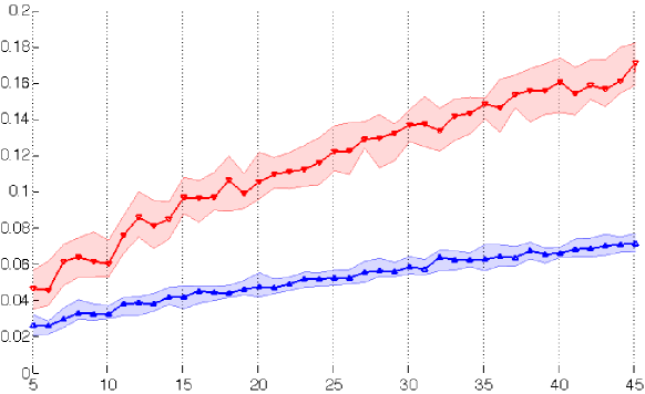
Figure 1: Variance comparison of the spectral and empirical least squares estimators. The upper curve (in red) present the performance (median value of the variance over 40 iterations) of the spectral method while the lower curve (in blue) the performance of the empirical least squares estimator. For each curve, we have plotted a shaded box plot representing the first and third quartiles.

The quadratic loss can be expressed as a variance term and a bias term as follows

$$\forall 1\leq k\leq K,\ \forall M\geq 0,\quad\|f^{\star}_{k}-\hat{f}_{k}\|_{2}^{2}=\|\hat{f}_{k}-f^{\star}_{M,k}\|_{2}^{2}+\|f^{\star}_{k}-f^{\star}_{M,k}\|_{2}^{2}$$

where $f^{\star}_{M,k}$ is the orthogonal projection of $f_{k}^{\star}$ on $\mathfrak{P}_{M}$ and $\hat{f}_{k}$ is any estimator such that $\hat{f}_{k}$ belongs to $\mathfrak{P}_{M}$. Note that the bias term $\|f^{\star}_{k}-f^{\star}_{M,k}\|_{2}$ does not depend on the estimator $\hat{f}_{k}$. Hence, the variance term

$$\mathrm{Variance}_{M}(\hat{f}):=\min_{\tau\in\mathfrak{S}_{K}}\max_{1\leq k\leq K}\|\hat{f}_{k}-f^{\star}_{M,\tau(k)}\|_{2}^{2}\,,$$

accounts for the performances of the estimator $\hat{f}_{k}$.

As depicted in Figure 1, we have compared, for each $M$, the variance terms obtained by the spectral method and the empirical least squares method over $40$ iterations on chains of length $N=5e4$. We have considered $K=2$ hidden states whose emission variables are distributed with respect to beta laws of parameters $(2,5)$ and $(4,2)$. This numerical experiment consolidates the idea that the least squares method significantly improves upon the spectral method. Indeed, even for small values of $M$, one may see in Figure 1 that the variance term is divided by a constant factor.

6.4 Histogram basis and trigonometric basis as approximation spaces

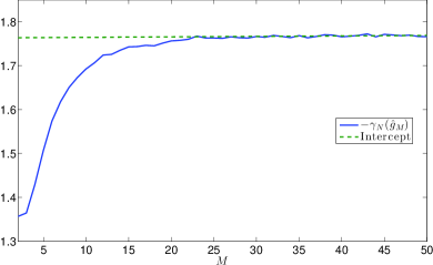
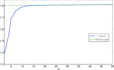
Figure 2: Slope heuristic to choose $M$: the experimenter may observe a linear stabilization of the empirical contrast $\gamma_{N}$ for estimating beta emission laws of parameters $(2,5)$ and $(4,2)$. We have $K=2$ hidden states and $N=5e4$ samples along a single chain. On the left panel we have used the trigonometric basis as approximation space, the stabilization occurs on the points $M=30$ to $M=50$ and the interpolation of the slope leads to $\hat{M}=23$. On the right panel we have considered the trigonometric basis, the stabilization occurs on the points $M=20$ to $M=50$ and it leads to $\hat{M}=21$.

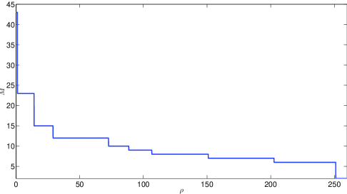
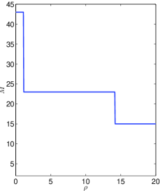
Figure 3: Slope heuristic to choose $M$: the experimenter observes the largest drop of the function $\rho\mapsto\hat{M}(\rho)$ at $1.1$ so that $\hat{\rho}=2.2$ and $\hat{M}=23$. We have $K=2$ hidden states and a single chain of length $N=5e4$. We have used the histogram basis as approximation space.

An illustrative example of our method can be given using the histogram basis (regular basis with $M$ bins) or the trigonometric basis. In the following experiments, we have $K=2$ hidden states and emission laws given by beta laws of parameters $(2,5)$ and $(4,2)$. Recall we observe a single chain of length $N=5e4$.

We begin with the computation of the minimum contrast function $M\mapsto\gamma(\hat{g}_{M})$, as depicted in Figure 2. Observe that the slope of this function unquestionably stabilizes at a critical value refer to as $\hat{\rho}/2$ in both the histogram and the trigonometric case. This leads to an adaptive choice of $\hat{M}=23$ for the histogram basis and $\hat{M}=21$ for the trigonometric basis, see Figures 2 and 3.

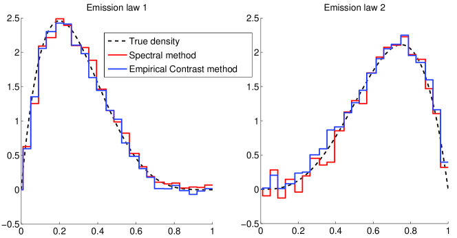
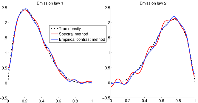
Figure 4: Estimators of the emissions densities (beta laws of parameters $(2,5)$ and $(4,2)$) from the observation of a single chain of length $N=5e4$. On the top panels, we have used the histogram basis ($\hat{M}=23$). On the bottom panels, we have considered the trigonometric basis ($\hat{M}=21$).

Furthermore, one can see on Figure 4 that our method also qualitatively improves upon the spectral method in both the histogram and the trigonometric case.

6.5 Three states

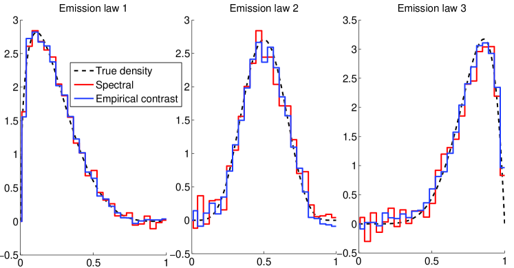
Figure 5: Estimation of three densities given by beta laws of parameters $(1.5,5)$, $(6,6)$ and $(7,2)$ from a single chain of length $N=5e4$. We have used the histogram basis and we have found $\hat{M}=25$ using the slope heuristic.

Our method can be performed for $K>2$ as illustrated in Figure 5. In this example $K=3$, the sample size is $N=5e4$ and the emission laws are three beta distributions with parameters $(1.5,5)$, $(6,6)$ and $(7,2)$. Note that the number of hidden states $K$ does not really impact on the complexity of the algorithm as we have seen in Section 6.2.

In this example, we were able to observe a linear stabilization of the minimum contrast function. The slope heuristic procedure led to an adaptive choice $\hat{M}=25$.

7 Discussion

We have proposed a penalized least squares method to estimate the emission densities of the hidden chain when the transition matrix of the hidden chain is full rank and the emission probability distributions are linearly independent. The algorithm may be initialized using spectral estimators. The obtained estimators are adaptive rate optimal up to a $\log$ factor, where adaptivity is upon the family of emission densities. The results hold under an assumption on the parameter that holds generically. We have proved that this assumption is always verified when there are two hidden states. We did not find a general argument to prove that the assumption always holds when $K>2$, and a natural question is to ask if, when the number of hidden states is $K>2$, this assumption is also always verified.
It is proved in Alexandrovich and Holzmann (2014) that identifiability holds as soon as $f_{1}^{\star},\ldots,f_{K}^{\star}$ are distinct densities. The identifiability is obtained in that case using the marginal distribution of dimension $2K+1$, that is the marginal distribution of $Y_{1},\ldots,Y_{2K+1}$. Thus, to get consistent estimators, one needs to use the joint distribution of $2K+1$ consecutive observations. Though linear independence is generically satisfied, one may wonder what happens when emission densities are not far to be linearly dependent. Simulations in Lehéricy (2015a) show that estimation becomes harder. In those practical situations where estimation becomes difficult, it is observed that the Gram matrix of $f_{1}^{\star},\ldots,f_{K}^{\star}$ has an eigenvalue close to $0$. On the theoretical side, the proof of Theorem 6 uses the linear independence of the emission densities by using that Gram matrices are positive. An interesting problem would be to investigate if it is possible to estimate the emission densities with the classical adaptive rate for density estimation when the emission densities are linearly dependent (though all distinct). It is possible using model selection to get the classical rate for the estimation of the density of $2K+1$ consecutive observations, but it does not seem obvious to see whether this rate can be transferred to the estimators of the emission densities. This is the subject of further work, see Lehéricy (2015b).
Another question arising from our work is whether it is possible to adapt to different smoothnesses of the emission densities.

8 Proofs

8.1 Proof of lemma 3

In Hsu et al. (2012) it is proved that when [H1], [H2], [H3] hold and when the rank of the matrix $\mathbf{O}_{M}:=(\langle\varphi_{m},f^{\star}_{k})_{1\leq m\leq M,1\leq k\leq K}$ is $K$, the knowledge of the tensor $\mathbf{M}_{M}$ given by $\mathbf{M}_{M}(a,b,c)=\mathbb{E}(\varphi_{a}(Y_{1})\varphi_{b}(Y_{2})\varphi_{c}(Y_{3}))$ for all $a,b,c$ in $\{1,\ldots,M\}$ allows to recover $\mathbf{O}_{M}$ and $\mathbf{Q}$ up to relabelling of the hidden states. Thus, when [H1], [H2], [H3] and [H4] hold, the knowledge of $g^{\mathbf{Q},\mathbf{f}^{\star}}$ is equivalent to the knowledge of the sequence $(\mathbf{M}_{M})_{M}$, which allows to recover $\mathbf{Q}$ and the sequence $(\mathbf{O}_{M})_{M}$, up to relabelling of the hidden states, which allows to recover $\mathbf{f}^{\star}=(f_{1}^{\star},\ldots,f_{K}^{\star})$ up to relabelling of the hidden states, thanks to (1). See also Gassiat et al. (2015).

8.2 Proof of Theorem 4

Throughout the proof $N$ is fixed, and we write $\gamma$ (instead of $\gamma_{N}$) for the contrast function.

8.2.1 Beginning of the proof: algebraic manipulations

Let us fix some $M$ and some permutation $\tau$. Using the definitions of $\hat{g}_{M}$ and $\hat{M}$, we can write

$$\gamma(\hat{g}_{\hat{M}})+{\rm pen}(N,\hat{M})\leq\gamma(\hat{g}_{M})+{\rm pen}(N,M)\leq\gamma(g^{\hat{\mathbf{Q}},\mathbf{f}^{\star}_{M,\tau^{-1}}})+{\rm pen}(N,M)\,,$$

where $\mathbf{f}^{\star}_{M,\tau^{-1}}=(f^{\star}_{M,\tau^{-1}(1)},\dots,f^{\star}_{M,\tau^{-1}(K)})$ (here we use that $\mathbf{f}^{\star}_{M,\tau^{-1}}\in\mathcal{F}^{K}$). But we can compute for all functions $t_{1},t_{2}$,

$$\gamma(t_{1})-\gamma(t_{2})=\lVert t_{1}-g^{\star}\lVert_{2}^{2}-\lVert t_{2}-g^{\star}\lVert_{2}^{2}-2\nu(t_{1}-t_{2})\,,$$

where $\nu$ is the centered empirical process

$$\nu(t)=\frac{1}{N}\sum_{s=1}^{N}t(Y_{1}^{(s)},Y_{2}^{(s)},Y_{3}^{(s)})-\int tg^{\star}\,.$$

This gives

$$\lVert\hat{g}_{\hat{M}}-g^{\star}\lVert_{2}^{2}\leq\lVert g^{\hat{\mathbf{Q}},\mathbf{f}^{\star}_{M,\tau^{-1}}}-g^{\star}\lVert_{2}^{2}+2\nu(\hat{g}_{\hat{M}}-g^{\hat{\mathbf{Q}},\mathbf{f}^{\star}_{M,\tau^{-1}}})+{\rm pen}(N,M)-{\rm pen}(N,\hat{M})$$ (4)

Now, we denote by $B_{M}=\lVert g^{\mathbf{Q}^{\star},\mathbf{f}^{\star}_{M}}-g^{\star}\lVert_{2}^{2}$ a bias term and we notice that $g^{\hat{\mathbf{Q}},\mathbf{f}^{\star}_{M,\tau^{-1}}}=g^{\mathbb{P}_{\tau}\hat{\mathbf{Q}}\mathbb{P}_{\tau}^{\top},\mathbf{f}^{\star}_{M}}$. Then

$$\lVert g^{\hat{\mathbf{Q}},\mathbf{f}^{\star}_{M,\tau^{-1}}}-g^{\star}\lVert_{2}^{2} \leq 2\lVert g^{\hat{\mathbf{Q}},\mathbf{f}^{\star}_{M,\tau^{-1}}}-g^{\mathbf{Q}^{\star},\mathbf{f}^{\star}_{M}}\lVert_{2}^{2}+2\lVert g^{\mathbf{Q}^{\star},\mathbf{f}^{\star}_{M}}-g^{\star}\lVert_{2}^{2}$$

$$\leq 2\lVert g^{\mathbb{P}_{\tau}\hat{\mathbf{Q}}\mathbb{P}_{\tau}^{\top},\mathbf{f}^{\star}_{M}}-g^{\mathbf{Q}^{\star},\mathbf{f}^{\star}_{M}}\lVert_{2}^{2}+2B_{M}.$$

But, using Schwarz inequality, $\lVert g^{\mathbf{Q}_{1},\mathbf{f}^{\star}_{M}}-g^{\mathbf{Q}_{2},\mathbf{f}^{\star}_{M}}\lVert_{2}^{2}$ can be bounded by

$$\sum_{m_{1},m_{2},m_{3}=1}^{M}\Big{|}\sum_{k_{1},k_{2},k_{3}=1}^{K}\left(\pi_{1}(k_{1})\mathbf{Q}_{1}(k_{1},k_{2})\mathbf{Q}_{1}(k_{2},k_{3})-\pi_{2}(k_{1})\mathbf{Q}_{2}(k_{1},k_{2})\mathbf{Q}_{2}(k_{2},k_{3})\right)$$

$$\quad\quad\quad\langle f^{\star}_{k_{1}},\varphi_{m_{1}}\rangle\langle f^{\star}_{k_{2}},\varphi_{m_{2}}\rangle\langle f^{\star}_{k_{3}},\varphi_{m_{3}}\rangle\Big{|}^{2}$$

$$\leq\left(\sum_{k_{1},k_{2},k_{3}=1}^{K}\left(\pi_{1}(k_{1})\mathbf{Q}_{1}(k_{1},k_{2})\mathbf{Q}_{1}(k_{2},k_{3})-\pi_{2}(k_{1})\mathbf{Q}_{2}(k_{1},k_{2})\mathbf{Q}_{2}(k_{2},k_{3})\right)^{2}\right)$$

$$\sum_{m_{1},m_{2},m_{3}=1}^{M}\,\sum_{k_{1},k_{2},k_{3}=1}^{K}\Big{|}\langle f^{\star}_{k_{1}},\varphi_{m_{1}}\rangle\langle f^{\star}_{k_{2}},\varphi_{m_{2}}\rangle\langle f^{\star}_{k_{3}},\varphi_{m_{3}}\rangle\Big{|}^{2}$$

$$\leq 3K^{3}C_{\mathcal{F},2}^{6}\left(\lVert\pi_{1}-\pi_{2}\lVert_{2}^{2}+2\lVert\mathbf{Q}_{1}-\mathbf{Q}_{2}\lVert_{F}^{2}\right)$$ (5)

so that

$$\lVert g^{\hat{\mathbf{Q}},\mathbf{f}^{\star}_{M,\tau^{-1}}}-g^{\star}\lVert_{2}^{2} \leq 6K^{3}C_{\mathcal{F},2}^{6}\left(\lVert\mathbb{P}_{\tau}\hat{\pi}-\pi^{\star}\lVert_{2}^{2}+2\lVert\mathbb{P}_{\tau}\hat{\mathbf{Q}}\mathbb{P}_{\tau}^{\top}-\mathbf{Q}^{\star}\lVert_{F}^{2}\right)+2B_{M}.$$

Next we set $S_{M}=\cup_{\mathbf{Q}}\mathcal{S}({\mathbf{Q}},{M})$ and

$$Z_{M}=\sup_{t\in S_{M}}\left[\frac{|\nu(t-g^{\star})|}{\lVert t-g^{\star}\lVert_{2}^{2}+x_{M}^{2}}\right]$$

for $x_{M}$ to be determined later. Then

$$\nu(\hat{g}_{\hat{M}}-g^{\hat{\mathbf{Q}},\mathbf{f}^{\star}_{M,\tau^{-1}}}) = \nu(\hat{g}_{\hat{M}}-g^{\star})+\nu(g^{\star}-g^{\hat{\mathbf{Q}},\mathbf{f}^{\star}_{M,\tau^{-1}}})$$

$$\leq Z_{\hat{M}}(\lVert\hat{g}_{\hat{M}}-g^{\star}\lVert_{2}^{2}+x_{\hat{M}}^{2})+Z_{M}(\lVert g^{\hat{\mathbf{Q}},\mathbf{f}^{\star}_{M,\tau^{-1}}}-g^{\star}\lVert_{2}^{2}+x_{M}^{2}).$$

Denoting by $R_{\hat{M}}=\lVert\hat{g}_{\hat{M}}-g^{\star}\lVert_{2}^{2}$ the squared risk, (4) becomes

$$R_{\hat{M}} \leq 6K^{3}C_{\mathcal{F},2}^{6}\left(\lVert\mathbb{P}_{\tau}\hat{\pi}-\pi^{\star}\lVert_{2}^{2}+2\lVert\mathbb{P}_{\tau}\hat{\mathbf{Q}}\mathbb{P}_{\tau}^{\top}-\mathbf{Q}^{\star}\lVert_{F}^{2}\right)+2B_{M}+2Z_{\hat{M}}(R_{\hat{M}}+x_{\hat{M}}^{2})$$

$$+2Z_{M}\left(6K^{3}C_{\mathcal{F},2}^{6}\left(\lVert\mathbb{P}_{\tau}\hat{\pi}-\pi^{\star}\lVert_{2}^{2}+2\lVert\mathbb{P}_{\tau}\hat{\mathbf{Q}}\mathbb{P}_{\tau}^{\top}-\mathbf{Q}^{\star}\lVert_{F}^{2}\right)+2B_{M}+x_{M}^{2}\right)$$

$$+2{\rm pen}(N,M)-{\rm pen}(N,\hat{M})-{\rm pen}(N,M)\,,$$

$$R_{\hat{M}}(1-2Z_{\hat{M}}) \leq (2+4Z_{M})B_{M}+2{\rm pen}(N,M)$$

$$+(1+2Z_{M})6K^{3}C_{\mathcal{F},2}^{6}\left(\lVert\mathbb{P}_{\tau}\hat{\pi}-\pi^{\star}\lVert_{2}^{2}+2\lVert\mathbb{P}_{\tau}\hat{\mathbf{Q}}\mathbb{P}_{\tau}^{\top}-\mathbf{Q}^{\star}\lVert_{F}^{2}\right)$$

$$+2\sup_{M^{\prime}}(2Z_{M^{\prime}}x_{M^{\prime}}^{2}-{\rm pen}(N,M^{\prime}))\,.$$

To conclude it is then sufficient to establish that, with probability larger than $1-(e-1)^{-1}e^{-x}$, it holds

$$\sup_{M^{\prime}}Z_{M^{\prime}}\leq\frac{1}{4}\quad\text{ and }\quad\sup_{M^{\prime}}(2Z_{M^{\prime}}x_{M^{\prime}}^{2}-{\rm pen}(N,M^{\prime}))\leq A\frac{x}{N}\,,$$

with $A$ a constant depending only on $\mathbf{Q}^{\star}$ and $\mathbf{f}^{\star}$ and not on $N,M,x$. Thus we will have, for any $M$, with probability larger than $1-(e-1)^{-1}e^{-x}$,

$$\frac{1}{2}R_{\hat{M}} \leq 3B_{M}+2{\rm pen}(N,M)+2A\frac{x}{N}$$

$$+9C_{\mathcal{F},2}^{6}\left(\lVert\mathbb{P}_{\tau}\hat{\pi}-\pi^{\star}\lVert_{2}^{2}+2\lVert\mathbb{P}_{\tau}\hat{\mathbf{Q}}\mathbb{P}_{\tau}^{\top}-\mathbf{Q}^{\star}\lVert_{F}^{2}\right)$$

which is the announced result.

The heart of the proof is then the study of $Z_{M}$. We introduce $u_{M}$ a projection of $g^{\star}$ on $S_{M}$ and we split $Z_{M}$ into two terms: $Z_{M}\leq 4Z_{M,1}+Z_{M,2}$ with

$$\begin{cases}\displaystyle Z_{M,1}=\sup_{t\in S_{M}}\left[\frac{|\nu(t-u_{M})|}{\lVert t-u_{M}\lVert_{2}^{2}+4x_{M}^{2}}\right]\\ \displaystyle Z_{M,2}=\frac{|\nu(u_{M}-g^{\star})|}{\lVert u_{M}-g^{\star}\lVert_{2}^{2}+x_{M}^{2}}\end{cases}$$

Indeed $u_{M}$ verifies: for all $t\in S_{M}$,

$$\lVert u_{M}-g^{\star}\lVert_{2}\leq\lVert t-g^{\star}\lVert_{2}\quad\mathrm{and}\quad\lVert u_{M}-t\lVert_{2}\leq 2\lVert t-g^{\star}\lVert_{2}\,.$$

8.2.2 Deviation inequality for $Z_{M,2}$

Bernstein’s inequality (24) for HMMs (see Appendix A) gives, with probability larger than $1-e^{-z}$:

$$|\nu(u_{M}-g^{\star})|\leq 2\sqrt{2c^{\star}\lVert u_{M}-g^{\star}\lVert_{2}^{2}\lVert g^{\star}\lVert_{\infty}\frac{z}{N}}+2\sqrt{2}c^{\star}\lVert u_{M}-g^{\star}\lVert_{\infty}\frac{z}{N}\,.$$

Then, using $a^{2}+b^{2}\geq 2ab$, with probability larger than $1-e^{-z}$:

$$\frac{|\nu(u_{M}-g^{\star})|}{\lVert u_{M}-g^{\star}\lVert_{2}^{2}+x_{M}^{2}} \leq 2\sqrt{2c^{\star}\lVert g^{\star}\lVert_{\infty}}\frac{1}{2x_{M}}\sqrt{\frac{z}{N}}+2\sqrt{2}c^{\star}\frac{\lVert u_{M}\lVert_{\infty}+\lVert g^{\star}\lVert_{\infty}}{x_{M}^{2}}\frac{z}{N}\,.$$

But any function $t$ in $S_{M}$ can be written

$$t=\sum_{k_{1},k_{2},k_{3}=1}^{K}\pi(k_{1})\mathbf{Q}(k_{1},k_{2})\mathbf{Q}(k_{2},k_{3})f_{k_{1}}\otimes f_{k_{2}}\otimes f_{k_{3}}\,,$$

with $f_{k}\in\mathcal{F}$ for $k=1,\dots,K$, so that $\sup_{t\in S_{M}}\lVert t\lVert_{\infty}\leq C_{\mathcal{F},\infty}^{3}$. Then, with probability larger than $1-e^{-z_{M}-z}$

$$Z_{M,2}\leq\sqrt{2c^{\star}\lVert g^{\star}\lVert_{\infty}}\sqrt{\frac{z_{M}+z}{x_{M}^{2}N}}+4\sqrt{2}c^{\star}C_{\mathcal{F},\infty}^{3}\frac{z_{M}+z}{x_{M}^{2}N}\,.$$ (6)

8.2.3 Deviation inequality for $Z_{M,1}$

We shall first study the term $\sup_{t\in B_{\sigma}}|\nu(t-u_{M})|$ where

$$B_{\sigma}=\{t\in S_{M},\lVert t-u_{M}\lVert_{2}\leq\sigma\}.$$

Remark that, for all $t\in\mathcal{S}({\mathbf{Q}},{M})$,

$$\lVert t\lVert_{2}^{2}\leq\sum_{k_{1},k_{2},k_{3}=1}^{K}\pi^{2}(k_{1})\mathbf{Q}^{2}(k_{1},k_{2})\mathbf{Q}^{2}(k_{2},k_{3})\sum_{k_{1},k_{2},k_{3}=1}^{K}C_{\mathcal{F},2}^{2}C_{\mathcal{F},2}^{2}C_{\mathcal{F},2}^{2}\leq K^{3}C_{\mathcal{F},2}^{6}.$$

Then, if $t\in B_{\sigma}$, $\lVert t-u_{M}\lVert_{2}\leq\sigma\wedge 2K^{3/2}C_{\mathcal{F},2}^{3}$. Notice also that for all $t\in S_{M}$, $\lVert t-u_{M}\lVert_{\infty}\leq 2C_{\mathcal{F},\infty}^{3}$. Now Proposition 13 in Appendix A (applied to a countable dense set in $B_{\sigma}$) gives that for any measurable set $A$ such that $\mathbb{P}(A)>0$,

$$\mathbb{E}^{A}(\sup_{t\in B_{\sigma}}|\nu(t-u_{M})|)\leq C^{\star}\left[\frac{E}{N}+\sigma\sqrt{\frac{1}{N}\log\left(\frac{1}{\mathbb{P}(A)}\right)}+\frac{2C_{\mathcal{F},\infty}^{3}}{N}\log\left(\frac{1}{\mathbb{P}(A)}\right)\right],$$

and

$$E=\sqrt{N}\int_{0}^{\sigma}\sqrt{H(u)\wedge N}du+(2C_{\mathcal{F},\infty}^{3}+2K^{3/2}C_{\mathcal{F},2}^{3})H(\sigma)\,.$$

Here, for any integrable random variable $Z$, $E^{A}[Z]$ denotes $E[Z\mathds{1}_{A}]/\mathbb{P}(A)$.

We shall compute $E$ later and find $\sigma_{M}$ and $\varphi$ such that

$$\forall\sigma\geq\sigma_{M}\qquad E\leq(1+2C_{\mathcal{F},\infty}^{3}+2K^{3/2}C_{\mathcal{F},2}^{3})\varphi(\sigma)\sqrt{N}.$$ (7)

(see Section 8.2.4). We then use Lemma 4.23 in Massart (2007) to write (for $x_{M}\geq\sigma_{M}$)

$$\mathbb{E}^{A}\left(\sup_{t\in S_{M}}\left[\frac{|\nu(t-u_{M})|}{\lVert t-u_{M}\lVert_{2}^{2}+4x_{M}^{2}}\right]\right)\leq\frac{C^{\star}}{x_{M}^{2}}\left[C\frac{\varphi(2x_{M})}{\sqrt{N}}+2x_{M}\sqrt{\frac{1}{N}\log\left(\frac{1}{\mathbb{P}(A)}\right)}+\frac{2C_{\mathcal{F},\infty}^{3}}{N}\log\left(\frac{1}{\mathbb{P}(A)}\right)\right]$$

Finally, Lemma 2.4 in Massart (2007) ensures that, with probability $1-e^{-z_{M}-z}$:

$$Z_{M,1}=\sup_{t\in S_{M}}\left[\frac{|\nu(t-u_{M})|}{\lVert t-u_{M}\lVert_{2}^{2}+4x_{M}^{2}}\right]\leq C^{\star}\left[C\frac{\varphi(2x_{M})}{x_{M}^{2}\sqrt{N}}+2\sqrt{\frac{z_{M}+z}{x_{M}^{2}N}}+2C_{\mathcal{F},\infty}^{3}\frac{z_{M}+z}{x_{M}^{2}N}\right].$$ (8)

8.2.4 Computation of the entropy and function $\varphi$

The definition of $H$ given in Proposition 13 shows that $H(\delta)$ is bounded by the classical bracketing entropy for $\mathbf{L}^{2}$ distance at point $\delta/C_{\mathcal{F},\infty}^{3}$ (where $C_{\mathcal{F},\infty}^{3}$ bounds the sup norm of $g^{\star}$): $H(\delta)\leq H(\delta/C_{\mathcal{F},\infty}^{3},S_{M},\mathbf{L}^{2})$. We denote by $N(u,S,\mathbf{L}^{2})=e^{H(u,S,\mathbf{L}^{2})}$ the minimal number of brackets of radius $u$ to cover $S$. Recall that when $t_{1}$ and $t_{2}$ are real valued functions, the bracket $[t_{1},t_{2}]$ is the set of real valued functions $t$ such that $t_{1}(\cdot)\leq t(\cdot)\leq t_{2}(\cdot)$, and the radius of the bracket is $\|t_{2}-t_{1}\|_{2}$. Now, observe that $S_{M}=\cup_{\mathbf{Q}}\mathcal{S}({\mathbf{Q}},{M})$ is a set of mixtures of parametric functions. Denoting $\mathbf{k}=(k_{1},k_{2},k_{3})$, $S_{M}$ is included in

$$\left\{\sum_{\mathbf{k}\in\{1,\dots,K\}^{3}}\mu(\mathbf{k})f_{k_{1}}\otimes f_{k_{2}}\otimes f_{k_{3}},\ \mu\geq 0,\ \sum_{\mathbf{k}\in\{1,\dots,K\}^{3}}\mu(\mathbf{k})=1,\right.\\ \left.f_{k_{i}}\in{\mathcal{F}}\cap{\rm Span}(\varphi_{1},\dots,\varphi_{M}),\;i=1,2,3\right\}\,.$$

Set

$$\mathcal{A}=\{f_{1}\otimes f_{2}\otimes f_{3},f_{i}\in{\mathcal{F}}\cap{\rm Span}(\varphi_{1},\dots,\varphi_{M}),\;i=1,2,3\}.$$

Then following the proof in Appendix A of Bontemps and Toussile (2013), we can prove

$$N(\varepsilon,S_{M},\mathbf{L}^{2})\leq\left(\frac{C_{1}}{\varepsilon}\right)^{K^{3}-1}\left[N\left(\frac{\varepsilon}{3},\mathcal{A},\mathbf{L}^{2}\right)\right]^{K^{3}}\,.$$ (9)

where $C_{1}$ depends on $K$ and $C_{\mathcal{F},2}$. Denote $\mathcal{B}={\mathcal{F}}\cap{\rm Span}(\varphi_{1},\dots,\varphi_{M})$. Let $a=(a_{m})_{1\leq m\leq M}\in\mathbb{R}^{M}$ and $b=(b_{m})_{1\leq m\leq M}\in\mathbb{R}^{M}$ such that $a_{m}<b_{m}$, $m=1,\ldots,M$. For each $m=1,\ldots,M$ and $y\in\mathcal{Y}$, let

$$u_{m}(y) =\begin{cases}a_{m}\qquad\text{if }\varphi_{m}(y)\geq 0\\ b_{m}\qquad\text{otherwise}\end{cases}$$

$$v_{m}(y) =a_{m}+b_{m}-u_{m}(y).$$

Then, if $(c_{m})_{1\leq m\leq M}\in\mathbb{R}^{M}$ is such that for all $m=1,\ldots,M$, $a_{m}\leq c_{m}\leq b_{m}$, then

$$U_{a,b}^{1}(y):=\sum_{m=1}^{M}u_{m}(y)\varphi_{m}(y)\leq\sum_{m=1}^{M}c_{m}\varphi_{m}(y)\leq\sum_{m=1}^{M}v_{m}(y)\varphi_{m}(y)=U^{2}_{a,b}(y).$$

Moreover,

$$\|U^{2}_{a,b}-U^{1}_{a,b}\|_{2}^{2} =\|\sum_{m=1}^{M}|b_{m}-a_{m}|.|\varphi_{m}|\|_{2}^{2}$$

$$\leq M\|b-a\|_{2}^{2}$$

using Cauchy-Schwarz inequality. Thus, one may cover $\mathcal{B}$ with brackets of form $[U^{1}_{a,b},U^{2}_{a,b}]$. Also, for $i=1,2$,

$$\|U^{i}_{a,b}\|_{2}^{2} \leq\|\sum_{m_{i}=1}^{M}|b_{m}+a_{m}|.|\varphi_{m}|\|_{2}^{2}$$

$$\leq 2M(\|a\|_{2}^{2}+\|b\|_{2}^{2}).$$

If now for some $a^{i}$, $b^{i}$ in $\mathbb{R}^{M}$, $f_{i}\in[U^{1}_{a^{i},b^{i}},U^{2}_{a^{i},b^{i}}]$, $i=1,2,3$, then

$$f_{1}\otimes f_{2}\otimes f_{3}\in\left[V,W\right]$$

with

$$V=\min\{U^{i_{1}}_{a^{1},b^{1}}U^{i_{2}}_{a^{2},b^{2}}U^{i_{3}}_{a^{3},b^{3}},\;i_{1},i_{2},i_{3}\in\{1,2\}\}$$

and

$$W=\max\{U^{i_{1}}_{a^{1},b^{1}}U^{i_{2}}_{a^{2},b^{2}}U^{i_{3}}_{a^{3},b^{3}},\;i_{1},i_{2},i_{3}\in\{1,2\}\},$$

pointwise. Moreover, one can see that

$$\left|W-V\right| \leq \left|U^{2}_{a^{1},b^{1}}-U^{1}_{a^{1},b^{1}}\right|\max_{j_{1},j_{2}\in\{1,2\}}\left|U^{j_{1}}_{a^{2},b^{2}}\right|.\left|U^{j_{2}}_{a^{3},b^{3}}\right|$$

$$+\left|U^{2}_{a^{2},b^{2}}-U^{1}_{a^{2},b^{2}}\right|\max_{j_{1},j_{2}\in\{1,2\}}\left|U^{j_{1}}_{a^{1},b^{1}}\right|.\left|U^{j_{2}}_{a^{3},b^{3}}\right|$$

$$+\left|U^{2}_{a^{3},b^{3}}-U^{1}_{a^{3},b^{3}}\right|\max_{j_{1},j_{2}\in\{1,2\}}\left|U^{j_{1}}_{a^{1},b^{1}}\right|.\left|U^{j_{2}}_{a^{2},b^{2}}\right|$$

$$\leq \sum_{i=1}^{3}\left|U^{2}_{a^{i},b^{i}}-U^{1}_{a^{i},b^{i}}\right|\prod_{j\neq i}\left(\left|U^{1}_{a^{j},b^{j}}\right|+\left|U^{2}_{a^{j},b^{j}}\right|\right)$$

so that

$$\left\|W-V\right\|_{2}^{2} \leq 12\sum_{i=1}^{3}\left\|U^{2}_{a^{i},b^{i}}-U^{1}_{a^{i},b^{i}}\right\|_{2}^{2}\prod_{j\neq i}\left(\left\|U^{1}_{a^{j},b^{j}}\right\|_{2}^{2}+\left\|U^{2}_{a^{j},b^{j}}\right\|_{2}^{2}\right)$$

$$\leq 48M^{3}\sum_{i=1}^{3}\|b^{i}-a^{i}\|_{2}^{2}\prod_{j\neq i}\left(\|a^{j}\|_{2}^{2}+\|b^{j}\|_{2}^{2}\right)$$

$$\leq 192M^{3}C_{\mathcal{F},2}^{4}\sum_{i=1}^{3}\|b^{i}-a^{i}\|_{2}^{2}.$$

Thus one may cover $\mathcal{A}$ by covering the ball of radius $C_{\mathcal{F},2}$ in $\mathbb{R}^{M}$ with hypercubes $[a,b]$, for which $\|a\|_{2}$, $\|b\|_{2}$ are less than $C_{\mathcal{F},2}$. To get a bracket with radius $u$, it is enough that $\|b^{i}-a^{i}\|_{2}^{2}\leq u^{2}/(576M^{3}C_{\mathcal{F},2}^{4})$, $i=1,2,3$. We finally obtain that

$$N\left(u,\mathcal{A},\mathbf{L}^{2}\right)\leq\left(\frac{48\sqrt{3}M^{3/2}C_{\mathcal{F},2}^{3}}{u}\right)^{3M}.$$ (10)

We deduce from (9) and (10) that

$$N(u,S_{M},\mathbf{L}^{2})\leq\left(\frac{C_{1}}{u}\right)^{K^{3}-1}\left(\frac{48\sqrt{3}M^{3/2}C_{\mathcal{F},2}^{3}}{u}\right)^{3MK^{3}}\,,$$

and then

$$H(u,S_{M},\mathbf{L}^{2})\leq(K^{3}-1)\log(\frac{C_{1}}{u})+3MK^{3}\log\left(\frac{C_{2}M^{3/2}}{u}\right)\,,$$

with $C_{2}$ depending on $K$ and $C_{\mathcal{F},2}$. To conclude we use that $\int_{0}^{\sigma}\sqrt{\log\left(\frac{1}{x}\right)}dx\leq\sigma(\sqrt{\pi}+\sqrt{\log\left(\frac{1}{\sigma}\right)})$, see Baudry et al. (2012). Finally we can write for $\sigma\leq M^{3/2}$:

$$\int_{0}^{\sigma}\sqrt{H(u)}du\leq C_{3}\sqrt{M}\sigma\left(1+\sqrt{\log\left(\frac{M^{3/2}}{\sigma}\right)}\right),$$

where $C_{3}$ depends on $K$, $C_{\mathcal{F},2}$ and $C_{\mathcal{F},\infty}$. Set

$$\varphi(x)=C_{3}\sqrt{M}x\left(1+\sqrt{\log\left(\frac{M^{3/2}}{x}\right)}\right)$$

The function $\varphi$ is increasing on $]0,M^{3/2}]$, and $\varphi(x)/x$ is decreasing. Moreover $\varphi(\sigma)\geq\int_{0}^{\sigma}\sqrt{H(u)}du$ and $\varphi^{2}(\sigma)\geq\sigma^{2}H(\sigma)$.

8.2.5 End of the proof, choice of parameters

As soon as $N\geq C_{3}^{2}/M^{2}:=N_{0}$, we may define $\sigma_{M}$ as the solution of equation $\varphi(x)=\sqrt{N}x^{2}$. Then, for all $\sigma\geq\sigma_{M}$,

$$H(\sigma)\leq\frac{\varphi(\sigma)^{2}}{\sigma^{2}}\leq\frac{\varphi(\sigma)}{\sigma}\sigma\sqrt{N}.$$

This yields, for all $\sigma\geq\sigma_{M},$

$$E\leq(1+2C_{\mathcal{F},\infty}^{3}+2K^{3/2}C_{\mathcal{F},2}^{3})\varphi(\sigma)\sqrt{N},$$

which was required in (7).

Moreover $\frac{\varphi(2x_{M})}{x_{M}\sqrt{N}}\leq 2\sigma_{M}$ as soon as $x_{M}\geq\sigma_{M}$. Combining (8) and (6), we obtain, with probability $1-e^{-z_{M}-z}$:

$$Z_{M}\leq C^{\star\star}\left[\frac{\sigma_{M}}{x_{M}}+\sqrt{\frac{z_{M}+z}{x_{M}^{2}N}}+\frac{z_{M}+z}{x_{M}^{2}N}\right]\,,$$

where $C^{\star\star}$ depends on $K$, $C_{\mathcal{F},2}$, $C_{\mathcal{F},\infty}$, $\mathbf{Q}^{\star}$. Now let us choose $x_{M}=\theta^{-1}\sqrt{\sigma_{M}^{2}+\frac{z_{M}+z}{N}}$ with $\theta$ such that $2\theta+\theta^{2}\leq(C^{\star\star})^{-1}/4$. This choice entails: $x_{M}\geq\theta^{-1}\sigma_{M}$ and $x_{M}^{2}\geq\theta^{-2}\frac{z_{M}+z}{N}.$ Then with probability $1-e^{-z_{M}-z}$:

$$Z_{M}\leq C^{\star\star}(\theta+\theta+\theta^{2}).$$

We now choose $z_{M}=M$ which implies $\sum_{M\geq 1}e^{-z_{M}}=(e-1)^{-1}$. Then, with probability $1-(e-1)^{-1}e^{-z}$,

$$\forall M\qquad Z_{M}\leq C^{\star\star}(2\theta+\theta^{2})\leq\frac{1}{4}\,,$$

and for all $M$,

$$Z_{M}x_{M}^{2} \leq C^{\star\star}\left[{\sigma_{M}}{x_{M}}+x_{M}\sqrt{\frac{z_{M}+z}{N}}+\frac{z_{M}+z}{N}\right]$$

$$\leq C^{\star\star}\theta^{-1}\left(\sigma_{M}+\sqrt{\frac{z_{M}+z}{N}}\right)^{2}+C^{\star\star}\frac{z_{M}+z}{N}\,.$$

Then, with probability $1-(e-1)^{-1}e^{-z}$, for all $M$,

$$Z_{M}x_{M}^{2}-C^{\star\star}\left(2\theta^{-1}\sigma_{M}^{2}+(2\theta^{-1}+1)\frac{M}{N}\right)\leq C^{\star\star}(2\theta^{-1}+1)\frac{z}{N}\,.$$

Then the result is proved as soon as

$${\rm pen}(N,M)\geq 2C^{\star\star}\left(2\theta^{-1}\sigma_{M}^{2}+(2\theta^{-1}+1)\frac{M}{N}\right).$$ (11)

It remains to get an upper bound for $\sigma_{M}$. Recall that $\sigma_{M}$ is defined as the solution of equation $C_{3}\sqrt{M}x(1+\sqrt{\log\left(\frac{M^{3}}{x}\right)})=\sqrt{N}x^{2}$. Then we obtain that for some $C_{4}$

$$\sigma_{M}\leq C_{4}\sqrt{\frac{M}{N}}(1+\sqrt{\log(N)})\,,$$

and (11) holds as soon as

$${\rm pen}(N,M)\geq\rho^{\star}\frac{M\log(N)}{N}$$

for some constant $\rho^{\star}$ depending on $C_{\mathcal{F},2}$ and $C_{\mathcal{F},\infty}$ (Scenario A) or on $\mathbf{Q}^{\star}$, $C_{\mathcal{F},2}$ and $C_{\mathcal{F},\infty}$ (Scenario B).

8.3 Proof of Theorem 6

For any $\mathbf{h}\in{\mathcal{K}}^{K}$ and $\mathbf{Q}\in{\mathcal{V}}$, denote $N(\mathbf{Q},\mathbf{h})=\lVert g^{\mathbf{Q},\mathbf{f}^{\star}+\mathbf{h}}-g^{\mathbf{Q},\mathbf{f}^{\star}}\lVert_{2}^{2}$. What we want to prove is that

$$c:=c({\mathcal{K}},{\mathcal{V}},\mathfrak{F}^{\star})^{2}:=\inf_{\mathbf{Q}\in{\mathcal{V}},\mathbf{h}\in{\mathcal{K}}^{K},\lVert{\mathbf{h}}\lVert_{2}\neq 0}\frac{N({\mathbf{Q}},{\mathbf{h}})}{\lVert{\mathbf{h}}\lVert_{{2}}^{2}}>0.$$

One can compute:

$$N(\mathbf{Q},\mathbf{h})=\sum_{k_{1},k_{2},k_{3},k^{\prime}_{1},k^{\prime}_{2},k^{\prime}_{3}=1}^{K}\pi(k_{1})\mathbf{Q}(k_{1},k_{2})\mathbf{Q}(k_{2},k_{3})\pi(k^{\prime}_{1})\mathbf{Q}(k^{\prime}_{1},k^{\prime}_{2})\mathbf{Q}(k^{\prime}_{2},k^{\prime}_{3})\\ \left(\prod_{i=1}^{3}\langle f^{\star}_{k_{i}}+h_{k_{i}},f^{\star}_{k^{\prime}_{i}}+h_{k^{\prime}_{i}}\rangle+\prod_{i=1}^{3}\langle f^{\star}_{k_{i}},f^{\star}_{k^{\prime}_{i}}\rangle-\prod_{i=1}^{3}\langle f^{\star}_{k_{i}}+h_{k_{i}},f^{\star}_{k^{\prime}_{i}}\rangle-\prod_{i=1}^{3}\langle f^{\star}_{k_{i}},f^{\star}_{k^{\prime}_{i}}+h_{k^{\prime}_{i}}\rangle\right).$$

Let ${\mathbf{u}}=(u_{1},\ldots,u_{K})$ be such that $u_{i}$, $i=1,\ldots,K$, is the orthogonal projection of $h_{i}$ on the subspace of $\mathbf{L}^{2}(\mathcal{Y},\mathcal{L}^{D})$ spanned by $f_{1}^{\star}\ldots,f_{K}^{\star}$. Then

$$N(\mathbf{Q},\mathbf{h})=N(\mathbf{Q},\mathbf{u})+M(\mathbf{Q},\mathbf{u},\mathbf{h}-\mathbf{u})$$ (12)

where, for any $\mathbf{a}=(a_{1},\ldots,a_{K})\in\mathbf{L}^{2}(\mathcal{Y},\mathcal{L}^{D})^{K}$,

$$M(\mathbf{Q},\mathbf{u},\mathbf{a})=\sum_{k_{1},k_{2},k_{3},k^{\prime}_{1},k^{\prime}_{2},k^{\prime}_{3}=1}^{K}\pi(k_{1})\mathbf{Q}(k_{1},k_{2})\mathbf{Q}(k_{2},k_{3})\pi(k^{\prime}_{1})\mathbf{Q}(k^{\prime}_{1},k^{\prime}_{2})\mathbf{Q}(k^{\prime}_{2},k^{\prime}_{3})\\ \left(\prod_{i=1}^{3}\langle a_{k_{i}},a_{k^{\prime}_{i}}\rangle+\sum_{i=1}^{3}\langle a_{k_{i}},a_{k^{\prime}_{i}}\rangle\prod_{j\neq i}\langle f^{\star}_{k_{j}}+u_{k_{j}},f^{\star}_{k^{\prime}_{j}}+u_{k^{\prime}_{j}}\rangle+\sum_{i=1}^{3}\langle f^{\star}_{k_{i}}+u_{k_{i}},f^{\star}_{k^{\prime}_{i}}+u_{k^{\prime}_{i}}\rangle\prod_{j\neq i}\langle a_{k_{j}},a_{k^{\prime}_{j}}\rangle\right).$$

Let $A=\mathfrak{Diag}[{\pi}]$ with $\pi$ the stationary distribution of $\mathbf{Q}$. Then $M(\mathbf{Q},\mathbf{u},\mathbf{a})$ may be rewritten as:

$$M(\mathbf{Q},\mathbf{u},\mathbf{a}) =\sum_{i,j=1}^{K} \langle(\mathbf{Q}^{T}A\mathbf{a})_{i},(\mathbf{Q}^{T}A\mathbf{a})_{j}\rangle\langle{a}_{i},{a}_{j}\rangle\langle(\mathbf{Q}\mathbf{a})_{i},(\mathbf{Q}\mathbf{a})_{j}\rangle$$

$$+\langle(\mathbf{Q}^{T}A\mathbf{a})_{i},(\mathbf{Q}^{T}A\mathbf{a})_{j}\rangle\langle(\mathbf{f}^{\star}+\mathbf{u}_{i}),(\mathbf{f}^{\star}+\mathbf{u})_{j}\rangle\langle(\mathbf{Q}(\mathbf{f}^{\star}+\mathbf{u}))_{i},(\mathbf{Q}(\mathbf{f}^{\star}+\mathbf{u}))_{j}\rangle$$

$$+\langle(\mathbf{Q}^{T}A(\mathbf{f}^{\star}+\mathbf{u}))_{i},(\mathbf{Q}^{T}A(\mathbf{f}^{\star}+\mathbf{u}))_{j}\rangle\langle{a}_{i},{a}_{j}\rangle\langle(\mathbf{Q}(\mathbf{f}^{\star}+\mathbf{u}))_{i},(\mathbf{Q}(\mathbf{f}^{\star}+\mathbf{u}))_{j}\rangle$$

$$+\langle(\mathbf{Q}^{T}A(\mathbf{f}^{\star}+\mathbf{u}))_{i},(\mathbf{Q}^{T}A(\mathbf{f}^{\star}+\mathbf{u}))_{j}\rangle\langle(\mathbf{f}^{\star}+\mathbf{u})_{i},(\mathbf{f}^{\star}+\mathbf{u})_{j}\rangle\langle(\mathbf{Q}\mathbf{a})_{i},(\mathbf{Q}\mathbf{a})_{j}\rangle$$

$$+\langle(\mathbf{Q}^{T}A(\mathbf{f}^{\star}+\mathbf{u}))_{i},(\mathbf{Q}^{T}A(\mathbf{f}^{\star}+\mathbf{u}))_{j}\rangle\langle{a}_{i},{a}_{j}\rangle\langle(\mathbf{Q}\mathbf{a})_{i},(\mathbf{Q}\mathbf{a})_{j}\rangle$$

$$+\langle(\mathbf{Q}^{T}A\mathbf{a})_{i},(\mathbf{Q}^{T}A\mathbf{a})_{j}\rangle\langle(\mathbf{f}^{\star}+\mathbf{u})_{i},(\mathbf{f}^{\star}+\mathbf{u})_{j}\rangle\langle(\mathbf{Q}\mathbf{a})_{i},(\mathbf{Q}\mathbf{a})_{j}\rangle$$

$$+\langle(\mathbf{Q}^{T}A\mathbf{a})_{i},(\mathbf{Q}^{T}A\mathbf{a})_{j}\rangle\langle{a}_{i},{a}_{j}\rangle\langle(\mathbf{Q}(\mathbf{f}^{\star}+\mathbf{u}))_{i},(\mathbf{Q}(\mathbf{f}^{\star}+\mathbf{u}))_{j}\rangle.$$

All terms in this sum are non negative. Let us prove it for the first one, the argument for the others is similar. Define $V$ the $K\times K$ matrix given by

$$V_{i,j}=\langle(\mathbf{Q}^{T}A\mathbf{a})_{i},(\mathbf{Q}^{T}A\mathbf{a})_{j}\rangle\langle(\mathbf{Q}\mathbf{a})_{i},(\mathbf{Q}\mathbf{a})_{j}\rangle,\quad i,j=1,\ldots,K.$$

$V$ is the Hadamard product of two Gram matrices which are non negative, thus $V$ is itself non negative by the Schur product Theorem, see Schur (1911), and

$$\sum_{i,j=1}^{K}V_{i,j}\langle{a}_{i},{a}_{j}\rangle=\int\mathbf{a}(y)^{T}V\mathbf{a}(y)dy\geq 0.$$

Thus we have that $M(\mathbf{Q},\mathbf{u},\mathbf{a})$ is lower bounded by one term of the sum so that

$$M(\mathbf{Q},\mathbf{u},\mathbf{a})\geq\sum_{i,j=1}^{K}\langle(\mathbf{Q}^{T}A(\mathbf{f}^{\star}+\mathbf{u}))_{i},(\mathbf{Q}^{T}A(\mathbf{f}^{\star}+\mathbf{u}))_{j}\rangle\langle{a}_{i},{a}_{j}\rangle\langle(\mathbf{Q}(\mathbf{f}^{\star}+\mathbf{u}))_{i},(\mathbf{Q}(\mathbf{f}^{\star}+\mathbf{u}))_{j}\rangle.$$

The minimal eigenvalue of the Hadamard product of two non negative matrices is lower bounded by the product of the minimal eignevalues of each matrix, and we get

$$M(\mathbf{Q},\mathbf{u},\mathbf{a})\geq\left(\min_{i=1,\ldots,K}\lambda_{i}(\mathbf{Q}^{T}A(\mathbf{f}^{\star}+\mathbf{u}))\right)\left(\min_{i=1,\ldots,K}\lambda_{i}(\mathbf{Q}(\mathbf{f}^{\star}+\mathbf{u}))\right)\|\mathbf{a}\|_{2}^{2}$$ (13)

where $\|\mathbf{a}\|_{2}^{2}=\sum_{k=1}^{k}\|a_{k}\|_{2}^{2}$, and where, if $\mathbf{h}\in\mathbf{L}^{2}(\mathcal{Y},\mathcal{L}^{D})^{K}$, $\lambda_{1}(\mathbf{h})$, …, $\lambda_{K}(\mathbf{h})$ are the (non negative) eigenvalues of the Gram matrix of $h_{1},\ldots,h_{K}$.

Let now $(\mathbf{Q}_{n},\mathbf{h}_{n})_{n}$ be a sequence in ${\mathcal{V}}\times{\mathcal{K}}$ such that $c=\lim_{n}\frac{N(\mathbf{Q}_{n},\mathbf{h}_{n})}{\lVert\mathbf{h}_{n}\lVert_{\mathbf{Q}^{\star}}^{2}}$. Let ${\mathbf{u}}_{n}$ be the vector of the orthogonal projections of the coordinate functions of $\mathbf{h}_{n}$ on the subspace of $\mathbf{L}^{2}(\mathcal{Y},\mathcal{L}^{D})$ spanned by $f_{1}^{\star}\ldots,f_{K}^{\star}$. Notice that

$$\|\mathbf{h}_{n}\|_{\mathbf{Q}^{\star}}^{2}=\|{\mathbf{u}}_{n}\|_{\mathbf{Q}^{\star}}^{2}+\|\mathbf{h}_{n}-{\mathbf{u}}_{n}\|_{2}^{2}.$$

Let $C_{{\cal K},2}$ be the upper bound of the norm of elements of $\cal K$. We have, for any $n\geq 1$,

$$\|\mathbf{h}_{n}\|_{\mathbf{Q}^{\star}}^{2}\leq K(C_{{\cal K},2}+2C_{{\cal F},2})^{2}$$

so that for any $n\geq 1$,

$$\|{\mathbf{u}}_{n}\|_{\mathbf{Q}^{\star}}^{2}\leq K(C_{{\cal K},2}+2C_{{\cal F},2})^{2}.$$

Since $(\mathbf{Q}_{n},{\mathbf{u}}_{n})_{n}$ is a bounded sequence in a finite dimensional space it has a limit point $(\mathbf{Q},{\mathbf{u}})$. Now, using (12) and the non negativity of $M(\mathbf{Q}_{n},\mathbf{u}_{n},\mathbf{h}_{n}-\mathbf{u}_{n})$, we get on the converging subsequence

$$c\geq\lim_{n\rightarrow+\infty}\frac{N(\mathbf{Q}_{n},\mathbf{u}_{n})}{K(C_{{\cal K},2}+2C_{{\cal F},2})^{2}}=\frac{N(\mathbf{Q},{\mathbf{u}})}{K(C_{{\cal K},2}+2C_{{\cal F},2})^{2}}.$$

Since $\mathbf{Q}\in{\mathcal{V}}$, $T_{\mathbf{Q}}\subset T_{\mathbf{Q}^{\star}}$ so that $\lVert\mathbf{u}\lVert_{\mathbf{Q}}\geq\lVert\mathbf{u}\lVert_{\mathbf{Q}^{\star}}$. Thus if $\lVert\mathbf{u}\lVert_{\mathbf{Q}^{\star}}\neq 0$, $\lVert\mathbf{u}\lVert_{\mathbf{Q}}\neq 0$, and using Lemma 3, $N(\mathbf{Q},{\mathbf{u}})\neq 0$ so that $c>0$ in this case.

Consider now the situation where $\lVert\mathbf{u}\lVert_{\mathbf{Q}^{\star}}=0$. Since $\lim_{n\rightarrow+\infty}\lVert\mathbf{u}_{n}\lVert_{\mathbf{Q}^{\star}}=0$, there exists $n_{1}$ and $\tau\in T_{\mathbf{Q}^{\star}}$ such that for all $n\geq n_{1}$, one has $\lVert\mathbf{u}_{n}\lVert_{\mathbf{Q}^{\star}}^{2}=\sum_{k=1}^{K}\lVert u_{n,k}+f^{\star}_{k}-f^{\star}_{\tau(k)}\lVert^{2}_{2}$, and it is possible to exchange the states in the transition matrix using $\tau$ so that we just have to consider the situation where $\lVert\mathbf{u}_{n}\lVert_{\mathbf{Q}^{\star}}^{2}=\lVert\mathbf{u}_{n}\lVert_{2}^{2}$ for large enough $n$.
Eigenvalues of Gram matrices of functions are continuous in the functions so that using (12) and (13) we get

$$c\geq\lim_{n\rightarrow+\infty}\frac{N(\mathbf{Q}_{n},\mathbf{u}_{n})}{\lVert\mathbf{u}_{n}\lVert_{2}^{2}+\|\mathbf{h}_{n}-\mathbf{u}_{n}\|_{2}^{2}}\\ +\left(\min_{i=1,\ldots,K}\lambda_{i}(\mathbf{Q}^{T}A\mathbf{f}^{\star})\right)\left(\min_{i=1,\ldots,K}\lambda_{i}(\mathbf{Q}\mathbf{f}^{\star})\right)\liminf_{n\rightarrow+\infty}\frac{\|\mathbf{h}_{n}-\mathbf{u}_{n}\|_{2}^{2}}{\lVert\mathbf{u}_{n}\lVert_{2}^{2}+\|\mathbf{h}_{n}-\mathbf{u}_{n}\|_{2}^{2}}.$$

Under assumptions [H1] and [H4], $\mathbf{Q}^{T}A\mathbf{f}^{\star}$ is a vector of linearly independent functions and $\mathbf{Q}\mathbf{f}^{\star}$ also, so that

$$\left(\min_{i=1,\ldots,K}\lambda_{i}(\mathbf{Q}^{T}A\mathbf{f}^{\star})\right)\left(\min_{i=1,\ldots,K}\lambda_{i}(\mathbf{Q}\mathbf{f}^{\star})\right)>0.$$

Thus, if $\liminf_{n\rightarrow+\infty}\frac{\|\mathbf{h}_{n}-\mathbf{u}_{n}\|_{2}^{2}}{\lVert\mathbf{u}_{n}\lVert_{2}^{2}+\|\mathbf{h}_{n}-\mathbf{u}_{n}\|_{2}^{2}}>0$ we obtain $c>0$.
If now $\liminf_{n\rightarrow+\infty}\frac{\|\mathbf{h}_{n}-\mathbf{u}_{n}\|_{2}^{2}}{\lVert\mathbf{u}_{n}\lVert_{2}^{2}+\|\mathbf{h}_{n}-\mathbf{u}_{n}\|_{2}^{2}}=0$, we have on a subsequence

$$c\geq\lim_{n\rightarrow+\infty}\frac{N(\mathbf{Q}_{n},\mathbf{u}_{n})}{\lVert\mathbf{u}_{n}\lVert_{2}^{2}}\frac{\lVert\mathbf{u}_{n}\lVert_{2}^{2}}{\lVert\mathbf{u}_{n}\lVert_{2}^{2}+\|\mathbf{h}_{n}-\mathbf{u}_{n}\|_{2}^{2}}=\lim_{n\rightarrow+\infty}\frac{N(\mathbf{Q}_{n},\mathbf{u}_{n})}{\lVert\mathbf{u}_{n}\lVert_{2}^{2}}$$ (14)

with $(\mathbf{u}_{n})_{n}$ a sequence of vectors of functions in the finite dimensional space spanned by $f_{1}^{\star},\ldots,f_{K}^{\star}$ and such that for $i=1,\ldots,K$,

$$\lim_{n\rightarrow+\infty}\int\frac{(\mathbf{u}_{n})_{i}(y)}{\lVert\mathbf{u}_{n}\lVert_{2}}dy=0$$ (15)

since for all $n$ and all $i=1,\ldots,K$, $\int\frac{(\mathbf{h}_{n}-\mathbf{u}_{n})_{i}+(\mathbf{u}_{n})_{i}(y)}{\|\mathbf{h}_{n}\lVert_{2}}dy=0$.
Let us return to general considerations on the function $N(\cdot,\cdot)$. As it may be seen from its formula, $N({\tilde{\mathbf{Q}}},{\tilde{\mathbf{h}}})$ is polynomial in the variables $\tilde{\mathbf{Q}}_{i,j}$, $\langle f_{i}^{\star},f_{j}^{\star}\rangle$, $\langle\tilde{h}_{i},f_{j}^{\star}\rangle$, $\langle\tilde{h}_{i},\tilde{h}_{j}\rangle$, $i,j=1,\ldots,K$. Let $D({\tilde{\mathbf{Q}}},{\tilde{\mathbf{h}}})$ denote the part of $N({\tilde{\mathbf{Q}}},{\tilde{\mathbf{h}}})$ which is homogeneous of degree $2$ with respect to the variable ${\tilde{\mathbf{h}}}$, that is

$$D({\tilde{\mathbf{Q}}},{\tilde{\mathbf{h}}}) = \sum_{k_{1},k_{2},k_{3},k^{\prime}_{1},k^{\prime}_{2},k^{\prime}_{3}=1}^{K}\tilde{\pi}(k_{1}){\tilde{\mathbf{Q}}}(k_{1},k_{2}){\tilde{\mathbf{Q}}}(k_{2},k_{3})\tilde{\pi}(k^{\prime}_{1}){\tilde{\mathbf{Q}}}(k^{\prime}_{1},k^{\prime}_{2}){\tilde{\mathbf{Q}}}(k^{\prime}_{2},k^{\prime}_{3})$$ (16)

$$\left(\sum_{i=1}^{3}\langle{\tilde{h}}_{k_{i}},{\tilde{h}}_{k^{\prime}_{i}}\rangle\prod_{j\neq i}\langle f^{\star}_{k_{j}},f^{\star}_{k^{\prime}_{j}}\rangle+2\sum_{i=1}^{3}\langle f^{\star}_{k_{i}},f^{\star}_{k^{\prime}_{i}}\rangle\prod_{j\neq j^{\prime}\neq i}\langle f^{\star}_{k_{j}},{\tilde{h}}_{k^{\prime}_{j}}\rangle\langle{\tilde{h}}_{k_{j^{\prime}}},f^{\star}_{k^{\prime}_{j^{\prime}}}\rangle\right).$$

One gets

$$N({\tilde{\mathbf{Q}}},{\tilde{\mathbf{h}}})=D({\tilde{\mathbf{Q}}},{\tilde{\mathbf{h}}})+O\left(\lVert{\tilde{\mathbf{h}}}\lVert_{2}^{3}\right)$$

where the $O(\cdot)$ depends only on $\mathbf{f}^{\star}$. Let us first notice that $D(\cdot,\cdot)$ is always non negative. Indeed, since for all ${\tilde{\mathbf{Q}}}\in{\mathcal{V}}$ and all ${\tilde{\mathbf{h}}}\in(\mathbf{L}^{2}(\mathcal{Y},\mathcal{L}^{D}))^{K}$ one has $N({\tilde{\mathbf{Q}}},{\tilde{\mathbf{h}}})\geq 0$, it holds

$$\forall{\tilde{\mathbf{Q}}}\in{\mathcal{V}},\;\forall{\tilde{\mathbf{h}}}\in(\mathbf{L}^{2}(\mathcal{Y},\mathcal{L}^{D}))^{K},\;\frac{D({\tilde{\mathbf{Q}}},{\tilde{\mathbf{h}}})}{\lVert{\tilde{\mathbf{h}}\lVert_{2}^{2}}}+O(\lVert{\tilde{\mathbf{h}}}\lVert_{2})\geq 0,$$

so that, since for all $\lambda\in\mathbb{R}$, $D({\tilde{\mathbf{Q}}},\lambda{\tilde{\mathbf{h}}})=\lambda^{2}D({\tilde{\mathbf{Q}}},{\tilde{\mathbf{h}}})$,

$$\forall{\tilde{\mathbf{Q}}}\in{\mathcal{V}},\;\forall{\tilde{\mathbf{h}}}\in(\mathbf{L}^{2}(\mathcal{Y},\mathcal{L}^{D}))^{K},\;D({\tilde{\mathbf{Q}}},{\tilde{\mathbf{h}}})\geq 0.$$ (17)

Then we obtain from (14)

$$c\geq\liminf_{n\rightarrow+\infty}D\big{(}\mathbf{Q}_{n},\frac{\mathbf{u_{n}}}{\lVert\mathbf{u_{n}}\lVert_{2}}\big{)}.$$

Let ${\mathbf{b}}=(b_{1},\ldots,b_{K})$ be a limit point of the sequence $(\frac{\mathbf{u_{n}}}{\lVert\mathbf{u_{n}}\lVert_{2}})_{n}$. We then have

$$c\geq D\left(\mathbf{Q},{\mathbf{b}}\right).$$

Now, using (15) we get that

$$\int b_{k}d\mathcal{L}^{D}=0,\;k=1,\ldots,K.$$

Thus there exists a $K\times K$ matrix $U$ such that $\mathbf{b}^{T}=U(\mathbf{f}^{\star})^{T}$ and $U{\mathbf{1}}_{k}=0$, and equation (16) leads to

$$D(\mathbf{Q},\mathbf{b})=\\ \sum_{i,j}\left\{\left(\mathbf{Q}^{T}AUG^{\star}U^{T}A\mathbf{Q}\right)_{i,j}\left(G^{\star}\right)_{i,j}\left(\mathbf{Q}G^{\star}\mathbf{Q}^{T}\right)_{i,j}+\left(\mathbf{Q}^{T}AG^{\star}A\mathbf{Q}\right)_{i,j}\left(UG^{\star}U^{T}\right)_{i,j}\left(\mathbf{Q}G^{\star}\mathbf{Q}^{T}\right)_{i,j}\right.\\ \left.+\left(\mathbf{Q}^{T}AG^{\star}A\mathbf{Q}\right)_{i,j}\left(G^{\star}\right)_{i,j}\left(\mathbf{Q}UG^{\star}U^{T}\mathbf{Q}^{T}\right)_{i,j}\right\}+2\sum_{i,j}\left\{\left(\mathbf{Q}^{T}AUG^{\star}A\mathbf{Q}\right)_{i,j}\left(UG^{\star}\right)_{j,i}\left(\mathbf{Q}G^{\star}\mathbf{Q}^{T}\right)_{i,j}\right.\\ +\left(\mathbf{Q}^{T}AUG^{\star}A\mathbf{Q}\right)_{i,j}\left(\mathbf{Q}UG^{\star}\mathbf{Q}^{T}\right)_{j,i}\left(G^{\star}\right)_{i,j}\left.+\left(UG^{\star}\right)_{i,j}\left(\mathbf{Q}UG^{\star}\mathbf{Q}^{T}\right)_{j,i}\left(\mathbf{Q}^{T}AG^{\star}A\mathbf{Q}\right)_{i,j}\right\}.$$

with $G^{\star}$ the $K\times K$ Gram matrix such that $(G^{\star})_{i,j}=\langle f^{\star}_{i},f^{\star}_{j}\rangle$, $i=1,\ldots,K$.
This is the quadratic form ${\mathcal{D}}$ in $U_{i,j}$, $i=1,\ldots,K$, $j=1,\ldots,K-1$ defined in Section 4.2. This quadratic form is non negative, and as soon as it is positive, we get that $c>0$. But the quadratic form ${\mathcal{D}}$ is positive as soon as its determinant is non zero, that is if and only if $H(\mathbf{Q},G(\mathbf{f}^{\star}))\neq 0$.

8.4 Proof of Lemma 5

Here we specialize to the situation where $K=2$. In such a case, $\mathbf{f}^{\star}=(f_{1}^{\star},f_{2}^{\star})$, and

$$\mathbf{Q}^{\star}=\left(\begin{array}[]{cc}1-p^{\star}&p^{\star}\\ q^{\star}&1-q^{\star}\end{array}\right)$$

for some $p^{\star},q^{\star}$ in $[0,1]$ for which $0<p^{\star}<1,\;0<q^{\star}<1,\;p^{\star}\neq 1-q^{\star}.$ Now

$$U=\left(\begin{array}[]{cc}\alpha&-\alpha\\ \beta&-\beta\end{array}\right)$$

for some real numbers $\alpha$ and $\beta$, and brute force computation gives $D\big{(}\mathbf{Q},\mathbf{b}\big{)}=D_{1,1}\alpha^{2}+2D_{1,2}\alpha\beta+D_{2,2}\beta^{2}$ with, denoting $p=\mathbf{Q}(1,2)$ and $q=\mathbf{Q}(2,1)$:

$$\frac{(p+q)^{2}D_{1,1}}{q^{2}}= 2(1-p)^{2}\lVert f^{\star}_{1}-f^{\star}_{2}\lVert^{2}\lVert f^{\star}_{1}\lVert^{2}\lVert(1-p)f^{\star}_{1}+pf^{\star}_{2}\lVert^{2}+\lVert(1-p)f^{\star}_{1}+pf^{\star}_{2}\lVert^{4}\lVert f^{\star}_{1}-f^{\star}_{2}\lVert^{2}$$

$$+4p(1-p)\left(\langle(1-p)f^{\star}_{1}+pf^{\star}_{2},qf^{\star}_{1}+(1-q)f^{\star}_{2}\rangle\right)\langle f^{\star}_{1},f^{\star}_{2}\rangle\lVert f^{\star}_{1}-f^{\star}_{2}\lVert^{2}$$

$$+2p^{2}\lVert f^{\star}_{1}-f^{\star}_{2}\lVert^{2}\lVert f^{\star}_{2}\lVert^{2}\lVert qf^{\star}_{1}+(1-q)f^{\star}_{2}\lVert^{2}$$

$$+2(1-p)^{2}\left(\langle(1-p)f^{\star}_{1}+pf^{\star}_{2},f^{\star}_{1}-f^{\star}_{2}\rangle\right)^{2}\lVert f^{\star}_{1}\lVert^{2}$$

$$+2p^{2}\left(\langle qf^{\star}_{1}+(1-q)f^{\star}_{2},f^{\star}_{1}-f^{\star}_{2}\rangle\right)^{2}\lVert f^{\star}_{2}\lVert^{2}$$

$$+4p(1-p)\langle qf^{\star}_{1}+(1-q)f^{\star}_{2},f^{\star}_{1}-f^{\star}_{2}\rangle\langle(1-p)f^{\star}_{1}+pf^{\star}_{2},f^{\star}_{1}-f^{\star}_{2}\rangle\langle f^{\star}_{1},f^{\star}_{2}\rangle$$

$$+4(1-p)\langle(1-p)f^{\star}_{1}+pf^{\star}_{2},f^{\star}_{1}-f^{\star}_{2}\rangle\langle f^{\star}_{1},f^{\star}_{1}-f^{\star}_{2}\rangle\lVert(1-p)f^{\star}_{1}+pf^{\star}_{2}\lVert^{2}$$

$$+4p\langle(1-p)f^{\star}_{1}+pf^{\star}_{2},f^{\star}_{1}-f^{\star}_{2}\rangle\langle f^{\star}_{2},f^{\star}_{1}-f^{\star}_{2}\rangle\langle(1-p)f^{\star}_{1}+pf^{\star}_{2},qf^{\star}_{1}+(1-q)f^{\star}_{2}\rangle,$$

$$\frac{(p+q)^{2}D_{2,2}}{p^{2}}= 2q^{2}\lVert f^{\star}_{1}-f^{\star}_{2}\lVert^{2}\lVert f^{\star}_{1}\lVert^{2}\lVert(1-p)f^{\star}_{1}+pf^{\star}_{2}\lVert^{2}+\lVert qf^{\star}_{1}+(1-q)f^{\star}_{2}\lVert^{4}\lVert f^{\star}_{1}-f^{\star}_{2}\lVert^{2}$$

$$+4(1-q)q\left(\langle(1-p)f^{\star}_{1}+pf^{\star}_{2},qf^{\star}_{1}+(1-q)f^{\star}_{2}\rangle\right)\langle f^{\star}_{1},f^{\star}_{2}\rangle\lVert f^{\star}_{1}-f^{\star}_{2}\lVert^{2}$$

$$+2(1-q)^{2}\lVert f^{\star}_{1}-f^{\star}_{2}\lVert^{2}\lVert f^{\star}_{2}\lVert^{2}\lVert qf^{\star}_{1}+(1-q)f^{\star}_{2}\lVert^{2}$$

$$+2q^{2}\left(\langle(1-p)f^{\star}_{1}+pf^{\star}_{2},f^{\star}_{1}-f^{\star}_{2}\rangle\right)^{2}\lVert f^{\star}_{1}\lVert^{2}$$

$$+2(1-q)^{2}\left(\langle qf^{\star}_{1}+(1-q)f^{\star}_{2},f^{\star}_{1}-f^{\star}_{2}\rangle\right)^{2}\lVert f_{2}\lVert^{2}$$

$$+4q(1-q)\langle qf^{\star}_{1}+(1-q)f^{\star}_{2},f^{\star}_{1}-f^{\star}_{2}\rangle\langle(1-p)f^{\star}_{1}+pf^{\star}_{2},f^{\star}_{1}-f^{\star}_{2}\rangle\langle f^{\star}_{1},f^{\star}_{2}\rangle$$

$$+4q\langle qf^{\star}_{1}+(1-q)f^{\star}_{2},f^{\star}_{1}-f^{\star}_{2}\rangle\langle f^{\star}_{1},f^{\star}_{1}-f^{\star}_{2}\rangle\langle(1-p)f^{\star}_{1}+pf^{\star}_{2},qf^{\star}_{1}+(1-q)f^{\star}_{2}\rangle$$

$$+4(1-q)\langle qf^{\star}_{1}+(1-q)f^{\star}_{2},f^{\star}_{1}-f^{\star}_{2}\rangle\langle f^{\star}_{2},f^{\star}_{1}-f^{\star}_{2}\rangle\lVert qf^{\star}_{1}+(1-q)f^{\star}_{2}\lVert^{2}\,,$$

and:

$$\frac{(p+q)^{2}D_{1,2}}{pq}= 2(1-p)q\lVert f^{\star}_{1}-f^{\star}_{2}\lVert^{2}\lVert f^{\star}_{1}\lVert^{2}\lVert(1-p)f^{\star}_{1}+pf^{\star}_{2}\lVert^{2}$$

$$+2[pq+(1-p)(1-q)]\left(\langle(1-p)f^{\star}_{1}+pf^{\star}_{2},qf^{\star}_{1}+(1-q)f^{\star}_{2}\rangle\right)\langle f^{\star}_{1},f^{\star}_{2}\rangle\lVert f^{\star}_{1}-f^{\star}_{2}\lVert^{2}$$

$$+\left(\langle(1-p)f^{\star}_{1}+pf^{\star}_{2},qf^{\star}_{1}+(1-q)f^{\star}_{2}\rangle\right)^{2}\lVert f^{\star}_{1}-f^{\star}_{2}\lVert^{2}$$

$$+2p(1-q)\lVert f^{\star}_{1}-f^{\star}_{2}\lVert^{2}\lVert f^{\star}_{2}\lVert^{2}\lVert qf^{\star}_{1}+(1-q)f^{\star}_{2}\lVert^{2}$$

$$+2q(1-p)\left(\langle(1-p)f^{\star}_{1}+pf^{\star}_{2},f^{\star}_{1}-f^{\star}_{2}\rangle\right)^{2}\lVert f^{\star}_{1}\lVert^{2}$$

$$+2p(1-q)\left(\langle qf^{\star}_{1}+(1-q)f^{\star}_{2},f^{\star}_{1}-f^{\star}_{2}\rangle\right)^{2}\lVert f^{\star}_{2}\lVert^{2}$$

$$+2pq\langle qf^{\star}_{1}+(1-q)f^{\star}_{2},f^{\star}_{1}-f^{\star}_{2}\rangle\langle(1-p)f^{\star}_{1}+pf^{\star}_{2},f_{1}-f^{\star}_{2}\rangle\langle f^{\star}_{1},f^{\star}_{2}\rangle$$

$$+2(1-p)(1-q)\langle qf^{\star}_{1}+(1-q)f^{\star}_{2},f_{1}-f^{\star}_{2}\rangle\langle(1-p)f^{\star}_{1}+pf^{\star}_{2},f^{\star}_{1}-f^{\star}_{2}\rangle\langle f^{\star}_{1},f^{\star}_{2}\rangle$$

$$+q\langle(1-p)f^{\star}_{1}+pf^{\star}_{2},f^{\star}_{1}-f^{\star}_{2}\rangle\langle f^{\star}_{1},f^{\star}_{1}-f^{\star}_{2}\rangle\lVert(1-p)f^{\star}_{1}+pf^{\star}_{2}\lVert^{2}$$

$$+2(1-p)\langle qf^{\star}_{1}+(1-q)f^{\star}_{2},f^{\star}_{1}-f^{\star}_{2}\rangle\langle f^{\star}_{1},f^{\star}_{1}-f^{\star}_{2}\rangle\langle(1-p)f^{\star}_{1}+pf^{\star}_{2},qf^{\star}_{1}+(1-q)f^{\star}_{2}\rangle$$

$$+2(1-q)\langle(1-p)f^{\star}_{1}+pf^{\star}_{2},f^{\star}_{1}-f^{\star}_{2}\rangle\langle f^{\star}_{2},f^{\star}_{1}-f^{\star}_{2}\rangle\langle(1-p)f^{\star}_{1}+pf^{\star}_{2},qf^{\star}_{1}+(1-q)f^{\star}_{2}\rangle$$

$$+2p\langle qf^{\star}_{1}+(1-q)f^{\star}_{2},f^{\star}_{1}-f^{\star}_{2}\rangle\langle f^{\star}_{2},f^{\star}_{1}-f^{\star}_{2}\rangle\lVert qf^{\star}_{1}+(1-q)f^{\star}_{2}\lVert^{2}.$$

We have:

$$H(\mathbf{Q},G(\mathbf{f}^{\star}))=D_{1,1}D_{2,2}-D_{1,2}^{2}.\,$$

We shall now write $H(\mathbf{Q},G(\mathbf{f}^{\star}))$ using

$$n_{1}=\lVert f^{\star}_{1}\lVert_{2},\;n_{2}=\lVert f^{\star}_{2}\lVert_{2},\;a=\frac{\langle f^{\star}_{1},f^{\star}_{2}\rangle}{\lVert f^{\star}_{1}\lVert_{2}\lVert f^{\star}_{2}\lVert_{2}},$$

for which the range is $[1,\infty[^{2}\times[0,1[$. Doing so, we obtain a polynomial $P_{1}$ in the variables $n_{1}$, $n_{2}$, $a$, $p$ and $q$.

First observe that, by symmetry,

$$P_{1}\left(n_{1},n_{2},a,p,q\right)=P_{1}\left(n_{2},n_{1},a,q,p\right),\,$$

so that it is sufficient to prove that the polynomial $P_{1}$ is positive on the domain

$$1\leq n_{2}\leq n_{1}\,,$$ (18)

and $0\leq a<1$ and $0<p\neq q<1$.

Furthermore, consider the change of variable

$$q=1-p+d$$

then we have a polynomial $P_{2}$ in the variables $n_{1}$, $n_{2}$, $a$, $p$ and $d$ which factorizes with

$$\frac{p^{2}(1-a^{2})d^{2}n_{1}^{2}n_{2}^{2}(1+d-p)^{2}}{(1+d)^{4}}\,.$$

Dividing by this factor, one gets a polynomial $P_{3}$ which is homogeneous of degree $8$ in $n_{1}$ and $n_{2}$, so that one may set $n_{1}=1$ and keep $b=n_{2}\in]0,1]$ (observe that we have used (18) to reduce the problem to the domain $n_{2}/n_{1}\leq 1$) and obtain a polynomial $P_{4}$ in the variables $b$, $a$, $p$ and $d$. It remains to prove that $P_{4}$ is positive on $\mathcal{D}_{4}=\{b\in]0,1],a\in[0,1[,p\in]0,1[,d\in]p-1,0[\cup]0,p[\}$.

Consider now the following change of variables

$$b=\frac{1}{1+x^{2}}\,,\quad a=\frac{y^{2}}{1+y^{2}}\,,\quad p=\frac{z^{2}}{1+z^{2}}\,,\quad\mathrm{and}\quad d=\frac{(tz)^{2}-1}{(1+t^{2})(1+z^{2})}\,,$$

mapping $(x,y,z,t)\in\mathbb{R}^{4}$ onto $(b,a,p,d)\in\mathcal{D}_{5}=\{b\in]0,1],a\in[0,1[,p\in[0,1[,d\in]p-1,p[\}$ which contains $\mathcal{D}_{4}$. This change of variables maps $P_{4}$ onto a rational fraction with positive denominator, namely

$$(1+t^{2})^{4}(1+y^{2})^{4}(1+z^{2})^{4}(1+x^{2})^{8}$$

So it remains to prove that its numerator $P_{5}$, which is polynomial, is positive on $\mathbb{R}^{4}$. An expression of $P_{5}$ can be found in Appendix B. Observe that $P_{5}$ is polynomial in $x^{2},y^{2},z^{2}$ and $t^{2}$ and there are only three monomials with negative coefficients. These monomials can be expressed as sum of squares using others monomials, namely:

• $-18x^{12}t^{2}+27x^{12}+1979x^{12}t^{4}=18x^{12}+9(x^{6}-x^{6}t^{2})^{2}+1970x^{12}t^{4}$,

• $-108x^{10}t^{2}+1970x^{12}t^{4}+495x^{8}=439x^{8}+56(x^{4}-x^{6}t^{2})^{2}+1914x^{12}t^{4}+4t^{2}x^{10}$,

• and $-114x^{8}t^{2}+972x^{4}+1914x^{12}t^{4}=915x^{4}+57(x^{2}-x^{6}t^{2})^{2}+1857x^{12}t^{4}$.

Thus $P_{5}$ is equal to $144$ more a sum of squares, hence it is positive. This proves that $H(\mathbf{Q},G(\mathbf{f}^{\star}))$ is always positive.

8.5 Proof of Theorem 7

Let ${\mathcal{K}}=\{\mathbf{h}=\mathbf{f}-\mathbf{f}^{\star},\mathbf{f}\in{\mathcal{F}}^{K}\}$. Using Theorem 4 we get that for all $x>0$, for all $N\geq N_{0}$, with probability $1-(e-1)^{-1}e^{-x}$, one has for any permutation ${\tau}_{N}$,

$$\|\hat{g}-g^{\star}\|_{2}^{2} \leq 6\inf_{M}\left\{\|g^{\star}-g^{\mathbf{Q}^{\star},{\mathbf{f}}^{\star}_{M}}\|_{2}^{2}+{\rm pen}(N,M)\right\}+A^{\star}_{1}\frac{x}{N}$$

$$+18C_{\mathcal{F},2}^{6}\left(\|\mathbf{Q}^{\star}-\mathbb{P}_{{\tau}_{N}}\hat{\mathbf{Q}}_{N}\mathbb{P}_{{\tau}_{N}}^{\top}\|_{F}^{2}+\|\pi^{\star}-\mathbb{P}_{{\tau}_{N}}\hat{\pi}\|_{2}^{2}\right).$$

Notice that writing

$$\hat{g}\left(y_{1},y_{2},y_{3}\right)=\sum_{k_{1},k_{2},k_{3}=1}^{K} (\mathbb{P}_{{\tau}_{N}}\hat{\pi})(k_{1})(\mathbb{P}_{{\tau}_{N}}\hat{\mathbf{Q}}\mathbb{P}_{{\tau}_{N}}^{\top})(k_{1},k_{2})(\mathbb{P}_{{\tau}_{N}}\hat{\mathbf{Q}}\mathbb{P}_{{\tau}_{N}}^{\top})(k_{2},k_{3})$$

$$\times\hat{f}_{{\tau}_{N}(k_{1})}(y_{1})\hat{f}_{{\tau}_{N}(k_{2})}(y_{2})\hat{f}_{{\tau}_{N}(k_{3})}(y_{3})\,,$$

and applying Theorem 6 we get that, on the event $\mathbb{P}_{{\tau}_{N}}\hat{\mathbf{Q}}\mathbb{P}_{{\tau}_{N}}^{\top}\in\mathcal{V}$, there exists $\tau\in T_{\mathbf{Q}^{\star}}$ such that

$$\sum_{k=1}^{K}\|f^{\star}_{\tau(k)}-\hat{f}_{\tau_{N}(k)}\|_{2}^{2}\leq\frac{1}{c({\mathcal{K}},{\mathcal{V}},\mathfrak{F}^{\star})^{2}}\|\hat{g}-g^{\mathbb{P}_{\tau_{N}}\hat{\mathbf{Q}}\mathbb{P}_{\tau_{N}}^{\top},\mathbf{f}^{\star}}\|_{2}^{2}.$$ (20)

Now by the triangular inequality

$$\|\hat{g}-g^{\mathbb{P}_{\tau_{N}}\hat{\mathbf{Q}}\mathbb{P}_{\tau_{N}}^{\top},\mathbf{f}^{\star}}\|_{2}\leq\|\hat{g}-g^{\star}\|_{2}+\|g^{\mathbf{Q}^{\star},\mathbf{f}^{\star}}-g^{\mathbb{P}_{\tau_{N}}\hat{\mathbf{Q}}\mathbb{P}_{\tau_{N}}^{\top},\mathbf{f}^{\star}}\|_{2}.$$ (21)

Similarly to (8.2.1), we have

$$\|g^{\mathbf{Q}^{\star},\mathbf{f}^{\star}}-g^{\mathbb{P}_{\tau_{N}}\hat{\mathbf{Q}}\mathbb{P}_{\tau_{N}}^{\top},\mathbf{f}^{\star}}\|_{2}^{2}\leq 3K^{3}C_{\mathcal{F},2}^{6}\left[\|\pi^{\star}-\mathbb{P}_{\tau_{N}}\hat{\pi}\|_{2}^{2}+2\|\mathbf{Q}^{\star}-\mathbb{P}_{\tau_{N}}\hat{\mathbf{Q}}\mathbb{P}_{\tau_{N}}^{\top}\|_{F}^{2}\right].$$ (22)

In the same way,

$$\left(g^{\star}-g^{\mathbf{Q}^{\star},\mathbf{f}^{\star}_{M}}\right)\left(y_{1},y_{2},y_{3}\right)=\\ \sum_{k_{1},k_{2},k_{3}=1}^{K}\pi^{\star}(k_{1})\mathbf{Q}^{\star}(k_{1},k_{2})\mathbf{Q}^{\star}(k_{2},k_{3})\left(f^{\star}_{k_{1}}(y_{1})f^{\star}_{k_{2}}(y_{2})f^{\star}_{k_{3}}(y_{3})-f^{\star}_{M,k_{1}}(y_{1})f^{\star}_{M,k_{2}}(y_{2})f^{\star}_{M,k_{3}}(y_{3})\right)$$

so that

$$\|g^{\star}-g^{\mathbf{Q}^{\star},\mathbf{f}^{\star}_{M}}\|_{2}^{2}\leq{3}K^{3}C_{\mathcal{F},2}^{4}\max\{\|f^{\star}_{k}-f^{\star}_{M,k}\|_{2}^{2},\;k=1,\ldots,K\}.$$

Thus collecting (8.5), (20), (21), (22) and with an appropriate choice of $A^{\star}$ we get Theorem 7.

8.6 Proof of Corollary 10

We shall apply Theorem 11 where, for each $N$, we define $\delta_{N}$ such that $(-\log\delta_{N})/\delta_{N}^{2}:=(\log N)^{1/2}$. Notice first that $\delta_{N}$ goes to $0$ and that $M_{N}$ tends to infinity as $N$ tends to infinity, so that for large enough $N$, $M_{N}\geq M_{\mathfrak{F}^{\star}}$. By denoting $\tau_{N}$ the $\tau_{M_{N}}$ given by Theorem 11 we get that for all $x\geq x(\mathbf{Q}^{\star})$, for all $N\geq{\mathbf{N}}(\mathbf{Q}^{\star},\mathfrak{F}^{\star})x\log N$, with probability $1-[4+(e-1)^{-1}]e^{-x}-2\delta_{N}$,

$$\lVert\pi^{\star}-\mathbb{P}_{\tau_{N}}\hat{\pi}\lVert_{2}\leq{\mathcal{C}}(\mathbf{Q}^{\star},\mathfrak{F}^{\star})\sqrt{\frac{\log N}{N}}\sqrt{x}$$

and

$$\lVert\mathbf{Q}^{\star}-\mathbb{P}_{\tau_{N}}\hat{\mathbf{Q}}\mathbb{P}_{\tau_{N}}^{\top}\lVert\leq{\mathcal{C}}(\mathbf{Q}^{\star},\mathfrak{F}^{\star})\sqrt{\frac{\log N}{N}}\sqrt{x}\,.$$

We first obtain that

$$\limsup_{N\rightarrow+\infty}\mathbb{E}\left[\frac{N}{\log N}\lVert\mathbf{Q}^{\star}-\mathbb{P}_{\tau_{N}}\hat{\mathbf{Q}}\mathbb{P}_{\tau_{N}}^{T}\lVert^{2}\right]\leq\\ {\mathcal{C}}(\mathbf{Q}^{\star},\mathfrak{F}^{\star})^{2}\int_{0}^{+\infty}\limsup_{N\rightarrow+\infty}\mathbb{P}\left(\frac{\sqrt{N}}{{\mathcal{C}}(\mathbf{Q}^{\star},\mathfrak{F}^{\star})\sqrt{\log N}}\lVert\mathbf{Q}^{\star}-\mathbb{P}_{\tau_{N}}\hat{\mathbf{Q}}\mathbb{P}_{\tau_{N}}^{T}\lVert\geq\sqrt{x}\right)dx\leq\\ {\mathcal{C}}(\mathbf{Q}^{\star},\mathfrak{F}^{\star})^{2}x(\mathbf{Q}^{\star})+{\mathcal{C}}(\mathbf{Q}^{\star},\mathfrak{F}^{\star})^{2}\int_{x(\mathbf{Q}^{\star})}^{+\infty}[4+(e-1)^{-1}]e^{-x}dx<+\infty$$

so that

$$\mathbb{E}\left[\lVert\mathbf{Q}^{\star}-\mathbb{P}_{\tau_{N}}\hat{\mathbf{Q}}\mathbb{P}_{\tau_{N}}^{T}\lVert^{2}\right]=O\left(\frac{\log N}{N}\right).$$

Similarly, one has $\mathbb{E}\left[\lVert\pi^{\star}-\mathbb{P}_{\tau_{N}}\hat{\pi}\lVert^{2}\right]=O\left(\frac{\log N}{N}\right)$. We also obtain, by taking $x=N/(\log N)^{1/4}$, that

$$\limsup_{N\rightarrow+\infty}\mathbb{P}\left(\mathbb{P}_{\tau_{N}}\hat{\mathbf{Q}}\mathbb{P}_{\tau_{N}}^{T}\notin\mathcal{V}\right)=0,$$

so that, using Theorem 7, we get for some $\tau\in T_{\mathbf{Q}^{\star}}$,

$$\limsup_{N\rightarrow+\infty}\mathbb{P}\left(\frac{N}{A^{\star}}\left[\sum_{k=1}^{K}\|f^{\star}_{k}-\hat{f}_{\tau^{-1}\circ\tau_{N}(k)}\|_{2}^{2}-\inf_{M}\left\{\sum_{k=1}^{K}\|f^{\star}_{k}-f^{\star}_{M,k}\|_{2}^{2}+{\rm pen}(N,M)\right\}\right.\right.\\ \left.\left.-\lVert\mathbf{Q}^{\star}-\mathbb{P}_{\tau_{N}}\hat{\mathbf{Q}}\mathbb{P}_{\tau_{N}}^{\top}\lVert_{F}^{2}-\lVert\pi^{\star}-\mathbb{P}_{\tau_{N}}\hat{\pi}\lVert_{2}^{2}+\frac{x}{N}\right]\geq x\right)\leq(e-1)^{-1}e^{-x}.$$

Thus, by integration and the previous results, Corollary 10 follows.

Acknowledgments

We would like to thank N. Curien and D. Henrion for their help in the computation of $P_{5}$. We are deeply grateful to V. Magron for pointing us that $P_{5}$ can be explicitly expressed as a Sum-Of-Squares. Thanks are due to Luc Lehericy for a careful reading of the manuscript. We are grateful to anonymous referees for their careful reading of this work.

A Concentration inequalities

We first recall results that hold both for (Scenario A) (where we consider $N$ i.i.d. samples $(Y_{1}^{(s)},Y_{2}^{(s)},Y_{3}^{(s)})_{s=1}^{N}$ of three consecutive observations) and for (Scenario B) (where we consider consecutive observations of the same chain).

The following proposition is the classical Bernstein’s inequality for (Scenario A) and is proved in Paulin (2013), Theorem 2.4, for (Scenario B).

Proposition 12

Let $t$ be a real valued and measurable bounded function on $\mathcal{Y}^{3}$. Let $V=\mathbb{E}[t^{2}(Z_{1})]$. There exists a positive constant $c^{\star}$ depending only on $\mathbf{Q}^{\star}$ such that for all $0\leq\lambda\leq 1/(2\sqrt{2}c^{\star}\lVert t\lVert_{\infty})$ :

$$\log\mathbb{E}\exp\left[\lambda\sum_{s=1}^{N}\left(t(Z_{s})-\mathbb{E}t(Z_{s})\right)\right]\leq\frac{2Nc^{\star}V\lambda^{2}}{1-2\sqrt{2}c^{\star}\lVert t\lVert_{\infty}\lambda}$$ (23)

so that for all $x\geq 0$,

$$\mathbb{P}\left(\sum_{s=1}^{N}\left(t(Z_{s})-\mathbb{E}t(Z_{s})\right)\geq 2\sqrt{2Nc^{\star}Vx}+2\sqrt{2}c^{\star}\lVert t\lVert_{\infty}x\right)\leq e^{-x}.$$ (24)

We now state a deviation inequality, which comes from Massart (2007) Theorem 6.8 and Corollary 6.9 for (Scenario A). For (Scenario B) the proof of the following proposition follows mutatis mutandis from the proof of Theorem 6.8 (and then Corollary 6.9) in Massart (2007) the early first step being equation (23). Recall that when $t_{1}$ and $t_{2}$ are real valued functions, the bracket $[t_{1},t_{2}]$ is the set of real valued functions $t$ such that $t_{1}(\cdot)\leq t(\cdot)\leq t_{2}(\cdot)$. For any measurable set $A$ such that $\mathbb{P}(A)>0$, and any integrable random variable $Z$, denote $E^{A}[Z]=E[Z\mathds{1}_{A}]/\mathbb{P}(A)$.

Proposition 13

Let $\mathcal{T}$ be some countable class of real valued and measurable functions on $\mathcal{Y}^{3}$. Assume that there exists some positive numbers $\sigma$ and $b$ such that for all $t\in\mathcal{T}$, $\lVert t\lVert_{\infty}\leq b$ and $\mathbb{E}[t^{2}(Z_{1})]\leq\sigma^{2}$.
Assume furthermore that for any positive number $\delta$, there exists some finite set $B_{\delta}$ of brackets covering $\mathcal{F}$ such that for any bracket $[t_{1},t_{2}]\in B_{\delta}$, $\lVert t_{1}-t_{2}\lVert_{\infty}\leq b$ and $\mathbb{E}[(t_{1}-t_{2})^{2}(Z_{1})]\leq\delta^{2}$. Let $e^{H(\delta)}$ denote the minimal cardinality of such a covering. Then, there exists a positive constant $C^{\star}$ depending only on $\mathbf{Q}^{\star}$ such that: for any measurable set $A$,

$$\mathbb{E}^{A}\left(\sup_{t\in\mathcal{T}}\sum_{s=1}^{N}\left(t(Z_{s})-\mathbb{E}t(Z_{s}\right))\right)\leq C^{\star}\left[E+\sigma\sqrt{N\log\left(\frac{1}{\mathbb{P}(A)}\right)}+b\log\left(\frac{1}{\mathbb{P}(A)}\right)\right]$$

and for all positive number $x$

$$\mathbb{P}\left(\sup_{t\in\mathcal{T}}\sum_{s=1}^{N}\left(t(Z_{s})-\mathbb{E}t(Z_{s}\right))\geq C^{\star}[E+\sigma\sqrt{Nx}+bx]\right)\leq\exp(-x),$$

where

$$E=\sqrt{N}\int_{0}^{\sigma}\sqrt{H(u)\wedge N}du+(b+\sigma)H(\sigma).$$

B Expression of polynomial $P_{5}$

Computer assisted computations (available at https://mycore.core-cloud.net/public.php?service=files&t=db7b8c1a2bcbcca157dcda5ecab84374) give that:

$P_{5}=$

 144 - 114 t^2 x^8 - 108 t^2 x^10  - 18 t^2 x^12 +
 192 t^2 + 128 t^4 + 256 t^6 + 176 t^8 + 576 x^2 + 624 t^2 x^2 +
 672 t^4 x^2 + 1776 t^6 x^2 + 1152 t^8 x^2 + 972 x^4 + 720 t^2 x^4 +
 1884 t^4 x^4 + 5496 t^6 x^4 + 3360 t^8 x^4 + 900 x^6 + 264 t^2 x^6 +
 3556 t^4 x^6 + 9920 t^6 x^6 + 5728 t^8 x^6 + 495 x^8 +
 4551 t^4 x^8 + 11424 t^6 x^8 + 6264 t^8 x^8 + 162 x^10 +
 3810 t^4 x^10 + 8592 t^6 x^10 + 4512 t^8 x^10 +
 27 x^12 + 1979 t^4 x^12 + 4120 t^6 x^12 +
 2096 t^8 x^12 + 576 t^4 x^14 + 1152 t^6 x^14 + 576 t^8 x^14 +
 72 t^4 x^16 + 144 t^6 x^16 + 72 t^8 x^16 + 144 y^2 + 480 t^2 y^2 +
 784 t^4 y^2 + 704 t^6 y^2 + 256 t^8 y^2 + 576 x^2 y^2 +
 2064 t^2 x^2 y^2 + 4192 t^4 x^2 y^2 + 4496 t^6 x^2 y^2 +
 1792 t^8 x^2 y^2 + 1080 x^4 y^2 + 4104 t^2 x^4 y^2 +
 10760 t^4 x^4 y^2 + 13528 t^6 x^4 y^2 + 5792 t^8 x^4 y^2 +
 1224 x^6 y^2 + 5016 t^2 x^6 y^2 + 17592 t^4 x^6 y^2 +
 25032 t^6 x^6 y^2 + 11232 t^8 x^6 y^2 + 900 x^8 y^2 +
 4224 t^2 x^8 y^2 + 19924 t^4 x^8 y^2 + 30776 t^6 x^8 y^2 +
 14176 t^8 x^8 y^2 + 432 x^10 y^2 + 2520 t^2 x^10 y^2 +
 15584 t^4 x^10 y^2 + 25336 t^6 x^10 y^2 + 11840 t^8 x^10 y^2 +
 108 x^12 y^2 + 936 t^2 x^12 y^2 + 7916 t^4 x^12 y^2 +
 13456 t^6 x^12 y^2 + 6368 t^8 x^12 y^2 + 144 t^2 x^14 y^2 +
 2304 t^4 x^14 y^2 + 4176 t^6 x^14 y^2 + 2016 t^8 x^14 y^2 +
 288 t^4 x^16 y^2 + 576 t^6 x^16 y^2 + 288 t^8 x^16 y^2 + 144 y^4 +
 480 t^2 y^4 + 624 t^4 y^4 + 384 t^6 y^4 + 96 t^8 y^4 + 576 x^2 y^4 +
 2208 t^2 x^2 y^4 + 3392 t^4 x^2 y^4 + 2464 t^6 x^2 y^4 +
 704 t^8 x^2 y^4 + 1188 x^4 y^4 + 5256 t^2 x^4 y^4 +
 9636 t^4 x^4 y^4 + 8256 t^6 x^4 y^4 + 2688 t^8 x^4 y^4 +
 1548 x^6 y^4 + 8112 t^2 x^6 y^4 + 18076 t^4 x^6 y^4 +
 18008 t^6 x^6 y^4 + 6496 t^8 x^6 y^4 + 1359 x^8 y^4 +
 8598 t^2 x^8 y^4 + 23375 t^4 x^8 y^4 + 26392 t^6 x^8 y^4 +
 10256 t^8 x^8 y^4 + 810 x^10 y^4 + 6156 t^2 x^10 y^4 +
 20442 t^4 x^10 y^4 + 25656 t^6 x^10 y^4 + 10560 t^8 x^10 y^4 +
 243 x^12 y^4 + 2574 t^2 x^12 y^4 + 11299 t^4 x^12 y^4 +
 15848 t^6 x^12 y^4 + 6880 t^8 x^12 y^4 + 432 t^2 x^14 y^4 +
 3456 t^4 x^14 y^4 + 5616 t^6 x^14 y^4 + 2592 t^8 x^14 y^4 +
 432 t^4 x^16 y^4 + 864 t^6 x^16 y^4 + 432 t^8 x^16 y^4 +
 216 x^4 y^6 + 720 t^2 x^4 y^6 + 952 t^4 x^4 y^6 + 608 t^6 x^4 y^6 +
 160 t^8 x^4 y^6 + 648 x^6 y^6 + 2592 t^2 x^6 y^6 +
 4168 t^4 x^6 y^6 + 3152 t^6 x^6 y^6 + 928 t^8 x^6 y^6 +
 918 x^8 y^6 + 4428 t^2 x^8 y^6 + 8502 t^4 x^8 y^6 +
 7392 t^6 x^8 y^6 + 2400 t^8 x^8 y^6 + 756 x^10 y^6 +
 4392 t^2 x^10 y^6 + 10036 t^4 x^10 y^6 + 9920 t^6 x^10 y^6 +
 3520 t^8 x^10 y^6 + 270 x^12 y^6 + 2268 t^2 x^12 y^6 +
 6766 t^4 x^12 y^6 + 7808 t^6 x^12 y^6 + 3040 t^8 x^12 y^6 +
 432 t^2 x^14 y^6 + 2304 t^4 x^14 y^6 + 3312 t^6 x^14 y^6 +
 1440 t^8 x^14 y^6 + 288 t^4 x^16 y^6 + 576 t^6 x^16 y^6 +
 288 t^8 x^16 y^6 + 108 x^8 y^8 + 360 t^2 x^8 y^8 + 468 t^4 x^8 y^8 +
 288 t^6 x^8 y^8 + 72 t^8 x^8 y^8 + 216 x^10 y^8 + 864 t^2 x^10 y^8 +
 1368 t^4 x^10 y^8 + 1008 t^6 x^10 y^8 + 288 t^8 x^10 y^8 +
 108 x^12 y^8 + 648 t^2 x^12 y^8 + 1404 t^4 x^12 y^8 +
 1296 t^6 x^12 y^8 + 432 t^8 x^12 y^8 + 144 t^2 x^14 y^8 +
 576 t^4 x^14 y^8 + 720 t^6 x^14 y^8 + 288 t^8 x^14 y^8 +
 72 t^4 x^16 y^8 + 144 t^6 x^16 y^8 + 72 t^8 x^16 y^8 + 192 z^2 +
 416 t^2 z^2 + 288 t^4 z^2 + 320 t^6 z^2 + 256 t^8 z^2 +
 912 x^2 z^2 + 1664 t^2 x^2 z^2 + 1248 t^4 x^2 z^2 +
 2304 t^6 x^2 z^2 + 1808 t^8 x^2 z^2 + 1728 x^4 z^2 +
 2520 t^2 x^4 z^2 + 2776 t^4 x^4 z^2 + 7624 t^6 x^4 z^2 +
 5640 t^8 x^4 z^2 + 1704 x^6 z^2 + 1736 t^2 x^6 z^2 +
 4664 t^4 x^6 z^2 + 14808 t^6 x^6 z^2 + 10176 t^8 x^6 z^2 +
 966 x^8 z^2 + 494 t^2 x^8 z^2 + 6098 t^4 x^8 z^2 +
 18218 t^6 x^8 z^2 + 11648 t^8 x^8 z^2 + 324 x^10 z^2 +
 36 t^2 x^10 z^2 + 5468 t^4 x^10 z^2 + 14444 t^6 x^10 z^2 +
 8688 t^8 x^10 z^2 + 54 x^12 z^2 + 6 t^2 x^12 z^2 +
 3002 t^4 x^12 z^2 + 7186 t^6 x^12 z^2 + 4136 t^8 x^12 z^2 +
 896 t^4 x^14 z^2 + 2048 t^6 x^14 z^2 + 1152 t^8 x^14 z^2 +
 112 t^4 x^16 z^2 + 256 t^6 x^16 z^2 + 144 t^8 x^16 z^2 +
 480 y^2 z^2 + 1312 t^2 y^2 z^2 + 1888 t^4 y^2 z^2 +
 1760 t^6 y^2 z^2 + 704 t^8 y^2 z^2 + 1776 x^2 y^2 z^2 +
 5248 t^2 x^2 y^2 z^2 + 9504 t^4 x^2 y^2 z^2 +
 10624 t^6 x^2 y^2 z^2 + 4592 t^8 x^2 y^2 z^2 + 3096 x^4 y^2 z^2 +
 9904 t^2 x^4 y^2 z^2 + 23104 t^4 x^4 y^2 z^2 +
 30288 t^6 x^4 y^2 z^2 + 13992 t^8 x^4 y^2 z^2 + 3144 x^6 y^2 z^2 +
 11344 t^2 x^6 y^2 z^2 + 35712 t^4 x^6 y^2 z^2 +
 53424 t^6 x^6 y^2 z^2 + 25912 t^8 x^6 y^2 z^2 + 2064 x^8 y^2 z^2 +
 9016 t^2 x^8 y^2 z^2 + 38552 t^4 x^8 y^2 z^2 +
 63192 t^6 x^8 y^2 z^2 + 31592 t^8 x^8 y^2 z^2 + 936 x^10 y^2 z^2 +
 5248 t^2 x^10 y^2 z^2 + 29072 t^4 x^10 y^2 z^2 +
 50464 t^6 x^10 y^2 z^2 + 25704 t^8 x^10 y^2 z^2 + 216 x^12 y^2 z^2 +
 1872 t^2 x^12 y^2 z^2 + 14192 t^4 x^12 y^2 z^2 +
 26056 t^6 x^12 y^2 z^2 + 13520 t^8 x^12 y^2 z^2 +
 264 t^2 x^14 y^2 z^2 + 3896 t^4 x^14 y^2 z^2 +
 7808 t^6 x^14 y^2 z^2 + 4176 t^8 x^14 y^2 z^2 +
 448 t^4 x^16 y^2 z^2 + 1024 t^6 x^16 y^2 z^2 +
 576 t^8 x^16 y^2 z^2 + 480 y^4 z^2 + 1632 t^2 y^4 z^2 +
 2208 t^4 y^4 z^2 + 1440 t^6 y^4 z^2 + 384 t^8 y^4 z^2 +
 1632 x^2 y^4 z^2 + 6528 t^2 x^2 y^4 z^2 + 10688 t^4 x^2 y^4 z^2 +
 8320 t^6 x^2 y^4 z^2 + 2528 t^8 x^2 y^4 z^2 + 3240 x^4 y^4 z^2 +
 14280 t^2 x^4 y^4 z^2 + 27448 t^4 x^4 y^4 z^2 +
 25048 t^6 x^4 y^4 z^2 + 8640 t^8 x^4 y^4 z^2 + 3936 x^6 y^4 z^2 +
 19992 t^2 x^6 y^4 z^2 + 46552 t^4 x^6 y^4 z^2 +
 49352 t^6 x^6 y^4 z^2 + 18856 t^8 x^6 y^4 z^2 + 3198 x^8 y^4 z^2 +
 19518 t^2 x^8 y^4 z^2 + 55218 t^4 x^8 y^4 z^2 +
 66170 t^6 x^8 y^4 z^2 + 27272 t^8 x^8 y^4 z^2 + 1836 x^10 y^4 z^2 +
 13332 t^2 x^10 y^4 z^2 + 44988 t^4 x^10 y^4 z^2 +
 59580 t^6 x^10 y^4 z^2 + 26088 t^8 x^10 y^4 z^2 + 486 x^12 y^4 z^2 +
 5214 t^2 x^12 y^4 z^2 + 22994 t^4 x^12 y^4 z^2 +
 34194 t^6 x^12 y^4 z^2 + 15928 t^8 x^12 y^4 z^2 +
 792 t^2 x^14 y^4 z^2 + 6312 t^4 x^14 y^4 z^2 +
 11136 t^6 x^14 y^4 z^2 + 5616 t^8 x^14 y^4 z^2 +
 672 t^4 x^16 y^4 z^2 + 1536 t^6 x^16 y^4 z^2 +
 864 t^8 x^16 y^4 z^2 + 720 x^4 y^6 z^2 + 2480 t^2 x^4 y^6 z^2 +
 3472 t^4 x^4 y^6 z^2 + 2384 t^6 x^4 y^6 z^2 + 672 t^8 x^4 y^6 z^2 +
 1728 x^6 y^6 z^2 + 7440 t^2 x^6 y^6 z^2 + 13072 t^4 x^6 y^6 z^2 +
 10736 t^6 x^6 y^6 z^2 + 3376 t^8 x^6 y^6 z^2 + 2268 x^8 y^6 z^2 +
 11484 t^2 x^8 y^6 z^2 + 23812 t^4 x^8 y^6 z^2 +
 22276 t^6 x^8 y^6 z^2 + 7680 t^8 x^8 y^6 z^2 + 1800 x^10 y^6 z^2 +
 10568 t^2 x^10 y^6 z^2 + 25560 t^4 x^10 y^6 z^2 +
 26872 t^6 x^10 y^6 z^2 + 10080 t^8 x^10 y^6 z^2 + 540 x^12 y^6 z^2 +
 4836 t^2 x^12 y^6 z^2 + 15420 t^4 x^12 y^6 z^2 +
 18964 t^6 x^12 y^6 z^2 + 7840 t^8 x^12 y^6 z^2 +
 792 t^2 x^14 y^6 z^2 + 4520 t^4 x^14 y^6 z^2 +
 7040 t^6 x^14 y^6 z^2 + 3312 t^8 x^14 y^6 z^2 +
 448 t^4 x^16 y^6 z^2 + 1024 t^6 x^16 y^6 z^2 +
 576 t^8 x^16 y^6 z^2 + 360 x^8 y^8 z^2 + 1224 t^2 x^8 y^8 z^2 +
 1656 t^4 x^8 y^8 z^2 + 1080 t^6 x^8 y^8 z^2 + 288 t^8 x^8 y^8 z^2 +
 576 x^10 y^8 z^2 + 2448 t^2 x^10 y^8 z^2 + 4176 t^4 x^10 y^8 z^2 +
 3312 t^6 x^10 y^8 z^2 + 1008 t^8 x^10 y^8 z^2 + 216 x^12 y^8 z^2 +
 1488 t^2 x^12 y^8 z^2 + 3616 t^4 x^12 y^8 z^2 +
 3640 t^6 x^12 y^8 z^2 + 1296 t^8 x^12 y^8 z^2 +
 264 t^2 x^14 y^8 z^2 + 1208 t^4 x^14 y^8 z^2 +
 1664 t^6 x^14 y^8 z^2 + 720 t^8 x^14 y^8 z^2 +
 112 t^4 x^16 y^8 z^2 + 256 t^6 x^16 y^8 z^2 + 144 t^8 x^16 y^8 z^2 +
 128 z^4 + 288 t^2 z^4 + 352 t^4 z^4 + 384 t^6 z^4 + 256 t^8 z^4 +
 352 x^2 z^4 + 1056 t^2 x^2 z^4 + 1408 t^4 x^2 z^4 +
 1952 t^6 x^2 z^4 + 1504 t^8 x^2 z^4 + 764 x^4 z^4 +
 2104 t^2 x^4 z^4 + 2616 t^4 x^4 z^4 + 5016 t^6 x^4 z^4 +
 4252 t^8 x^4 z^4 + 804 x^6 z^4 + 1912 t^2 x^6 z^4 +
 2920 t^4 x^6 z^4 + 8536 t^6 x^6 z^4 + 7364 t^8 x^6 z^4 +
 471 x^8 z^4 + 898 t^2 x^8 z^4 + 2694 t^4 x^8 z^4 +
 10058 t^6 x^8 z^4 + 8335 t^8 x^8 z^4 + 162 x^10 z^4 +
 252 t^2 x^10 z^4 + 2164 t^4 x^10 z^4 + 7980 t^6 x^10 z^4 +
 6226 t^8 x^10 z^4 + 27 x^12 z^4 + 42 t^2 x^12 z^4 +
 1182 t^4 x^12 z^4 + 4018 t^6 x^12 z^4 + 2979 t^8 x^12 z^4 +
 352 t^4 x^14 z^4 + 1152 t^6 x^14 z^4 + 832 t^8 x^14 z^4 +
 44 t^4 x^16 z^4 + 144 t^6 x^16 z^4 + 104 t^8 x^16 z^4 +
 784 y^2 z^4 + 1888 t^2 y^2 z^4 + 2208 t^4 y^2 z^4 +
 1888 t^6 y^2 z^4 + 784 t^8 y^2 z^4 + 2080 x^2 y^2 z^4 +
 5600 t^2 x^2 y^2 z^4 + 8832 t^4 x^2 y^2 z^4 + 9952 t^6 x^2 y^2 z^4 +
 4640 t^8 x^2 y^2 z^4 + 3368 x^4 y^2 z^4 + 9440 t^2 x^4 y^2 z^4 +
 18928 t^4 x^4 y^2 z^4 + 25952 t^6 x^4 y^2 z^4 +
 13224 t^8 x^4 y^2 z^4 + 2840 x^6 y^2 z^4 + 9056 t^2 x^6 y^2 z^4 +
 25872 t^4 x^6 y^2 z^4 + 42464 t^6 x^6 y^2 z^4 +
 23192 t^8 x^6 y^2 z^4 + 1524 x^8 y^2 z^4 + 6072 t^2 x^8 y^2 z^4 +
 25016 t^4 x^8 y^2 z^4 + 46792 t^6 x^8 y^2 z^4 +
 26900 t^8 x^8 y^2 z^4 + 576 x^10 y^2 z^4 + 3184 t^2 x^10 y^2 z^4 +
 17216 t^4 x^10 y^2 z^4 + 35024 t^6 x^10 y^2 z^4 +
 20928 t^8 x^10 y^2 z^4 + 108 x^12 y^2 z^4 + 1008 t^2 x^12 y^2 z^4 +
 7584 t^4 x^12 y^2 z^4 + 16968 t^6 x^12 y^2 z^4 +
 10572 t^8 x^12 y^2 z^4 + 120 t^2 x^14 y^2 z^4 +
 1816 t^4 x^14 y^2 z^4 + 4736 t^6 x^14 y^2 z^4 +
 3136 t^8 x^14 y^2 z^4 + 176 t^4 x^16 y^2 z^4 +
 576 t^6 x^16 y^2 z^4 + 416 t^8 x^16 y^2 z^4 + 624 y^4 z^4 +
 2208 t^2 y^4 z^4 + 3168 t^4 y^4 z^4 + 2208 t^6 y^4 z^4 +
 624 t^8 y^4 z^4 + 1600 x^2 y^4 z^4 + 6976 t^2 x^2 y^4 z^4 +
 12672 t^4 x^2 y^4 z^4 + 10816 t^6 x^2 y^4 z^4 +
 3520 t^8 x^2 y^4 z^4 + 3364 x^4 y^4 z^4 + 14456 t^2 x^4 y^4 z^4 +
 29416 t^4 x^4 y^4 z^4 + 29016 t^6 x^4 y^4 z^4 +
 10692 t^8 x^4 y^4 z^4 + 3452 x^6 y^4 z^4 + 17336 t^2 x^6 y^4 z^4 +
 43896 t^4 x^6 y^4 z^4 + 51032 t^6 x^6 y^4 z^4 +
 21020 t^8 x^6 y^4 z^4 + 2495 x^8 y^4 z^4 + 14658 t^2 x^8 y^4 z^4 +
 45814 t^4 x^8 y^4 z^4 + 61162 t^6 x^8 y^4 z^4 +
 27607 t^8 x^8 y^4 z^4 + 1242 x^10 y^4 z^4 + 8892 t^2 x^10 y^4 z^4 +
 33252 t^4 x^10 y^4 z^4 + 49644 t^6 x^10 y^4 z^4 +
 24234 t^8 x^10 y^4 z^4 + 243 x^12 y^4 z^4 + 2914 t^2 x^12 y^4 z^4 +
 14758 t^4 x^12 y^4 z^4 + 25538 t^6 x^12 y^4 z^4 +
 13643 t^8 x^12 y^4 z^4 + 360 t^2 x^14 y^4 z^4 +
 3336 t^4 x^14 y^4 z^4 + 7296 t^6 x^14 y^4 z^4 +
 4416 t^8 x^14 y^4 z^4 + 264 t^4 x^16 y^4 z^4 +
 864 t^6 x^16 y^4 z^4 + 624 t^8 x^16 y^4 z^4 + 952 x^4 y^6 z^4 +
 3472 t^2 x^4 y^6 z^4 + 5232 t^4 x^4 y^6 z^4 + 3856 t^6 x^4 y^6 z^4 +
 1144 t^8 x^4 y^6 z^4 + 1544 x^6 y^6 z^4 + 7760 t^2 x^6 y^6 z^4 +
 15696 t^4 x^6 y^6 z^4 + 14288 t^6 x^6 y^6 z^4 +
 4808 t^8 x^6 y^6 z^4 + 1942 x^8 y^6 z^4 + 10532 t^2 x^8 y^6 z^4 +
 24556 t^4 x^8 y^6 z^4 + 25380 t^6 x^8 y^6 z^4 +
 9414 t^8 x^8 y^6 z^4 + 1332 x^10 y^6 z^4 + 8408 t^2 x^10 y^6 z^4 +
 22952 t^4 x^10 y^6 z^4 + 26776 t^6 x^10 y^6 z^4 +
 10900 t^8 x^10 y^6 z^4 + 270 x^12 y^6 z^4 + 2972 t^2 x^12 y^6 z^4 +
 11492 t^4 x^12 y^6 z^4 + 16244 t^6 x^12 y^6 z^4 +
 7486 t^8 x^12 y^6 z^4 + 360 t^2 x^14 y^6 z^4 +
 2632 t^4 x^14 y^6 z^4 + 4992 t^6 x^14 y^6 z^4 +
 2752 t^8 x^14 y^6 z^4 + 176 t^4 x^16 y^6 z^4 +
 576 t^6 x^16 y^6 z^4 + 416 t^8 x^16 y^6 z^4 + 468 x^8 y^8 z^4 +
 1656 t^2 x^8 y^8 z^4 + 2376 t^4 x^8 y^8 z^4 + 1656 t^6 x^8 y^8 z^4 +
 468 t^8 x^8 y^8 z^4 + 504 x^10 y^8 z^4 + 2448 t^2 x^10 y^8 z^4 +
 4752 t^4 x^10 y^8 z^4 + 4176 t^6 x^10 y^8 z^4 +
 1368 t^8 x^10 y^8 z^4 + 108 x^12 y^8 z^4 + 1024 t^2 x^12 y^8 z^4 +
 3136 t^4 x^12 y^8 z^4 + 3656 t^6 x^12 y^8 z^4 +
 1436 t^8 x^12 y^8 z^4 + 120 t^2 x^14 y^8 z^4 +
 760 t^4 x^14 y^8 z^4 + 1280 t^6 x^14 y^8 z^4 +
 640 t^8 x^14 y^8 z^4 + 44 t^4 x^16 y^8 z^4 + 144 t^6 x^16 y^8 z^4 +
 104 t^8 x^16 y^8 z^4 + 256 z^6 + 320 t^2 z^6 + 384 t^4 z^6 +
 352 t^6 z^6 + 160 t^8 z^6 + 272 x^2 z^6 + 256 t^2 x^2 z^6 +
 1120 t^4 x^2 z^6 + 1408 t^6 x^2 z^6 + 784 t^8 x^2 z^6 +
 232 x^4 z^6 + 456 t^2 x^4 z^6 + 2104 t^4 x^4 z^6 +
 2712 t^6 x^4 z^6 + 1856 t^8 x^4 z^6 + 96 x^6 z^6 + 472 t^2 x^6 z^6 +
 2072 t^4 x^6 z^6 + 3208 t^6 x^6 z^6 + 2792 t^8 x^6 z^6 +
 24 x^8 z^6 + 298 t^2 x^8 z^6 + 1178 t^4 x^8 z^6 + 2686 t^6 x^8 z^6 +
 2870 t^8 x^8 z^6 + 108 t^2 x^10 z^6 + 396 t^4 x^10 z^6 +
 1668 t^6 x^10 z^6 + 2020 t^8 x^10 z^6 + 18 t^2 x^12 z^6 +
 66 t^4 x^12 z^6 + 726 t^6 x^12 z^6 + 934 t^8 x^12 z^6 +
 192 t^6 x^14 z^6 + 256 t^8 x^14 z^6 + 24 t^6 x^16 z^6 +
 32 t^8 x^16 z^6 + 704 y^2 z^6 + 1760 t^2 y^2 z^6 +
 1888 t^4 y^2 z^6 + 1312 t^6 y^2 z^6 + 480 t^8 y^2 z^6 +
 1136 x^2 y^2 z^6 + 3456 t^2 x^2 y^2 z^6 + 5152 t^4 x^2 y^2 z^6 +
 5248 t^6 x^2 y^2 z^6 + 2416 t^8 x^2 y^2 z^6 + 1768 x^4 y^2 z^6 +
 5200 t^2 x^4 y^2 z^6 + 9152 t^4 x^4 y^2 z^6 +
 11696 t^6 x^4 y^2 z^6 + 6232 t^8 x^4 y^2 z^6 + 1144 x^6 y^2 z^6 +
 3760 t^2 x^6 y^2 z^6 + 9984 t^4 x^6 y^2 z^6 +
 16720 t^6 x^6 y^2 z^6 + 10120 t^8 x^6 y^2 z^6 + 456 x^8 y^2 z^6 +
 1752 t^2 x^8 y^2 z^6 + 7592 t^4 x^8 y^2 z^6 +
 16024 t^6 x^8 y^2 z^6 + 10880 t^8 x^8 y^2 z^6 + 72 x^10 y^2 z^6 +
 544 t^2 x^10 y^2 z^6 + 3952 t^4 x^10 y^2 z^6 +
 10304 t^6 x^10 y^2 z^6 + 7848 t^8 x^10 y^2 z^6 +
 72 t^2 x^12 y^2 z^6 + 1160 t^4 x^12 y^2 z^6 +
 4192 t^6 x^12 y^2 z^6 + 3680 t^8 x^12 y^2 z^6 +
 128 t^4 x^14 y^2 z^6 + 952 t^6 x^14 y^2 z^6 +
 1016 t^8 x^14 y^2 z^6 + 96 t^6 x^16 y^2 z^6 + 128 t^8 x^16 y^2 z^6 +
 384 y^4 z^6 + 1440 t^2 y^4 z^6 + 2208 t^4 y^4 z^6 +
 1632 t^6 y^4 z^6 + 480 t^8 y^4 z^6 + 608 x^2 y^4 z^6 +
 3200 t^2 x^2 y^4 z^6 + 6848 t^4 x^2 y^4 z^6 + 6528 t^6 x^2 y^4 z^6 +
 2272 t^8 x^2 y^4 z^6 + 1760 x^4 y^4 z^6 + 7128 t^2 x^4 y^4 z^6 +
 15128 t^4 x^4 y^4 z^6 + 16008 t^6 x^4 y^4 z^6 +
 6248 t^8 x^4 y^4 z^6 + 1288 x^6 y^4 z^6 + 6856 t^2 x^6 y^4 z^6 +
 19576 t^4 x^6 y^4 z^6 + 25176 t^6 x^6 y^4 z^6 +
 11168 t^8 x^6 y^4 z^6 + 832 x^8 y^4 z^6 + 4730 t^2 x^8 y^4 z^6 +
 17242 t^4 x^8 y^4 z^6 + 26382 t^6 x^8 y^4 z^6 +
 13230 t^8 x^8 y^4 z^6 + 216 x^10 y^4 z^6 + 1980 t^2 x^10 y^4 z^6 +
 10092 t^4 x^10 y^4 z^6 + 18420 t^6 x^10 y^4 z^6 +
 10476 t^8 x^10 y^4 z^6 + 274 t^2 x^12 y^4 z^6 +
 3186 t^4 x^12 y^4 z^6 + 7806 t^6 x^12 y^4 z^6 +
 5278 t^8 x^12 y^4 z^6 + 384 t^4 x^14 y^4 z^6 +
 1704 t^6 x^14 y^4 z^6 + 1512 t^8 x^14 y^4 z^6 +
 144 t^6 x^16 y^4 z^6 + 192 t^8 x^16 y^4 z^6 + 608 x^4 y^6 z^6 +
 2384 t^2 x^4 y^6 z^6 + 3856 t^4 x^4 y^6 z^6 + 2992 t^6 x^4 y^6 z^6 +
 912 t^8 x^4 y^6 z^6 + 496 x^6 y^6 z^6 + 3568 t^2 x^6 y^6 z^6 +
 8848 t^4 x^6 y^6 z^6 + 8976 t^6 x^6 y^6 z^6 + 3200 t^8 x^6 y^6 z^6 +
 752 x^8 y^6 z^6 + 4356 t^2 x^8 y^6 z^6 + 11780 t^4 x^8 y^6 z^6 +
 13596 t^6 x^8 y^6 z^6 + 5420 t^8 x^8 y^6 z^6 + 288 x^10 y^6 z^6 +
 2552 t^2 x^10 y^6 z^6 + 8984 t^4 x^10 y^6 z^6 +
 12232 t^6 x^10 y^6 z^6 + 5512 t^8 x^10 y^6 z^6 +
 404 t^2 x^12 y^6 z^6 + 3156 t^4 x^12 y^6 z^6 +
 5940 t^6 x^12 y^6 z^6 + 3252 t^8 x^12 y^6 z^6 +
 384 t^4 x^14 y^6 z^6 + 1320 t^6 x^14 y^6 z^6 +
 1000 t^8 x^14 y^6 z^6 + 96 t^6 x^16 y^6 z^6 + 128 t^8 x^16 y^6 z^6 +
 288 x^8 y^8 z^6 + 1080 t^2 x^8 y^8 z^6 + 1656 t^4 x^8 y^8 z^6 +
 1224 t^6 x^8 y^8 z^6 + 360 t^8 x^8 y^8 z^6 + 144 x^10 y^8 z^6 +
 1008 t^2 x^10 y^8 z^6 + 2448 t^4 x^10 y^8 z^6 +
 2448 t^6 x^10 y^8 z^6 + 864 t^8 x^10 y^8 z^6 +
 184 t^2 x^12 y^8 z^6 + 1064 t^4 x^12 y^8 z^6 +
 1600 t^6 x^12 y^8 z^6 + 720 t^8 x^12 y^8 z^6 +
 128 t^4 x^14 y^8 z^6 + 376 t^6 x^14 y^8 z^6 + 248 t^8 x^14 y^8 z^6 +
 24 t^6 x^16 y^8 z^6 + 32 t^8 x^16 y^8 z^6 + 176 z^8 + 256 t^2 z^8 +
 256 t^4 z^8 + 160 t^6 z^8 + 48 t^8 z^8 + 256 x^2 z^8 +
 240 t^2 x^2 z^8 + 544 t^4 x^2 z^8 + 496 t^6 x^2 z^8 +
 192 t^8 x^2 z^8 + 224 x^4 z^8 + 152 t^2 x^4 z^8 + 892 t^4 x^4 z^8 +
 848 t^6 x^4 z^8 + 396 t^8 x^4 z^8 + 96 x^6 z^8 + 32 t^2 x^6 z^8 +
 900 t^4 x^6 z^8 + 840 t^6 x^6 z^8 + 516 t^8 x^6 z^8 + 24 x^8 z^8 +
 8 t^2 x^8 z^8 + 575 t^4 x^8 z^8 + 510 t^6 x^8 z^8 +
 463 t^8 x^8 z^8 + 210 t^4 x^10 z^8 + 180 t^6 x^10 z^8 +
 290 t^8 x^10 z^8 + 35 t^4 x^12 z^8 + 30 t^6 x^12 z^8 +
 123 t^8 x^12 z^8 + 32 t^8 x^14 z^8 + 4 t^8 x^16 z^8 + 256 y^2 z^8 +
 704 t^2 y^2 z^8 + 784 t^4 y^2 z^8 + 480 t^6 y^2 z^8 +
 144 t^8 y^2 z^8 + 256 x^2 y^2 z^8 + 1040 t^2 x^2 y^2 z^8 +
 1632 t^4 x^2 y^2 z^8 + 1424 t^6 x^2 y^2 z^8 + 576 t^8 x^2 y^2 z^8 +
 416 x^4 y^2 z^8 + 1560 t^2 x^4 y^2 z^8 + 2696 t^4 x^4 y^2 z^8 +
 2760 t^6 x^4 y^2 z^8 + 1336 t^8 x^4 y^2 z^8 + 224 x^6 y^2 z^8 +
 1032 t^2 x^6 y^2 z^8 + 2616 t^4 x^6 y^2 z^8 + 3416 t^6 x^6 y^2 z^8 +
 1992 t^8 x^6 y^2 z^8 + 96 x^8 y^2 z^8 + 472 t^2 x^8 y^2 z^8 +
 1780 t^4 x^8 y^2 z^8 + 2800 t^6 x^8 y^2 z^8 + 1972 t^8 x^8 y^2 z^8 +
 88 t^2 x^10 y^2 z^8 + 736 t^4 x^10 y^2 z^8 + 1432 t^6 x^10 y^2 z^8 +
 1296 t^8 x^10 y^2 z^8 + 140 t^4 x^12 y^2 z^8 +
 400 t^6 x^12 y^2 z^8 + 548 t^8 x^12 y^2 z^8 + 40 t^6 x^14 y^2 z^8 +
 136 t^8 x^14 y^2 z^8 + 16 t^8 x^16 y^2 z^8 + 96 y^4 z^8 +
 384 t^2 y^4 z^8 + 624 t^4 y^4 z^8 + 480 t^6 y^4 z^8 +
 144 t^8 y^4 z^8 + 64 x^2 y^4 z^8 + 544 t^2 x^2 y^4 z^8 +
 1472 t^4 x^2 y^4 z^8 + 1568 t^6 x^2 y^4 z^8 + 576 t^8 x^2 y^4 z^8 +
 448 x^4 y^4 z^8 + 1696 t^2 x^4 y^4 z^8 + 3524 t^4 x^4 y^4 z^8 +
 3784 t^6 x^4 y^4 z^8 + 1508 t^8 x^4 y^4 z^8 + 224 x^6 y^4 z^8 +
 1400 t^2 x^6 y^4 z^8 + 4156 t^4 x^6 y^4 z^8 + 5488 t^6 x^6 y^4 z^8 +
 2508 t^8 x^6 y^4 z^8 + 176 x^8 y^4 z^8 + 992 t^2 x^8 y^4 z^8 +
 3367 t^4 x^8 y^4 z^8 + 5190 t^6 x^8 y^4 z^8 + 2735 t^8 x^8 y^4 z^8 +
 264 t^2 x^10 y^4 z^8 + 1578 t^4 x^10 y^4 z^8 +
 3084 t^6 x^10 y^4 z^8 + 1962 t^8 x^10 y^4 z^8 +
 315 t^4 x^12 y^4 z^8 + 998 t^6 x^12 y^4 z^8 + 875 t^8 x^12 y^4 z^8 +
 120 t^6 x^14 y^4 z^8 + 216 t^8 x^14 y^4 z^8 + 24 t^8 x^16 y^4 z^8 +
 160 x^4 y^6 z^8 + 672 t^2 x^4 y^6 z^8 + 1144 t^4 x^4 y^6 z^8 +
 912 t^6 x^4 y^6 z^8 + 280 t^8 x^4 y^6 z^8 + 32 x^6 y^6 z^8 +
 656 t^2 x^6 y^6 z^8 + 2056 t^4 x^6 y^6 z^8 + 2272 t^6 x^6 y^6 z^8 +
 840 t^8 x^6 y^6 z^8 + 160 x^8 y^6 z^8 + 880 t^2 x^8 y^6 z^8 +
 2534 t^4 x^8 y^6 z^8 + 3100 t^6 x^8 y^6 z^8 + 1286 t^8 x^8 y^6 z^8 +
 320 t^2 x^10 y^6 z^8 + 1556 t^4 x^10 y^6 z^8 +
 2408 t^6 x^10 y^6 z^8 + 1172 t^8 x^10 y^6 z^8 +
 350 t^4 x^12 y^6 z^8 + 916 t^6 x^12 y^6 z^8 + 598 t^8 x^12 y^6 z^8 +
 120 t^6 x^14 y^6 z^8 + 152 t^8 x^14 y^6 z^8 + 16 t^8 x^16 y^6 z^8 +
 72 x^8 y^8 z^8 + 288 t^2 x^8 y^8 z^8 + 468 t^4 x^8 y^8 z^8 +
 360 t^6 x^8 y^8 z^8 + 108 t^8 x^8 y^8 z^8 + 144 t^2 x^10 y^8 z^8 +
 504 t^4 x^10 y^8 z^8 + 576 t^6 x^10 y^8 z^8 + 216 t^8 x^10 y^8 z^8 +
 140 t^4 x^12 y^8 z^8 + 288 t^6 x^12 y^8 z^8 + 148 t^8 x^12 y^8 z^8 +
 40 t^6 x^14 y^8 z^8 + 40 t^8 x^14 y^8 z^8 + 4 t^8 x^16 y^8 z^8

References

- Alexandrovich and Holzmann (2014) G. Alexandrovich and H. Holzmann. Nonparametric identification of hidden Markov models. arXiv preprint arXiv:1404.4210, 2014.
- Allman et al. (2009) E. S. Allman, C. Matias, and J. A. Rhodes. Identifiability of parameters in latent structure models with many observed variables. Ann. Statist., 37(6A):3099–3132, 12 2009. doi: 10.1214/09-AOS689. URL http://dx.doi.org/10.1214/09-AOS689.
- Anandkumar et al. (2012) A. Anandkumar, D. Hsu, and S. M. Kakade. A method of moments for mixture models and hidden Markov models. arXiv preprint arXiv:1203.0683, 2012.
- Baudry et al. (2012) J.-P. Baudry, C. Maugis, and B. Michel. Slope heuristics: overview and implementation. Stat. Comput., 22(2):455–470, 2012. ISSN 0960-3174. doi: 10.1007/s11222-011-9236-1. URL http://dx.doi.org/10.1007/s11222-011-9236-1.
- Bontemps and Toussile (2013) D. Bontemps and W. Toussile. Clustering and variable selection for categorical multivariate data. Electron. J. Stat., 7:2344–2371, 2013. doi: 10.1214/13-EJS844. URL http://dx.doi.org/10.1214/13-EJS844.
- Couvreur and Couvreur (2000) L. Couvreur and C. Couvreur. Wavelet based non-parametric HMMs: theory and methods. In ICASSP ’00 Proceedings, pages 604–607, 2000.
- De Castro et al. (2015) Y. De Castro, E. Gassiat, and S. Le Corff. Consistent estimation of the filtering and marginal smoothing distributions in nonparametric hidden Markov models. arXiv preprint arXiv:1507.06510, July 2015.
- DeVore and Lorentz (1993) R. A. DeVore and G. G. Lorentz. Constructive approximation, volume 303. Springer, 1993.
- (9) T. Dumont and S. Le Corff. Nonparametric regression on hidden phi-mixing variables: identifiability and consistency of a pseudo-likelihood based estimation procedure . Bernoulli. To appear.
- (10) É. Gassiat and J. Rousseau. Non parametric finite translation hidden Markov models and extensions. Bernoulli. To appear.
- Gassiat et al. (2015) É. Gassiat, A. Cleynen, and S. Robin. Inference in finite state space non parametric hidden markov models and applications. Stat. Comput., pages 1–11, 2015.
- Hansen (2006) N. Hansen. The CMA evolution strategy: a comparing review. In Towards a new evolutionary computation, pages 75–102. Springer, 2006.
- Hsu et al. (2012) D. Hsu, S. M. Kakade, and T. Zhang. A spectral algorithm for learning hidden Markov models. J. Comput. System Sci., 78(5):1460–1480, 2012.
- Lambert et al. (2003) M. F. Lambert, J. P. Whiting, and A. V. Metcalfe. A non-parametric hidden Markov model for climate state identification. Hydrology and Earth System Sciences, 7 (5):652–667, 2003.
- Lefèvre (2003) F. Lefèvre. Non-parametric probability estimation for HMM-based automatic speech recognition. Computer Speach and Language, 17:113–136, 2003.
- Lehéricy (2015a) Luc Lehéricy. Estimation adaptative non paramétrique pour les modèles à chaîne de Markov cachée. Mémoire de M2, Orsay, 2015a.
- Lehéricy (2015b) Luc Lehéricy. Order estimation of non parametric hidden Markov chains. Work in progress, 2015b.
- Massart (2007) P. Massart. Concentration inequalities and model selection, volume 1896 of Lecture Notes in Mathematics. Springer, Berlin, 2007. ISBN 978-3-540-48497-4; 3-540-48497-3. Lectures from the 33rd Summer School on Probability Theory held in Saint-Flour, July 6–23, 2003, With a foreword by Jean Picard.
- Meyer (1992) Y. Meyer. Wavelets and operators, volume 37 of Cambridge Studies in Advanced Mathematics. Cambridge University Press, Cambridge, 1992. ISBN 0-521-42000-8; 0-521-45869-2. Translated from the 1990 French original by D. H. Salinger.
- Paulin (2013) D. Paulin. Concentration inequalities for Markov chains by Marton couplings. arXiv preprint arXiv:1212.2015v2, 2013.
- Schur (1911) J. Schur. Bemerkungen zur Theorie der beschränkten Bilinearformen mit unendlich vielen Veränderlichen. J. Reine Angew. Math., 140:1–28, 1911. ISSN 0075-4102. doi: 10.1515/crll.1911.140.1. URL http://dx.doi.org/10.1515/crll.1911.140.1.
- Shang and Chan (2009) L. Shang and K.P. Chan. Nonparametric discriminant HMM and application to facial expression recognition. In 2009 IEEE Computer Society Conference on Computer Vision and Pattern Recognition Workshops, pages 2090–2096, 2009.
- Song et al. (2014) L. Song, A. Anandkumar, B. Dai, and B. Xie. Nonparametric estimation of multi-view latent variable models. In ICML, 2014.
- Vernet (2015) É. Vernet. Posterior consistency for nonparametric hidden markov models with finite state space. Electronic Journal of Statistics, 9:717–752, 2015.
- Volant et al. (2013) S. Volant, C. Bérard, M.-L. Martin-Magniette, and S. Robin. Hidden Markov models with mixtures as emission distributions. Statistics and Computing, pages 1–12, 2013.
- Yau et al. (2011) C. Yau, O. Papaspiliopoulos, G. O. Roberts, and C. Holmes. Bayesian non-parametric hidden Markov models with applications in genomics. J. R. Stat. Soc. Ser. B Stat. Methodol., 73(1):37–57, 2011. ISSN 1369-7412. doi: 10.1111/j.1467-9868.2010.00756.x. URL http://dx.doi.org/10.1111/j.1467-9868.2010.00756.x.