Inertial Vector Based Attitude Stabilization of Rigid Body Without Angular Velocity Measurements

Abstract

We address the problem of attitude stabilization of a rigid body, in which neither the angular velocity nor the instantaneous measurements of the attitude are used in the feedback, only body vector measurements are needed. The design of the controller is based on an angular velocity observer-like system, where a first order linear auxiliary system based directly on vector measurements is introduced. The introduction of gain matrices provides more tuning flexibility and better results compared with existing works. The proposed controller ensures almost global asymptotic stability. The performance and effectiveness of the proposed solution are illustrated via simulation results where the gains of the controller are adjusted using non linear optimization.

I Introduction

Attitude stabilization of rotational motion of rigid body is a classical problem. Despite the considerable existing solutions, it remains until today an active research topic. This is due to the large field of applications such as robotics, unmanned aerial vehicles (UAVs), satellites, marine vehicles, etc. The problem of attitude control was treated using several type of parametrization of the attitude [1]. Classical solutions to this problem have been proposed using local-minimal parametrization which lies in $\mathbb{R}^{3}$, such as Euler angles or modified Rodriguez parameters (see, for instance, [2, 3, 4, 5]). The global-unique representation, which is the natural parametrization of the attitude is the direction cosine rotation matrix that lies in the special orthogonal group $SO(3)$. As a consequence, many recent solutions use this parametrization (see, for instance, [6, 7, 8, 9]). However, for simplicity of analysis and numerical implementation reasons, a considerable number of solutions to the problem of attitude stabilization of rigid bodies rather use quaternion parametrization as global representation which lies in the unit sphere $\mathbb{S}^{3}$ (see, for instance, [10, 11, 12, 13, 14]).

Since attitude control and stabilization is as an interesting theoretical and technical problem, many scenarii were studied in the literature (see for instance [15, 16], [17],[18, 19] and [20]). The interesting and challenging scenario is the attitude stabilization without angular velocity. In fact, the main goal is to stabilize the attitude without the use of gyroscopes, which can be very expensive or vital to the system, like gyroscopes on Hubble used for pointing the telescope. They measure attitude when Hubble is changing its pointing from one target (a star or planet) to another, and they help control the telescope’s pointing while scientists are observing targets. There are a total of six gyroscopes on board–three serve as backups. In 2009, all six of Hubble’s gyroscopes had to be replaced and one can imagine the cost generated. At the light of these problems, it is conceivable to reduce costs and ensure continuity of the mission of the rigid body despite the failure of the gyroscopes when this type of controllers is used. Many works in the literature dealt with attitude stabilization without angular velocity problem (see, for instance [21, 22, 23, 24, 25, 26, 27, 28, 29]), some of them exploited the passivity of the system such as [30, 31, 32, 33, 34].

In almost all results dealing with the case of attitude control without angular velocity, the “instantaneous measurements of the attitude” are used in the control law. As there is no sensor which directly measures the attitude of a rigid body, the aforementioned velocity-free controllers require some kind of attitude observer relying on the available direction sensors. However, all static algorithms based only on body vector measurements are very sensitive to noise. Also, all the most efficient dynamic attitude estimation algorithms make use of the body measurements and the angular velocity information to estimate the attitude of the rigid body. To overcome this problem, a velocity-free attitude control scheme, that incorporates explicitly vector measurements instead of the attitude itself, has been proposed for the first time in [24]. As claimed in [24], this class of controllers can be qualified as the class of true velocity-free attitude controllers.

Since it is impossible to achieve a global asymptotic stabilization using continuous time invariant state feedback [35], the attitude control scheme presented in this work makes use the notion of “Almost Global Asymptotic Stabilization” (AGAS) of the closed loop system. Therefore, this work and that proposed in [24] present a stronger stability property compared to [21], where the convergence depends on a non trivial condition on initial conditions.

The proposed solution given in this paper can be regarded as an continuation of [24]. The main differences are the following: (a) the use of an auxiliary system in terms of body vector measurements, defined on $\mathbb{R}^{3}$, rather than that of an auxiliary system defined on $\mathbb{S}^{3}$; (b) the explicit design of an angular velocity observer which is used in the design of the stabilizing feedback. As a consequence, the set of unstable equilibria of the closed loop dynamics of our auxiliary error system is reduced as compared to that of [24]. It is also shown that our auxiliary error system does not make use the inertial fixed reference vectors as in [24]. The quaternion parametrization is used in the main analysis and the final results are rewritten with rotations expressed in $SO(3)$ by simple projection. We also show that the introduction of gain matrices improves drastically the controller performance with respect to both [24] and [21]. Moreover and contrarily to what is stated in [6, 24] we prove that the set of control gains leading to a continuum of equilibria of the closed loop system is an algebraic variety of positive co-dimension, independently on the choice of the observed vectors. Finally, in order to adjust properly the controller gains, we rely a non-linear optimal tuning method.

The result presented in this paper extends those from [22] where a scalar gain was used in the control law. In addition, a complete and rigorous mathematical analysis is presented in this version.

II Notations and Problem Formulation

II-A Notations

To perform a rotation in Euclidean space, we used either a rotation matrix $R$ or a unit-quaternion $Q=[q_{0},q^{T}]^{T}$. We assume that $R\in SO(3)=\{R\in\mathcal{\mathrm{\mathbb{R}}}^{3\times 3}\mid R^{T}R=RR^{T}=I_{3\times 3},det(R)=1\}$ and $Q\in\mathbb{S}^{3}=\{Q\in\mathcal{\mathrm{\mathbb{R}}}^{4}\mid Q^{T}Q=1\}$. The multiplication of two quaternions $P=(p_{0},p^{T})^{T}$ and $Q=(q_{0},q^{T})^{T}$ is denoted by “$\odot$” and defined as $P\odot Q=\left[\begin{array}[]{c}p_{0}q_{0}-p^{T}q\\ p_{0}q+q_{0}p+p\times q\end{array}\right].$ We use $\mathfrak{so}(3)$ to denote the Lie algebra of $SO(3)$, i.e., the set of skew symmetric matrices and we set $S$ as the Lie algebra isomorphism from $\mathbb{R}^{3}\rightarrow\mathfrak{so}(3)$ which associates to $x=[x_{1},x_{2},x_{3}]^{T}$ the skew-symmetric matrix $S(x)$ given by

$$S(x)=\left[\begin{array}[]{ccc}0&-x_{3}&x_{2}\\ x_{3}&0&-x_{1}\\ -x_{2}&x_{1}&0\end{array}\right].$$

Note that for every $x,y\in\mathbb{R}^{3}$, one has $S(x)y=x\times y$ where $\times$ stands for the vector cross product.

The mapping $\mathcal{R}:\mathbb{S}^{3}\rightarrow SO(3)$ given by Rodrigues’ rotation formula [36]

$$\begin{array}[]{c}\mathcal{R}(Q)=I_{3\times 3}+2q_{0}S(q)+2S(q)^{2},\end{array}$$ (1)

defines a double covering map of $SO(3)$ by $\mathbb{S}^{3}$, i.e., for every $R\in SO(3)$ the equation $\mathcal{R}(Q)=R$ admits exactly two solutions $Q_{R}$ and $-Q_{R}$. As a consequence, a vector field $f$ of $\mathbb{S}^{3}$ projects onto a vector field of $SO(3)$ if and only if, for every $Q\in\mathbb{S}^{3}$, $f(-Q)=-f(Q)$ (where we have made the obvious identification between $T_{Q}\mathbb{S}^{3}$ the tangent space of $\mathbb{S}^{3}$ at $Q$ and $T_{-Q}\mathbb{S}^{3}$ the tangent space of $\mathbb{S}^{3}$ at $-Q$).

In what follows and for simplicity, the notations below are used.

• If $m$ is a positive integer, $M_{m}(\mathbb{R})$ is used to denote the set of $m$ by $m$ matrices with real entries; $\boldsymbol{0}_{3}$, $\boldsymbol{0}_{3n}$, $\boldsymbol{0}$ and $\boldsymbol{I}$ denote the $3$ by $3$ zero matrix, the $3n$ by $1$ zero vector, the $3$ by $1$ zero vector and the $3$ by $3$ identity matrix respectively;

• $\left\{\mathcal{B}\right\}$ and $\left\{\mathcal{I}\right\}$ denote an orthonormal body-attached frame with its origin at the center of gravity of the rigid-body and the inertial reference frame on earth respectively.

For every $x,y\in\mathbb{R}^{3}$ and a given $R\in SO(3)$ one has the following [37]

$$\begin{array}[]{rrl}S(x)y&=&-S(y)x,\ S(x)x=\boldsymbol{0},\\ S(x)S(y)&=&yx^{T}-x^{T}y\boldsymbol{I},\ S^{2}(x)=xx^{T}-x^{T}x\boldsymbol{I},\\ S(S(x)y)&=&S(x)S(y)-S(y)S(x),\ S(Rx)=RS(x)R^{T}.\end{array}$$

II-B Problem formulation

Let $n\geq 2$ be an integer. The attitude kinematics of a rigid body in 3D space is given by

$$\dot{R}(t)=R(t)S(\omega(t)),$$ (2)

where $R\in SO(3)$. The equivalent kinematics evolving in $\mathbb{S}^{3}$ are given by

$$\dot{Q}(t)=\left[\begin{array}[]{c}\dot{q}_{0}(t)\\ \dot{q}(t)\end{array}\right]=\left[\begin{array}[]{c}-\frac{1}{2}q^{T}(t)\omega(t)\\ \frac{1}{2}(q_{0}(t)\boldsymbol{I}+S(q(t)))\omega(t)\end{array}\right],$$ (3)

where $\omega(t)$ being the angular velocity of the rigid body expressed in $\left\{\mathcal{B}\right\}$ and $Q\in\mathbb{S}^{3}$ is the unit quaternion. Let $b_{i}(Q(t))\in\mathcal{\mathrm{\mathbb{R}}}^{3}$ $(i=1,\cdots,n)$ be a measured vector expressed in $\left\{\mathcal{B}\right\}$. The relation between $b_{i}(t)$ and its corresponding fixed inertial vector $r_{i}\in\mathcal{\mathrm{\mathbb{R}}}^{3}$ are given by

$$b_{i}(Q(t))=R^{T}(t)r_{i}$$ (4)

As a consequence we have $b_{i}(-Q)=b_{i}(Q)$ for $1\leq i\leq n$ and $Q\in\mathbb{S}^{3}$.

Using (2) and (4), one can get the reduced attitude kinematics

$$\dot{b}_{i}(Q(t))=-S(\omega(t))b_{i}(Q(t)),\,i=1,\cdots,n.$$ (5)

The simplified rigid body rotational dynamics are governed by

$$\begin{array}[]{c}J\dot{\omega}(t)=-S(\omega(t))J\omega(t)+\tau(t),\end{array}$$ (6)

where

• $J\in\mathbb{R}^{3\times 3}$ is a symmetric positive definite constant inertia matrix of the rigid body expressed in $\left\{\mathcal{B}\right\}$;

• $\tau(t)$ is the external torque applied to the system expressed in $\left\{\mathcal{B}\right\}$;

• $\omega(t)$ being the angular velocity of the rigid body expressed in $\left\{\mathcal{B}\right\}$.

The problem addressed in this work is the design of an attitude stabilization control $\tau(t)$ based only on inertial measurements $b_{i}(t)$, without using the angular velocity $\omega(t)$ in the feedback.

II-C Assumptions

We make the following assumptions for the rest of the paper.

$A1$

We assume that only the $n$ vector-valued functions of time $b_{i}(t)$ are measured and we do not make any similar assumption on angular velocity vector $\omega(t)$. Moreover, note that the $b_{i}$’s actually depend on the rotation $R$ and one could also write them as $b_{i}(R(t))$ or $b_{i}(Q(t))$ if we choose quaternions instead of rotations. In the sequel, we will write either $b_{i}(t)$ or $b_{i}(Q(t))$.

$A2$

At least two vectors $r_{1}$, $r_{2}$ are non collinear. As a consequence, $b_{1}(t)$ and $b_{2}(t)$ are linearly independent for all non negative times.

$A3$

The desired rigid body attitude is defined by the constant rotation matrix $R_{d}$, relates an inertial vector $r_{i}$ to its corresponding vector in the desired frame, i.e., $b_{i}^{d}=R_{d}^{T}r_{i}$, with $\dot{b}_{i}^{d}=\boldsymbol{0}$. An equivalent constant desired unit-quaternion $Q_{d}$ is defined as $R_{d}=\mathcal{R}(Q_{d})$.

III Handling the lack of angular velocity and Design of the attitude controller

III-A Angular velocity observer-like system

As well known, the reduced attitude kinematic is defined by (5). Define $\Gamma=diag(\Lambda_{1},\cdots,\Lambda_{n})$, where $\Lambda_{i}$ is a symmetric positive definite $3\times 3$ matrix, for $1\leq i\leq n$. Define the symmetric matrix $M(t)=\sum_{i=1}^{n}S(b_{i}(t))^{T}\Lambda_{i}S(b_{i}(t))$, which is positive definite thanks to Assumption $A2$.

Multiplying (5) by $S(b_{i}(t))\Lambda_{i}$ for $1\leq i\leq n$ and doing the sum gives

$$\sum_{i=1}^{n}S(b_{i}(t))\Lambda_{i}\dot{b}_{i}(t)=-M(t)\omega(t).$$ (7)

From (7) the true angular velocity $\omega(t)$ is given by

$$\omega(t)=-M^{-1}(t)\sum_{i=1}^{n}S(b_{i}(t))\Lambda_{i}\dot{b}_{i(t)}$$ (8)

Since $\dot{b}_{i}(t)$ is not a measured quantity, we propose the following new angular velocity observer-like signal

$$\hat{\omega}(t)=-M^{-1}(t)\sum_{i=1}^{n}S(b_{i}(t))\Lambda_{i}\dot{\hat{b}}_{i}(t),$$ (9)

where the vector $\dot{\hat{b}}_{i}(t)$ can be viewed as an estimate of the vector $\dot{b}_{i}(t)$ using the following linear first-order filter on $b_{i}$ ($i=1,\cdots,n$).

$$\dot{\hat{b}}_{i}(t)=A_{i}(b_{i}(t)-\hat{b}_{i}(t)),$$ (10)

where the constant matrices $A_{i}\in\mathbb{R}^{3\times 3}$ are chosen as $A_{i}=R_{d}^{T}P_{i}(\Lambda_{i})R_{d}$, for $1\leq i\leq n$, with $P_{i}$ polynomial of degree two which is positive on $\mathbb{R}_{+}^{\ast}$. As a trivial consequence, one deduces that, for $1\leq i\leq n$, $R_{d}A_{i}R_{d}^{T}$ is symmetric positive definite and commutes with $\Lambda_{i}$. Set $A=diag(A_{1},\cdots,A_{n})$ and $A_{d}=diag(R_{d}A_{1}R_{d}^{T},\cdots,R_{d}A_{n}R_{d}^{T})$. Then $\Gamma$ and $A_{d}$ commute.

We define an error for the linear first-order filter by $\tilde{b}_{i}(t)=b_{i}(t)-\hat{b}_{i}(t)$. Using (10), (5) leads to the following error dynamics $\dot{\tilde{b}}_{i}(t)=-A_{i}\tilde{b}_{i}(t)+S(b_{i}(t))\omega,$ which can be rewritten using the state vector defined by $\xi(t):=[\tilde{b}_{1}^{T}(t),\cdots,\,\tilde{b}_{n}^{T}(t)]^{T}$, as

$$\dot{\xi}(t)=-A\xi(t)+B(t)\omega(t),$$ (11)

where $B(t)=\left[\begin{array}[]{ccc}S(b_{1}(t))^{T}&\cdots&S(b_{n}(t))^{T}\end{array}\right]^{T}$.

Finally, the angular velocity observer-like signal can be written as

$$\hat{\omega}(t)=M^{-1}(t)B^{T}(t)\Gamma A\xi(t).$$ (12)

III-B Controller Design

First, the orientation error is defined by

$$\bar{R}(t)=R(t)R_{d}^{T},$$ (13)

where $R(t)$ is a rotation matrix and $R_{d}$ is a constant desired rotation matrix. From (2) and (13) one can obtain the attitude dynamics errors in term of matrix rotation as follows

$$\dot{\bar{R}}(t)=\bar{R}(t)S(R_{d}\omega(t)),$$ (14)

$\bar{R}(t)$ correspond to the quaternion error $\bar{Q}(t)=Q(t)\odot Q_{d}^{-1}(t)\equiv[\bar{q}_{0}(t),\bar{q}(t)^{T}]^{T}$ whose dynamics is governed by

$$\left[\begin{array}[]{c}\dot{\bar{q}}_{0}(t)\\ \dot{\bar{q}}(t)\end{array}\right]=\left[\begin{array}[]{c}-\frac{1}{2}\bar{q}^{T}(t)R_{d}\omega(t)\\ \frac{1}{2}\left(\bar{q}_{0}(t)\boldsymbol{I}+S\left(\bar{q}(t)\right)\right)R_{d}\omega(t)\end{array}\right],$$ (15)

The reduced orientation error is given by $\bar{b}_{i}(\bar{Q}(t))=b_{i}(Q(t))-b_{i}^{d}$. Therefore, on can get

$$\bar{b}_{i}(\bar{Q}(t))=R_{d}^{T}(\bar{R}(t)^{T}-I)r_{i},$$ (16)

where $1\leq i\leq n$ which can be rewritten using (1) as

$$\bar{b}_{i}(\bar{Q}(t))=-2R_{d}^{T}(\bar{q}_{0}(t)\boldsymbol{I}-S(\bar{q}(t)))S(\bar{q}(t))r_{i}.$$ (17)

We propose the following control law

$$\tau(t)=z_{\rho}(t)-M\hat{\omega}(t),$$ (18)

where the term $z_{\rho}(\cdot)$ was introduced in [24] and is given by

$$z_{\rho}(t)=\sum_{i=1}^{n}\rho_{i}S(b_{i}^{d})b_{i},$$ (19)

where the coefficients $\rho_{i}$’s are arbitrary positive constants. Define

$$W_{\rho}=-\sum_{i=1}^{n}\rho_{i}S^{2}(r_{i}),$$ (20)

The matrix $W_{\rho}$ is positive definite, see Lemma 2 of [24]. Then, it has been shown in Lemma 1 of [24] that one can actually rewrite $z_{\rho}(\cdot)$ as

$$z_{\rho}(t)=-2R_{d}^{T}(\bar{q}_{0}(t)\boldsymbol{I}-S(\bar{q}(t)))W_{\rho}\bar{q}(t).$$ (21)

One finally gets that the controller $\tau(\cdot)$ can be expressed as

$$\tau(t)=-2R_{d}^{T}(\bar{q}_{0}(t)\boldsymbol{I}-S(\bar{q}(t)))W_{\rho}\bar{q}(t)-M\hat{\omega}(t).$$ (22)

Using (11), (15), (6) and (22), we obtain the following closed loop dynamics

$$\begin{cases}\begin{array}[]{lcl}\dot{\xi}&=&-A\xi+B(\bar{Q})\omega,\\ \dot{\bar{q}}_{0}&=&-\frac{1}{2}\bar{q}^{T}R_{d}\omega,\\ \dot{\bar{q}}&=&\frac{1}{2}(\bar{q}_{0}\boldsymbol{I}+S(\bar{q}))R_{d}\omega,\\ J\dot{\omega}&=&-S(\omega)J\omega-2R_{d}^{T}(\bar{q}_{0}\boldsymbol{I}-S(\bar{q}))W_{\rho}\bar{q}-M\hat{\omega}.\end{array}\end{cases},$$ (23)

One can make a further simplification by changing variables as follows:

$$\xi\ \rightarrow[R_{d}\tilde{b}_{1}^{T}(Q(t)),\cdots,R_{d}\tilde{b}_{n}^{T}(Q(t))]^{T},\quad\omega\ \rightarrow R_{d}\omega.$$

By setting

$$J_{d}:=R_{d}JR_{d}^{T},\ B_{d}:=\left[\begin{array}[]{ccc}S(R_{d}b_{1})^{T}&\cdots&S(R_{d}b_{n})^{T}\end{array}\right]^{T},$$

and by making obvious abuse of notations (i.e., we keep the variables $\xi$ and $\omega$) we end up with an autonomous differential equation

$$\begin{cases}\begin{array}[]{lcl}\dot{\xi}&=&-A_{d}\xi+B_{d}\omega,\\ \dot{\bar{q}}_{0}&=&-\frac{1}{2}\bar{q}^{T}\omega,\\ \dot{\bar{q}}&=&\frac{1}{2}(\bar{q}_{0}\boldsymbol{I}+S(\bar{q}))\omega,\\ J_{d}\dot{\omega}&=&-S(\omega)J_{d}\omega-2(\bar{q}_{0}\boldsymbol{I}-S(\bar{q}))W_{\rho}\bar{q}-B_{d}^{T}\Gamma A_{d}\xi.\end{array}\end{cases},$$ (24)

Note that $J_{d}$ is a real symmetric positive definite matrix. If one defines the state $\chi:=(\xi,\,\bar{Q},\,\omega)$ where $\bar{Q}\equiv\left[\begin{array}[]{c}\bar{q}_{0}\\ \bar{q}\end{array}\right]\in\mathbb{S}^{3}$ and the state space $\Upsilon:=\mathbb{R}^{3n}\times\mathbb{S}^{3}\times\mathbb{R}^{3}$, one can rewrite (24) as $\dot{\chi}=F(\chi)$ where $F$ gathers the right-hand side of (24) and defines a smooth vector field on $\Upsilon$. Moreover, note that $\bar{Q}$ and $-\bar{Q}$ represents the same physical rotation, implying that (24) projects on $SO(3)$ as an autonomous differential equation. We will use that fact in Subsection LABEL:sub:Almost-Global-Asymptotic.

Lemma 1.

With the notations above, one gets that the matrix $W_{\rho}$ defined in (20) has simple eigenvalues generically with respect to $\rho=(\rho_{1},\cdots,\rho_{n})\in(\mathbb{R}_{+}^{\ast})^{n}$.

Proof:

For $\rho\in(\mathbb{R}_{+}^{\ast})^{n}$, let $P_{\rho}(\cdot)$ be the characteristic polynomial of $W_{\rho}$ and $\Delta(\rho)$ its discriminant [38]. Recall that $\Delta(\rho)=0$ if and only if $P_{\rho}(\cdot)$ admits a multiple root. Since $W_{\rho}$ is a $3$ by $3$ real symmetric positive definite matrix or every $\rho\in(\mathbb{R}_{+}^{\ast})^{n}$, $\Delta(\rho)$ is actually a homogeneous polynomial of degree four in $\rho$. Thus the locus $\Delta(\rho)=0$ defines an algebraic variety of co-dimension one in $(\mathbb{R}_{+}^{\ast})^{n}$ and, on its complementary set $\mathcal{S}$ in $(\mathbb{R}_{+}^{\ast})^{n}$, $W_{\rho}$ has simple eigenvalues. ∎

This genericity result serves a justification to the following working hypothesis, which will hold for the rest of the paper.

(GEN) $$W_{\rho}$$has  simple  eigenvalues.

IV Stability Analysis of the Proposed Controller

In this section, we present a rigorous analysis using two representations. As often, it turns out that it is simpler for the stability analysis to use unit quaternions for the representation of rotations instead of elements of $SO(3)$, even-though we are ultimately interested in a result formulated in terms of orthogonal matrices. This is why we first complete the stability analysis and obtain a first theorem (Theorem 1) using unit quaternions and, in a second step, we state our main result in terms of of elements of $SO(3)$ by simply projecting Theorem 1 using Rodriguez formula (1).

Lemma 2.

Under the hypothesis (GEN), the solutions of equation $z_{\rho}=\boldsymbol{0}$ where $z_{\rho}$ is defined by (21) are the following: $(a)$ the two points $\pm(1,\boldsymbol{0})$; the six points $\pm(0,v_{i})$, $1\leq i\leq 3$, with $(v_{1},v_{2},v_{3})$ being an orthonormal basis diagonalizing $W_{\rho}$.

Proof:

Let $(q_{0},q)\in\mathbb{S}^{3}$ such that $z_{\rho}=\boldsymbol{0}$, i.e.,

$$(q_{0}\boldsymbol{I}-S(q))W_{\rho}q=0.$$

If $q_{0}\neq 0$, it is immediate to see that $q_{0}\boldsymbol{I}-S(q)$ is invertible and thus $q=\boldsymbol{0}$, finally implying that $q_{0}=\pm 1$. If $q_{0}=0$, we are left with the equation $S(q)W_{\rho}q=\boldsymbol{0}$. According to the properties of $S(q)$ with $q\in\mathbb{S}^{2}$, we get that $q$ is an eigenvector of $W_{\rho}$ with unit length. We conclude by using (GEN). ∎

Consider the following non negative differentiable function $V:\>\Upsilon\rightarrow\mathbb{R}^{+}$

$$V=\xi^{T}\Gamma A_{d}\xi+4\bar{q}^{T}W_{\rho}\bar{q}+\omega^{T}J_{d}\omega,$$ (25)

which is radially unbounded over $\Upsilon$ since $W_{\rho}$ and $J_{d}$ are positive definite. Moreover, since $\Gamma$ and $A_{d}$ commute, the gain matrix $\Gamma A_{d}$ symmetric bloc diagonal positive definite.

Theorem 1.

Consider System (3)-(6), under assumptions in sub-section (II-C) and the control law (22) with the auxiliary system given by (11). Then, if Hypothesis (GEN). holds true, one gets that

$(1)$

there are eight equilibrium points, given by

$$\Omega_{1}^{+}=(\mathbf{0}_{3n},\,\left[\begin{array}[]{c}1\\ \boldsymbol{0}\end{array}\right],\,\boldsymbol{0}),\ \Omega_{1}^{-}=(\mathbf{0}_{3n},\,\left[\begin{array}[]{c}-1\\ \boldsymbol{0}\end{array}\right],\,\boldsymbol{0}),\ \Omega_{2,3,4}^{+}=(\mathbf{0}_{3n},\,\left[\begin{array}[]{c}0\\ v_{i}\end{array}\right],\,\boldsymbol{0}),\ \Omega_{2,3,4}^{-}=(\mathbf{0}_{3n},\,\left[\begin{array}[]{c}0\\ -v_{i}\end{array}\right],\,\boldsymbol{0}),$$

with $(v_{1},v_{2},v_{3})$ is an orthonormal basis diagonalizing $W_{\rho}$.

$(2)$

All trajectories of (3)-(6) converge to one of the equilibrium points defined in Item $(1)$.

$(3)$

Set $c:=4\lambda_{min}(W_{\rho})$, where $\lambda_{min}(W_{\rho})$ is the smallest eigenvalue of $W_{\rho}$. Then the equilibrium point $\Omega_{1}^{+}$ is locally asymptotically stable with a domain of attraction containing the set

$$V_{c}^{+}:=\left\{\chi\in\Upsilon\mid V(\chi)<c\;:\hbox{and}\;\bar{q}_{0}>0\right\}$$ (26)

and the equilibrium point $\Omega_{1}^{-}$ is locally asymptotically stable with a domain of attraction containing the set

$$V_{c}^{-}:=\left\{\chi\in\Upsilon\mid V(\chi)<c\;\hbox{and}\;\bar{q}_{0}<0\right\}.$$ (27)

$(4)$

The other equilibrium points $\Omega_{2,3,4}^{\pm}$ are hyperbolic and not stable (i.e. the eigenvalues of each of the corresponding linear systems have non zero real part and at least one of them has positive real part). This implies that System (3)-(6) is almost globally asymptotically stable with respect to the two equilibrium points $\Omega_{1}^{\pm}$ in the following sense: there exists an open and dense subset $\Upsilon_{0}\subset\Upsilon$ such that, for every initial condition $\chi_{0}\in\Upsilon_{0}$, the corresponding trajectory converges asymptotically to either $\Omega_{1}^{+}$ or $\Omega_{1}^{-}$.

Proof:

Regarding Item $(1)$, one must solve the equation $f(\chi)=0$, where $f$ is the nonlinear function describing (24). Two cases can be considered. Assume first that $\bar{q}_{0}\neq 0$. Both matrices $\bar{q}_{0}\boldsymbol{I}+S(\bar{q})$ and $\bar{q}_{0}\boldsymbol{I}-S(\bar{q})$ are non singular. Therefore from the third equation of (24) $\omega=\boldsymbol{0}$ and thus $\xi=\mathbf{0}_{3n}$ from the first equation of (24). The fourth equation of (24) reduces to $z_{\rho}=0$ and one concludes that $\bar{q}=\boldsymbol{0}$ and $\bar{q}_{0}=\pm 1$ leading to two equilibrium points : $\Omega_{1}^{+}=(\mathbf{0}_{3n},\,\left[\begin{array}[]{c}1\\ \boldsymbol{0}\end{array}\right],\,\boldsymbol{0})$ and $\Omega_{1}^{-}=(\mathbf{0}_{3n},\,\left[\begin{array}[]{c}-1\\ \boldsymbol{0}\end{array}\right],\,\boldsymbol{0})$.

Assume that $\bar{q}_{0}=0$. Then $\|\bar{q}\|=1$ and according to the third equation of (24), one gets that $\omega$ is parallel to $\bar{q}$, let say $R_{d}\omega=\mu\bar{q}$ and then $\mu$ must be equal to zero according to the second equation of (24), implying that $\omega=0$. As in the previous case, one deduces that $\xi=\mathbf{0}_{3n}$. The fourth equation of (24) yields that $\bar{q}$ and $W_{\rho}\bar{q}$ are parallel, leading to the six points $\Omega_{2,3,4}^{\pm}$.

We now turn to an argument for Item $(2)$. Using the facts that

$$\omega^{T}S(\omega)=\boldsymbol{0},\;\bar{q}^{T}W_{\rho}(\bar{q}_{0}\boldsymbol{I}+S(\bar{q}))\omega=\omega^{T}(\bar{q}_{0}\boldsymbol{I}-S(\bar{q}))W_{\rho}\bar{q},\ \omega^{T}B^{T}\Gamma\xi=\xi^{T}\Gamma B\omega,$$

the time derivative of (25) in view of (24) yields

$$\dot{V}=-\xi^{T}\Lambda\xi\leq 0,$$ (28)

since $\Lambda=A_{d}^{T}\Gamma A_{d}+\Gamma A_{d}^{2}=2\Gamma A_{d}^{2}$ is symmetric positive definite. We deduce that all trajectories of (24) are defined for all times and bounded.

Since (24) is autonomous and $V$ is radially unbounded, one can use LaSalle’s invariance theorem, cf. (28). Therefore every trajectory converges to a trajectory $\gamma$ along which $\dot{V}\equiv 0$. Then $\xi$ must be identically equal to zero, implying at once that $B_{d}\omega\equiv 0$ as well. The latter assertion yields that $\omega$ must be collinear to all the $b_{i}$’s, which can be true only if $\omega\equiv 0$ since there are at least two non-collinear vectors $b_{i}$. From the fourth equation of (24) one can conclude that $z_{\rho}=\boldsymbol{0}$ leading to the conclusion by Lemma 2.

We next address Item $(3)$. We provide a proof only for $\Omega_{1}^{+}$ since the other case is entirely similar. Take an initial condition $\bar{\chi}$ in $\Omega_{1}^{+}$. Since $V$ is decreasing, the corresponding trajectory stays in $V_{c}^{+}$ for all times and, for every $t\geq 0$, $\bar{q}(t)^{T}W_{\rho}\bar{q}(t)\leq\lambda_{min}(W_{\rho})$. This implies that $\|\bar{q}(t)\|<1$ for every $t\geq 0$ and thus $\bar{q}_{0}(t)\neq 0$ for every $t\geq 0$. We deduce that $\bar{q}_{0}(t)$ keeps the same sign namely that $\bar{q}_{0}(0)$, which is positive. Since the trajectory converges to one of the eight equilibrium points, it must be $\Omega_{1}^{+}$ since this is the only one contained in $V_{c}^{+}$.

We finally provide an argument for Item $(4)$. First of all notice the equilibrium points $\Omega_{i}^{\pm}$, $i=2,3,4$, cannot be locally asymptotically stable. Indeed let $\Omega$ be one of these points and $U$ any open neighborhood of $\Omega$ in $\Upsilon$. Define

$$V_{\Omega}^{-}:=\left\{\chi\in\Upsilon\mid V(\chi)<V(\Omega\right\},$$

and set $U^{-}:=(V_{\Omega}^{-}\cap U)$. The set $U^{-}$ is obviously non empty since it contains points of the type $\lambda\Omega$ with $|\lambda|<1$ close enough to $1$. Moreover, for every $\chi\in U^{-}$, the trajectory of (24) does not converge to $\Omega$ since $V$ is non increasing.

We next prove that the linearization of (24) at $\Omega$ is hyperbolic and admits an eigenvalue with positive real part. We first perform a change of variables. If $\bar{q}_{0}=0$ then $\bar{q}=\sigma v_{\rho}$, where $\sigma=\pm 1$ and $v_{\rho}$ is an eigenvector of $W_{\rho}$. Let us use the following change of variable (cf. [8, 9, 39])

$$X=\left[\begin{array}[]{c}x_{0}\\ x\end{array}\right]=\left[\begin{array}[]{c}0\\ -\sigma v_{\rho}\end{array}\right]\odot\left[\begin{array}[]{c}\bar{q}_{0}\\ \bar{q}\end{array}\right]=\sigma\left[\begin{array}[]{c}v_{\rho}^{T}\bar{q}\\ -\bar{q}_{0}v_{\rho}-S(v_{\rho})\bar{q}\end{array}\right].$$ (29)

From (29) we have

$$\left[\begin{array}[]{c}\bar{q}_{0}\\ \bar{q}\end{array}\right]=\left[\begin{array}[]{c}0\\ \sigma v_{\rho}\end{array}\right]\odot\left[\begin{array}[]{c}x_{0}\\ x\end{array}\right]=\sigma\left[\begin{array}[]{c}-v_{\rho}^{T}x\\ x_{0}v_{\rho}+S(v_{\rho})x\end{array}\right].$$ (30)

Rewrite (24) using (30) gives

$$\begin{cases}\begin{array}[]{lcl}\dot{\xi}&=&-A_{d}\xi+B_{d}(X)\omega\\ \dot{x}_{0}&=&-\frac{1}{2}x^{T}\omega\\ \dot{x}&=&\frac{1}{2}\left(x_{0}\boldsymbol{I}+S(x)\right)\omega\\ J_{d}\dot{\omega}&=&-B_{d}^{T}(X)\Gamma A_{d}\xi-S(\omega)J_{d}\omega+2\left(x_{0}\boldsymbol{I}-S(x)\right)\left(\lambda_{\rho}I+S(v_{\rho})W_{\rho}S(v_{\rho})\right)x.\end{array}\end{cases}$$ (31)

Since the tangent space of $\mathbb{S}^{3}$ at $\left[\begin{array}[]{c}1\\ \boldsymbol{0}\end{array}\right]$ is given by the equation $x_{0}=0$, the linearization of System (31) at $\Omega_{2}^{{}^{\prime}}=(\xi,\,X,\,\omega)=(\mathbf{0}_{3n},\,\left[\begin{array}[]{c}1\\ \boldsymbol{0}\end{array}\right],\,\boldsymbol{0})$ is given by

$$\dot{Z}=\mathcal{A}Z,\>\hbox{with}\>\mathcal{A}=\left[\begin{array}[]{ccccc}-A_{d}&&\boldsymbol{0}&&H\\ \boldsymbol{0}_{3}&&\boldsymbol{0}_{3}&&\boldsymbol{I}_{3}/2\\ -J_{d}^{-1}H^{T}\Gamma A_{d}&&2J_{d}^{-1}G&&\boldsymbol{0}_{3}\end{array}\right],$$ (32)

where $Z=(z_{\xi}^{T},\,z_{x}^{T},\,z_{\omega}^{T})^{T}$, $z_{\xi},\,z_{x},\,z_{\omega}$are the linearized vectors of $\xi,\,x,\,\omega$, respectively. $G=\lambda_{\rho}\boldsymbol{I}+S(v_{\rho})W_{\rho}S(v_{\rho})$ and $H=\left[\begin{array}[]{ccc}H_{1}^{T}&\cdots&H_{n}^{T}\end{array}\right]^{T}$with $H_{j}=S\left(R_{d}\left(\boldsymbol{I}+2S^{2}\left(v_{\rho}\right)\right)b_{j}^{d}\right)$. Since $\Omega$ is not locally asymptotically stable, it is enough to show that $\mathcal{A}$ does not admit any eigenvalue with zero real part.

Reasoning by contradiction, we thus assume that $\mathcal{A}$ has an eigenvalue $i\,l$, $l\geq 0$, with $Z^{l}=(z_{1}^{T},z_{2}^{T},z_{3}^{T})^{T}\in\mathbb{C}^{3n+6}$ a corresponding eigenvector. One gets the linear system of equations

$$\begin{cases}\begin{array}[]{lcl}-A_{d}z_{1}+&Hz_{3}&=i\,lz_{1},\\ &z_{3}/2&=i\,lz_{2},\\ -J_{d}^{-1}H^{T}\Gamma A_{d}z_{1}+&2J_{d}^{-1}Gz_{2}&=i\,lz_{3}.\end{array}\end{cases}$$ (33)

If $l=0$, one gets $z_{3}=z_{1}=0$ (since $A_{d}$ is positive definite) and $J_{d}^{-1}Gz_{2}=0$. Recalling that $W_{\rho}$ is real symmetric with distinct eigenvalues, we have that

$$W_{\rho}=\lambda_{\rho}v_{\rho}v_{\rho}^{T}+\lambda_{1}v_{1}v_{1}^{T}+\lambda_{2}v_{2}v_{2}^{T},$$

where $(v_{\rho},v_{1},v_{2})$ is an orthonormal basis of $\mathbb{R}^{3}$ made of eigenvectors of $W_{\rho}$. By using the properties of $S(v_{\rho})$, one gets that

$$G=\lambda_{\rho}v_{\rho}v_{\rho}^{T}+(\lambda_{\rho}-\lambda_{2})v_{1}v_{1}^{T}+(\lambda_{\rho}-\lambda_{1})v_{2}v_{2}^{T},$$

implying that $\det(G)=\lambda_{\rho}(\lambda_{\rho}-\lambda_{1})(\lambda_{\rho}-\lambda_{2})\neq 0$ and thus $z_{2}=0$. Then the eigenvector $Z$ is equal to zero, which is impossible.

We deduce that $l>0$. One deduces that $z_{1}=(A_{d}+i\,l\boldsymbol{I}_{3n})^{-1}Hz_{3}$, $z_{2}=-\frac{i}{2l}z_{3}$ and

$$(i(J_{d}+G/l)+H^{T}\Gamma A_{d}(A_{d}+i\,l\boldsymbol{I}_{3n})^{-1}H)z_{3}=0.$$ (34)

Note that

$$H^{T}\Gamma A_{d}(A_{d}+i\,l\boldsymbol{I}_{3n})^{-1}H=\sum_{j=1}^{n}H_{j}^{T}\Lambda_{j}A_{j}(A_{j}+il\boldsymbol{I}_{3})^{-1}H_{j}.$$

Recall that, for $1\leq j\leq n$, $A_{j}=P_{j}(\Lambda_{j})$ where $P_{j}$ is a polynomial of degree two which is positive on $\mathbb{R}_{+}^{\ast}$. One deduces that

$$H_{j}^{T}\Lambda_{j}A_{j}(A_{i}+il\boldsymbol{I}_{3})^{-1}H_{j}=\sum_{k=1}^{3}\frac{\lambda_{jk}P_{j}(\lambda_{jk})}{P_{j}(\lambda_{jk})+il}w_{jk}w_{jk}^{T},$$

where $((H_{j}^{-1})^{T}w_{j1},(H_{j}^{-1})^{T}w_{j2},(H_{j}^{-1})^{T}w_{j3})$ is an orthonormal basis diagonalizing $\Lambda_{j}$.

Multiply Equation (34) on the left by $(z_{3}^{\ast})^{T}$. We get

$$i(z_{3}^{\ast})^{T}(lJ_{d}+G/l)z_{3}+\sum_{j=1}^{n}\sum_{k=1}^{3}\frac{\lambda_{jk}P_{j}(\lambda_{jk})(P_{j}(\lambda_{jk})-il)}{P_{j}(\lambda_{jk})^{2}+l^{2}}((z_{3}^{\ast})^{T}w_{jk})^{2}=0,$$

where $l>0$. Since $(z_{3}^{\ast})^{T}(lJ_{d}+G/l)z_{3}$ is a real number, we get

$$\sum_{j=1}^{n}\sum_{k=1}^{3}\frac{\lambda_{jk}P_{j}(\lambda_{jk})^{2}}{P_{j}(\lambda_{jk})^{2}+l^{2}}((z_{3}^{\ast})^{T}w_{jk})^{2}=0$$

We deduce at once that $z_{3}=0$ and finally $Z=0$, which is again a contradiction.

If $\mathcal{A}$ does not have eigenvalues with positive real part, it would have only eigenvalues with negative real part and thus $\mathcal{A}$ would be Hurwitz, implying that (24) would be locally asymptotically stable with respect to $\Omega$. Since this is not true, we get that $\mathcal{A}$ does admit at least one eigenvalue with positive real part. We hence proved that there exists an unstable manifold of dimension at least one in neighborhoods of the $\Omega_{j}^{\pm}$, $j=2,3,4$, and since all trajectories converge to an equilibrium point we deduce that (24) is almost globally asymptotically stable with respect to the two equilibrium points $\Omega_{1}^{\pm}$. ∎

V Control Gains Tuning and Simulation Results

This section provides a procedure to have ”optimal” gains (usually local) but approaching as near as possible to the global solution. The effectiveness of the proposed velocity-free attitude stabilization controller will be shown using simulation results.

We denote a state vector $\chi=(\left[\begin{array}[]{c}\tilde{b}_{1}\\ \tilde{b}_{2}\end{array}\right],\>Q,\>\omega)$, where we take two non collinear vectors $b_{1}$, $b_{2}$. For simplicity and without loss of generality we take $R_{d}=I$, which means that $\bar{q}=q$ and $b_{i}^{d}=r_{i}$. The matrices $\Lambda_{1}$, $\Lambda_{2}$ are chosen diagonal such as $\Lambda_{i}=diag(\gamma_{i1},\gamma_{i2},\gamma_{i3})$ where $i=1,2$, therefore the matrices $A_{1}$, $A_{2}$ will be $A_{i}=a_{i0}I+a_{i1}\Lambda_{i}+a_{i2}\Lambda_{i}^{2}$ where $i=1,2$.

In what follows, the following parameters are the same: the initial angular velocity $\omega(0)=\left[0,\>0,\>0\right]^{T}$, the inertial reference vectors $r_{1}=\left[0,\>0,\>1\right]^{T}$ and $r_{2}=\left[1,\>0,\>1\right]$, the inertia matrix $J=diag(0.5,\>0.5,\>1)$, simulation sample time is $0.01$s with RK4 algorithm. The notation “TRB controller” will be used to design the controller proposed in the paper [24].

V-A Parameters Tuning

Let us define the problem. Consider the case when we use two non collinear inertial fixed vectors $r_{1}$, $r_{2}$ (i.e. $n=2$) and we use the quaternion formulation of the closed loop dynamics (24). Consider now an objective function $g(\kappa)$ such that $\kappa$ is the vector of all parameters to be tuned. The problem consists of finding $\underset{\kappa}{min}(g(\kappa))$ with the following constraint $l(\kappa(m))\leq\kappa(m)\leq u(\kappa(m)),$ where $\kappa=[\begin{array}[]{cccccc}\rho_{1}&\rho_{2}&a_{1(j-1)}&a_{2(j-1)}&\gamma_{1j}&\gamma_{2j}\end{array}]^{T}$ ($j=1,\ldots,3$, $\kappa\in(\mathbb{R}_{+}^{\ast})^{{}^{14}}$ is the vector of parameters), $l(\kappa(m))$ and $u(\kappa(m))$ are the lower and upper bounds corresponding to each parameter and $\kappa(m)$ is an element of $\kappa$.

Generally, optimization algorithms find a local optimum. It depends on a basin of attraction of the starting point. Also, the effectiveness of existing algorithms depends on the lower and upper limits. These last values can be determined based on the dominant poles of the linearized system around the stable equilibrium point.

The linearization of (24) at $\Omega_{1}^{+}=(\mathbf{0}_{6},\,\left[\begin{array}[]{c}1\\ \boldsymbol{0}\end{array}\right],\,\boldsymbol{0})$ can be written as follows

$$\begin{cases}\begin{array}[]{lcl}\dot{z_{\xi}}&=&-Az_{\xi}+Gz_{\omega}\\ \dot{z_{q}}&=&\frac{1}{2}z_{\omega}\\ J\dot{z_{\omega}}&=&-G^{T}\Gamma Az_{\xi}-2W_{\rho}z_{q},\end{array}\end{cases}$$ (35)

where $G=\left[\begin{array}[]{cc}G_{1}^{T}&G_{2}^{T}\end{array}\right]^{T}$ with $G_{i}=S(r_{i})$, $\Gamma$ and $A$ are defined in Subsection III-A and $W_{\rho}$ is defined in (20). Setting $Z=(z_{\xi}^{T},\,z_{q}^{T},\,z_{\omega}^{T})^{T}$ with $z_{\xi}\in\mathbb{R}^{6}$, $z_{q}\in\mathbb{R}^{3}$ and $z_{\omega}\in\mathbb{R}^{3}$ are the linearized vectors of $\xi,\,q,\,\omega$, respectively. Then System (35) can be rewritten as $\dot{Z}=\mathcal{B}Z$, where

$$\mathcal{B}=\left[\begin{array}[]{ccc}-A&\boldsymbol{0}_{3}&G\\ \boldsymbol{0}_{3}&\boldsymbol{0}_{3}&\boldsymbol{I}_{3}/2\\ -J^{-1}G^{T}\Gamma A&-2J^{-1}W_{\rho}&\boldsymbol{0}_{3}\end{array}\right].$$

Note that we used the fact that $z_{q_{0}}=0$. The linearization of the closed loop dynamics is used to determine the upper and the lower limits $u\kappa_{i}$, $l\kappa_{i}$, respectively, for each parameter. Let’s take an arbitrary initial condition in Euler angle $[\varphi,\>\theta,\>\psi]=[30,\>10,\>45]\text{\textdegree}$ corresponding to $Q(0)=\left[\begin{array}[]{c}0.8804,\>0.2704,\>-0.02089,\>0.3891\end{array}\right]^{T}$. For an arbitrary chosen fixed $\kappa(m),\>m=3,\ldots,14$ gains values, we start by varying $\kappa(1)$ and $\kappa(2)$. After inspecting the zero-pole map, one can determine an upper and lower bounds for $\kappa(1)$ and $\kappa(2)$ gains based on the placement of the dominant pole, if it exist. Same reasoning gives the values in Table I.

Objective Functions and Optimal Control Gains Tuning

Since there exist many possibilities to select the objective function, we tests different objective functions derived from three well known performance index. The first is Integral of Absolute Error (IAE), the second is Integral of Time-weighted Absolute Error (ITAE) and the last is Integral of Square Error, with the possibility to minimize energy and attitude error in the same time or not, by choosing $\sigma\in[0\;1]$. The first conclusion after several simulations is that the most appropriate objective function for our application is the ISE function $g_{ise}(\kappa)=\int_{0}^{\infty}\left(\|\bar{q}\|^{2}+\sigma\|\tau\|^{2}\right)dt$ with $\sigma=0.1$. Indeed, it minimizes convergence time of the quaternion error and gives a comparable energy consumption to the “TRB controller”, as we will see after. Initial gain vector are chosen arbitrary as $\kappa_{0}=[6,\>6,\>1,\>0.4,\>0.01,\>1,\>0.4,\>0.01,\>12,\>11,\>1,\>10,\>10,\>10]$.

To get an idea of the effectiveness of the optimization used methods, we compare three functions to calculate gains optimally. The first one uses KNITRO, the second one is based on the use of the Matlab fmincon function and the third method is based on the use of the same function as the second method with variation of initial conditions of the parameters in a procedure called global search because the locality of the solution essentially depends on the initial conditions. The best one is the third one, i.e., the global search method and the final value $\kappa_{final}$ with criterion ISE is presented in Table II. The corresponding gain matrices are presented in Table III.

V-B Simulation results

Let us now show the impact of the tuned gains on the nonlinear behavior of the new controller and the effectiveness of the proposed controller compared with “TRB controller”. We therefore choose the same gains presented in [24] for the “TRB controller” and the same initial condition $Q(0)=\left[\begin{array}[]{c}0.8,\>0,\>0,\>0.6\end{array}\right]^{T}$. The evolution of the unit-quaternion trajectories with respect to time for the new and “TRB controller” are presented in Figure 1, where the state trajectories converge asymptotically to the equilibrium point $\Omega_{1}^{+}$. Figure 2 show the torque applied in the two controllers. It is clear that the introduction of matrix gains gives better results with a comparable energy effort for the two controllers.

Figure 3 illustrate that the proposed controller and “TRB controller” can avoid the unwinding phenomenon, where the state trajectories converge asymptotically to the equilibrium point $\Omega_{1}^{-}$ when starting from the initial condition $Q(0)=\left[\begin{array}[]{c}-0.8,\>0,\>0,\>0.6\end{array}\right]^{T}$. But, it is clear that the new controller present better performances. Figure 4 show the appearance of the real angular velocity for the two controllers.

Remark 1.

Note that even if the initial condition is a theoretical unstable equilibrium point, we verified by simulation that the numerical errors push the trajectories far from this point.

Remark 2.

The controller proposed in [21] was tested. After many simulations, using several initial conditions, the first conclusion is that the convergence of quaternion trajectories corresponding to the proposed controller in the present work and “TRB controller” are, at least, ten time faster. The second conclusion is the fact that the performance of the controller proposed in [21] exhibit poor performances when only two inertial vectors are used compared to what is presented in [21], where results use three vectors.

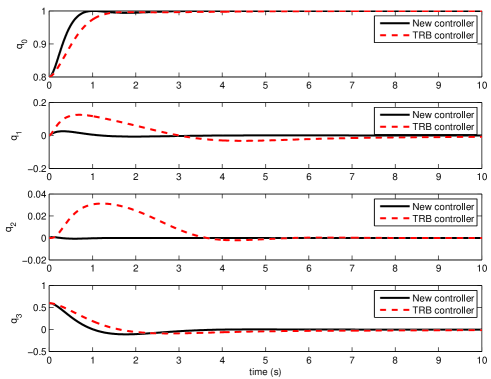
Figure 1: Quaternion trajectories for the new and TRB controllers with $Q(0)=\left[\begin{array}[]{c}0.8,\>0,\>0,\>0.6\end{array}\right]^{T}$

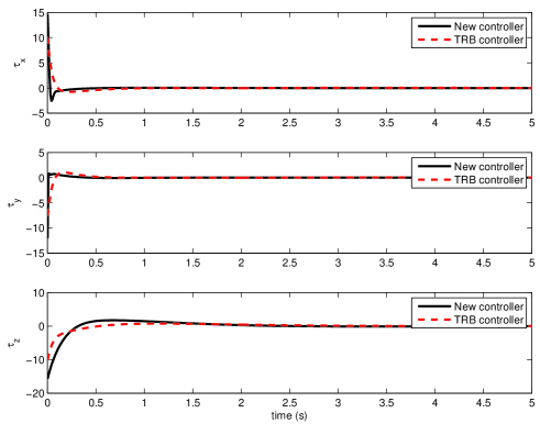
Figure 2: Applied torque for the new and TRB controllers

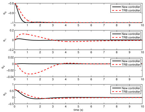
Figure 3: Quaternion trajectories for the new and TRB controllers with $Q(0)=\left[\begin{array}[]{c}-0.8,\>0,\>0,\>0.6\end{array}\right]^{T}$

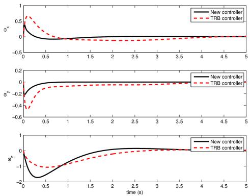
Figure 4: Angular velocity trajectories of the new and TRB controllers.

VI Conclusions

We have proposed an attitude stabilization controller for rigid body, in which neither the angular velocity nor the instantaneous measurements of the attitude are used in the feedback. This controller could be of great help (as main or backup controllers) in applications where prone-to-failure and expensive gyroscopes are used. When almost all existing solutions to this problem use the instantaneous attitude measurements, while it is well known that efficient attitude observer use the angular velocity to obtain an accurate results, our approach overcomes totally reconstructing the attitude. It mainly uses an auxiliary system that can be considered as an observer of the angular velocity using only the inertial measurements. The proposed controller doesn’t use the inertial fixed reference vectors, reduces the set of unstable equilibria of the closed loop dynamics with respect to previous proposed controller, provides an almost global stability of the desirable equilibrium and avoids the "unwinding phenomenon". In addition, it was shown that the set of control gains leading to a continuum of equilibria of the closed loop system is an algebraic variety of positive co-dimension, independently on the choice of the observed vectors. A non-linear optimal tuning method have been used to adjust properly the controller gains. We illustrated that the introduction of matrices gains gives a better results compared with existing work. The performances and effectiveness of the proposed solution were illustrated via simulation results.

gains	$l(\kappa(m))$	$u(\kappa(m))$
$\rho_{i}(i=1,2)$	0.01	30
$a_{i0}(i=1,2)$	0.0001	4
$a_{i1}(i=1,2)$	0.0001	2
$a_{i2}(i=1,2)$	0.0001	0.1
$\gamma_{ij}(i=1,2,j=1,2,3)$	0.01	50

Table I: Lower and upper limits

gains	ISE $g_{ise}(\kappa)=\int_{0}^{\infty}\left(\|\bar{q}\|^{2}+0.1\|\tau\|^{2}\right)dt$
$\rho_{i}(i=1,2)$	[22.5408, 1.7736 ]
$a_{1(j-1)}(j=1,2,3)$	[4, 2, 0.1]
$a_{2(j-1)}(j=1,2,3)$	[3.9672, 2, 0.1]
$\gamma_{1j}(j=1,2,3)$	[50, 28.7599, 0.0971]
$\gamma_{2j}(j=1,2,3)$	[1.8614, 1.7403, 13.9601]

Table II: Selected optimal gain values

parameters	values calculated with ISE criterion
$\Lambda_{1}$	diag([50, 28.7599, 0.0971])
$\Lambda_{2}$	diag([1.8614, 1.7403, 13.9601])
$A_{1}$	diag([550, 255.2727, 0.5838])
$A_{2}$	diag([11.4541, 10.6873, 102.7916])
$W_{rho}$	$\left[\begin{array}[]{ccc}24.3144&0&-1.7736\\ 0&26.0881&0\\ -1.7736&0&1.7736\end{array}\right]$
eigenvectors	$v_{\rho 1}=\pm\left[\begin{array}[]{c}0.0780\\ 0\\ 0.9970\end{array}\right]$
of $W_{rho}$	$v_{\rho 2}=\pm\left[\begin{array}[]{c}-0.9970\\ 0\\ 0.0780\end{array}\right]$, $v_{\rho 3}=\pm\left[\begin{array}[]{c}0\\ -1\\ 0\end{array}\right]$
eigenvalues	$\lambda_{\rho 1}=1.6349$, $\lambda_{\rho 2}=24.4531$
of $W_{rho}$	$\lambda_{\rho 3}=26.0881$

Table III: Gain matrices

References

- [1] M. Shuster, “A survey of attitude representations,” The Journal of the astronautical science, vol. 41, no. 4, pp. 439–517, October-December 1993.
- [2] J.-M. Pflimlina, P. Binettib, P. SouÚresa, T. Hamel, and D. Trouchet, “Modeling and attitude control analysis of a ducted-fan micro aerial vehicle,” Control Engineering Practice, vol. 18, pp. 209–218, 2010.
- [3] A.-M. Zou and K. D. Kumar, “Adaptive attitude control of spacecraft without velocity measurements using chebyshev neural network,” Acta Astronautica, vol. 66, pp. 769–779, 2010.
- [4] P. Castillo, P. Albertos, P. Garcia, and R. Lozano, “Simple real-time attitude stabilization of a quad-rotor aircraft with bounded signals,” in Proceedings of the 45th IEEE Conference on Decision & Control, December 2006, pp. 1533–1538.
- [5] J.-Y. Wen and K. Kreutz-Delgado, “The attitude control problem,” IEEE Transactions on Automatic Control, vol. 36, no. 10, pp. 1148 – 1162, October 1991.
- [6] R. Bayadi and R. N. Banavar, “Almost global attitude stabilization of a rigid body for both internal and external actuation schemes,” European Journal of Control, vol. 20, pp. 45–54, 2014.
- [7] T. Lee, “Robust adaptive attitude tracking on so(3) with an application to a quadrotor uav,” IEEE Transactions on Control Systems Technology, vol. 21, no. 5, pp. 1924–1930, 2013.
- [8] N. Chaturvedi, A. Sanyal, and N. McClamroch, “Rigid-body attitude control,” IEEE Control Systems Magazine, vol. 31, no. 3, pp. 30–51, June 2011.
- [9] R. Mahony, T. Hamel, and P. J.-M., “Nonlinear complementary filters on the special orthogonal group,” IEEE Transactions on Automatic Control, vol. 53 , Issue: 5, pp. 1203 – 1218, June 2008.
- [10] E. Fresk and G. Nikolakopoulos, “Full quaternion based attitude control for a quadrotor,” in European Control Conference (ECC), 2013.
- [11] Z. Zhu, Y. Xia, and M. Fu, “Adaptive sliding mode control for attitude stabilization with actuator saturation,” IEEE Transactions on Industrial Electronics, vol. 58, pp. 4898–4907, 2011.
- [12] C. G. Mayhew, R. G. Sanfelice, and A. R. Teel, “Robust global asymptotic attitude stabilization of a rigid body by quaternion-based hybrid feedback,” in Joint 48th IEEE Conference on Decision and Control and 28th Chinese Control Conference, 2009.
- [13] A. Tayebi and S. McGilvray, “Attitude stabilization of a vtol quadrotor aircraft,” IEEE Transactions On Control Systems Technology, vol. 14, no. 3, pp. 562–571, May 2006.
- [14] S. Joshi, A. Kelkar, and J.-Y. Wen, “Robust attitude stabilization of spacecraft using nonlinear quaternion feedback,” IEEE Transactions on Automatic Control, vol. 40, no. 10, pp. 1800–1803, 1995.
- [15] N. Nordkvist and A. Sanyal, “Attitude feedback tracking with optimal attitude state estimation,” in American Control Conference (ACC), 2010, pp. 2861–2866.
- [16] P. Pounds, T. Hamel, and R. Mahony, “Attitude control of rigid body dynamics from biased imu measurements,” in 46th IEEE Conference on Decision and Control, 2007, pp. 4620–4625.
- [17] A. Tayebi, S. McGilvray, A. Roberts, and M. Moallem, “Attitude estimation and stabilization of a rigid body using low-cost sensors,” in 46th IEEE Conference on Decision and Control, 2007, pp. 6424–6429.
- [18] P. Morin and C. Samson, “Time-varying exponential stabilization of a rigid spacecraft with two control torques,” IEEE Transactions on Automatic Control, vol. 42, pp. 528–534, 1997.
- [19] H. Krishnan, M. Reyhanoglu, and H. McClamroch, “Attitude stabilization of a rigid spacecraft using two control torques: A nonlinear control approach based on the spacecraft attitude dynamics,” Automatica, vol. 30, no. 06, pp. 1023–1027, 1994.
- [20] C. I. Byrnes and A. Isidori, “On the attitude stabilization of rigid spacecraft,” Automatica, vol. 27, pp. 87–95, 1991.
- [21] D. Thakur, “Adaptation, gyro-free stabilization, and smooth angular velocity observers for attitude tracking control applications,” Ph.D. dissertation, The University of Texas at Austin, August 2014.
- [22] L. Benziane, A. Benallegue, and A. Tayebi, “Attitude stabilization without angular velocity measurements,” in IEEE International Conference on Robotics & Automation (ICRA), 2014, pp. 3116–3121.
- [23] N. Filipe and P. Tsiotras, “Rigid body motion tracking without linear and angular velocity feedback using dual quaternions,” in European Control Conference (ECC), 2013.
- [24] A. Tayebi, A. Roberts, and A. Benallegue, “Inertial vector measurements based velocity-free attitude stabilization,” IEEE Transactions on Automatic Control, vol. 58, no. 11, pp. 2893–2898, November 2013.
- [25] B. Xiao, Q. Hu, and P. Shi, “Attitude stabilization of spacecrafts under actuator saturation and partial loss of control effectiveness,” IEEE Transactions On Control Systems Technology, vol. 21, pp. 2251–2263, 2013.
- [26] R. Schlanbusch, E. I. GrÞtli, A. Loria, and P. J. Nicklasson, “Hybrid attitude tracking of rigid bodies without angular velocity measurement,” Systems & Control Letters, vol. 61, pp. 595–601, 2012.
- [27] A. Tayebi, “A velocity-free attitude tracking controller for rigid spacecraft,” in 46th IEEE Conference on Decision and Control, 2007.
- [28] M. R. Akella, “Rigid body attitude tracking without angular velocity feedback,” Systems & Control Letters, vol. 42, pp. 321–326, 2001.
- [29] H. Wong, M. de Queiroz, and V. Kapila, “Adaptive tracking control using synthesized velocity from attitude measurements,” Automatica, vol. 37, no. 6, pp. 947 – 953, 2001.
- [30] A. Tayebi, “Unit quaternion-based output feedback for the attitude tracking problem,” IEEE Transactions on Automatic Control, vol. 53, no. 6, pp. 1516–1520, July 2008.
- [31] B. T. Costic, D. M. Dawson, M. S. d. Queiroz, and V. Kapila, “Quaternion-based adaptive attitude tracking controller without velocity measurements,” Journal of Guidance, Control, and Dynamics, vol. 24, no. 6, pp. 1214–1222, 2001.
- [32] P. Tsiotras, “Further passivity results for the attitude control problem,” IEEE Transactions on Automatic Control, vol. 43, no. 11, pp. 1597–1600, 1998.
- [33] F. Lizarralde and J. Wen, “Attitude control without angular velocity measurement: a passivity approach,” IEEE Transactions on Automatic Control, vol. 41, no. 3, pp. 468–472, 1996.
- [34] O. Egeland and J.-M. Godhavn, “Passivity-based adaptive attitude control of a rigid spacecraft,” IEEE Transactions on Automatic Control, vol. 39, pp. 842 – 846, Apr 1994.
- [35] S. P. Bhat and D. S. Bernstein, “A topological obstruction to continuous global stabilization of rotational motion and the unwinding phenomenon,” Systems & Control Letters, vol. 39, pp. 63–70, January 2000.
- [36] D. Hestenes, New Foundations for Classical Mechanics. Dordrecht: Kluwer Academic Publishers, 1999.
- [37] F. L. Markley and J. L. Crassidis, Fundamentals of Spacecraft Attitude Determination and Control. Microcosm Press and Springer, 2014.
- [38] L. Smith, Linear Algebra, 3rd ed., S.-V. N. Y. Inc., Ed., 1998.
- [39] F. Bullo and A. Lewis, Geometric Control of Mechanical Systems, I. Springer Science+Business Media, Ed., 2005.