Consumption investment optimization with Epstein-Zin utility in incomplete markets

Abstract.

In a market with stochastic investment opportunities, we study an optimal consumption investment problem for an agent with recursive utility of Epstein-Zin type. Focusing on the empirically relevant specification where both risk aversion and elasticity of intertemporal substitution are in excess of one, we characterize optimal consumption and investment strategies via backward stochastic differential equations. The supperdifferential of indirect utility is also obtained, meeting demands from applications in which Epstein-Zin utilities were used to resolve several asset pricing puzzles. The empirically relevant utility specification introduces difficulties to the optimization problem due to the fact that the Epstein-Zin aggregator is neither Lipschitz nor jointly concave in all its variables.

1. Introduction

Risk aversion and elasticity of intertemporal substitution (EIS) are two parameters describing two different aspects of preferences: risk aversion measures agent’s attitude toward risk, while EIS regulates agent’s willingness to substitute consumption over time. However commonly used time separable utilities force EIS to be the reciprocal of risk aversion, leading to a rich literature on asset pricing anomalies, such as the equity premium puzzle, the risk-free rate puzzle, the excess volatility puzzle, the credit spread puzzle, and etc.

Recursive utilities of Kreps-Porteus or Epstein-Zin type and their continuous-time analogue disentangle risk aversion and EIS, providing a framework to resolve aforementioned asset pricing puzzles, cf. [2] and [1] for the equity premium puzzle and the risk-free rate puzzle, [4] for the excess volatility puzzle, and [5] for the credit spread puzzle. All these studies require EIS $\psi$ to be larger than $1$ in order to match empirical observations. Bansal and Yaron [2] also empirically estimated $\psi$ to be around $1.5$. On the other hand, empirical evidence suggests that risk aversion $\gamma$ is in excess of $1$. It then follows from $\gamma>1$ and $\psi>1$ that $\gamma\psi>1$. Hence an agent with such a utility specification prefers early resolution of uncertainty (cf. [30] and [41]), therefore asks a sizeable risk premium to compensate future uncertainty in the state of economy.

Other than aforementioned utility specification, two other ingredients are also important in these asset pricing applications. First, investment opportunities in these models are driven by some state variables, which usually lead to unbounded market price of risk; for example, Heston model in [9], [26], and [31], Kim and Omberg model in [24] and [43]. Second, the first step in all these applications is to understand the superdifferential of the indirect utility for the representative agent, because it is the source to read out equilibrium risk-free rate and risk premium, cf. [2, Appendix]. Therefore, it is important to rigorously study the consumption investment problem simultaneously accounting these three ingredients: utility specification, models with unbounded market price of risk, and superdifferential of indirect utility. However, the following literature review shows that, such a study, in a continuous-time setting, was still missing from the literature. This paper fills this gap.

In the seminal paper by Duffie and Epstein [13], stochastic differential utilities (the continuous-time analogue of recursive utilities, cf. [28]) are assumed to have Lipschitz continuous aggregators. Hence the Epstein-Zin aggregator, which is non-Lipschitz, is excluded. Schroder and Skiadas [38] studied the case where $\theta=\frac{1-\gamma}{1-1/\psi}$ is positive. However the empirically revelent parameter specification $\gamma,\psi>1$ leads to $\theta<0$. Kraft, Seifried, and Steffensen [29] studied incomplete market models with unbounded market price of risk, however their assumption on $\gamma$ and $\psi$ (cf. Equation (H) therein) excludes the case $\gamma>1$ and $\psi>1$.

Regarding market models, Schroder and Skiadas [38] studied a complete market with bounded market price of risk. Schroder and Skiadas [39, Section 5.6], Chacko and Viceira [9] both considered incomplete markets and Epstein-Zin utility with unit EIS. Chacko and Viceira [9], Kraft, Seifried, and Steffensen [29] studied a market model whose investment opportunities are driven by a square root process, leading to unbounded market price of risk.

Regarding the superdifferential of indirect utility, its form can be obtained by a heuristic calculation using the utility gradient approach, cf. [15]. However, rigorous verification needs the aggregator to satisfy a Lipschitz growth condition (cf. [13] and [15]), or joint concavity in both consumption and utility variables (cf. [16]). As we shall see later, when $\gamma>1$ and $\psi>1$, the Epstein-Zin aggregator is neither Lipschitz continuous nor joint concave. On the other hand, for Epstein-Zin utility with $\theta>0$, Schroder and Skiadas [38] verified the superdifferential via an integrability condition (cf. [38, Lemma 2]) and the property that the sum of deflated wealth process and integral of deflated consumption stream is a supermartingale for arbitrary admissible strategy, and is a martingale for the optimal strategy (cf. [38, Equation (1)]). Both these two conditions are verified in [38, Theorem 2 and 4] for complete market models with bounded market price of risk.

In this paper, we analyze a consumption investment problem for an agent with Epstein-Zin utility with $\gamma,\psi>1$ and a bequest utility at a finite time horizon. This agent invests in an incomplete market whose investment opportunities are driven by a multi-variate state variable. Rather than the Campbell-Shiller approximation, which is widely applied for utilities with non-unit EIS, we study the exact solution. As illustrated in [29, Section 6], there can be a sizeable deviation of the Campbell-Shiller approximation from the exact solution, highlighting the importance of exact solution.

A similar problem has also been studied recently by Kraft, Seiferling, and Seifried [27]. In this paper, the relation between $\gamma$ and $\psi$ in [29] is removed, all configurations of $\gamma$ and $\psi$ are considered including the $\gamma,\psi>1$ case. Verification result is obtained following the utility gradient approach in [15] and [38], complemented by a recent note of Seiferling and Seifried [40] for the $\gamma,\psi>1$ case. Nevertheless, [27] focuses on models with bounded market price of risk (cf. Assumptions (A1) and (A2) therein). This excludes models, such as Heston model and Kim-Omberg models, which are widely used in aforementioned asset pricing applications. Comparing to [27] and all other aforementioned existing results, the current paper extends the previous literature in three respects.

First, in contrast to the utility gradient approach, the verification result is obtained by comparison results for backward stochastic differential equations (BSDE). Rather than employing the dynamic programming method as in [29] and [27], optimal consumption and investment strategies are represented by a BSDE solution, cf. Theorem 2.14 below. Extending techniques of Hu, Imkeller, and Müller [20] and Cheridito and Hu [11], who studied optimal consumption investment problems for time separable utilities, we verify the candidate optimal strategies for Epstein-Zin utility.

Second, our method is designed for market models with unbounded market value of risk. Utilizing Lyapunov functions, borrowed from [42, Chapter 10], we prove in Lemma B.2 below that certain exponential local martingale is martingale, which is a key component of our verification argument.

Third, we verify the superdifferential of indirect utility. Comparing to [38], the integrability condition in Lemma 2 therein is satisfied when $\gamma,\psi>1$. For the second step of verification in [38] and [27], it requires that the sum of deflated wealth process and integral of deflated consumption stream is a supermartingale for any admissible strategy, and is a martingale for the optimal one. We obtain this property (see Theorem 2.16 below) as a by-product of our verification result. This result is established for models with unbounded market price of risk, hence meets demands coming from aforementioned applications on asset pricing puzzles.

Our general results in Section 2 are specialized to two examples in Section 3. There numeric results reveal an interesting phenomenon. As time horizon goes to infinity, convergence of the finite horizon solution to its stationary long run limit is very slow when $\psi>1$. Figure 2 shows that this convergence takes at least $60$ years in an empirically revelent utility and market setting. Moreover, the convergence is sensitive to the time discounting parameter: it is much slower when the discounting parameter decreases slightly. This is in contrast to the $\psi<1$ case, where the convergence is much faster (around $20$ years) and is less sensitive to the time discounting parameter. This observation implies that, in the $\psi>1$ setting, the finite horizon optimal strategy can be far away from its infinite horizon analogue, even when we consider a lifelong consumption investment problem.

The remaining of this paper is organized as follows. After Epstein-Zin utility is introduced in Section 2.1, the consumption investment problem is introduced and main results are presented in Section 2.2. Then main results are specialized in two examples in Section 3, where general assumptions of main results are verified under explicit parameters restrictions, which include many empirically relevant cases. All proofs are postponed to appendices.

2. Main results

2.1. Epstein-Zin preferences

We work on a filtered probability space $(\Omega,(\mathcal{F}_{t})_{0\leq t\leq T},\mathcal{F},\mathbb{P})$. Here $(\mathcal{F}_{t})_{0\leq t\leq T}$ is the augmented filtration generated by a $k+n-$dimensional Wiener process $B=(W,W^{\bot})$, where $W$ and $W^{\bot}$ are the first $k$ and the last $n$ components, respectively, and satisfies the usual hypotheses of right-continuity and completeness.

Let $\mathcal{C}$ be the class of nonnegative progressively measurable processes on $[0,T]$. For $c\in\mathcal{C}$ and $t<T$, $c_{t}$ stands for the consumption rate at $t$ and $c_{T}$ represents a lump sum consumption at $T$. We consider an agent whose preference over $\mathcal{C}-$valued consumption streams is described by a continuous time stochastic differential utility of Kreps-Porteus or Epstein-Zin type. To describe this preference, let $\delta>0$ represent the discounting rate, $0<\gamma\neq 1$ be the relative risk aversion, and $0<\psi\neq 1$ be the EIS. We focus on the $\gamma>1$ case. In this case, define the Epstein-Zin aggregator $f:[0,\infty)\times(-\infty,0]\rightarrow\mathbb{R}$ via

(2.1) $$f(c,v):=\delta\,\frac{(1-\gamma)v}{1-\frac{1}{\psi}}\left[\left(\frac{c}{((1-\gamma)v)^{\frac{1}{1-\gamma}}}\right)^{1-\frac{1}{\psi}}-1\right].$$

This is a standard parametrization used, for instance, in [12]. Given a bequest utility function $U(c)=c^{1-\gamma}/(1-\gamma)$, the Epstein-Zin utility over the consumption stream $c\in\mathcal{C}$ on a finite time horizon $T$ is a process $V^{c}$ which satisfies

(2.2) $$V^{c}_{t}=\mathbb{E}_{t}\left[\int_{t}^{T}f(c_{s},V_{s}^{c})\,ds+U(c_{T})\right],\quad\text{ for all }t\in[0,T],$$

where $\mathbb{E}_{t}$ stands for $\mathbb{E}[\cdot|\mathcal{F}_{t}]$.

Remark 2.1.

Epstein-Zin utility generalizes the standard time separable utility with constant relative risk aversion. Indeed, when $\gamma=1/\psi$, the aggregator reduces to $f(c,v)=\delta\frac{c^{1-\gamma}}{1-\gamma}-\delta v$. Then (2.2) with $t=0$ can be represented explicitly as the standard time separable utility:

$$V_{0}^{c}=\mathbb{E}\left[\int_{0}^{T}\delta e^{-\delta s}\frac{c_{s}^{1-\gamma}}{1-\gamma}\,ds+e^{-\delta T}U(c_{T})\right].$$

As discussed in introduction, we are interested in the empirical relevant case where $\gamma>1$ and $\psi>1$. In this case, $\gamma=1/\psi$ is violated, hence (2.2) is not time separable.

When $c$ follows a diffusion, the existence of $V^{c}$ was established by Duffie and Lions [14] via partial differential equation techniques. We work with a non-Markovian setting and construct $V^{c}$ via the following BSDE:

(2.3) $$V_{t}^{c}=U(c_{T})+\int_{t}^{T}f(c_{s},V^{c}_{s})\,ds-\int_{t}^{T}Z^{c}_{s}\,dB_{s},\quad 0\leq t\leq T.$$

Denote

$$\theta:=\frac{1-\gamma}{1-\frac{1}{\psi}}.$$

When $\gamma,\psi>1$, $\theta<0$. The generator in (2.3) is

$$f(c,v)=\delta\frac{c^{1-\frac{1}{\psi}}}{1-\frac{1}{\psi}}\left((1-\gamma)v\right)^{1-\frac{1}{\theta}}-\delta\theta v.$$

Then $f$ has super-linear growth in $v$ when $\theta<0$. Therefore the BSDE (2.3) does not have a Lipschitz generator. Nevertheless, consider $(Y_{t},Z_{t}):=e^{-\delta\theta t}(1-\gamma)(V^{c}_{t},Z^{c}_{t})$ and the following transformed BSDE:

(2.4) $$Y_{t}=e^{-\delta\theta T}c_{T}^{1-\gamma}+\int_{t}^{T}F(s,c_{s},Y_{s})\,ds-\int_{t}^{T}Z_{s}dB_{s},\quad\text{ where }F(t,c_{t},y):=\delta\theta e^{-\delta t}c_{t}^{1-\frac{1}{\psi}}y^{1-\frac{1}{\theta}}.$$

When $\theta<0$, the generator $F$ in (2.4) satisfies the monotonicity condition, i.e., $y\mapsto F(t,c_{t},y)$ is decreasing. This allows us to establish the existence and uniqueness of solutions to (2.3), hence define $V^{c}$ satisfying (2.2).

Let us introduce the set of admissible consumption streams as

$$\mathcal{C}_{a}:=\left\{c\in\mathcal{C}\,:\,\mathbb{E}\left[\int_{0}^{T}e^{-\delta s}c_{s}^{1-\frac{1}{\psi}}ds\right]<\infty\text{ and }\mathbb{E}\left[c_{T}^{1-\gamma}\right]<\infty\right\}.$$

Proposition 2.2.

Suppose $\gamma,\psi>1$ and $c\in\mathcal{C}_{a}$. Then (2.4) admits a unique solution $(Y,Z)$ in which $Y$ is continuous, strictly positive, and is of class $D$, $\int_{0}^{T}|Z_{t}|^{2}dt<\infty$ a.s.. Moreover, $V^{c}_{t}:=e^{\delta\theta t}Y_{t}/(1-\gamma)$, $t\in[0,T]$, satisfies (2.2).

Remark 2.3.

When a BSDE satisfies the monotonicity condition, it is customary to assume its terminal condition to be square integrable, cf. [34, Theorem 2.2]. However this imposes unnecessary restrictions for later described utility maximization problem, in the sense that the bequest utility needs to be square integrable to define the associated Epstein-Zin utility. Therefore, Proposition 2.2 only asks for the terminal condition to be an integrable random variable.

Having defined $V^{c}_{0}$, we expect that, as a utility functional, $\mathcal{C}_{a}\ni c\mapsto V^{c}_{0}$ is concave. This would follow from the standard argument when $f(c,v)$ is jointly concave in $c$ and $v$, cf. [13, Proposition 5]. However, calculation shows that $f$ in (2.1) is not jointly concave when $\gamma>1$ and $\psi>1$. Nevertheless, utilizing an orderly equivalent transformation of $V^{c}_{0}$, introduced in [13, Example 3], the following proposition confirms the concavity of $c\mapsto V^{c}_{0}$.

Let us define $(\mathbb{Y},\mathbb{Z}):=(Y^{1/\theta},\frac{1}{\theta}Y^{1/\theta-1}Z)/(1-\frac{1}{\psi})$. Calculation shows that $(\mathbb{Y},\mathbb{Z})$ satisfies

(2.5) $$\mathbb{Y}_{t}=e^{-\delta T}\frac{c_{T}^{1-\frac{1}{\psi}}}{1-\frac{1}{\psi}}+\int_{t}^{T}\left[\delta e^{-\delta s}\frac{c_{s}^{1-\frac{1}{\psi}}}{1-\frac{1}{\psi}}+\frac{1}{2}(\theta-1)\frac{\mathbb{Z}^{2}_{s}}{\mathbb{Y}_{s}}\right]\,ds-\int_{t}^{T}\mathbb{Z}_{s}dB_{s}.$$

Observe that the generator of (2.5) is now jointly concave in $(c,\mathbb{Y},\mathbb{Z})$ when $\theta<1$.

Proposition 2.4.

When $\gamma,\psi>1$, for any $c,\tilde{c}\in\mathcal{C}_{a}$, and $\alpha\in[0,1]$, if $\alpha C+(1-\alpha)\tilde{c}\in\mathcal{C}_{a}$, then

$$\alpha V_{0}^{c}+(1-\alpha)V^{\tilde{c}}_{0}\leq V^{\alpha c+(1-\alpha)\tilde{c}}_{0}.$$

Remark 2.5.

The integrability condition in $\mathcal{C}_{a}$ does not implies the convexity of $\mathcal{C}_{a}$. Indeed, since $\psi>1$, $\mathbb{E}[\int_{0}^{T}e^{-\delta s}\beta_{s}^{1-\frac{1}{\psi}}ds]<\infty$ for both $\beta=c$ and $\tilde{c}$ does not imply the same integrability for $\alpha c+(1-\alpha)\tilde{c}$. However Proposition 2.4 implies the concavity of $c\mapsto V^{c}$ on any convex subset of $\mathcal{C}_{a}$, for example, $\mathcal{C}_{a}^{1}=\{c\in\mathcal{C}_{a}\,:\,\mathbb{E}[\int_{0}^{T}e^{-\delta s}c_{s}ds]<\infty\}$.

2.2. Consumption investment optimization

Having established the existence of Epstein-Zin utility in the previous section, we consider an optimal consumption investment problem for an agent with such a utility.

Consider a model of a financial market with a risk free asset $S^{0}$ and risky assets $S=(S^{1},\dots,S^{n})$ with dynamics

(2.6) $$\begin{split}dS^{0}_{t}&=S^{0}_{t}r(X_{t})dt,\\ dS_{t}&=\text{diag}(S_{t})\left[\left(r(X_{t})1_{n}+\mu(X_{t})\right)dt+\sigma(X_{t})dW^{\rho}_{t}\right],\end{split}$$

where $\text{diag}(S)$ is a diagonal matrix with elements of $S$ on the diagonal, $1_{n}$ is a $n-$dimensional vector with every entry $1$. Given a correlation function $\rho:\mathbb{R}^{k}\rightarrow\mathbb{R}^{n\times k}$ and $\rho^{\bot}:\mathbb{R}^{k}\rightarrow\mathbb{R}^{n\times n}$, satisfying $\rho\rho^{\prime}+\rho^{\bot}(\rho^{\bot})^{\prime}=1_{n\times n}$ (the $n\times n$ identity matrix), $W^{\rho}:=\int_{0}^{\cdot}\rho(X_{s})dW_{s}+\int_{0}^{\cdot}\rho^{\bot}(X_{s})dW^{\bot}_{s}$ defines a $n-$dimensional Brownian motion. In (2.6), $X$ is a $E-$valued state variable satisfying

(2.7) $$dX_{t}=b(X_{t})dt+a(X_{t})dW_{t},\quad X_{0}=x\in E.$$

Here $E\subseteq\mathbb{R}^{k}$ is an open domain, $r:E\rightarrow\mathbb{R}$, $\mu:E\rightarrow\mathbb{R}^{n}$, $\sigma:E\rightarrow\mathbb{R}^{n\times n}$, $b:E\rightarrow\mathbb{R}^{k}$, and $a:E\rightarrow\mathbb{R}^{k\times k}$. These model coefficients satisfy following assumptions.

Assumption 2.6.

$r$, $\mu$, $\sigma$, $b$, $a$, and $\rho$ are all locally Lipschitz in $E$; $A:=aa^{\prime}$ and $\Sigma=\sigma\sigma^{\prime}$ are positive definite in any compact subdomain of $E$; $r+\frac{1}{2\gamma}\mu^{\prime}\Sigma^{-1}\mu$ is bounded from below on $E$, moreover, dynamics of (2.7) does not hit boundary of $E$ in finite time.

In the previous assumption, local Lipschitz continuity of coefficients and the nonexplosion assumption combined imply that (2.7) admits a unique $E$-valued strong solution $X$. When the interest rate $r$ is bounded from below, due to $\tfrac{1}{2\gamma}\mu^{\prime}\Sigma^{-1}\mu\geq 0$, $r+\frac{1}{2\gamma}\mu^{\prime}\Sigma^{-1}\mu$ is bounded from below as well.

An agent, whose preference is described by an Epstein-Zin utility, invests in this financial market. Given an initial wealth $w$, an investment strategy $\pi$, and a consumption rate $c$, the wealth of the agent follows

(2.8) $$d\mathcal{W}^{\pi,c}_{t}=\mathcal{W}^{\pi,c}_{t}\left[(r_{t}+\pi^{\prime}_{t}\mu_{t})dt+\pi^{\prime}_{t}\sigma_{t}dW^{\rho}_{t}\right]-c_{t}dt,\quad\mathcal{W}^{\pi,c}_{0}=w.$$

Throughout the paper, $r_{t},\mu_{t},\rho_{t},\sigma_{t}$ stand for $r(X_{t}),\mu(X_{t}),\rho(X_{t})$, and $\sigma(X_{t})$, respectively, and the superscript $(\pi,c)$ is sometimes suppressed on $\mathcal{W}$ to simplify notation. A pair of investment strategy and consumption stream $(\pi,c)$ is admissible if $c\in\mathcal{C}_{a}$ and its associated wealth process is nonnegative. The agent aims to maximize her utility $V^{c}_{0}$.

We will further restrict admissible strategies to a permissible set. But let us first characterize the optimal value process via a heuristic argument. By homothetic property of Epstein-Zin utility, we speculate that utility evaluated at the optimal strategy has the following decomposition:

(2.9) $$V^{*}_{t}=\frac{\mathcal{W}_{t}^{1-\gamma}}{1-\gamma}e^{Y_{t}},\quad t\in[0,T],$$

where $Y$ satisfies the following BSDE

(2.10) $$Y_{t}=\int_{t}^{T}H(s,Y_{s},Z_{s},Z^{\bot}_{s})\,ds-\int_{t}^{T}Z_{s}\,dW_{s}-\int_{t}^{T}Z^{\bot}_{s}dW^{\bot}_{s}.$$

Let us determine the generator $H$ in what follows. Parameterizing $c$ by $c=\tilde{c}\,\mathcal{W}$, the wealth process satisfies

$$\frac{d\mathcal{W}_{t}}{\mathcal{W}_{t}}=(r_{t}-\tilde{c}_{t}+\pi^{\prime}_{t}\mu_{t})dt+\pi^{\prime}_{t}\sigma_{t}dW^{\rho}_{t}.$$

We expect from the standard dynamic programming principle that $\frac{\mathcal{W}_{t}^{1-\gamma}}{1-\gamma}e^{Y_{t}}+\int_{0}^{t}f\left(c_{s},\frac{\mathcal{W}^{1-\gamma}_{s}}{1-\gamma}e^{Y_{s}}\right)ds$ is a supermartingale martingale for arbitrary strategy, and is a martingale for the optimal strategy. Let us calculate the drift of the previous process. Calculation shows that

$$d\mathcal{W}^{1-\gamma}_{t} =\mathcal{W}_{t}^{1-\gamma}\left[(1-\gamma)(r_{t}-\tilde{c}_{t}+\pi^{\prime}_{t}\mu_{t})-\frac{\gamma(1-\gamma)}{2}\pi^{\prime}_{t}\Sigma_{t}\pi_{t}\right]dt+(1-\gamma)\mathcal{W}^{1-\gamma}_{t}\pi^{\prime}_{t}\sigma dW^{\rho}_{t}.$$

$$de^{Y_{t}} =e^{Y_{t}}\left(-H(t,Y_{t},Z_{t},Z^{\bot}_{t})+\frac{1}{2}Z_{t}Z^{\prime}_{t}+\frac{1}{2}Z^{\bot}_{t}(Z^{\bot}_{t})^{\prime}\right)dt+e^{Y_{t}}\left(Z_{t}dW_{t}+Z^{\bot}_{t}dW^{\bot}_{t}\right).$$

Therefore, the drift of $\frac{\mathcal{W}_{s}^{1-\gamma}}{1-\gamma}e^{Y_{t}}+\int_{0}^{t}f\left(c_{s},\frac{\mathcal{W}_{s}^{1-\gamma}}{1-\gamma}e^{Y_{s}}\right)ds$ reads (the time subscript is omitted to simplify notation)

(2.11) $$\begin{split}\frac{\mathcal{W}^{1-\gamma}}{1-\gamma}e^{Y}&\left\{(1-\gamma)r-\delta\theta+\frac{1}{2}ZZ^{\prime}+\frac{1}{2}Z^{\bot}(Z^{\bot})^{\prime}+\left[-(1-\gamma)\tilde{c}+\delta\theta e^{-\frac{1}{\theta}Y}\tilde{c}^{1-\frac{1}{\psi}}\right]\right.\\ &\left.+\left[-\frac{\gamma(1-\gamma)}{2}\pi^{\prime}\Sigma\pi+(1-\gamma)\pi^{\prime}(\mu+\sigma\rho Z+\sigma\rho^{\bot}Z^{\bot})\right]-H(\cdot,Y,Z,Z^{\bot})\right\}.\end{split}$$

We expect that the drift above is negative for arbitrary $(\pi,\tilde{c})$ and is zero for the optimal strategy. Therefore, the generator $H$ for (2.10) can be obtained by taking supremum on $\pi$ and $\tilde{c}$ in the previous drift and setting it to be zero. Following this direction, we notice that the randomness in $H$ comes only from $X$, which is driven by $W$, moreover, the terminal condition of (2.10) is zero. As a result, $Z^{\bot}$ is necessarily zero. Therefore, we can reduce (2.10) to

(2.12) $$Y_{t}=\int_{t}^{T}H(s,Y_{s},Z_{s})ds-\int_{t}^{T}Z_{s}dW_{s},$$

where $H$ is given by

(2.13) $$\begin{split}H(t,y,z)=&(1-\gamma)r_{t}-\delta\theta+\frac{1}{2}zz^{\prime}+\inf_{\tilde{c}}\left[-(1-\gamma)\tilde{c}+\delta\theta e^{-\frac{1}{\theta}y}{\tilde{c}}^{1-\frac{1}{\psi}}\right]\\ &+\inf_{\pi}\left[-\frac{\gamma(1-\gamma)}{2}\pi^{\prime}\Sigma_{t}\pi+(1-\gamma)\pi^{\prime}(\mu_{t}+\sigma_{t}\rho_{t}z^{\prime})\right]\\ =&\frac{1}{2}zM_{t}z^{\prime}+\frac{1-\gamma}{\gamma}\mu^{\prime}_{t}\Sigma^{-1}_{t}\sigma_{t}\rho_{t}z^{\prime}+\theta\frac{\delta^{\psi}}{\psi}e^{-\frac{\psi}{\theta}y}+h_{t}-\delta\theta.\end{split}$$

Here, suppressing the subscript $t$,

$$\Sigma:=\sigma\sigma^{\prime}(X),\quad M:=1_{k\times k}+\frac{1-\gamma}{\gamma}\rho^{\prime}\sigma^{\prime}\Sigma^{-1}\sigma\rho(X),\quad\text{ and }\quad h:=(1-\gamma)r(X)+\frac{1-\gamma}{2\gamma}\mu^{\prime}\Sigma^{-1}\mu(X),$$

where $1_{k\times k}$ is the $k\times k$-identity matrix. Recall from Assumption 2.6 that $r+\frac{1}{2\gamma}\mu^{\prime}\Sigma^{-1}\mu$ is bounded from below. Therefore $\gamma>1$ implies that there exists a positive constant $h_{max}$ such that $h\leq h_{max}$ on $E$. The infimum in (2.13) are due to $\gamma>1$, and they are attained at

(2.14) $$\pi^{*}_{t}=\frac{1}{\gamma}\Sigma^{-1}_{t}\left(\mu_{t}+\sigma_{t}\rho_{t}Z^{\prime}_{t}\right)\quad\text{ and }\quad\frac{c^{*}_{t}}{\mathcal{W}_{t}^{*}}=\tilde{c}^{*}_{t}=\delta^{\psi}e^{-\frac{\psi}{\theta}Y_{t}},\quad t\in[0,T),$$

where $\mathcal{W}^{*}$ is the wealth process associated to the strategy $(\pi^{*},c^{*})$. Therefore $\pi^{*}$ and $c^{*}$ are candidate optimal strategies.

Coming back to (2.12), even though the generator $H$ has an exponential term in $y$ and a quadratic term in $z$, the parameter specification $\gamma,\psi>1$ allows us to derive a priori bounds on $Y$. In particular, $Y$ is bounded from above by a constant. Meanwhile, since the quadratic term of $z$ in $H$ will be shown to be nonnegative, the lower bound of $Y$ can be obtained by studying a BSDE whose generator does not contain this quadratic term. As a result, a solution to (2.12) can be constructed under the following mild integrability conditions.

Assumption 2.7.

 

1. $\frac{d\overline{\mathbb{P}}}{d\mathbb{P}}=\mathcal{E}\left(\int\frac{1-\gamma}{\gamma}\mu^{\prime}\Sigma^{-1}\sigma\rho(X_{s})dW_{s}\right)_{T}$ defines a probability measure $\overline{\mathbb{P}}$ equivalent to $\mathbb{P}$;

2. $\mathbb{E}^{\overline{\mathbb{P}}}\left[\int_{0}^{T}h(X_{s})ds\right]>-\infty$.

Here $\mathcal{E}(\int\alpha_{s}dW_{s})_{T}:=\exp\left(-\frac{1}{2}\int_{0}^{T}|\alpha_{s}|^{2}ds+\int_{0}^{T}\alpha_{s}dW_{s}\right)$ denotes the stochastic exponential for $\int_{0}^{T}\alpha_{s}dW_{s}$.

Remark 2.8.

Since the generator $H$ contains a linear term in $z$, it is natural to apply Girsanov theorem. Assumption 2.7 i) allows us to do this and write (2.12) under $\overline{\mathbb{P}}$. This assumption can be checked by explosion criteria; see Section 3 for examples. In ii), the standard exponential moment condition in [6] is avoid, due to the special structure of $H$: the quadratic term in $z$ is nonnegative, and $H(\cdot,0,0)$ is bounded from above by $h_{max}-\delta\theta$.

Proposition 2.9.

When $\gamma,\psi>1$, let Assumption 2.7 hold. Then (2.12) admits a solution $(Y,Z)$ such that, for any $t\in[0,T]$,

(2.15) $$\mathbb{E}^{\overline{\mathbb{P}}}_{t}\left[\int_{t}^{T}h(X_{s})\,ds\right]-\delta\theta(T-t)+\theta\frac{\delta^{\psi}}{\psi}e^{(\delta\psi-\frac{\psi}{\theta}h_{\max})T}(T-t)\leq Y_{t}\leq-\delta\theta(T-t)+\log\mathbb{E}^{\overline{\mathbb{P}}}_{t}\left[\exp{\left(\int_{t}^{T}h(X_{s})\,ds\right)}\right],$$

and $\mathbb{E}[\int_{0}^{T}|Z_{s}|^{2}ds]<\infty$. In particular, since $h\leq h_{max}$, $Y$ is bounded from above by $(h_{max}-\delta\theta)T$.

Having constructed $(Y,Z)$, the strategies $(\pi^{*},c^{*})$ in (2.14) are well defined. To verify their optimality, we need to further restrict the admissible strategies to a permissible set: $(\pi,c)$ is permissible if $c\in\mathcal{C}_{a}$ and $(\mathcal{W}^{\pi,c})^{1-\gamma}e^{Y}$ is of class $D$ on $[0,T]$.

To verify the optimality for $(\pi^{*},c^{*})$, let us introduce an operator $\mathfrak{F}$. For $\phi\in C^{2}(E)$,

(2.16) $$\mathfrak{F}[\phi]:=\frac{1}{2}\sum_{i,j=1}^{k}A_{ij}\partial^{2}_{x_{i}x_{j}}\phi+\left(b+\frac{1-\gamma}{\gamma}a\rho^{\prime}\sigma^{\prime}\Sigma^{-1}\mu\right)^{\prime}\nabla\phi+\frac{1}{2}\nabla\phi^{\prime}aMa^{\prime}\nabla\phi+h,$$

where the dependence on $x$ is suppressed on both sides. The function $\phi$ in the following assumption is called a Lyapunov function. Its existence facilities proving certain exponential local martingale is in fact martingale, hence verifying optimality of the candidate strategies. This strategy has been applied to portfolio optimization problems for time separable utilities, cf. [18] and [37].

Assumption 2.10.

There exists $\phi\in C^{2}(E)$ such that

1. $\lim_{n\rightarrow\infty}\inf_{x\in E\setminus E_{n}}\phi(x)=\infty$, where $(E_{n})_{n}$ is a sequence of open domains in $E$ satisfying $\cup_{n}E_{n}=E$, $\overline{E}_{n}$ compact, and $\overline{E}_{n}\subset E_{n+1}$, for each $n$;

2. $\mathfrak{F}[\phi]$ is bounded from above on $E$.

The final assumption before the main results imposes an integrability assumption on the market price of risk $\lambda$. This ensures $\mathbb{E}\left[\int_{0}^{T}e^{-\delta s}(c_{s}^{*})^{1-1/\psi}ds\right]<\infty$, hence the admissibility for the candidate optimal consumption stream $c^{*}$.

Assumption 2.11.

There exists $\lambda:E\rightarrow\mathbb{R}^{n}$ which satisfies $\mu=\sigma\lambda$ and defines a local martingale measure $\mathbb{Q}^{0}$ for the discounted asset price via $d\mathbb{Q}^{0}/d\mathbb{P}=\mathcal{E}(\int-\lambda^{\prime}_{s}dW^{\rho}_{s})_{T}$. Moreover

(2.17) $$\mathbb{E}^{\mathbb{Q}^{0}}\left[e^{(\psi-1)\int_{0}^{T}r_{+}(X_{s})ds}\mathcal{E}\left(\int\lambda^{\prime}(X_{s})\,dW^{0}_{s}\right)_{T}^{\psi}\right]<\infty,$$

where $W^{0}:=W^{\rho}+\int_{0}^{\cdot}\lambda_{s}ds$ is a $\mathbb{Q}^{0}-$Brownian motion and $r_{+}=\max\{r,0\}$.

Remark 2.12.

The previous assumption is stated under the minimal martingale measure $\mathbb{Q}^{0}$ (cf. [17]). A careful examination of Lemma B.4 shows that this assumption can be replaced by any local martingale measure $\mathbb{Q}$ such that $\mathbb{E}^{\mathbb{Q}}[\exp((\psi-1)\int_{0}^{T}r_{+}(X_{s})ds)(d\mathbb{P}/d\mathbb{Q})^{\psi}]<\infty$.

Remark 2.13.

When $r$ and $\lambda$ are bounded, Assumption 2.11 holds automatically and Assumption 2.10 is not needed, even for non-Markovian models. Indeed, Assumption 2.10 is used to prove the stochastic exponential in Lemma B.2 below is a martingale. When $r$ and $\lambda$ are bounded, $h$ is bounded, hence $H(\cdot,0,0)$ is bounded as well. Therefore, (2.15) implies that $Y$ is bounded, and $\int_{0}^{\cdot}Z_{s}dW_{s}$ is a BMO-martingale, cf. eg. [33, Lemma 3.1]. Then the stochastic exponential in Lemma B.2 can be proved as a martingale directly. However many models do not have bounded market value of risk. Therefore we retain Assumptions 2.10 and 2.11 in their general forms. These conditions impose some market conditions. In particular, for Markovian models, these conditions will be specified as explicit parameter restrictions in two examples in Section 3 below.

Now we are ready to state our first main result.

Theorem 2.14.

When $\gamma,\psi>1$, let Assumptions 2.6, 2.7, 2.10, and 2.11 hold. Then $\pi^{*}$ and $c^{*}$ in (2.14) maximize the Epstein-Zin utility among all permissible strategies. Moreover, the optimal Epstein-Zin utility is given by

$$\frac{w^{1-\gamma}}{1-\gamma}e^{Y_{0}}.$$

The second main result below focuses on the superdifferential of indirect utility. Let us first define the optimal value process

(2.18) $$V^{*}_{t}:=\frac{(\mathcal{W}^{*}_{t})^{1-\gamma}}{1-\gamma}e^{Y_{t}},\quad t\in[0,T],$$

where $\mathcal{W}^{*}$ is the optimal wealth process and $Y$ comes from Proposition 2.9. Schroder and Skiadas [38] conjectured in Assumption C3 therein that the superdifferential is

(2.19) $$D^{*}_{t}=w^{\gamma}e^{-Y_{0}}\exp\left[\int_{0}^{t}\partial_{v}f(c^{*}_{s},V^{*}_{s})ds\right]\partial_{c}f(c^{*}_{t},V^{*}_{t}),\quad t\in[0,T].$$

The constant $w^{\gamma}e^{-Y_{0}}$ in (2.19) normalizes $D^{*}_{0}$ to be $1$. Indeed, combining (2.1), (2.14) and (2.18), calculation shows that

(2.20) $$D^{*}_{t} = w^{\gamma}e^{-Y_{0}}\exp\left[\int_{0}^{t}\delta(\theta-1)((1-\gamma)V^{*}_{s})^{-\frac{1}{\theta}}(c^{*}_{s})^{1-\frac{1}{\psi}}ds-\delta\theta t\right]\delta((1-\gamma)V^{*}_{t})^{1-\frac{1}{\theta}}(c^{*}_{t})^{-\frac{1}{\psi}}$$

$$= \exp\left[\int_{0}^{t}(\theta-1)\delta^{\psi}e^{-\frac{\psi}{\theta}Y_{s}}ds-\delta\theta t\right]\frac{(\mathcal{W}_{t}^{\pi^{*}})^{-\gamma}e^{Y_{t}}}{w^{-\gamma}e^{Y_{0}}}.$$

Therefore the previous identity implies that $D^{*}_{0}=1$ and $D^{*}$ is nonnegative.

In [38, Theorems 2 and 4], $D^{*}$ is confirmed to be the superdifferential when the market is complete with bounded market price of risk. This is proved using an integrability assumption in [38, Lemma 2], together with the property that $\mathcal{W}D^{*}+\int_{0}^{\cdot}D^{*}_{s}c_{s}ds$ is a supermartingale for arbitrary strategy and is a martingale for the optimal strategy. The integrability assumption in [38, Lemma 2] is satisfied in our case. Indeed, (2.20) shows that $\partial_{v}f(c^{*},V^{*})=(\theta-1)\delta^{\psi}e^{-\frac{\psi}{\theta}Y}-\delta\theta$, which is bounded due to $\theta<0$ and $Y$ is bounded from above. Now the following result confirms aforementioned property for $\mathcal{W}D^{*}+\int_{0}^{\cdot}D^{*}_{s}c_{s}ds$ in markets with unbounded market price of risk.

Lemma 2.15.

For $D^{*}$ given by (2.20), it satisfies

(2.21) $$dD^{*}_{t}=-r_{t}D^{*}_{t}dt+D^{*}_{t}\left(-\gamma(\pi^{*}_{t})^{\prime}\sigma_{t}dW^{\rho}_{t}+Z_{t}dW_{t}\right),\quad D^{*}_{0}=1,$$

where $Z$ comes from Proposition 2.9. Therefore, for any admissible strategy $(\pi,c)$, $\mathcal{W}D^{*}+\int_{0}^{\cdot}D^{*}_{s}c_{s}\,ds$ is a nonnegative local martingale, hence a supermartingale.

Finally our second main result below confirms that $\mathcal{W}^{*}D^{*}+\int_{0}^{\cdot}D^{*}_{s}c^{*}_{s}\,ds$ is in fact a martingale. This result has been proved for recursive utilities with Lipschitz continuous aggregator which is also jointly concave in all its variables, cf. [16, Theorems 4.2 and 4.3]. However, as we have seen before, none of these conditions are satisfied when $\gamma,\psi>1$.

Theorem 2.16.

When $\gamma,\psi>1$, let Assumptions 2.6, 2.7, 2.10, and 2.11 hold. Then, for optimal strategy $(\pi^{*},c^{*})$ given in (2.14), $\mathcal{W}^{*}D^{*}+\int_{0}^{\cdot}D^{*}_{s}c^{*}_{s}\,ds$ is a martingale. Therefore, for any admissible strategy $(\pi,c)$,

$$\mathbb{E}\left[\mathcal{W}^{\pi,c}_{T}D^{*}_{T}+\int_{0}^{T}D^{*}_{s}c_{s}\,ds\right]\leq w=\mathbb{E}\left[\mathcal{W}^{\pi^{*},c^{*}}_{T}D^{*}_{T}+\int_{0}^{T}D^{*}_{s}c^{*}_{s}\,ds\right].$$

In an equilibrium setting where the representative agent has an Epstein-Zin utility, given the consumption stream, equilibrium risk-free rate and risk premium can be read out from $D^{*}$, providing a framework to study various asset pricing puzzles as discussed in introduction.

3. Examples

This section specifies general results in the previous section to two extensively studied models, where explicit parameter restrictions are presented so that all assumptions in the previous section are satisfied, hence statements of Theorems 2.14 and 2.16 hold. These parameter restrictions covers many empirically relevant specifications.

3.1. Stochastic volatility

The following model has a $1-$dimensional state variable, following a square-root process as suggested by Heston, which simultaneously affects the interest rate, the excess return of risky assets and their volatility. This model has been studied by [9] for recursive utilities with unit EIS, and [26], [31] for the time separable utilities. This model is specified as follows:

(3.1) $$\left\{\begin{array}[]{l}dS_{t}=\text{diag}(S_{t})\left[\left(r(X_{t})1_{n}+\mu(X_{t})\right)dt+\sqrt{X_{t}}\sigma dW^{\rho}\right],\\ dX_{t}=b(\ell-X_{t})dt+a\sqrt{X_{t}}dW_{t},\end{array}\right.$$

where $r(x)=r_{0}+r_{1}x$, $\mu(x)=\sigma\lambda x$, with $r_{0},r_{1}\in\mathbb{R}$, $\sigma\in\mathbb{R}^{n\times n},\lambda,\rho\in\mathbb{R}^{n}$, and $b,\ell,a\in\mathbb{R}$. These parameters satisfy

Assumption 3.1.

$b,\ell,r_{1}+\frac{1}{2\gamma}\lambda^{\prime}\sigma^{\prime}\Sigma^{-1}\sigma\lambda\geq 0$, $a>0$, and $b\ell>\frac{1}{2}a^{2}$.

The previous assumption ensures that $X$ takes value in $(0,\infty)$ and $r+\frac{1}{2\gamma}\mu^{\prime}\Sigma^{-1}\mu$ is bounded from below, hence Assumption 2.6 is satisfied with $E=(0,\infty)$. The following result provides parameter restrictions such that statements of Theorems 2.14 and 2.16 hold.

Proposition 3.2.

When $\gamma,\psi>1$, let Assumption 3.1 and the following parameter restrictions hold:

1. Either $r_{1}>0$ or $\lambda^{\prime}\sigma^{\prime}\Sigma^{-1}\sigma\lambda>0$;

2. $(\psi-1)\left[r_{1}+\frac{b\lambda^{\prime}\rho}{a}+\frac{1}{2}\lambda^{\prime}(\psi 1_{n\times n}-(\psi-1)\rho\rho^{\prime})\lambda\right]<\frac{b^{2}}{2a^{2}}$.

Then statements of Theorems 2.14 and 2.16 hold.

In item i), either the interest rate or the excess rate of return has a linear growth component of the state variable. In item ii), the inequality asks either $b$, the mean-reverting speed of the state variable, is large, or the volatility $a$ is small, or $EIS$ is close to $1$. In particular, when $r_{1}=0$ (i.e., constant interest rate) and $\psi>1$, the condition in item ii) is satisfied when

(3.2) $$b\lambda^{\prime}\rho\leq-\frac{1}{2}\psi a\lambda^{\prime}\lambda.$$

This condition covers the empirically relevant specification in [32], where the parameter values are

(3.3) $$\lambda=0.47,\quad\sigma=1,\quad b=5,\quad a=0.25,\quad\text{and}\quad\rho=-0.5.$$

Taking $\psi=1.5$ from [2], (3.2) is verified by calculation.

Figure 1 demonstrates the optimal consumption wealth ratio $c^{*}/\mathcal{W}^{*}$ and optimal investment fraction $\pi^{*}$ with respect to volatility $\sqrt{X}$ for different values of risk aversion and EIS. Meanwhile, our numeric results show that EIS has little impact on the optimal investment fraction, and different risk aversions hardly change the optimal consumption wealth ratio. Figure 2 compares the optimal consumption wealth ratio for $\psi=0.2$ (top panel) and $\psi=1.5$ (bottom panel). When $\psi=0.2$, the finite horizon optimal consumption wealth ratio converges quickly to its infinite horizon stationary limit. For the parameter specification in (3.3), when the horizon is longer than $20$ years, the time-$0$ optimal consumption strategy is already close to its stationary limit. However, this convergence is much slower when $\psi=1.5$, requiring at least $60$ years when the time discounting parameter $\delta=0.08$. Moreover, in contrast to the $\psi=0.2$ case, the convergence speed is sensitive to $\delta$ when $\psi=1.5$. In this case, the convergence is much slower for smaller value of $\delta$. Intuitively, agent with small discounting parameter is more patient. But she still prefers early consumption when $\psi>1$. Therefore these two competing forces delay the convergence. All comparative statistics is produced by solving the partial differential equation counterpart of (2.12) numerically using finite difference methods.

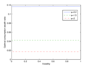
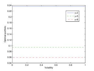
Figure 1. Both figures use parameters in (3.3), and $r=0.05$, $\delta=0.08$, $\ell=0.0225$. They are both time $0$ values for a problem with time horizon $T=10$ years. The left panel takes $\gamma=5$, and the right panel uses $\psi=1.5$.

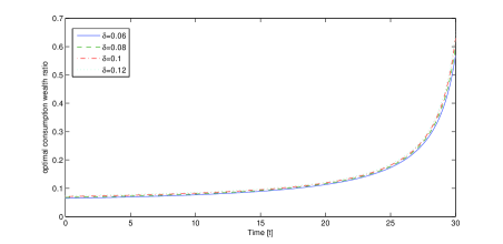
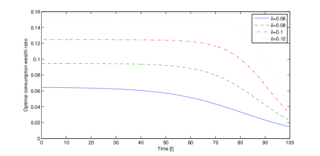
Figure 2. Optimal consumption wealth ratio as a function of time when volatility is $20\%$. Both figures use parameters in (3.3), $r=0.05$, $\ell=0.0225$, and $\gamma=5$. The upper panel takes $\psi=0.2$ and $T=30$ years. The lower panel fixes $\psi=1.5$ and $T=100$ years.

3.2. Linear diffusion

Both the interest rate and the excess return of risky assets in the following model are linear functions of a state variable, which follows a $1-$dimensional Ornstein-Uhlenbeck process. This model has been studied in [24] and [43] for the time separable utility setting, and in [7] for recursive utilities in a discrete time setting. The model dynamics is given by

(3.4) $$\left\{\begin{array}[]{l}dS_{t}=\text{diag}(S_{t})\left[\left(r(X_{t})1_{n}+\mu(X_{t})\right)\right]dt+\sigma dW^{\rho}_{t},\\ dX_{t}=-bX_{t}dt+adW_{t},\end{array}\right.$$

where $r(x)=r_{0}+r_{1}x$, $\mu(x)=\sigma(\lambda_{0}+\lambda_{1}x)$, with $r_{0},r_{1}\in\mathbb{R},\lambda_{0},\lambda_{1}\in\mathbb{R}^{n},\sigma\in\mathbb{R}^{n\times n},b,a\in\mathbb{R}$, and $\rho\in\mathbb{R}^{n}$. These coefficients satisfy

Assumption 3.3.

$a,b>0$, either $r_{1}=0$ or $\lambda_{1}^{\prime}\sigma^{\prime}\Sigma^{-1}\sigma\lambda_{1}>0$.

This assumption implies that Assumption 2.6 is satisfied with $E=\mathbb{R}$. Under following parameter restrictions, statements of Theorems 2.14 and 2.16 hold.

Proposition 3.4.

When $\gamma,\psi>1$, let Assumption 3.3 and the following parameter restrictions hold:

1. Either $-b+\frac{1-\gamma}{\gamma}a\lambda^{\prime}_{1}\sigma^{\prime}\Sigma^{-1}\sigma\rho<0$ or $\lambda_{1}^{\prime}\sigma^{\prime}\Sigma^{-1}\sigma\lambda_{1}>0$;

2. $(\psi-1)\left[\frac{b\lambda^{\prime}_{1}\rho}{a}+\frac{1}{2}\lambda^{\prime}_{1}(\psi 1_{n\times n}-(\psi-1)\rho\rho^{\prime})\lambda_{1}\right]<\frac{b^{2}}{2a^{2}}$.

Then statements of Theorems 2.14 and 2.16 hold.

In the above item i), observe that $(-b+\frac{1-\gamma}{\gamma}a\lambda^{\prime}_{1}\sigma^{\prime}\Sigma^{-1}\sigma\rho)X$ is the drift of $X$ under $\overline{\mathbb{P}}$. Therefore item i) assumes that either $X$ is mean-reverting under $\overline{\mathbb{P}}$ or the excess rate of return has a linear growth component of the state variable. Item ii) is interpreted similarly as Proposition 3.2 ii) . In particular, when $\psi>1$, the inequality in item ii) is satisfied when

(3.5) $$b\lambda^{\prime}_{1}\rho\leq-\frac{1}{2}\psi a\lambda^{\prime}_{1}\lambda_{1}.$$

This condition already covers many empirically relevant specifications. For example, in [3] and [43], a single risky asset was considered and parameter values (in monthly units) are:

(3.6) $$\lambda_{1}=1,\quad\sigma=0.0436,\quad b=0.0226,\quad a=0.0189,\quad\rho=-0.935,\quad\text{ and }\quad\psi=1.5.$$

Figure 3 demonstrates the optimal consumption wealth ratio $c^{*}/\mathcal{W}^{\pi^{*}}$ and optimal investment fraction $\pi^{*}$ with respect to the state variable $X$.

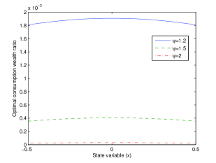
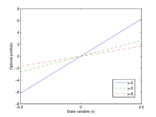
Figure 3. Both figures use parameters in (3.6), and $r=0.0014$, and $\delta=0.0052$. They are both time $0$ values for a problem with time horizon $T=12$ months. The left panel takes $\gamma=5$. The optimal consumption wealth ratio for the $\psi=0.2$ case is much larger than those displaced in the left panel. The right panel takes $\psi=1.5$.

Appendix A Proofs in Section 2.1

Let us first introduce several notation which will used throughout the appendices.

• Let $\mathcal{S}^{2}$ denote the space of all $1-$dimensional continuous adapted processes $(Y_{t})_{0\leq t\leq T}$ such that the norm $\mathbb{E}\left[\sup_{0\leq s\leq T}|Y_{s}|^{2}\right]<\infty$.

• Let $\mathcal{S}^{\infty}$ be the subspace of $\mathcal{S}^{2}$ such that the norm $\left\|\sup_{0\leq s\leq T}|Y_{s}|\right\|_{\infty}<\infty$.

• Denote by $\mathcal{T}$ the set of all $\mathcal{F}-$stopping time $\tau$ such that $0\leq\tau\leq T$. The process $Y$ is of class $D$ if the family $\{Y_{\tau};\tau\in\mathcal{T}\}$ is uniformly integrable.

• Let $\mathcal{M}^{2}$ denote the class of (multidimensional) predictable processes $(Z_{t})_{0\leq t\leq T}$ such that $\mathbb{E}\left[\int_{0}^{T}|Z_{s}|^{2}ds\right]<\infty$.

• Denote by BMO the class of martingales $M$ such that $\sup_{\tau\in\mathcal{T}}\left\|\mathbb{E}[|\langle M\rangle_{T}-\langle M\rangle_{\tau}|\,|\,\mathcal{F}_{\tau}]\right\|_{\infty}<\infty$.

Proof of Proposition 2.2.

The proof is split into several steps. First when the terminal condition is bounded, the solution is constructed by slightly modifying the proof of [34, Theorem 2.2]. For general terminal conditions, the solution is obtained by the localization technique in [6]. Finally, uniqueness is proved and (2.2) is verified. For simplicity of notation, we denote $\xi=e^{-\delta\theta T}c_{T}^{1-\gamma}$ throughout this proof.

Step 1: Bounded terminal condition. When $\xi^{2}\leq C$ for some constant $C$, consider the following truncated BSDE:

(A.1) $$Y^{n}_{t}=\xi+\int_{t}^{T}F^{n}(s,c_{s},Y^{n}_{s})\,ds-\int_{t}^{T}Z^{n}_{s}dB_{s},$$

where $F^{n}(t,c_{t},y)=\delta\theta e^{-\delta t}(c_{t}^{1-\frac{1}{\psi}}\wedge n)(|y|\wedge n)^{1-\frac{1}{\theta}}$. Note that $y\mapsto F^{n}(t,c_{t},y)$ is Lipschitz, in particular, it is differentiable at $y=0$ due to $1-1/\theta>0$. Therefore (A.1) admits a unique solution $(Y^{n},Z^{n})\in\mathcal{S}^{2}\times\mathcal{M}^{2}$. The first component of such solution is also nonnegative. Indeed, consider (A.1) with zero as the terminal condition. Such BSDE admits a unique solution $(\tilde{Y}^{n},\tilde{Z}^{n})\equiv(0,0)$ in $\mathcal{S}^{2}\times\mathcal{M}^{2}$. Since $\xi\geq 0$, it follows from the comparison theorem for BSDEs with Lipschitz generators that $Y^{n}\geq\tilde{Y}^{n}=0$. On the other hand, since $\theta<0$, $F^{n}$ is decreasing in $n$, the comparison theorem then implies that $(Y^{n})_{n}$ is decreasing. Hence $Y:=\downarrow\lim_{n\rightarrow\infty}Y^{n}$ is well defined and nonnegative.

To take the limit of $(Y^{n},Z^{n})_{n}$, let us derive the following uniform estimate. Applying Itô’s formula to $(Y^{n})^{2}$ yields

$$(Y^{n})_{t}^{2}+\mathbb{E}_{t}\left[\int_{t}^{T}|Z^{n}_{s}|^{2}\,ds\right]=\mathbb{E}_{t}\left[\xi^{2}\right]+2\,\mathbb{E}_{t}\left[\int_{t}^{T}Y^{n}_{s}F^{n}(s,c_{s},Y^{n}_{s})\,ds\right]\leq\mathbb{E}_{t}[\xi^{2}]\leq C,\quad\text{for any }t,n,$$

where the first inequality follows from $Y^{n}\geq 0$ and $F^{n}\leq 0$. The previous estimate yields

(A.2) $$(Y^{n})^{2}\leq C\quad\text{and}\quad\mathbb{E}\left[\int_{0}^{T}|Z^{n}_{s}|^{2}\,ds\right]\leq C,\quad\text{ for any }n.$$

Therefore there exists $Z\in\mathcal{M}^{2}$ such that $(Z^{n})_{n}$ converges to $Z$ weakly. Note that $\lim_{n\rightarrow\infty}F^{n}(t,c_{t},y)=F(t,c_{t},y)$, $\lim_{n\rightarrow\infty}Y^{n}=Y$, and

$$0\geq F^{n}(t,c_{t},Y^{n}_{t})\geq F(t,c_{t},Y^{n}_{t})\geq C^{\frac{1}{2}-\frac{1}{2\theta}}\delta\theta e^{-\delta t}c_{t}^{1-\frac{1}{\psi}},\quad\text{ for any }n,$$

where the third inequality holds due to the first estimate in (A.2). The dominated convergence theorem then implies that

$$\lim_{n\rightarrow\infty}\int_{t}^{T}\left|F^{n}(s,c_{s},Y^{n}_{s})-F(s,c_{s},Y_{s})\right|ds=0,\quad\text{ for any }t.$$

Now we prove the convergence of $(Z^{n})_{n}$ in $\mathcal{M}^{2}$. Applying Itô’s formula to $|Y^{n}-Y^{m}|^{2}$ yields

(A.3) $$\begin{split}&\mathbb{E}[|Y^{n}_{0}-Y^{m}_{0}|^{2}]+\mathbb{E}\left[\int_{0}^{T}|Z^{n}_{s}-Z^{m}_{s}|^{2}\,ds\right]\\ =&2\,\mathbb{E}\left[\int_{0}^{T}\left(Y^{n}_{s}-Y^{m}_{s}\right)\left(F^{n}(Y^{n}_{s})-F^{m}(Y^{m}_{s})\right)\,ds\right]\\ =&2\,\mathbb{E}\left[\int_{0}^{T}\left(Y^{n}_{s}-Y^{m}_{s}\right)\left(F^{n}(Y^{n}_{s})-F^{n}(Y^{m}_{s})\right)\,ds\right]+2\,\mathbb{E}\left[\int_{0}^{T}\left(Y^{n}_{s}-Y^{m}_{s}\right)\left(F^{n}(Y^{m}_{s})-F^{m}(Y^{m}_{s})\right)\,ds\right]\\ \leq&2\,\mathbb{E}\left[\int_{0}^{T}\left(Y^{n}_{s}-Y^{m}_{s}\right)\left(F^{n}(Y^{m}_{s})-F^{m}(Y^{m}_{s})\right)\,ds\right]\\ \leq&4\delta|\theta|C^{\frac{1}{2}-\frac{1}{2\theta}}\,\mathbb{E}\left[\int_{0}^{T}e^{-\delta s}\left|c_{s}^{1-\frac{1}{\psi}}\wedge n-c_{s}^{1-\frac{1}{\psi}}\wedge m\right|\,ds\right],\end{split}$$

where the first inequality holds due to the fact that $y\mapsto F^{n}(t,c_{t},y)$ is decreasing and the second inequality follows from the first estimate in (A.2). Since $c\in\mathcal{C}_{a}$, the dominated convergence theorem implies the right hand side of (A.3) converges to zero as $n,m\rightarrow\infty$. Combining the previous convergence with the weak convergence of $(Z^{n})_{n}$, we obtain

$$\lim_{n\rightarrow\infty}\mathbb{E}\left[\int_{0}^{T}|Z^{n}_{s}-Z_{s}|^{2}\,ds\right]=0,$$

The Burkholder-Davis-Gundy inequality then implies

$$\mathbb{P}-\lim_{n\rightarrow\infty}\sup_{t\leq T}\left|\int_{t}^{T}(Z^{n}_{s}-Z_{s})dB_{s}\right|=0,$$

where $\mathbb{P}-\lim$ stands for the convergence in probability. Passing to a subsequence, we obtain almost sure convergence. Therefore, sending $n\rightarrow\infty$ in (A.1), we obtain that $(Y,Z)\in\mathcal{S}^{\infty}\times\mathcal{M}^{2}$ solves (2.4) and $Y$ is nonnegative. Moreover, since

$$|Y^{n}_{t}-Y^{m}_{t}|\leq\int_{t}^{T}\left|F^{n}(s,c_{s},Y^{n}_{s})-F^{m}(s,c_{s},Y^{m}_{s})\right|ds+\left|\int_{t}^{T}(Z^{n}_{s}-Z^{m}_{s})dB_{s}\right|,$$

after taking limits on $m$ and supremum over $t$, we obtain

$$\sup_{t\leq T}|Y^{n}_{t}-Y_{t}|\leq\int_{0}^{T}\left|F^{n}(s,c_{s},Y^{n}_{s})-F(s,c_{s},Y_{s})\right|ds+\sup_{t\leq T}\left|\int_{t}^{T}(Z^{n}_{s}-Z_{s})dB_{s}\right|.$$

Therefore $(Y^{n})_{n}$ converges to $Y$ uniformly in $t$, implying that $Y$ is a continuous process.

Step 2: General terminal condition. When $\xi$ is not bounded, set $\xi^{n}:=\xi\wedge n$ and consider

$$Y^{n}_{t}=\xi^{n}+\int_{t}^{T}F(s,c_{s},Y^{n}_{s})\,ds-\int_{t}^{T}Z^{n}_{s}\,dB_{s}.$$

Results from the previous step imply that this BSDE admits a solution $(Y^{n},Z^{n})\in\mathcal{S}^{\infty}\times\mathcal{M}^{2}$ with $Y^{n}\geq 0$. Moreover, since $F\leq 0$, $Y^{n}_{t}\leq\mathbb{E}_{t}[\xi]$ for all $n$ and $t\in[0,T]$. This a priori bound allows us to construct a solution to (2.4) via the localization technique in [6]. We outline the construction below.

Consider $\tau_{k}:=\inf\{t\geq 0\,:\,\mathbb{E}_{t}[\xi]\geq k\}\wedge T$ for each $k\in\mathbb{N}$. Then $(Y^{n,k}_{t},Z^{n,k}_{t}):=(Y^{n}_{t\wedge\tau_{k}},Z^{n}_{t}\mathbb{I}_{\{t\leq\tau_{k}\}})$ satisfies the following BSDE

$$Y^{n,k}_{t}=Y^{n}_{\tau_{k}}+\int_{t}^{T}\mathbb{I}_{\{s\leq\tau_{k}\}}F(s,c_{s},Y^{n,k}_{s})\,ds-\int_{t}^{T}Z^{n,k}_{s}dB_{s}.$$

Since $0\leq Y^{n,k}_{s}\leq\mathbb{E}_{s\wedge\tau_{k}}[\xi]\leq k$, we have

$$0\geq F(s,c_{s},Y^{n,k}_{s})\geq\delta\theta k^{1-\frac{1}{\theta}}e^{-\delta s}c_{s}^{1-\frac{1}{\psi}}.$$

Then $c\in\mathcal{C}_{a}$ implies $\mathbb{E}[\int_{0}^{T}F(s,c_{s},Y^{n,k}_{s})ds]<\infty$. On the other hand, since $\xi^{n}\leq\xi^{n+1}$ and $y\mapsto F(\cdot,\cdot,y)$ satisfies the monotonicity condition, then the comparison result (cf. [34, Theorem 2.4]) implies $Y^{n,k}\leq Y^{n+1,k}$. Utilizing the same argument as in Step 1, we obtain $\tilde{Y}^{k}:=\uparrow\lim_{n}Y^{n,k}$ and $\tilde{Z}^{k}\in\mathcal{M}^{2}$ such that $\lim_{n}Z^{n,k}=\tilde{Z}^{k}$ in $\mathcal{M}^{2}$, and $(\tilde{Y}^{k},\tilde{Z}^{k})$ solves the BSDE

(A.4) $$\tilde{Y}^{k}_{t}=\tilde{Y}^{k}_{\tau_{k}}+\int_{t}^{T}\mathbb{I}_{\{s\leq\tau_{k}\}}F(s,c_{s},\tilde{Y}^{k}_{s})\,ds-\int_{t}^{T}\tilde{Z}^{k}_{s}dB_{s},$$

where $\tilde{Y}^{k}_{\tau_{k}}=\uparrow\lim_{n}Y^{n}_{\tau_{k}}$. Following from the definition of $(\tilde{Y}^{k},\tilde{Z}^{k})$, $\tilde{Y}^{k+1}_{t\wedge\tau_{k}}=\tilde{Y}^{k}_{t}$ and $\tilde{Z}^{k+1}_{t}\mathbb{I}_{\{t\leq\tau_{k}\}}=\tilde{Z}^{k}_{t}$. Therefore we define

$$Y_{t}:=\tilde{Y}^{k}_{t}\quad\text{and}\quad Z_{t}:=\tilde{Z}^{k}_{t},\quad\text{when }t\in[0,\tau_{k}].$$

This construction implies $\lim_{t\rightarrow T}Y_{t}=\xi$. Indeed, on $\{\xi\leq k\}$, $\tau_{k}=T$ and $\lim_{t\rightarrow T}Y^{n}_{t}=\xi$ for any $n\geq k$. Therefore $\lim_{t\rightarrow T}Y_{t}=\lim_{t\rightarrow\tau_{k}}\tilde{Y}^{k}_{t}=\lim_{t\rightarrow\tau_{k}}Y^{n,k}_{t}=\lim_{t\rightarrow T}Y^{n}_{t}=\xi$ on $\{\xi\leq k\}$ when $n\geq k$. This implies $\lim_{t\rightarrow T}Y_{t}=\xi$, since $\uparrow\lim_{k\rightarrow\infty}\{\xi\leq k\}=\Omega$. Now sending $k\rightarrow\infty$ on both sides of (A.4), we confirm that $(Y,Z)$ solves (2.4). By this construction, $Y$ is continuous and satisfies $0\leq Y_{t}\leq\mathbb{E}_{t}[\xi]$ for $t\in[0,T]$, hence $Y$ is of class $D$. The same argument as in [6, Page 612] shows $\int_{0}^{T}|Z_{t}|^{2}dt<\infty$.

Step 3: Remaining statements. For future reference, we prove a comparison result for (2.4). Let $(Y,Z)$ (resp. $(\tilde{Y},\tilde{Z})$) be a super-solution (resp. sub-solution) to (2.4), i.e.,

$$Y+\int_{0}^{\cdot}F(s,c_{s},Y_{s})ds\text{ is a local supermartingale and }\tilde{Y}+\int_{0}^{\cdot}F(s,c_{s},\tilde{Y}_{s})ds\text{ is a local submartingale},$$

with $Y_{T}\geq\xi\geq\tilde{Y}_{T}$, meanwhile $Z$ and $\tilde{Z}$ are determined by Doob-Meyer decomposition and martingale representation. Assuming that both $Y$ and $\tilde{Y}$ are of class $D$, then $Y\geq\tilde{Y}$. Moreover, if $Y_{T}>\tilde{Y}_{T}$, then $Y_{t}>\tilde{Y}_{t}$ for any $t\leq T$.

To prove this comparison result, define

$$\alpha_{t}:=\left\{\begin{array}[]{ll}\frac{F(t,c_{t},Y_{t})-F(t,c_{t},\tilde{Y}_{t})}{Y_{t}-\tilde{Y}_{t}},&Y_{t}\neq\tilde{Y}_{t}\\ 0,&Y_{t}=\tilde{Y}_{t}\end{array}\right..$$

Since $y\mapsto F(\cdot,\cdot,y)$ is decreasing, we have $\alpha\leq 0$. It then follows that $e^{\int_{0}^{\cdot}\alpha_{s}ds}(Y-\tilde{Y})$ is a local supermartingale, hence a supermartingale, since the exponential factor is bounded and both $Y$ and $\tilde{Y}$ are of class $D$. Therefore, $Y_{T}\geq\tilde{Y}_{T}$ implies $Y\geq\tilde{Y}$. Moreover when $Y_{T}>\tilde{Y}_{T}$, we obtain the strict comparison $Y_{t}>\tilde{Y}_{t}$ for any $t\leq T$. The uniqueness follows from the comparison result directly. Since $\gamma>1$, then $\xi=e^{-\delta\theta T}c_{T}^{1-\gamma}>0$. Therefore $Y>0$ follows from the strict comparison.

Finally, we verify that $V^{c}$ satisfies (2.2). To this end, since $(Y,Z)$ solves (2.4), $(V^{c}_{t},Z^{c}_{t})=e^{\delta\theta t}(Y_{t},Z_{t})/(1-\gamma)$ satisfies (2.3), implying that $V^{c}+\int_{0}^{\cdot}f(c_{s},V^{c}_{s})ds$ is a local martingale. Taking a localizing sequence $(\sigma_{n})_{n\geq 1}$ for $V^{c}+\int_{0}^{\cdot}f(c_{s},V^{c}_{s})ds$, we obtain

$$V^{c}_{0}+\delta\theta\mathbb{E}\left[\int_{0}^{T\wedge\sigma_{n}}V^{c}_{s}ds\right]=\mathbb{E}\left[V^{c}_{T\wedge\sigma_{n}}+\int_{0}^{T\wedge\sigma_{n}}\delta\frac{c_{s}^{1-\frac{1}{\psi}}}{1-\frac{1}{\psi}}\left((1-\gamma)V^{c}_{s}\right)^{1-\frac{1}{\theta}}ds\right].$$

Sending $n\rightarrow\infty$ on both sides, note that $V^{c}\leq 0$ and $\psi>1$, therefore the integrand on the left side is negative and the integrand on the right side is positive. The monotone convergence theorem and the class $D$ property of $V^{c}$ then yield

(A.5) $$V^{c}_{0}+\delta\theta\mathbb{E}\left[\int_{0}^{T}V^{c}_{s}ds\right]=\mathbb{E}\left[U(c_{T})+\int_{0}^{T}\delta\frac{c_{s}^{1-\frac{1}{\psi}}}{1-\frac{1}{\psi}}\left((1-\gamma)V^{c}_{s}\right)^{1-\frac{1}{\theta}}ds\right].$$

Since $0\geq\mathbb{E}\left[\int_{0}^{T}V^{c}_{s}ds\right]=\frac{1}{1-\gamma}\mathbb{E}\left[\int_{0}^{T}e^{\delta\theta s}Y_{s}ds\right]\geq\frac{1}{1-\gamma}\mathbb{E}\left[\int_{0}^{T}Y_{s}ds\right]\geq\frac{1}{1-\gamma}\int_{0}^{T}\mathbb{E}[\xi]ds>-\infty$, where the second inequality holds since $\gamma>1$ and $\theta<0$, the third inequality follows from $Y_{s}\leq\mathbb{E}_{s}[\xi]$ and $\gamma>1$. Subtracting $\delta\theta\mathbb{E}\left[\int_{0}^{T}V^{c}_{s}ds\right]$ on both sides of (A.5), we confirm (2.2). ∎

The concavity of $c\mapsto V^{c}$ is proved in the following. This proof utilizes simultaneously the joint concavity of the generator for (2.5) and the class $D$ property of the solution to (2.4).

Proof of Proposition 2.4.

Denote the generator of (2.5) as $\mathbb{F}(t,c_{t},y,z)=\delta e^{-\delta t}\frac{c_{t}^{1-\frac{1}{\psi}}}{1-\frac{1}{\psi}}+\frac{1}{2}(\theta-1)\frac{z^{2}}{y}$. For $c,\tilde{c}$ and $\alpha c+(1-\alpha)\tilde{c}\in\mathcal{C}_{a}$, denote $\Delta X=\alpha X+(1-\alpha)\tilde{X}$, for $X=c,\mathbb{Y},\mathbb{Z}$ and $\tilde{X}=\tilde{c},\tilde{\mathbb{Y}},\tilde{\mathbb{Z}}$, respectively. It follows from (2.5) that

$$d\Delta\mathbb{Y}_{t}=\left[-\delta e^{-\delta t}\frac{\Delta c_{t}^{1-\frac{1}{\psi}}}{1-\frac{1}{\psi}}-\frac{1}{2}(\theta-1)\frac{\Delta\mathbb{Z}_{t}^{2}}{\Delta\mathbb{Y}_{t}}+A_{t}\right]dt+\Delta\mathbb{Z}_{t}dB_{t},$$

where, due to the concavity of $(c_{t},y,z)\mapsto\mathbb{F}(t,c_{t},y,z)$,

$$A_{t}=\frac{\delta e^{-\delta t}}{1-\frac{1}{\psi}}\left[\Delta c_{t}^{1-\frac{1}{\psi}}-\alpha c_{t}^{1-\frac{1}{\psi}}-(1-\alpha)\tilde{c}_{t}^{1-\frac{1}{\psi}}\right]+\frac{1}{2}(\theta-1)\left[\frac{\Delta\mathbb{Z}^{2}_{t}}{\Delta\mathbb{Y}_{t}}-\alpha\frac{\mathbb{Z}^{2}_{t}}{\mathbb{Y}_{t}}-(1-\alpha)\frac{\tilde{\mathbb{Z}}_{t}^{2}}{\tilde{\mathbb{Y}}_{t}}\right]\geq 0,$$

and $\Delta\mathbb{Y}_{T}\leq e^{-\delta T}\Delta c_{T}^{1-1/\psi}/(1-1/\psi)$. Set

$$\Delta Y=((1-1/\psi)\Delta\mathbb{Y})^{\theta}\quad\text{ and }\quad\Delta Z=(1-\gamma)((1-1/\psi)\Delta\mathbb{Y})^{\theta-1}\Delta\mathbb{Z}.$$

Itô’s formula yields

$$d\Delta Y_{t}=(-\delta\theta e^{-\delta t}\Delta c_{t}^{1-\frac{1}{\psi}}\Delta Y_{t}^{1-\frac{1}{\theta}}+(1-\gamma)\Delta Y_{t}^{1-\frac{1}{\theta}}A_{t})\,dt+\Delta Z_{t}dB_{t},$$

where $(1-\gamma)\Delta Y_{t}^{1-1/\theta}A_{t}\leq 0$. On the other hand, $\Delta Y_{T}\geq e^{-\delta\theta T}\Delta c_{T}^{1-\gamma}$. Therefore $(\Delta Y,\Delta Z)$ is a super-solution to (2.4). On the other hand, $\Delta Y$ is of class $D$. Indeed, since $\theta<0$,

(A.6) $$\Delta Y=\left(\left(1-1/\psi\right)\Delta\mathbb{Y}\right)^{\theta}\leq\alpha\left(\left(1-1/\psi\right)\mathbb{Y}\right)^{\theta}+(1-\alpha)(\left(1-1/\psi\right)\tilde{\mathbb{Y}})^{\theta}=\alpha Y+(1-\alpha)\tilde{Y},$$

where $Y$ (resp. $\tilde{Y}$) is the first component of the solution to (2.4) with $c$ (resp. $\tilde{c}$). Therefore, $\Delta Y$ is of class $D$, because both $Y$ and $\tilde{Y}$ are. Now consider $Y^{\Delta c}$ as the first component of solution of (2.4) where $c$ is replaced by $\Delta c$. It then follows from (A.6) and the comparison result in Step 3 of the previous proof that

$$\alpha Y_{0}+(1-\alpha)\tilde{Y}_{0}\geq\Delta Y_{0}\geq Y_{0}^{\Delta c}.$$

Dividing the previous inequality by $(1-\gamma)$ on both sides, we confirm $\alpha V^{c}_{0}+(1-\alpha)V^{\tilde{c}}_{0}\leq V^{\alpha c+(1-\alpha)\tilde{c}}_{0}$. ∎

Appendix B Proofs in Section 2.2

Even though the generator $H$ in (2.12) has an exponential term in $y$, the parameter specification $\gamma>1$ and $\psi>1$ allow us to derive a priori bounds for $Y$. Then a solution to (2.12) is constructed via the localization technique in [6].

Proof of Proposition 2.9.

Due to Assumption 2.7 i), $\overline{W}:=W-\int_{0}^{\cdot}\frac{1-\gamma}{\gamma}\rho^{\prime}\sigma^{\prime}\Sigma^{-1}\mu(X_{s})ds$ is a $\overline{\mathbb{P}}-$Brownian motion. Therefore, (2.12) can be rewritten under $\overline{\mathbb{P}}$, and all expectations are taken with respect to $\overline{\mathbb{P}}$ throughout this proof. On the other hand, recall that $\gamma>1$ and $r+\frac{1}{2\gamma}\mu^{\prime}\Sigma^{-1}\mu$ is bounded from below. Therefore there exists a constant $h_{max}$ such that $h\leq h_{max}$. However, $\mu^{\prime}\Sigma^{-1}\mu$, in many widely used models, is an unbounded function of the state variable, hence $h$ and $H(t,0,0)=h_{t}-\delta\theta+\theta\frac{\delta^{\psi}}{\psi}$ are not bounded from below. Therefore we introduce

(B.1) $$\mathcal{Y}_{t}=\xi+\int_{t}^{T}\mathcal{H}(s,\mathcal{Y}_{s},Z_{s})ds-\int_{t}^{T}Z_{s}d\overline{W}_{s},$$

where $\mathcal{Y}_{t}=Y_{t}+\int_{0}^{t}(h_{s}-\delta\theta)\,ds$, $\xi=\int_{0}^{T}(h_{s}-\delta\theta)\,ds$, and

$$\mathcal{H}(t,y,z)=\frac{1}{2}zM_{t}z^{\prime}+\theta\frac{\delta^{\psi}}{\psi}e^{\frac{\psi}{\theta}\int_{0}^{t}h_{s}-\delta\theta\,ds}e^{-\frac{\psi}{\theta}y}.$$

Consider a truncated version of (B.1):

(B.2) $$\mathcal{Y}^{n}_{t}=\xi^{n}+\int_{t}^{T}\mathcal{H}^{n}(s,\mathcal{Y}^{n}_{s},Z^{n}_{s})\,ds-\int_{t}^{T}Z^{n}_{s}d\overline{W}_{s},$$

where $\xi^{n}=\int_{0}^{T}h_{s}\vee(-n)-\delta\theta\,ds$ is bounded and

$$\mathcal{H}^{n}(t,y,z)=\frac{1}{2}zM_{t}z^{\prime}+\theta\frac{\delta^{\psi}}{\psi}e^{\frac{\psi}{\theta}\int_{0}^{t}h_{s}\vee(-n)-\delta\theta\,ds}\left(e^{-\frac{\psi}{\theta}y}\wedge n\right).$$

This truncated generator $\mathcal{H}^{n}$ is Lipschitz in $y$ and quadratic in $z$. Indeed, since eigenvalues of $\sigma^{\prime}\Sigma^{-1}\sigma$ is either $0$ or $1$, $0\leq z\rho^{\prime}\sigma^{\prime}\Sigma^{-1}\sigma\rho z^{\prime}\leq z\rho^{\prime}\rho z^{\prime}\leq|z|^{2}$. Then $\gamma>1$ and the definition of $M$ after (2.13) implies

(B.3) $$0<\frac{1}{\gamma}|z|^{2}\leq zM(X)z^{\prime}\leq|z|^{2}.$$

Therefore it follows from [25, Theorem 2.3] that (B.2) admits a solution $(\mathcal{Y}^{n},Z^{n})\in\mathcal{S}^{\infty}\times\mathcal{M}^{2}$. Moreover, due to $\theta<0$, $\mathcal{H}^{n}$ is decreasing in $n$. The construction of $\mathcal{Y}^{n}$ in [25, Theorem 2.3] yields $\mathcal{Y}^{n}\geq\mathcal{Y}^{n+1}$. In what follows, we derive a priori bounds on $\mathcal{Y}^{n}$ uniformly in $n$. This uniform estimate facilitates the construction of a solution to (B.1).

On the one hand, $\theta<0$ and the third inequality in (B.3) yield $\mathcal{H}^{n}(t,y,z)\leq\frac{1}{2}|z|^{2}$. Consider

$$\overline{Y}^{n}_{t}=\xi^{n}+\int_{t}^{T}\frac{1}{2}|\overline{Z}^{n}_{s}|^{2}ds-\int_{t}^{T}\overline{Z}^{n}_{s}\,d\overline{W}_{s},$$

which has an explicit solution $\overline{Y}^{n}_{t}=\log\mathbb{E}_{t}\left[e^{\int_{0}^{T}h_{s}\vee(-n)-\delta\theta\,ds}\right]$. Then

(B.4) $$\overline{Y}^{n}_{t}-\int_{0}^{t}h_{s}\vee(-n)-\delta\theta\,ds=\log\mathbb{E}_{t}\left[e^{\int_{t}^{T}h_{s}\vee(-n)-\delta\theta\,ds}\right]\leq(h_{max}-\delta\theta)(T-t).$$

On the other hand, when $y-\int_{0}^{t}h_{s}\vee(-n)-\delta\theta\,ds\leq(h_{max}-\delta\theta)(T-t)$, the first inequality in (B.3) and $\theta<0$ imply $\mathcal{H}^{n}(t,y,z)\geq\theta\frac{\delta^{\psi}}{\psi}e^{(\delta\psi-\frac{\psi}{\theta}h_{max})T}$. Therefore consider the BSDE

$$\underline{Y}_{t}=\xi+\theta\frac{\delta^{\psi}}{\psi}e^{(\delta\psi-\frac{\psi}{\theta}h_{max})T}(T-t)-\int_{t}^{T}\underline{Z}_{s}d\overline{W}_{s},$$

whose solution $\underline{Y}$ admits a representation $\underline{Y}_{t}=\mathbb{E}_{t}[\xi]+\theta\frac{\delta^{\psi}}{\psi}e^{(\delta\psi-\frac{\psi}{\theta}h_{max})T}(T-t)$.

Now since $\mathcal{H}^{n}$ is sandwiched between two generators with simpler forms, comparison result yields

(B.5) $$\mathbb{E}_{t}[\xi]+\theta\frac{\delta^{\psi}}{\psi}e^{(\delta\psi-\frac{\psi}{\theta}h_{max})T}(T-t)=\underline{Y}_{t}\leq\mathcal{Y}^{n}_{t}\leq\overline{Y}^{n}_{t}=\log\mathbb{E}_{t}\left[e^{\int_{0}^{T}h_{s}\vee(-n)-\delta\theta\,ds}\right]\leq(h_{max}-\delta\theta)T,$$

for any $n>0$. These uniform bounds on $\mathcal{Y}^{n}$ allow us to construct a solution $(\mathcal{Y},Z)$ to (B.1) using the localization technique in [6, Theorem 2]; see also Step 2 in the proof of Proposition 2.2. The resulting $\mathcal{Y}$ satisfies

(B.6) $$\mathbb{E}_{t}[\xi]+\theta\frac{\delta^{\psi}}{\psi}e^{(\delta\psi-\frac{\psi}{\theta}h_{max})T}(T-t)\leq\mathcal{Y}_{t}\leq\log\mathbb{E}_{t}\left[e^{\xi}\right].$$

The previous inequalities imply that $\lim_{t\rightarrow T}\mathcal{Y}_{t}=\xi$. Hence $\mathcal{Y}$ satisfies the terminal condition of (B.1). The desired estimates on $Y$ follows after subtracting $\int_{0}^{t}h_{s}-\delta\theta\,ds$ on both sides of the previous inequalities, in particular,

(B.7) $$Y_{t}=\mathcal{Y}_{t}-\int_{0}^{t}h_{s}-\delta\theta\,ds\leq\log\mathbb{E}_{t}\left[e^{\int_{t}^{T}(h_{s}-\delta\theta)ds}\right]\leq(h_{max}-\delta\theta)(T-t).$$

For the statement on $Z$, take a localization sequence $(\sigma_{n})_{n}$ for $\int_{0}^{\cdot}Z_{s}d\overline{W}_{s}$, (B.1) yields

$$\frac{1}{2}\mathbb{E}\left[\int_{0}^{\sigma_{n}}Z_{s}M_{s}Z_{s}^{\prime}ds\right]=\mathcal{Y}_{0}-\mathbb{E}[\mathcal{Y}_{\sigma_{n}}]-\theta\frac{\delta^{\psi}}{\psi}\mathbb{E}\left[\int_{0}^{\sigma_{n}}e^{\frac{\psi}{\theta}\int_{0}^{s}h_{u}-\delta\theta du}e^{-\frac{\psi}{\theta}\mathcal{Y}_{s}}ds\right].$$

Sending $n\rightarrow\infty$ on both sides, applying the second inequality in (B.3) to the left-hand side, the first inequality in (B.6) to the second term on the right-hand side, and (B.7) to the third term, we confirm $\mathbb{E}[\int_{0}^{T}|Z_{s}|^{2}ds]<\infty$. ∎

The following several results prepare the proofs of Theorems 2.14 and 2.16. First we show $\frac{w^{1-\gamma}}{1-\gamma}e^{Y_{0}}$ is an upper bound for the optimal value among permissible strategies.

Lemma B.1.

Let Assumption 2.7 hold. For any permissible $(\pi,c)$,

(B.8) $$\frac{w^{1-\gamma}}{1-\gamma}e^{Y_{0}}\geq V^{c}_{0},$$

where $V^{c}$ is defined in Proposition 2.2, $Y$ is constructed in Proposition 2.9, and $c$ is financed by $\pi$ via (2.8).

Proof.

This proof extends the technique in [20] to recursive utilities. For a permissible $(\pi,c)$, define

$$R^{\pi,c}_{t}:=\frac{(\mathcal{W}_{t})^{1-\gamma}}{1-\gamma}e^{Y_{t}}+\int_{0}^{t}f\left(c_{s},\frac{(\mathcal{W}_{s})^{1-\gamma}}{1-\gamma}e^{Y_{s}}\right)\,ds,\quad t\in[0,T],$$

where $\mathcal{W}=\mathcal{W}^{\pi,c}$. Then (2.11) and (2.13) imply that $R$ is a local supermartingale. Due to Doob-Meyer decomposition and martingale representation, there exist an increasing process $A$ and $Z^{R}$ such that $R^{\pi,c}=-A+\int_{0}^{\cdot}Z^{R}_{s}dB_{s}$. Therefore, $\left(\frac{(\mathcal{W})^{1-\gamma}}{1-\gamma}e^{Y},Z^{R}\right)$ is a supersolution to (2.3), whose terminal condition is $(\mathcal{W}_{T})^{1-\gamma}/(1-\gamma)\in\mathbb{L}^{1}$. Indeed, since $(\mathcal{W})^{1-\gamma}e^{Y}$ is of class $D$ by permissibility and $Y_{T}=0$, we have $\mathbb{E}[(\mathcal{W}_{T})^{1-\gamma}]<\infty$. On the other hand, consider the utility $V^{0}_{c}$ associated to the consumption stream $c$ and the terminal lump sum $\mathcal{W}_{T}$. The comparison result in the proof of Proposition 2.2 confirms (B.8). ∎

In what follows we will show that $(\pi^{*},c^{*})$ is a permissible strategy and it attains the upper bound $\frac{w^{1-\gamma}}{1-\gamma}e^{Y_{0}}$. First, we establish an important result that certain exponential local martingale associated to $\pi^{*}$ is a martingale.

Lemma B.2.

Let Assumptions 2.6, 2.7 and 2.10 hold. Then $Q:=\mathcal{E}\left(\int(1-\gamma)(\pi^{*}_{s})^{\prime}\sigma_{s}dW^{\rho}_{s}+\int Z_{s}dW_{s}\right)$ is a $\mathbb{P}-$martingale on $[0,T]$.

Proof.

It follows from (2.14), the definition of $W^{\rho}$ and $M$ that

$$(1-\gamma)(\pi^{*})^{\prime}\sigma dW^{\rho}+ZdW =\left(\frac{1-\gamma}{\gamma}\mu^{\prime}\Sigma^{-1}\sigma\rho+ZM\right)dW+\frac{1-\gamma}{\gamma}\left(\mu^{\prime}+Z\rho^{\prime}\sigma^{\prime}\right)\Sigma^{-1}\sigma\rho^{\bot}dW^{\bot}$$

$$=:L^{(1)}dW+L^{(2)}dW^{\bot}.$$

Here we suppress time subscripts to simplify notation. First we claim that if $Q^{(1)}:=\mathcal{E}(\int L^{(1)}_{s}dW_{s})$ is a martingale, so is $Q$. Indeed, for any $t\leq T$,

(B.9) $$\begin{split}\mathbb{E}[Q_{t}]&=\mathbb{E}\left[\mathcal{E}\left(\int L^{(1)}_{s}dW_{s}\right)_{t}\mathcal{E}\left(\int L^{(2)}_{s}dW^{\bot}_{s}\right)_{t}\right]\\ &=\mathbb{E}\left[\mathcal{E}\left(\int L^{(1)}_{s}dW_{s}\right)_{t}\mathbb{E}\left[\left.\mathcal{E}\left(\int L^{(2)}_{s}dW^{\bot}_{s}\right)_{t}\right|\mathcal{F}^{W}\right]\right]\\ &=\mathbb{E}\left[\mathcal{E}\left(\int L^{(1)}_{s}dW_{s}\right)_{t}\right]\\ &=1.\end{split}$$

Here $\mathcal{F}^{W}=\sigma(W_{s};0\leq s\leq T)$, the third identity follows from [21, Lemma 4.8] since $L^{(2)}$ and $W^{\bot}$ are independent, and the fourth identity is due to the martingale assumption on $Q^{(1)}$. In the remaining of the proof, we will prove the martingale property of $Q^{(1)}$.

For the sequence of subdomains $(E_{n})_{n}$ in Assumption 2.10 i), define $\tau_{n}:=\inf\{t\geq 0\,|\,X_{t}\notin E_{n}\}\wedge T$. we first prove that $Y_{\cdot\wedge\tau_{n}}$ is bounded. Since we have seen in Proposition 2.9 that $Y$ is bounded from above, it suffices to show $\mathbb{E}^{\overline{\mathbb{P}}}_{\cdot\wedge\tau_{n}}\left[\int_{\cdot\wedge\tau_{n}}^{T}h_{s}ds\right]$ is bounded from below. Then (2.15) implies that $Y_{\cdot\wedge\tau_{n}}$ is bounded as well. Due to the Markovian structure, define

$$y(t,x):=\mathbb{E}^{\overline{\mathbb{P}}}\left[\left.\int_{t}^{T}h(X_{s})\,ds\right|X_{t}=x\right].$$

The Feynman-Kac formula (see [19] when the equation is not uniformly parabolic) implies that, under Assumption 2.6, $y\in C^{1,2}([0,T]\times E)$ and it is the unique solution to

$$\partial_{t}y+\mathcal{L}y+h=0,\quad y(T,x)=0,$$

where $\mathcal{L}$ is the infinitesimal generator of $X$ under $\overline{\mathbb{P}}$. Now since $\overline{E}_{n}$ is compact, the continuity of $y$ implies that $y(\cdot\wedge\tau_{n},X_{\cdot\wedge\tau_{n}})$ is bounded.

As a solution to (2.12), $(Y,Z)$ satisfies

$$Y_{t}=Y_{\tau_{n}}+\int_{t}^{\tau_{n}}H(s,Y_{s},Z_{s})ds-\int_{t}^{\tau_{n}}Z_{s}\,dW_{s},\quad t\in[0,\tau_{n}].$$

Since both $X_{\cdot\wedge\tau_{n}}$ and $Y_{\cdot\wedge\tau_{n}}$ are bounded, it follows from the BMO-estimate for quadratic BSDEs (cf. eg. [33, Lemma 3.1]) that $\int_{0}^{\cdot\wedge\tau_{n}}Z_{s}dW_{s}$ is a BMO-martingale. Note that both $\mu^{\prime}\Sigma^{-1}\sigma\rho(X_{\cdot\wedge\tau_{n}})$ and $M(X_{\cdot\wedge\tau_{n}})$ are bounded. Therefore $\int_{0}^{\cdot\wedge\tau_{n}}L^{(1)}_{s}dW_{s}$ is a BMO-martingale as well. Then [23, Theorem 2.3] implies that $\mathcal{E}(\int L^{(1)}_{s}dW_{s})_{\cdot\wedge\tau_{n}}$ is a martingale. Therefore $d\mathbb{Q}^{n}/d\mathbb{P}:=\mathcal{E}(\int L^{(1)}_{s}dW_{s})_{\tau_{n}}$ defines $\mathbb{Q}^{n}$ on $\mathcal{F}_{\tau_{n}}$ which is equivalent to $\mathbb{P}$.

Assuming that $\lim_{n\rightarrow\infty}\mathbb{Q}^{n}(\tau_{n}<T)=0$, by the monotone convergence theorem,

$$\mathbb{E}\left[\mathcal{E}\left(\int L^{(1)}_{s}dW_{s}\right)_{T}\right] =\lim_{n\rightarrow\infty}\mathbb{E}\left[\mathcal{E}\left(\int L^{(1)}_{s}dW_{s}\right)_{\tau_{n}}\mathbb{I}_{\{\tau_{n}=T\}}\right]$$

$$=\lim_{n\rightarrow\infty}\mathbb{E}\left[\mathcal{E}\left(\int L^{(1)}_{s}dW_{s}\right)_{\tau_{n}}\right]-\lim_{n\rightarrow\infty}\mathbb{E}\left[\mathcal{E}\left(\int L^{(1)}_{s}dW_{s}\right)_{\tau_{n}}\mathbb{I}_{\{\tau_{n}<T\}}\right]$$

$$=1-\lim_{n\rightarrow\infty}\mathbb{Q}^{n}(\tau_{n}<T)$$

$$=1,$$

proving the martingale property of $\mathcal{E}(\int L^{(1)}_{s}dW_{s})$ on $[0,T]$.

It remains to prove $\lim_{n\rightarrow\infty}\mathbb{Q}^{n}(\tau_{n}<T)=0$. To this end, (2.12) yields

$$Y_{t}=Y_{0}-\int_{0}^{t}H(s,Y_{s},Z_{s})ds+\int_{0}^{t}Z_{s}dW_{s}.$$

On the other hand, recall $\mathfrak{F}$ from (2.16), we have from Itô’s formula,

$$\phi(X_{t}) =\phi(x)+\int_{0}^{t}b^{\prime}\nabla\phi(X_{s})+\frac{1}{2}\sum_{i,j=1}^{k}A_{ij}\partial^{2}_{x_{i}x_{j}}\phi(X_{s})\,ds+\int_{0}^{t}\nabla\phi^{\prime}a(X_{s})dW_{s}$$

$$=\phi(x)+\int_{0}^{t}\left[\mathfrak{F}[\phi]-\frac{1}{2}\nabla\phi^{\prime}aMa^{\prime}\nabla\phi-h-\frac{1-\gamma}{\gamma}\mu^{\prime}\Sigma^{-1}\sigma\rho a^{\prime}\nabla\phi\right]ds+\int_{0}^{t}\nabla\phi^{\prime}a(X_{s})dW_{s}$$

Taking difference of the previous two identities,

$$Y_{t}-\phi(X_{t})$$

$$=Y_{0}-\phi(x)+\int_{0}^{t}\left(Z_{s}-\nabla\phi^{\prime}a(X_{s})\right)dW_{s}$$

$$\quad-\int_{0}^{t}\left[\frac{1}{2}ZMZ^{\prime}-\frac{1}{2}\nabla\phi^{\prime}aMa^{\prime}\nabla\phi+\theta\frac{\delta^{\psi}}{\psi}e^{-\frac{\psi}{\theta}Y_{t}}-\delta\theta+\mathfrak{F}[\phi]+\frac{1-\gamma}{\gamma}\mu^{\prime}\Sigma^{-1}\sigma\rho(Z-\nabla\phi^{\prime}a)^{\prime}\right]ds$$

$$=Y_{0}-\phi(x)+\int_{0}^{t}\left(Z_{s}-\nabla\phi^{\prime}a(X_{s})\right)dW^{n}_{s}$$

$$\quad-\int_{0}^{t}\left[\frac{1}{2}ZMZ^{\prime}-\frac{1}{2}\nabla\phi^{\prime}aMa^{\prime}\nabla\phi-(Z-\nabla\phi^{\prime}a)MZ^{\prime}+\theta\frac{\delta^{\psi}}{\psi}e^{-\frac{\psi}{\theta}Y_{t}}-\delta\theta+\mathfrak{F}[\phi]\right]ds$$

$$=Y_{0}-\phi(x)+\int_{0}^{t}\left(Z_{s}-\nabla\phi^{\prime}a(X_{s})\right)dW^{n}_{s}$$

$$\quad+\int_{0}^{t}\left[\frac{1}{2}(Z-\nabla\phi^{\prime}a)M(Z^{\prime}-a\nabla\phi)-\theta\frac{\delta^{\psi}}{\psi}e^{-\frac{\psi}{\theta}Y_{t}}+\delta\theta-\mathfrak{F}[\phi]\right]ds,\quad t\leq\tau_{n},$$

where $W^{n}:=W-\int_{0}^{\cdot}L^{(1)}_{s}ds$ is a $\mathbb{Q}^{n}-$Brownian motion on $[0,\tau_{n}]$. On the right hand side, the quadratic term is nonnegative, $-\theta\frac{\delta^{\psi}}{\psi}e^{-\frac{\psi}{\theta}Y_{t}}$ is nonnegative since $\theta<0$, and $\delta\theta-\mathfrak{F}[\phi]$ is also bounded from below due to Assumption 2.10 ii). Therefore, there exists some negative constant $C$ such that

(B.10) $$Y_{\tau_{n}}-\phi(X_{\tau_{n}})\geq Y_{0}-\phi(x)+C\tau_{n}+\int_{0}^{\tau_{n}}(Z_{s}-\nabla\phi^{\prime}a)dW^{n}_{s}.$$

The stochastic integral on the right hand side has zero expectation under $\mathbb{Q}^{n}$. Indeed, since $\int_{0}^{\cdot\wedge\tau_{n}}Z_{s}dW_{s}$ is a $\texttt{BMO}(\mathbb{P})-$martingale and $\nabla\phi^{\prime}a(X_{\cdot\wedge\tau_{n}})$ is bounded, hence $\int_{0}^{\cdot\wedge\tau_{n}}(Z_{s}-\nabla\phi^{\prime}a(X_{s}))dW_{s}$ is a $\texttt{BMO}(\mathbb{P})-$martingale as well. Now since $\int_{0}^{\cdot\wedge\tau_{n}}L^{(1)}_{s}dW_{s}$ is a $\texttt{BMO}(\mathbb{P})-$martingale, [23, Theorem 3.6] implies that $\int_{0}^{\cdot\wedge\tau_{n}}(Z_{s}-\nabla\phi^{\prime}a(X_{s}))dW^{n}_{s}$ is a $\texttt{BMO}(\mathbb{Q}^{n})-$martingale. Therefore its expectation under $\mathbb{Q}^{n}$ is zero. It then follows from (B.10) that

(B.11) $$\mathbb{E}^{\mathbb{Q}^{n}}\left[Y_{\tau_{n}}-\phi(X_{\tau_{n}})\right]\geq Y_{0}-\phi(x)+CT>-\infty,\quad\text{ for each }n.$$

Now since $Y$ is bounded from above and $\phi$ is bounded from below due to Assumption 2.10 i), there exists a constant $C$, such that

$$Y_{\tau_{n}}-\phi(X_{\tau_{n}})=\left(Y_{\tau_{n}}-\phi(X_{\tau_{n}})\right)\mathbb{I}_{\{\tau_{n}<T\}}+\left(Y_{T}-\phi(X_{T})\right)\mathbb{I}_{\{\tau_{n}=T\}}\leq C-\inf_{x\in\partial E_{n}}\phi(x)\,\mathbb{I}_{\{\tau_{n}<T\}}.$$

Now sending $n\rightarrow\infty$ in (B.11), Assumption 2.10 i) and the previous inequality confirm that $\lim_{n\rightarrow\infty}\mathbb{Q}^{n}(\tau_{n}<T)=0$. ∎

The martingale property in the previous result helps to verify the permissibility of $(\pi^{*},c^{*})$.

Corollary B.3.

Let Assumptions 2.6, 2.7 and 2.10 hold. Then $\left(\mathcal{W}^{*}\right)^{1-\gamma}e^{Y}$ is of class $D$ on $[0,T]$, where $\mathcal{W}^{*}$ is the wealth process associated to $(\pi^{*},c^{*})$.

Proof.

The calculation leading to (2.13) yields

$$d\left(\mathcal{W}^{*}_{t}\right)^{1-\gamma}e^{Y_{t}}$$

$$=-\left(\mathcal{W}^{*}_{t}\right)^{1-\gamma}e^{Y_{t}}\left(\delta\theta\left(c^{*}_{s}\right)^{1-\frac{1}{\psi}}\left(\left(\mathcal{W}^{*}_{t}\right)^{1-\gamma}e^{Y_{t}}\right)^{-\frac{1}{\theta}}-\delta\theta\right)dt+\left(\mathcal{W}^{*}_{t}\right)^{1-\gamma}e^{Y_{t}}\left[(1-\gamma)(\pi^{*}_{t})^{\prime}\sigma_{t}dW^{\rho}_{t}+Z_{t}dW_{t}\right]$$

$$=-\left(\mathcal{W}^{*}_{t}\right)^{1-\gamma}e^{Y_{t}}\left[\theta\delta^{\psi}e^{-\frac{\psi}{\theta}Y_{t}}-\delta\theta\right]dt+\left(\mathcal{W}^{*}_{t}\right)^{1-\gamma}e^{Y_{t}}\left[(1-\gamma)(\pi^{*}_{t})^{\prime}\sigma_{t}dW^{\rho}_{t}+Z_{t}dW_{t}\right],$$

where the second identity follows from the form of $c^{*}$ in (2.14). Therefore,

$$\left(\mathcal{W}_{t}^{*}\right)^{1-\gamma}e^{Y_{t}}=w^{1-\gamma}e^{Y_{0}}\exp\left(-\int_{0}^{t}\left(\delta^{\psi}\theta e^{-\frac{\psi}{\theta}Y_{s}}-\delta\theta\right)ds\right)\mathcal{E}\left(\int(1-\gamma)(\pi^{*}_{s})^{\prime}\sigma_{s}dW^{\rho}_{s}+\int Z_{s}dW_{s}\right)_{t}.$$

Since $\theta<0$ and $Y$ is bounded from above, the second exponential term on the right is bounded, uniformly in $t$. Meanwhile, due to Lemma B.2, the stochastic exponential on the right is of class $D$ on $[0,T]$. The statement is then confirmed. ∎

Lemma B.4.

Let Assumptions 2.6, 2.7, 2.10, and 2.11 hold. Let $c^{*}$ be in (2.14) and $c_{T}=\mathcal{W}^{*}_{T}$. Then $c^{*}\in\mathcal{C}_{a}$.

Proof.

Since $Y_{T}=0$, the class $D$ property of $\left(\mathcal{W}^{*}\right)^{1-\gamma}e^{Y}$ in Corollary B.3 yields $\mathbb{E}[\left(\mathcal{W}_{T}^{*}\right)^{1-\gamma}]<\infty$. On the other hand, the expression of $\tilde{c}^{*}$ in (2.14) implies

$$e^{-\delta s}(c^{*}_{s})^{1-\frac{1}{\psi}}=e^{-\delta s}\delta^{\psi-1}e^{-\frac{\psi-1}{\theta}Y_{s}}\left(\mathcal{W}_{s}^{*}\right)^{1-\frac{1}{\psi}}.$$

Since $\psi>1$, $\theta<0$, and $Y$ is bounded from above, the first three terms on the right hand side are bounded. Therefore it suffices to prove

(B.12) $$\mathbb{E}\left[\int_{0}^{T}\left(\mathcal{W}_{s}^{*}\right)^{1-\frac{1}{\psi}}ds\right]<\infty.$$

To this end, it follows from Assumption 2.11 that

$$\mathbb{E}\left[\int_{0}^{T}\left(\mathcal{W}_{s}^{*}\right)^{1-\frac{1}{\psi}}ds\right] =\int_{0}^{T}\mathbb{E}^{\mathbb{Q}^{0}}\left[e^{\left(1-\frac{1}{\psi}\right)\int_{0}^{s}r_{u}du}\mathcal{E}\left(\int\lambda_{u}^{\prime}dW_{u}^{0}\right)_{T}e^{-\left(1-\frac{1}{\psi}\right)\int_{0}^{s}r_{u}du}\left(\mathcal{W}^{*}_{s}\right)^{1-\frac{1}{\psi}}\right]ds$$

$$\leq\int_{0}^{T}\mathbb{E}^{\mathbb{Q}^{0}}\left[e^{\left(1-\frac{1}{\psi}\right)\int_{0}^{T}(r_{u})_{+}du}\mathcal{E}\left(\int\lambda_{u}^{\prime}dW_{u}^{0}\right)_{T}e^{-\left(1-\frac{1}{\psi}\right)\int_{0}^{s}r_{u}du}\left(\mathcal{W}^{*}_{s}\right)^{1-\frac{1}{\psi}}\right]ds$$

$$\leq\mathbb{E}^{\mathbb{Q}^{0}}\left[e^{(\psi-1)\int_{0}^{T}(r_{u})_{+}du}\mathcal{E}\left(\int\lambda_{u}^{\prime}dW^{0}_{u}\right)^{\psi}_{T}\right]^{\frac{1}{\psi}}\int_{0}^{T}\mathbb{E}^{\mathbb{Q}^{0}}\left[e^{-\int_{0}^{s}r_{u}du}\mathcal{W}^{*}_{s}\right]^{1-\frac{1}{\psi}}ds$$

$$\leq w^{1-\frac{1}{\psi}}T\,\mathbb{E}^{\mathbb{Q}^{0}}\left[e^{(\psi-1)\int_{0}^{T}(r_{u})_{+}du}\mathcal{E}\left(\int\lambda_{u}^{\prime}dW^{0}_{u}\right)^{\psi}_{T}\right]^{\frac{1}{\psi}}$$

$$<\infty.$$

Here the first inequality follows from $\psi>1$; the second inequality holds due to Hölder’s inequality; the third inequality is obtained using the fact that $e^{-\int_{0}^{\cdot}r_{s}ds}\mathcal{W}^{*}$ is a nonnegative $\mathbb{Q}^{0}-$local martingale, hence a $\mathbb{Q}^{0}-$supermrtingale; and the fourth inequality holds thanks to (2.17). ∎

Now we are ready to prove the first main result.

Proof of Theorem 2.14.

Corollary B.3 and Lemma B.4 have already shown that $(\pi^{*},c^{*})$ is permissible. Choosing $(\pi^{*},c^{*})$, we have from (2.11), (2.13) and $Y_{T}=0$ that

$$\frac{(\mathcal{W}^{*}_{t})^{1-\gamma}}{1-\gamma}e^{Y_{t}}=\frac{(\mathcal{W}^{*}_{T})^{1-\gamma}}{1-\gamma}+\int_{t}^{T}f\left(c^{*}_{s},\frac{(\mathcal{W}^{*}_{s})^{1-\gamma}}{1-\gamma}\right)ds-\int_{t}^{T}Z_{s}dB_{s},$$

for some $Z$. Then the class $D$ property of $\left(\mathcal{W}^{*}\right)^{1-\gamma}e^{Y}$ and Proposition 2.9 combined imply

(B.13) $$\frac{w^{1-\gamma}}{1-\gamma}e^{Y_{0}}=\mathbb{E}\left[\int_{0}^{T}f\left(c^{*}_{s},\frac{(\mathcal{W}_{s}^{*})^{1-\gamma}}{1-\gamma}e^{Y_{t}}\right)\,ds+\frac{(\mathcal{W}_{T}^{*})^{1-\gamma}}{1-\gamma}\right].$$

Therefore the upper bound in Lemma B.1 is attained by $(\pi^{*},c^{*})$. ∎

Finally, we prove Lemma 2.15 and Theorem 2.16.

Proof of Lemma 2.15.

Calculation using (2.8) and (2.21) shows that $\mathcal{W}D^{*}+\int_{0}^{\cdot}D^{*}_{s}c_{s}ds$ is a local martingale. It then remains to prove (2.21). To ease notation, suppress all time subscripts. Using (2.12) and (2.14), calculation shows

$$d(\mathcal{W}^{*})^{-\gamma}= (\mathcal{W}^{*})^{-\gamma}\left[-\gamma(r-\tilde{c}^{*}+(\pi^{*})^{\prime}\mu)+\frac{\gamma(\gamma+1)}{2}(\pi^{*})^{\prime}\Sigma\pi^{*}\right]dt-\gamma(\mathcal{W}^{*})^{-\gamma}(\pi^{*})^{\prime}\sigma dW^{\rho}$$

$$= (\mathcal{W}^{*})^{-\gamma}\left[-\gamma(r-\tilde{c}^{*})+\frac{1-\gamma}{2\gamma}\mu^{\prime}\Sigma^{-1}\mu+\frac{1}{\gamma}\mu^{\prime}\Sigma^{-1}\sigma\rho Z^{\prime}+\frac{1+\gamma}{2\gamma}Z\rho^{\prime}\sigma^{\prime}\Sigma^{-1}\sigma\rho Z^{\prime}\right]dt$$

$$-\gamma(\mathcal{W}^{*})^{-\gamma}(\pi^{*})^{\prime}\sigma dW^{\rho}$$

$$de^{Y}= e^{Y}\left[-H(t,Y,Z)+\frac{1}{2}ZZ^{\prime}\right]dt+e^{Y}ZdW.$$

Combining the previous two identities, (2.20), and the expression for $\tilde{c}^{*}$ in (2.14), we confirm

$$dD^{*}= D^{*}\left[-\gamma(r-\tilde{c}^{*})+(\theta-1)\delta^{\psi}e^{-\frac{\psi}{\theta}Y}-\delta\theta\right.$$

$$\hskip 19.91692pt\left.+\frac{1-\gamma}{\gamma}\mu^{\prime}\Sigma^{-1}\mu+\frac{1-\gamma}{\gamma}\mu^{\prime}\Sigma^{-1}\sigma\rho Z^{\prime}+\frac{1}{2}ZMZ^{\prime}-H(t,Y,Z)\right]dt$$

$$+D^{*}\left[-\gamma(\pi^{*})^{\prime}\sigma dW^{\rho}+ZdW\right]$$

$$= D^{*}\left[-r+\left(\theta-1-\frac{\theta}{\psi}+\gamma\right)\delta^{\psi}e^{-\frac{\psi}{\theta}Y}\right]dt+D^{*}\left[-\gamma(\pi^{*})^{\prime}\sigma dW^{\rho}+ZdW\right]$$

$$= -rD^{*}dt+D^{*}\left[-\gamma(\pi^{*})^{\prime}\sigma dW^{\rho}+ZdW\right],$$

where the third identity follows from $\theta+\gamma-1-\frac{\theta}{\psi}=0$. ∎

Proof of Theorem 2.16.

It follows from (2.14) and (2.20) that

(B.14) $$\mathcal{W}^{*}_{t}D^{*}_{t}+\int_{0}^{t}D^{*}_{s}c^{*}_{s}ds=C_{t}(\mathcal{W}_{t}^{*})^{1-\gamma}e^{Y_{t}}+\int_{0}^{t}C_{s}\delta^{\psi}e^{-\frac{\psi}{\theta}Y_{s}}(\mathcal{W}_{s}^{*})^{1-\gamma}e^{Y_{s}}\,ds.$$

Here $C_{t}=w^{\gamma}e^{-Y_{0}}\exp\left[\int_{0}^{t}(\theta-1)\delta^{\psi}e^{-\frac{\psi}{\theta}Y_{u}}du-\delta\theta t\right]$, $t\in[0,T]$. Since $\theta<0$, $C$ is bounded from above by a constant. We have already seen in Lemma 2.15 that $\mathcal{W}^{*}D^{*}+\int_{0}^{\cdot}D^{*}_{s}c^{*}_{s}ds$ is a nonnegative local martingale. It suffices to prove that it is of class $D$. To this end, it follows from (B.13) that

$$\mathbb{E}\left[\int_{0}^{T}\delta\frac{(c^{*}_{s})^{1-\frac{1}{\psi}}}{1-\frac{1}{\psi}}\left(\left(\mathcal{W}^{*}_{s}\right)^{1-\gamma}e^{Y_{s}}\right)^{1-\frac{1}{\theta}}ds\right]$$

$$=\frac{w^{1-\gamma}}{1-\gamma}e^{Y_{0}}-\frac{1}{1-\gamma}\mathbb{E}\left[\left(\mathcal{W}^{*}_{T}\right)^{1-\gamma}\right]+\frac{\delta}{1-\frac{1}{\psi}}\int_{0}^{T}\mathbb{E}\left[\left(\mathcal{W}^{*}_{s}\right)^{1-\gamma}e^{Y_{s}}\right]ds$$

$$<\infty.$$

Here since $\left(\mathcal{W}^{*}\right)^{1-\gamma}e^{Y}$ is of class $D$, $\mathbb{E}\left[\left(\mathcal{W}^{*}_{s}\right)^{1-\gamma}e^{Y_{s}}\right]$ is bounded uniformly in $s$. Therefore the previous inequality holds. On the other hand, using the expression of $c^{*}$ in (2.14),

$$\mathbb{E}\left[\int_{0}^{T}\delta\frac{(c^{*}_{s})^{1-\frac{1}{\psi}}}{1-\frac{1}{\psi}}\left(\left(\mathcal{W}^{*}_{s}\right)^{1-\gamma}e^{Y_{s}}\right)^{1-\frac{1}{\theta}}ds\right]=\frac{\delta^{\psi}}{1-\frac{1}{\psi}}\mathbb{E}\left[\int_{0}^{T}\left(\mathcal{W}^{*}_{s}\right)^{1-\gamma}e^{(1-\frac{\psi}{\theta})Y_{s}}ds\right].$$

Then $\psi>1$ and the previous two equations combined yield that the second term on the right hand side of (B.14) is bounded from above by an integrable random variable, hence is of class $D$. Meanwhile, using the class $D$ property of $\left(\mathcal{W}^{*}\right)^{1-\gamma}e^{Y}$ again, the first term on the right of (B.14) is also of class $D$. This confirms the class $D$ property of $\mathcal{W}^{*}D^{*}+\int_{0}^{\cdot}D^{*}_{s}c^{*}_{s}ds$. ∎

Appendix C Proofs in Section 3

To prove Proposition 3.2, let us recall the following result on the Laplace transform of integrated square root process; cf. [36, Equation (2.k)] or [8, Equation (3.2)].

Lemma C.1.

Consider $X$ with dynamics

$$dX_{t}=(\vartheta-\kappa X_{t})dt+a\sqrt{X_{t}}dW_{t},$$

where $W$ is a $1-$dimensional Brownian motion. When

$$q<\frac{\kappa^{2}}{2a^{2}},$$

the Laplace transform

$$\mathbb{E}\left[\left.\exp\left(q\int_{0}^{T}X_{s}ds\right)\right|X_{0}=x\right]$$

is well-defined for any $T\geq 0$.

Proof of Proposition 3.2.

Assumptions 2.7, 2.10, and 2.11 are verified in what follows. We denote $\sigma(x)=\sqrt{x}\sigma$, $\Sigma(x)=x\Sigma$, $b(x)=b(\ell-x)$, $a(x)=a\sqrt{x}$, and $\Theta=\sigma^{\prime}\Sigma^{-1}\sigma$.

Assumption 2.7: Note $\frac{1-\gamma}{\gamma}\mu^{\prime}(x)\Sigma^{-1}(x)\sigma(x)\rho(x)=\frac{1-\gamma}{\gamma}\lambda^{\prime}\Theta\rho\sqrt{x}$. Consider the martingale problem associated to $\overline{\mathcal{L}}:=\left[b\ell-\left(b-\frac{1-\gamma}{\gamma}a\lambda^{\prime}\Theta\rho\right)x\right]\partial_{x}+\frac{1}{2}a^{2}x\partial^{2}_{x}$ on $(0,\infty)$. Since $b\ell>\frac{1}{2}a^{2}$, Feller’s test of explosion implies that the previous martingale problem is well-posed. Then [10, Remark 2.6] implies that the stochastic exponential in Assumption 2.7 i) is a $\mathbb{P}-$martingale, hence $\overline{\mathbb{P}}$ is well defined. For Assumption 2.7 ii), $h(x)=(1-\gamma)r_{0}+\left[(1-\gamma)r_{1}+\frac{1-\gamma}{2\gamma}\lambda^{\prime}\Theta\lambda\right]x$. Since $X$ has the following dynamics under $\overline{\mathbb{P}}$:

$$dX_{t}=\left[b\ell-\left(b-\frac{1-\gamma}{\gamma}a\lambda^{\prime}\Theta\rho\right)X_{t}\right]+a\sqrt{X_{t}}d\overline{W}_{t},$$

where $\overline{W}$ is a $\overline{\mathbb{P}}-$Brownian motion. Then $\mathbb{E}^{\overline{\mathbb{P}}}[\int_{0}^{T}h(X_{s})ds]>-\infty$ follows from the fact that $\mathbb{E}^{\overline{\mathbb{P}}}[X_{s}]$ is bounded uniformly for $s\in[0,T]$.

Assumption 2.10: The operator $\mathfrak{F}$ in (2.16) reads

$$\mathfrak{F}[\phi]=\frac{1}{2}a^{2}x\partial^{2}_{x}\phi+\left(b\ell-bx+\frac{1-\gamma}{\gamma}a\lambda^{\prime}\Theta\rho x\right)\partial_{x}\phi+\frac{1}{2}\tilde{M}a^{2}x(\partial_{x}\phi)^{2}+(1-\gamma)(r_{0}+r_{1}x)+\frac{1-\gamma}{2\gamma}\lambda^{\prime}\Theta\lambda x,$$

where $\tilde{M}=1+\frac{1-\gamma}{\gamma}\rho^{\prime}\Theta\rho>0$. Consider $\phi(x)=-\underline{c}\log x+\overline{c}x$, for two positive constants $\underline{c}$ and $\overline{c}$ determined later. It is clear that $\phi(x)\uparrow\infty$ when $x\downarrow 0$ or $x\uparrow\infty$. On the other hand, calculation shows

$$\mathfrak{F}[\phi]= C+\left[\frac{1}{2}a^{2}\underline{c}+\frac{1}{2}a^{2}\underline{c}^{2}\tilde{M}-b\ell\underline{c}\right]\frac{1}{x}$$

$$+\left[-\left(b-\frac{1-\gamma}{\gamma}a\lambda^{\prime}\Theta\rho\right)\overline{c}+\frac{1}{2}a^{2}\overline{c}^{2}\tilde{M}+(1-\gamma)r_{1}+\frac{1-\gamma}{2\gamma}\lambda^{\prime}\Theta\lambda\right]x,$$

where $C$ is a constant. Since $b\ell>\frac{1}{2}a^{2}$, the coefficient of $1/x$ is negative for sufficiently small $\underline{c}$. When $r_{1}$ or $\lambda^{\prime}\Theta\lambda>0$, since $\gamma>1$, the coefficient of $x$ is negative for sufficiently small $\overline{c}$. Therefore, these choices of $\underline{c}$ and $\overline{c}$ imply that $\mathfrak{F}[\phi](x)\downarrow-\infty$ when $x\downarrow 0$ or $x\uparrow\infty$, hence $\mathfrak{F}[\phi]$ is bounded from above on $\mathbb{R}$, verifying Assumption 2.10.

Assumption 2.11: Consider the martingale problem associated to $\mathcal{L}^{0}:=\left[b\ell-bx-a\rho^{\prime}\lambda x\right]\partial_{x}++\frac{1}{2}a^{2}x\partial^{2}_{x}$ on $(0,\infty)$. Since $b\ell>\frac{1}{2}a^{2}$, Feller’s test of explosion implies that this martingale problem is well-posed and its solution, denoted by $\mathbb{Q}^{\rho}$, satisfies $\frac{d\mathbb{Q}^{\rho}}{d\mathbb{P}}=\mathcal{E}\left(\int-\lambda^{\prime}\rho\sqrt{X_{s}}dW_{s}\right)_{T}$. Define $\mathbb{Q}^{0}$ via

$$\frac{d\mathbb{Q}^{0}}{d\mathbb{P}}:=\mathcal{E}\left(-\int\lambda^{\prime}\rho\sqrt{X_{s}}dW_{s}-\int\lambda^{\prime}\rho^{\bot}\sqrt{X_{s}}dW_{s}^{\bot}\right)_{T}=\mathcal{E}\left(\int-\lambda^{\prime}\sqrt{X_{s}}dW^{\rho}_{s}\right)_{T}.$$

Here, due to the independence between $X$ and $W^{\bot}$, proof similar to (B.9) implies that both stochastic exponentials on the right are $\mathbb{P}-$martingales; hence $\mathbb{Q}^{0}$ is well defined, and $\lambda$ in Assumption 2.11 can be chosen as $\lambda\sqrt{X}$.

To verify (2.17), note

(C.1) $$\mathcal{E}\left(\int\lambda^{\prime}\sqrt{X}_{s}dW^{0}_{s}\right)^{\psi}_{T}=\exp\left(\frac{1}{2}(\psi^{2}-\psi)\lambda^{\prime}\lambda\int_{0}^{T}X_{s}ds\right)\mathcal{E}\left(\int\psi\lambda^{\prime}\sqrt{X_{s}}dW^{0}_{s}\right)_{T},$$

where $W^{0}:=W^{\rho}+\int_{0}^{\cdot}\lambda\sqrt{X_{s}}ds$ is a $\mathbb{Q}^{0}-$Brownian motion. Following the construction of $\mathbb{Q}^{0}$, one can similarly show $\mathcal{E}\left(\int\psi\lambda^{\prime}\sqrt{X_{s}}dW^{0}_{s}\right)$ is a $\mathbb{Q}^{0}-$martingale. Hence $\mathbb{Q}^{\psi}$ can be defined via

$$\frac{d\mathbb{Q}^{\psi}}{d\mathbb{Q}^{0}}:=\mathcal{E}\left(\int\psi\lambda^{\prime}\sqrt{X_{s}}dW^{0}_{s}\right)_{T}.$$

Combining the previous two change of measures, the dynamics of $X$ can be rewritten as

$$dX_{t}=\left[b\ell-\left(b-(\psi-1)a\lambda^{\prime}\rho\right)X_{t}\right]dt+a\sqrt{X_{t}}dW^{\psi}_{t},$$

where $W^{\psi}:=W+\int_{0}^{\cdot}(1-\psi)\lambda^{\prime}\rho\sqrt{X_{s}}ds$ is a $1-$dimensional $\mathbb{Q}^{\psi}-$Brownian motion. On the other hand, calculation using (C.1) shows

$$\mathbb{E}^{\mathbb{Q}^{0}}\left[e^{(\psi-1)\int_{0}^{T}r_{s}ds}\mathcal{E}\left(\int\eta^{\prime}_{s}dB^{\mathbb{Q}^{0}}_{s}\right)_{T}^{\psi}\right]=e^{(\psi-1)r_{0}T}\mathbb{E}^{\mathbb{Q}^{\psi}}\left[\exp\left(\left[(\psi-1)r_{1}+\frac{1}{2}(\psi^{2}-\psi)\lambda^{\prime}\lambda\right]\int_{0}^{T}X_{s}ds\right)\right].$$

Then Lemma C.1 implies that the expectation on the right hand side is finite when

$$(\psi-1)r_{1}+\frac{1}{2}(\psi^{2}-\psi)\lambda^{\prime}\lambda<\frac{\left(b-(\psi-1)a\lambda^{\prime}\rho\right)^{2}}{2a^{2}}.$$

This is exactly the assumption in Proposition 3.2 ii). ∎

Proof of Proposition 3.4.

Assumptions 2.7, 2.10, and 2.11 are verified. Then statements of Theorems 2.14 and 2.16 follow. We denote $\Theta=\sigma^{\prime}\Sigma^{-1}\sigma$ throughout the proof to simplify notation.

Assumption 2.7: Note $\frac{1-\gamma}{\gamma}\mu^{\prime}(x)\Sigma^{-1}(x)\sigma(x)\rho(x)=\frac{1-\gamma}{\gamma}(\lambda_{0}+\lambda_{1}x)^{\prime}\Theta\rho$. Consider the martingale problem associated to $\overline{\mathcal{L}}:=\left[-bx+\frac{1-\gamma}{\gamma}a(\lambda_{0}+\lambda_{1}x)^{\prime}\Theta\rho\right]\partial_{x}+\frac{1}{2}a^{2}\partial^{2}_{x}$ on $\mathbb{R}$. This martingale problem is well-posed since all coefficients of $\overline{\mathcal{L}}$ have at most linear growth. Then [10, Remark 2.6] implies that the stochastic exponential in Assumption 2.7 is a $\mathbb{P}-$martingale, hence $\overline{\mathbb{P}}$ is well defined. For Assumption 2.7 ii), $h(x)=(1-\gamma)(r_{0}+r_{1}x)+\frac{1-\gamma}{2\gamma}(\lambda_{0}+\lambda x)^{\prime}\Theta(\lambda_{0}+\lambda_{1}x)$ is bounded from below when either $r_{1}=0$ or $\lambda_{1}^{\prime}\Theta\lambda_{1}>0$. Since $X$ is another Ornstein-Uhlenbeck process, with modified linear drift, under $\overline{\mathbb{P}}$, then $X$ has all finite moments, cf. [22, Chapter 5, Equation (3.17)], then Assumption 2.7 ii) is satisfied.

Assumption 2.10: The operator $\mathfrak{F}$ in (2.16) reads

$$\begin{split}\mathfrak{F}[\phi]=&\frac{1}{2}a^{2}\partial^{2}_{x}\phi+\left(-bx+\frac{1-\gamma}{\gamma}a(\lambda_{0}+\lambda_{1}x)^{\prime}\Theta\rho\right)\partial_{x}\phi+\frac{1}{2}a^{2}\tilde{M}(\partial_{x}\phi)^{2}\\ &+(1-\gamma)(r_{0}+r_{1}x)+\frac{1-\gamma}{2\gamma}(\lambda_{0}+\lambda_{1}x)^{\prime}\Theta(\lambda_{0}+\lambda_{1}x),\end{split}$$

where $\tilde{M}=1+\frac{1-\gamma}{\gamma}\rho^{\prime}\Theta\rho>0$. Consider $\phi(x)=cx^{2}$, for a positive constant $c$ determined later. It is clear that $\phi(x)\uparrow\infty$ as $|x|\uparrow\infty$. On the other hand, calculation shows

$$\mathfrak{F}[\phi]= ca^{2}+2c\left(-bx^{2}+\frac{1-\gamma}{\gamma}a(\lambda_{0}+\lambda_{1}x)^{\prime}\Theta\rho x\right)+2c^{2}a^{2}\tilde{M}x^{2}$$

$$+(1-\gamma)(r_{0}+r_{1}x)+\frac{1-\gamma}{2\gamma}(\lambda_{0}+\lambda_{1}x)^{\prime}\Theta(\lambda_{0}+\lambda_{1}x)$$

$$= \left(-2cb+2c\frac{1-\gamma}{\gamma}a\lambda_{1}^{\prime}\Theta\rho+2c^{2}a^{2}\tilde{M}+\frac{1-\gamma}{2\gamma}\lambda_{1}^{\prime}\Theta\lambda_{1}\right)x^{2}+\text{ lower order terms}.$$

When $-b+\frac{1-\gamma}{\gamma}a\lambda_{1}^{\prime}\Theta\rho<0$, since $\gamma>1$, $\frac{1-\gamma}{2\gamma}\lambda_{1}^{\prime}\Theta\lambda_{1}\leq 0$, we can choose sufficiently small $c$ such that $\mathfrak{F}[\phi]\downarrow-\infty$ as $|x|\uparrow\infty$. When $\lambda_{1}^{\prime}\Theta\lambda_{1}>0$, then $\frac{1-\gamma}{2\gamma}\lambda^{\prime}_{1}\Theta\lambda_{1}<0$, we can also choose sufficiently small $c$ such that $\mathfrak{F}[\phi]$ has the same asymptotic behavior. In both cases, $\mathfrak{F}[\phi]$ is bounded from above on $\mathbb{R}$, hence Assumption 2.10 is verified.

Assumption 2.11: Consider the martingale problem associated to $\mathcal{L}^{0}:=[-bx-a(\lambda_{0}+\lambda_{1}x)^{\prime}\rho]\partial_{x}+\frac{1}{2}a^{2}\partial^{2}_{x}$ on $\mathbb{R}$. Since all coefficients have at most linear growth, this martingale problem is well-posed and its solution, denoted by $\mathbb{Q}^{\rho}$, satisfies $\frac{d\mathbb{Q}^{\rho}}{d\mathbb{P}}=\mathcal{E}\left(\int-(\lambda_{0}+\lambda_{1}X_{s})^{\prime}\rho dW_{s}\right)_{T}$. Define $\mathbb{Q}^{0}$ via

$$\frac{d\mathbb{Q}^{0}}{d\mathbb{Q}}=\mathcal{E}\left(-\int(\lambda_{0}+\lambda_{1}X_{s})^{\prime}(\rho dW_{s}+\rho^{\bot}dW^{\bot}_{s})\right)_{T}=\mathcal{E}\left(\int-(\lambda_{0}+\lambda_{1}X_{s})^{\prime}dW^{\rho}_{s}\right)_{T}.$$

Argument similar to (B.9) implies that $\mathbb{Q}^{0}$ is well defined. Therefore $\lambda$ in Assumption 2.11 can be chosen as $\lambda_{0}+\lambda_{1}X$.

To verify (2.17), note

(C.2) $$\begin{split}\mathcal{E}\left(\int(\lambda_{0}+\lambda_{1}X_{s})^{\prime}dW^{0}_{s}\right)^{\psi}_{T}&=\exp\left(\frac{1}{2}(\psi^{2}-\psi)\int_{0}^{T}|\lambda_{0}+\lambda_{1}X_{s}|^{2}ds\right)\mathcal{E}\left(\int\psi(\lambda_{0}+\lambda_{1}X_{s})^{\prime}dW^{0}_{s}\right)_{T},\end{split}$$

where $W^{0}:=W^{\rho}+\int_{0}^{\cdot}(\lambda_{0}+\lambda_{1}X_{s})ds$ is a $\mathbb{Q}^{0}-$Brownian motion. Following the construction of $\mathbb{Q}^{0}$, similar argument shows that $\mathcal{E}\left(\int\psi(\lambda_{0}+\lambda_{1}X_{s})^{\prime}dW^{0}_{s}\right)$ is a $\mathbb{Q}^{0}-$martingale. Hence $\mathbb{Q}^{\psi}$ can be defined via

$$\frac{d\mathbb{Q}^{\psi}}{d\mathbb{Q}^{0}}:=\mathcal{E}\left(\int\psi(\lambda_{0}+\lambda_{1}X_{s})^{\prime}dW^{0}_{s}\right)_{T}.$$

Combining the previous two change of measures, the dynamics of $X$ can be rewritten as

$$dX_{t}=\left[(\psi-1)a\lambda_{0}^{\prime}\rho-\left(b-(\psi-1)a\lambda_{1}^{\prime}\rho\right)X_{t}\right]dt+adW^{\psi}_{t},$$

where $W^{\psi}:=W+\int_{0}^{\cdot}(1-\psi)(\lambda_{0}+\lambda_{1}X_{s})^{\prime}\rho ds$ is a $1-$dimensional $\mathbb{Q}^{\psi}-$Brownian motion. On the other hand, calculation shows, for any $\epsilon>0$,

(C.3) $$\begin{split}&\mathbb{E}^{\mathbb{Q}^{0}}\left[e^{(\psi-1)\int_{0}^{T}r_{+}(X_{s})ds}\mathcal{E}\left(\int\lambda^{\prime}(X_{s})dW^{0}_{s}\right)^{\psi}_{T}\right]\\ &=C\mathbb{E}^{\mathbb{Q}^{\psi}}\left[\exp\left((\psi-1)\int_{0}^{T}(r_{1}X_{s})_{+}ds+(\psi^{2}-\psi)\lambda_{0}^{\prime}\lambda_{1}\int_{0}^{T}X_{s}ds+\frac{1}{2}(\psi^{2}-\psi)\lambda^{\prime}_{1}\lambda_{1}\int_{0}^{T}X_{s}^{2}ds\right)\right]\\ &\leq C_{\epsilon}\mathbb{E}^{\mathbb{Q}^{\psi}}\left[\exp\left(\left(\frac{1}{2}(\psi^{2}-\psi)\lambda^{\prime}_{1}\lambda_{1}+\epsilon\right)\int_{0}^{T}X_{s}^{2}ds\right)\right],\end{split}$$

where $C$ is a constant and $C_{\epsilon}$ is a constant depending on $\epsilon$.

In order to appeal Lemma C.1 to calculate the expectation on the right hand side of (C.3), let us introduce another measure $\tilde{\mathbb{Q}}^{\psi}$ via $\frac{d\tilde{\mathbb{Q}}^{\psi}}{d\mathbb{Q}^{\psi}}=\mathcal{E}\left(-(\psi-1)\lambda^{\prime}_{0}\rho W^{\psi}_{T}\right)$. Under this measure, $X$ has dynamics

$$dX_{t}=-\left(b-(\psi-1)a\lambda^{\prime}_{1}\rho\right)X_{t}dt+ad\tilde{W}^{\psi}_{t},$$

where $\tilde{W}^{\psi}:=W^{\psi}+\int_{0}^{\cdot}(\psi-1)\lambda^{\prime}_{0}\rho\,ds$ is a $\tilde{\mathbb{Q}}^{\psi}-$Brownian motion. Let $Y:=X^{2}$. It then has dynamics

$$dY_{t}=\left[a^{2}-2\left(b-(\psi-1)a\lambda_{1}^{\prime}\rho\right)Y_{t}\right]dt+2a\sqrt{Y_{t}}d\tilde{W}^{\psi},$$

which is of the same type of $X$ in Lemma C.1.

Come back to (C.3), Hölder’s inequality implies, for any $\delta>0$,

$$\mathbb{E}^{\mathbb{Q}^{\psi}}\left[\exp\left(\left(\frac{1}{2}(\psi^{2}-\psi)\lambda^{\prime}_{1}\lambda_{1}+\epsilon\right)\int_{0}^{T}X_{s}^{2}ds\right)\right]$$

$$=\mathbb{E}^{\tilde{\mathbb{Q}}^{\psi}}\left[\frac{d\mathbb{Q}^{\psi}}{d\tilde{\mathbb{Q}}^{\psi}}\exp\left(\left(\frac{1}{2}(\psi^{2}-\psi)\lambda^{\prime}_{1}\lambda_{1}+\epsilon\right)\int_{0}^{T}X_{s}^{2}ds\right)\right]$$

$$\leq\mathbb{E}^{\tilde{\mathbb{Q}}^{\psi}}\left[\left(\frac{d\mathbb{Q}^{\psi}}{d\tilde{\mathbb{Q}}^{\psi}}\right)^{\frac{1+\delta}{\delta}}\right]^{\frac{\delta}{1+\delta}}\mathbb{E}^{\tilde{\mathbb{Q}}^{\psi}}\left[\exp\left((1+\delta)\left(\frac{1}{2}(\psi^{2}-\psi)\lambda^{\prime}_{1}\lambda_{1}+\epsilon\right)\int_{0}^{T}X_{s}^{2}ds\right)\right]^{\frac{1}{1+\delta}}.$$

Observe that the first expectation on the right hand side is finite, since $\frac{d\mathbb{Q}^{\psi}}{d\tilde{\mathbb{Q}}^{\psi}}=\mathcal{E}\left((\psi-1)\lambda^{\prime}_{0}\rho\tilde{W}^{\psi}_{T}\right)$ has all finite moments. For the second expectation, we can choose sufficiently small $\delta$ and $\epsilon$ such that, according to Lemma C.1, when

(C.4) $$\frac{1}{2}(\psi^{2}-\psi)\lambda^{\prime}_{1}\lambda_{1}<\frac{4\left(b-(\psi-1)a\lambda^{\prime}_{1}\rho\right)^{2}}{8a^{2}},$$

the second expectation is finite. Now combining the previous estimates and (C.3), we confirm (2.17). Finally, note that (C.4) is exactly the assumption in Proposition 3.4 ii). ∎

References

• [1] R. Bansal, Long-run risks and financial markets, Fed. Reserve Bank St. Louis Rev., 89 (2007), pp. 1–17.
• [2] R. Bansal and A. Yaron, Risks for the long run: a potential resolution of asset pricing puzzles, J. Finance, 59 (2004), pp. 1481–1509.
• [3] N. Barberis, Investing for the long run when returns are predictable, J. Finance, 55 (2000), pp. 225–264.
• [4] L. Benzoni, P. Collin-Dufresne, and R. Goldstein, Explaining asset pricing puzzles associated with the 1987 market crash, J. Financ. Econ., 101 (2011), pp. 552–573.
• [5] H. Bhamra, L. Kuehn, and I. Strebulaev, The levered equity risk premium and credit spreads: A unified framework, Rev. Financ. Stud., 23 (2010), pp. 645–703.
• [6] P. Briand and Y. Hu, BSDE with quadratic growth and unbounded terminal value, Probab. Theory and Relat. Fields, 136 (2006), pp. 604–618.
• [7] J. Campbell and L. Viceira, Consumption and portfolio decisions when expected returns are time varying, Q. J. Econ., 114 (1999), pp. 433–495.
• [8] P. Carr, H. Geman, D. Madan, and M. Yor, Stochastic volatility for Lévy processes, Math. Finance, 13 (2003), pp. 345–382.
• [9] G. Chacko and L. Viceira, Dynamic consumption and portfolio choice with stochastic volatility in incomplete markets, Rev. Financ. Stud., 18 (2005), pp. 1369–1402.
• [10] P. Cheridito, D. Filipović, and M. Yor, Equivalent and absolutely continuous measure changes for jump-diffusion processes, Ann. Appl. Probab., 15 (2005), pp. 1713–1732.
• [11] P. Cheridito and Y. Hu, Optimal consumption and investment in incomplete markets with general constraints, Stoch. Dyn., 11 (2011), pp. 283–299.
• [12] D. Duffie and L. Epstein, Asset pricing with stochastic differential utility, Rev. Financ. Stud., 5 (1992), pp. 411–436.
• [13]  , Stochastic differential utility, Econometrica, 60 (1992), pp. 353–394.
• [14] D. Duffie and P.-L. Lions, PDE solutions of stochastic differential utility, J. Math. Econ., 21 (1992), pp. 577–606.
• [15] D. Duffie and C. Skiadas, Continuous-time security pricing: A utility gradient approach, J. Math. Econ., 23 (1994), pp. 107–131.
• [16] N. El Karoui, S. Peng, and M. C. Quenez, A dynamic maximum principle for the optimization of recursive utilities under constraints, Ann. Appl. Probab., 11 (2001), pp. 664–693.
• [17] H. Föllmer and M. Schweizer, Hedging of contingent claims under incomplete information, in Applied Stochastic Analysis, M. Davis and R. Elliott, eds., vol. 5 of Stochastics Monographs, Gordon and Breach, London, 1991, pp. 389–414.
• [18] P. Guasoni and S. Robertson, Portfolios and risk premia for the long run, Ann. Appl. Probab., 22 (2012), pp. 239–284.
• [19] D. Heath and M. Schweizer, Martingales versus PDEs in finance: an equivalence result with examples, J. Appl. Probab., 37 (2000), pp. 947–957.
• [20] Y. Hu, P. Imkeller, and M. Müller, Utility maximization in incomplete markets, Ann. Appl. Probab., 15 (2005), pp. 1691–1712.
• [21] I. Karatzas and C. Kardaras, The numéaire portfolio in semimartingale financial models, Finance Stoch., 11 (2007), pp. 447–493.
• [22] I. Karatzas and S. Shreve, Brownian Motion and Stochastic Calculus, Springer, New York, 1988.
• [23] N. Kazamaki, Continuous exponential martingales and BMO, vol. 1579 of Lecture Notes in Mathematics, Springer-Verlag, Berlin, 1994.
• [24] T. Kim and E. Omberg, Dynamic nonmyopic portfolio behavior, Rev. Financ. Stud., 9 (1996), pp. 141–161.
• [25] M. Kobylanski, Backward stochastic differential equations and partial differential equations with quadratic growth, Ann. Probab., 28 (2000), pp. 558–602.
• [26] H. Kraft, Optimal portfolios and Heston’s stochastic volatility model: an explicit solution for power utility, Quant. Financ., 5 (2005), pp. 303–313.
• [27] H. Kraft, T. Seiferling, and F.-T. Seifried, Asset pricing and consumption-portfolio choice with recursive utility and unspanned risk. Working paper, March 2014.
• [28] H. Kraft and F.-T. Seifried, Stochastic differential utility as the continuous-time limit of recursive utility, J. Econ. Theory, 151 (2014), pp. 528–550.
• [29] H. Kraft, F.-T. Seifried, and M. Steffensen, Consumption-portfolio optimization with recursive utility in incomplete markets, Finance Stoch., 17 (2013), pp. 161–196.
• [30] D. Kreps and E. Porteus, Temporal resolution of uncertainty and dynamic choice theory, Econometrica, 46 (1978), pp. 185–200.
• [31] J. Liu, Portfolio selection in stochastic environments, Rev. Financ. Stud., 20 (2007), pp. 1–39.
• [32] J. Liu and J. Pan, Dynamic derivative strategies, J. Financ. Econ., 69 (2003), pp. 401–430.
• [33] M.-A. Morlais, Quadratic BSDEs driven by a continuous martingale and applications to the utility maximization problem, Finance Stoch., 13 (2009), pp. 121–150.
• [34] É. Pardoux, BSDEs, weak convergence and homogenization of semilinear PDEs, in Nonlinear analysis, differential equations and control (Montreal, QC, 1998), vol. 528 of NATO Sci. Ser. C Math. Phys. Sci., Kluwer Acad. Publ., Dordrecht, 1999, pp. 503–549.
• [35] H. Pham, Smooth solutions to optimal investment models with stochastic volatilities and portfolio constraints, Appl. Math. Optim., 46 (2002), pp. 55–78.
• [36] J. Pitman and M. Yor, A decomposition of bessel bridges, Probab. Theory Relat. Fields, 59 (1982), pp. 425–457.
• [37] S. Robertson and H. Xing, Long term optimal investment in matrix valued factor models. Working paper, 2014.
• [38] M. Schroder and C. Skiadas, Optimal consumption and portfolio selection with stochastic differential utility, J. Econ. Theory, 89 (1999), pp. 68–126.
• [39] M. Schroder and C. Skiadas, Optimal lifetime consumption-portfolio strategies under trading constraints and generalized recursive preferences, Stoch. Process. Appl., 108 (2003), pp. 155–202.
• [40] T. Seiferling and F.-T. Seifried, Stochastic differential utility with preference for information: existence, uniqueness, concavity, and utility gradients. Working paper, July 2015.
• [41] C. Skiadas, Recursive utility and preferences for information, Econ. Theory, 12 (1998), pp. 293–312.
• [42] D. W. Stroock and S. R. S. Varadhan, Multidimensional diffusion processes, Classics in Mathematics, Springer-Verlag, Berlin, 2006. Reprint of the 1997 edition.
• [43] J. Wachter, Portfolio and consumption decisions under mean-reverting returns: An exact solution for complete markets, J. Financial Quant. Anal., 37 (2002), pp. 63–91.