Learning Invariants using Decision Trees

Abstract

The problem of inferring an inductive invariant for verifying program safety can be formulated in terms of binary classification. This is a standard problem in machine learning: given a sample of good and bad points, one is asked to find a classifier that generalizes from the sample and separates the two sets. Here, the good points are the reachable states of the program, and the bad points are those that reach a safety property violation. Thus, a learned classifier is a candidate invariant. In this paper, we propose a new algorithm that uses decision trees to learn candidate invariants in the form of arbitrary Boolean combinations of numerical inequalities. We have used our algorithm to verify C programs taken from the literature. The algorithm is able to infer safe invariants for a range of challenging benchmarks and compares favorably to other ML-based invariant inference techniques. In particular, it scales well to large sample sets.

1 Introduction

Finding inductive invariants is a fundamental problem in program verification. Many static analysis techniques have been proposed to infer invariants automatically. However, it is often difficult to scale those techniques to large programs without compromising on precision at the risk of introducing false alarms. Some techniques, such as abstract interpretation [9], are effective at striking a good balance between scalability and precision by allowing the analysis to be fine-tuned for a specific class of programs and properties. This fine-tuning requires careful engineering of the analysis [11]. Instead of manually adapting the analysis to work well across many similar programs, refinement-based techniques adapt the analysis automatically to the given program and property at hand [8]. A promising approach to achieve this automatic adaptation is to exploit synergies between static analysis and testing [17, 34, 15]. Particularly interesting is the use of Machine Learning (ML) to infer likely invariants from test data [32, 31, 14]. In this paper, we present a new algorithm of this type that learns arbitrary Boolean combinations of numerical inequalities.

In most ML problems, one is given a small number of sample points labeled by an unknown function. The task is then to learn a classifier that performs well on unseen points, and is thus a good approximation to the underlying function. Binary classification is a specific instance of this problem. Here, the sample data is partitioned into good and bad points and the goal is to learn a predicate that separates the two sets. Invariant inference can be viewed as a binary classification problem [31]. If the purpose of the invariant is to prove a safety property, then the good points are the forward-reachable safe states of the program and the bad points are the backward-reachable unsafe states. These two sets are sampled using program testing. The learned classifier then represents a candidate invariant, which is proved safe using a static analysis or theorem prover. If the classifier is not a safe invariant, the failed proof yields a spurious counterexample trace and, in turn, new test data to improve the classifier in a refinement loop.

Our new algorithm is an instance of this ML-based refinement scheme, where candidate invariants are inferred using a decision tree learner. In this context, a decision tree (DT) is a binary tree in which each inner node is labeled by a function $f$ from points to reals, called a feature, and a real-valued threshold $t$. Each leaf of the tree is labeled with either “good” or “bad”. Such a tree encodes a predicate on points that takes the form of a Boolean combination of inequalities, $f(\vec{x})\leq t$, between features and thresholds. Given sets of features and sample points, a DT learner computes a DT that is consistent with the samples. In our algorithm, we project the program states onto the numerical program variables yielding points in a $d$-dimensional space. The features describe distances from hyperplanes in this space. The DT learner thus infers candidate invariants in the form of arbitrary finite unions of polyhedra. However, the approach also easily generalizes to features that describe nonlinear functions. Our theoretical contribution is a probabilistic completeness guarantee. More precisely, using the Probably Approximately Correct model for learning [33], we provide a bound on the sample size that ensures that our algorithm successfully learns a safe inductive invariant with a given probability.

We have implemented our algorithm for specific classes of features that we automatically derive from the input program. In particular, inspired by the octagon abstract domain [22], we use as features the set of all hyperplane slopes of the form $\pm x_{i}\pm x_{j}$, where $1\leq i<j\leq d$. We compared our implementation to other invariant generation tools on benchmarks taken from the literature. Our evaluation indicates that our approach works well for a range of benchmarks that are challenging for other tools. Moreover, we observed that DT learners often produce simpler invariants and scale better to large sample sets compared to other ML-based invariant inference techniques such as [32, 31, 14, 30].

2 Overview

In this section, we discuss an illustrative example and walk through the steps taken in our algorithm to compute invariants. To this end, consider the program in Fig. 1. Our goal is to find an inductive invariant for the loop on line 4 that is sufficiently strong to prove that the assertion $x\neq 0$ on line 12 is always satisfied.

Good and Bad States.  We restrict ourselves to programs over integer variables $\vec{x}=(x_{1},\dots,x_{d})$ without procedures. Then a state is a point in $\mathbb{Z}^{d}$ that corresponds to some assignment to each of the variables. For simplicity, we assume that our example program has a single control location corresponding to the head of the loop. That is, its states are pairs $(v_{1},v_{2})$ where $v_{1}$ is the value of x and $v_{2}$ the value of y. When our program begins execution, the initial state could be $(0,1)$ or $(0,-3)$, but it cannot be $(2,3)$ or $(0,0)$ because of the precondition specified by the assume statement in the program. A good state is defined as any state that the program could conceivably reach when it is started from a state consistent with the precondition. If we start execution at $(0,-3)$, then the states we reach are $\{(-1,-2),(-2,-1),(-3,0)\}$ and thus these are all good states.

Similarly, bad states are defined to be the states such that if the program execution was to be started at that point (if we ran the program from the loop head, with those values) then the loop will exit after a finite point and the assertion will fail. For example, $(0,0)$ is a bad state, as the loop will not run, and we directly go to the assertion and fail it. Similarly, $(-2,-2)$ is a bad state, as after one iteration of the loop the state becomes $(-1,-1)$, and after another iteration we reach $(0,0)$, which fails the assertion.

The right-hand side of Fig. 1 shows some of the good and bad states of the program. A safe inductive invariant can be expressed in terms of a disjunction of the indicated hyperplanes, which separate the good from the bad states. Our algorithm automatically finds such an invariant.

⬇

1var x, y: Int;

2assume x $=$ 0 $\land$ y $\neq$ 0;

3

4while (y $\neq$ 0) {

5 if (y $<$ 0) {

6 x := x - 1; y := y + 1;

7 } else {

8 x := x + 1; y := y - 1;

9 }

10}

11

12assert x $\neq$ 0;

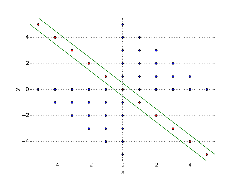
Figure 1: Example program. The right side shows some of the good and bad states of the program, in blue and red respectively

Overview.  The high-level overview of our approach is as follows: good and bad states are sampled by running the program on different initial states. Next, a numeric abstract domain that is likely to contain the invariant is chosen manually. We use disjunctions of octagons by default. For each hyperplane (up to translation) in the domain we add a new “feature” to each of the sample points corresponding to the distance to that hyperplane. A Decision Tree (DT) learning algorithm is then used to learn a DT that can separate the good and bad states in the sample, and this tree is converted into a formula that is a candidate invariant. Finally, this candidate invariant is passed to a theorem prover that verifies the correctness of the invariant. We now discuss these steps in detail.

Sampling.  The first step in our algorithm is to sample good and bad states of this program. We sample the good states by picking states satisfying the precondition, running the program from these states and collecting all states reached. To sample bad states, we look at all points close to good states, run the program from these. If the loop exits within a bounded number of iterations and fails the assert, we mark all states reached as bad states. The sampled good and bad states are shown in Fig. 1.

Features.  The next step is to choose a candidate hyperplane set for the inequalities in the invariant. For most of our benchmarks, we used the octagon abstract domain, which consists of all linear inequalities of the form:

$$b_{i}\cdot x_{i}+b_{j}\cdot x_{j}\leq c\text{ where }1\leq i<j\leq d,\;b_{i},b_{j}\in\{-1,0,1\},\text{ and }c\in\mathbb{Z}.$$

We then let $H=\{\vec{w_{1}},\vec{w_{2}},\dotsc\}$ be the set of hyperplane slopes for this domain. Then we transform our sample points (both good and bad) according to these slopes. For each sample point $\vec{x}$, we get a new point $\vec{z}$ given by $z_{i}=\vec{x}\cdot\vec{w_{i}}$. In our example, the octagon slopes $H$ and some of our transformed good and bad points are

$$\small H=\begin{bmatrix}[r]1&0\\ 0&1\\ 1&-1\\ 1&1\\ \end{bmatrix},\qquad\text{and}\qquad X\cdot H^{T}=\begin{bmatrix}[r]0&1\\ 1&0\\ -1&0\\ \lx@intercol\hfil\dots\hfil\lx@intercol\\ 0&0\\ 2&-2\\ -1&1\\ \lx@intercol\hfil\dots\hfil\lx@intercol\\ \end{bmatrix}\cdot\begin{bmatrix}[r]1&0&1&1\\ 0&1&-1&1\\ \end{bmatrix}=\begin{bmatrix}[r]0&1&-1&1\\ 1&0&1&1\\ -1&0&-1&-1\\ \lx@intercol\hfil\dots\hfil\lx@intercol\\ 0&0&0&0\\ 2&-2&4&0\\ -1&1&-2&0\\ \lx@intercol\hfil\dots\hfil\lx@intercol\end{bmatrix}\enspace.$$

Learning the DT.  After this transformation, we run a Decision Tree learning algorithm on the processed data. A DT (see Fig. 2 for an example) is a concise way to represent a set of rules as a binary tree. Each inner node is labeled by a feature and a threshold. Given a sample point and its features, we evaluate the DT by starting at the root and taking the path given by the rules: if the features is less than or equal to the threshold, we go to the left child, otherwise the right. Leaves specify the output label on that point. Most DT learning algorithms start at an empty tree, and greedily pick the best feature to split on at each node. From the good and bad states listed above, we can easily see that a good feature to split on must be the last one, as all bad states have the last column 0. Indeed, the first split made by the DT is to split on $z_{4}$ at $-0.5$. Since $w_{4}=(1,1)$, this split corresponds to the linear inequality $x+y\leq-0.5$. Now, half the good states are represented in the left child of the root (corresponding to $z_{4}\leq-0.5$). The right child contains all the bad states and the other half of the good states. So the algorithm leaves the left child as is and tries to find the best split for the right child. Again, we see the same pattern with $z_{4}$, and so the algorithm picks the split $z_{4}<1$. Now, all bad states fall into the left child, and all good states fall into the right child, and we are done. The computed DT is shown in Fig. 2.

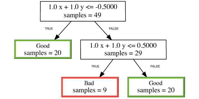
Figure 2: Decision tree learned from the program and sample data in Fig. 1

Finally, we need to convert the DT back into a formula. To do this, we can follow all paths from the root that lead to good leaves, and take the conjunction of all inequalities on the path, and finally take the disjunction of all such paths. In our example, we get the candidate invariant:

$$(x+y\leq-0.5)\vee(x+y>-0.5\wedge x+y>0.5)\enspace.$$

This can be simplified to $(x+y\neq 0)$.

Verifying the Candidate Invariant.  Our program is then annotated with this invariant and passed to a theorem prover to verify that the invariant is indeed sufficient to prove the program correct.

3 Preliminaries

Problem Statement.  We think of programs as transition systems $P=(S,R,\mathsf{init},\mathsf{safe})$, where $S$ is a set of states, $R\subseteq S\times S$ is a transition relation on the states, $\mathsf{init}\subseteq S$ is a set of initial states, and $\mathsf{safe}\subseteq S$ is the set of safe states that we want our program to remain within.

For any set of states $X$, the set $\mathsf{post}(X)$ represents all the successor states with respect to $R$. More formally,

$$\mathsf{post}(X)=\{\,x^{\prime}\mid\exists x\in X.\,R(x,x^{\prime})\,\}\enspace.$$

Then, we can define the set of reachable states of the program (the good states) to be the least fixed point,

$$\mathsf{good}=\mathsf{lfp}(\lambda X.\,\mathsf{init}\cup\mathsf{post}(X))\enspace.$$

Similarly, we can define

$$\mathsf{pre}(X)=\{\,x\mid\exists x^{\prime}\in X.\,R(x,x^{\prime})\,\}\quad\text{and}\quad\mathsf{bad}=\mathsf{lfp}(\lambda X.\,\mathsf{error}\cup\mathsf{pre}(X)),$$

where $\mathsf{error}$ is the complement of $\mathsf{safe}$. Then we see that the program is correct, with respect to the safety property given by $\mathsf{safe}$, if $\mathsf{good}\cap\mathsf{bad}=\emptyset$. Thus, our task is to separate the good states from the bad states.

One method to show that these sets are disjoint is to show the existence of a safe inductive invariant. A safe inductive invariant is a set $\mathsf{inv}$ that satisfies the following three properties:

• $\mathsf{init}\subseteq\mathsf{inv}$,

• $\mathsf{post}(\mathsf{inv})\subseteq\mathsf{inv}$,

• $\mathsf{inv}\subseteq\mathsf{safe}$.

It is easy to see that these conditions imply, in particular, that $\mathsf{inv}$ separates the good and bad states: $\mathsf{good}\subseteq\mathsf{inv}$ and $\mathsf{inv}\cap\mathsf{bad}=\emptyset$.

Invariant Generation as Binary Classification.  The set up for most machine learning problems is as follows. We have an input space ${\cal X}$ and an output space ${\cal Y}$, and one is given a set of samples $X\subseteq{\cal X}$ that are labeled by some unknown function $f:{\cal X}\to{\cal Y}$. We fix a hypothesis set ${\cal H}\subseteq{\cal Y}^{{\cal X}}$, and the aim is to find the hypothesis $h\in{\cal H}$ that most closely approximates $f$. The samples are often given in terms of feature vectors, and thus a sample $\vec{x}$ can be thought of as a point in some $d$-dimensional space.

Binary classification is a common instance of this problem, where the labels are restricted to a binary set ${\cal Y}=\{0,1\}$. Following [31], we view the problem of computing a safe inductive invariant for a program $P=(S,R,\mathsf{init},\mathsf{safe})$ as a binary classification problem by defining the input space as the set of all program states ${\cal X}=S$. Sample states $\vec{x}\in\mathsf{bad}$ are labeled by $0$ and $\vec{x}\in\mathsf{good}$ are labeled by $1$. Thus, the unknown function $f$ is the characteristic function of the set of good states. The hypothesis to be learned is a safe inductive invariant. Note that if sampling the program shows that some state $\vec{x}$ is both $\mathsf{good}$ and $\mathsf{bad}$, there exists no safe inductive invariant, and the program is shown to be unsafe. Hence, we assume that the set of sample states can be partitioned into good and bad states.

Decision Trees.  Instead of considering a hypothesis space that can represent arbitrary invariants, we restrict it to a specific abstract domain, namely those invariants that can be represented using decision trees. A Decision Tree (DT) [23] is a binary tree that represents a Boolean function. Each inner node $v$ of $T$ is labeled by a decision of the form $x_{i}\leq t$, where $x_{i}$ is one of the input features and $t$ is a real valued threshold. We denote this inequality by $v.\mathsf{cond}$. We denote the left and right children of an inner node by $v.\mathsf{left}$ and $v.\mathsf{right}$ respectively. Each leaf $v$ is labeled by an output $v.\mathsf{label}$. To evaluate an input, we trace a path down from the root node $T.\mathsf{root}$ of the tree, going left at each inner node if the decision is true, and right otherwise. The output of the tree on this input is the label of the leaf reached by this process. The hypothesis set corresponding to all DTs is thus arbitrary Boolean combinations of linear inequalities of the form $x_{i}\leq t$ (axis-aligned hyperplanes).

As one can easily see, many DTs can represent the same underlying function. However, the task of finding the smallest (in terms of number of nodes) DT for a particular function can be shown to be NP-complete [19]. Standard algorithms to learn DTs work by greedily selecting at each node the co-ordinate and threshold that separates the remaining training data best [27, 7]. This procedure is followed recursively until all leaves have samples labeled by a single class.

The criterion for separation is normally a measure such as conditional entropy. Entropy is a commonly used measure of uncertainty in a system. It is a function that is low when the system is homogeneous (in this case, think of when all samples reaching a node have the same label), and high otherwise. Conditional entropy, analogously, measures how homogeneous the samples are after choosing a particular co-ordinate and threshold. More formally, at each node, we look at the samples that reach that node, and define the conditional entropy of splitting feature $x_{i}$ at threshold $t$ as

$$H(y|x_{i}:t)={} p(x_{i}<t)H(y|x_{i}<t)+p(x_{i}\geq t)H(y|x_{i}\geq t),$$

$$\text{where}\quad H(y|x_{i}<t)={} -\sum_{a\in{\cal Y}}p(y=a|x_{i}<t)\log p(y=a|X_{i}<t),$$

and $p(A)$ is the empirical probability, i.e., the fraction of sample points reaching this node that satisfy the condition $A$. $H(y|x_{i}\geq t)$ is defined similarly to $H(y|x_{i}<t)$. Note that if a particular split perfectly separates good and bad samples, then the conditional entropy is 0. The greedy heuristic is to pick the feature and split that minimize the conditional entropy. There are other measures as well, such as the Gini index, which is used by the DT learner we used in our experiments [25].

4 Algorithm

We now present our DT-learning algorithm. We assume that we have black box procedures for sampling points from the given program, and for getting a set of slopes from a chosen abstract domain. To this end, let Sampler be a procedure that takes a program and returns an $n\times d$ matrix $X$ of $n$ sample points, and an $n$-dimensional vector $\vec{y}$ corresponding to the label of each sample point (1 for good states, 0 otherwise). Similarly, let Slopes be a procedure that takes a program and returns an $m\times d$ matrix $H$ of $m$ hyperplane slopes. We describe the actual procedures used in our experiments in Section 5.1.

Our final algorithm is surprisingly simple, and is given in Algorithm 1. We get the sample points and the slopes from the helper functions mentioned above, and then transform the sample points according to the slopes given. We run a standard DT learning algorithm on the transformed sample to obtain a tree that classifies all samples correctly. The tree is then transformed into a formula that is a candidate invariant, by a simple procedure DTtoForm. Finally, the program is annotated with the candidate invariant and verified. This final step is realized by another black box procedure IsInvariant, which checks that the invariant satisfies the three conditions necessary to be a safe inductive invariant. For example, this can be done by encoding $\mathsf{init},\mathsf{inv},\mathsf{post}$ and $\mathsf{safe}$ as SMT formulas and feeding the three conditions into an SMT solver.

def DTInv ($P$ : program): safe inductive invariant for $P$ or $\mathsf{fail}$ ${}=$

       val $X,\vec{y}=\textnormal{{Sampler(}}\textnormal{{P}}\textnormal{{)}}$

       val $H=\textnormal{{Slopes(}}\textnormal{{P}}\textnormal{{)}}$

       val $Z=X\cdot H^{T}$

       val $T=$ LearnDT($Z$, $\vec{y}$)

       val $\varphi=\textnormal{{DTtoForm(}}\textnormal{{T.{{root}}}}\textnormal{{)}}$

       if IsInvariant($P$, $\varphi$) then $\varphi$

       else $\mathsf{fail}$

      

def DTtoForm (v: node of a decision tree): formula represented by subtree rooted at v${}=$

       if v is a leaf then v.label

       else $(\textnormal{{v}}.\textnormal{{cond}}\land\textnormal{{DTtoForm(}}\textnormal{{{{v}}.{{left}}}}\textnormal{{)}}\lor\neg\textnormal{{v}}.\textnormal{{cond}}\land\textnormal{{DTtoForm(}}\textnormal{{{{v}}.{{right}}}}\textnormal{{)}})$

      

Algorithm 1 $\mathtt{DTInv}$: Invariant generation algorithm using DT learning

To convert the DT into a formula, we note that the set of states that reach a particular leaf is given by the conjunction of all predicates on the path from the root to that leaf. Thus, the set of all states classified as good by the DT is the disjunction of the sets of states that reach all the good leaves. A simple conversion is then to take the disjunction over all paths to good leaves of the conjunction of all predicates on such paths. The procedure DTtoForm computes this formula recursively by traversing the learned DT. Since the tree was learnt on the transformed sample data, the predicate at each node of the tree will be of the form $z_{i}\leq c$ where $z_{i}$ is one of the columns of $Z$ and $c$ is a constant. Since $Z=X\cdot H^{T}$, we know that $z_{i}(\vec{x})=\vec{x}\cdot\vec{w_{i}}$ for a sample $\vec{x}$. Thus, the predicate is equivalent to $\vec{x}\cdot\vec{w_{i}}\leq c$, which is a linear inequality in the program variables. Combining this with the conversion procedure above, we see that our algorithm outputs an invariant which is a Boolean combination of linear inequalities over the numerical program variables.

Soundness.  From the above discussion, we see that the formula $\varphi$ returned by the procedure DTtoForm is of the required format. Moreover, we assume that the procedure IsInvariant is correct. Thus, we can say that our invariant generation procedure DTInv is sound: if it terminates successfully, it returns a safe inductive invariant.

Probabilistic Completeness.  It is harder to prove that such invariant generation algorithms are complete. We see that the performance of our algorithm depends heavily on the sample set, if the sample is inadequate, it is impossible for the DT learner to learn the underlying invariant. One could augment our algorithm with a refinement loop, which would make the role of the sampler less pronounced, for if the invariant is incorrect, the theorem prover will return a counterexample that could potentially be added to the sample set and we can re-run learning. However, we find in practice that we do not need a refinement loop if our sample set is large enough.

We can justify this observation using Valiant’s PAC (probably approximately correct) model [33]. In this model, one can prove that an algorithm that classifies a large enough sample of data correctly has small error on all data, with high probability. It must be noted that one key assumption of this model is that the sample data is drawn from the same distribution as the underlying data, an assumption that is hard to justify in most of its applications, including this one. In practice however, PAC learning algorithms are empirically successful on a variety of applications where the assumption on distribution is not clearly true. Formally, we can give a generalization guarantee for our algorithm using this result of Blumer et al. [6]:

Theorem 4.1

A learning algorithm for a hypothesis class ${\cal H}$ that outputs a hypothesis $h\in{\cal H}$ will have true error at most $\epsilon$ with probability at least $1-\delta$ if $h$ is consistent with a sample of size $\max(\frac{4}{\epsilon}\log\frac{2}{\delta},\frac{8VC({\cal H})}{\epsilon}\log\frac{13}{\epsilon})$.

In the above theorem, a hypothesis is said to be consistent with a sample if it classifies all points in the sample correctly. The quantity $VC({\cal H})$ is a property of the hypothesis class called the Vapnik-Chervonenkis (VC) dimension, and is a measure of the expressiveness of the hypothesis class. As one might imagine, more complex classes lead to a looser bound on the error, as they are more likely to over-fit the sample and less likely to generalize well.

Thus, it suffices for us to bound the VC dimension of our hypothesis class, which is all finite Boolean combinations of hyperplanes in $d$ dimensions. The VC dimension of a class ${\cal H}$ is defined as the cardinality of the largest set of points that ${\cal H}$ can shatter. A set of points is said to be shattered by a hypothesis class ${\cal H}$ if for every possible labeling of the points, there exists a hypothesis in ${\cal H}$ that is consistent with it. Unfortunately, DTs in all their generality can shatter points of arbitrarily high cardinality. Given any set of $m$ points, we can construct a DT with $m$ leaves such that each point ends up at a different leaf, and now we can label the leaf to match the labeling given.

Since in practice we will not be learning arbitrarily large trees, we can restrict our algorithm a-priori to stop growing the tree when it reaches $K$ nodes, for some fixed $K$ independent of the sample. Now one can use a basic, well-known lemma from [24] combined with Sauer’s Lemma [29] to get that the VC dimension of bounded decision trees is $O(Kd\log K)$. Combining this with Theorem 4.1, we get the following polynomial bound for probabilistic completeness:

Theorem 4.2

Under the assumptions of the PAC model, the algorithm DTInv returns an invariant that has true error at most $\epsilon$ with probability at least $1-\delta$, given that its sample size is $O(\frac{1}{\epsilon}Kd\log K\log\frac{1}{\delta})$ .

Complexity.  The running time of our algorithm depends on many factors such as the running time of the sampling (which in turn depends on the benchmark being considered), and so is hard to measure precisely. However, the running time of the learning routine for DTs is $O(mn\log(n))$, where $m$ is the number of hyperplane slopes in $H$ and $n$ is the number of sample points [7, 25]. The learning algorithm therefore scales well to large sets of sample data.

Nonlinear invariants.  An important property of our algorithm is that it generalizes elegantly to nonlinear invariants as well. For example, if a particular program requires invariants that reason about $(x\mod 2)$ for some variable $x$, then we can learn such invariants as follows: given the sampled states $X$, we add to it a new column that corresponds to a variable $x^{\prime}$, such that $x^{\prime}=x\mod 2$. We then run the rest of our algorithm as before, but in the final invariant, replace all occurrences of $x^{\prime}$ by $(x\mod 2)$. As is easy to see, this procedure correctly learns the required nonlinear invariant. We have added this feature to our implementation, and show that it works on benchmarks requiring these nonlinear features (see Section 5.2).

5 Implementation and Evaluation

5.1 Implementation

We implemented our algorithm in Python, using the scikit-learn library’s decision tree classifier [25] as the DT learner LearnDT. This implementation uses the CART algorithm from [7] which learns in a greedy manner as described in Section 3, and uses the Gini index.

We implemented a simple and naive Sampler: we considered all states that satisfied the precondition where the value of every variable was in the interval $[-L,L]$. For these states, we ran the program with a bound $I$ on the number of iterations of loops, and collected all states reached as good states. To find bad states, we looked at all states that were a margin $M$ away from every good state, ran the program from this state (again with at most $I$ iterations), and if the program failed an assertion, we collected all the states on this path as bad states. The bounds $L,I,M$ were initialized to low values and increased until we had sampled enough states to prove our program correct.

For the Slopes function, we found that for most of the programs in our benchmarks it sufficed to consider slopes in the octagonal abstract domain. This consists of all vectors in $\{-1,0,1\}^{d}$ with at most two non zero elements. In a few cases, we needed additional slopes (see Table 1). For the programs hola15 and hola34, we used a class of slopes of vectors in $C^{d}$ where $C$ is a small set of constants that appear in the program, and their negations.

We also developed methods to learn the class of slopes needed by a program by looking at the states sampled. In [31], the authors suggest working in the null space of the good states, viewed as a matrix. This is because if the good states lie in some lower dimensional space, this would automatically suggest equality relationships among them that can be used in the invariant. It also reduces the running time of the learning algorithm. Inspired by this, we propose using Principal Component Analysis [20] on the good states to generate slopes. PCA is a method to find the basis of a set of points so as to maximize the variance of the points with respect to the basis vectors. For example, if all the good points lie along the line $2x+3y=4$, then the first PCA vector will be $(2,3)$, and intuition suggests that the invariant will use inequalities of the form $2x+3y<c$.

Finally, for the IsInvariant routine, we used the program verifier Boogie [4], which allowed us to annotate our programs with the invariants we verified. Boogie uses the SMT solver Z3 [12] as a back-end.

5.2 Evaluation

We compared our algorithm with a variety of other invariant inference tools and static analyzers. We mainly focused on ML-based algorithms, but also considered tools based on interpolation and abstract interpretation. Specifically, we considered:

• ICE [14]: an ML algorithm based on ICE-learning that uses an SMT solver to learn numerical invariants.

• MCMC [30]: an ML algorithm based on Markov Chain Monte Carlo methods. There are two versions of this algorithm, one that uses templates such as octagons for the invariant, and one with all constants in the slopes picked from a fixed bag of constants. The two algorithms have very similar characteristics. We ran both versions 5 times each (as they are randomized) and report the better average result of the two algorithms for each benchmark.

• SC [31]: an ML algorithm based on set cover. We only had access to the learning algorithm proposed in [31] and not the sampling procedure. To obtain a meaningful comparison, we combined it with the same sampler that we used in the implementation of our algorithm DTInv.

• CPAchecker [5]: a configurable software model checker. We chose the default analysis based on predicate abstraction and interpolation.

• UFO [2]: a software model checker that combines abstract interpretation and interpolation (denoted CPA).

• InvGen [18]: an inference tool for linear invariants that combines abstract interpretation, constraint solving, and testing.

For our comparison, we chose a combination of 22 challenging benchmarks from various sources. In particular, we considered a subset of the benchmarks from [31, 14, 18, 13]. We chose the benchmarks at random among those that were hard for at least one other tool to solve. Due to this bias in the selection, our experimental results do not reflect the average performance of the tools that we compare against. Instead, the comparison should be considered as an indication that our approach provides a valuable complementary technique to existing algorithms.

Name	Vars	Type	$\boldsymbol{|\varphi|}$	Samp	DT	SC	DTInv	ICE	MCMC	CPA	UFO	InvGen
Octagonal:
ex23[14]	4	conj.	3	0.10	0.01	4.73	0.11	8.82	0.01	19.77	1.50	0.02
fig6[14]	2	conj.	2	0.00	0.00	2.61	0.00	0.30	0.00	1.68	0.13	0.01
fig9[14]	2	conj.	2	0.00	0.01	2.31	0.01	0.33	0.00	1.73	0.13	0.01
hola10[13]	4	conj.	8	0.03	0.00	2.45	0.03	49.21	TO	2.03	F	F
nested2[31]	4	conj.	3	0.03	0.00	2.39	0.03	62.02	0.09	1.86	0.12	0.03
nested5[18]	4	conj.	4	2.48	0.02	MO	2.50	60.95	31.28*	2.08	0.35	0.03
fig1[14]	2	disj.	3	14.61	0.01	F	14.62	0.38	5.13	1.75	1.64	F
test1[31]	4	disj.	2	0.90	0.01	7.86	0.91	0.39	TO	1.71	F	0.04
cegar2[14]	3	ABC	5	0.03	0.01	2.64	0.04	4.86	17.30	1.97	0.18	F
gopan[31]	2	ABC	8	0.03	0.00	2.54	0.03	F	TO	63.85	58.29	F
hola18[13]	3	ABC	6	1.60	0.04	MO	1.64	TO	21.93*	TO	8.38	F
hola19[13]	4	ABC	7	0.19	0.01	3.47	0.20	F	TO	F	F	F
popl07[31]	2	ABC	7	0.03	0.00	2.72	0.03	F	TO	110.81	15.20	F
prog4[31]	3	ABC	8	2.32	0.02	MO	2.34	F	0.13	F	F	F
sum1[14]	3	ABC	6	0.01	0.01	2.61	0.02	1.32	29.04*	F	0.17	F
trex3[14]	8	ABC	9	8.44	0.06	MO	8.50	4.51	NA	F	0.18	F
Non octagonal:
hola15[13]	3	conj.	2	0.52	0.02	0.01	0.54	0.53	0.04	MO	0.13	0.02
Modulus:
hola02[13]	4	conj.	4	0.03	0.03	F	0.06	F	NA	F	F	F
hola06[13]	4	conj.	3	1.79	0.03	MO	1.82	F	NA	F	F	F
hola22[13]	4	conj.	5	0.04	0.00	F	0.04	F	NA	F	F	F
Non octagonal modulus:
hola34[13]	4	ABC	6	1.14	0.03	3.10	1.17	F	NA	F	F	F
Quadratic:
square	3	conj.	3	0.27	0.24	MO	0.51	F	NA	F	F	F

Table 1: Results of comparison. The table is divided according to what kinds of invariants the benchmark needed. The “Type” column denotes the Boolean structure of the invariant - conjunctive, disjunctive and arbitrary Boolean combination are denoted as conj., disj. and ABC respectively. The column $|\varphi|$ contains the number of predicates in the invariant found by DTInv.
The columns ’Samp’ and ’DT’ show the running time in seconds of our sampling and DT learning procedures respectively. We show SC next, as we only compare learning times with SC. Then follows the total time of our tool (DTInv), followed by those for other tools. Each entry of the tool columns shows the running time in seconds if a safe invariant was found, or otherwise one of the following entries. ’NA’: program contains arithmetic operations that are not supported by the tool; ’F’: analysis terminated without finding a safe invariant; ’TO’: timeout; ’MO’: out of memory. The times for MCMC have an asterisk if at least one of the repetitions timed out. In this case the number shown is the average of the other runs.

We ran our experiments on a machine with a quad-core 3.40GHz CPU and 16GB RAM, running Ubuntu GNU/Linux. For the analysis of each benchmark, we used a memory limit of 8GB and a timeout of 5 minutes. The results of the experiment are summarized in Table 1. Here are the observations from our experiments (we provide more in-depth explanations for these observations in the next section, where we discuss related work in more detail):

• Our algorithm DTInv seems to learn complex Boolean invariants as easily as simple conjunctions.

• ICE seems to struggle on programs that needed large invariants. For some of these (gopan, popl07), this is because the constraint solver runs out of time/memory, as the constants used in the invariants are also large. For hola19 and prog4, ICE stops because the tool has an inbuilt limit for the complexity of Boolean templates.

• However, ICE solves sum1 and trex3 quickly, even though they need many predicates, because the constant terms are small, so this space is searched first by ICE.

• Similarly, we notice that MCMC has difficulty finding large invariants, again because the search space is huge.

• SC’s learning algorithm is consistently slower than DTInv, due to its higher running time complexity. It also runs out of memory for large sample sizes.

• DTInv is able to easily handle benchmarks that CPA, UFO and InvGen struggle on. This is mainly because they are specialized for reasoning about linear invariants, and have issues dealing with invariants that have complicated Boolean structure.

We also learned some of the weak points in our current approach:

• DTInv is slow in processing fig1 and prog4, both of which are handled by at least one other tool without much effort. However, we note that most of this time is spent in the sampling routine, which is currently a naive implementation. We therefore believe that DT learning could benefit from a combination with a static analysis that provides approximations of the good and bad states to guide the sampler.

• We also note that the method of “constant slopes” which we used to handle the non octagonal benchmarks (hola15, hola34) is ad-hoc, and might not work well for larger benchmarks.

Beyond octagons.  As mentioned in Section 4, we implemented a feature to learn certain nonlinear invariants. We were able to verify some benchmarks that needed reasoning about the modulus of certain variables, as shown in Table 1. Finally, we show one example where we were able to infer a nonlinear invariant (specifically $s=i^{2}\wedge i\leq n$ for square).

We believe our experiments show that Decision Trees are a natural representation for invariants, and that the greedy learning heuristics guide the algorithm to discover simple invariants of complex structures without additional overhead.

6 Related Work and Conclusions

Our experimental evaluation compared against other algorithms for invariant generation. We discuss these algorithms in more detail. Sharma et. al. [31] used the greedy set cover algorithm SC to learn invariants in the form of arbitrary Boolean combinations of linear inequalities. Our algorithm based on decision trees is simpler than the set cover algorithm, works better on our benchmarks (which includes most of the benchmarks from [31]), and scales much better to large sample sets of test data. The improved scalability is due to the better complexity of DT learners. The running time of our learning algorithm is $\mathcal{O}(mn\log(n))$ where $m$ is the number of features/hyperplane slopes that we consider, and $n$ the number of sample points. On the other hand, the set cover algorithm has a running time of $\mathcal{O}(mn^{3})$. This is because the greedy algorithm for set cover takes time $\mathcal{O}(hn^{2})$ where $h$ is the number of hyperplanes, and [31] considers one hyperplane for every candidate slope and sample point, yielding $h=mn$.

When invariant generation is viewed as binary classification, then there is a problem in the refinement loop: if the learned invariant is not inductive, it is unclear whether the counterexample model produced by the theorem prover should be considered a “bad” or a “good” state. The ICE-learning framework [14] solves this problem by formulating invariant generation as a more general classification problem that also accounts for implication constraints between points. We note that our algorithm does not fit within this framework, as we do not have a refinement loop that can handle counterexamples in the form of implications. However, we found in our experiments that we did not need any refinement loop as our algorithm was able to infer correct invariants directly after sampling enough data. Nevertheless, considering an ICE version of DT learning is interesting as sampling without a refinement loop becomes difficult for more complex programs.

The paper [14] also proposes a concrete algorithm for inferring linear invariants that fits into the ICE-learning framework (referred to as ICE in our evaluation). If we compare the complexity of learning given a fixed sample, our algorithm performs better than [14] both in terms of running time and expressiveness of the invariant. The ICE algorithm of [14] iterates through templates for the invariant. This iteration is done by dovetailing between more complex Boolean structures and increasing the range of the thresholds used. For a fixed template, it formulates the problem of this template being consistent with all given samples as a constraint in quantifier-free linear integer arithmetic. Satisfiability of this constraint is then checked using an SMT solver. We note that the size of the generated constraint is linear in the sample size, and that solving such constraints is NP-complete. In comparison, our learning is sub-quadratic time in the sample size. Also, we do not need to fix templates for the Boolean structure of the invariant or bound the thresholds a priori. Instead, the DT learner automatically infers those parameters from the sample data.

Another ICE-learning algorithm based on randomized search was proposed in [30] (the algorithm MCMC in our evaluation). This algorithm searches over a fixed space of invariants $S$ that is chosen in advance either by bounding the Boolean structure and coefficients of inequalities, or by picking some finite sub-lattice of an abstract domain. Given a sample, it randomly searches using a combination of random walks and hill climbing until it finds a candidate invariant that satisfies all the samples. There is no obvious bound on the time of this search other than the trivial bound of $|S|$. Again, we have the advantage that we do not have to provide templates of the Boolean structure and the thresholds of the hyperplanes. These parameters have to be fixed for the algorithm in [30]. Furthermore, the greedy nature of DT learning is a heuristic to try simpler invariants before more complex ones, and hence the invariants we find for these benchmarks are often much simpler than those found by MCMC.

Decision trees have been previously used for inferring likely preconditions of procedures [28]. Although this problem is related to invariant generation, there are considerable technical differences to our algorithm. In particular, the algorithm proposed in [28] only learns formulas that fall into a finite abstract domain (Boolean combinations of a given finite set of predicates), whereas we use decision trees to learn more general formulas in an infinite abstract domain (e.g., unions of octagons).

We believe that the main value of our algorithm is its ability to infer invariants with a complex Boolean structure efficiently from test data. Other techniques for inferring such invariants include predicate abstraction [16] as well as abstract interpretation techniques such as disjunctive completion [10]. However, for efficiency reasons, many static analyses are restricted to inferring conjunctive invariants in practice [3, 11]. There exist techniques for recovering loss of precision due to imprecise joins using counterexample-guided refinement [26, 1, 21]. In the future, we will explore whether DL learning can be used to complement such refinement techniques for static analyses.

References

- [1] A. Albarghouthi, A. Gurfinkel, and M. Chechik. Craig interpretation. In SAS, volume 7460 of LNCS, pages 300–316. Springer, 2012.
- [2] A. Albarghouthi, A. Gurfinkel, Y. Li, S. Chaki, and M. Chechik. UFO: verification with interpolants and abstract interpretation - (competition contribution). In TACAS, volume 7795 of LNCS, pages 637–640. Springer, 2013.
- [3] T. Ball, A. Podelski, and S. K. Rajamani. Boolean and cartesian abstraction for model checking C programs. In TACAS, volume 2031 of LNCS, pages 268–283. Springer, 2001.
- [4] M. Barnett, B. E. Chang, R. DeLine, B. Jacobs, and K. R. M. Leino. Boogie: A modular reusable verifier for object-oriented programs. In FMCO 2005, Revised Lectures, pages 364–387, 2005.
- [5] D. Beyer and M. E. Keremoglu. Cpachecker: A tool for configurable software verification. In CAV, volume 6806 of LNCS, pages 184–190. Springer, 2011.
- [6] A. Blumer, A. Ehrenfeucht, D. Haussler, and M. K. Warmuth. Learnability and the vapnik-chervonenkis dimension. J. ACM, 36(4):929–965, 1989.
- [7] L. Breiman, J. H. Friedman, R. A. Olshen, and C. J. Stone. Classification and Regression Trees. Wadsworth, 1984.
- [8] E. M. Clarke, O. Grumberg, S. Jha, Y. Lu, and H. Veith. Counterexample-guided abstraction refinement. In CAV, volume 1855 of LNCS, pages 154–169. Springer, 2000.
- [9] P. Cousot and R. Cousot. Abstract interpretation: a unified lattice model for static analysis of programs by construction or approximation of fixpoints. In POPL, 1977.
- [10] P. Cousot and R. Cousot. Systematic design of program analysis frameworks. In POPL, pages 269–282, San Antonio, Texas, 1979. ACM.
- [11] P. Cousot, R. Cousot, J. Feret, L. Mauborgne, A. Miné, D. Monniaux, and X. Rival. The astreé analyzer. In ESOP, volume 3444 of LNCS, pages 21–30. Springer, 2005.
- [12] L. De Moura and N. Bjørner. Z3: An Efficient SMT Solver. In TACAS, LNCS, pages 337–340. Springer, 2008.
- [13] I. Dillig, T. Dillig, B. Li, and K. L. McMillan. Inductive invariant generation via abductive inference. In OOPSLA, pages 443–456. ACM, 2013.
- [14] P. Garg, C. Löding, P. Madhusudan, and D. Neider. ICE: A robust framework for learning invariants. In CAV, volume 8559 of LNCS, pages 69–87. Springer, 2014.
- [15] P. Godefroid, A. V. Nori, S. K. Rajamani, and S. Tetali. Compositional may-must program analysis: unleashing the power of alternation. In POPL, pages 43–56. ACM, 2010.
- [16] S. Graf and H. Saidi. Construction of abstract state graphs with PVS. In CAV, pages 72–83, 1997.
- [17] B. S. Gulavani, T. A. Henzinger, Y. Kannan, A. V. Nori, and S. K. Rajamani. SYNERGY: a new algorithm for property checking. In FSE, pages 117–127, 2006.
- [18] A. Gupta and A. Rybalchenko. Invgen: An efficient invariant generator. In CAV, volume 5643 of LNCS, pages 634–640. Springer, 2009.
- [19] L. Hyafil and R. L. Rivest. Constructing optimal binary decision trees is np-complete. Inf. Process. Lett., 5(1):15–17, 1976.
- [20] I. T. Jolliffe. Principal Component Analysis. Springer Verlag, 1986.
- [21] B. Kafle and J. P. Gallagher. Tree automata-based refinement with application to horn clause verification. In VMCAI, LNCS. Springer, 2015. To appear.
- [22] A. Miné. The octagon abstract domain. Higher-Order and Symbolic Computation, 19(1):31–100, 2006.
- [23] T. M. Mitchell. Machine learning. McGraw Hill series in computer science. McGraw-Hill, 1997.
- [24] M. Mohri. Foundations of machine learning 2014: Homework assignment 1 (problem c)., Oct. 2014.
- [25] F. Pedregosa, G. Varoquaux, A. Gramfort, V. Michel, B. Thirion, O. Grisel, M. Blondel, P. Prettenhofer, R. Weiss, V. Dubourg, J. Vanderplas, A. Passos, D. Cournapeau, M. Brucher, M. Perrot, and E. Duchesnay. Scikit-learn: Machine learning in Python. Journal of Machine Learning Research, 12:2825–2830, 2011.
- [26] A. Podelski and T. Wies. Counterexample-guided focus. In POPL, pages 249–260. ACM, 2010.
- [27] J. R. Quinlan. C4.5: Programs for Machine Learning. Morgan Kaufmann, 1993.
- [28] S. Sankaranarayanan, S. Chaudhuri, F. Ivancic, and A. Gupta. Dynamic inference of likely data preconditions over predicates by tree learning. In ISSTA, pages 295–306, 2008.
- [29] N. Sauer. On the density of families of sets. J. Comb. Theor. Ser. A, 25:80–83, 1972.
- [30] R. Sharma and A. Aiken. From invariant checking to invariant inference using randomized search. In CAV, volume 8559 of LNCS, pages 88–105. Springer, 2014.
- [31] R. Sharma, S. Gupta, B. Hariharan, A. Aiken, and A. V. Nori. Verification as learning geometric concepts. In F. Logozzo and M. Fähndrich, editors, SAS, volume 7935 of Lecture Notes in Computer Science, pages 388–411. Springer, 2013.
- [32] R. Sharma, A. V. Nori, and A. Aiken. Interpolants as classifiers. In CAV, volume 7358 of LNCS, pages 71–87. Springer, 2012.
- [33] L. G. Valiant. A theory of the learnable. Commun. ACM, 27(11):1134–1142, 1984.
- [34] G. Yorsh, T. Ball, and M. Sagiv. Testing, abstraction, theorem proving: better together! In ISSTA, pages 145–156. ACM, 2006.