Robust Face Recognition by Constrained Part-based Alignment

Abstract

Developing a reliable and practical face recognition system is a long-standing goal in computer vision research. Existing literature suggests that pixel-wise face alignment is the key to achieve high-accuracy face recognition. By assuming a human face as piece-wise planar surfaces, where each surface corresponds to a facial part, we develop in this paper a Constrained Part-based Alignment (CPA) algorithm for face recognition across pose and/or expression. Our proposed algorithm is based on a trainable CPA model, which learns appearance evidence of individual parts and a tree-structured shape configuration among different parts. Given a probe face, CPA simultaneously aligns all its parts by fitting them to the appearance evidence with consideration of the constraint from the tree-structured shape configuration. This objective is formulated as a norm minimization problem regularized by graph likelihoods. CPA can be easily integrated with many existing classifiers to perform part-based face recognition. Extensive experiments on benchmark face datasets show that CPA outperforms or is on par with existing methods for robust face recognition across pose, expression, and/or illumination changes.

I Introduction

Developing a reliable and practical face recognition system is a long-standing goal in computer vision research. A tremendous amount of works have been done in the past three decades, however, most of them can only work well in controlled scenarios. In more practical scenarios, performance of these existing methods degrades drastically due to face variations caused by illumination, pose, and/or expression changes [1].

To handle the variation caused by illumination change, the methods of Lee et al. [2], Wagner et al. [3], motivated by the illumination cone model [4, 5], used multiple carefully chosen face images of varying illuminations per subject as gallery. Given a probe face of unknown subject under arbitrary illumination, face images under this specific illumination can be generated in the gallery to match with the probe face. When multiple gallery images of such kind are not available, alternative methods [6, 7] considered extracting illumination invariant features for face recognition.

To address pose or expression variations, earlier approaches extend classic subspace or template based face recognition methods [8, 9]. The use of these methods is rather restricted due to their dependence on the availability of gallery images of multiple facial poses or expressions. Recent approaches consider more practical scenarios where only face images under the normal condition (frontal view and neutral expression) are assumed to be available in the gallery. To recognize a probe face with pose or expression changes, they either identified an implicit identity feature/representation of the probe face [10, 11, 12], which is pose- and expression-invariant, or explicitly estimate global or local mappings of facial appearance so that a virtual face under the normal condition can be synthesized for recognition [13, 14, 15, 16, 17]. However, most of these methods are still far from practice since they assume both gallery and probe face images have been manually aligned into some canonical form, and they cannot generally cope with illumination variation either.

In literature, the most popular approaches for automatic face alignment across pose or expression are based on facial landmark localization, e.g., the Active Appearance Models (AAMs) [18, 19] and elastic graph matching (EGM) [20]. AAMs and EGM used densely-connected elastic graphs, which however, are difficult to optimize in that the solutions are likely to be trapped into undesirable local minima. Consequently, localized landmarks using these methods are often not accurate enough, especially when applied to unseen face images. To improve the localization accuracy, an explicit shape constraint for graph nodes was considered in the constrained local models (CLMs) [21]. CLMs [21, 22, 23] are still based on densely-connected graph models, and their shape constraints are over-simplified so that the dependency among different graph nodes is ignored. Recently, deformable part-based models (DPMs) show their promise in many applications such as object detection [24] and facial landmark localization [25]. In particular, Zhu and Ramanan [25] adopted a tree-structured part model, which encodes node dependency while admitting efficient solutions. Such a tree model was used by Zhu and Ramanan [25] for facial landmark localization. Nevertheless, it cannot be readily extended for pixel-wise face alignment, and consequently for face recognition across pose or expression.

With the aim of developing a system that can simultaneously handle illumination variation and minor changes of pose and expression, Wagner et al. [3] recently leveraged sparsity optimization and a carefully prepared gallery set (multiple images of varying illuminations per subject), to align probe face images into a canonical form for better recognition. In particular, they assumed human face as a planar surface and chose a global similarity transformation for face alignment. This may be valid when probe faces are close to the normal condition. It is however a rather simplified assumption when there exist pose and/or expression changes. Indeed, a human face has non-planar geometry and non-rigid deformation. Some portions of the face (e.g., the nose region) undergo significant appearance changes as the pose varies, while other portions (e.g. the mouth region) deform significantly as expression changes. It is thus more appropriate to approximate a human face as a piece-wise planar surface, and correspondingly use piece-wise geometric transformation for face alignment.

Improving performance using enriched models is not an easy task in computer vision research. In fact, opposite effects often happen. As to the problems considered in this paper, we will show that by partitioning a human face as a collection of parts, and carefully characterizing the deformation relations among different parts, performance of face recognition across pose or expression can be significantly improved. In particular, we propose a Constrained Part-based Alignment (CPA) method for this task. Our method is partially motivated by the promise of piece-wise planar formulation and the explicit shape constraints used in CLMs [21, 22, 23] and DPMs [24, 25].

CPA partitions the object of interest, e.g., a human face, as a constellation of parts, and uses a similarity transformation to model the deformation of each part. A tree-structured shape model is used in CPA to constrain the relations among the deformations of different parts. A CPA model also has a batch of registered face images serving as the appearance evidence of each part. For a probe face image, all its parts are simultaneously aligned towards the registered model, by fitting them to the appearance evidence and penalizing the cost of violating the constraint from the tree-structured shape model. We formulate this objective as a norm minimization problem regularized by graph likelihoods, which is solved by an alternating method composed of two steps: one for aligning the parts, and the other for adjusting the configuration of the tree-structured model. The former can be reduced into a sequence of convex problems, while the latter admits efficient solutions by gradient decent methods. In this paper, we use the proposed CPA model for face recognition, where registered gallery images are taken as the appearance evidence, and a probe image is aligned using the CPA model. After alignment, most of the off-the-shelf face recognition methods can be readily used for part recognition.The overall decision is made by aggregating predictions from different parts by a plurality voting scheme. Robustness against illumination variation can also be achieved by choosing specific face recognition methods, e.g., [3, 26].

Richer models are often more difficult to train. For the proposed CPA model, both the appearance model and the tree-structured shape model need to be automatically learned. On the one hand, the appearance model is obtained by aligning the gallery images in batch with the constraint from a given shape model. In particular, we use low-rank and sparse matrix decomposition as the criteria to optimize batch alignment of each part, and globally regularize these individual problems of part alignment by graph likelihoods. On the other hand, the shape model is learned by the probabilistic inference based on given part constellations, where the maximum a posteriori (MAP) estimation is performed with the graph likelihoods and the given conjugate priors of the likelihoods. As the two problems are coupled, we solve them in a joint way. Moreover, we generalize our learning method to train a mixture of CPA models (mCPA) for better handling pose and expression variations.

Part-based face recognition methods [27, 28, 29, 30, 31] have shown improved performance over more standard approaches using holistic faces. However, existing part-based methods can only be applied when gallery and probe face images have been manually registered to each other. Our proposed CPA method enables this promising part-based strategy to be applicable in more practical scenarios, by automatically registering the gallery and probe face images in terms of deformable parts. In this paper, we present experiments on the Multi-PIE [32] and MUCT [33] datasets and show that our proposed CPA method can simultaneously and effectively handle illumination, pose, and/or expression variations.

• Comparing with the natural alternative methods that holistically align face images, followed by either holistic face recognition or part-based recognition, our method gives significantly improved performance.

• State-of-the-art pose-invariant face recognition method [34] relies on model learning using a large number of 3D face shapes, while training of our proposed CPA only requires 2D face images of a few subjects. Nevertheless, our method outperforms that of Li et al. [34]. when the degrees of pose change are within $\pm\mbox{15}^{\circ}$. This range of pose change is often encountered in practical access control scenarios, where test subjects would be cooperative with face recognition systems.

• Notably, while CPA is motivated to address the challenges of face recognition across pose/expression, it performs surprisingly well when probe face images are at frontal view and with neural expression. Our results in the frontal-view, neutral-expression, varying-illumination, and across-session setting of Multi-PIE dataset are better than all existing methods, and as high as 99.6%. This confirms that considering human face as a piece-wise planar surface and aligning it part-wisely are very effective for high-accuracy face recognition.

• We also empirically investigate the discriminative power of individual facial parts, and the robustness of our method against partial occlusion.

Details of these investigations are presented in Section VI.

The rest of this paper are organized as follows. Section II reviews more related work in addition to those discussed in Section I. Section III presents our proposed CPA model and how to use it for alignment of probe face images. Section IV combines CPA with existing methods for part-based face recognition. Details of CPA model learning are presented in Section V, where we also extend CPA to a mixture of CPA for better handling pose or expression variations. Intensive experiments are finally reported in Section VI to show the efficacy of our proposed method.

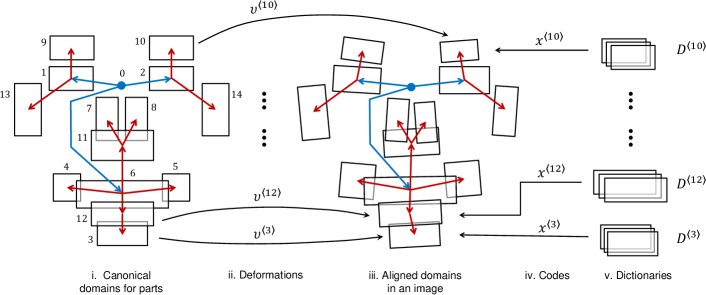
Figure 1: Illustration of a CPA model instance with 14 facial parts: Face is considered as a constellation of parts constrained by a tree structure, where each part corresponds to a pre-defined domain (i.e., shape and location) (Sub-figure i). For an image, deformations are computed (Sub-figure ii) for transforming the parts to the domains (Sub-figure iii) where they are aligned to the appearance evidence given by the linear combination (Sub-figure iv) of existing registered images (Sub-figure v).

II Related Work

As discussed in Section I, most of existing methods for face recognition across pose or expressions assume gallery and probe face images have been manually registered, and they can only be applied to controlled scenarios. In particular, Chai et al. [13] learned local patch based mapping relations from non-frontal pose to frontal pose by locally linear regression. Jorstad et al. [15] estimated pixel-wise registration from non-neutral expression to neutral expression by optical flow. Arashloo and Kittler [16] considered a Markov random field (MRF) model to regularize 2D displacements of local patches across different poses. For automatic face recognition across pose, given a probe face image, AAMs [18, 19] optimized localization of a set of facial landmarks to realize face alignment of pixel-level accuracy. However, the landmarks localized by AAMs are usually not accurate enough, and also the pixel-wise correspondence induced by matched landmarks are not consistent enough across different poses and expressions [35]. Among existing methods, maybe the most successful ones across pose and/or expression are based on 3D models [36, 35, 34]. In spite of their promise, their relying on 3D data makes them less relevant to the 2D techniques considered in this paper. However, we will show that our proposed CPA method compares favorably with them when the pose variations are in a reasonably confined range.

Deformable part models (DPM) have shown their success in object detection [24], facial landmark localization [25], and human pose estimation [37]. In particular, these methods optimize an objective function that scores both the appearance evidence and spatial constellation of the parts, where the former is scored by part detectors, and the latter is scored by a star- or tree-structured shape model, which constrain the pair-wise offsets of different parts. Our use of part-based models is different from the DPM based methods [24, 25, 37]. Our CPA method aims at pixel-wise image alignment rather than finding the bounding box of an object/part or locating a small amount of landmarks. We measure the appearance evidence of parts by their similarity to aligned galleries, and constrain the part deformation relations by a tree-structured shape model. Compared with shape constraints in DPMs [25, 37], our proposed one models more complex relations with the part constellation and holds strict probabilistic properties that are beneficial to the model learning.

Our method is also closely related to the work of Wagner et al. [3]. To cope with illumination variation, they used multiple gallery images of varying illuminations per subject. Our method also follows this strategy. However, we take a human face as a collection of parts rather than assuming it as a planar surface as in the method of Wagner et al. [3]. The piece-wise planar assumption used in our CPA model can handle much more complex facial appearance variations such as large pose and/or facial expression changes. Furthermore, we regularize the deformations of individual parts by a shape constraint in order to prevent the alignment from degenerated solutions. Such regularization term is absent in the method of Wagner et al. [3].

III CPA: Constrained Part-based Alignment

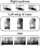
(a) Part dictionaries

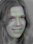
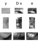
(b) Independent part alignment by Wagner et al. [3]’s method at Iteration 17

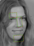
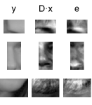
(c) Our CPA method at the converged stage

Figure 2: Part alignment obtained without/with a shape constraint. Parts are initialized at dashed red boxes, and aligned to the appearance evidence suggested by the part dictionaries. The solid green boxes denote the obtained domains of the parts. $y$ is the image cropped from an obtained domain, $D\cdot x$ is its best linear reconstruction with the given part dictinoary, and $e$ is the reconstruction error. The cropped images are normalized in terms of intensity for display convenience.

Assume we have face images of multiple subjects in a database, and these images have been registered into some canonical form, i.e., aligned to some template. The template we consider in this paper is composed of a collection of parts. These parts of varying sizes are spatially arranged in a proper manner so that overall they define our face template (Fig. 1-i). Suppose there are $m$ parts in the template. Each of the $m$ parts has its associated face region in each image in the database. We call these face regions associated with every $i^{\textrm{th}}$ part a part dictionary, which is denoted as $D^{\langle i\rangle}$ (Fig. 1-v). Let $y$ be a test face image that is not generally in the canonical form (e.g, due to pose change or misalignment). As the name of CPA suggests, constrained part-based alignment aims to align $y$ to the face template so that different face regions of $y$ are respectively registered with the corresponding parts of the face template. This part-based alignment can be realized by pursuing a set of transformations $\boldsymbol{\nu}=(\nu^{\langle 1\rangle},\nu^{\langle 2\rangle},\ldots,\nu^{\langle m\rangle})$ that act on the image domain of $y$ by $y\circ\nu^{\langle i\rangle}$, $i=1,\dots,m$.

To pursue $\boldsymbol{\nu}$, we consider techniques used in [26, 3]. In particular, Wright et al. [26], Wagner et al. [3] assumed there exist multiple registered face images of varying illuminations per subject in the database. A well-aligned test image could be represented by a linear combination of registered training images, plus a sparse error term to compensate for data corruption or various intra-subject variations. By leveraging the error sparsity assumption, Wagner et al. [3] optimized a holistic similarity transformation by solving a $\ell^{1}$-norm minimization problem. Extending techniques in [3] directly to part-based alignment gives the following objective

$$\min_{\underset{i=1,2,\ldots,m}{x^{\langle i\rangle},e^{\langle i\rangle},\boldsymbol{\nu}}}\;\sum_{i}^{m}\lambda^{\langle i\rangle}\|e^{\langle i\rangle}\|_{1}$$

$$\mathrm{s.t.}\quad y\circ\nu^{\langle i\rangle}=D^{\left\langle i\right\rangle}x^{\langle i\rangle}+e^{\langle i\rangle},$$ (2)

where $\|\cdot\|_{1}$ is the $\ell^{1}$-norm that encourages the sparsity of errors $\{e^{\langle i\rangle}\}_{i=1}^{m}$. $y\circ\nu^{\langle i\rangle}$ aligns the $i^{\textrm{th}}$ part of $y$, and $\{\lambda^{\langle i\rangle}\in\mathbb{R}_{+}\}_{i=1}^{m}$ balances the alignment errors of the $m$ parts. The matrix $D^{\langle i\rangle}$ is the $i^{\textrm{th}}$ part dictionary, whose columns represent the aligned regions of face images in the database, and $x^{\langle i\rangle}$ denotes the reconstruction coefficient.

The above direct extension of [3] essentially aligns the $m$ parts independently. Unfortunately, it empirically appears to be very unstable for facial part alignment. As shown in Fig. 2b, the parts may often drift away from their initialization to some more “flat” face regions. Indeed, alignment by optimizing $\nu^{\langle i\rangle}$ in $y\circ\nu^{\langle i\rangle}$ is a non-convex procedure (as explained in more details in Section III-B1). Compared with an entire face, individual parts contain less visual structure and thus alignment of them is prone to meaningless local minima. To overcome this problem, we consider in this paper incorporating some sort of global information of facial structure to regularize the deformations of individual parts. In particular, we are motivated by [25] to use a tree-structured shape model to constrain the difference of transformation parameters of different parts. We write $g\left(\boldsymbol{\nu},\mathcal{Z}\right)$ for the regularization term determined by the tree-structured shape model, where $\mathcal{Z}$ denotes model parameters in the form of a tuple. The tree-structured shape model is illustrated in Fig. 1 i - iii and will be elaborated in Section III-A. With consideration of the tree-structured shape constraint, we revise (2) to formulate the alignment objective of our proposed CPA model as

$$\min_{\underset{i=1,2,\ldots,m}{x^{\langle i\rangle},e^{\langle i\rangle},\boldsymbol{\nu}}}\;\sum_{i}^{m}\lambda^{\langle i\rangle}\|e^{\langle i\rangle}\|_{1}+\eta g\left(\boldsymbol{\nu},\mathcal{Z}\right)$$

$$\mathrm{s.t.}\quad y\circ\nu^{\langle i\rangle}=D^{\left\langle i\right\rangle}x^{\langle i\rangle}+e^{\langle i\rangle},$$ (3)

where $\eta\in\mathbb{R}_{+}$ weights the regularization term. The choice of $\{\lambda^{\langle i\rangle}\}_{i=1}^{m}$ will be addressed when we learn the CPA model in Section V. As shown in Fig. 2c, our proposed CPA method can produce very stable alignment results using the same part dictionaries (Fig. 2a) as independent part alignment does. In Fig. 3, we give all the part instances of the CPA model that are fitted to real face images. We note that CPA is not designed to produce a seamless face constituted by deformed individual parts, as AAMs [18, 19] can do. Instead, it aims to establish correspondence of facial parts across pose or expression so that face images with intra-subject variations can be matched at the part level to improve face recognition.

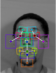
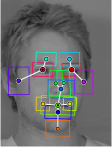
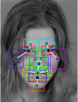
Figure 3: CPA model instances fitted to face images. Each facial part is denoted by a box in a specific color. The circled disk at its center denotes the associated tree node. The white solid lines denote the tree edges. Bigger nodes correspond to higher levels of the tree. The nodes with black dots are linked with the root node, which is not displayed in the figure.

III-A Tree-structured Shape Model

Let $(\mathcal{V},\mathcal{E})$ denote the tree, where $\mathcal{V}=\{0,1,2,\ldots,m\}$ is the vertex set, and $\mathcal{E}$ is the set of directed edges. $\mathcal{V}$ is composed of the nodes of the $m$ facial parts and a root node (the node “$0$”) corresponding to the holistic face. Every $i^{\textrm{th}}$ node takes $\nu^{\langle i\rangle}$ as its variables corresponding to the transformation parameters of the facial part. For the root node, we use $\nu^{\langle 0\rangle}=(0,0,0,0)^{T}$ when assuming the face at the global level has been registered into the canonical form, which suggests $(u,v)=\nu^{\langle 0\rangle}(u,v)$. We consider this simplified case in the following derivation of the tree-structured shape model.

In order to build a model on the tree, we first associate with each edge the difference of transformation parameters of its two end nodes. We then concretize $g\left(\boldsymbol{\nu},\mathcal{Z}\right)$ as follows. In particular, for the edge $(j,i)\in\mathcal{E}$ with parent node $j$ and child node $i$, we use a multivariate Gaussian distribution with mean $\mu^{\langle i\rangle}\in\mathbb{R}^{d}$ and precision $\Lambda^{\langle i\rangle}\in\mathbb{R}^{d\times d}$ to model the transformation difference $\nu_{\delta}^{\langle i\rangle}=\nu^{\langle i\rangle}-\nu^{\langle j\rangle}\in\mathbb{R}^{d}$, i.e., $p(\nu_{\delta}^{\langle i\rangle}|z^{\langle i\rangle})=\mathcal{N}(\nu_{\delta}^{\langle i\rangle};\mu^{\langle i\rangle},{\Lambda^{\langle i\rangle}}^{-1})$ with $z^{\langle i\rangle}=(\mu^{\langle i\rangle},\Lambda^{\langle i\rangle})$, where the Gaussian probability distribution function (PDF) is

$$\mathcal{N}(\nu_{\delta};\mu,\Lambda^{-1})=\frac{|\Lambda|^{1/2}}{(2\pi)^{d/2}}\exp\left\{-\frac{1}{2}(\nu_{\delta}-\mu)^{T}\Lambda(\nu_{\delta}-\mu)\right\}.$$ (4)

Thus, let $\mathcal{Z}=(z^{\langle 1\rangle},z^{\langle 2\rangle},\ldots,z^{\langle m\rangle})$ be a tuple of Gaussian parameters.

Since the definition of $p(\nu_{\delta}^{\langle i\rangle}|z^{\langle i\rangle})$ is free of $\nu^{\langle j\rangle}$ for $(j,i)\in\mathcal{E}$, we have essentially assumed the independence between $\nu_{\delta}^{\langle i\rangle}$ and $\nu^{\langle j\rangle}$, which suggests $p(\nu^{\langle i\rangle}|\nu^{\langle j\rangle},z^{\langle i\rangle})=p(\nu_{\delta}^{\langle i\rangle}|z^{\langle i\rangle})$. Thus, we take our tree-structured shape model as a Bayesian network, whose joint probability is

$$p(\{\nu^{\langle i\rangle}\}_{i=0}^{m}|\mathcal{Z}) =p(\nu^{\langle 0\rangle})\cdot\prod_{(j,i)\in\mathcal{E}}p(\nu^{\langle i\rangle}|\nu^{\langle j\rangle},z^{\langle i\rangle})$$

$$=\prod_{i=1}^{m}p(\nu_{\delta}^{\langle i\rangle}|z^{\langle i\rangle}).$$ (5)

where $p(\nu^{\langle 0\rangle})\equiv 1$. Finally, taking the negative logarithm of the joint probability gives the regularization term $g\left(\boldsymbol{\nu},\mathcal{Z}\right)$ in (3) as

$$g\left(\boldsymbol{\nu},\mathcal{Z}\right)= -\ln p(\{\nu^{\langle i\rangle}\}_{i=0}^{m}|\mathcal{Z})$$

$$= \frac{1}{2}\sum_{i=1}^{m}(\nu_{\delta}^{\langle i\rangle}-\mu^{\langle i\rangle})^{T}\Lambda^{\langle i\rangle}(\nu_{\delta}^{\langle i\rangle}-\mu^{\langle i\rangle})+b,$$ (6)

where $b=\frac{dm}{2}\ln(2\pi)-\frac{1}{2}\sum_{i=1}^{m}\ln|\Lambda^{\langle i\rangle}|$ is the term independent of $\{\nu_{\delta}^{\langle i\rangle}\}_{i=1}^{m}$.

Similar tree-structured shape model and quadratic regularization term were also used in [25] for face detection and facial landmark localization. However, they ignored the dependency among variables of the difference of transformation parameters associated with any pair of facial parts connected by an edge in the tree, which, in our case, equals to constrain $\Lambda^{\langle i\rangle}$ to be diagonal. Compared to [25], our shape constraint is derived from a Bayesian network formulation, which not only interprets the underlying probabilistic properties of tree-structured shape models, but also enables maximum a posteriori (MAP) estimation of the model parameters $\mathcal{Z}$ in the training stage of CPA. We will show later that the probabilistic prior introduced for MAP estimation prevents the CPA training from degenerate solutions when image alignment and tree-model learning are jointly formulated in an unsupervised way. This scenario is different from [25], as their tree-structured shape model is integrated in a classification problem, which is strongly supervised.

In fact, parametrization of AAMs and CLMs [21, 23] is also based on a joint Gaussian model, which seems to be similar to (6) derived from a tree model. To see the difference, if we concatenate the variables $\{\nu^{\langle i\rangle}\}_{i=1}^{m}$ as $\operatorname{vec}(\boldsymbol{\nu})$ and model it as a Gaussian distribution, the corresponding precision matrix, denoted as $\boldsymbol{\Lambda}\in\mathbb{R}^{dm\times dm}$, will have a block sparse structure with at most $d^{2}(m+|\{(j,i)\in\mathcal{E}:j\neq 0\}|)$ non-zero entries. The assumption on the independence between $\nu_{\delta}^{\langle i\rangle}$ and $\nu^{\langle j\rangle}$ for $(i,j)\in\mathcal{E}$, which constrains $\boldsymbol{\Lambda}$’s degree of freedom to be $d^{2}m$, distinguishes the tree-structured shape model from a general joint Gaussian model with block diagonal precision.

Up to now we have assumed the face at the global level has been registered into the canonical form. In practice, however, observed face images are not generally in this canonical form. Consequently, the learned tree-structured shape model for a globally canonical face will not apply directly. To mitigate this problem, we consider optimizing an additional holistic transformation $\sigma$, so that the learned tree-structured shape model can still be useful to constrain the optimization of $\boldsymbol{\nu}$. The CPA objective (3) is then rewritten as

$$\min_{\underset{i=1,2,\ldots,m}{x^{\langle i\rangle},e^{\langle i\rangle},\boldsymbol{\nu},\sigma}}\;\sum_{i}^{m}\lambda^{\langle i\rangle}\|e^{\langle i\rangle}\|_{1}+\eta g\left(\boldsymbol{\nu},\mathcal{Z}\right)$$

$$\mathrm{s.t.}\quad y\circ\sigma\circ\nu^{\langle i\rangle}=D^{\left\langle i\right\rangle}x^{\langle i\rangle}+e^{\langle i\rangle}.$$ (7)

We call $\sigma$ the holistic deformation, and keep calling $\nu^{\langle i\rangle}$ the $i^{\textrm{th}}$ part deformation.

III-B Optimization

Given a learned tree-structured shape model, we present algorithms to solve our CPA objective (7) in this subsection. The main difficulty of solving (7) comes from the non-convexity of its constraints $y\circ\sigma\circ\nu^{\langle i\rangle}=D^{\left\langle i\right\rangle}x^{\langle i\rangle}+e^{\langle i\rangle}$, $i=1,\dots,m$, which couples the nonlinear operations of holistic deformation $\sigma$ and part deformations $\{\nu^{\langle i\rangle}\}_{i=1}^{m}$ on the image domain. We choose the strategy of alternating optimization: we first update $\{x^{\langle i\rangle}\}_{i=1}^{m}$, $\{e^{\langle i\rangle}\}_{i=1}^{m}$, and $\boldsymbol{\nu}$ together while fixing $\sigma$, and we then update $\sigma$ . These two steps are alternately applied until the algorithm converges. Note that this alternating strategy requires relatively good initialization of $\sigma$ and $\boldsymbol{\nu}$, so that the learned tree-structured shape model can be effective to constrain the optimization of $\boldsymbol{\nu}$. We defer the discussion of this issue in Section III-B3 while assuming at this moment that the initial $\sigma$ and $\boldsymbol{\nu}$ are good enough to start the alternating process.

III-B1 Solving Part Deformations

Given fixed $\sigma$, we update each $\nu^{\langle i\rangle}$ by a generalization of the Gauss-Newton method. More specifically, for a linear update from $\nu^{\langle i\rangle}$ to $\nu^{\langle i\rangle}+\Delta\nu^{\langle i\rangle}$, the left-hand side of the equality constraint in (7) can be approximated by its first-order Taylor expansion at $\nu^{\langle i\rangle}$, i.e., $y\circ\sigma\circ(\nu^{\langle i\rangle}+\Delta\nu^{\langle i\rangle})\approx y\circ\sigma\circ\nu^{\langle i\rangle}+J^{\langle i\rangle}\Delta\nu^{\langle i\rangle}$, where $J^{\langle i\rangle}\doteq\partial(y\circ\sigma\circ\nu^{\langle i\rangle})/\partial\nu^{\langle i\rangle}$ is the Jacobian with respect to (w.r.t.) $\nu^{\langle i\rangle}$. Let $\Delta\boldsymbol{\nu}=[\Delta\nu^{\langle 1\rangle},\Delta\nu^{\langle 2\rangle},\ldots,\Delta\nu^{\langle m\rangle}]$. The above linearization leads to the following problem to optimize $\{x^{\langle i\rangle}\}_{i=1}^{m},\{e^{\langle i\rangle}\}_{i=1}^{m},\Delta\boldsymbol{\nu}$

$$\min_{\underset{i=1,2,\ldots,m}{x^{\langle i\rangle},e^{\langle i\rangle},\Delta\boldsymbol{\nu}}}\;\sum_{i}^{m}\lambda^{\langle i\rangle}\|e^{\langle i\rangle}\|_{1}+\eta g\left(\boldsymbol{\nu}+\Delta\boldsymbol{\nu},\mathcal{Z}\right)$$

$$\mathrm{s.t.}\quad y\circ\sigma\circ\nu^{\langle i\rangle}+J^{\langle i\rangle}\Delta\nu^{\langle i\rangle}=D^{\left\langle i\right\rangle}x^{\langle i\rangle}+e^{\langle i\rangle}.$$ (8)

We repeatedly solve the problem (8) to linearly update $\boldsymbol{\nu}$, until converging to a local minimum, which gives the solution to the original problem (7). Similar iterative techniques have also been used in related works [38, 3], and showed good behaviors of convergence.

We solve the convex problem (8) by adapting the Augmented Lagrange Multiplier (ALM) method [39]. Let

$$h( x^{\langle i\rangle},e^{\langle i\rangle},\Delta\nu^{\langle i\rangle})=$$

$$y\circ\sigma\circ\nu^{\langle i\rangle}+J^{\langle i\rangle}\Delta\nu^{\langle i\rangle}-D^{\left\langle i\right\rangle}x^{\langle i\rangle}-e^{\langle i\rangle}.$$ (9)

The augmented Lagrangian function for (8) can be written as

$$L_{\beta}(\{x^{\langle i\rangle}\}_{i=1}^{m},\{e^{\langle i\rangle}\}_{i=1}^{m},\Delta\boldsymbol{\nu},\{\gamma^{\langle i\rangle}\}_{i=1}^{m})=$$

$$\sum_{i}^{m}\biggl{\{}\lambda^{\langle i\rangle}\|e^{\langle i\rangle}\|_{1}+\left\langle\gamma^{\langle i\rangle},h(x^{\langle i\rangle},e^{\langle i\rangle},\Delta\nu^{\langle i\rangle})\right\rangle\begin{array}[]{c}\\ \\ \end{array}$$ (12)

$$+\frac{\beta}{2}\left\|h(x^{\langle i\rangle},e^{\langle i\rangle},\Delta\nu^{\langle i\rangle})\right\|_{F}^{2}\biggl{\}}+g\left(\boldsymbol{\nu}+\Delta\boldsymbol{\nu},\mathcal{Z}\right),$$

where $\{\gamma^{\langle i\rangle}\}_{i=1}^{m}$ are the Lagrange multiplier vectors, $\left\|\cdot\right\|_{F}$ denotes matrix Frobenius norm, and $\langle\cdot,\cdot\rangle$ denotes inner product of vectors or matrices. Instead of directly solving the constrained problem (8), ALM searches for a saddle point of (12). Given initial $\{\gamma^{\langle i\rangle}\}_{i=1}^{m}$, it iteratively and alternately updates $\{x^{\langle i\rangle}\}_{i=1}^{m},\{e^{\langle i\rangle}\}_{i=1}^{m},\Delta\boldsymbol{\nu}$ and $\{\gamma^{\langle i\rangle}\}_{i=1}^{m}$ by

1. $\{x^{\langle i\rangle}\}_{i=1}^{m},\{e^{\langle i\rangle}\}_{i=1}^{m},\Delta\boldsymbol{\nu}\leftarrow$

   $$\mbox{}\underset{\underset{i=1,2,\ldots,m}{x^{\langle i\rangle},e^{\langle i\rangle},\Delta\boldsymbol{\nu}}}{\arg\min}\,L_{\beta_{l}}(\{x^{\langle i\rangle}\}_{i=1}^{m},\{e^{\langle i\rangle}\}_{i=1}^{m},\Delta\boldsymbol{\nu},\{\gamma^{\langle i\rangle}\}_{i=1}^{m});$$ (13)

2. $\gamma^{\langle i\rangle}\leftarrow\gamma^{\langle i\rangle}+\beta_{l}\cdot h(x^{\langle i\rangle},e^{\langle i\rangle},\Delta\nu^{\langle i\rangle})$,
   for $i=1,2.\ldots,m$;

where $l$ is the iteration number, and $\{\beta_{l}\}_{l=1,2,\ldots}$ is an increasing sequence. ALM is proven to converge to the optimum of the original problem as $\beta_{l}$ becomes sufficient large [40].

It is still difficult to directly solve (13) w.r.t. all the three groups of variables: $\{x^{\langle i\rangle}\}_{i=1}^{m}$, $\{e^{\langle i\rangle}\}_{i=1}^{m}$, and $\Delta\boldsymbol{\nu}$. Instead, we consider updating them in an alternating manner. And it turns out that each subproblem associated with any one group of variables has a closed form solution. More specifically, let

$$\mathcal{S}_{\alpha}(x)=\operatorname{sign}(x)\cdot\max\{|x|-\alpha,0\}$$ (14)

be the soft thresholding operator. For $i=1,2,\ldots,m$, we update $x^{\langle i\rangle}$ and $e^{\langle i\rangle}$ sequentially by

$$r^{\langle i\rangle}\leftarrow\; y^{\langle i\rangle}\circ\sigma\circ\nu^{\langle i\rangle}+(1/\beta_{l})\gamma^{\langle i\rangle},$$

$$x^{\langle i\rangle}\leftarrow\; \left({D^{\langle i\rangle}}^{T}D^{\langle i\rangle}\right)^{-1}{D^{\langle i\rangle}}^{T}(r^{\langle i\rangle}+J^{\langle i\rangle}\Delta\nu^{\langle i\rangle}-e^{\langle i\rangle}),$$

$$e^{\langle i\rangle}\leftarrow\; \mathcal{S}_{\lambda^{\langle i\rangle}/\beta_{l}}(r^{\langle i\rangle}+J^{\langle i\rangle}\Delta\nu^{\langle i\rangle}-D^{\langle i\rangle}x^{\langle i\rangle}),$$

where $r^{\langle i\rangle}$ is an auxiliary variable used for notation convenience only. Then, the optimum $\Delta\boldsymbol{\nu}$ can be found by solving

$$\mathbf{0}= \frac{\partial L_{\mu}(\{x^{\langle i\rangle}\}_{i=1}^{m},\{e^{\langle i\rangle}\}_{i=1}^{m},\Delta\boldsymbol{\nu},\{\gamma^{\langle i\rangle}\}_{i=1}^{m})}{\partial\Delta\nu^{\langle i\rangle}}$$ (15)

$$= \beta_{l}\left(r^{\langle i\rangle}+J^{\langle i\rangle}\Delta\nu^{\langle i\rangle}-D^{\langle i\rangle}x^{\langle i\rangle}-e^{\langle i\rangle}\right){J^{\langle i\rangle}}$$

$$+\eta\frac{\partial g(\boldsymbol{\nu}+\Delta\boldsymbol{\nu},\mathcal{Z})}{\partial\Delta\nu^{\langle i\rangle}}.$$ (16)

for $i=1,2,\ldots,m$. Let $\{\varsigma_{i}\}_{i=1}^{m}$ denote the standard basis of $\mathbb{R}^{m}$. The $m$ equations together form a system about $\Delta\boldsymbol{\nu}$ with the following form:

$$\sum_{i=1}^{m}G^{\langle i\rangle}\Delta\boldsymbol{\nu}\varsigma_{i}\varsigma_{i}^{T}+\eta\frac{\partial g(\boldsymbol{\nu}+\Delta\boldsymbol{\nu},\mathcal{Z})}{\partial\Delta\boldsymbol{\nu}^{T}}=Q,$$ (17)

where $G^{\langle i\rangle}\in\mathbb{R}^{d\times d}$, and $Q\in\mathbb{R}^{d\times m}$. Here, $G^{\langle i\rangle}=\beta_{l}{J^{\langle i\rangle}}^{T}J^{\langle i\rangle}$, and the $i^{\textrm{th}}$ column of $Q$ is $\beta_{l}{J^{\langle i\rangle}}^{T}(D^{\langle i\rangle}x^{\langle i\rangle}+e^{\langle i\rangle}-r^{\langle i\rangle})$. As $g(\boldsymbol{\nu}+\Delta\boldsymbol{\nu},\mathcal{Z})$ has the form of the summation of the quadratics of $\{\Delta\nu^{\langle i\rangle}\}_{i=1}^{m}$, (17) is a linear system. It is usually sparse due to the tree structure of the shape model. Hence, even a large number of facial parts are present, we can still simultaneously and efficiently solve $\{\Delta\nu^{\langle i\rangle}\}_{i=1}^{m}$ with high precision. We describe the expanded form of (17) in Appendix A.

Instead of solving (13) exactly by converged iterations of alternating optimization of $\{x^{\langle i\rangle}\}_{i=1}^{m},\{e^{\langle i\rangle}\}_{i=1}^{m}$ and $\Delta\boldsymbol{\nu}$, we use inexact ALM that updates the three groups of variables alternately for only once in each iteration of the ALM method. Compared to exact ALM, inexact ALM shows better practical performance in terms of optimization efficiency [39]. In summary, we solve (7) by repeatedly solving the linearized problem (8), which itself can be efficiently solved by inexact ALM.

III-B2 Solving Holistic Deformation

Given fixed $\boldsymbol{\nu}$ in (7), the most straightforward way to optimize $\sigma$, together with $\{x^{\langle i\rangle}\}_{i=1}^{m}$ and $\{e^{\langle i\rangle}\}_{i=1}^{m}$, is to use similar techniques as in Section III-B1, i.e., linearizing the constraint in (7) w.r.t. $\sigma$ and using ALM to solve the linearized problem. In this paper, we propose an alternative approach that involves the variables $\sigma$ and $\boldsymbol{\nu}$ only, without performing the actual image deformation, and is thus much more efficient compared to the aforementioned standard approach. More specifically, given fixed $\{x^{\langle i\rangle}\}_{i=1}^{m}$ and $\{e^{\langle i\rangle}\}_{i=1}^{m}$ obtained in the previous iteration of part deformations, the right-hand side of the equality constraint in (7) is also fixed. If we keep it unchanged in the update of $\sigma$, it indicates that $\sigma\circ\nu^{\langle i\rangle}$ for a combined deformation will not change. Denote $\zeta^{\langle i\rangle}=\sigma\circ\nu^{\langle i\rangle}$ for this fixed combined deformation, we propose to update $\sigma$ and $\boldsymbol{\nu}$ jointly by optimizing

$$\min_{\boldsymbol{\nu},\sigma}g\left(\boldsymbol{\nu},\mathcal{Z}\right)\quad\mathrm{s.t.}\;\sigma\circ\nu^{\langle i\rangle}=\zeta^{\langle i\rangle},$$ (18)

which does not involve any actual image deformation and can thus be efficiently solved. For similarity transformation considered in this paper, we present in Appendix B the associated parametrization of (18) and the optimization algorithm.

Algorithm 1 gives the outer loop of the algorithms presented in Sections III-B1 and III-B2 for the proposed constrained part-based alignment.

1:Initialize $\boldsymbol{\nu}$ and $\sigma$

2:while NOT converged do

3:      $\boldsymbol{\nu}$$\leftarrow\underset{\boldsymbol{\nu}}{\arg\min}\underset{\underset{i=1,2,\ldots,m}{x^{\langle i\rangle},e^{\langle i\rangle}}}{\min}\sum_{i}^{m}\|e^{\langle i\rangle}\|_{1}+\eta g\left(\boldsymbol{\nu},\mathcal{Z}\right)$ s.t. (7)

4:     $\zeta^{\langle i\rangle}\leftarrow\sigma\circ\nu^{\langle i\rangle}$

5:      $\boldsymbol{\nu},\sigma$$\leftarrow\underset{\boldsymbol{\nu},\sigma}{\arg\min}\;g\left(\boldsymbol{\nu},\mathcal{Z}\right)$ s.t. $\sigma\circ\nu^{\langle i\rangle}=\zeta^{\langle i\rangle}$

6:end while

Algorithm 1 Outer loop for CPA – Default Option

III-B3 Initializing Holistic and Part Deformations

Algorithms in Sections III-B1 and III-B2 require relatively good initialization of $\sigma$ and $\boldsymbol{\nu}$. In practice, we rely on off-the-shelf face detectors [41, 25], which provide a rough bounding box of the face or the holistic pose and locations of facial parts [25]. We initialize $\sigma$ using the bounding box provided by face detectors. If locations of facial parts are available, we also use them to initialize $\boldsymbol{\nu}$. Otherwise, we choose the initial $\boldsymbol{\nu}$ as the part deformations that maximize the likelihood of the tree-structured shape model. This initialization acts as the average template of the shape constraint, which is independent of any probe image.

The initialization based on face detectors is generally not accurate enough for face recognition. Fortunately, in most cases they are good enough for automatic alignment. Fig. 3 present examples that illustrate the converged solutions of our CPA algorithm.

In some cases when face detectors give worse outputs, our CPA algorithm might take a longer time to converge or might converge to an inconvenient solution. To handle this situation, we use the holistic alignment method of Wagner et al. [3] to initialize the holistic transformation $\sigma$. Their method is not able to align non-frontal faces well due to its holistic planar surface assumption, however, it is good enough to be used as our initialization.

IV CPA based Face Recognition

Figure 4: The framework of the recognition algorithm in accordance with Algorithm 2

In this section, we propose a CPA based face recognition method. Suppose there are $N$ subjects in the gallery set, and each of them has multiple face images. Suppose these face images have been aligned at the part level to form the part dictionaries, which are denoted as $D^{\langle i\rangle}=[D_{1}^{\langle i\rangle},\dots,D_{N}^{\langle i\rangle}]$ for $i=1,\dots,m$. Given a probe face $y$, CPA suggests aligning facial parts of $y$ to $\{D^{\langle i\rangle}\}_{i=1}^{m}$ by solving (7) for a part-based face recognition. However, similar to the situation of holistic face alignment in [3], the presence of facial parts of multiple subjects in $\{D^{\langle i\rangle}\}_{i=1}^{m}$ makes (7) have many local minima, corresponding to aligning $y$ to the facial parts of different subjects. Instead, one can perform CPA in a subject-wise manner by optimizing

$$\min_{\underset{i=1,2,\ldots,m}{x_{s}^{\langle i\rangle},e_{s}^{\langle i\rangle},\boldsymbol{\nu}_{s},\sigma_{s}}}\;\sum_{i}^{m}\lambda^{\langle i\rangle}\|e_{s}^{\langle i\rangle}\|_{1}+\eta g\left(\boldsymbol{\nu}_{s},\mathcal{Z}\right)$$

$$\mathrm{s.t.}\quad y\circ\sigma_{s}\circ\nu_{s}^{\langle i\rangle}=D_{s}^{\left\langle i\right\rangle}x_{s}^{\langle i\rangle}+e_{s}^{\langle i\rangle},$$ (19)

where $\boldsymbol{\nu}_{s}=[\nu_{s}^{\langle 1\rangle},\dots,\nu_{s}^{\langle m\rangle}]$, $\sigma_{s}$, and $\{e_{s}^{\langle i\rangle}\}_{i=1}^{m}$ are variables of part deformations, holistic deformation, and the alignment residuals w.r.t. the $s^{\textrm{th}}$ subject respectively. After solving (19) for all the $N$ subjects, for every $i^{\textrm{th}}$ part we sort the subject-wise alignment residuals $\{\|e_{s}^{\langle i\rangle}\|_{1}\}_{s=1}^{N}$ and select the top $C$ subjects with the smallest alignment residuals. Part dictionaries of these $C$ selected subjects are then put together to form a pruned gallery of facial parts. To make the facial parts in the pruned gallery all aligned to the $i^{\textrm{th}}$ part of $y$, we transform $D_{s}^{\langle i\rangle}$ by $(\sigma_{s}\circ\nu_{s}^{\langle i\rangle})^{-1}$ instead of transforming $y$ by $\sigma_{s}\circ\nu_{s}^{\langle i\rangle}$ for each selected subject $s$. For part-based face recognition, many existing methods such as SRC [26], LBP [42] and LDA [43] can be used at the part level, based on the pruned gallery. Final recognition can be performed by aggregating the part-level decisions using the basic plurality voting scheme.

For obtaining better performance, we may adapt advanced aggregating schemes, such as the kernelized plurality voting [29], and joint recognition method for multiple observations, such as the joint dynamic sparse representation [30]. Nonetheless, we consider only the basic choice to keep our work from obesity.

Algorithm 2 gives a summary of our proposed CPA based face recognition method. An illustrative procedure with $6$ sequential modules is also shown in Fig. 4. Note that there are a few technical details in Algorithm 2 that can make a difference to recognition performance. In particular, as the selected subjects are probably inconsistent for different parts, we combine them together to substitute the selected subject set for each part (Line 15) so that the groundtruth subject has a higher possibility to be included for part recognition. Further, to control the number of overall selected subjects, we set $C$ to the smallest integer making the pruned gallery size no less than a given parameter $P$ (Line 15). We also adjust the $i^{\textrm{th}}$ part of $y$ by the averaged transform of the $i^{\textrm{th}}$ part dictionaries of the selected subjects before aligning them to it (Line 17,18).

1:Subject-wise part dictionaries $\left\{\{D_{s}^{\langle i\rangle}\}_{i=1}^{m}\right\}_{s=1}^{N}$ for the $m$ parts and $N$ subjects; the transformation group $\mathbb{G}$; the parameter tuple $\mathcal{Z}$ of tree-structured shape model ; the probe image $y$; and, the chosen subject number $P$

2:$\operatorname{identity}(y)$ $\triangleright$ Subject-wise alignment

3:for each subject $s$ do

4:     Align $y$ by CPA using $\{D_{s}^{\langle i\rangle}\}_{i=1}^{m}$, and get $\{e_{s}^{\left\langle i\right\rangle}\}_{i=1}^{m},\{\nu_{s}^{\langle i\rangle}\}_{i=1}^{m},\sigma_{s}$

5:     for each part $i$  do

6:         $\zeta_{s}^{\langle i\rangle}\leftarrow\nu_{s}^{\langle i\rangle}\circ\sigma_{s}$

7:     end for

8:end for$\triangleright$ Pruning subjects

9:for each part $i$ do

10:     Sort subjects in ascending order according to $\{\|e_{s}^{\left\langle i\right\rangle}\|_{1}\}_{s=1}^{N}$, and get the orders $s_{1}^{\langle i\rangle},s_{2}^{\langle i\rangle},\ldots,s_{N}^{\langle i\rangle}$

11:end for

12:for $j=1,2,\ldots,N$ do

13:     $\mathcal{B}_{j}\leftarrow\bigcup_{i=1}^{m}\{s_{l}^{\langle i\rangle}:l=1,2\ldots,j\}$

14:end for

15:$C\leftarrow j$ s.t. $|\mathcal{B}_{j-1}|<P\leq|\mathcal{B}_{j}|$ $\triangleright$ Part-wise recognition

16:for  $i=1,2,\ldots,m$  do

17:     $\bar{\zeta}^{\langle i\rangle}\leftarrow\operatorname{mean}\{\zeta_{s}^{\langle i\rangle}:s=s_{1}^{\langle i\rangle},s_{2}^{\langle i\rangle},\ldots,s_{C}^{\langle i\rangle}\}$

18:     $\hat{y}^{\langle i\rangle}\leftarrow y\circ\bar{\zeta}^{\langle i\rangle}$

19:     for each $s\in\mathcal{B}_{C}$  do

20:         $\hat{\zeta}_{s}^{\langle i\rangle}\leftarrow\zeta_{s}^{\langle i\rangle}\circ{(\bar{\zeta}^{\langle i\rangle})}^{-1}$

21:         $\hat{D}_{s}^{\langle i\rangle}\leftarrow D_{s}^{\langle i\rangle}\circ\zeta_{s}^{\langle i\rangle}$

22:     end for

23:     Use an existing recognition method to recognize $\hat{y}^{\langle i\rangle}$ with the pruned gallery $\{\hat{D}_{s}^{\langle i\rangle},s\}_{s\in\mathcal{B}_{C}}$, and get the predicted label $id^{\langle i\rangle}$

24:end for$\triangleright$ Decision by voting

25:$\operatorname{identity}(y)$$\leftarrow$the label occurs the most times in $\{id^{\langle i\rangle}\}_{i=1}^{m}$

Algorithm 2 CPA based face recognition

V Model Learning for CPA

Algorithms in the preceding sections assume that the CPA model, i.e., the tree-structured shape model and its associated part dictionaries, have been given. In this section, we present how to learn them from a training gallery of face images. Note that each part dictionary is composed of a set of registered facial parts of gallery images. For some facial parts, e.g., those around the chin position, it is even difficult to manually annotate facial landmarks in order to align them with high precision. To realize the automatic alignment of facial parts to form the part dictionaries, we propose an approach that couples the learning of a tree-structured shape model and that of part dictionaries. Indeed, the relational constraints among deformations of different parts provided by the tree-structured shape model make alignment of part dictionaries become stable, and the deformation parameters of facial parts of the training images also give statistical evidence to learn the parameters $\mathcal{Z}$ in the CPA model. Learning them in a coupled way is thus a natural choice. In the following, before presenting algorithmic details of this coupled CPA model learning, we first present how to align and form the part dictionaries given the constraint from a known tree-structured shape model, which will serve as one of the alternating steps in the coupled CPA model learning algorithm.

V-A Learning Part Dictionaries with Constraint from Known Tree-structured Shape Model

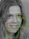
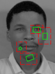
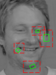
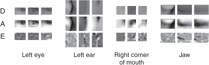
(a) Independent learning by Peng et al. [38]’s method at 20 iterations

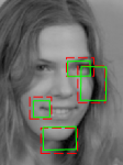
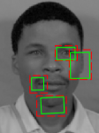
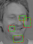
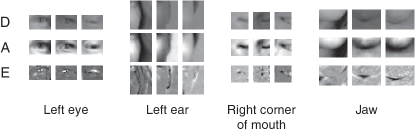
(b) Learning with a known shape constraint at the converged stage.

Figure 5: Part dictionary learning. Parts are initialized at dashed red boxes, and aligned in batch. The solid green boxes denote the obtained domains of the parts. $D$ is a learned part dictionary (images cropped from the obtained domains), and $A+E$ is its best low-rank and sparse decomposition, where $A$ is the low-rank component, and $E$ is the sparse error. The cropped images are normalized in terms of intensity for display convenience.

We learn the part dictionaries from a training gallery of $n$ face images, denoted as $D=[d_{1},d_{2},\ldots,d_{n}]$. Every $k^{\textrm{th}}$ column $d_{k}$ in $D$ represents a stacked vector form of face image in the gallery. Learning part dictionaries is concerned with optimizing the $d$-dimensional $\{\sigma_{k}\in\mathbb{G}\}_{k=1}^{n}$ for holistic deformations and $\{\nu_{k}^{\langle i\rangle}\in\mathbb{G}\}_{k=1}^{n}$, $i=1,\dots,m$, for part deformations, so that after part-based alignment every $i^{\textrm{th}}$ part dictionary, denoted as $D^{\langle i\rangle}=[d_{1}^{\langle i\rangle},d_{2}^{\langle i\rangle},\ldots,d_{n}^{\langle i\rangle}]$ with $d_{k}^{\langle i\rangle}\doteq d_{k}\circ\sigma_{k}\circ\nu_{k}^{\langle i\rangle}$, contains facial parts that have been registered into some canonical form, as shown in Fig. 5b.

We observe that the registered facial parts in each part dictionary correspond to appearance of different subjects at the same facial region. These registered facial parts will ideally resemble each other if nuisances due to inter-subject, illumination, expression, and/or pose variations can be decomposed out. In other words, the part dictionary $D^{\langle i\rangle}$ would be low-rank after decomposing out the aforementioned nuisances, which can be modeled as a sparse error matrix. This sparse and low-rank decomposition was used by Peng et al. [38] to align a batch of linearly correlated images, such as frames in a video sequence or face images of a same subject. Motivated by [38], in this paper, we leverage the very similar low-rank (matrices of part dictionaries without nuisances) and sparsity (error matrices modeling various variations) properties to align and form the part dictionaries. However, if we directly apply techniques of Peng et al. [38] to perform independent part-based alignment, the alignment process often converges to less meaningful solutions as shown in Fig. 5a. The reason is similar to that causing failure of applying the method of Wagner et al. [3] in the case of aligning parts of a probe face to the gallery set, as we explained in Section III. Instead, we constrain part-based alignment for learning part dictionaries by the tree-structured shape model. .

To simplify the notations, we write $\boldsymbol{\sigma}=[\sigma_{1},\ldots,\sigma_{m}]\in\mathbb{R}^{d\times n}$, and combine $\{\nu_{k}^{\langle i\rangle}\}_{k=1,2,\ldots,n}^{i=1,2,\ldots,m}$ into a third-order tensor $\check{\boldsymbol{\nu}}\in\mathbb{R}^{d\times m\times n}$. We define two operators that apply on $\check{\boldsymbol{\nu}}$ as

$$T^{\langle i\rangle}(\check{\boldsymbol{\nu}})=\left[\nu_{1}^{\langle i\rangle},\nu_{2}^{\langle i\rangle},\ldots,\nu_{n}^{\langle i\rangle}\right] \in\mathbb{R}^{d\times n},$$

$$T_{k}(\check{\boldsymbol{\nu}})=\left[\nu_{k}^{\langle 1\rangle},\nu_{k}^{\langle 2\rangle},\ldots,\nu_{k}^{\langle m\rangle}\right] \in\mathbb{R}^{d\times m},$$

where $T^{\langle i\rangle}(\cdot)$ extracts deformation parameters of the $i^{\textrm{th}}$ part of the $n$ face images, and $T_{k}(\cdot)$ extracts those of $m$ facial parts of the $k^{\textrm{th}}$ image. We then write $D^{\langle i\rangle}\doteq D\circ\boldsymbol{\sigma}\circ T^{\langle i\rangle}(\check{\boldsymbol{\nu}})$, where “$\circ$” applies column-wisely. With these definitions our objective for learning part dictionaries can be written as

$$\min_{\underset{i=1,2,\ldots,m}{A^{\langle i\rangle},E^{\langle i\rangle},\check{\boldsymbol{\nu}},\boldsymbol{\sigma}}} \Biggl{\{}\sum_{i=1}^{m}\left(\|A^{\langle i\rangle}\|_{*}+\lambda^{\langle i\rangle}\|E^{\langle i\rangle}\|_{1}\right)$$

$$+\eta\sum_{k=1}^{n}g\left(T_{k}(\check{\boldsymbol{\nu}}),\mathcal{Z}\right)\Biggl{\}}$$

$$\mathrm{s.t.}\quad D\circ\boldsymbol{\sigma}\circ T^{\langle i\rangle}(\check{\boldsymbol{\nu}})=A^{\langle i\rangle}+E^{\langle i\rangle},$$ (20)

where $\|\cdot\|_{*}$ is the nuclear norm, which is a convex surrogate function of matrix rank. As shown by Peng et al. [38], Candès et al. [44], the penalty parameters $\{\lambda^{\langle i\rangle}\}_{i=1}^{m}$ can be set as the reciprocal of the square root of $E^{\langle i\rangle}$’s row number, denoted as $\omega^{\langle i\rangle}$. In this paper, we set $\lambda^{\langle i\rangle}=\hat{\lambda}/\sqrt{\omega^{\langle i\rangle}}$ with the constant $\hat{\lambda}=1$. We accordingly set $\eta=\hat{\eta}\cdot\sum_{i=1}^{m}(\omega^{\langle i\rangle})^{-1/2}$ with $\hat{\eta}$ chosen as $0.02$. To solve (20), we use a similar alternating strategy as in Section III-B. Appendix C gives details of the algorithmic procedure. It requires the initialization of $\check{\boldsymbol{\nu}}$, which can be obtained using the same method as in Session III-B3. Fig. 5b shows example images of learned part dictionaries by solving (20). Compared with independent part-based alignment (example results shown in Fig. 5a), the proposed alignment method with the constraint from a tree-structured model gives much more meaningful results.

V-B Learning the Tree-structured Shape Model Jointly with Part Dictionaries

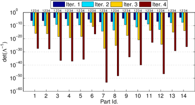
(a) CPA learning with no prior for the tree-structured shape model

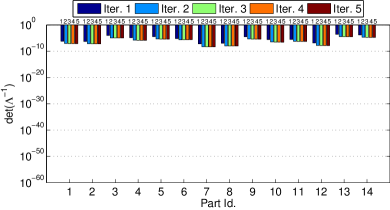
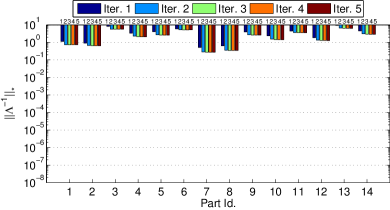
(b) CPA learning with Gaussian-Wishart prior for the tree-structured shape model

Figure 6: Strength of the variances of the Gaussian distributions for the differences of part transformations at different iterations of CPA learning. For a Gaussian distribution, the determinant (left-side figures) and nuclear norm (right-side figures) of its covariance matrix indicate the overall strength of its variances. Larger values indicate better flexibility of the model, and vice versa. In this illustration, we use 60 images from the MUCT dataset [33] to learn the CPA model define in Fig. 1. Both the determinant and nuclear norm are averaged over all the Gaussian distributions attached to the tree edges.

To jointly learn the tree-structured shape model and part dictionaries, it is natural to take $\mathcal{Z}$ in (20) as the additional variables to optimize. To solve this revised problem, one can alternately update part dictionaries using the algorithms in Appendix C, which involves the variables $\{A^{\langle i\rangle}\}_{i=1}^{m}$, $\{E^{\langle i\rangle}\}_{i=1}^{m}$, $\check{\boldsymbol{\nu}}$, and $\boldsymbol{\sigma}$, and estimate $\mathcal{Z}$ by maximum likelihood (ML) estimation, which fits parameters $\{z^{\langle i\rangle}=(\mu^{\langle i\rangle},\Lambda^{\langle i\rangle})\}_{i=1}^{m}$ of Gaussian distributions with the updated $\{T_{k}(\check{\boldsymbol{\nu}})\}_{k=1}^{n}$. Unfortunately, this approach empirically appears to give degenerate solutions corresponding to a “non-elastic” shape model, where the Gaussian distributions modeling the deformation differences of connected nodes in the tree have variances of almost zero magnitude. Fig. 6a illustrates this phenomenon, where we measure the determinant and nuclear norm of the covariance matrices $\{{\Lambda^{\langle i\rangle}}^{-1}\}_{i=1}^{m}$, which are iteratively updated in an alternating optimization process.

To remedy this problem, we consider imposing a prior on $\mathcal{Z}$ to regularize the learning of tree-structured shape model. Denote $h(\mathcal{Z},\Phi)=-\ln p(\mathcal{Z}|\Phi)$ with $\Phi$ as the hyper-parameters. Incorporating $h(\mathcal{Z},\Phi)$ into (20) results in the following new objective for joint learning of $\mathcal{Z}$ and part dictionaries

$$\min_{\underset{i=1,2,\ldots,m}{A^{\langle i\rangle},E^{\langle i\rangle},\check{\boldsymbol{\nu}},\boldsymbol{\sigma},\mathcal{Z}}} \Biggl{\{}\sum_{i=1}^{m}\left(\|A^{\langle i\rangle}\|_{*}+\lambda^{\langle i\rangle}\|E^{\langle i\rangle}\|_{1}\right)$$

$$+\eta \left(\sum_{k=1}^{n}g\left(T_{k}(\check{\boldsymbol{\nu}}),\mathcal{Z}\right)+h(\mathcal{Z},\Phi)\right)\Biggl{\}}$$

$$\mathrm{s.t.}\quad D\circ\boldsymbol{\sigma}\circ T^{\langle i\rangle}(\check{\boldsymbol{\nu}})=A^{\langle i\rangle}+E^{\langle i\rangle}.$$ (21)

Let $\nu_{\delta,k}^{\langle i\rangle}=\nu_{k}^{\langle i\rangle}-\nu_{k}^{\langle j\rangle}$. Based on (5) we have

$$\sum_{k=1}^{n}g\left(T_{k}(\check{\boldsymbol{\nu}}),\mathcal{Z}\right)=-\sum_{i=1}^{m}\ln p(\{\nu_{\delta,k}^{\langle i\rangle}\}_{k=1}^{n}|z^{\langle i\rangle}),$$ (22)

where $z^{\langle i\rangle}=(\mu^{\langle i\rangle},\Lambda^{\langle i\rangle})$, and $\nu_{\delta,k}^{\langle i\rangle}$ is drawn from the Gaussian distribution with mean $\mu^{\langle i\rangle}$ and precision $\Lambda^{\langle i\rangle}$. We impose prior on $\{\mu^{\langle i\rangle},\Lambda^{\langle i\rangle}\}$ using Gaussian-Wishart distribution, which is the conjugate prior of the Gaussian distribution. Denote $\phi^{\langle i\rangle}$ as the parameters of the Gaussian-Wishart prior for $z^{\langle i\rangle}$. We have

$$h(\mathcal{Z},\Phi)=-\sum_{i=1}^{m}\ln p(z^{\langle i\rangle}|\phi^{\langle i\rangle}).$$ (23)

where $\Phi=(\phi^{\langle 1\rangle},\phi^{\langle 2\rangle},\ldots,\phi^{\langle m\rangle})$ is the tuple of the hyper-parameters.

Given $\Phi$, we solve (21) by alternately updating the following two steps:

1. Update $\mathcal{Z}$ by solving $\min_{\mathcal{Z}}\sum_{k=1}^{n}g\left(T_{k}(\check{\boldsymbol{\nu}}),\mathcal{Z}\right)+h(\mathcal{Z},\Phi)$;

2. Update $\{A^{\langle i\rangle}\}_{i=1}^{m},\{E^{\langle i\rangle}\}_{i=1}^{m},\check{\boldsymbol{\nu}},\boldsymbol{\sigma}$ by solving (20).

To update the first step, note that by Bayes’ rule,

$$\sum_{k=1}^{n} g\left(T_{k}(\check{\boldsymbol{\nu}}),\mathcal{Z}\right)+h(\mathcal{Z},\Phi)$$ (24)

$$= -\sum_{i=1}^{m}\left\{\ln p(z^{\langle i\rangle}|\{\nu_{\delta,k}^{\langle i\rangle}\}_{k=1}^{n},\phi^{\langle i\rangle})+\ln p(\{\nu_{\delta,k}^{\langle i\rangle}\}_{k=1}^{n})\right\},$$

where $p(\{\nu_{\delta,k}^{\langle i\rangle}\}_{k=1}^{n})$ does not change with $z^{\langle i\rangle}$, and the terms of the summation have no overlap variables. Thus the above first step can be updated by independently solving the $m$ sub-problems

$$\underset{z^{\langle i\rangle}}{\max}\,p(z^{\langle i\rangle}|\{\nu_{\delta,k}^{\langle i\rangle}\}_{k=1}^{n},\phi^{\langle i\rangle}),$$ (25)

for $i=1,\dots,m$. It is a standard maximum a posterior (MAP) inference for the Gaussian distribution, where the posterior still follows a Gaussian-Wishart distribution, whose parameters are different from those of the prior. The maximum point of a Gaussian-Wishart PDF can be derived in closed form in terms of its parameters. Please refer to Appendix D for details of the Gaussian-Wishart prior and inference problems relevant to it. For the above second step, it is the problem of learning part dictionaries given a fixed $\mathcal{Z}$, which is addressed in the previous subsection.

Now, it comes the problem: how to set hyper-parameters $\{\phi^{\langle i\rangle}\}_{i=1}^{m}$ properly? Since the initialization of $\check{\boldsymbol{\nu}}$ gives rough evidence on how the tree-structured shape model should be, we set $\phi^{\langle i\rangle}$ to be consistent with the ML estimation on $z^{\langle i\rangle}$ with the initial $\check{\boldsymbol{\nu}}$ for $i=1,2,\ldots,m$. Thus, the trained CPA model will not deviate much from its rough estimation. Meanwhile, we also set $\phi^{\langle i\rangle}$ properly to control the prior’s weight, i.e., to make the prior contribute to the MAP estimation as much as $\vartheta n$ training samples, where $\vartheta>0$. Still, please refer to Appendix D for how to set $\phi$ with explicit physical meaning. The above learning procedure for a CPA model is summarized in Algorithm 3.

1:Training images $D$, initial $\check{\boldsymbol{\nu}},\boldsymbol{\sigma}$, and prior weight $\vartheta$

2:learned $\check{\boldsymbol{\nu}},\boldsymbol{\sigma},\mathcal{Z}$

3:$\mathcal{Z}\leftarrow\min_{\mathcal{Z}}\sum_{k=1}^{n}g\left(T_{k}(\check{\boldsymbol{\nu}}),\mathcal{Z}\right)$

4:Set $\Phi$ in consistency to $\mathcal{Z}$ and $\vartheta$

5:while  not converged  do

6:     Update $\{A^{\langle i\rangle}\}_{i=1}^{m},\{E^{\langle i\rangle}\}_{i=1}^{m},\check{\boldsymbol{\nu}},\boldsymbol{\sigma}$ by solving (20).

7:     $\mathcal{Z}\leftarrow\min_{\mathcal{Z}}\sum_{k=1}^{n}g\left(T_{k}(\check{\boldsymbol{\nu}}),\mathcal{Z}\right)+h(\mathcal{Z},\Phi)$

8:end while

Algorithm 3 CPA model learning

The above algorithms for CPA model learning require a careful initialization on $\boldsymbol{\sigma}$ and $\check{\boldsymbol{\nu}}$, which can be done either by detectors [41, 25] or by manual annotations. In particular, for every $k^{\textrm{th}}$ training image, we localize the two eye corners to determine the similarity transform $\sigma_{k}$. We then localize the facial landmarks at the centers of the facial parts, and initialize $\nu_{k}^{\langle i\rangle}$ to satisfy that the $i^{\textrm{th}}$ part has the pre-defined orientation and size relative to the canonical form of the entire face that is determined by $\sigma_{k}$. Although this initialization scheme is very exercisable, but it makes the part transformation differences between linked parts identical for all the $n$ training images. Consequently, we cannot get statistical evidence to learn $\mathcal{Z}$. To overcome this difficulty, we propose a heuristic initialization scheme for learning the CPA model. In particular, we start with the part dictionary learning (20) by setting $\eta=0$, i.e., without any shape constraint, and run it for only a few (here, $5$) iterations of the generalized Gaussian method composed of the repeats of the linearized problem (34) (in the Appendix C). The updated part transformations are used for the actual initialization of the CPA model learning.

Fig. 6b shows the effect of our proposed objective (21) for joint learning of the CPA model, where we investigate the covariance matrices $\{{\Lambda^{\langle i\rangle}}^{-1}\}_{i=1}^{m}$ of the Gaussian distributions obtained in each iteration of our algorithm. Compared with Fig. 6a, the stability of their determinant and nuclear norm values suggests that a better tree-structured shape model is obtained.

Up to now we have assumed that the configuration of the tree, i.e., how the nodes (facial parts) are connected to form the tree, is given. To learn the configuration of a tree, Zhu and Ramanan [25] used Chow and Liu [45] algorithm for the application of facial landmark localization. Chow-Liu algorithm finds the configuration of a Bayesian network that best approximates the joint distribution of all the variables. However, for a node with children, our tree-structured shape model (as well as Zhu and Ramanan [25]’s shape model) assumes the independence between its part transformation and its part transformation differences with its children (refer to Section III-A), which is not an assumption for Chow-Liu algorithm.

Instead, we take the tree configuration that minimizes the objective function for learning the CPA model, which can be reduced to $\sum_{k=1}^{n}g\left(T_{k}(\check{\boldsymbol{\nu}}),\mathcal{Z}\right)+h(\mathcal{Z},\Phi)$ as (24). According to (22) and (23), we can decomposed it into the summation of part-wise scores, where each term associates only with the edge linking one node and its parent. In view of this, we first link the $(m+1)$ nodes (recall the node of “0”) into a complete directed graph, compute the score associating with each of the $(m+1)m$ edges, and take the minimum spanning tree rooted at “0” to be the optimal configuration of the tree.

V-C Learning Mixture of CPA Models

The presented CPA model can be extended as a mixture of CPA models (mCPA) to cope with a larger range of pose and/or expression variations. Each component of the mCPA is parameterized the same as that of a standard CPA model, but it may have a different number of facial parts, since some facial parts may be occluded under pose changes.

For an mCPA model with $c$ components, $\mathcal{I}_{\iota}\subseteq\{1,2,\ldots,m\}$ denotes the index set of available parts for the $\iota^{\textrm{th}}$ component. Correspondingly, we also use $\{D_{\iota}^{\langle i\rangle}\}_{i=1}^{m}$ to denote the part dictionaries and $\mathcal{Z}_{\iota}=\{z_{\iota}^{\langle 1\rangle},z_{\iota}^{\langle 2\rangle},\ldots,z_{\iota}^{\langle m\rangle}\}$ to denote the parameters of tree-structured shape models. If the $\iota^{\textrm{th}}$ component does not has the $i^{\textrm{th}}$ part, i.e. $i\notin\mathcal{I}_{\iota}$, $D_{\iota}^{\langle i\rangle}$ and $z_{\iota}^{\langle i\rangle}$ would just be treated as void notations and would not be used.

Learning an mCPA model is based on the formulation (21) for the standard CPA model learning. The difference is that we consider learning models of the $c$ components altogether, so that the low-rank and sparse properties of corresponding part dictionaries belonging to different components can be overall leveraged, resulting in consistent part dictionaries across the $c$ components. Given $n$ training face images, we write $D_{\iota}$ for the $n_{\iota}$ face images assigned to the $\iota^{\textrm{th}}$ components, $\boldsymbol{\sigma}_{\iota}\in\mathbb{R}^{d\times n_{\iota}}$ for their holistic deformations, and $\check{\boldsymbol{\nu}}{}_{\iota}\in\mathbb{R}^{d\times m\times n_{\iota}}$ for their part deformations. Our objective for learning the mCPA model can be written as

$$\min_{\underset{i=1,2,\ldots,m;\,\iota=1,2,\ldots,c}{A^{\langle i\rangle},E^{\langle i\rangle},\check{\boldsymbol{\nu}}{}_{\iota},\boldsymbol{\sigma}{}_{\iota},\mathcal{Z}{}_{\iota}}}\Biggl{\{}\sum_{i=1}^{m}\left(\|A^{\langle i\rangle}\|_{*}+\lambda^{\langle i\rangle}\|E^{\langle i\rangle}\|_{1}\right)$$ (26)

$$+\eta\sum_{\iota=1}^{c}\left(\sum_{k=1}^{n_{\iota}}g\left(T_{k}(\check{\boldsymbol{\nu}}{}_{\iota}),\mathcal{Z}{}_{\iota}\right)+h(\mathcal{Z}{}_{\iota},\Phi{}_{\iota})\right)\Biggl{\}},$$

s.t.

$$D_{\iota}\circ\boldsymbol{\sigma}_{\iota}\circ T^{\langle i\rangle}(\check{\boldsymbol{\nu}}_{\iota})=A_{\iota}^{\langle i\rangle}+E_{\iota}^{\langle i\rangle}\;\mbox{for }i\in\mathcal{I}_{\iota}.$$

$$A_{\iota}^{\langle i\rangle},E_{\iota}^{\langle i\rangle}\mbox{ are empty matrices for }i\notin\mathcal{I}_{\iota},$$

$$A^{\langle i\rangle}=[A_{1}^{\langle i\rangle},A_{2}^{\langle i\rangle},\ldots,A_{c}^{\langle i\rangle}],$$

$$E^{\langle i\rangle}=[E_{1}^{\langle i\rangle},E_{2}^{\langle i\rangle},\ldots,E_{c}^{\langle i\rangle}].$$

The above objective can be solved similarly as for (21). Namely, we alternately update the part dictionaries and the tree-structured shape models. After solving (26), we have the part dictionaries $D_{\iota}^{\langle i\rangle}\doteq D_{\iota}\circ\boldsymbol{\sigma}_{\iota}\circ T^{\langle i\rangle}(\check{\boldsymbol{\nu}}_{\iota})$ and the shape model parameters $\{\mathcal{Z}_{\iota}\}_{\iota=1}^{c}$.

Given a gallery set, ideally an mCPA model should be learned from face images of this gallery. However, in some cases the gallery does not contain non-frontal/non-neural face images to learn the corresponding component models of the mCPA. To remedy this problem, we first learn an mCPA model using a separate training set that contains face images of all the interested poses and expressions of a few subjects, and then learn the part dictionaries on the gallery set of interest while fixing the learned tree-structured shape model from that separate training set.

With a learned mCPA model, we use the same method as that of the standard CPA model to recognize a probe face, which requires us to select the correct component corresponding to its pose and expression before hand. In a fully automatic face recognition system, we may figure out the pose and expression by off-the-shelf methods, which, we will discuss in Section VI-D.

VI Experiments

In this section, we present experiments to evaluate the proposed CPA method in the context of face recognition across illuminations, poses, and expressions. We used images of frontal face with neutral expression as the gallery, and face images with illumination, pose, and expression variations as the probes. We used the CMU Multi-PIE [32] and MUCT [33] datasets to conduct our experiments. The CMU Multi-PIE dataset contains face images with well controlled illumination, pose, and expression variations, and is thus intensively used for controlled experiments.

Table I: Canonical part locations and sizes for the mCPA component for frontal view and neutral expression in the experiments.

No.	Center location		Relative			Absolute
			w	h		w	h
1	Center of R-eyebrow		0.4	0.2		24	16
2	Center of L-eyebrow		0.4	0.2		24	16
3	Outer corner of R-eye		0.53	0.4		32	32
4	Center of R-eye		0.4	0.2		24	16
5	Inner corner of R-eye		0.58	0.44		35	35
6	Inner corner of L-eye		0.58	0.44		35	35
7	Center of L-eye		0.4	0.2		24	16
8	Outer corner of L-eye		0.53	0.4		32	32
9	R-wing of nose		0.27	0.4		16	32
10	L-wing of nose		0.27	0.4		16	32
11	Apex nasi		0.53	0.28		32	22
12	Philtrum		1.07	0.44		64	35
13	R-corner of mouth		0.32	0.24		19	19
14	L-corner of mouth		0.32	0.24		19	19
15	Mouth center		0.67	0.28		40	22
16	Center of underlip		0.53	0.2		32	16
17	Bottom of jaw		0.53	0.28		32	22
18	R-ear		0.4	0.4		24	32
19	L-ear		0.4	0.4		24	32
20	R-cheek		0.53	0.4		32	32
21	L-cheek		0.53	0.4		32	32

Remark: The relative sizes are in terms of the conventional facial region aligned with the two eyes, i.e., 60$\times$80 window with two outer eye corners at (5,22) and (56,22); and, the absolute sizes are measured in pixels for the part dictionaries.

We designed an mCPA model whose component for frontal view and neutral expression consists of $21$ facial parts of varying sizes. The basic constellation of the $21$ parts is listed in Table I. For the other components, the availability of a part is determined by its visibility. The parameters used for the mCPA learning are set as $\hat{\lambda}=1$, $\hat{\eta}=0.02$, and $\vartheta=0.25$ for all the experiments reported in this section.

With learned mCPA models, we first evaluated our method in Section VI-A in the scenario of face recognition across pose and expression with illumination variation. In particular, we show the advantages of our CPA method over other alternatives, such as the methods of a holistic face alignment followed by a holistic or part-based face recognition. We then demonstrate in Section VI-B the effectiveness of our CPA method when using part-based face recognition strategy. In Section VI-C, we test on face images with synthesized occlusions to demonstrate the robustness of our method. Finally, we compared with the state-of-the-art across-pose face recognition methods in Section VI-D.

For controlled experiments reported in Sections VI-A, VI-B, and VI-C, we initialized face locations by manually annotating eye corner points, and assumed that the pose and expression of each probe face are given. For practical experiments in Section VI-D that conduct fully automatic face recognition across pose, we used off-the-shelf face detector [41] and pose estimator [25] to initialize our method.

VI-A Face Recognition Across Pose and Expression with Different Illumination

Our choice of off-the-shelf methods for face recognition across illumination is based on SRC [26], for which we used multiple gallery images of varying illuminations for each subject. Under this setting, we compare CPA with the following three baseline alternatives.

1. The first one manually aligns probe face images using labeled eye-corner points. After manual alignment, face recognition is conducted in a holistic manner. This alternative method is termed as “manual+holistic”.

2. The second one automatically aligns probe face images using the holistic alignment algorithm of Wagner et al. [3]. After alignment, face recognition is again conducted in a holistic manner. This alternative is termed as “holistic+holistic”. If using SRC [26] as a classifier, this alternative is essentially the same as in [3], which is similar to our CPA method in the way that the gallery is pruned to a subset before being used for recognition. For a fair comparison, we also made the subset consist of $P$ subjects for the alignment algorithm of Wagner et al. [3].

3. The third one also automatically aligns probe face images using the holistic alignment algorithm of Wagner et al. [3]. The same pruning scheme was used as for the second alternative. However, after alignment, a part-based face recognition strategy is used where positions of local parts are pre-defined and fixed relative to the global face. This alternative is termed as “holistic+parted”.

Our CPA method will be occasionally referred to as “mCPA+parted” in accordance with the names of these baselines. The chosen subject number for pruning the gallery was set to $P=20$.

VI-A1 Evaluation on the Multi-PIE Dataset

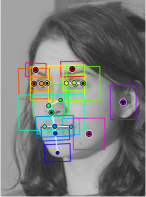
(a) $-\mbox{30}^{\circ}$

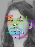
(b) $-\mbox{15}^{\circ}$

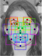
(c) $\mbox{0}^{\circ}$

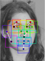
(d) $+\mbox{15}^{\circ}$

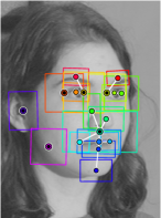
(e) $+\mbox{30}^{\circ}$

Figure 7: The mCPA components fitted to faces with different poses. Refer to the caption of Fig. 3 for explanation.

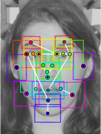
(a) Surprise

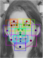
(b) Squint

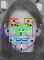
(c) Smile

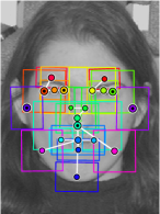
(d) Disgust

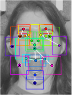
(e) Scream

Figure 8: The mCPA components fitted to faces with non-neutral expressions. Refer to the caption of Fig. 3 for explanation.

The CMU Multi-PIE [32] is the largest publicly available dataset suitable for test of our CPA method. It contains face images of 337 subjects captured over the time span of about 5 months. These face images are organized into 4 sessions according to their capture time. There are 200 ~ 250 subjects present in each session, where every subject is imaged from 15 different viewpoints with the flashlight varying in 18 different directions . Face images in Multi-PIE are with 6 well controlled facial expressions, including the neutral one and 5 non-neutral ones.

In our experiments, we used face images of 7 different illuminations (illumination id: {0, 1, 7, 13, 14, 16, 18}) in the training and gallery sets, and those of a novel illumination (illumination id: 10) in the probe set. We used 9 subjects (subject id: {267, 272, 273, 274, 276, 277, 278, 286, 289}), who appear in all the 2^nd, 3^rd, 4^th sessions, for training of the tree-structured shape model. The 249 subjects that appear in Session 1 (subject id: 1 ~ 249) were used for testing. Their face images in Session 1 constituted the gallery set, and those in the other sessions were the probes. Table IIa gives more specifications on the probes.

For experiments of face recognition across pose on the Multi-PIE dataset, we used the neutral-expression face images of 5 viewpoints of yaw angles at $\mbox{0}^{\circ}$, $\pm\mbox{15}^{\circ}$, and $\pm\mbox{30}^{\circ}$. For those across expression, we used face images of all the 5 available non-neutral expressions under the frontal viewpoint. We built a 10-component mCPA model as shown in Fig. 7 and Fig. 8. Unless otherwise mentioned, these experiment settings were also used in Section VI-B, VI-C, and VI-D.

Table II: Face recognition across pose and expression with different illumination on the first 249 subjects of Multi-PIE dataset. Gallery illuminations: {0, 1, 7, 13, 14, 16, 18}. Probe illumination: 10.

E.0	E.1	E.2	E.3	E.4	E.5
Neutral	Surprise	Squint	Smile	Disgust	Scream
S[234]R1	S2R2	S2R3	S3R2	S3R3	S4R3
Remark: S$a$R$b$ – Recording number $b$ in Session $a$.

(a) Glossary for expressions of the probes.

Align.	Recog.	$-\mbox{30}^{\circ}$		$-\mbox{15}^{\circ}$		$\mbox{0}^{\circ}$		$+\mbox{15}^{\circ}$		$+\mbox{30}^{\circ}$
		13_0		14_0		05_1		05_0		04_1
manual	holistic	8.	03	49.	40	91.	37	58.	03	8.	84
holistic	holistic	13.	45	60.	64	92.	97	80.	52	32.	73
holistic	parted	14.	86	61.	85	94.	78	62.	85	13.	25
mCPA	parted	54.	62	93.	78	99.	60	95.	18	67.	07

(b) Recognition rates (%) for across-pose and neutral-expression (E.0) settings.

Align.	Recog.	E.	1	E.	2	E.	3	E.	4	E.	5
manual	holistic	44.	85	75.	76	64.	78	49.	69	28.	74
holistic	holistic	67.	88	81.	21	68.	55	65.	41	36.	78
holistic	parted	67.	88	81.	21	79.	25	61.	01	43.	10
mCPA	parted	84.	85	93.	33	89.	94	85.	53	58.	62

(c) Recognition rates (%) for across-expression and frontal-pose (05_1) settings

Table IIb reports recognition results of different alternative methods on face images with varying degrees of pose changes. Compared with “manual+holistic”, “holistic+holistic” gives improved performance, which suggests that automatic alignment can improve face registration accuracy and consequently help for face recognition across pose, even in a holistic alignment manner. The performance of “holistic+parted” is unstable, which tells that simple part-based recognition without part alignment is not a feasible approach. Our CPA method significantly outperforms all these baselines. For the 4 non-frontal viewpoints, CPA improves over the best alternative method “holistic+holistic” approximately by 15% ~ 40% in terms of recognition rate.

An interesting observation from Table IIb is that our CPA method can almost perfectly perform face recognition under the across-session setting of Multi-PIE, where probe face images of frontal viewpoint and neutral expression are from Sessions 2, 3 ,4 of Multi-PIE and gallery face images are from Session 1. Under this setting, our method gives 99.60% recognition rate, about 5% higher than that of “holistic+holistic”, i.e., the method in [3]. To the best of our knowledge, this is the best publicly known result under this setting. Note that the challenges of face recognition across sessions are mostly due to appearance change of human faces after a certain period of time, since illumination variation should have ideally been compensated by the multiple images of varying illuminations in the gallery. Nevertheless, our method suggests that by assuming human face as a piece-wise planar surface and using part-wise alignment, the problem of face recognition across sessions can to a large extent be overcome.

Table IIc reports recognition results on frontal-view face images of varying expressions. Comparative performance of different alternative methods is very similar to that reported in Table IIb for face recognition across pose. Our CPA method outperforms the second best “holistic+holistic” method by 12% ~ 21% in terms of recognition rate.

VI-A2 Evaluation on the MUCT Dataset

In practical face recognition scenarios, illumination usually show various levels of strength, and people often present near-neutral expressions. The MUCT dataset is a good simulation of such scenarios, where face images of natural expressions like frowns and minor smiles are captured under frontal lighting of 3 strength levels. We used the first 10 subjects (subject id: 0 ~ 9) of MUCT for training the tree-structured shape model, and the rest 265 for testing. Frontal-view face images (labeled as “a”) were used as gallery, and those of the 4 available non-frontal viewpoints (labeled as “b,c,d,e”) were used as probes.

Table III: Recognition rates (%) for across-pose settings on the MUCT dataset.

Align.	Recog.	Yaw Only				Pitch Only
		$+\mbox{20}^{\circ}$		$+\mbox{38}^{\circ}$		$+\mbox{21}^{\circ}$		$-\mbox{22}^{\circ}$
		b		c		d		e
manual	holistic	99.	17	55.	89	95.	15	99.	58
holistic	holistic	99.	86	93.	20	98.	61	99.	58
holistic	parted	99.	17	69.	21	81.	14	98.	75
mCPA	parted	100		99.	86	99.	86	100

Table III reports recognition results of different alternative methods. Consistent to the results reported in Section VI-A1, our CPA method outperforms all the other 3 alternatives. It in fact performs almost perfectly for all the 4 degrees of pose change.

VI-B Effectiveness of Part-based Recognition in CPA method

The CPA method integrates part alignment with part-based recognition in a cohesive way. Part-based face recognition fuses weaker predictions from individual parts to make a stronger final decision, where a variety of methods can be used for recognition of individual parts. In this section, we investigate the varying discriminative power of individual parts, and also how existing representative face recognition methods perform for part recognition in CPA. We also present experiments to show the efficacy of the proposed pruning scheme in Algorithm 2. These investigations were conducted on the Multi-PIE dataset under the setting of face recognition across pose with different illumination for the gallery and probe (the setting in Section VI-A1 for producing Table IIb).

VI-B1 Part Discriminativeness

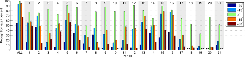
Figure 9: Accuracy of recognizing faces by single parts on Multi-PIE (first 249 subjects). Parts are aligned by CPA, but used individually for recognition. Unavailable parts are referred to as “x”. “ALL” means voting the predicted labels of all the parts.

Fig. 9 reports results obtained by recognizing each of the 21 parts that are jointly aligned by our CPA method. The recognition rates on most of the 21 parts are around 60% ~ 90% for the frontal pose and 40% ~ 80% for the $\pm\mbox{15}^{\circ}$ poses. These results suggest that the discriminativeness of individual parts is good, but not strong enough for a high-accuracy recognition performance. By fusing the predictions from individual parts, a high-accuracy final recognition (“ALL” in Fig. 9) can be achieved for pose change of within $-\mbox{15}^{\circ}$ ~ $+\mbox{15}^{\circ}$ yaw angles. Even for a larger pose change of $\pm\mbox{30}^{\circ}$ yaw angles, our CPA method by fusing predictions from aligned individual parts performs fairly well, while recognition rates for most of individual parts are below 20%. This again demonstrates the efficacy of our proposed CPA method that integrates part-based recognition with part alignment.

VI-B2 Integrated with Different Recognition Methods

Recognition of aligned individual parts in CPA is realized by off-the-shelf face recognition methods. Representatives of these methods include Nearest Subspace (NS) [2], Linear Discriminate Analysis (LDA) [43], and Local Binary Pattern (LBP) [42]. In this section, we investigate how these different choices of recognition methods perform when integrated into our CPA method. Here we compared the CPA method (“mCPA+parted”) with only “holistic+holistic”.

For LDA, we learned its projection matrix after pruning candidate subjects and aligning gallery images, both of which are necessary steps for “holistic+holistic” and our CPA method. For LBP, we also extracted LBP features in the same stage, i.e., after the preparation of aligned gallery subsets. All the experimental settings were the same as those used in preceding sections, expect replacing the previously used SRC with NS, LDA, or LBP. Considering the promise of LBP for one-shot face recognition where only a single image per subject is available in gallery, we also conducted experiments under this one-shot setting, where probe and gallery face images are of the same illumination. Table IVa summarizes the illumination settings of experiments reported in this section.

Table IV: Integrated with different recognition methods on Multi-PIE (first 249 subjects)

Strategy	Gallery illumi.	Probe illumi.
DI: Different illum.	0, 1, 7, 13, 14, 16, 18	10
SI: Same illum.	7	7

(a) Illumination settings

Recog.	Align.	$-\mbox{30}^{\circ}$		$-\mbox{15}^{\circ}$		$\mbox{0}^{\circ}$		$+\mbox{15}^{\circ}$		$+\mbox{30}^{\circ}$
		13_0		14_0		05_1		05_0		04_1
NS	holistic	8.	84	44.	38	76.	31	60.	44	20.	68
(DI)	mCPA	43.	98	85.	94	98.	19	88.	76	65.	26
LDA	holistic	9.	64	42.	57	84.	94	63.	45	16.	67
(DI)	mCPA	26.	51	73.	90	98.	80	77.	31	28.	57
LBP	holistic	34.	34	79.	52	95.	18	88.	35	39.	76
(DI)	mCPA	59.	44	86.	95	97.	39	87.	55	65.	06
LBP	holistic	57.	03	92.	77	97.	39	92.	97	60.	44
(SI)	mCPA	83.	53	96.	99	98.	80	95.	38	76.	91

(b) Recognition rates for across-pose and neutral-expression settings

Recognition rates of CPA with integration of different methods are reported in Table IVb. Table IVb tells that with any choice of NS, LDA, or LBP, our proposed CPA for part-based alignment is superior to holistic face alignment. This confirms that our proposed CPA helps face recognition by effectively aligning individual facial parts.

VI-B3 Pruning Efficacy

Pruning scheme in Algorithm 2 certainly leads to more efficient algorithm. In this section, we are interested in investigating how it impacts the recognition performance. To this end, we modified Algorithm 2 by simply removing the pruning scheme, i.e., setting $P$ to the subject number in the gallery. Bottom half of Table V lists recognition rates of the non-pruning CPA method together with their difference with those of the original CPA. For the non-frontal poses, noticeable performance drops occur when the pruning scheme is removed from CPA. Top half of Table V gives more evidence on the impact of the pruning scheme. Taking the non-pruning version as the baseline, we find that, for the non-frontal poses, the original CPA method corrects one time more recognition errors than it introduces, where “correcting” a recognition error means correctly recognizing an image that is falsely recognized by the baseline, and “introducing” means the opposite. Experimental results reported in Table V were obtained by using SRC for part recognition. All other settings were the same as those used in preceding sections.

Table V: Impact of the pruning scheme on CPA (first 249 subjects of Multi-PIE): the standard CPA is compared with the CPA without pruning scheme (the baseline). Top half: “Corrected” errors are those occurred for the baseline but not for the standard CPA, and the “introduced” errors are the opposite. Bottom half: $\Delta\mbox{RR}=\mbox{(Standard CPA's RR)}-\mbox{(Baseline's RR)}$.

Errors …	Cnt.	$-\mbox{30}^{\circ}$	$-\mbox{15}^{\circ}$	$\mbox{0}^{\circ}$	$+\mbox{15}^{\circ}$	$+\mbox{30}^{\circ}$
by pruning	type	13_0	14_0	05_1	05_0	04_1
Corrected	Num.	77	26	0	26	78
	%	15.46	5.22	0.00	4.22	15.66
Introduced	Num.	33	14	1	14	39
	%	6.63	2.81	0.20	2.01	7.83
RR – no pruning %		45.78	91.37	99.80	92.97	59.24
$\Delta$RR with orig. %		8.84	2.41	$-$0.20	2.21	7.83
Remarks: RR – recognition rate; orig. – pruning with $P=20$.

VI-C Recognition with Synthetic Random Block Occlusion

10% 20% 30% 40% 50% 60%

Figure 10: Images with synthetic block occlusions of different size. The percents below the images indicates the occlusion ratio with respect to the regions enclosed with dashed lines.

We report experiments in this section to demonstrate the robustness of CPA against partial occlusion. As shown in Fig. 10, we synthesized partially occluded probe face images by adding block occlusion at random positions of a probe face. The size of occluded blocks varied from 10% to 60% of the holistic face. Experiment settings were set the same as in Section VI-A1. The method [3], i.e. “holistic+holistic”, was taken as the baseline.

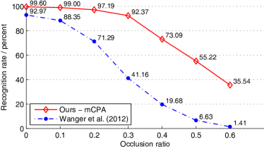
(a) Recognition rates at different occlusion levels for the frontal-pose and neutral-expression setting

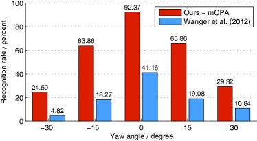
(b) Recognition rates for across-pose and neural-expression settings with the occlusion ratio of 30%

Figure 11: Recognition rates on Multi-PIE (first 249 subjects) when synthetic random block occlusions are present

Fig. 11a reports recognition rates on frontal-view face images at different occlusion ratios, and Fig. 11b reports those of varying viewpoints at the occlusion ratio of 30%. Compared with [3], Fig. 11a and Fig. 11b show that our CPA method is more robust against partial occlusion. When a small portion (10%) of face images is occluded, recognition rate of [3] drops below 90%. In contrast, recognition rates of CPA remain above 90% when the occlusion ratios increase from 0% to 30%. For the 30% occlusion ratio, recognition rate of CPA is more than 45% higher than that of [3] for pose change of within $\pm 15^{\circ}$.

VI-D Comparison with the State-of-the-art

In this section, we used the Multi-PIE dataset to compare CPA with the state-of-the-art Morphable Displacement Field (MDF) method [34] for face recognition across pose. MDF achieves good performance by learning an MDF model from a large number of 3D face shapes, while training of CPA only requires 2D face images of a few subjects.

Like our CPA method, MDF can also be equipped with different features and classifiers for recognition. In order fairly compare the two methods, in this paper, we used the same LDA classifier for both the two methods . While LDA models were learned from pruned gallery in the CPA method, a single LDA model was learned from the entire gallery set in advance for the MDF method, as it does not prune gallery during recognition.

We compare the CPA and MDF methods using probe face images that are under different pose and illumination conditions from those of gallery images. The experiment settings were largely the same as those of face recognition across pose with different illumination used in Session VI-A1, except that:

1. In order to be consistent with the experimental protocol in the work of Li et al. [34], we used the last 137 subjects instead of the first 229 ones in Multi-PIE for testing. More specifically, for each subject, face images in the session where he/she first appears were included in the gallery set, and those in the other sessions were in the probe set.

2. We learned the tree-structured shape model in CPA using face images of 9 other subjects (subject id: {038, 040, 041, 042, 043, 044, 046, 047, 048}), who appear in all the four sessions of Multi-PIE.

3. We set $P=10$ for the pruning scheme used in Algorithm 2.

Table VIa reports recognition rates of CPA and MDF on neutral-expression face images of varying degrees of pose change, where both fully automatic and semi-automatic (manual initialization with known pose) experiments are reported. For the case of semi-automatic experiments using LDA as the classifier, our CPA method outperforms MDF when the degrees of pose change are within $\pm\mbox{15}^{\circ}$. When the degrees of pose change increase to $\pm\mbox{30}^{\circ}$, CPA performs worse than MDF. The performance inconsistency between smaller and larger degrees of pose change is in fact determined by the algorithm nature of the two methods. CPA is based on 2D similarity transform of individual facial parts, whose training only requires face images of a few subjects, while a large number of 3D face shapes are necessary for learning an MDF model. By learning more generic knowledge of 3D face shapes, MDF is able to better cope with face recognition across a larger degree of pose change. However, for the range between $-15$ and $+15$ degrees, which are more often encountered in practical scenarios such as access control, and face recognition in which is also more reliable, CPA gives more accurate recognition results than MDF does. In addition, our CPA method with SRC gives similarly better results in this range of pose change.

We realize a fully automatic CPA method by initializing our algorithm using Viola and Jones [41]’s face detector, followed by a coarse and holistic alignment using the method of Wagner et al. [3]. For knowledge of face pose used in the mCPA model, we consider two situations where poses of probe faces are either known in advance or estimated by Zhu and Ramanan [25]’s method. The accuracy rate of Zhu et al.’s pose estimator is 96.56% under our experiment settings .

Table VIb reports recognition results of fully automatic CPA. Fully automatic CPA (the last two rows) performs comparably with the semi-automatic one (the first row) when pose changes of probe face images are within $\pm\mbox{15}^{\circ}$. Note that the fully automatic alignment works from coarse to fine granularity, say, sequentially uses Viola and Jones [41]’s face detector, the method of Wagner et al. [3] for a holistic alignment, and part-based alignment by CPA. The experimental results show that this coarse-to-fine strategy works well for reasonable degrees of pose change (e.g., within $\pm\mbox{15}^{\circ}$). For larger degrees of pose change, performance of holistic alignment by [3] drops. Consequently, our method loses the chance of correcting its alignment failure. In addition, the last two rows of Table VIb also tells that the mCPA model performs equally well when poses of probe faces are either given or automatically estimated. This confirms the effectiveness of our proposed method for automatic part-based face alignment.

Table VI: Face recognition across pose and expression with different illumination on the last 137 subjects of Multi-PIE. Gallery illuminations: {0, 1, 7, 13, 14, 16, 18}. Probe illumination: 10.

Alignment	$-\mbox{30}^{\circ}$	$-\mbox{15}^{\circ}$	$\mbox{0}^{\circ}$	$+\mbox{15}^{\circ}$	$+\mbox{30}^{\circ}$
	13_0	14_0	05_1	05_0	04_1
MDF	68.71	82.21	/	80.37	74.85
mCPA	38.65	85.28	98.77	86.50	47.24

(a) Recognition rates of MDF and CPA when integrated with LDA. Initialization is manually done by fitting eye-corner annotations, and pose is known in advance.

Initial-	Pose	$-\mbox{30}^{\circ}$	$-\mbox{15}^{\circ}$	$\mbox{0}^{\circ}$	$+\mbox{15}^{\circ}$	$+\mbox{30}^{\circ}$
ization		13_0	14_0	05_1	05_0	04_1
manual	known	53.37	87.12	98.16	87.73	76.07
auto*	known	32.52	82.82	99.39	94.48	57.06
auto*	auto**	33.13	80.98	99.39	94.48	57.06
* face detector followed by holistic alignment; ** pose estimator.

(b) Recognition rates of the CPA method integrated with SRC for different initialization and pose estimation schemes.

VII Conclusion

In this paper we propose a method termed CPA for across-pose and -expression face recognition, which can be benefited by pixel-wisely accurate alignment. The CPA model consists of appearance evidence of each part and a tree-structured shape model for constraining part deformation, both of which can be automatically learned from training images. To align a probe image, we fit its parts to the appearance evidence with consideration of constraint from the learned tree-structured shape model. This objective is formulated as a norm minimization problem regularized by the graph likelihoods, which can be efficiently solved by an alternating optimization method. CPA can easily incorporate many existing face recognition method for part-based recognition. Intensive experiments show the efficacy of CPA in handling illumination, pose, and/or expression changes when integrated with an recognition method robust to illumination changes. In further research, we are interested in applying applying/adapting CPA to other computer vision applications.

Appendix A Linear System in (17)

Let $Q=[q_{1},q_{2},\ldots,q_{m}]\in\mathbb{R}^{d\times m}$, (17) is the same as the linear equation array:

$$G^{\langle i\rangle}\Delta\nu^{\langle i\rangle}+\eta\left(\dfrac{\partial g(\boldsymbol{\nu}+\Delta\boldsymbol{\nu},\mathcal{Z})}{\partial\Delta\nu^{\langle i\rangle}}\right)^{T}=q_{i},$$ (27)

for $i=1,2,\ldots,m$, which can be written in a more standard form

$$\begin{pmatrix}W_{11}&W_{12}&\cdots&W_{1m}\\ W_{21}&W_{22}&\cdots&W_{2m}\\ \vdots&\vdots&\ddots&\vdots\\ W_{m1}&W_{m2}&\cdots&W_{mm}\end{pmatrix}\begin{pmatrix}\Delta\nu^{\langle 1\rangle}\\ \Delta\nu^{\langle 2\rangle}\\ \vdots\\ \Delta\nu^{\langle m\rangle}\end{pmatrix}=\begin{pmatrix}c_{1}\\ c_{2}\\ \vdots\\ c_{m}\end{pmatrix},$$ (28)

where $c_{i}\in\mathbb{R}^{d}$ is a column vector, and $W_{ij}\in\mathbb{R}^{d\times d}$. Recall that $\mathcal{E}$ is the edge set of the tree-structured model. In particular, if $i$ is the parent of $j$, it holds $(i,j)\in\mathcal{E}$. Now, we can find that

$$c_{i}=q_{i}+\eta\left(\Lambda^{\langle i\rangle}(\mu^{\langle i\rangle}-\nu_{\delta}^{\langle i\rangle})-\sum_{j\in\{(i,j)\in\mathcal{E}\}}\Lambda^{\langle j\rangle}(\mu^{\langle j\rangle}-\nu_{\delta}^{\langle j\rangle})\right),$$

for $i=1,2,\ldots,m$, and

$$W_{ij}=\begin{cases}G^{\langle i\rangle}+\eta\sum_{l\in\{i\}\cup\{l:(i,l)\in\mathcal{E}\}}\Lambda^{\langle l\rangle},&j=i,\\ -\eta\Lambda^{\langle j\rangle},&(i,j)\in\mathcal{E},\\ -\eta\Lambda^{\langle i\rangle},&(j,i)\in\mathcal{E},\\ \mathbf{0},&\mbox{otherwise},\end{cases}$$

for for $i,j=1,2,\ldots,m$.

Appendix B Solving Transformations in (18) with Fixed Parts

$\mathbb{G}$ is the 2-D similarity group parametrized in $\mathbb{R}^{d}$ ($d=4$) as it is defined in (1). Given initial values on $\sigma\in\mathbb{G}$ and $\{\nu^{\langle i\rangle}\}_{i=1}^{m}\in\mathbb{G}$, (18) seeks the minimum of $g\left(\boldsymbol{\nu},\mathcal{Z}\right)$ while keeping the value of $\sigma\circ\nu^{\langle i\rangle}$ unchanged. Let $\boldsymbol{\nu}=[\nu^{\langle 1\rangle},\nu^{\langle 2\rangle},\ldots,\nu^{\langle m\rangle}]\in\mathbb{R}^{d\times m}$, and $\Delta\boldsymbol{\nu}=[\Delta\nu^{\langle 1\rangle},\Delta\nu^{\langle 2\rangle},\ldots,\Delta\nu^{\langle m\rangle}]\in\mathbb{R}^{d\times m}$. We reformulate (18) as

$$\min_{\Delta\boldsymbol{\nu},\Delta\sigma}g\left(\boldsymbol{\nu}+\Delta\mbox{$\boldsymbol{\nu}$},\mathcal{Z}\right),$$ (29)

$$\mathrm{s.t.}\quad(\sigma+\Delta\mbox{$\sigma$})\circ(\nu^{\langle i\rangle}+\Delta\mbox{$\nu$}^{\langle i\rangle})=\sigma\circ\nu^{\langle i\rangle}.$$ (30)

After optimizing it, $\sigma$ is updated to $\sigma+\Delta\sigma$, and $\boldsymbol{\nu}$ is updated to $\boldsymbol{\nu}+\Delta\boldsymbol{\nu}$.

Let

$$\mbox{$\nu$}^{\langle i\rangle} \,=\; (s^{\langle i\rangle},\theta^{\langle i\rangle},t_{u}^{\langle i\rangle},t_{v}^{\langle i\rangle}),$$

$$\Delta\sigma \,=\; (\delta s^{*},\delta\theta^{*},\delta t_{u}^{*},\delta t_{v}^{*}),$$

where $s^{\cdot},\theta^{\cdot},t_{u}^{\cdot},t_{v}^{\cdot}$ (“$\cdot$” for “$\langle i\rangle$” and “$*$”) respectively denote the scale, rotation, horizontal translation, and vertical translation of a 2-D similarity transformation. (30) is equivalent to

$$\Delta\mbox{$\nu$}^{\langle i\rangle}=\left(\begin{array}[]{c}-\delta s^{*}\\ -\delta\theta^{*}\\ -t_{u}^{\langle i\rangle}+f_{u}^{*}+f_{u}^{\langle i\rangle}\\ -t_{v}^{\langle i\rangle}+f_{v}^{*}+f_{v}^{\langle i\rangle}\end{array}\right),$$ (31)

where,

$$f_{u}^{*}= \frac{(t_{u}^{*},t_{v}^{*})}{\exp(\delta s^{*}+s^{*})}\left(\begin{array}[]{c}\cos(\delta\theta^{*}+\theta^{*})\\ \sin(\delta\theta^{*}+\theta^{*})\end{array}\right),$$

$$f_{v}^{*}= \frac{(t_{v}^{*},-t_{u}^{*})}{\exp(\delta s^{*}+s^{*})}\left(\begin{array}[]{c}\cos(\delta\theta^{*}+\theta^{*})\\ \sin(\delta\theta^{*}+\theta^{*})\end{array}\right),$$

and,

$$f_{u}^{\langle i\rangle}= \frac{(t_{u}^{\langle i\rangle},t_{v}^{\langle i\rangle})}{\exp(\delta s^{*})}\left(\begin{array}[]{c}\cos\delta\theta^{*}\\ \sin\delta\theta^{*}\end{array}\right),$$

$$f_{v}^{\langle i\rangle}= \frac{(t_{v}^{\langle i\rangle},-t_{u}^{\langle i\rangle})}{\exp(\delta s^{*})}\left(\begin{array}[]{c}\cos\delta\theta^{*}\\ \sin\delta\theta^{*}\end{array}\right).$$

Substituting (31) into the objective function in (29), we obtain the unconstrained equivalence of the original problem, say, $\min_{\Delta\sigma}g\left(\boldsymbol{\nu}+\Delta\mbox{$\boldsymbol{\nu}$},\mathcal{Z}\right)$, where $\Delta\boldsymbol{\nu}$ is expended as (31). We solve this problem by gradient descent. Now, we need to find $g\left(\boldsymbol{\nu}+\Delta\mbox{$\boldsymbol{\nu}$},\mathcal{Z}\right)$’s gradient in $\Delta\sigma$.

Recall that $\mathcal{E}$ is the tree edge set. For $i=1,2,\ldots,m$, let $j$ satisfies $(j,i)\in\mathcal{E}$ ($j$ is the parent of $i$), and

$$\varphi^{\langle i\rangle}=\left((\mbox{$\nu$}^{\langle i\rangle}+\Delta\mbox{$\nu$}^{\langle i\rangle})-(\mbox{$\nu$}^{\langle i\rangle}+\Delta\mbox{$\nu$}^{\langle j\rangle})-\mu^{\langle i\rangle}\right),$$

We then have

$$g\left(\boldsymbol{\nu}+\Delta\mbox{$\boldsymbol{\nu}$},\mathcal{Z}\right)=\frac{1}{2}\sum_{i=1}^{m}{\varphi^{\langle i\rangle}}^{T}\Lambda^{\langle i\rangle}\varphi^{\langle i\rangle}+b,$$ (32)

and,

$$\nabla_{(\Delta\sigma)}g\left(\boldsymbol{\nu}+\Delta\mbox{$\boldsymbol{\nu}$},\mathcal{Z}\right)=\sum_{i=1}^{m}{\varphi^{\langle i\rangle}}^{T}\Lambda^{\langle i\rangle}\frac{\partial\varphi^{\langle i\rangle}}{\partial(\Delta\sigma)}.$$ (33)

For $i$ satisfying $(0,i)\in\mathcal{E}$ ($i$ is directly linked with the root), it holds

$$\varphi^{\langle i\rangle}=\left(\begin{array}[]{c}s^{\langle i\rangle}-\delta s^{*}\\ \theta^{\langle i\rangle}-\delta\theta^{*}\\ f_{u}^{\langle i\rangle}-f_{u}^{*}\\ f_{v}^{\langle i\rangle}-f_{v}^{*}\end{array}\right)-\mu^{\langle i\rangle},$$

$$\frac{\partial\varphi^{\langle i\rangle}}{\partial(\Delta\sigma)}=$$

$$\;\left(\begin{array}[]{cccc}-1&0&0&0\\ 0&-1&0&0\\ f_{u}^{*}-f_{u}^{\langle i\rangle}&f_{v}^{\langle i\rangle}-f_{v}^{*}&-\frac{\cos(\delta\theta^{*}+\theta^{*})}{\exp(\delta s^{*}+s^{*})}&-\frac{\sin(\delta\theta^{*}+\theta^{*})}{\exp(\delta s^{*}+s^{*})}\\ f_{v}^{*}-f_{v}^{\langle i\rangle}&f_{u}^{*}-f_{u}^{\langle i\rangle}&\frac{\sin(\delta\theta^{*}+\theta^{*})}{\exp(\delta s^{*}+s^{*})}&-\frac{\cos(\delta\theta^{*}+\theta^{*})}{\exp(\delta s^{*}+s^{*})}\end{array}\right).$$

For $i$ satisfying $(j,i)\in\mathcal{E},j\neq 0$ ($i$ is not directly linked with the root), it holds

$$\varphi^{\langle i\rangle}=\left(\begin{array}[]{c}s^{\langle i\rangle}-s^{\langle j\rangle}\\ \theta^{\langle i\rangle}-\theta^{\langle j\rangle}\\ f_{u}^{\langle i\rangle}-f_{u}^{\langle j\rangle}\\ f_{v}^{\langle i\rangle}-f_{v}^{\langle j\rangle}\end{array}\right)-\mu^{\langle i\rangle},$$

$$\frac{\partial\varphi^{\langle i\rangle}}{\partial(\Delta\sigma)}=\left(\begin{array}[]{cccc}0&0&0&0\\ 0&0&0&0\\ f_{u}^{\langle j\rangle}-f_{u}^{\langle i\rangle}&f_{v}^{\langle i\rangle}-f_{v}^{\langle j\rangle}&0&0\\ f_{v}^{\langle j\rangle}-f_{v}^{\langle i\rangle}&f_{u}^{\langle j\rangle}-f_{u}^{\langle i\rangle}&0&0\end{array}\right).$$

Appendix C Solution to (21)

We solve (21) by the alternately conducting the following two steps:

1. Fix $\boldsymbol{\sigma}$ and solve $\check{\boldsymbol{\nu}},\{A^{\langle i\rangle}\}_{i=1}^{m},\{E^{\langle i\rangle}\}_{i=1}^{m}$.

2. Fix $\{A^{\langle i\rangle}\}_{i=1}^{m},\{E^{\langle i\rangle}\}_{i=1}^{m}$ and solve $\boldsymbol{\sigma},\check{\boldsymbol{\nu}}$.

Step 1: Given fixed $\boldsymbol{\sigma}$, we update $\check{\boldsymbol{\nu}}$ by a generalization of the Gauss-Newton method. To be specific, for a linear update from $\check{\boldsymbol{\nu}}$ to $\check{\boldsymbol{\nu}}+\Delta\check{\boldsymbol{\nu}}$ ($\Delta\check{\boldsymbol{\nu}}\in\mathbb{R}^{d\times m\times n}$), we approximate the equality constraint in (21) by its first-order Taylor expansion at $T^{\langle i\rangle}(\check{\boldsymbol{\nu}})$, i.e., $D\circ\boldsymbol{\sigma}\circ T^{\langle i\rangle}(\check{\boldsymbol{\nu}})\approx D\circ\boldsymbol{\sigma}\circ T^{\langle i\rangle}(\check{\boldsymbol{\nu}})+\sum_{k=1}^{n}J_{k}^{\langle i\rangle}T^{\langle i\rangle}(\Delta\check{\boldsymbol{\nu}})\epsilon_{k}\epsilon_{k}^{T}$, where $J_{k}^{\langle i\rangle}\doteq\partial(d_{k}\circ\sigma_{k}\circ\nu_{k}^{\langle i\rangle})/\partial\nu_{k}^{\langle i\rangle}$ is the Jacobian w.r.t. $\nu_{k}^{\langle i\rangle}$, and $\{\epsilon_{k}\}_{k=1}^{n}$ denotes the standard basis of $\mathbb{R}^{n}$. The above linearization leads to the following problem to optimize $\{A^{\langle i\rangle}\}_{i=1}^{m},\{E^{\langle i\rangle}\}_{i=1}^{m},\Delta\check{\boldsymbol{\nu}}$

$$\min_{\underset{i=1,2,\ldots,m}{A^{\langle i\rangle},E^{\langle i\rangle},\Delta\check{\boldsymbol{\nu}}}} \Biggl{\{}\sum_{i=1}^{m}\left(\|A^{\langle i\rangle}\|_{*}+\lambda^{\langle i\rangle}\|E^{\langle i\rangle}\|_{1}\right)$$

$$+\eta\sum_{k=1}^{n}g\left(T_{k}(\check{\boldsymbol{\nu}}+\Delta\check{\boldsymbol{\nu}}),\mathcal{Z}\right)\Biggl{\}}$$ (34)

$$\mathrm{s.t.}\quad D\circ\boldsymbol{\sigma}\circ T^{\langle i\rangle}(\check{\boldsymbol{\nu}})+\sum_{k=1}^{n}J_{k}^{\langle i\rangle}T^{\langle i\rangle}(\Delta\check{\boldsymbol{\nu}})\epsilon_{k}\epsilon_{k}^{T}=A^{\langle i\rangle}+E^{\langle i\rangle}.$$

We repeatedly solve (34) to update $\check{\boldsymbol{\nu}}$, until it converges to a local minimum, which gives the solution to the original problem(21) .

We solve the convex problem (34) by adapting the ALM. Let

$$h( A^{\langle i\rangle},E^{\langle i\rangle},T^{\langle i\rangle}(\Delta\check{\boldsymbol{\nu}}))=$$

$$D\circ\boldsymbol{\sigma}\circ T^{\langle i\rangle}(\check{\boldsymbol{\nu}})+\sum_{k=1}^{n}J_{k}^{\langle i\rangle}T^{\langle i\rangle}(\Delta\check{\boldsymbol{\nu}})\epsilon_{k}\epsilon_{k}^{T}-A^{\langle i\rangle}-E^{\langle i\rangle}.$$

The augmented Lagrange function is written as

$$L_{\beta}(\{A^{\langle i\rangle}\}_{i=1}^{m},\{E^{\langle i\rangle}\}_{i=1}^{m},\Delta\check{\boldsymbol{\nu}},\{\Gamma^{\langle i\rangle}\}_{i=1}^{m})=$$ (35)

$$\sum_{i}^{m}\biggl{\{}\|A^{\langle i\rangle}\|_{*}+\lambda^{\langle i\rangle}\|E^{\langle i\rangle}\|_{1}+\left\langle\Gamma^{\langle i\rangle},h(A^{\langle i\rangle},E^{\langle i\rangle},T^{\langle i\rangle}(\Delta\check{\boldsymbol{\nu}}))\right\rangle$$

$$+\frac{\mu}{2}\left\|h(A^{\langle i\rangle},E^{\langle i\rangle},T^{\langle i\rangle}(\Delta\check{\boldsymbol{\nu}}))\right\|_{F}^{2}\biggl{\}}+\sum_{k=1}^{n}g\left(T_{k}(\check{\boldsymbol{\nu}}+\Delta\check{\boldsymbol{\nu}}),\mathcal{Z}\right),$$

where $\{\Gamma^{\langle i\rangle}\}_{i=1}^{m}$ are the Lagrange multiplier matrices, and the matrix inner product $\langle\cdot,\cdot\rangle$ is defined as $\langle A,B\rangle=\operatorname{trace}(A^{T}B)$. Given initial $\{\Gamma^{\langle i\rangle}\}_{i=1}^{m}$, ALM iteratively and alternately updates $\{A^{\langle i\rangle}\}_{i=1}^{m},\{E^{\langle i\rangle}\}_{i=1}^{m},\Delta\check{\boldsymbol{\nu}}$, and $\{\Gamma^{\langle i\rangle}\}_{i=1}^{m}$ by

1. $\{A^{\langle i\rangle}\}_{i=1}^{m},\{E^{\langle i\rangle}\}_{i=1}^{m},\Delta\check{\boldsymbol{\nu}}\leftarrow$

   $$\mbox{}\underset{\underset{i=1,2,\ldots,m}{A^{\langle i\rangle},E^{\langle i\rangle},\Delta\check{\boldsymbol{\nu}}}}{\arg\min}\,L_{\beta}(\{A^{\langle i\rangle}\}_{i=1}^{m},\{E^{\langle i\rangle}\}_{i=1}^{m},\Delta\check{\boldsymbol{\nu}},\{\Gamma^{\langle i\rangle}\}_{i=1}^{m});$$ (36)

2. $\Gamma^{\langle i\rangle}\leftarrow\Gamma^{\langle i\rangle}+\beta_{l}\cdot h(A^{\langle i\rangle},E^{\langle i\rangle},T^{\langle i\rangle}(\Delta\check{\boldsymbol{\nu}}))$,
   for $i=1,2,\ldots,m;$

where $l$ is the iteration number, and $\{\beta_{l}\}_{l=1,2,\ldots}$ is an sequence increasing to sufficient large.

Directly solving (36) w.r.t. all the unknown variables is still a difficult problem. Instead, we alternately update them in three groups, i.e., $\{A^{\langle i\rangle}\}_{i=1}^{m}$, $\{E^{\langle i\rangle}\}_{i=1}^{m}$, and $\Delta\check{\boldsymbol{\nu}}$, so that each subproblem associated with any single group of variables has a closed form solution. More specifically, for $i=1,2,\ldots,m$, we update $A^{\langle i\rangle}$ and $E^{\langle i\rangle}$ sequentially by

$$R^{\langle i\rangle} \leftarrow D\circ\boldsymbol{\sigma}\circ T^{\langle i\rangle}(\check{\boldsymbol{\nu}})+(1/\beta_{l})\Gamma^{\langle i\rangle},$$

$$(\hat{U}, \hat{\Sigma},\hat{V})\leftarrow\operatorname{svd}\left(R^{\langle i\rangle}+\sum_{k}^{n}J_{k}^{\langle i\rangle}T^{\langle i\rangle}(\Delta\check{\boldsymbol{\nu}})\epsilon_{k}\epsilon_{k}^{T}-E^{\langle i\rangle}\right),$$

$$A^{\langle i\rangle} \leftarrow\hat{U}\mathcal{S}_{1/\beta_{l}}(\hat{\Sigma}){\hat{V}}^{T},$$

$$E^{\langle i\rangle} \leftarrow\mathcal{S}_{\lambda^{\langle i\rangle}/\beta_{l}}\left(R^{\langle i\rangle}+\sum_{k}^{n}J_{k}^{\langle i\rangle}T^{\langle i\rangle}(\Delta\check{\boldsymbol{\nu}})\epsilon_{k}\epsilon_{k}^{T}-A^{\langle i\rangle}\right),$$

where $R^{\langle i\rangle}$ is an auxiliary variable used for notation convenience, $\mathcal{S}_{\alpha}(\cdot)$ is the soft-thresholding function defined in (14). Then, for $k=1,2,\ldots,n$, we find the optimum $T_{k}(\Delta\check{\boldsymbol{\nu}})$ by solving

$$\mathbf{0}= \frac{\partial L_{\mu}(\{A^{\langle i\rangle}\}_{i=1}^{m},\{E^{\langle i\rangle}\}_{i=1}^{m},\Delta\check{\boldsymbol{\nu}})}{\partial\Delta\nu_{k}^{\langle i\rangle}}$$ (37)

$$= \beta_{l}\left((R^{\langle i\rangle}-A^{\langle i\rangle}-E^{\langle i\rangle})\epsilon_{k}+J_{k}^{\langle i\rangle}\Delta\nu_{k}^{\langle i\rangle}\right){J_{k}^{\langle i\rangle}}$$

$$+\eta\frac{\partial g(T_{k}(\check{\boldsymbol{\nu}}),\mathcal{Z})}{\partial\Delta\nu_{k}^{\langle i\rangle}},$$

for $i=1,2,\ldots,m$. The $m$ equations forms a sparse linear system of the form in (17) (expended form in Appendix A), whose parameters are $\{G^{\langle i\rangle}\}_{i=1}^{m}$ and $Q$. Here, $G^{\langle i\rangle}=\beta_{l}{J_{k}^{\langle i\rangle}}^{T}J_{k}^{\langle i\rangle}$, the $i^{\textrm{th}}$ column of $Q$ is $\beta_{l}(A^{\langle i\rangle}+E^{\langle i\rangle}-R^{\langle i\rangle})\epsilon_{k}$. Still, we use the inexact scheme for ALM, in which $\{A^{\langle i\rangle}\}_{i=1}^{m}$, $\{E^{\langle i\rangle}\}_{i=1}^{m}$, and $\Delta\check{\boldsymbol{\nu}}$ are alternately updated for only once in each iteration of ALM.

Step 2: Given fixed $\{A^{\langle i\rangle}\}_{i=1}^{m},\{E^{\langle i\rangle}\}_{i=1}^{m}$, $\sigma_{k}\circ\nu_{k}^{\langle i\rangle}$ can be taken as constant for any possible $i$ and $k$. For every $k=1,2,\ldots,n$, we use the same technique as in Session III-B2 to solve $\sigma_{k}$ and $T^{\langle i\rangle}(\check{\boldsymbol{\nu}})$. More specifically, denote $\zeta_{k}^{\langle i\rangle}=\sigma_{k}\circ\nu_{k}^{\langle i\rangle}$, which should not be changed, and update $\sigma_{k}$ and $T_{k}(\check{\boldsymbol{\nu}})$ by

$$\min_{T_{k}(\check{\boldsymbol{\nu}}),\sigma_{k}}g\left(T_{k}(\check{\boldsymbol{\nu}}),\mathcal{Z}\right)\quad\mathrm{s.t.}\;\sigma_{k}\circ\nu_{k}^{\langle i\rangle}=\zeta_{k}^{\langle i\rangle}.$$ (38)

The solution to this type of problem is present in Appendix B

By the way, $\boldsymbol{\sigma}$ might be initialized by perfect manual annotations in practice for part dictionary learning. In this case, we may fairly take it as a known variable the original problem (20) so that the algorithm efficiency can be improved by reducing an alternating loop.

Appendix D Maximum a Posteriori with Gaussian-Wishart Prior

The PDF of the Wishart distribution is

$$\mathcal{W}(\Lambda|V,r)=\frac{1}{\rho}|\Lambda|^{(r-d-1)/2}\exp\left(-\frac{1}{2}\operatorname{Tr}(\Lambda V^{-1})\right),$$

$$\mathrm{s.t.}\quad\rho=2^{rd/2}|V|^{r/2}\Gamma_{d}(r/2),$$

where $\Gamma_{d}(\cdot)$ is the $d$-D Gamma function. The PDF of the Gaussian-Wishart distribution is

$$\Theta(\mu,\Lambda|u,\kappa,V,r)=\mathcal{N}(\mu|u,(\kappa\Lambda)^{-1})\cdot\mathcal{W}(\Lambda|V,r).$$

where $\mathcal{N}(\cdot|\cdot,\cdot)$ denotes the Gaussian PDF defined in (4). The Gaussian-Wishart distribution is the conjugate prior of the Gaussian distribution, where “conjugate” means that the prior and the corresponding posterior follow the same type of distribution only with different parameters.

Given $n$ observations $\{\nu_{k}\}_{k=1}^{n}$ drawn from $\mathcal{N}(\mu,\Lambda^{-1})$, let $\mu_{\mathrm{ML}},\Lambda_{\mathrm{ML}}$ denote the ML estimations for $\mu,\Lambda$. Now, taking the Gaussian-Wishart distribution $\Theta(u_{0},\kappa_{0},V_{0},r_{0})$ as the prior for $\mu,\Lambda$, their posterior is

$$p(\mu,\Lambda^{-1}|\{\nu_{k}\}_{k=1}^{n},u_{0},\kappa_{0},V_{0},r_{0})=\Theta(\mu,\Lambda|u_{n},\kappa_{n},V_{n},r_{n}),$$

where,

$$r_{n} \,=\; r_{0}+n,$$

$$\kappa_{n} \,=\; \kappa_{0}+n,$$

$$u_{n} \,=\; \frac{\kappa_{0}u_{0}+n\mu_{\mathrm{ML}}}{\kappa_{0}^{\langle i\rangle}+n},$$

$$V_{n} \,=\; \left({V_{0}^{\langle i\rangle}}^{-1}+n\Lambda_{\mathrm{ML}}^{-1}+\frac{\kappa_{0}n}{\kappa_{0}+n}H\right)^{-1},$$

$$H \,=\; (\mu_{\mathrm{ML}}-u_{0})(\mu_{\mathrm{ML}}-u_{0})^{T}.$$

By finding the maximum of $\Theta(\mu,\Lambda^{-1}|u_{n},\kappa_{n},V_{n},r_{n})$, we obtained the MAP estimations of $\mu,\Lambda$:

$$\Lambda_{\mathrm{MAP}}=\; (r_{0}+n-d)V_{n},$$

$$\mu_{\mathrm{MAP}}=\; u_{n}.$$

Inversely, taking $n=0$, we can set $\Theta(u_{0},\kappa_{0},V_{0},r_{0})$ to be consistent with specific Gaussian distribution $\mathcal{N}(\mu_{0},\Lambda_{0}^{-1})$, say,

$$u_{0} =\mu_{0},$$

$$V_{0} =\Lambda_{0}^{-1}/(r_{0}-d).$$

In addition, note that using the prior $\Theta(u_{0},\kappa_{0},V_{0},r_{0})$ equals to incorporating $r_{0}$ (or $\kappa_{0}$) additional samples drawn from the Gaussian distribution $\mathcal{N}\left(u_{0},\left((r_{0}-d)V_{0}\right)^{-1}\right)$ into the existing observations, where $r_{0}$ and $\kappa_{0}$ should be normally set to the same value. In view of this, we set $r_{0}=\kappa_{0}=\vartheta n$, where $\vartheta>0$ determines the weight of the prior w.r.t. the observations.

References

- Zhao et al. [2003] W. Zhao, R. Chellappa, P. J. Phillips, and A. Rosenfeld, “Face recognition: A literature survey,” ACM Comput. Surv., vol. 35, no. 4, pp. 399–458, Dec. 2003.
- Lee et al. [2005] K.-C. Lee, J. Ho, and D. Kriegman, “Acquiring linear subspaces for face recognition under variable lighting,” IEEE Transactions on Pattern Analysis and Machine Intelligence, vol. 27, no. 5, pp. 684 –698, may 2005.
- Wagner et al. [2012] A. Wagner, J. Wright, A. Ganesh, Z. Zhou, H. Mobahi, and Y. Ma, “Toward a practical face recognition system: Robust alignment and illumination by sparse representation,” IEEE Transactions on Pattern Analysis and Machine Intelligence, vol. 34, no. 2, pp. 372 –386, feb. 2012.
- Belhumeur and Kriegman [1998] P. Belhumeur and D. Kriegman, “What is the set of images of an object under all possible illumination conditions?” International Journal of Computer Vision, vol. 28, pp. 245–260, 1998.
- Georghiades et al. [2001] A. Georghiades, P. Belhumeur, and D. Kriegman, “From few to many: illumination cone models for face recognition under variable lighting and pose,” IEEE Transactions on Pattern Analysis and Machine Intelligence, vol. 23, no. 6, pp. 643 –660, jun 2001.
- Chen et al. [2006] T. Chen, W. Yin, X. S. Zhou, D. Comaniciu, and T. Huang, “Total variation models for variable lighting face recognition,” IEEE Transactions on Pattern Analysis and Machine Intelligence, vol. 28, no. 9, pp. 1519 –1524, sept. 2006.
- Zhou et al. [2007] S. Zhou, G. Aggarwal, R. Chellappa, and D. Jacobs, “Appearance characterization of linear lambertian objects, generalized photometric stereo, and illumination-invariant face recognition,” IEEE Transactions on Pattern Analysis and Machine Intelligence, vol. 29, no. 2, pp. 230 –245, feb. 2007.
- Pentland et al. [1994] A. Pentland, B. Moghaddam, and T. Starner, “View-based and modular eigenspaces for face recognition,” in IEEE Computer Society Conference on Computer Vision and Pattern Recognition, 1994. Proceedings CVPR ’94., jun 1994, pp. 84 –91.
- Beymer [1994] D. Beymer, “Face recognition under varying pose,” in IEEE Computer Society Conference on Computer Vision and Pattern Recognition, 1994. Proceedings CVPR ’94., jun 1994, pp. 756 –761.
- Prince et al. [2008] S. Prince, J. Warrell, J. Elder, and F. Felisberti, “Tied factor analysis for face recognition across large pose differences,” IEEE Transactions on Pattern Analysis and Machine Intelligence, vol. 30, no. 6, pp. 970 –984, june 2008.
- Nagesh and Li [2009] P. Nagesh and B. Li, “A compressive sensing approach for expression-invariant face recognition,” in IEEE Conference on Computer Vision and Pattern Recognition, 2009. CVPR 2009., june 2009, pp. 1518 –1525.
- Gross et al. [2002] R. Gross, I. Matthews, and S. Baker, “Eigen light-fields and face recognition across pose,” in Fifth IEEE International Conference on Automatic Face and Gesture Recognition, 2002. Proceedings., may 2002, pp. 1 –7.
- Chai et al. [2007] X. Chai, S. Shan, X. Chen, and W. Gao, “Locally linear regression for pose-invariant face recognition,” IEEE Transactions on Image Processing, vol. 16, no. 7, pp. 1716 –1725, july 2007.
- Ashraf et al. [2008] A. Ashraf, S. Lucey, and T. Chen, “Learning patch correspondences for improved viewpoint invariant face recognition,” in IEEE Conference on Computer Vision and Pattern Recognition, 2008. CVPR 2008., june 2008, pp. 1 –8.
- Jorstad et al. [2011] A. Jorstad, D. Jacobs, and A. Trouve, “A deformation and lighting insensitive metric for face recognition based on dense correspondences,” in IEEE Conference on Computer Vision and Pattern Recognition (CVPR), 2011, june 2011, pp. 2353 –2360.
- Arashloo and Kittler [2011] S. Arashloo and J. Kittler, “Energy normalization for pose-invariant face recognition based on MRF model image matching,” IEEE Transactions on Pattern Analysis and Machine Intelligence, vol. 33, no. 6, pp. 1274 –1280, june 2011.
- Castillo and Jacobs [2011] C. Castillo and D. Jacobs, “Wide-baseline stereo for face recognition with large pose variation,” in IEEE Conference on Computer Vision and Pattern Recognition (CVPR), 2011, june 2011, pp. 537 –544.
- Cootes et al. [2001] T. Cootes, G. Edwards, and C. Taylor, “Active appearance models,” IEEE Transactions on Pattern Analysis and Machine Intelligence, vol. 23, no. 6, pp. 681 –685, jun 2001.
- Matthews and Baker [2004] I. Matthews and S. Baker, “Active appearance models revisited,” International Journal of Computer Vision, vol. 60, no. 2, pp. 135–164, 2004.
- Wiskott et al. [1997] L. Wiskott, J.-M. Fellous, N. Kruger, and C. von der Malsburg, “Face recognition by elastic bunch graph matching,” in Proceedings., International Conference on Image Processing, 1997., vol. 1, oct 1997, pp. 129 –132 vol.1.
- Cristinacce and Cootes [2006] D. Cristinacce and T. Cootes, “Feature detection and tracking with constrained local models,” in Proc. British Machine Vision Conference, vol. 3, 2006, pp. 929–938.
- Belhumeur et al. [2011] P. Belhumeur, D. Jacobs, D. Kriegman, and N. Kumar, “Localizing parts of faces using a consensus of exemplars,” in IEEE Conference on Computer Vision and Pattern Recognition (CVPR), 2011, june 2011, pp. 545 –552.
- Saragih et al. [2011] J. Saragih, S. Lucey, and J. Cohn, “Deformable model fitting by regularized landmark mean-shift,” International Journal of Computer Vision, vol. 91, pp. 200–215, 2011.
- Felzenszwalb et al. [2010] P. Felzenszwalb, R. Girshick, D. McAllester, and D. Ramanan, “Object detection with discriminatively trained part-based models,” IEEE Transactions on Pattern Analysis and Machine Intelligence, vol. 32, no. 9, pp. 1627 –1645, sept. 2010.
- Zhu and Ramanan [2012] X. Zhu and D. Ramanan, “Face detection, pose estimation, and landmark localization in the wild,” in IEEE Conference on Computer Vision and Pattern Recognition (CVPR), 2012, june 2012, pp. 2879 –2886.
- Wright et al. [2009] J. Wright, A. Yang, A. Ganesh, S. Sastry, and Y. Ma, “Robust face recognition via sparse representation,” IEEE Transactions on Pattern Analysis and Machine Intelligence, vol. 31, no. 2, pp. 210 –227, feb. 2009.
- Su et al. [2006] Y. Su, S. Shan, X. Chen, and W. Gao, “Hierarchical ensemble of gabor fisher classifier for face recognition,” in Automatic Face and Gesture Recognition, 2006. FGR 2006. 7th International Conference on, 2006, pp. 6 pp.–96.
- Pan et al. [2007] K. Pan, S. Liao, Z. Zhang, S. Li, and P. Zhang, “Part-based face recognition using near infrared images,” in Computer Vision and Pattern Recognition, 2007. CVPR ’07. IEEE Conference on, 2007, pp. 1–6.
- Kumar et al. [2011] R. Kumar, A. Banerjee, B. Vemuri, and H. Pfister, “Maximizing all margins: Pushing face recognition with kernel plurality,” in 2011 IEEE International Conference on Computer Vision (ICCV), 2011, pp. 2375–2382.
- Zhang et al. [2011] H. Zhang, N. Nasrabadi, Y. Zhang, and T. Huang, “Multi-observation visual recognition via joint dynamic sparse representation,” in 2011 IEEE International Conference on Computer Vision (ICCV), 2011, pp. 595–602.
- Ocegueda et al. [2011] O. Ocegueda, S. Shah, and I. Kakadiaris, “Which parts of the face give out your identity?” in 2011 IEEE Conference on Computer Vision and Pattern Recognition (CVPR), 2011, pp. 641–648.
- Gross et al. [2010] R. Gross, I. Matthews, J. Cohn, T. Kanade, and S. Baker, “Multi-PIE,” Image and Vision Computing, vol. 28, no. 5, pp. 807 – 813, 2010, best of Automatic Face and Gesture Recognition 2008.
- Milborrow et al. [2010] S. Milborrow, J. Morkel, and F. Nicolls, “The MUCT Landmarked Face Database,” Pattern Recognition Association of South Africa, 2010, http://www.milbo.org/muct/.
- Li et al. [2012] S. Li, X. Liu, X. Chai, H. Zhang, S. Lao, and S. Shan, “Morphable displacement field based image matching for face recognition across pose,” in European Conference on Computer Vision (ECCV) 2012, ser. Lecture Notes in Computer Science, vol. 7572. Springer Berlin Heidelberg, 2012, pp. 102–115.
- Asthana et al. [2011] A. Asthana, T. Marks, M. Jones, K. Tieu, and M. Rohith, “Fully automatic pose-invariant face recognition via 3D pose normalization,” in IEEE International Conference on Computer Vision (ICCV), 2011, nov. 2011, pp. 937 –944.
- Blanz and Vetter [2003] V. Blanz and T. Vetter, “Face recognition based on fitting a 3D morphable model,” IEEE Transactions on Pattern Analysis and Machine Intelligence, vol. 25, no. 9, pp. 1063 – 1074, sept. 2003.
- Yang et al. [2012] Y. Yang, S. Hallman, D. Ramanan, and C. Fowlkes, “Layered object models for image segmentation,” IEEE Transactions on Pattern Analysis and Machine Intelligence, vol. 34, no. 9, pp. 1731 –1743, sept. 2012.
- Peng et al. [2012] Y. Peng, A. Ganesh, J. Wright, W. Xu, and Y. Ma, “RASL: Robust alignment by sparse and low-rank decomposition for linearly correlated images,” IEEE Transactions on Pattern Analysis and Machine Intelligence, vol. PP, no. 99, p. 1, 2012.
- Lin et al. [2009] Z. Lin, M. Chen, and Y. Ma, “The augmented lagrange multiplier method for exact recovery of corrupted low-rank matrices,” University of Illinois at Urbana-Champaign, Tech. Rep. UILU-ENG-09-2215, 2009.
- Bertsekas [1999] D. Bertsekas, Nonlinear programming. Athena Scientific, 1999.
- Viola and Jones [2001] P. Viola and M. Jones, “Rapid object detection using a boosted cascade of simple features,” in Proceedings of the 2001 IEEE Computer Society Conference on Computer Vision and Pattern Recognition, 2001. CVPR 2001., vol. 1, 2001, pp. I–511 – I–518 vol.1.
- Ahonen et al. [2006] T. Ahonen, A. Hadid, and M. Pietikainen, “Face description with local binary patterns: Application to face recognition,” IEEE Transactions on Pattern Analysis and Machine Intelligence, vol. 28, no. 12, pp. 2037 –2041, dec. 2006.
- Belhumeur et al. [1997] P. Belhumeur, J. Hespanha, and D. Kriegman, “Eigenfaces vs. Fisherfaces: recognition using class specific linear projection,” IEEE Transactions on Pattern Analysis and Machine Intelligence, vol. 19, no. 7, pp. 711 –720, jul 1997.
- Candès et al. [2011] E. J. Candès, X. Li, Y. Ma, and J. Wright, “Robust principal component analysis?” J. ACM, vol. 58, no. 3, pp. 11:1–11:37, Jun. 2011.
- Chow and Liu [1968] C. Chow and C. Liu, “Approximating discrete probability distributions with dependence trees,” IEEE Transactions on Information Theory, vol. 14, no. 3, pp. 462 – 467, may 1968.
- Štruc and Pavešic [2009] V. Štruc and N. Pavešic, “Illumination invariant face recognition by non-local smoothing,” in Biometric ID Management and Multimodal Communication, ser. Lecture Notes in Computer Science, J. Fierrez, J. Ortega-Garcia, A. Esposito, A. Drygajlo, and M. Faundez-Zanuy, Eds. Springer Berlin Heidelberg, 2009, vol. 5707, pp. 1–8.