On a class of minimum contrast estimators for Gegenbauer random fields

Abstract

The article introduces spatial long-range dependent models based on the fractional difference operators associated with the Gegenbauer polynomials. The results on consistency and asymptotic normality of a class of minimum contrast estimators of long-range dependence parameters of the models are obtained. A methodology to verify assumptions for consistency and asymptotic normality of minimum contrast estimators is developed. Numerical results are presented to confirm the theoretical findings.

1 Introduction

Among the extensive literature on long-range dependence, relatively few publications are devoted to cyclical long-memory processes or long-range dependent random fields. However, models with singularities at non-zero frequencies are of great importance in applications. For example, many time series show cyclical/seasonal evolutions. Singularities at non-zero frequencies produces peaks in the spectral density whose locations define periods of the cycles. A survey of some recent asymptotic results for cyclical long-range dependent random processes and fields can be found in Ivanov et al. [2013] and Olenko [2013].

In image analysis popular isotropic spatial processes with singularities of the spectral density at non-zero frequencies are wave, $J$-Bessel, and Gegenbauer models. Espejo et al. [2014] investigated probabilistic properties of spatial Gegenbauer models. A realization of the Gegenbauer random field on $100\times 100$ grid is shown in Figure 1.

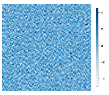
Figure 1: Simulated realization of the Gegenbauer random field.

This article studies minimum contrast estimators (MCEs) of parameters of the Gegenbauer random fields. The MCE methodology has been widely applied in different statistical frameworks (see, for example, Anh et al. [2004, 2007]; WeiLin et al. [2012]). One of the first works which used a MCE methodology for the parameter estimation of spectral densities of stationary processes was the paper by Taniguchi [1987]. Guyon [1995] introduced a class of MCEs for random fields. Anh et al. [2004] derived consistency and asymptotic normality of a class of MCEs for stationary processes within the class of fractional Riesz-Bessel motion (see Anh et al. [1999]). Results based on the second and third-order cumulant spectra were given by Anh et al. [2007]. They also provided asymptotic properties of second and third-order sample spectral functionals. These properties are of independent interest, since they can be applied to study the limiting properties of nonparametric estimators of processes with short or long-range dependence. WeiLin et al. [2012] applied the minimum contrast parameter estimation to approximate the drift parameter of the Ornstein-Uhlenbeck process, when the corresponding stochastic differential equation is driven by the fractional Brownian motion with a specific Hurst index.

A burgeoning literature on spatio-temporal estimation has emerged in recent decades (see Beran et al. [2009], Chan and Tsai [2012], Giraitis et al. [2001], Guo et al. [2009], Li and McLeod [1986], Reisen et al. [2006], among others). One of the most popular estimation tools applied was the maximum likelihood estimation method (MLE). Reisen et al. [2006] addressed the problem of parameter estimation of fractionally integrated processes with seasonal components. In order to estimate the fractional parameters, they propose several log-periodogram regression estimators with different bandwidths selected around and/or between the seasonal frequencies. The same methodology was used by Li and McLeod [1986] for fractionally differenced autoregressive-moving average processes in the stationary time series context. Several contributions have also been made for MLE of long memory spatial processes (see, for example, Anh and Lunney [1995]). For two-dimensional spatial data the paper by Basu and Reinsel [1993] introduced a spatial unilateral first-order autoregressive moving average (ARMA) model. To implement MLE they provided a proper treatment to border cell values with a substantial effect in estimation of parameters. Beran et al. [2009] addressed the problem of the least-squares estimation of autoregressive fractionally integrated moving-average (FARIMA) processes with long-memory. Cohen and Francos [2002] investigated asymptotic properties of least-squares estimators in regression models for two-dimensional random fields. Maximization of the Whittle likelihood has been also considered in the recent literature on the MCE (see for example, Chan and Tsai [2012], Boissy et al. [2005], Leonenko and Sakhno [2006]). Leonenko and Sakhno [2006] gave a continuous version of the Whittle contrast functional supplied with a specific weight function for the estimation of continuous-parameter stochastic processes, deriving the consistency and asymptotic normality of such estimators. Guo et al. [2009] demonstrated that the Whittle maximum likelihood estimator is consistent and asymptotically normal for stationary seasonal autoregressive fractionally integrated moving-average (SARFIMA) processes.

Parameter estimation of stationary Gegenbauer random processes was considered by numerous authors, see, for example, Gray et al. [1989], Chung [1996a, b], Woodward et al. [1998], Collet and Fadili [2006], McElroy and Holan [2012]. Gray et al. [1989] used the generating function of the Gegenbauer polynomials to develop long memory Gegenbauer autoregressive moving-average (GARMA) models that generalize the FARIMA process. GARMA models were estimated by applying the MLE methodology. Chung [1996a] also applied this methodology with slight modifications based on the conditional sum of squares method. Chung [1996b] extended these results to the two-parameter context within the GARMA process class. Woodward et al. [1998] introduced a $k$-factor extension of the GARMA model that allowed to associate the long-memory behavior with each one of the $k$ Gegenbauer frequencies involved.

In this article we restrict our consideration to the estimation of long-range dependence parameters. It is motivated in part by cyclic processes, for which pole locations are known. Also in some applications the spectral density singularity location can be estimated in advance. Various methods, including semiparametric, wavelet, and pseudo-maximum likelihood techniques, of the estimation of a singularity location were discussed by, for example, Arteche and Robinson [2000], Giraitis et al. [2001], and Ferrara and Guégan [2001].

This paper introduces and studies the MCE of parameters of spatial Gegenbauer processes. Specifically, analogous of continuous-space results by Anh et al. [2004] are formulated for random fields defined on integer grids. The consistency and asymptotic normality of the MCE are obtained using a spatial discrete version of the Ibragimov contrast function. The article develops a methodology to practically verify general theoretical assumptions for consistency and asymptotic normality of MCEs for specific models. The results provide a rigorous platform to conduct model selection and statistical inference.

The outline of the article is the following. In section 2, we start by introducing the main notations of the paper. Some fundamental definitions and the main results of this article, Theorem 1 and 2, are given in §3. Section 4 consists of the proofs of the main results. Section 5 presents simulation studies which support the theoretical findings. The Appendix provides auxiliary materials that specify for our case the conditions that ensure the consistency and asymptotic normality of the MCE based on the Ibragimov contrast function formulated in Anh et al. [2004].

In what follows we use the symbol $C$ to denote constants which are not important for our discussion. Moreover, the same symbol $C$ may be used for different constants appearing in the same proof.

All calculations in the article were performed using the software R version 3.0.2 and Maple 16, Maplesoft.

2 Gegenbauer random fields

This section introduces some of the main definitions of the Gegenbauer random fields given in Espejo et al. [2014] (see also, Chung [1996a, b], Gray et al. [1989], and Woodward et al. [1998], for the temporal case).

Let $Y_{t_{1},t_{2}},$ $(t_{1},t_{2})\in\mathbb{Z}^{2},$ be a random field defined on the grid lattice $\mathbb{Z}^{2}.$ Consider the fractional difference operator $\nabla^{d}_{u}$ defined by

$$\nabla^{d}_{u}=(I-2uB+B^{2})^{d}=(1-2\cos\nu B+B^{2})^{d}=[(1-e^{i\nu}B)(1-e^{-i\nu}B)]^{d},$$ (1)

where $B$ is the backward-shift operator, $u=\cos\nu,$ i.e. $\nu=\arccos(u),$ $|u|\leq 1,$ and $d\in\left(-\frac{1}{2},\frac{1}{2}\right).$ Assume that $Y$ satisfies the following state equation

$$\nabla^{d_{1}}_{u_{1}}\circ\nabla^{d_{2}}_{u_{2}}Y_{t_{1},t_{2}}=\left(I-2u_{1}B_{1}+B_{1}^{2}\right)^{d_{1}}\circ\left(I-2u_{2}B_{2}+B_{2}^{2}\right)^{d_{2}}Y_{t_{1},t_{2}}=\varepsilon_{t_{1},t_{2}},$$ (2)

where $\nabla^{d_{i}}_{u_{i}},$ $i=1,2,$ is given by equation (1), with $B_{i},$ $i=1,2,$ denoting the backward-shift operator for each spatial coordinate, i.e. $B_{1}Y_{t_{1},t_{2}}=Y_{t_{1}-1,t_{2}}$, and $B_{2}Y_{t_{1},t_{2}}=Y_{t_{1},t_{2}-1}.$ Here, $\varepsilon_{t_{1},t_{2}},$ $(t_{1},t_{2})\in\mathbb{Z}^{2},$ is a zero-mean white noise field with the common variance $E[\varepsilon_{t_{1},t_{2}}^{2}]=\sigma^{2}_{\varepsilon}.$ The random field $Y$ is called a spatial Gegenbauer white noise in Espejo et al. [2014].

By equation (2) the Gegenbauer random field $Y$ can be defined in terms of the inverse of the operator $\nabla^{d_{1}}_{u_{1}}\circ\nabla^{d_{2}}_{u_{2}}$ expanded in a Gegenbauer polynomial series as follows

$$Y_{t_{1},t_{2}} =\nabla^{-d_{2}}_{u_{2}}\circ\nabla^{-d_{1}}_{u_{1}}\varepsilon_{t_{1},t_{2}}=\sum_{n_{1}=0}^{\infty}\sum_{n_{2}=0}^{\infty}\,C_{n_{1}}^{(d_{1})}(u_{1})\,C_{n_{2}}^{(d_{2})}(u_{2})B_{1}^{n_{1}}B_{2}^{n_{2}}\varepsilon_{t_{1},t_{2}}$$

$$=\sum_{n_{1}=0}^{\infty}\sum_{n_{2}=0}^{\infty}\,C_{n_{1}}^{(d_{1})}(u_{1})\,C_{n_{2}}^{(d_{2})}(u_{2})\varepsilon_{t_{1}-n_{1},t_{2}-n_{2}},$$ (3)

where $d_{i}\neq 0,$ $i=1,2,$ and $C_{n}^{(d)}(u)$ is the Gegenbauer polynomial given by

$$C_{n}^{(d)}(u)=\sum_{k=0}^{[{n}/{2}]}(-1)^{k}\frac{(2u)^{n-2k}\Gamma(d-k+n)}{k!(n-2k)!\Gamma(d)}.$$

The generating function for the Gegenbauer polynomials is given by

$$\sum_{n=0}^{\infty}C_{n}^{(d)}(u)b^{n}=\left(1-2ub+b^{2}\right)^{-d},\quad|b|<1,$$

which explains the expansion of the inverse operator in (3).

In general, a random field $Y$ is called invertible if the white noise $\varepsilon_{t_{1},t_{2}},$ $(t_{1},t_{2})\in\mathbb{Z}^{2},$ can be expressed as the convergent sum

$$\varepsilon_{t_{1},t_{2}}=\sum_{n_{1}=0}^{\infty}\sum_{n_{2}=0}^{\infty}b_{n_{1},n_{2}}Y_{t_{1}-n_{1},t_{2}-n_{2}},$$

where $\sum_{n_{1}=0}^{\infty}\sum_{n_{2}=0}^{\infty}|b_{n_{1},n_{2}}|<\infty.$

The Gegenbauer random field has the following property, see Espejo et al. [2014].

Proposition 1

If $0<d_{i}<\frac{1}{2}$ and $|u_{i}|<1,$ $i=1,2,$ then $Y$ is a stationary invertible long range dependent random field.

The spectral density of a stationary Gegenbauer random field is given by Chung [1996a, b], and Hsu and Tsai [2009], for the one-parameter case, and Espejo et al. [2014], for the two-parameter case:

$$f(\boldsymbol{\lambda},\boldsymbol{\theta}) =\frac{\sigma^{2}_{\varepsilon}}{(2\pi)^{2}}\,\left|1-2u_{1}e^{-i\lambda_{1}}+e^{-2i\lambda_{1}}\right|^{-2d_{1}}\left|1-2u_{2}e^{-i\lambda_{2}}+e^{-2i\lambda_{2}}\right|^{-2d_{2}}$$

$$=\frac{\sigma^{2}_{\varepsilon}}{(2\pi)^{2}}\,\left\{\left|2\cos\lambda_{1}-2u_{1}\right|\right\}^{-2d_{1}}\,\left\{\left|2\cos\lambda_{2}-2u_{2}\right|\right\}^{-2d_{2}},$$ (4)

where $\boldsymbol{\theta}=(\boldsymbol{u},\boldsymbol{d})=(u_{1},u_{2},d_{1},d_{2})\in\Theta=(-1,1)^{2}\times(0,1/2)^{2},$ $u_{i}=\cos\nu_{i}$, and $-\pi\leq\lambda_{i}\leq\pi,$ $i=1,2.$ Using the spectral density function (4), one can compute the auto-covariance function of $Y$ as follows:

$$\gamma(j_{1},j_{2},\boldsymbol{\theta})=\frac{\sigma^{2}_{\varepsilon}}{4\pi}\prod_{i=1}^{2}\Gamma(1-2d_{i})[2\sin(\nu_{i})]^{\frac{1}{2}-2d_{1}}\left[P_{j_{i}-\frac{1}{2}}^{2d_{i}-\frac{1}{2}}(u_{i})+(-1)^{j_{i}}P_{j_{i}-\frac{1}{2}}^{2d_{i}-\frac{1}{2}}(-u_{i})\right],$$

where $P_{a}^{b}(z)$ is the associated Legendre function of the first kind, consult §8 in Abramowitz and Stegun [1972].

From Chung [1996a, b], Gray et al. [1989] and Gradshteyn and Ryzhik [1980], the following asymptotic approximation of the autocovariance function can be obtained

$$\gamma(j_{1},j_{2},\boldsymbol{\theta}) =\prod_{i=1}^{2}\frac{2^{1-2d_{i}}\sigma^{2}_{\epsilon}}{\pi\sin^{2d_{i}}(\nu_{i})}\sin(d_{i}\pi)\Gamma(1-2d_{i})\cos(j_{i}\nu_{i})\frac{\Gamma(j_{i}+2d_{i})}{\Gamma(j_{i}+1)}[1+\mathcal{O}(j_{i}^{-1})].$$

The random field $Y$ is long range dependent as its auto-covariance function satisfies the condition $\sum_{(j_{1},j_{2})\in\mathbb{Z}^{2}}|\gamma(j_{1},j_{2},\boldsymbol{\theta})|=+\infty.$ A detailed discussion on relations between local specifications of spectral functions and the tail behaviour of auto-covariance functions of long range dependent random fields can be found in Leonenko and Olenko [2013].

Figure 2 gives an example of the spectral density and the auto-covariance function of the Gegenbauer random field for the values of the parameters $u_{1}=0.4,$ $u_{2}=0.3,$ $d_{1}=0.2,$ and $d_{2}=0.3.$

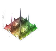
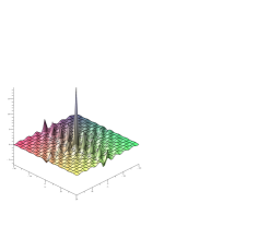
Figure 2: Spectral density and auto-covariance function for $\boldsymbol{u}=(0.4,0.3)$ and $\boldsymbol{d}=(0.2,0.3)$

3 Asymptotic properties of MCEs

Very detailed discussions about estimation of parameters of seasonal/cyclical long memory time series were given in Arteche and Robinson [2000],Giraitis et al. [2001], Ferrara and Guégan [2001], and references therein. It was shown that the case of spectral singularities outside the origin is much more difficult comparing to the situation of a spectral pole at 0. In particular, estimators of parameters $u_{i}$ and $d_{i}$ have different rates of convergence and their joint distributions are still unknown under general conditions.

Ferrara and Guégan [2001] pointed out that, in practice, parameter estimation of seasonal/cyclical long memory data is done in two steps. The first step consists in estimation of singularity locations, which does not represent a difficult issue. Then, the obtained values of location parameters are used in estimators of the long memory parameters. It has been shown that this 2-steps method provides quasi-similar results to simultaneous procedures. Similarly, the results of this paper may also be used in a hierarchical modeling framework. Namely, locations of the singularities can be included in the first level of the hierarchical procedure. Then, on the second step of the hierarchical procedure, the long-range dependence parameters can be estimated by the MCE method, conditioning on the locations obtained on the first step. It also allows to construct a suitable weight function before applying the MCE methodology. Therefore, in this paper we only concentrate our attention on long-range dependence parameters.

Suppose that the conditions imposed in Proposition 1 to ensure stationarity, invertibility and long-range dependence hold. Assume the value of the parameter $\boldsymbol{u}=(u_{1},u_{2})$ is known a priori or was estimated on step 1. Then $\boldsymbol{\theta}=(\theta_{1},\theta_{2})=(d_{1},d_{2})\in\Theta=(0,1/2)^{2}$ is the vector of parameters to estimate of the Gegenbauer random field defined by equation (2) (see also equation (4) for the corresponding spectral density).

Let $Y_{t_{1},t_{2}},$ $t_{1},t_{2}=0,...,T,$ be a part of a realization of the Gegenbauer random field.

Let $w(\boldsymbol{\lambda})$, $\boldsymbol{\lambda}\in[-\pi,\pi]^{2}$, be a nonnegative function. Suppose the condition A3 in the Appendix holds. We define

$$\sigma^{2}(\boldsymbol{\theta})=\displaystyle\int_{[-\pi,\pi]^{2}}f(\boldsymbol{\lambda},\boldsymbol{\theta})w(\boldsymbol{\lambda})\,\,d\boldsymbol{\lambda}$$ (5)

and consider the factorization

$$f(\boldsymbol{\lambda},\boldsymbol{\theta})=\sigma^{2}(\boldsymbol{\theta})\Psi(\boldsymbol{\lambda},\boldsymbol{\theta}).$$ (6)

For all $\boldsymbol{\theta}\in\Theta$ the function $\Psi(\boldsymbol{\lambda},\boldsymbol{\theta})$ has the following property

$$\int_{[-\pi,\pi]^{2}}\Psi(\boldsymbol{\lambda},\boldsymbol{\theta})w(\boldsymbol{\lambda})\,\,d\boldsymbol{\lambda}=1.$$ (7)

Let $K(\boldsymbol{\theta}_{0},\boldsymbol{\theta})$ be a non-random real-valued function, usually referred as the contrast function, given by

$$K(\boldsymbol{\theta_{0}},\boldsymbol{\theta}):=\displaystyle\int_{[-\pi,\pi]^{2}}f(\boldsymbol{\lambda},\boldsymbol{\theta_{0}})w(\boldsymbol{\lambda})\log\frac{\Psi(\boldsymbol{\lambda},\boldsymbol{\theta_{0}})}{\Psi(\boldsymbol{\lambda},\boldsymbol{\theta})}\,\,d\boldsymbol{\lambda},$$

and let the contrast field be

$$U(\boldsymbol{\theta}):=-\displaystyle\int_{[-\pi,\pi]^{2}}f(\boldsymbol{\lambda},\boldsymbol{\theta_{0}})w(\boldsymbol{\lambda})\log\Psi(\boldsymbol{\lambda},\boldsymbol{\theta})\,\,d\boldsymbol{\lambda},$$

where $\boldsymbol{\theta_{0}}=(d_{10},d_{20})$ is the true parameter value. In what follows, $P_{0}$ denotes the probability distribution with the density function $f(\boldsymbol{\lambda},\boldsymbol{\theta}_{0}).$

The empirical version $\hat{U}_{T}(\boldsymbol{\theta}),$ $T\in\mathbb{Z},$ $\boldsymbol{\theta}\in\Theta,$ is defined by

$$\hat{U}_{T}(\boldsymbol{\theta}):=-\displaystyle\int_{[-\pi,\pi]^{2}}I_{T}(\boldsymbol{\lambda})w(\boldsymbol{\lambda})\log\Psi(\boldsymbol{\lambda},\boldsymbol{\theta})\,\,d\boldsymbol{\lambda},$$ (8)

where $I_{T}(\boldsymbol{\lambda})$ is the periodogram of the observations $Y_{t_{1},t_{2}},$ $t_{1},t_{2}=0,...,T,$ of the Gegenbauer random field, that is,

$$I_{T}(\boldsymbol{\lambda}):=\frac{1}{(2\pi T)^{2}}\left|\displaystyle\sum_{t_{1}=0}^{T}\sum_{t_{2}=0}^{T}e^{-i(t_{1}\lambda_{1}+t_{2}\lambda_{2})}Y_{t_{1},t_{2}}\right|^{2}.$$

The MCE is defined by the empirical contrast field $\hat{U}_{T}(\boldsymbol{\theta})$ and the contrast function $K(\boldsymbol{\theta}_{0},\boldsymbol{\theta})$ being $K(\boldsymbol{\theta}_{0},\boldsymbol{\theta})\geq 0,$ and having a unique minimum at $\boldsymbol{\theta}=\boldsymbol{\theta}_{0}.$

In particular, we choose

$$w(\boldsymbol{\lambda})=|\lambda_{1}^{2}-\nu_{1}^{2}|^{a_{1}}|\lambda_{2}^{2}-\nu_{2}^{2}|^{a_{2}}w_{0}(\boldsymbol{\lambda}),\quad\boldsymbol{\lambda}=(\lambda_{1},\lambda_{2})\in[-\pi,\pi]^{2},$$ (9)

where $a_{i}>1,$ $i=1,2,$ $w_{0}(\boldsymbol{\lambda})$ is a positive function with continuous second order derivatives on $[-\pi,\pi]^{2}.$

Notice that by (9) the weight function $w(\boldsymbol{\lambda})$ is nonnegative and symmetric about $(0,0).$ Due to the boundedness of $w(\boldsymbol{\lambda})$ the product $w(\boldsymbol{\lambda})f(\boldsymbol{\lambda},\boldsymbol{\theta})$ is integrable. Thus, the choice of $w(\boldsymbol{\lambda})$ fulfils condition A3 in the Appendix. The developed methodology is readily adjustable to other classes of weight functions.

Theorems 3.1 and 3.2 give consistency and asymptotic normality results for the MCE.

Theorem 3.1

Let $Y_{t_{1},t_{2}},\ (t_{1},t_{2})\in\mathbb{Z}^{2},$ be a stationary Gegenbauer random field which spectral density satisfies equation (4). If $\hat{U}_{T}(\boldsymbol{\theta})$ is the empirical contrast field defined by equation (8), then

• $Y_{t_{1},t_{2}}$ satisfies the conditions A1-A6 in the Appendix;

• the minimum contrast estimator $\hat{\boldsymbol{\theta}}_{T}=(\hat{d}_{1},\hat{d}_{2})=arg\min_{\boldsymbol{\theta}\in\Theta}\,\hat{U}_{T}(\boldsymbol{\boldsymbol{\theta}})\in\Theta$ is a consistent estimator of the parameter vector $\boldsymbol{\theta}.$ That is, there is a convergence in $P_{0}$ probability:

  $$\hat{\boldsymbol{\theta}}_{T}\overset{P_{0}}{\longrightarrow}\boldsymbol{\theta_{0}},\quad T\longrightarrow\infty;$$

• $\hat{\sigma}^{2}_{T}\overset{P_{0}}{\longrightarrow}\sigma^{2}(\boldsymbol{\theta_{0}}),\ T\longrightarrow\infty,$ where the variance estimator $\hat{\sigma}^{2}_{T}$ is given by

  $$\hat{\sigma}^{2}_{T}=\int_{[-\pi,\pi]^{2}}I_{T}(\boldsymbol{\lambda})w(\boldsymbol{\lambda})\,\,d\boldsymbol{\lambda}.$$

Notice that Assumption A4 is not required to prove the last two statements in Theorem 3.1, but it will be used in the proof of Theorem 3.2.

To formulate Theorem 3.2 we introduce the following notations. The unbiased estimator of the correlation function $\gamma(t_{1},t_{2},\boldsymbol{\theta}),$ $\boldsymbol{t}=(t_{1},t_{2})\in\mathbb{Z}^{2},$ of the Gegenbauer random field $Y_{t_{1},t_{2}}$ is

$$\hat{\gamma}_{T}(\boldsymbol{t})=\frac{1}{(T-|t_{1}|)(T-|t_{2}|)}\sum_{k=0}^{T-|t_{1}|}\sum_{l=0}^{T-|t_{2}|}Y_{k,l}Y_{|t_{1}|+k,|t_{2}|+l}.$$

Note that all indices of the random field in the sum above are within the set $\{(t_{1},t_{2}):\,t_{1},t_{2}=0,...,T\},$ where the observations are available.

The unbiased periodogram is given by

$$I_{T}^{*}(\lambda_{1},\lambda_{2})=\frac{1}{(2\pi)^{2}}\sum_{t_{1}=1-T}^{T-1}\sum_{t_{2}=1-T}^{T-1}e^{-i(\lambda_{1}t_{1}+\lambda_{2}t_{2})}\hat{\gamma}_{T}(\boldsymbol{t}),$$

and the corresponding empirical contrast field is

$$\hat{U}_{T}^{*}(\boldsymbol{\theta})=-\displaystyle\int_{[-\pi,\pi]^{2}}I_{T}^{*}(\boldsymbol{\lambda})w(\boldsymbol{\lambda})\log\Psi(\boldsymbol{\lambda},\boldsymbol{\theta})\,\,d\boldsymbol{\lambda}.$$

We also define $\hat{\sigma}^{2*}_{T}=\int_{[-\pi,\pi]^{2}}I_{T}^{*}(\boldsymbol{\lambda})w(\boldsymbol{\lambda})\,\,d\boldsymbol{\lambda}$ and the associated adjusted MCE

$$\hat{\boldsymbol{\theta}}^{*}_{T}=(\hat{d}^{*}_{1},\hat{d}^{*}_{2})=\mbox{arg}\min_{\boldsymbol{\theta}\in\Theta}\,\hat{U}_{T}^{*}(\boldsymbol{\theta}).$$ (10)

Theorem 3.2

If $Y_{t_{1},t_{2}},\ (t_{1},t_{2})\in\mathbb{Z}^{2},$ is a stationary Gegenbauer random field which spectral density satisfies equation (4) with $(d_{1},d_{2})\in(0,1/4)^{2},$ then

• $Y_{t_{1},t_{2}}$ satisfies the conditions A1-A9 in the Appendix;

• the adjusted MCE defined by (10) is asymptotically normal. That is,

  $$T(\hat{\boldsymbol{\theta}}^{*}_{T}-\boldsymbol{\theta}_{0})\stackrel{{\scriptstyle D}}{{\longrightarrow}}\mathcal{N}_{2}(0,\mathbf{S}^{-1}(\boldsymbol{\theta}_{0})A(\boldsymbol{\theta}_{0})\mathbf{S}^{-1}(\boldsymbol{\theta}_{0})),\quad T\longrightarrow\infty,$$

  where the entries of the matrices $\mathbf{S}(\boldsymbol{\theta})=(s_{ij}(\boldsymbol{\theta}))$ and $\mathbf{A}(\boldsymbol{\theta})=(a_{ij}(\boldsymbol{\theta}))$ are

  $${}s_{ij}(\boldsymbol{\theta}) = \displaystyle\int_{[-\pi,\pi]^{2}}f(\boldsymbol{\lambda},\boldsymbol{\theta})w(\boldsymbol{\lambda})\frac{\partial^{2}}{\partial\theta_{i}\partial\theta_{j}}\log\Psi(\boldsymbol{\lambda},\boldsymbol{\theta})\,\,d\boldsymbol{\lambda}=\sigma^{2}(\boldsymbol{\theta})\displaystyle\int_{[-\pi,\pi]^{2}}w(\boldsymbol{\lambda})$$ (11)

  $$\times\left[\frac{\partial^{2}}{\partial\theta_{i}\partial\theta_{j}}\Psi(\boldsymbol{\lambda},\boldsymbol{\theta})-\frac{1}{\Psi(\boldsymbol{\lambda},\boldsymbol{\theta})}\frac{\partial}{\partial\theta_{i}}\Psi(\boldsymbol{\lambda},\boldsymbol{\theta})\frac{\partial}{\partial\theta_{j}}\Psi(\boldsymbol{\lambda},\boldsymbol{\theta})\right]\,d\boldsymbol{\lambda},$$

  $$a_{ij}(\boldsymbol{\theta}) = 8\pi^{2}\displaystyle\int_{[-\pi,\pi]^{2}}f^{2}(\boldsymbol{\lambda},\boldsymbol{\theta})w^{2}(\boldsymbol{\lambda})\frac{\partial}{\partial\theta_{i}}\log\left(\Psi(\boldsymbol{\lambda},\boldsymbol{\theta})\right)\frac{\partial}{\partial\theta_{j}}\log\left(\Psi(\boldsymbol{\lambda},\boldsymbol{\theta})\right)\,\,d\boldsymbol{\lambda}$$ (12)

  $$= 8\pi^{2}\sigma^{4}(\boldsymbol{\theta})\displaystyle\int_{[-\pi,\pi]^{2}}w^{2}(\boldsymbol{\lambda})\frac{\partial}{\partial\theta_{i}}\Psi(\boldsymbol{\lambda},\boldsymbol{\theta})\frac{\partial}{\partial\theta_{j}}\Psi(\boldsymbol{\lambda},\boldsymbol{\theta})\,\,d\boldsymbol{\lambda}.$$

To avoid the edge effect Anh et al. [2004] employed the modified periodogram approach suggested by Guyon [1982]. We use their assumptions in Theorem 3.2. Note that some authors pointed few problems in using $I_{T}^{*},$ see Vidal-Sanz [2009], Yao and Brockwell [2006], and references therein. Various other modifications, for example, typed variograms, smoothed variograms, kernel estimators, to reduce the edge effect have been proposed. It would be interesting to prove analogous of the results by Anh et al. [2004] and Theorem 3.2 for these modifications, too. However, it is beyond the scope of this paper. Moreover, it remains as an open problem whether the edge-effect modification is essential for the asymptotic normality or not, see Yao and Brockwell [2006].

4 Proofs

To prove the theorems we will use the following differentiability lemma.

Lemma 1

[Schilling [2005, Theorem 11.5]] Let $(X,\cal{F},\mu)$ be a measurable space, $A\in\cal{F},$ and $\Theta\subset\mathbb{R}$ be an open set. Suppose the function $F:X\times\Theta\to\mathbb{R}$ satisfies the following conditions:

1. For all $\theta\in\Theta:$ $F(\cdot,\theta)\in L_{1}(A);$

2. For almost all $x\in A$ the derivative $\frac{\partial F(x,\cdot)}{\partial\theta}$ exists for all $\theta\in\Theta;$

3. There is an integrable function $g:X\to\mathbb{R}$ such that $\left|\frac{\partial F(x,\theta)}{\partial\theta}\right|\leq g(x)$ for almost all $x\in A.$

Then there exists $\frac{\partial}{\partial\theta}\int_{A}F(x,\theta)d\mu(x)=\int_{A}\frac{\partial F(x,\theta)}{\partial\theta}d\mu(x).$

Lemma 2

The function $\sigma^{2}(\boldsymbol{\theta})$ is bounded and separated from zero on $\Theta.$ Moreover, its first and second order derivatives are bounded on $\Theta$ and can be computed by

$$\frac{\partial}{\partial\theta_{i}}\sigma^{2}(\boldsymbol{\theta}) = \int_{[-\pi,\pi]^{2}}w(\boldsymbol{\lambda})\frac{\partial}{\partial\theta_{i}}f(\boldsymbol{\lambda},\boldsymbol{\theta})\,d\boldsymbol{\lambda}$$ (13)

$$= -2\int_{[-\pi,\pi]^{2}}\log\left|2\cos\lambda_{i}-2u_{i}\right|\,w(\boldsymbol{\lambda})f(\boldsymbol{\lambda},\boldsymbol{\theta})\,d\boldsymbol{\lambda},$$

$$\frac{\partial^{2}}{\partial\theta_{j}\partial\theta_{i}}\sigma^{2}(\boldsymbol{\theta}) = \displaystyle\int_{[-\pi,\pi]^{2}}w(\boldsymbol{\lambda})\frac{\partial^{2}}{\partial\theta_{j}\partial\theta_{i}}f(\boldsymbol{\lambda},\boldsymbol{\theta})\,d\boldsymbol{\lambda}=4\int_{[-\pi,\pi]^{2}}\log\left|2\cos\lambda_{i}-2u_{i}\right|$$ (14)

$$\times\log\left|2\cos\lambda_{j}-2u_{j}\right|\,w(\boldsymbol{\lambda})f(\boldsymbol{\lambda},\boldsymbol{\theta})\,d\boldsymbol{\lambda},$$

where $i,j=1,2.$

Proof.

By the choice (9) of the weight function we obtain

$$\sup_{[-\pi,\pi]^{2}\times\Theta}f(\boldsymbol{\lambda},\boldsymbol{\theta})w(\boldsymbol{\lambda})<+\infty$$ (15)

and

$$\sup_{\theta\in\Theta}\sigma^{2}(\boldsymbol{\theta})=\int_{[-\pi,\pi]^{2}}\sup_{\theta\in\Theta}f(\boldsymbol{\lambda},\boldsymbol{\theta})w(\boldsymbol{\lambda})d\boldsymbol{\lambda}\leq 4\pi^{2}\sup_{[-\pi,\pi]^{2}\times\Theta}f(\boldsymbol{\lambda},\boldsymbol{\theta})w(\boldsymbol{\lambda})<+\infty.$$

Hence, $\sigma^{2}(\boldsymbol{\theta})$ is bounded.

Note that $\sup_{[-\pi,\pi]^{2}\times\Theta}\left\{\left|2\cos\lambda_{1}-2u_{1}\right|\right\}^{2d_{1}}\,\left\{\left|2\cos\lambda_{2}-2u_{2}\right|\right\}^{2d_{2}}<+\infty.$ Also, by the choice of the weight function, there exists $\delta>0$ and a set $A_{0}\subset[-\pi,\pi]^{2}$ of non-zero Lebesgue measure such that $w(\boldsymbol{\lambda})>\delta$ for all $\boldsymbol{\lambda}\in A_{0}.$ Therefore,

$$\inf_{\theta\in\Theta}\sigma^{2}(\boldsymbol{\theta}) =\inf_{\theta\in\Theta}\int_{[-\pi,\pi]^{2}}f(\boldsymbol{\lambda},\boldsymbol{\theta})w(\boldsymbol{\lambda})d\boldsymbol{\lambda}$$

$$\geq\frac{\delta\,\boldsymbol{\lambda}(A_{0})}{\sup_{[-\pi,\pi]^{2}\times\Theta}\left\{\left|2\cos\lambda_{1}-2u_{1}\right|\right\}^{2d_{1}}\,\left\{\left|2\cos\lambda_{2}-2u_{2}\right|\right\}^{2d_{2}}}>0,$$

which means that $\sigma^{2}(\boldsymbol{\theta})$ is separated from zero on $\Theta.$

Now, to study $\frac{\partial}{\partial\theta_{i}}\sigma^{2}(\boldsymbol{\theta})$ we compute $\frac{\partial}{\partial\theta_{i}}f(\boldsymbol{\lambda},\boldsymbol{\theta}),$ $i=1,2:$

$$\frac{\partial}{\partial\theta_{i}}f(\boldsymbol{\lambda},\boldsymbol{\theta}) =\frac{\sigma^{2}_{\varepsilon}}{(2\pi)^{2}}\left\{\left|2\cos\lambda_{j}-2u_{j}\right|\right\}^{-2d_{j}}\frac{\partial}{\partial d_{i}}\left\{\left|2\cos\lambda_{i}-2u_{i}\right|\right\}^{-2d_{i}}$$

$$=\log\left(\left(2\cos\lambda_{i}-2u_{i}\right)^{-2}\right)\frac{\sigma^{2}_{\varepsilon}}{(2\pi)^{2}}\left[2(\cos\lambda_{i}-u_{i})\right]^{-2d_{i}}$$

$$\quad\times\left[2(\cos\lambda_{j}-u_{j})\right]^{-2d_{j}}=-2\log\left|2\cos\lambda_{i}-2u_{i}\right|f(\boldsymbol{\lambda},\boldsymbol{\theta}),$$ (16)

where $j\not=i$ and $j=1,2.$

Using (9) and (16) we conclude that

$$\sup_{[-\pi,\pi]^{2}\times\Theta}\left|w(\boldsymbol{\lambda})\frac{\partial}{\partial\theta_{i}}f(\boldsymbol{\lambda},\boldsymbol{\theta})\right|<+\infty.$$ (17)

Thus, by (5) and Lemma 1 there exists

$$\frac{\partial}{\partial\theta_{i}}\sigma^{2}(\boldsymbol{\theta})=\displaystyle\int_{[-\pi,\pi]^{2}}w(\boldsymbol{\lambda})\frac{\partial}{\partial\theta_{i}}f(\boldsymbol{\lambda},\boldsymbol{\theta})\,\,d\boldsymbol{\lambda}$$

and

$$\sup_{\Theta}\left|\frac{\partial}{\partial\theta_{i}}\sigma^{2}(\boldsymbol{\theta})\right|\leq 4\pi^{2}\sup_{[-\pi,\pi]^{2}\times\Theta}\left|w(\boldsymbol{\lambda})\frac{\partial}{\partial\theta_{i}}f(\boldsymbol{\lambda},\boldsymbol{\theta})\right|<+\infty.$$

It is not difficult to find $\frac{\partial^{2}}{\partial\theta_{i}\partial\theta_{j}}f(\boldsymbol{\lambda},\boldsymbol{\theta}).$ By (16), for $i,j=1,2,$ $i\neq j,$ the second derivatives of $f$ are given by

$$\frac{\partial^{2}}{\partial\theta^{2}_{i}}f(\boldsymbol{\lambda},\boldsymbol{\theta})=-2\log\left|2\cos\lambda_{i}-2u_{i}\right|\frac{\partial}{\partial\theta_{i}}f(\boldsymbol{\lambda},\boldsymbol{\theta})=4\left(\log\left|2\cos\lambda_{i}-2u_{i}\right|\right)^{2}f(\boldsymbol{\lambda},\boldsymbol{\theta}),$$ (18)

$$\frac{\partial^{2}}{\partial\theta_{j}\partial\theta_{i}}f(\boldsymbol{\lambda},\boldsymbol{\theta})=4\log\left|2\cos\lambda_{i}-2u_{i}\right|\cdot\log\left|2\cos\lambda_{j}-2u_{j}\right|f(\boldsymbol{\lambda},\boldsymbol{\theta}).$$ (19)

It follows from (18), (19), and (9) that

$$\sup_{[-\pi,\pi]^{2}\times\Theta}\left|w(\boldsymbol{\lambda})\frac{\partial^{2}}{\partial\theta_{j}\partial\theta_{i}}f(\boldsymbol{\lambda},\boldsymbol{\theta})\right|<+\infty,\quad i,j=1,2.$$ (20)

Finally, by (13) and Lemma 1 there exists

$$\frac{\partial^{2}}{\partial\theta_{j}\partial\theta_{i}}\sigma^{2}(\boldsymbol{\theta})=\displaystyle\int_{[-\pi,\pi]^{2}}w(\boldsymbol{\lambda})\frac{\partial^{2}}{\partial\theta_{j}\partial\theta_{i}}f(\boldsymbol{\lambda},\boldsymbol{\theta})\,\,d\boldsymbol{\lambda}$$

and

$$\sup_{\Theta}\left|\frac{\partial^{2}}{\partial\theta_{j}\partial\theta_{i}}\sigma^{2}(\boldsymbol{\theta})\right|\leq 4\pi^{2}\sup_{[-\pi,\pi]^{2}\times\Theta}\left|w(\boldsymbol{\lambda})\frac{\partial^{2}}{\partial\theta_{j}\partial\theta_{i}}f(\boldsymbol{\lambda},\boldsymbol{\theta})\right|<+\infty.\vspace{-3mm}$$ (21)

$\vspace{-3mm}\blacksquare$ ∎

Proof.

of Theorem 3.1. We will prove that the conditions A1-A6 in the Appendix are satisfied. Therefore, we will be able to apply Theorem 3 by Anh et al. [2004] and obtain the statement of Theorem 3.1.

The condition A1 holds, since $\boldsymbol{\theta}_{0}$ belongs to the parameter space $\Theta=\left(0,\frac{1}{2}\right)^{2}$ which is an interior of the compact set $\left[0,\frac{1}{2}\right]^{2}$.

It follows from representation (4) of the spectral density that $f(\boldsymbol{\lambda},\boldsymbol{\theta}_{1})\neq f(\boldsymbol{\lambda},\boldsymbol{\theta}_{2}),$ for $\boldsymbol{\theta}_{1}\neq\boldsymbol{\theta}_{2}.$ Thus, the condition A2 is satisfied.

The class of non-negative weight functions $w(\boldsymbol{\lambda})$ defined by (9) consists of symmetric functions. Note that

$$|\cos(\lambda_{i})-\cos(\nu_{i})|=2\left|\sin\left(\frac{\lambda_{i}+\nu_{i}}{2}\right)\sin\left(\frac{\lambda_{i}-\nu_{i}}{2}\right)\right|\sim C\,|\lambda_{i}^{2}-\nu_{i}^{2}|,$$

when $\lambda_{i}\to\pm\nu_{i}.$ Thus, by (9) and representation (4) of the spectral density we get $w(\boldsymbol{\lambda})f(\boldsymbol{\lambda},\boldsymbol{\theta})\in L_{1}([-\pi,\pi]^{2})$ for all $\boldsymbol{\theta}.$

To verify A4, that is, to prove

$$\nabla_{\boldsymbol{\theta}}\displaystyle\int_{[-\pi,\pi]^{2}}\Psi(\boldsymbol{\lambda},\boldsymbol{\theta})w(\boldsymbol{\lambda})\,\,d\boldsymbol{\lambda}=\displaystyle\int_{[-\pi,\pi]^{2}}\nabla_{\boldsymbol{\theta}}\Psi(\boldsymbol{\lambda},\boldsymbol{\theta})w(\boldsymbol{\lambda})\,\,d\boldsymbol{\lambda}=0,$$

we find

$$w(\boldsymbol{\lambda})\frac{\partial}{\partial\theta_{i}}\Psi(\boldsymbol{\lambda},\boldsymbol{\theta})=\underbrace{\frac{w(\boldsymbol{\lambda})}{\sigma^{2}(\boldsymbol{\theta})}\left[\frac{\partial}{\partial\theta_{i}}f(\boldsymbol{\lambda},\boldsymbol{\theta})\right]}_{S_{1}(\boldsymbol{\lambda},\boldsymbol{\theta})}-\underbrace{\frac{w(\boldsymbol{\lambda})}{\sigma^{4}(\boldsymbol{\theta})}\left[\frac{\partial}{\partial\theta_{i}}\sigma^{2}(\boldsymbol{\theta})\right]f(\boldsymbol{\lambda},\boldsymbol{\theta})}_{S_{2}(\boldsymbol{\lambda},\boldsymbol{\theta})}$$ (22)

and apply Lemma 1.

The same symbol $C$ is used for different nonessential constants appearing in the calculations below.

By (4) and the choice of the weight function we obtain

$$\sup_{[-\pi,\pi]^{2}\times\Theta}\big{|}\log\left|2\cos\lambda_{i}-2u_{i}\right|\big{|}\,f(\boldsymbol{\lambda},\boldsymbol{\theta})w(\boldsymbol{\lambda})<+\infty.$$ (23)

Therefore, by equation (16) and Lemma 2:

$$|S_{1}(\boldsymbol{\lambda},\boldsymbol{\theta})|\leq\frac{C}{\sigma^{2}(\boldsymbol{\theta})}\leq\frac{C}{\min_{\Theta}\sigma^{2}(\boldsymbol{\theta})}\in L_{1}([-\pi,\pi]^{2}).$$ (24)

Now, by (15), (22) and Lemma 2 we can estimate $S_{2}(\boldsymbol{\lambda},\boldsymbol{\theta})$ as

$$\left|S_{2}(\boldsymbol{\lambda},\boldsymbol{\theta})\right|=\left|w(\boldsymbol{\lambda})\frac{\left[\frac{\partial}{\partial\theta_{i}}\sigma^{2}(\boldsymbol{\theta})\right]f(\boldsymbol{\lambda},\boldsymbol{\theta})}{\sigma^{4}(\boldsymbol{\theta})}\right|\leq C\,\frac{w(\boldsymbol{\lambda})f(\boldsymbol{\lambda},\boldsymbol{\theta})}{\min_{\Theta}\sigma^{4}(\boldsymbol{\theta})}\leq C.$$ (25)

Finally, A4 follows from (24), (25), and Lemma 1 with $g(x)=C.$

Note that $L_{1}([-\pi,\pi]^{2})\cap L_{2}([-\pi,\pi]^{2})=L_{2}([-\pi,\pi]^{2}).$ To verify the condition A5 for the weight function $w(\cdot)$ we have to show that $f(\boldsymbol{\lambda},\boldsymbol{\theta}_{0})w(\boldsymbol{\lambda})\cdot$ $\log\Psi(\boldsymbol{\lambda},\boldsymbol{\theta})\in L_{2}([-\pi,\pi]^{2}),$ for all $\boldsymbol{\theta}\in\Theta.$ By (4) and (9) the product $f(\boldsymbol{\lambda},\boldsymbol{\theta}_{0})\cdot$ $w(\boldsymbol{\lambda})\log\Psi(\boldsymbol{\lambda},\boldsymbol{\theta})$ is bounded for all $\boldsymbol{\lambda}$ except $\{\boldsymbol{\lambda}:\lambda_{i}=\pm\nu_{i},\ i=1,2\}.$ Let $\tilde{d}_{i}=\max({d}_{i},{d}_{i0}).$ Then, for $\lambda_{i}\to\pm\nu_{i},$ $i=1,2:$

$$[f(\boldsymbol{\lambda},\boldsymbol{\theta}_{0})w(\boldsymbol{\lambda})\log\Psi(\boldsymbol{\lambda},\boldsymbol{\theta})]^{2}\leq C\prod_{i=1}^{2}|{\lambda_{i}}\pm{\nu_{i}}|^{2a_{i}-4\tilde{d}_{i}}\log|\lambda_{i}\pm\nu_{i}|\in L_{1}([-\pi,\pi]^{2}).$$

Therefore, combining the above results we conclude that A5 holds.

To verify the condition A6 we use the following function $v(\boldsymbol{\lambda})=|\lambda_{1}^{2}-\nu_{1}^{2}|^{\beta}|\lambda_{2}^{2}-\nu_{2}^{2}|^{\beta},$ $\beta\in(0,1/2).$ Note that

$$\frac{|\lambda_{1}^{2}-\nu_{1}^{2}|^{\beta}}{|\lambda_{2}^{2}-\nu_{2}^{2}|^{-\beta}}\log f(\boldsymbol{\lambda},\boldsymbol{\theta})\sim C\frac{|\lambda_{1}^{2}-\nu_{1}^{2}|^{\beta}}{|\lambda_{2}^{2}-\nu_{2}^{2}|^{-\beta}}\left(d_{1}\log|\lambda_{1}^{2}-\nu_{1}^{2}|+d_{2}\log|\lambda_{1}^{2}-\nu_{1}^{2}|\right)\to 0,$$

when $\lambda_{i}\to\pm\nu_{i}.$ Thus, by the choice of $v(\cdot)$ and properties of $\sigma(\boldsymbol{\theta})$ the function

$$h(\boldsymbol{\lambda},\boldsymbol{\theta})=v(\boldsymbol{\lambda})\log\Psi(\boldsymbol{\lambda},\boldsymbol{\theta})=|\lambda_{1}^{2}-\nu_{1}^{2}|^{\beta}|\lambda_{2}^{2}-\nu_{2}^{2}|^{\beta}\left(\log f(\boldsymbol{\lambda},\boldsymbol{\theta})-2\log\sigma(\boldsymbol{\theta})\right)$$

is uniformly continuous on $[-\pi,\pi]^{2}\times\Theta.$

Also, it holds

$$\left|f(\boldsymbol{\lambda},\boldsymbol{\theta}_{0})\frac{w(\boldsymbol{\lambda})}{v(\boldsymbol{\lambda})}\right|\leq Cv^{-1}(\boldsymbol{\lambda})\in L_{2}([-\pi,\pi]^{2}).$$

Since the conditions A1-A6 are satisfied Theorem 1 follows from Theorem 3 in Anh et al. [2004]. $\blacksquare$ ∎

Proof.

of Theorem 2. To prove the asymptotic normality of the MCE in Theorem 3.2 we will show that the conditions A7-A9 of the Appendix hold.

We begin by proving the condition A7. First, to verify the twice differentiability of the function $\Psi(\boldsymbol{\lambda},\boldsymbol{\boldsymbol{\theta}})$ on $\Theta$ we formally compute the second-order derivatives of $\Psi:$

$$\frac{\partial^{2}}{\partial\theta_{j}\partial\theta_{i}}\Psi(\boldsymbol{\lambda},\boldsymbol{\boldsymbol{\theta}}) = \frac{\partial}{\partial\theta_{j}}\left[\frac{\left[\frac{\partial}{\partial\theta_{i}}f(\boldsymbol{\lambda},\boldsymbol{\theta})\right]\sigma^{2}(\boldsymbol{\theta})-\left[\frac{\partial}{\partial\theta_{i}}\sigma^{2}(\boldsymbol{\theta})\right]f(\boldsymbol{\lambda},\boldsymbol{\theta})}{\sigma^{4}(\boldsymbol{\theta})}\right]$$

$$= \frac{1}{\sigma^{4}(\boldsymbol{\theta})}\left\{\left[\frac{\partial^{2}}{\partial\theta_{j}\partial\theta_{i}}f(\boldsymbol{\lambda},\boldsymbol{\theta})\right]\sigma^{2}(\boldsymbol{\theta})+\left[\frac{\partial}{\partial\theta_{j}}\sigma^{2}(\boldsymbol{\theta})\right]\left[\frac{\partial}{\partial\theta}_{i}f(\boldsymbol{\lambda},\boldsymbol{\theta})\right]\right\}$$

$$- \frac{1}{\sigma^{4}(\boldsymbol{\theta})}\left\{\left[\frac{\partial^{2}}{\partial\theta_{j}\partial\theta_{i}}\sigma^{2}(\boldsymbol{\theta})\right]f(\boldsymbol{\lambda},\boldsymbol{\theta})-\left[\frac{\partial}{\partial\theta_{i}}\sigma^{2}(\boldsymbol{\theta})\right]\left[\frac{\partial}{\partial\theta_{j}}f(\boldsymbol{\lambda},\boldsymbol{\theta})\right]\right\}$$

$$- \frac{1}{\sigma^{8}(\boldsymbol{\theta})}\left\{\frac{\partial}{\partial\theta_{j}}\sigma^{4}(\boldsymbol{\theta})\left(\left[\frac{\partial}{\partial\theta_{i}}f(\boldsymbol{\lambda},\boldsymbol{\theta})\right]\sigma^{2}(\boldsymbol{\theta})-\left[\frac{\partial}{\partial\theta_{i}}\sigma^{2}(\boldsymbol{\theta})\right]f(\boldsymbol{\lambda},\boldsymbol{\theta})\right)\right\}.$$

Note that in Lemma 2 we proved that the derivatives $\frac{\partial}{\partial\theta_{i}}\sigma^{2}(\boldsymbol{\theta}),$ $\frac{\partial^{2}}{\partial\theta_{j}\partial\theta_{i}}\sigma^{2}(\boldsymbol{\theta}),$ $\frac{\partial}{\partial\theta_{i}}f(\boldsymbol{\lambda},\boldsymbol{\theta}),$ and $\frac{\partial^{2}}{\partial\theta_{i}\partial\theta_{j}}f(\boldsymbol{\lambda},\boldsymbol{\theta})$ exist. Hence, by the above computations and Lemma 2 the function $\Psi$ is twice differentiable on $\Theta.$

In addition, by estimates (17), (20), (21), Lemma 2, and the above representation for $\frac{\partial^{2}}{\partial\theta_{j}\partial\theta_{i}}\Psi(\boldsymbol{\lambda},\boldsymbol{\boldsymbol{\theta}})$ the product $w(\boldsymbol{\lambda})f(\boldsymbol{\lambda},\boldsymbol{\theta}_{0})\frac{\partial^{2}}{\partial\theta_{i}\partial\theta_{j}}\log\Psi(\boldsymbol{\lambda},\boldsymbol{\theta})$ is bounded on $[-\pi,\pi]^{2}\times\Theta.$ Hence, for $i,j=1,2,$ $\boldsymbol{\theta}\in\Theta:$

$$w(\boldsymbol{\lambda})f(\boldsymbol{\lambda},\boldsymbol{\theta}_{0})\frac{\partial^{2}}{\partial\theta_{i}\partial\theta_{j}}\log\Psi(\boldsymbol{\lambda},\boldsymbol{\theta})\in L_{1}([-\pi,\pi]^{2})\cap L_{2}([-\pi,\pi]^{2}).$$

To prove part 2 of the condition A7, we first note that by (6) and (16):

$$\frac{\partial}{\partial\theta_{i}}\log\Psi(\boldsymbol{\lambda},\boldsymbol{\theta})=-2\log\left|2\cos\lambda_{i}-2u_{i}\right|-\frac{\frac{\partial}{\partial\theta_{i}}\sigma^{2}(\boldsymbol{\theta})}{\sigma^{4}(\boldsymbol{\theta})}.$$

By Lemma 2 the second term is bounded. Hence, it follows from (15) and (23) that the product $w(\boldsymbol{\lambda})f(\boldsymbol{\lambda},\boldsymbol{\theta}_{0})\frac{\partial}{\partial\theta_{i}}\log\Psi(\boldsymbol{\lambda},\boldsymbol{\theta})$ is bounded on $[-\pi,\pi]^{2}\times\Theta,$ that implies

$$w(\boldsymbol{\lambda})f(\boldsymbol{\lambda},\boldsymbol{\theta}_{0})\frac{\partial}{\partial\theta_{i}}\log\Psi(\boldsymbol{\lambda},\boldsymbol{\theta})\in L_{k}([-\pi,\pi]^{2}),\quad k\geq 1,\ \ i=1,2,\ \ \boldsymbol{\theta}\in\Theta.$$

To verify the condition A8 we first check the positive definiteness of the matrices $S(\boldsymbol{\theta})$ and $\mathbf{A}(\boldsymbol{\theta}).$

The entries of $S(\boldsymbol{\theta})$ can be rewritten as

$$s_{i,j}(\boldsymbol{\theta})=\sigma^{2}(\boldsymbol{\theta})\int_{[-\pi,\pi]^{2}}\Psi_{w}(\boldsymbol{\lambda},\boldsymbol{\theta})\frac{\partial^{2}}{\partial\theta_{i}\partial\theta_{j}}\log\Psi_{w}(\boldsymbol{\lambda},\boldsymbol{\theta})d\boldsymbol{\lambda},$$

where $\Psi_{w}(\boldsymbol{\lambda},\boldsymbol{\theta})=f(\boldsymbol{\lambda},\boldsymbol{\theta})w(\boldsymbol{\lambda})/\sigma^{2}(\boldsymbol{\theta}).$

By (4), (9), and Lemma 2 the function $\Psi_{w}(\boldsymbol{\lambda},\boldsymbol{\theta})$ is integrable, i.e. there is a constant $C$ such that $\Psi_{w}(\boldsymbol{\lambda},\boldsymbol{\theta})/C$ is a density. Hence, $S(\boldsymbol{\theta})=C\sigma^{2}(\boldsymbol{\theta}){\cal I}(\theta),$ where $\cal I$ is the Fisher information matrix of the random vector $\tilde{\boldsymbol{X}}$ with the density $\tilde{\Psi}_{w}(\boldsymbol{\lambda},\boldsymbol{\theta})=\Psi_{w}(\boldsymbol{\lambda},\boldsymbol{\theta})/\int_{[-\pi,\pi]^{2}}\Psi_{w}(\boldsymbol{\lambda},\boldsymbol{\theta})d\boldsymbol{\lambda}.$ Therefore, $S(\boldsymbol{\theta})$ is non-negative definite. Note that ${\cal I}(\theta)=-\left(E\left(\tilde{Q}_{i}\tilde{Q}_{j}\right)\right)_{i,j=1,2},$ where $\tilde{Q}_{i}=\frac{\partial}{\partial\theta_{i}}\tilde{\Psi}_{w}(\tilde{\boldsymbol{X}},\boldsymbol{\theta}).$ The random variables $\tilde{Q}_{1}$ and $\tilde{Q}_{2}$ are not a.s. linearly related which implies positive definiteness of $S(\boldsymbol{\theta})$ .

The entries of $A(\boldsymbol{\theta})$ can be rewritten as

$$a_{i,j}(\boldsymbol{\theta})=8\pi^{2}\sigma^{4}(\boldsymbol{\theta})\displaystyle\int_{[-\pi,\pi]^{2}}w^{2}(\boldsymbol{\lambda})\frac{\partial}{\partial\theta_{i}}\Psi(\boldsymbol{\lambda},\boldsymbol{\theta})\frac{\partial}{\partial\theta_{j}}\Psi(\boldsymbol{\lambda},\boldsymbol{\theta})\,d\boldsymbol{\lambda}=C\sigma^{4}(\boldsymbol{\theta})\,E\left(Q_{i}Q_{j}\right),$$

where $Q_{i}=\frac{\partial}{\partial\theta_{i}}\Psi(\boldsymbol{X},\boldsymbol{\theta})$ and the random vector $\boldsymbol{X}$ has the density $\frac{w^{2}(\boldsymbol{\lambda})}{\int_{[-\pi,\pi]^{2}}w^{2}(\boldsymbol{\lambda})\,d\boldsymbol{\lambda}}.$

As $\left(E\left(Q_{i}Q_{j}\right)\right)_{i,j=1,2}$ is a non-negative definite matrix, $A(\boldsymbol{\theta})$ is non-negative definite too. Moreover, it is positive definite, because the random variables $Q_{1}$ and $Q_{2}$ are not a.s. linearly related.

Now we compute elements of the matrix $S(\boldsymbol{\theta}).$ By (11)

$$s_{i,j}(\boldsymbol{\theta}) = \sigma^{2}(\boldsymbol{\theta})\int_{[-\pi,\pi]^{2}}w(\boldsymbol{\lambda})\left[\frac{\partial^{2}}{\partial\theta_{i}\partial\theta_{j}}\Psi(\boldsymbol{\lambda},\boldsymbol{\theta})-\frac{1}{\Psi(\boldsymbol{\lambda},\boldsymbol{\theta})}\frac{\partial}{\partial\theta_{i}}\Psi(\boldsymbol{\lambda},\boldsymbol{\theta})\frac{\partial}{\partial\theta_{j}}\Psi(\boldsymbol{\lambda},\boldsymbol{\theta})\right]d\boldsymbol{\lambda}$$

$$= \sigma^{2}(\boldsymbol{\theta})\int_{[-\pi,\pi]^{2}}\left(w(\boldsymbol{\lambda})\frac{\partial}{\partial\theta_{j}}\left[\frac{\left[\frac{\partial}{\partial\theta_{i}}f(\boldsymbol{\lambda},\boldsymbol{\theta})\right]\sigma^{2}(\boldsymbol{\theta})-\left[\frac{\partial}{\partial\theta_{i}}\sigma^{2}(\boldsymbol{\theta})\right]f(\boldsymbol{\lambda},\boldsymbol{\theta})}{\sigma^{4}(\boldsymbol{\theta})}\right]\right.$$

$$-\frac{w(\boldsymbol{\lambda})}{f(\boldsymbol{\lambda},\boldsymbol{\theta})\sigma^{6}(\boldsymbol{\theta})}\left(\left[\frac{\partial}{\partial\theta_{i}}f(\boldsymbol{\lambda},\boldsymbol{\theta})\right]\sigma^{2}(\boldsymbol{\theta})-\left[\frac{\partial}{\partial\theta_{i}}\sigma^{2}(\boldsymbol{\theta})\right]f(\boldsymbol{\lambda},\boldsymbol{\theta})\right)$$

$$\left.\times\left(\left[\frac{\partial}{\partial\theta_{j}}f(\boldsymbol{\lambda},\boldsymbol{\theta})\right]\sigma^{2}(\boldsymbol{\theta})-\left[\frac{\partial}{\partial\theta_{j}}\sigma^{2}(\boldsymbol{\theta})\right]f(\boldsymbol{\lambda},\boldsymbol{\theta})\right)\right)d\boldsymbol{\lambda}$$

$$= \int_{[-\pi,\pi]^{2}}\left(\frac{w(\boldsymbol{\lambda})}{\sigma^{2}(\boldsymbol{\theta})}\left(\left[\frac{\partial^{2}}{\partial\theta_{j}\partial\theta_{i}}f(\boldsymbol{\lambda},\boldsymbol{\theta})\right]\sigma^{2}(\boldsymbol{\theta})+\left[\frac{\partial}{\partial\theta_{j}}\sigma^{2}(\boldsymbol{\theta})\right]\left[\frac{\partial}{\partial\theta}_{i}f(\boldsymbol{\lambda},\boldsymbol{\theta})\right]\right)\right.$$

$$-\frac{w(\boldsymbol{\lambda})}{\sigma^{2}(\boldsymbol{\theta})}\left(\left[\frac{\partial^{2}}{\partial\theta_{j}\partial\theta_{i}}\sigma^{2}(\boldsymbol{\theta})\right]f(\boldsymbol{\lambda},\boldsymbol{\theta})-\left[\frac{\partial}{\partial\theta_{i}}\sigma^{2}(\boldsymbol{\theta})\right]\left[\frac{\partial}{\partial\theta_{j}}f(\boldsymbol{\lambda},\boldsymbol{\theta})\right]\right)$$

$$-2\frac{w(\boldsymbol{\lambda})}{\sigma^{6}(\boldsymbol{\theta})}\left(\frac{\partial}{\partial\theta_{j}}\sigma^{2}(\boldsymbol{\theta})\left(\left[\frac{\partial}{\partial\theta_{i}}f(\boldsymbol{\lambda},\boldsymbol{\theta})\right]\sigma^{2}(\boldsymbol{\theta})-\left[\frac{\partial}{\partial\theta_{i}}\sigma^{2}(\boldsymbol{\theta})\right]f(\boldsymbol{\lambda},\boldsymbol{\theta})\right)\right)$$

$$-\frac{w(\boldsymbol{\lambda})}{\sigma^{4}(\boldsymbol{\theta})f(\boldsymbol{\lambda},\boldsymbol{\theta})}\left(\left[\frac{\partial}{\partial\theta_{i}}f(\boldsymbol{\lambda},\boldsymbol{\theta})\right]\sigma^{2}(\boldsymbol{\theta})-\left[\frac{\partial}{\partial\theta_{i}}\sigma^{2}(\boldsymbol{\theta})\right]f(\boldsymbol{\lambda},\boldsymbol{\theta})\right)$$

$$\times\left(\left[\frac{\partial}{\partial\theta_{j}}f(\boldsymbol{\lambda},\boldsymbol{\theta})\right]\sigma^{2}(\boldsymbol{\theta})-\left[\frac{\partial}{\partial\theta_{j}}\sigma^{2}(\boldsymbol{\theta})\right]f(\boldsymbol{\lambda},\boldsymbol{\theta})\right)d\boldsymbol{\lambda}.$$

By (5), (13), (14), and (16) we obtain

$$s_{i,j}(\boldsymbol{\theta})=3\int_{[-\pi,\pi]^{2}}\frac{w(\boldsymbol{\lambda})}{\sigma^{2}(\boldsymbol{\theta})}\left[\frac{\partial}{\partial\theta_{j}}\sigma^{2}(\boldsymbol{\theta})\right]\left[\frac{\partial}{\partial\theta}_{i}f(\boldsymbol{\lambda},\boldsymbol{\theta})\right]d\boldsymbol{\lambda}$$

$$-\int_{[-\pi,\pi]^{2}}\frac{w(\boldsymbol{\lambda})}{f(\boldsymbol{\lambda},\boldsymbol{\theta})}\left[\frac{\partial}{\partial\theta_{i}}f(\boldsymbol{\lambda},\boldsymbol{\theta})\right]\left[\frac{\partial}{\partial\theta_{j}}f(\boldsymbol{\lambda},\boldsymbol{\theta})\right]d\boldsymbol{\lambda}=\frac{3}{\sigma^{2}(\boldsymbol{\theta})}\left[\frac{\partial}{\partial\theta_{j}}\sigma^{2}(\boldsymbol{\theta})\right]\left[\frac{\partial}{\partial\theta_{i}}\sigma^{2}(\boldsymbol{\theta})\right]$$

$$-4\int_{[-\pi,\pi]^{2}}\log\left|2\cos\lambda_{i}-2u_{i}\right|\log\left|2\cos\lambda_{j}-2u_{j}\right|\,w(\boldsymbol{\lambda})f(\boldsymbol{\lambda},\boldsymbol{\theta})d\boldsymbol{\lambda}.$$

By (12) the elements of the matrix $A(\boldsymbol{\theta})$ are

$$a_{i,j}(\boldsymbol{\theta}) = 8\pi^{2}\sigma^{4}(\boldsymbol{\theta})\int_{[-\pi,\pi]^{2}}w^{2}(\boldsymbol{\lambda})\frac{\partial}{\partial\theta_{i}}\Psi(\boldsymbol{\lambda},\boldsymbol{\theta})\frac{\partial}{\partial\theta_{j}}\Psi(\boldsymbol{\lambda},\boldsymbol{\theta})\,d\boldsymbol{\lambda}$$

$$= 8\pi^{2}\int_{[-\pi,\pi]^{2}}w^{2}(\boldsymbol{\lambda})\left(\left[\frac{\partial}{\partial\theta_{i}}f(\boldsymbol{\lambda},\boldsymbol{\theta})\right]\sigma^{2}(\boldsymbol{\theta})-\left[\frac{\partial}{\partial\theta_{i}}\sigma^{2}(\boldsymbol{\theta})\right]f(\boldsymbol{\lambda},\boldsymbol{\theta})\right)$$

$$\times\left(\left[\frac{\partial}{\partial\theta_{j}}f(\boldsymbol{\lambda},\boldsymbol{\theta})\right]\sigma^{2}(\boldsymbol{\theta})-\left[\frac{\partial}{\partial\theta_{j}}\sigma^{2}(\boldsymbol{\theta})\right]f(\boldsymbol{\lambda},\boldsymbol{\theta})\right)\,d\boldsymbol{\lambda}.$$

Hence, by (16) we get $a_{i,j}(\boldsymbol{\theta})=S_{1}-S_{2}(i,j)-S_{2}(j,i)+S_{3},$ where

$$S_{1}=32\pi^{2}\sigma^{4}(\boldsymbol{\theta})\int_{[-\pi,\pi]^{2}}\log\left|2\cos\lambda_{i}-2u_{i}\right|\log\left|2\cos\lambda_{j}-2u_{j}\right|\,w^{2}(\boldsymbol{\lambda})f^{2}(\boldsymbol{\lambda},\boldsymbol{\theta})d\boldsymbol{\lambda},\vspace{-4mm}$$

$$S_{2}(i,j) = 16\pi^{2}\sigma^{2}(\boldsymbol{\theta})\left[\frac{\partial}{\partial\theta_{j}}\sigma^{2}(\boldsymbol{\theta})\right]\int_{[-\pi,\pi]^{2}}\log\left|2\cos\lambda_{i}-2u_{i}\right|\,w^{2}(\boldsymbol{\lambda})f^{2}(\boldsymbol{\lambda},\boldsymbol{\theta})d\boldsymbol{\lambda},$$

$$S_{3} = 8\pi^{2}\left[\frac{\partial}{\partial\theta_{j}}\sigma^{2}(\boldsymbol{\theta})\right]\left[\frac{\partial}{\partial\theta_{j}}\sigma^{2}(\boldsymbol{\theta})\right]\int_{[-\pi,\pi]^{2}}w^{2}(\boldsymbol{\lambda})f^{2}(\boldsymbol{\lambda},\boldsymbol{\theta})d\boldsymbol{\lambda}.$$

The proof of the condition A9 is based on the approach in Bentkus [1972]. Notice, that by (9) there exists a factorization $w(\boldsymbol{\lambda})=w_{1}(\boldsymbol{\lambda})\cdot w_{2}(\boldsymbol{\lambda})$ of $w(\boldsymbol{\lambda})$ such that both $\tilde{f}(\boldsymbol{\lambda},\boldsymbol{\theta}_{0})=f(\boldsymbol{\lambda},\boldsymbol{\theta}_{0})w_{1}(\boldsymbol{\lambda})$ and $w_{2}(\boldsymbol{\lambda})$ are bounded functions of $\boldsymbol{\lambda}.$ For example, one can select the function $w_{1}(\boldsymbol{\lambda})$ to be equal a product of $|\lambda_{1}-\nu_{1}|^{2d_{1}}|\lambda_{2}-\nu_{2}|^{2d_{2}}$ and a positive smooth function on $[-\pi,\pi]^{2}.$ Let us denote $\tilde{w}_{2}(\boldsymbol{\lambda},\boldsymbol{\theta})=w_{2}(\boldsymbol{\lambda})\frac{\partial}{\partial\theta_{i}}\log\Psi(\boldsymbol{\lambda},\boldsymbol{\theta}).$ Then,

$$T\displaystyle\int_{[-\pi,\pi]^{2}}(EI^{*}_{T}(\boldsymbol{\lambda})-f(\boldsymbol{\lambda},\boldsymbol{\theta}_{0}))w(\boldsymbol{\lambda})\frac{\partial}{\partial\theta_{i}}\log\Psi(\boldsymbol{\lambda},\boldsymbol{\theta})\,d\boldsymbol{\lambda}=T\displaystyle\int_{[-\pi,\pi]^{2}}(EI^{*}_{T}(\boldsymbol{\lambda})w_{1}(\boldsymbol{\lambda})$$

$$-\tilde{f}(\boldsymbol{\lambda},\boldsymbol{\theta}_{0}))\tilde{w}_{2}(\boldsymbol{\lambda},\boldsymbol{\theta})\,d\boldsymbol{\lambda}=T\displaystyle\int_{[-\pi,\pi]^{2}}(EI^{*}_{T}(\boldsymbol{\lambda})w_{1}(\boldsymbol{\lambda})-E\tilde{I}^{*}_{T}(\boldsymbol{\lambda}))\tilde{w}_{2}(\boldsymbol{\lambda},\boldsymbol{\theta})\,d\boldsymbol{\lambda}$$

$$+T\displaystyle\int_{[-\pi,\pi]^{2}}(E\tilde{I}^{*}_{T}(\boldsymbol{\lambda})-\tilde{f}(\boldsymbol{\lambda},\boldsymbol{\theta}_{0}))\tilde{w}_{2}(\boldsymbol{\lambda},\boldsymbol{\theta})\,d\boldsymbol{\lambda},$$ (26)

where $\tilde{I}^{*}_{T}(\boldsymbol{\lambda})$ denotes the unbiased periodogram of the random field with the spectral density $\tilde{f}(\boldsymbol{\lambda},\boldsymbol{\theta}_{0}).$

Notice that $\tilde{f}(\boldsymbol{\lambda},\boldsymbol{\theta}_{0})$ is bounded. Hence, by the first statement of Proposition 2 in Guyon [1982] the last integral in (26) is ${\cal O}(T^{-2})$ and the second term in (26) vanishes when $T\to\infty.$ Therefore, to prove the condition A9, it is enough to show that the first term in (26) vanishes too.

Let $\tilde{\gamma}(\boldsymbol{t},\boldsymbol{\theta}_{0})$ denote the auto-covariance function of the random field with the spectral density $\tilde{f}(\boldsymbol{\lambda},\boldsymbol{\theta}_{0}).$ By multidimensional Parseval’s theorem, see Brychkov et al. [1992], we get

$$\int_{[-\pi,\pi]^{2}}(EI^{*}_{T}(\boldsymbol{\lambda})w_{1}(\boldsymbol{\lambda})-E\tilde{I}^{*}_{T}(\boldsymbol{\lambda}))\tilde{w}_{2}(\boldsymbol{\lambda},\boldsymbol{\theta})\,d\boldsymbol{\lambda}$$

$$=\frac{1}{(2\pi)^{2}}\displaystyle\int_{[-\pi,\pi]^{2}}\Bigl{(}w_{1}(\boldsymbol{\lambda})\sum_{t_{1}=1-T}^{T-1}\sum_{t_{2}=1-T}^{T-1}e^{-i(\lambda_{1}t_{1}+\lambda_{2}t_{2})}{\gamma}(\boldsymbol{t},\boldsymbol{\theta}_{0})$$

$$-\sum_{t_{1}=1-T}^{T-1}\sum_{t_{2}=1-T}^{T-1}e^{-i(\lambda_{1}t_{1}+\lambda_{2}t_{2})}\tilde{\gamma}(\boldsymbol{t},\boldsymbol{\theta}_{0})\Bigr{)}\tilde{w}_{2}(\boldsymbol{\lambda},\boldsymbol{\theta})\,d\boldsymbol{\lambda}$$

$$=\frac{1}{(2\pi)^{2}}\displaystyle\int_{[-\pi,\pi]^{2}}\Bigl{(}w_{1}(\boldsymbol{\lambda})\sum_{(t_{1},t_{2})\in\mathbb{Z}^{2}}e^{-i(\lambda_{1}t_{1}+\lambda_{2}t_{2})}{\gamma}(\boldsymbol{t},\boldsymbol{\theta}_{0})I_{[1-T,T-1]^{2}}(t_{1},t_{2})$$

$$-\sum_{(t_{1},t_{2})\in\mathbb{Z}^{2}}e^{-i(\lambda_{1}t_{1}+\lambda_{2}t_{2})}\tilde{\gamma}(\boldsymbol{t},\boldsymbol{\theta}_{0})I_{[1-T,T-1]^{2}}(t_{1},t_{2})\Bigr{)}\tilde{w}_{2}(\boldsymbol{\lambda},\boldsymbol{\theta})\,d\boldsymbol{\lambda}$$

$$=\displaystyle\int_{[-\pi,\pi]^{2}}\Bigl{(}w_{1}(\boldsymbol{\lambda})\displaystyle\int_{[-\pi,\pi]^{2}}{f}(\boldsymbol{x},\boldsymbol{\theta}_{0})\Phi_{T-1}(\boldsymbol{\lambda}-\boldsymbol{x})\,d\boldsymbol{x}$$

$$-\int_{[-\pi,\pi]^{2}}\tilde{f}(\boldsymbol{x},\boldsymbol{\theta}_{0})\Phi_{T-1}(\boldsymbol{\lambda}-\boldsymbol{x})\,d\boldsymbol{x}\Bigr{)}\tilde{w}_{2}(\boldsymbol{\lambda},\boldsymbol{\theta})\,d\boldsymbol{\lambda}$$

$$=\displaystyle\int_{[-\pi,\pi]^{2}}\Bigl{(}\displaystyle\int_{[-\pi,\pi]^{2}}{f}(\boldsymbol{x}+\boldsymbol{\lambda},\boldsymbol{\theta}_{0})\Phi_{T-1}(\boldsymbol{x})(w_{1}(\boldsymbol{\lambda})-w_{1}(\boldsymbol{\lambda}+\boldsymbol{x}))\,d\boldsymbol{x}\Bigr{)}\tilde{w}_{2}(\boldsymbol{\lambda},\boldsymbol{\theta})\,d\boldsymbol{\lambda},$$ (27)

where $\Phi_{T-1}(\boldsymbol{x})=\frac{1}{(2\pi(T-1))^{2}}\left(\frac{\sin((T-1)x_{1}/2)}{\sin(x_{1}/2)}\right)^{2}\left(\frac{\sin((T-1)x_{2}/2)}{\sin(x_{2}/2)}\right)^{2}$ is the Fejér kernel, $I_{[1-T,T-1]^{2}}(t_{1},t_{2})$ is the indicator function of the cube $[1-T,T-1]^{2}.$

Let $f(\boldsymbol{\lambda},\boldsymbol{\theta}_{0})\in L^{2}([-\pi,\pi]^{2}),$ i.e. $(d_{1},d_{2})\in(0,1/4)^{2}.$ Then, one can refine the approach in Theorems 2.1 and 2.2 by Bentkus [1972] for the two-dimensional case with $p=2.$ Namely, let us split the inner integral in (27) into two parts: the first integral is over the region $A_{\alpha}:=\{(x_{1},x_{2}):|x_{1}|\leq T^{-\alpha},|x_{2}|\leq T^{-\alpha}\}$ and the second integral is over $[\pi,\pi]\setminus A_{\alpha}.$

For $\alpha\in(2\max(d_{1},d_{2}),1/2)$, by the choice of $w_{1}(\boldsymbol{\lambda})$ and

$$\int_{[\pi,\pi]\setminus A_{\alpha}}\Phi_{T-1}(\boldsymbol{x})\,d\boldsymbol{x}=\left(\frac{1}{{\pi(T-1)}}\int_{T^{-\alpha}}^{\pi}\left(\frac{\sin((T-1)x_{1}/2)}{\sin(x_{1}/2)}\right)^{2}dx_{1}\right)^{2}$$

$$\leq\frac{1}{\pi^{2}(T-1)^{2}}\left(\int_{T^{-\alpha}}^{\pi}\frac{dx_{1}}{\left(\sin(x_{1}/2)\right)^{2}}\right)^{2}\sim\frac{C}{T^{2\left(1-\alpha\right)}},\quad T\to\infty,$$

the both above integrals are bounded by $C\varepsilon_{T}/T,$ where $\varepsilon_{T}\to 0$ when $T\to\infty.$ It implies that first term in (26) vanishes and completes the proof of the condition A9. $\blacksquare$ ∎

5 SIMULATION STUDIES

In this section we present some numerical results to confirm the theoretical findings.

Figure 4 demonstrates a series of box plots to characterize the sample distribution of MCEs of the parameters $d_{i},$ $i=1,2,$ as a function of $T.$ To compute it Monte Carlo simulations of the Gegenbauer field with 100 replications for each $T=10,20,30,40,50$ were performed. For the parameters $u_{1}=0.4,$ $u_{2}=0.3,$ $d_{1}=0.2,$ $d_{2}=0.3,$ and $\sigma^{2}_{\varepsilon}=1$ realizations of $Y_{t_{1},t_{2}}$ were simulated using the truncated sum $\sum_{n_{1}=0}^{40}\sum_{n_{2}=0}^{40}$ in (3). For example, a realization of the Gegenbauer random field on a $100\times 100$ grid is shown in Figure 1. We set the parameter values of the weight function in (9) to $a_{1}=a_{2}=2$ and $w_{0}(\boldsymbol{\lambda})\equiv 1.$ The periodogram $I_{T}(\boldsymbol{\lambda})$ was computed and the minimizing argument $\hat{\boldsymbol{\theta}}_{T}$ of the functional $\hat{U}_{T}(\boldsymbol{\theta})$ was found numerically for each simulation. Figure 4 demonstrates that the sample distribution of $\hat{\boldsymbol{\theta}}_{T}$ converges to ${\boldsymbol{\theta}}_{0}$ as $T$ increases. The plot of the sample probabilities $P_{0}(|\hat{\boldsymbol{\theta}}_{T}-{\boldsymbol{\theta}}_{0}|<\varepsilon)$ in Figure 4 also confirms convergence in probability of $\hat{\boldsymbol{\theta}}_{T}$ to ${\boldsymbol{\theta}}_{0}.$

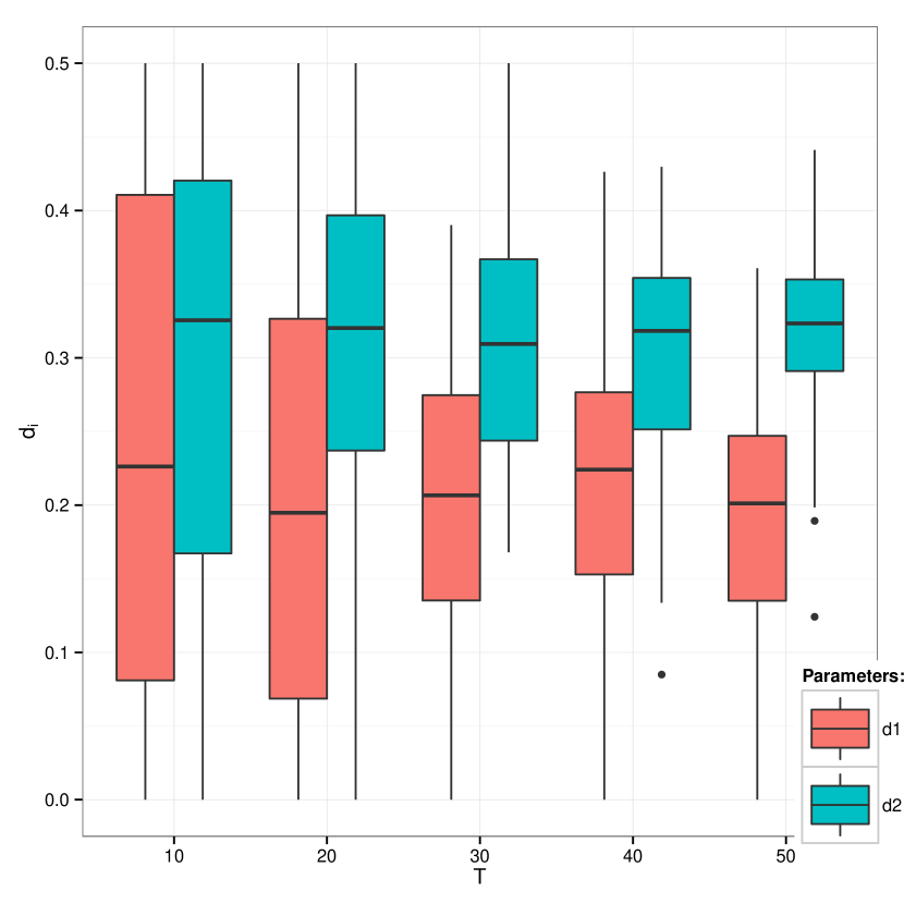
Figure 3: Boxplots of sampled values of $\hat{\boldsymbol{\theta}}_{T}.$

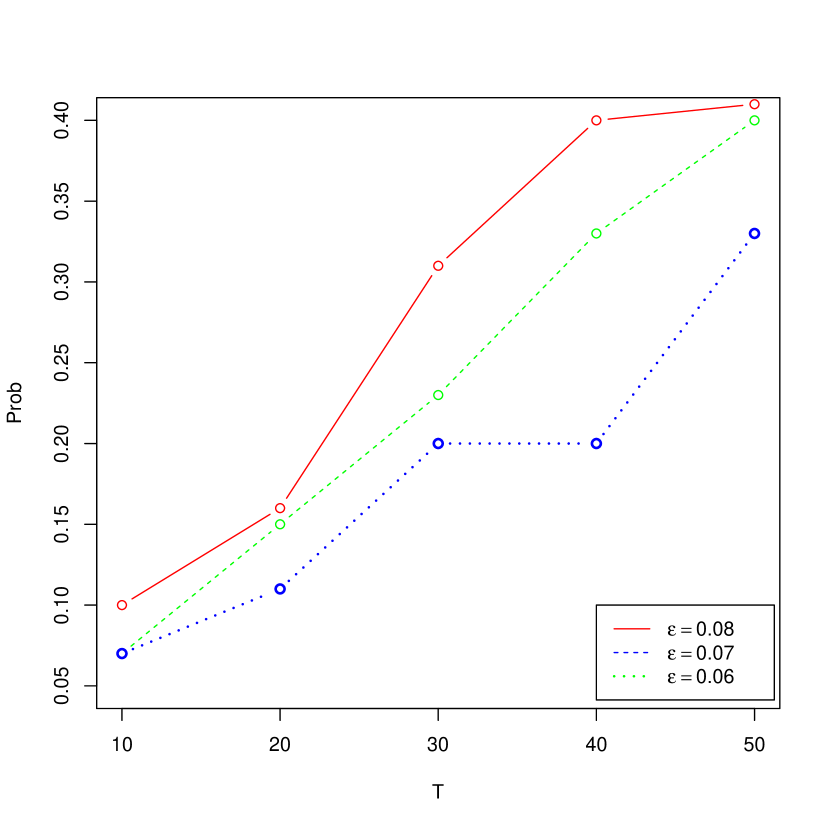
Figure 4: Sample probabilities $P_{0}(|\hat{\boldsymbol{\theta}}_{T}-{\boldsymbol{\theta}}_{0}|<\varepsilon).$

For each generated realization we also computed the value of $\hat{\sigma}^{2}_{T}$ using $I_{T}(\boldsymbol{\lambda}).$ Analogously to Figures 4, 4, plots in Figures 6, 6 support convergence in probability of $\hat{\sigma}^{2}_{T}$ to $\sigma^{2}(\boldsymbol{\theta_{0}})$ when $T$ increases. Notice that by (5) we get $\sigma^{2}(\boldsymbol{\theta_{0}})\approx 74.736$ for the selected parameters. The larger values of $\varepsilon$ in Figure 6 comparing to Figure 4 are due to the difference in the scales for the parameters (small values measured in decimals) and variances (large values measured in tens).

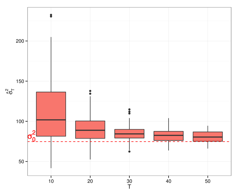
Figure 5: Boxplots of sampled values of $\hat{\sigma}^{2}_{T}.$

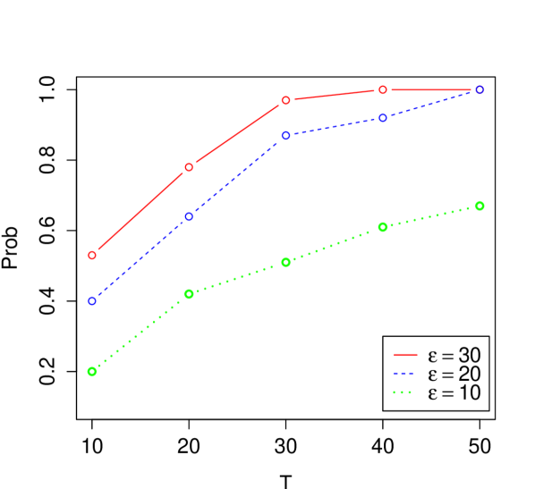
Figure 6: Sample probabilities $P_{0}(|\hat{\sigma}^{2}_{T}-\sigma^{2}(\boldsymbol{\theta_{0}})|<\varepsilon).$

To verify the result of Theorem 3.2 we used sample values $\hat{\boldsymbol{\theta}}^{*}_{50}$ which minimized the functional $\hat{U}_{T}^{*}(\boldsymbol{\theta})$ for each simulation. To avoid possible negative values the modified periodogram $I^{*}_{T}(\boldsymbol{\lambda})$ was truncated at zero by the R program. Bearing in mind the edge effect and modified periodogram’s correction, Figures 8, 8 demonstrate that the results are close to the expected ones even for the relatively small $T=50.$ The normal Q-Q plot of each component of $\hat{\boldsymbol{\theta}}_{50}^{*}$ in Figures 8 matches with the theoretical normal distribution. To test the bivariate normality hypothesis about $\hat{\boldsymbol{\theta}}_{50}^{*}$ we used the Shapiro-Wilk, energy, and kurtosis tests of multivariate normality from the R packages mvnormtest, energy, and ICS. In all the tests, p-values ($0.9491,$ $0.4605,$ and $0.5314$) confirmed that $\hat{\boldsymbol{\theta}}_{T}^{*}$ asymptotically follows a bivariate normal distribution. Simulations for other values of the parameters were run, with similar results.

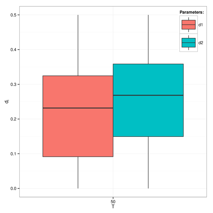
Figure 7: Boxplots of sampled values of $\hat{\boldsymbol{\theta}}_{50}^{*}.$

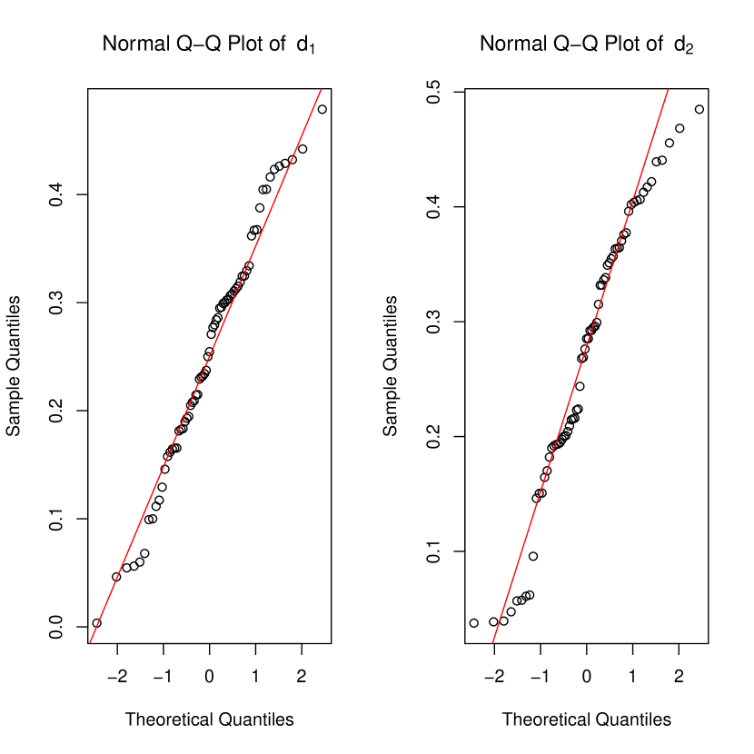
Figure 8: Normal Q-Q plots for each component of $\hat{\boldsymbol{\theta}}^{*}_{50}.$

Hence, we conclude that the MCEs are consistent estimators and the distributions of $\hat{\boldsymbol{\theta}}_{T}^{*}$ converge to the bivariate normal law. Note that the simulation studies not only comply with the obtained results for $(d_{1},d_{2})\in(0,1/4)^{2},$ but also indicate that the theoretical results may be extended to all possible values of $(d_{1},d_{2})$ in $(0,1/2)^{2}.$

6 DIRECTIONS FOR FUTURE RESEARCH

The estimation methodology based on the unbiased periodogram was introduced in Guyon [1982, 1995], see also Heyde and Gay [1993]. Recently, the paper by Robinson and Sanz [2006] and the references therein provided a detailed discussion on the topic. It studied mainly the difficulties arising in the application of the methodology in high dimensions. In particular, they investigated problems arising in relation to non-uniformly increasing domain asymptotics associated with different expansion rates of the studied domain in each spatial direction. In this paper, we considered the case $d=2$ and restricted out attention to the case of uniformly increasing domain asymptotics. The case of non-uniformly increasing domain asymptotics is left for future investigations.

An extended version of the derived results can be obtained for more general formulations of the unbiased periodogram. In particular, different growing rates can be allowed for each spatial dimension in the definition of the sampling area. For example, one can consider the following generalized version of the two-dimensional unbiased periodogram (see, for example, Robinson and Sanz [2006])

$$I_{g}(\lambda_{1},\lambda_{2})=\frac{1}{(2\pi)^{2}}\sum_{t_{1}=1-g_{1}(T)}^{g_{1}(T)-1}\sum_{t_{2}=1-g_{2}(T)}^{g_{2}(T)-1}e^{-i(\lambda_{1}t_{1}+\lambda_{2}t_{2})}\hat{\gamma}_{T}(\boldsymbol{t}),$$

where the functions $g_{i}(T),$ $i=1,2,$ satisfy some suitable conditions (for example, $g_{i}(T)\rightarrow\infty,$ $T\rightarrow\infty,$ and $g_{i}(T)\leq CT,$ $C<1,$ for $i=1,2,$ and sufficiently large $T$).

An important area for future explorations is to extend the results of Anh et al. [2004] and simultaneously estimate the locations of singularities and long-range dependence parameters using the MCE methodology. A feasible way to approach this problem would be relaxing the $L_{2}$-integrability assumptions in conditions A5-A8.

It also would be interesting to extend the methodology by Bentkus [1972] to prove the condition A9 for all $(d_{1},d_{2})$ in $(0,1/2)^{2}.$

Note that our simulation results show that the proposed minimum contrast estimation methodology works in the case of uniformly increasing domain asymptotics.

Supplementary Materials The codes used for simulations in this paper are available from the site https://googledrive.com/host/

0B7UxM8o_bnBxdG9zNU9MdHFOQUU/MCE%20Gegenbauer%20fields/

Appendix

The conditions for consistency and asymptotic normality of the MCE for parameters of stationary fractional Riesz-Bessel type random fields given in Anh et al. [2004] are specified below for random fields on $\mathbb{Z}^{2}.$

A1.

Let $Y_{t_{1},t_{2}},\ \boldsymbol{t}=(t_{1},t_{2})\in\mathbb{Z}^{2},$ be a real-valued measurable stationary Gaussian random field with zero mean and a spectral density $f(\boldsymbol{\lambda},\boldsymbol{\theta}),$ where $\boldsymbol{\lambda}=(\lambda_{1},\lambda_{2})\in[-\pi,\pi]^{2},$ $\boldsymbol{\theta}\in\Theta,$ and $\Theta$ is a compact set. Assume that $\boldsymbol{\theta}_{0}\in\mbox{int}(\Theta),$ where $\boldsymbol{\theta}_{0}$ is the true value of the parameter vector $\boldsymbol{\theta}.$

A2.

If $\boldsymbol{\theta_{1}}\neq\boldsymbol{\theta_{2}}$ then $f(\boldsymbol{\lambda},\boldsymbol{\theta_{1}})\neq f(\boldsymbol{\lambda},\boldsymbol{\theta_{2}})$ for almost all $\boldsymbol{\lambda}\in[-\pi,\pi]^{2}$ with respect to the Lebesgue measure.

A3.

There exists a nonnegative function $w(\boldsymbol{\lambda})$, $\boldsymbol{\lambda}\in[-\pi,\pi]^{2}$, such that

1. $w(\boldsymbol{\lambda})$ is symmetric about $(0,0),$ i.e. $w(\boldsymbol{\lambda})=w(-\boldsymbol{\lambda});$

2. $w(\boldsymbol{\lambda})f(\boldsymbol{\lambda},\boldsymbol{\theta})\in L_{1}\left([-\pi,\pi]^{2}\right)$ for all $\boldsymbol{\theta}\in\Theta.$

A4.

The derivatives $\nabla_{\boldsymbol{\theta}}\Psi(\boldsymbol{\lambda},\boldsymbol{\theta})$ exist and it is legitimate to differentiate under the integral sign in equation (7), i.e.

$$\nabla_{\boldsymbol{\theta}}\displaystyle\int_{[-\pi,\pi]^{2}}\Psi(\boldsymbol{\lambda},\boldsymbol{\theta})w(\boldsymbol{\lambda})\,\,d\boldsymbol{\lambda}=\displaystyle\int_{[-\pi,\pi]^{2}}\nabla_{\boldsymbol{\theta}}\Psi(\boldsymbol{\lambda},\boldsymbol{\theta})w(\boldsymbol{\lambda})\,\,d\boldsymbol{\lambda}=0.$$

A5.

For all $\boldsymbol{\theta}\in\Theta$ the function $w(\boldsymbol{\lambda})$, $\boldsymbol{\lambda}\in[-\pi,\pi]^{2},$ satisfies

$$f(\boldsymbol{\lambda},\boldsymbol{\theta_{0}})w(\boldsymbol{\lambda})\log\Psi(\boldsymbol{\lambda},\boldsymbol{\theta})\in L_{1}\left([-\pi,\pi]^{2}\right)\cap L_{2}\left([-\pi,\pi]^{2}\right).$$

A6.

There exists a function $\upsilon(\boldsymbol{\lambda}),$ $\boldsymbol{\lambda}\in[-\pi,\pi]^{2},$ such that

1. the function $h(\boldsymbol{\lambda},\boldsymbol{\theta})=\upsilon(\boldsymbol{\lambda})\log\Psi(\boldsymbol{\lambda},\boldsymbol{\theta})$ is uniformly continuous on $[-\pi,\pi]^{2}\times\Theta;$

2. $f(\boldsymbol{\lambda},\boldsymbol{\theta}_{0})w(\boldsymbol{\lambda})/\upsilon(\boldsymbol{\lambda})\in L_{1}([-\pi,\pi]^{2})\cap L_{2}([-\pi,\pi]^{2}).$

A7.

The function $\Psi(\boldsymbol{\lambda},\boldsymbol{\theta})$ is twice differentiable on $\Theta$ and

1. $f(\boldsymbol{\lambda},\boldsymbol{\theta}_{0})w(\boldsymbol{\lambda})\frac{\partial^{2}}{\partial\theta_{i}\partial\theta_{j}}\log\Psi(\boldsymbol{\lambda},\boldsymbol{\theta})\in L_{1}([-\pi,\pi]^{2})\bigcap L_{2}([-\pi,\pi]^{2}),$ for all $i,j,$ and $\boldsymbol{\theta}\in\Theta;$

2. $f(\boldsymbol{\lambda},\boldsymbol{\theta}_{0})w(\boldsymbol{\lambda})\frac{\partial}{\partial\theta_{i}}\log\Psi(\boldsymbol{\lambda},\boldsymbol{\theta})\in L_{k}([-\pi,\pi]^{2}),$ for all $i,$ $\boldsymbol{\theta}\in\Theta,$ and $k\geq 1.$

A8.

The matrices $\mathbf{S}(\boldsymbol{\theta})=(s_{ij}(\boldsymbol{\theta}))$ and $\mathbf{A}(\boldsymbol{\theta})=(a_{ij}(\boldsymbol{\theta}))$ with the elements defined by (11) and (12) are positive definite.

A9.

The spectral density $f(\boldsymbol{\lambda},\boldsymbol{\theta}),$ the weight function $w(\boldsymbol{\lambda}),$ and the function $\frac{\partial}{\partial\theta_{i}}\log\Psi(\boldsymbol{\lambda},\boldsymbol{\theta})$ are such that for all $i$ and $\boldsymbol{\theta}\in\Theta:$

$$T\displaystyle\int_{[-\pi,\pi]^{2}}(EI^{*}_{T}(\boldsymbol{\lambda})-f(\boldsymbol{\lambda},\boldsymbol{\theta}_{0}))w(\boldsymbol{\lambda})\frac{\partial}{\partial\theta_{i}}\log\Psi(\boldsymbol{\lambda},\boldsymbol{\theta})\,\,d\boldsymbol{\lambda}\longrightarrow 0,\quad\text{as}\quad T\longrightarrow\infty.$$

References

• Abramowitz and Stegun [1972] Abramowitz M, Stegun IA, eds. (1972) Handbook of mathematical functions with formulas, graphs, and mathematical tables. Dover, New York
• Anh et al. [1999] Anh VV, Angulo JM, Ruiz-Medina MD (1999) Possible long-range dependence in fractional random fields. J Stat Plan Infer 80:95–110
• Anh et al. [2004] Anh VV, Leonenko NN, Sakhno LM (2004) On a class of minimum contrast estimators for fractional stochastic processes and fields. J Stat Plan Infer 123:161–185
• Anh et al. [2007] Anh VV, Leonenko NN, Sakhno LM (2007) Minimum contrast estimation of random processes based on information of second and third orders. J Stat Plan Infer 137(4):1302–1331
• Anh and Lunney [1995] Anh VV, Lunney KE (1995) Parameter estimation of random fields with long-range depedence. Math Comput Model 21:67–77
• Arteche and Robinson [2000] Arteche J, Robinson PM (2000) Semiparametric inference in seasonal and cyclical long memory processes. J Time Ser Anal 21(1):1–25
• Basu and Reinsel [1993] Basu S, Reinsel GC (1993) Properties of the spatial unilateral first-order $ARMA$ model. Adv Appl Probab 25(3):631–648
• Bentkus [1972] Bentkus R (1972) The error in estimating the spectral function of a stationary process. Litovsk Mat Sb 12(1):55–71
• Beran et al. [2009] Beran J, Ghosh S, Schell D (2009) On least squares estimation for long-memory lattice processes. J Multivariate Anal 100:2178–2194
• Boissy et al. [2005] Boissy Y, Bhattacharyya BB, Li X, Richardson GD (2005) Parameter estimates for fractional autoregressive spatial process. Ann Statist 33:2553–2567
• Brychkov et al. [1992] Brychkov YuA, Glaeske HJ, Prudnikov AP, Vũ KT (1992) Multidimensional integral transformations. Gordon and Breach Science Publishers, New York
• Chan and Tsai [2012] Chan KS, Tsai H (2012) Inference of seasonal long-memory aggregate time series. Bernoulli 4(18):1448–1464
• Chung [1996a] Chung CF (1996) A generalized fractionally integrated autoregressive moving-average process. J Time Ser Anal 17:111–140
• Chung [1996b] Chung CF (1996) Estimating a generalized long memory process. J Econometrics 73:237–259
• Cohen and Francos [2002] Cohen G, Francos JM (2002) Linear least squares estimation of regression models for two-dimensional random fields. J Multivariate Anal 82:431–444
• Collet and Fadili [2006] Collet JJ and Fadili MJ (2006) Simulation of Gegenbauer Processes using Wavelet Packets. arXiv:math/0608613
• Espejo et al. [2014] Espejo RM, Leonenko N, Ruiz-Medina MD (2014) Gegenbauer random fields. Random Oper Stoch Equ 22(1): 1–16