Modularity Enhances the Rate of Evolution in a Rugged Fitness Landscape

Abstract

Biological systems are modular, and this modularity affects the evolution of biological systems over time and in different environments. We here develop a theory for the dynamics of evolution in a rugged, modular fitness landscape. We show analytically how horizontal gene transfer couples to the modularity in the system and leads to more rapid rates of evolution at short times. The model, in general, analytically demonstrates a selective pressure for the prevalence of modularity in biology. We use this model to show how the evolution of the influenza virus is affected by the modularity of the proteins that are recognized by the human immune system. Approximately 25% of the observed rate of fitness increase of the virus could be ascribed to a modular viral landscape.

1 Introduction

Biological systems are modular, and the organization of their genetic material reflects this modularity [1, 2, 3, 4]. Complementary to this modularity is a set of evolutionary dynamics that evolves the genetic material of biological systems. In particular, horizontal gene transfer (HGT) is an important mechanism of evolution, in which genes, pieces of genes, or multiple genes are transferred from one individual to another [5, 6, 7]. Additionally, multi-body contributions to the fitness function in biology are increasingly thought to be an important factor in evolution [8], leading to a rugged fitness landscape and glassy evolutionary dynamics. The combination of modularity and horizontal gene transfer provide an effective mechanism for evolution upon a rugged fitness landscape [9]. The organization of biology into modules simultaneously restricts the possibilities for function, because the modular organization is a subset of all possible organizations, and may lead to more rapid evolution, because the evolution occurs in a vastly restricted modular subspace of all possibilities [9, 10]. Our results explicitly demonstrate this trade off, with $t^{*}$ serving as the crossover time from the latter to the former regime.

Thus, the fitness function in biology is increasingly realized to be rugged, yet modular. Nonetheless, nearly all analytical theoretical treatments assume a smooth fitness landscape with a dependence only on Hamming distance from a most-fit sequence [11], a linear or multiplicative fitness landscape for dynamical analysis of horizontal gene transfer [12, 13], or an uncorrelated random energy model [14, 15]. Horizontal gene transfer processes on more general, but still smooth, landscapes have been analyzed [16, 17, 18, 19, 20]. Here we provide, to our knowledge, the first analytical treatment of a finite-population Markov model of evolution showing how horizontal gene transfer couples to modularity in the fitness landscape. We prove analytically that modularity can enhance the rate of evolution for rugged fitness landscapes in the presence of horizontal gene transfer. This foundational result in the physics of biological evolution offers a clue to why biology is so modular. We demonstrate this theory with an application to evolution of the influenza virus.

We introduce and solve a model of individuals evolving on a modular, rugged fitness landscape. The model is constructed to represent several fundamental aspects of biological evolution: a finite population, mutation and horizontal gene transfer, and a rugged fitness landscape. For this model, we will show that the evolved fitness is greater for a modular landscape than for a non-modular landscape. This result holds for $t<t^{*}$ where $t^{*}$ is a crossover time, larger than typical biological timescales. The dependence of the evolved fitness on modularity is multiplicative with the horizontal gene transfer rate, and the advantage of modularity disappears when horizontal gene transfer is not allowed. Our results describe the response of the system to environmental change. In particular, we show that modularity allows the system to recover more rapidly from change, and fitness values attained during the evolved response to change increase with modularity for large or rapid environmental change.

2 Theory of the Rate of Evolution in a Rugged Fitness Landscape

We use a Markov model to describe the evolutionary process. There are $N$ individuals. Each individual $\alpha$ replicates at a rate $f_{\alpha}$. The average fitness in the population is defined as $\langle f\rangle=\frac{1}{N}\sum_{\alpha=1}^{N}f_{\alpha}$. Each individual has a sequence $S^{\alpha}$ that is composed of $L$ loci, $s_{i}^{\alpha}$. For simplicity, we take $s_{i}^{\alpha}=\pm 1$. Each of the loci can mutate to the opposite state with rate $\mu$. Each sequence is composed of $K$ modules of length $l=L/K$. A horizontal gene transfer process randomly replaces the $k$th module in the sequence of individual $\alpha$, e.g. the sequence loci $s_{(k-1)l+1}^{\alpha}\ldots s_{kl}^{\alpha}$, with the corresponding sequences from a randomly chosen individual $\beta$ at rate $\nu$. The a priori rate of sequence change in a population is, therefore, $N\mu L$ + $N\nu L/2$. Since the fitness landscape in biology is rugged, we use a spin glass to represent the fitness:

$$f[S] = 2L+H[S]$$

$$H[S] = \sum_{ij}s_{i}s_{j}J_{ij}\Delta_{ij}$$ (1)

$J_{ij}$ is a quenched, Gaussian random matrix, with variance $1/C$. As discussed in Appendix A, the offset value $2L$ is chosen by Wigner’s semicircle law so that the minimum eigenvalue of $f$ is non-negative. The entries in the matrix $\Delta$ are zero or one, with probability $C/L$ per entry, so that the average number of connections per row is $C$. We introduce modularity by an excess of interactions in $\Delta$ along the $l\times l$ block diagonals of the $L\times L$ connection matrix. There are $K$ of these block diagonals. Thus, the probability of a connection is $C_{0}/L$ when $\lfloor i/l\rfloor\neq\lfloor j/l\rfloor$ and $C_{1}/L$ when $\lfloor i/l\rfloor=\lfloor j/l\rfloor$. The number of connections is $C=C_{0}+(C_{1}-C_{0})/K$. Modularity is defined by $M=(C_{1}-C_{0})/(KC)$ and obeys $-1/(K-1)\leq M\leq 1$.

The Markov process describing these evolutionary dynamics includes terms for replication ($f$), mutation ($\mu$), and horizontal gene transfer ($\nu$):

$$\frac{dP(\{n_{\bf a}\};t)}{dt} = \sum_{\{{\bf a}\}}\bigg{[}f(S_{\bf a})(n_{\bf a}-1)\sum_{\{{\bf b}\neq{\bf a}\}}\frac{n_{\bf b}+1}{N}P(n_{\bf a}-1,n_{\bf b}+1;t)-f(S_{\bf a})n_{\bf a}\sum_{\{{\bf b}\neq{\bf a}\}}\frac{n_{\bf b}}{N}P(n_{\bf a},n_{\bf b};t)\bigg{]}$$

$$+\mu\sum_{\{{\bf a}\}}\sum_{\{{\bf b}=\partial{\bf a}\}}\bigg{[}(n_{\bf b}+1)P(n_{\bf a}-1,n_{\bf b}+1;t)-n_{\bf b}P(n_{\bf a},n_{\bf b};t)\bigg{]}$$

$$+\nu\sum_{\{{\bf a}\}}\sum_{k=1}^{K}\sum_{\{{\bf b},{\bf b}_{k}\neq{\bf a}_{k}\}}\bigg{[}(n_{{\bf a}/{\bf b}_{k}}+1)\frac{n_{{\bf b}/{\bf a}_{k}}}{N}P(n_{\bf a}-1,n_{{\bf a}/{\bf b}_{k}}+1;t)$$

$$-n_{{\bf a}/{\bf b}_{k}}\frac{n_{{\bf b}/{\bf a}_{k}}}{N}P(n_{\bf a},n_{{\bf a}/{\bf b}_{k}};t)\bigg{]}$$

Here $n_{\bf a}$ is the number of individuals with sequence $S_{\bf a}$, with the vector index ${\bf a}$ used to label the $2^{L}$ sequences. This process conserves $N=\sum_{\bf a}n_{\bf a}$. The notation $\partial{\bf a}$ means the $L$ sequences created by a single mutation from sequence $S_{\bf a}$. The notation ${\bf a}/{\bf b}_{k}$ means the sequence created by horizontally gene transferring module $k$ from sequence $S_{\bf b}$ into sequence $S_{\bf a}$.

We consider how a population of initially random sequences adapts to a given environment, averaged over the distribution of potential environments. For example, in the context of influenza evolution, these sequences arise, essentially randomly, by transmission from swine. As discussed in Appendix B, a short-time expansion for the average fitness can be derived by recursive application of this master equation:

$$\langle f(t)\rangle = 2L+at+bt^{2}$$

$$a = 2L\left(1-\frac{1}{N}\right)$$

$$b = -\frac{4L^{2}}{N}\left(1-\frac{1}{N}\right)-4\mu L\left(1-\frac{1}{N}\right)$$ (3)

$$-2\nu L\left[\left(1-\frac{1}{K}\right)\left(1-M\right)\left(1-\frac{4}{N}\right)+\frac{1}{N}\right]\left(1-\frac{1}{N}\right)$$

Result (3) is exact for all finite $N$. Note that the effect of modularity enters at the quadratic level and requires a non-zero rate of horizontal gene transfer, $\nu>0$. We see that $\langle f_{M>0}(t)\rangle>\langle f_{0}(t)\rangle$ for short times.

From the master equation, we also calculate the sequence divergence, defined as $D=\frac{1}{N}\sum_{\alpha=1}^{N}\langle\frac{L-S_{\alpha}(t)\cdot S_{\alpha}(0)}{2}\rangle$. As discussed in Appendix C, recursive application of Eq. (LABEL:2) gives

$$D = \alpha t+\beta t^{2}$$

$$\alpha = L^{2}\left(1-\frac{1}{N}\right)+\mu L+\frac{\nu L}{2}\left(1-\frac{1}{N}\right)$$

$$\beta = -L^{3}\left(1-\frac{1}{2L}+\frac{3}{2LN}\right)\left(1-\frac{1}{N}\right)-2\mu L^{2}\left(1-\frac{1}{N}\right)-\nu L^{2}\left(1-\frac{1}{N}\right)$$ (4)

$$-\mu^{2}L-\mu\nu L\left(1-\frac{1}{N}\right)-\frac{1}{4}\nu^{2}L\left(1-\frac{1}{N}\right)$$

The sequence divergence does not depend on modularity at second order in time. Note the terms at order $t^{n}$ not proportional $\mu^{m}\nu^{n-m}$ are due to discontinuous changes in sequence resulting from the fixed population size constraint.

Introduction of a new sequence into an empty niche corresponds to an initial condition of identical, rather than random, sequences. The population dynamics again follows Eq. (LABEL:2). To see an effect of modularity, an expansion to 4th order in time is required. As discussed in Appendix B, we find

$$\langle f(t)\rangle=2L+bt^{2}+ct^{3}+dt^{4}$$ (5)

with

$$(2!)b = 16\mu L(1-1/N)$$

$$(3!)c = -64\mu L^{2}(1-1/N)/N-192\mu^{2}L(1-1/N)-32\mu\nu L(1-1/N)/N$$

$$(4!)d = 128\mu^{2}\nu LM(1-1/K)(1-1/N)(1-4/N)+64\mu L(1-1/N)[2(6+14\mu^{2}-\mu\nu)$$

$$+2\mu\nu(1-4/N)/K-2(36-10\mu L-9\mu\nu)/N+(4L^{2}+2L+92+4\nu L+\nu^{2})/N^{2}]$$

Interestingly, the fitness function initially increases quadratically. The modularity dependence enters at fourth order, and $\langle f_{M>0}(t)\rangle>\langle f_{0}(t)\rangle$ for short times.

3 Comparison of Theory to Simulation Results

The response function of the modular and non-modular system can be computed numerically as well. We start the system off with random initial sequences, so that the average initial $\langle f(0)\rangle-2L$ is zero, and compute the evolution of the average fitness, $\langle f(t)\rangle$. In Fig. 1 we show the results from a Lebowitz-Gillespie simulation. We see that $\langle f_{M}(t)\rangle>\langle f_{0}(t)\rangle$ for $t<t^{*}$ for $M=1$. That is, the modular system evolves more quickly to improve the average fitness, for times less than a crossover time, $t^{*}$. For $t>t^{*}$, the constraint that modularity imposes on the connections leads to the non-modular system dominating, $\langle f_{0}(t)\rangle>\langle f_{M}(t)\rangle$.

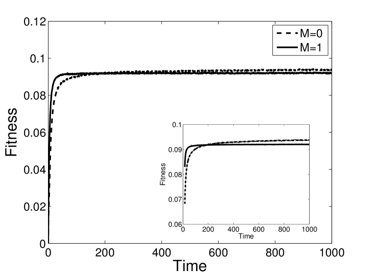
Figure 1: Shown is the population average fitness for the modular ($M=1$, solid) and non-modular ($M=0$, dashed) systems. Fitness is normalized by $L$ and the offset $2L$ is subtracted. The modular system evolves to a greater fitness value for times $t<t^{*}$. Here $t^{*}\approx 182$. Here Eq. (1) has been scaled by $\epsilon=0.1$, and $L=100$, $N=10000$, $\mu=0.05$, $\nu=0.6$, $K=5$, and $C=L/K-1$, motivated by application to evolution of influenza to be discussed below. In inset is shown the fit of the data to the form of Eq. (7).

Eq. (3) shows these results analytically, and we have checked Eq. (3) by numerical simulation as well. For the parameter values of Fig. 1 and $M=0$, theory predicts $a/L=0.019998$, $b/L=-0.011636$, and simulation results give $a/L=0.020529\pm 0.000173$, $b/L=-0.011306\pm 0.000406$. For $M=1$, theory predicts $a/L=0.019998$, $b/L=-0.002041$, and simulation results give $a/L-0.019822\pm 0.000200$, $b/L=-0.0019084\pm 0.000177$

Since the landscape is rugged, we expect the time it takes the system to reach a given fitness value, $\langle f(t)\rangle$, starting from random sequences to grow in a stretched exponential way at large times. Moreover, since the combination of horizontal gene transfer and modularity improves the response function at short times, we expect that the difference in times required to reach $\langle f(t)\rangle$ of a non-modular and modular system also increases in a stretched exponential way, by analogy with statistical mechanics, in which we expect the spin glass energy response function to converge as

$$\langle f(t)\rangle\sim f_{\infty}-c\ln^{-2/\nu}t/t_{0}$$ (7)

with $\nu=1$ [21]. Figure 1 shows the fit of the data to this functional form, with $f_{\infty}=0.958$, $c=0.067$, $t_{0}=3.168$ for $M=0$ and $f_{\infty}=0.922$, $c=0.004$, $t_{0}=7.619$ for $M=1$. Figure 2 shows the stretched exponential speedup in the rate of evolution that modularity provides.

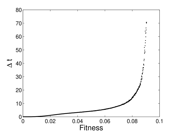
Figure 2: Shown is the difference in time required, $\Delta t$, for the modular ($M=1$) and non-modular ($M=0$) system to reach a specified average fitness value for times $t<t^{*}$, starting from random initial sequences. Parameter values are as in Fig. 1.

The prediction for evolution of a population of identical sequences in a new niche is shown in Eq. (LABEL:101). Analytically, the effect of modularity shows up at 4th order rather than 2nd order when all sequences are initially identical. Qualitatively, however, at all but the very shortest times, the results for random and identical sequences are similar, as shown in Figs. 1 and 3.

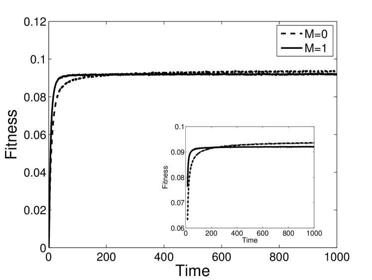
Figure 3: Shown is the population average fitness for the modular ($M=1$, solid) and non-modular ($M=0$, dashed) systems when all individuals initially have the same sequence. Fitness is normalized by $L$ and the offset $2L$ is subtracted. The modular system evolves to a greater fitness value for times $t<t^{*}$. Here $t^{*}\approx 230$. Parameter values are as in Fig. 1.

4 Average Fitness in a Changing Environment

We show how to use these results to calculate the average fitness in a changing environment. We consider that every $T$ time steps, the environment randomly changes. During such an environmental change, each $J_{ij}$ in the fitness, Eq. (1), is randomly redrawn from the Gaussian distribution with probability $p$. That is, on average, a fraction $p$ of the fitness is randomized. Due to this randomization, the fitness immediately after the environmental change will be $1-p$ times the value immediately before the change, on average. This condition allows us to calculate the average time-dependent fitness during evolution in one environment as a function of $p$ and $T$, given only the average fitness starting from random initial conditions, $\langle f(t)\rangle$ [22]. We denote the average fitness reached during evolution in one environment as $f_{p,T}(M)$. This is related to the average fitness with random initial conditions by $f_{p,T}(M)=\langle f(M)\rangle(t)$, where $t$ is chosen to satisfy $\langle f(M)\rangle(t-T)=(1-p)\langle f(M)\rangle(t)$ due to the above condition. Thus, for high rates or large magnitudes of environmental change, Eq. (3) can be directly used along with these two conditions to predict the steady-state average population fitness.

a) b)

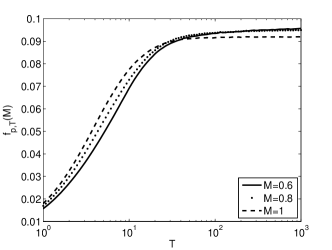
c)

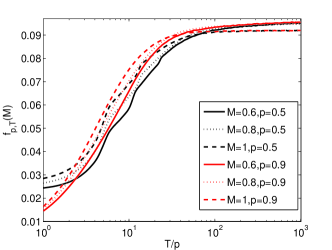
Figure 4: Shown is the fitness, $f_{p,T}(M)$, in an environment that changes with characteristic time $T$ and magnitude a) $p=0.5$ or b) $p=0.9$. c) The fitness is replotted as a function of T/p. For each $p$, the fitness is shown for three values of modularity: $M=0.6$ (solid), $M=0.8$ (dotted), and $M=1$ (dashed). Parameters are as in Fig. 1.

Figure 4 shows how the average fitness depends on the rate and magnitude of environmental change. The average fitness values for a given modularity are computed numerically. The figure displays a crossing of the modularity-dependent fitness curves. The curve associated with the largest modularity is greatest at short times. There is a crossing to the curve associated with the second largest modularity at intermediate times. And there is a crossing to the curve associated with the smallest modularity at somewhat longer times. In other words, the value of modularity that leads to the highest average fitness depends on time, $T$, decreasing with increasing time.

Figure 4 demonstrates that larger values of modularity, greater $M$, lead to higher average fitness values for faster rates of environmental change, smaller $T$. The advantage of greater modularity persists to larger $T$ for greater magnitudes of environmental change, larger $p$. In other words, modularity leads to greater average fitness values either for greater frequencies of environmental change, $1/T$, or greater magnitudes of environmental change, $p$.

It has been argued that an approximate measure of the environmental pressure is given by the product of the magnitude and frequency of environmental change $p/T$ [22]. If this is the case, then the curves in Fig.  4ab as a function of $T$ for different values of $p$ should collapse to a single curve as a function of $T/p$. As shown in Fig.  4c, this is approximately true for the three cases $M=0.6$, $M=0.8$, and $M=1$.

5 Application of Theory to Influenza Evolution Data

We here apply our theory to the evolution of the influenza virus. Influenza is an RNA virus of the Orthomyxoviridae family. The 11 proteins of the virus are encoded by 8 gene segments. Reassortment of these gene segments is common [23, 24, 25]. In addition, there is a constant source of genetic diveristy, as most human influenza viruses arise from birds, mix in pigs, with a select few transmitted to humans [23, 24, 25, 26]. We model a simplification of this complex coevolutionary dynamics with the theory presented here. We consider $K\approx 5$ modules, with mutations in the genetic material encoding them leading to an effective mutation rate at the coarse-grained length scale. We do not consider individual amino acids, but rather a coarse-grained $L=100$ reprsentation the viral protein material. The virus is under strong selective pressure to adapt to the human host, having most often arisn in birds and trasmitted through swine. The virus is also under strong pressure from the human immune system. The virus evolves in response to this pressure, thereby increasing its fitness. The increase in fitness was estimated by tracking the increase in frequency of each viral strain, as observed in the public sequence databases: $\ln[f_{i}(t+1)/f_{i}(t)]=\hat{x}_{i}(t+1)/x_{i}(t)$, where $f_{i}(t)$ is the fitness of clade $i$ at time $t$, $x_{i}(t)$ is the frequency of clade $i$ among all clades observed at time $t$, and $\hat{x}_{i}(t+1)$ is the frequency at $t+1$ predicted by a model that includes a description of the mutational processes [27]. Here “clade” is a term for the quasispecies of closely-related influenza sequences at time $t$. We use these approximate fitness values, estimated from observed HA sequence patterns and an approximate point mutation model of evolution, for comparison to the present model.

Influenza evolves within a cluster of closely-related sequences for 3–5 years and then jumps to a new cluster [28, 29, 30]. Indeed, the fitness flux data over 17 years [27] shows a pattern of discontinuous changes every 3–5 years. Often these jumps are related to influx of genetic material from swine [23, 24, 25, 26]. By clustering the strains, the clusters and the transitions between them can be identified: the flu strain evolved from Wuhan/359/95 to Sydney/5/97 at 1996-1997, Panama/2007/1999 to Fujian/411/2002 at 2001-2002, California/7/2004 to Wisconsin/67/2005 at 2006-2007, Brisbane/10/2007 to BritishColumbia/RV1222/09 at 2009-2010 [30]. These cluster transitions correspond to the discontinuous jumps in the fitness flux evolution and discontinuous changes in the sequences. Our theory represents the evolution within one of these clusters, considering reassortment only among human viruses. Thus, we predict the evolution of the fitness during each of these periods. There are 4 periods within the time frame 1993–2009. Figure 5 shows the measured fitness data [27], averaged over these four time periods.

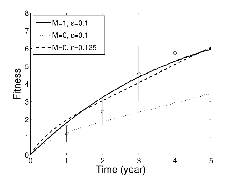
Figure 5: Shown is the fitness of influenza virus H3N2 in humans, estimated from the time derivative of the frequency with which sequences appear in the GenBank sequence database. Each time a new circulating strain is introduced to humans, typically from pigs infected from birds, the fitness increases as a quasispecies expands around the strain. The average fitness increase over four such antigenic shifts between 1993 and 2010 is shown. Data are from [27]. Error bars are one standard error. Theoretical results are shown for the modular ($M=1$, solid) and non-modular ($M=0$, dotted) model predictions. Theory was fit to the average linear fitness increase at 5 years. Parameter values are as in Fig. 1, with fitness scaled by $\epsilon=0.1$. Theoretical results are also shown for $\epsilon=0.125$ and $M=0$ (dashed).

We scaled Eq. (1) by $\epsilon$ to fit the observed data. The predictions from Eq. (3) are shown in Fig. 5. We find $\epsilon=0.1$ and $M=1$ fit the observed data well. We assume the overall rate of evolution is equally contributed to by mutation and horizontal gene transfer. The average observed substitution rate in the 100aa epitope region of the HA protein is 5 amino acids per year [30, 27]. We interpret this result in our coarse-grained model to imply $\mu=.05$ and $\nu=0.6$.

The value of $\epsilon$ required to fit the non-modular model to the data is 25% greater than the value required to fit the modular model to the data. That is, approximately 25% of the observed rate of fitness increase of the virus could be ascribed to a modular viral fitness landscape. Thus, to achieve the observed rate of evolution, the virus may either have evolved modularity $M=1$, or the virus may have evolved a 25% increase in its replication rate by other evolutionary mechanisms. Given the modular structure of the epitopes on the haemagglutinin protein of the virus, the modular nature of the viral segments, and the modular nature of naive, B cell, and T cell immune responses we suggest that influenza has likely evolved a modular fitness landscape.

6 Generalization to Investigate the Effect of Landscape Ruggedness

We here generalize Eq. (1) to $p$-spin interactions, $q$ letters in the alphabet from which the sequences are constructed, and what is known as the GNK random matrix form of interactions [31]. These generalizations allow us to investigate the effect of landscape ruggedness on the rate of evolution.

6.1 Generalization to the $p$-spin SK Model

We first generalize the SK model to interactions among $p$ spins, which we term the $p$SK model. The $p$SK landscape is more rugged for increasing $p$. Thus, we might expect modularity to play a more important role for the models with larger $p$. The generalized fitness is written as

$$f=\sum_{i_{1}i_{2}...i_{p}}J_{i_{1}i_{2}...i_{p}}\Delta_{i_{1}i_{2}...i_{p}}s_{i_{1}}s_{i_{2}}...s_{i_{p}}+2L$$ (8)

The $J$ and $\Delta$ tensors are symmetric, that is, $J_{i_{1}i_{2}...i_{p}}=J_{[i_{1}i_{2}...i_{p}]}$ and $\Delta_{i_{1}i_{2}...i_{p}}=\Delta_{[i_{1}i_{2}...i_{p}]}$, where $[i_{1}i_{2}...i_{p}]$ is any permutation of $i_{1}i_{2}...i_{p}$. The probability of a connection is $C_{1}/L^{p-1}$ inside the block, $\lfloor i_{1}/l\rfloor=\lfloor i_{2}/l\rfloor=...=\lfloor i_{p}/l\rfloor$, and $C_{0}/L^{p-1}$ outside the blocks. The connections are defined as

$$\sum_{i_{2}...i_{p}}\Delta_{i_{1}i_{2}...i_{p}}=C$$ (9)

Since $C=C_{0}[1-(\frac{1}{K})^{p-1}]+C_{1}(\frac{1}{K})^{p-1}$, it follows that $C_{1}=C[MK^{p-1}+(1-M)]$, and $C_{0}=C(1-M)$.

Increasing the value of $p$ makes the landscape more rugged, and so it is more difficult for system to reach a given value of the fitness in a finite time. Thus, modularity is expected to play a more significant role in giving the system an evolutionary advantage. Specifically we expect that the effect of modularity will show up at shorter times for larger $p$. As shown in Appendix B, we find

$$a = 2L(1-1/N)$$

$$2b = -\frac{8L^{2}}{N}(1-1/N)-4\mu pL(1-1/N)$$ (10)

$$+2\nu L\left[\left(\frac{2}{N}-p+\frac{3p}{N}\right)(1-M)\left(1-\frac{1}{K^{p-1}}\right)-\frac{2}{N}\right](1-1/N)$$

The modular terms increase faster with $p$ than the non-modular terms, so the dependence on modularity of evolution is more significant with bigger $p$. Figure 6 shows the average fitness curves for the $p$-spin interaction. Due to the normalization of the $J$ values, all fitness curves have the same slope at $t=0$, i.e. the same values of $a$. However, increasing $p$ leads to slower rates of fitness increase at finite time, especially for the $M=0$ case. At finite time, for large values of $p$, the evolutionary advantage of larger $M$ is more pronounced. That is, modularity help the sequences to evolve more efficiently.

Figure 6: Results for $2$-spin, $12$-spin and $30$-spin SK interaction fitness when initial sequences are random. The fitness is given by Eq. (8). The parameters are as in Fig. 1.

We also calculated the average fitness for the initial condition of all sequences identical. As discussed above, many-spin effects make the landscape more rugged for larger $p$. We seek to understand this effect quantitatively for the case of same initial sequences as well. As shown in Appendix B, the Taylor expansion results are

$$(2!)b = 8\mu pL(1-1/N)$$

$$(3!)c = -32\mu pL^{2}(1-1/N)/N-16\mu^{2}p^{2}L(1-1/N)$$

$$-64\mu^{2}pL(1-1/N)-16\mu\nu pL(1-1/N)/N$$

$$(4!)d = 64\mu^{2}\nu p(p-1)LM(1-1/K)(1-1/N)(1-4/N)$$

$$+32\mu pL(1-1/N)[(6p+7\mu^{2}p^{2}-2\mu\nu(p-1))$$

$$+2\mu\nu(1-4/N)/K-(36p-10\mu pL-5\mu\nu p-8\mu\nu(p-1))/N$$

$$+(4L^{2}+2L+46p+4\nu L+\nu^{2})/N^{2}]$$

6.2 Generalization to the Planar Potts Model

We here generalize the alphabet from two-states, $s_{i}=\pm 1$, to $q$ states, with a planar Potts model [32] of the fitness. The $q=2$ model is often justified as a projection of the $q=4$ nucleic acid alphabet onto purines and pyrimidines. Thus, $q=4$ is a relevant generalization. Additional $q=20$ corresponds to the amino acid alphabet. The alphabet size can affect the evolutionary phase diagram [33], so $q$ is a relevant order parameter. In the planar Potts model, each vector spin takes on $q$ equidistant angles, and the angle between two is defined by $\boldsymbol{s}_{i}\cdot\boldsymbol{s}_{j}=\cos\theta_{ij}$. The fitness is

$$f=\sum_{ij}J_{ij}\Delta_{ij}\cos\theta_{ij}+2L$$ (12)

The directions of a spin are evenly spaced in the plane, so when the spin points to $q$ directions, the angle between two spins is $2k\pi/q$, where $k$ can be $0$, $1$, …, $q-1$.

The evolutionary dynamics in the planar Potts model is distinct from that in the $p$SK model. As shown in Appendix B,

$$a = L(1-1/N)(1+\delta_{q,2})$$

$$2b = -4L^{2}(1-1/N)(1+\delta_{q,2})/N-2\mu L(1-1/N)\frac{q}{q-1}(1+\delta_{q,2})$$ (13)

$$-2\nu L\left[\left(1-\frac{1}{K}\right)\left(1-M\right)\left(1-\frac{4}{N}\right)+\frac{1}{N}\right]\left(1-\frac{1}{N}\right)(1+\delta_{q,2})$$

Figure 7 displays results for two values of $q$. Increasing $q$ does increase the landscape ruggedness in the planar Potts model. There is an evolutionary speedup provided by modularity. The $q$ dependence, however, is not as dramatic as in the $p$SK model.

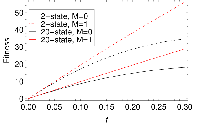
Figure 7: Average fitness in the planar Potts model for alphabet sizes of $q=2$ or $q=20$. Sequences are initially random. The fitness Eq.  (12). Other parameters are same as in Fig. 1.

6.3 Generalization to the GNK Model

A model related to the SK form is the GNK model, a simple form of which is

$$f=H+2L=\sum_{ij}\sigma_{ij}(s_{i},s_{j})\Delta_{ij}+2L$$ (14)

where the $\sigma$ matrix is a symmetric matrix with random Gaussian entries, and the $\Delta$ matrix is the same as that in Eq. (1). Other than the condition of symmetry, the entries in the $\sigma$ matrices are independently drawn from a Gaussian distribution of zero mean and unit variance in each matrix and for different $i,j$. Thus, other than the condition $\sigma_{ij}=\sigma{ji}$, the values are independent for different $i$, $j$, $s_{i}$, or $s_{j}$. This form is generalized to a $p$-spin, $q$-state form as

$$f=\sum_{i_{1}i_{2}...i_{p}}\sigma_{i_{1}i_{2}...i_{p}}(s_{i_{1}},s_{i_{2}},...,s_{i_{p}})\Delta_{i_{1}i_{2}...i_{p}}+2L$$ (15)

where $s_{i}$ can take one of the $q$ values.

For the GNK model, as shown in Appendix B, $p$-spin $q$-state result is

$$a = 2L(1-1/N)(1-1/q^{p})/\ln q$$

$$2b = -\frac{8L^{2}}{N}(1-1/N)(1-1/q^{p})/\ln q-2\mu pL(1-1/N)\frac{q}{(q-1)\ln q}$$ (16)

$$-2\nu KL(1-\frac{1}{N})(1-M)\Bigg{[}(1-\frac{3}{N})\left(1+\frac{1}{q^{p}}-\left(\frac{1-1/K+q/K}{q}\right)^{p}-\left(\frac{q(1-1/K)+1/K}{q}\right)^{p}\right)$$

$$-2\left(\frac{1-1/K+q/K}{q}\right)^{p}/N+2/NK+2(1-1/K)/Nq^{p}\Bigg{]}/\ln q$$

$$+4\nu L(1-\frac{1}{N})\left(1+(K-1)/q^{p}\right)/(N\ln q)$$

As with previous models, modularity increases the rate of evolution.

7 Conclusion

The modular spin glass model captures several important aspects of biological evolution: finite population, rugged fitness landscape, modular correlations in the interactions, and horizontal gene transfer. We showed in both numerical simulation and analytical calculations that a modular landscape allows the system to evolve higher fitness values for times $t<t^{*}$. Using this theory to analyze fitness data extracted from influenza virus evolution, we find that approximately 25% of the observed rate of fitness increase of the virus could be ascribed to a modular viral landscape. This result is consistent with the success of the modular theory of viral immune recognition, termed the $p_{\rm epitope}$ theory, over the non-modular theory, termed $p_{\rm sequence}$ [29]. The former correlates with human influenza vaccine effectiveness with $R^{2}=0.81$, whereas the latter correlates with $R^{2}=0.59$. The model, in general, analytically demonstrates a selective pressure for the prevalence of modularity in biology. The present model may be useful for understanding the influence of modularity on other evolving biological systems, for example the HIV virus or immune system cells.

8 Appendix A: The Requirement that Fitness be Non-Negative

8.1 The $p$SK Model

The normalization of the coupling in Eq. (1), the $J_{ij}$, affects the maximum and minimum possible values of the $H$ term. We require that the average energy per site of the sequence be finite when $L\rightarrow\infty$, i.e. that $H$ is on the order of $L$. For the $2$-spin, $2$-state interaction, the Wigner semicircle law [34] shows that a rank-$L$ random symmetric matrix with $\sum_{j}\langle J_{ij}^{2}\Delta_{ij}^{2}\rangle=1~{}\forall~{}i$ has a minimum eigenvalue $-2$. Thus, if we consider the $s_{i}$ in Eq. (1) to be normalized as $\sum_{i}s_{i}^{2}=L$, the $2L$ shift in Eq.  (1) guarantees that $H+2L\geq 0$. So after considering the connection matrix $\Delta$, we choose $J_{ii}=0$ and $\langle J_{ij}J_{kl}\rangle=(\delta_{ik}\delta_{jl}+\delta_{il}\delta_{jk})/C$.

For the $p$SK case, we first assume that $J_{i_{1}...i_{p}}$ is not symmetric, i.e. $J_{i_{1}...i_{p}}$ with permutations of the same labels are drawn independently. We will consider the symmetrization afterward. We define

$$K_{i_{1}i_{2}}=\sum_{i_{3}...i_{p}}J_{i_{1}i_{2}...i_{p}}\Delta_{i_{1}i_{2}...i_{p}}$$ (17)

And for any $i_{1}$

$$\left<\sum_{i_{2}}K_{i_{1}i_{2}}^{2}\right>=\sum_{i_{2}...i_{p}}\langle J_{i_{1}i_{2}...i_{p}}^{2}\rangle\Delta_{i_{1}i_{2}...i_{p}}=C\langle J^{2}\rangle$$ (18)

So,

$$H = \sum_{i_{1}i_{2}...i_{p}}s_{i_{1}}s_{i_{2}}...s_{i_{p}}J_{i_{1}i_{2}...i_{p}}\Delta_{i_{1}i_{2}...i_{p}}$$ (19)

$$= \sum_{i_{1}i_{2}}s_{i_{1}}s_{i_{2}}(\sum_{i_{3}...i_{p}}s_{i_{3}}...s_{i_{p}}J_{i_{1}i_{2}...i_{p}}\Delta_{i_{1}i_{2}...i_{p}})$$

$$= s_{i_{1}}s_{i_{2}}K_{i_{1}i_{2}}$$

$$= s_{i_{1}}s_{i_{2}}\frac{K_{i_{1}i_{2}}+K_{i_{2}i_{1}}}{2}$$

In the last step we symmetrize the $K$ matrix so that we can apply the Wigner semicircle law. From the semicircle law, if we want the minimum of the $p$-spin interaction to be $-2L$, we need $\sum_{i_{2}}\langle(K_{i_{1}i_{2}}+K_{i_{2}i_{1}})/2\rangle^{2}=1$ for every $i_{1}$. We, thus, find

$$\sum_{i_{2}}\langle\frac{K_{i_{1}i_{2}}+K_{i_{2}i_{1}}}{2}\rangle^{2}=\frac{1}{4}\sum_{i_{2}}\langle K_{i_{1}i_{2}}^{2}+K_{i_{2}i_{1}}^{2}\rangle=\frac{C}{2}\langle J^{2}\rangle=1$$ (20)

So $\langle J_{i_{1}...i_{p}}^{2}\rangle=2/C$ for asymmetric $J_{i_{1}...i_{p}}$. We symmetrize the $J_{i_{1}...i_{p}}$

$$J^{\prime}_{i_{1}i_{2}...i_{p}}=\frac{1}{p!}\sum_{\text{permutations}}J_{i_{1}i_{2}...i_{p}}$$ (21)

to find

$$\langle J^{\prime 2}_{i_{1}i_{2}...i_{p}}\rangle=\frac{p!}{p!^{2}}\langle J_{i_{1}i_{2}...i_{p}}^{2}\rangle=\frac{2}{p!C}$$ (22)

The Wigner approach to calculate the minimal possible value of $H$ is overly conservative, because in this approach all possible real vectors, $s_{i}$ are considered, whereas in our application $s_{i}=\pm 1$. We here use extreme value theory to take this constraint into account. We use the $2$-spin interaction to exemplify the method. As the $J$ matrix is symmetric, its elements are not independent, so the terms in $H$ are not independent. We rewrite $H$, noting the diagonal terms are zero, as

$$H=\sum_{ij}J_{ij}s_{i}s_{j}\Delta_{ij}=2\sum_{i<j}J_{ij}s_{i}s_{j}\Delta_{ij}=2H^{\prime}$$ (23)

The terms in $H^{\prime}$ are independent. After taking into account the connection matrix, there are $LC/2$ non-zero independent elements. As $s_{i}$ is either $+1$ or $-1$, multiplying them does not change the distribution of each element, so the $H^{\prime}$ is the sum of $LC/2$ Gaussian variables. We choose the variance of each element as $1/C$, so $H^{\prime}\sim N(0,L/2)$, and $H$ is twice of this, so

$$H\sim N(0,2L)$$ (24)

There are $2^{L}$ different sequences, so there are $2^{L}$ different $H$, which differ by a few terms instead of all terms, so they are not independent. We seek the smallest $H$. Slepian’s lemma [35] shows that for Gaussian variables $X_{i}$ and $Y_{i}$ with average $0$, if $\langle X_{i}^{2}\rangle=\langle Y_{i}^{2}\rangle$, and $\langle X_{i}X_{j}\rangle\leq\langle Y_{i}Y_{j}\rangle$ for all $i$ and $j$, then for any $x$,

$$P(\max_{1\leq i\leq n}X_{i}\leq x)\leq P(\max_{1\leq i\leq n}Y_{i}\leq x)$$ (25)

Thus, since $X_{i}$ and $Y_{i}$ have zero mean, the minimum of the less correlated variables is smaller than that of the more correlated ones. Thus, we still use extreme value theory to determine the minimum for the same number of independent variables with the same distribution, and we use this number as an estimate of a lower bound. When we add this estimated value to $H$, Slepian’s lemma guarantees the non-negativity of the fitness. We will show shortly that this estimated value is quite near the true value. The extreme value theory calculation proceeds as follows:

$$\int_{-\infty}^{H_{\text{min}}}P(H)dH=1/2^{L}$$ (26)

where $2^{L}$ is the sample space size when the spin has 2 directions. From the symmetry of Gaussian distribution and $H_{\text{max}}=-H_{\text{min}}$, we find

$$\frac{1}{\sqrt{2\pi}\sqrt{2L}}\int_{-\infty}^{H_{\text{max}}}e^{-x^{2}/4L}dx = 0.5+\frac{1}{\sqrt{\pi}}\int_{0}^{H_{\text{max}}/2\sqrt{L}}e^{-x^{2}}dx$$ (27)

$$= 0.5+0.5\operatorname{erf}(H_{\text{max}}/2\sqrt{L})$$

$$\approx 1-\frac{e^{-H_{\text{max}}^{2}/4L}}{\sqrt{\pi}H_{\text{max}}/2\sqrt{L}}$$

$$= 1-\frac{1}{2^{L}}$$

where $\operatorname{erf}()$ is the error function. Since $L$ is large, we find

$$\frac{e^{-H_{\text{max}}^{2}/4L}}{\sqrt{\pi}H_{\text{max}}/2\sqrt{L}}\approx e^{-H_{\text{max}}^{2}/4L}=e^{-H_{\text{min}}^{2}/4L}=2^{-L}$$ (28)

So

$$H_{\text{min}}=-2L\sqrt{\ln 2}\approx-2\times 0.832L$$ (29)

Numerical results show that the exact value is $-2\times 0.763L$ [36], quite close to the value in Eq. (29). In this way, for the $p$SK interaction, a normalization of

$$\langle J_{i_{1},i_{2},...,i_{p}}^{2}\rangle=2/Cp!$$ (30)

gives a minimum $\geq-2L\sqrt{\ln 2}$. This bound becomes exact as $p\rightarrow\infty$ [37]. As $p$ becomes bigger, the landscape becomes more rugged, and the sequences becomes more uncorrelated. The correlation of general $p$ falls between that of $p=2$ and $p\rightarrow\infty$, so according to Slepian’s lemma, the exact minimum of any $p$ will fall between that of $p=2$ and that of $p\rightarrow\infty$. As $0.832\approx 1$ and $0.763\approx 1$, we will neglect this factor, and set the shift to $2L$ when $\langle J^{2}\rangle=2/p!C$, which guarantees $f>0$.

Here we also calculate $\langle H^{2}\rangle$, which is used to obtain the Taylor expansion results in section 9. For a two-spin interaction we find

$$\langle H^{2}\rangle = \left<\sum_{ij}\sum_{kl}J_{ij}J_{kl}\Delta_{ij}\Delta_{kl}s_{i}s_{j}s_{k}s_{l}\right>$$ (31)

$$= \sum_{ij}\sum_{kl}(\delta_{ik}\delta_{jl}/C+\delta_{il}\delta_{jk}/C)\Delta_{ij}\Delta_{kl}s_{i}s_{j}s_{k}s_{l}$$

$$= 2\sum_{ij}\Delta_{ij}/C=2L$$

We similarly calculate $p$-spin results. We find that $\langle H^{2}\rangle$ is always $2L$ for all $p$ under this normalization scheme.

8.2 The Planar Potts Model

For the planar Potts model, we consider that $q$ is even, so the configuration space of $q=2$ is a subset of that of $q>2$, and the minimum of $q>2$ is no bigger than that of $q=2$ Potts model, which is $-0.763\times 2L$ [36]. We consider two limiting cases to obtain the lower bound of the minimum. First, when $q\rightarrow\infty$, the planar Potts model becomes the XY model, which is defined in this case as $H=\sum_{ij}J_{ij}\boldsymbol{s}_{i}\cdot\boldsymbol{s}_{j}=\sum_{ij}J_{ij}\cos\theta_{ij}$, where $\theta_{ij}$ is the angle between vector $\boldsymbol{s}_{i}$ and $\boldsymbol{s}_{j}$, and these vectors $\boldsymbol{s}_{i}$ can point to any direction in a two dimensional space. So the configuration space of the planar Potts model is a subset of that of the XY model, and the minimum of planar Potts model is no smaller than that of the XY model. Numerical results show that the ground state energy for the XY model is roughly $0.90\times 2L$ [38].

Second, the vectors in the XY model are restricted in a two dimensional space. If we generalize it to an $n$ dimensional space, with $\boldsymbol{s}_{i}=(x_{1},x_{2},...,x_{n})$, and $x_{1}^{2}+x_{2}^{2}+...+x_{n}^{2}=1$, we obtain the $n$ vector model. When $n\rightarrow\infty$, the model becomes the spherical model, the exact minimum of $H$ can be calculated analytically as $-2L$ when $\langle J_{ij}^{2}\rangle=1/L$ [39]. Similarly, we see that the configuration space of the XY model is a subset of the spherical model, and the minimum of the XY model is no smaller than the spherical model. So considering the above two limiting cases, the minimum of the planar Potts model is no smaller than $-2L$ when $\langle J_{ij}^{2}\rangle=1/L$. Thus, we set the shift as $2L$ to guarantee that $f>0$.

We still need to consider the effect of the connection matrix. We use extreme value theory. We consider that the matrix elements of $J$ are randomly chosen, so that $H$ becomes sum of $LC$ Gaussian-like variables instead of $L^{2}$ variables, so the minimum is $\sqrt{C/L}$ times that of the minimum without the connection matrix. To normalize the minimum back to $-2L$, we finally choose $\langle J_{ij}^{2}\rangle=1/C$.

We calculate $\langle H^{2}\rangle$ for the planar Potts model. When $q=2$, the average value of $\cos^{2}\theta_{ij}$ is $1$, while when $q>2$, the value is $1/2$. Thus,

$$\langle H^{2}\rangle = \left<\sum_{ij}J_{ij}\Delta_{ij}\cos\theta_{ij}\sum_{kl}J_{kl}\Delta_{kl}\cos\theta_{kl}\right>$$ (32)

$$= 2\left<\sum_{ij}J_{ij}^{2}\Delta_{kl}\cos^{2}\theta_{ij}\right>$$

$$= \sum_{ij}\langle J_{ij}^{2}\rangle(1+\delta_{q,2})\Delta_{kl}$$

$$= L(1+\delta_{q,2})$$

8.3 The GNK Model

We use extreme value theory to discuss the minimum and normalization of the GNK model. When $\langle\sigma^{2}\rangle=2p!/C$,

$$H\sim p!N(0,\langle\sigma^{2}\rangle LC/p!)\sim N(0,2L)$$ (33)

so the distribution of the $H$ for the GNK model is the same as that of the $p$SK model. The correlation induced by the dependence of $H$ on the $s_{i}$ is, however, different in these two models. Here we follow the method of [40]. We have two sets of variables with the same set size, one is the $p$ spin interaction GNK $H$, denoted as $X_{i}$, and normalized so that $\langle X_{i}^{2}\rangle=1$, and the other is a set of Gaussian variables $Y_{i}$, and $\langle Y_{i}^{2}\rangle=1$, $\langle Y_{i}Y_{j}\rangle=c<1$. There are $q^{L}$ variables in each set, and we know that $\langle Y_{\text{max}}\rangle$ is $\sqrt{1-c}$ times the maximum of the same number of uncorrelated Gaussian variables with the same variance and average [41], so from Eq. (29) $\langle Y_{\text{max}}\rangle=\sqrt{2L(1-c)\ln q}$. We define a new variable, $Z_{i}=\sqrt{1-t}X_{i}+\sqrt{t}Y_{i}$, where $0\leq t\leq 1$, and we define $r(t)=P(Z_{1}(t)\leq a,...,Z_{q^{L}}(t)\leq a)$. So $r(t=0)$ is the probability that the maximum of $X_{i}$ is smaller than $a$, while $r(t=1)$ is the probability that the maximum of $Y_{i}$ is smaller than $a$. We seek to make $r(0)\leq r(1)$, so that $X_{\text{max}}\geq Y_{\text{max}}$, so we seek $dr(t)/dt\geq 0$ for $0\leq t\leq 1$. It is shown that on page 71 of [40]:

$$dr(t)/dt=\frac{1}{2}\sum_{ij}(\langle Y_{i}Y_{j}\rangle-\langle X_{i}X_{j}\rangle)\int^{a}_{-\infty}\cdot\cdot\cdot\int^{a}_{-\infty}\frac{\partial^{2}\phi(t,Z_{1},...,Z_{q^{L}})}{\partial Z_{i}\partial Z_{j}}dZ_{1}...dZ_{q^{L}}$$ (34)

where $\phi$ is the joint distribution of $Z$. For example, the term corresponding to $i=1$, $j=2$ is $(\langle Y_{1}Y_{2}\rangle-\langle X_{1}X_{2}\rangle)\int^{a}_{-\infty}\cdot\cdot\cdot\int^{a}_{-\infty}\phi(t,a,a,Z_{3},...,Z_{q^{L}})dZ_{3}...dZ_{q^{L}}$, and $\int^{a}_{-\infty}\cdot\cdot\cdot\int^{a}_{-\infty}\phi(t,a,a,Z_{3},...,Z_{q^{L}})dZ_{3}...dZ_{q^{L}}\approx\phi(t,Z_{1}=a,Z_{2}=a)$, as the probability that all other variables is smaller than the maximum we are looking for is approximately $1$. $\langle Y_{i}Y_{j}\rangle=c$ for all $i\neq j$, and $\langle X_{i}X_{j}\rangle$ is the same for pairs with $d_{ij}$ the same, so we group the pairs according to their Hamming distance, and rewrite Eq. (34) as

$$dr(t)/dt=\frac{1}{4}\sum_{i}\sum_{d=1}^{L}\binom{L}{d}(q-1)^{d}(c-\langle X_{i}X_{j}\rangle)\phi(t,Z_{i}=a,Z_{j}=a)$$ (35)

where $X_{j}$ is any sequence satisfying $d_{ij}=d$. As the system is totally random, it does not matter what sequence $j$ is, and we can set it as the first sequence and rewrite it as

$$dr(t)/dt=\frac{1}{4}q^{L}\sum_{d=1}^{L}\binom{L}{d}(q-1)^{d}(c-\langle X_{1}X_{i}\rangle)\phi(t,Z_{1}=a,Z_{i}=a)$$ (36)

where $X_{i}$ is any sequence satisfying $d_{1i}=d$. As only the integral depends on $t$, we can write it as

$$r(1)-r(0)=\frac{1}{4}q^{L}\sum_{d=1}^{L}\binom{L}{d}(q-1)^{d}(c-\langle X_{1}X_{i}\rangle)\int_{0}^{1}\phi(t,Z_{1}=a,Z_{i}=a)$$ (37)

when $r(0)=r(1)$, we find

$$c=\frac{\sum_{d=1}^{L}\binom{L}{d}(q-1)^{d}\int_{0}^{1}\phi(t,Z_{1}=a,Z_{i}=a)dt\langle X_{1}X_{i}\rangle}{\sum_{d=1}^{L}\binom{L}{d}(q-1)^{d}\int_{0}^{1}\phi(t,Z_{1}=a,Z_{i}=a)dt}$$ (38)

We first calculate $\langle X_{i}X_{j}\rangle$. The correlation is

$$\langle X_{i}X_{j}\rangle = \sum_{i_{1}...i_{p}}\sigma({s_{i_{1}}...s_{i_{p}}})\Delta_{i_{1}...i_{p}}\sum_{j_{1}...j_{p}}\sigma({s^{\prime}_{j_{1}}...s^{\prime}_{j_{p}}})\Delta_{j_{1}...j_{p}}$$ (39)

$$= (p!)^{2}\sum_{i_{1}<...<i_{p}}\sigma({s_{i_{1}}...s_{i_{p}}})\sigma({s^{\prime}_{i_{1}}...s^{\prime}_{i_{p}}})\Delta_{i_{1}...i_{p}}$$

We initially neglect the $\Delta$, as among the $\binom{L}{p}$ different kinds of $\sigma$, there are $\binom{L-d}{p}$ remaining unchanged, $\langle X_{i}X_{j}\rangle=\langle X_{i}^{2}\rangle\binom{L-d}{p}/\binom{L}{p}=\binom{L-d}{p}/\binom{L}{p}$ if $d\leq L-p$, otherwise it is $0$. Now considering the connection matrix, if $M=0$, the connections are randomly chosen, so we expect that the result does not change. If $M=1$, all connections fall into small modules, and again the $d$ changed spins are randomly distributed in each module, so out of the $l$ spins in each module, $dl/L$ spins have changed. Thus, in each module, out of the $\binom{l}{p}$ spins, $\binom{l-dl/L}{p}$ remain unchanged, so $\langle X_{i}X_{j}\rangle=\langle X_{i}^{2}\rangle\binom{l-dl/L}{p}/\binom{l}{p}\approx(l-dl/L)^{p}/l^{p}\approx(L-d)^{p}/L^{p}\approx\binom{L-d}{p}/\binom{L}{p}$. For general $M$, for a given $\sigma$, consider that $h$ spins fall out of the module, and $p-h$ will fall in the module. Among the $\binom{L-l}{h}$ possibilities outside of the module, $\binom{(L-l)(L-d)/L}{h}$ remain unchanged, so the ratio of unchanged over all is is $\binom{(L-l)(L-d)/L}{h}/\binom{L-l}{h}\approx(L-d)^{h}/L^{h}$. For the $\binom{l}{p-h}$ possible choices inside the module, $\binom{l(L-d)/L}{p-h}$ is unchanged, so the ratio is $\binom{l(L-d)/L}{p-h}/\binom{l}{p-h}\approx(L-d)^{p-h}/L^{p-h}$. So the probability that a $\sigma$ is unchanged is $(L-d)^{h}/L^{h}\times(L-d)^{p-h}/L^{p-h}=(L-d)^{p}/L^{p}\approx\binom{L-d}{p}/\binom{L}{p}$. So for all $M$, $\langle X_{i}X_{j}\rangle=\langle X_{i}^{2}\rangle\binom{L-d}{p}/\binom{L}{p}=\binom{L-d}{p}/\binom{L}{p}$. Also, $\binom{L}{d}\binom{L-d}{p}/\binom{L}{p}=\binom{L-p}{d}$, so

$$c=\frac{\sum_{d=1}^{L-p}\binom{L-p}{d}(q-1)^{d}\int_{0}^{1}\phi(t,Z_{1}=a,Z_{i}=a)dt}{\sum_{d=1}^{L}\binom{L}{d}(q-1)^{d}\int_{0}^{1}\phi(t,Z_{1}=a,Z_{i}=a)dt}$$ (40)

The integral part simplifies as

$$\int^{a}_{-\infty}\cdot\cdot\cdot\int^{a}_{-\infty}\phi(t,a,Z_{2},...,Z_{i-1},a,Z_{i+1},...,Z_{q^{L}})dZ_{2}...dZ_{i-1}dZ_{i+1}...dZ_{q^{L}}\approx\phi(t,Z_{1}=a,Z_{i}=a)$$

We write the joint distribution of the Gaussian variables as

$$f(x_{1},...,x_{k})=\frac{1}{\sqrt{(2\pi)^{k}}|\Sigma|}e^{-\frac{1}{2}(\boldsymbol{Z-\langle Z\rangle})^{T}\Sigma^{-1}(\boldsymbol{Z-\langle Z\rangle})}$$ (41)

where $\Sigma$ is the covariance matrix, and $|\Sigma|$ is the determinant of $\Sigma$. For our particular case, where there are only two variables with unit variance and zero average, the covariance matrix is given by

$$\Sigma=\begin{pmatrix}\langle Z_{1}^{2}\rangle&\langle Z_{1}Z_{2}\rangle)\\ \langle Z_{1}Z_{2}\rangle&\langle Z_{2}^{2}\rangle\end{pmatrix}=\begin{pmatrix}1&\rho\\ \rho&1\end{pmatrix}$$ (42)

where $\rho=\langle Z_{1}Z_{2}\rangle$. So $|\Sigma|=1-\rho^{2}$ and

$$\Sigma^{-1}=\frac{1}{1-\rho^{2}}\begin{pmatrix}1&-\rho\\ -\rho&1\end{pmatrix}$$ (43)

It follows that

$$-\frac{1}{2}(\boldsymbol{Z-\langle Z\rangle})^{T}\Sigma^{-1}(\boldsymbol{Z-\langle Z\rangle})=-\frac{Z_{1}^{2}+Z_{2}^{2}-2\rho Z_{1}Z_{2}}{2-2\rho^{2}}$$ (44)

When both variables equal $a$, it is $-\frac{a^{2}}{1+\rho}$. So putting everything into Eq. (41), the probability that both variables are $a$ is $e^{-a^{2}/(1+\rho)}/\sqrt{1-\rho^{2}}\pi$. We calculate $\rho_{ij}(t)=[(1-t)\langle X_{i}X_{j}\rangle+t\langle Y_{i}Y_{j}\rangle]/(1-t+t)=tc+(1-t)\binom{L-d}{p}/\binom{L}{p}=tc+(1-t)(1-\frac{d}{L})^{p}$.

Note that $a=\sqrt{2L(1-c)\ln q}$, so Eq. (40) is a self-consistent equation

$$c=\frac{\sum_{d=1}^{L-p}\binom{L-p}{d}(q-1)^{d}\int_{0}^{1}e^{-2L(1-c)\ln q/[1+tc+(1-t)(1-\frac{d}{L})^{p}]}/\sqrt{1-[tc+(1-t)(1-\frac{d}{L})^{p}]^{2}}dt}{\sum_{d=1}^{L}\binom{L}{d}(q-1)^{d}\int_{0}^{1}e^{-2L(1-c)\ln q/[1+tc+(1-t)(1-\frac{d}{L})^{p}]}/\sqrt{1-[tc+(1-t)(1-\frac{d}{L})^{p}]^{2}}dt}$$ (45)

The solution for $L=100$, $p=2$, and $q=2$ is $c=0.331$, so $\sqrt{1-c}=0.82$. With $p=2$, $q=2$, and $L=1000$, $c=0.330$, the value of $c$ near that for infinite $L$. We also applied this method to the $p$SK model. For $p=2$, $q=2$, the correlation is $1-4d(L-d)/L^{2}$. So

$$c=\frac{\sum_{d=1}^{L}[1-4d(L-d)/L^{2}]\int_{0}^{1}e^{-2L(1-c)\ln q/[1+tc+(1-t)(1-\frac{d}{L})^{p}]}/\sqrt{1-[tc+(1-t)(1-\frac{d}{L})^{p}]^{2}}dt}{\sum_{d=1}^{L}\binom{L}{d}\int_{0}^{1}e^{-2L(1-c)\ln q/[1+tc+(1-t)(1-\frac{d}{L})^{p}]}/\sqrt{1-[tc+(1-t)(1-\frac{d}{L})^{p}]^{2}}dt}$$ (46)

When $p=2$, $q=2$, and $L=100$ we find $c=0.128$, and $H_{\text{min}}=0.777\times 2L$, quite near the numerical result $H_{\text{min}}=0.763\times 2L$. This self-consistent method, thus, is fairly accurate.

For a given $q$, larger $p$ lead to smaller $c$ using Slepian’s lemma Eq. (25). To prove this, first assume $V_{i}=H^{\text{GNK}}_{p_{v},q}(S_{i})$ and $W_{i}=H^{\text{GNK}}_{p_{w},q}(S_{i})$ are GNK model variables with $p_{V}>p_{W}$. For any sequence $S_{i}$, we group all other sequences according to the Hamming distance between them, so the group with Hamming distance $d$ contains $\binom{L}{d}(q-1)^{d}$ variables. Assume $S_{j}$ has a Hamming distance $d$ from $S_{i}$, so $\langle V_{i}V_{j}\rangle=\binom{L-d}{p_{V}}/\binom{L}{p_{V}}=\binom{L-p_{V}}{d}/\binom{L}{d}$, $\langle W_{i}W_{j}\rangle=\binom{L-d}{p_{W}}/\binom{L}{p_{W}}=\binom{L-p_{W}}{d}/\binom{L}{d}$. As $p_{V}>p_{W}$, $\binom{L-p_{V}}{d}<\binom{L-p_{W}}{d}$, so $\langle V_{i}V_{j}\rangle<\langle W_{i}W_{j}\rangle$. As the $S_{i}$ is chosen randomly, the correlation between any pair of $V$ is smaller than that of the corresponding pair of $W$, and according to Slepian’s lemma, the minimum of $V$ is smaller. Thus, it is proved that larger $p$ lead to smaller minima.

We calculate the results for $p=2$ of different $q$. Shown in Table 1 is the result of $L=100$, $p=2$ and $3\leq q\leq 20$. We see that $c$ decreases monotonically for increasing $q$ in this range.

Table 1: Self-consistent calculation of $c$ as a function of $q$ using Eq. (45). Here $L=100$ and $p=2$.

$q$	3	4	5	6	7	8	9	10	11	12	13	14	15	16	17	18	19	20
$c$	0.219	0.17	0.15	0.129	0.116	0.107	0.100	0.094	0.089	0.085	0.082	0.079	0.076	0.074	0.072	0.070	0.068	0.067

We also calculated $c$ for large $q$ and $L=1000000$, Table 2.

Table 2: Self-consistent calculation of $c$ as function of $q$ using Eq. (45). Here $L=1000000$ and $p=2$.

$q$	40	80	160	320	640	1280	2560	5120	10240
$c$	0.049	0.038	0.031	0.026	0.022	0.019	0.016	0.014	0.013

It is apparent that all results for $c$ fall below $0.33$, so the minimum of GNK model will fall between $0.82\times\sqrt{2L\ln q}$ and $\sqrt{2L\ln q}$ for any $p$ and $q$. As $0.82\approx 1$, we neglect this factor, i.e. conservatively assure that the fitness is positive, not merely non-negative. When $\langle H^{2}\rangle=2L/\ln q$, the minimum will be $2L$.

In summary, for all models discussed in this appendix, a shift of $2L$ assures that the fitness is positive.

9 Appendix B: Calculation of Taylor Series Expansion for Average Fitness

We here describe how the coefficients in the Taylor series expansion of $\langle f(t)\rangle$ are calculated.

9.1 Organizing the Terms in the Taylor Series Expansion

We define $f(\{n_{a}\})=\sum_{n_{i}}f(S_{i})n_{i}/N$, the average fitness of an individual of configuration $\{n_{a}\}$. The first order result of Eq. (LABEL:2) is a linear combination of $P(\{n_{a}\},t)$, which can be divided into three parts: $f$ part, from natural selection; $\mu$ part, from mutation; $\nu$ part, from horizontal gene transfer. In a compact form

$$\frac{dP}{dt}=\mathcal{L}P=\mathcal{L}_{f}P+\mathcal{L}_{\mu}P+\mathcal{L}_{\nu}P$$ (47)

and

$$\frac{d\langle f\rangle}{dt}=\sum_{\{n_{a}\}}f(\{n_{a}\})\mathcal{L}P(\{n_{a}\},t)$$ (48)

In this way we obtain the form of higher order results, for example, the second order result can be expressed as

$$\frac{d^{2}\langle f\rangle}{dt^{2}}=\frac{d}{dt}\frac{d\langle f\rangle}{dt}=\sum_{\{n_{a}\}}f(\{n_{a}\})\mathcal{L}^{2}P=\sum_{\{n_{a}\}}f(\{n_{a}\})(\mathcal{L}_{f}+\mathcal{L}_{\mu}+\mathcal{L}_{\nu})(\mathcal{L}_{f}+\mathcal{L}_{\mu}+\mathcal{L}_{\nu})P$$ (49)

which is divided into $9$ terms:

$$\frac{d^{2}\langle f\rangle}{dt^{2}} = \sum_{\{n_{a}\}}f(\{n_{a}\})(\mathcal{L}_{f}\mathcal{L}_{f}+\mathcal{L}_{f}\mathcal{L}_{\mu}+\mathcal{L}_{f}\mathcal{L}_{\nu}+\mathcal{L}_{\mu}\mathcal{L}_{f}$$ (50)

$$+\mathcal{L}_{\mu}\mathcal{L}_{\mu}+\mathcal{L}_{\mu}\mathcal{L}_{\nu}+\mathcal{L}_{\nu}\mathcal{L}_{f}+\mathcal{L}_{\nu}\mathcal{L}_{\mu}+\mathcal{L}_{\nu}\mathcal{L}_{\nu})P$$

Note that $\mathcal{L}_{f}$, $\mathcal{L}_{\mu}$, $\mathcal{L}_{\nu}$ are not commutative with each other (but of course commutative with itself), for example $\mathcal{L}_{f}\mathcal{L}_{\mu}\neq\mathcal{L}_{\mu}\mathcal{L}_{f}$, since these two correspond to different evolutionary processes of the population. As $2b=\frac{d^{2}\langle f(t)\rangle}{dt^{2}}|_{t=0}$, we can divide $2b$ into nine terms, and name them $T_{ff}$, $T_{f\mu}$, $T_{f\nu}$, $T_{\mu f}$, $T_{\mu\mu}$, $T_{\mu\nu}$, $T_{\nu f}$, $T_{\nu\mu}$, $T_{\nu\nu}$. Also note that the naming is in a sense inverted, for example $T_{f\mu}$ term, which comes from $\mathcal{L}_{f}\mathcal{L}_{\mu}P$, actually represents the process that a mutation happens before natural selection.

In this way, the third order term consists of $27$ terms, and the $r$-th order term consists $3^{r}$ terms in general. Each term can be named according to the order of $\mathcal{L}$ operators involved. Below we will discuss how to compute each part of an $r$-th order term. First we discuss eliminating terms that do not contribute, then we calculate terms for different models. We will start with the simplest $2$-spin, $2$-state model, and then discuss $p$SK model, planar Potts model, and GNK model.

9.2 Identification of the Terms that Vanish

The number of terms increases exponentially with order, so we would like to eliminate some terms that vanish from some considerations. We discuss this according to the initial conditions, that is, random initial sequences and identical initial sequences.

For both initial conditions, a term that does not contain natural selection processes vanishes. The reason is that the Taylor expansion results correspond to change of fitness, so it has a factor of $\Delta f$ proportional to some linear combinations of $H$, which is in turn some linear combinations of $J$ or $\sigma$. For terms that only contain mutations and horizontal gene transfers, the result is proportional to linear combinations of $J$ or $\sigma$, which vanish when we take an average. Only when there is natural selection can $J$ or $\sigma$ be multiplied into second order or higher even order forms, which are non-zero when averaged. So only terms containing natural selections can contribute.

For the random initial sequences, the modular term appears in second order. From the principle above, the first order terms $T_{\mu}$ and $T_{\nu}$, and the second order terms $T_{\mu\mu}$, $T_{\mu\nu}$, $T_{\nu\mu}$ and $T_{\nu\nu}$ are all $0$. In addition, for the $T_{f\mu}$ term, first an individual mutates then a natural selection happens. As the initial system is totally random, the mutation in the first step does not change the system, so this term is $0$. Then, up to second order, there are five non-zero terms: $T_{f}$, $T_{ff}$, $T_{f\nu}$, $T_{\mu f}$ and $T_{\nu f}$.

For the same initial sequences, the modular terms appear in the fourth order, meaning that we need to calculate $3+9+27+81=120$ terms. Fortunately, the initial conditions are so special that we can greatly reduce our burden. As discussed above, terms not containing $f$ are automatically zero, so $120-2-4-8-16=90$ terms can be non-zero. In addition, if a natural selection or horizontal gene transfer process happens first without a mutation, then nothing is changed as every sequence is initially the same, making this term zero. So any term not ending with $\mu$ is zero, leaving behind $0+1+5+19=25$ non-zero terms: $0$ first order term, $1$ second order term $T_{f\mu}$, $5$ third order terms satisfying three-letter-array ending with $\mu$ and containing a $f$ in the first two letters and $19$ fourth order terms satisfying four-letter-array ending with $\mu$ and containing a $f$ in the first three letters. Additionally, for a term starting with $\nu$ (the last process is horizontal gene transfer), if there were fewer than 2 mutational processes before horizontal gene transfer, then the term is zero. The reason is that if only one mutation happened, all mutated individuals are the same, so a horizontal gene transfer changes the population only when it involves a mutated individual and an unmutated individual. And for a change to occur, the horizontal gene transfer must transfer the part of the sequence that is mutated. The probability of the unmutated one becoming a mutated one through horizontal gene transfer is the same as the mutated one becoming an unmutated one, and the change of fitness of these two processes cancel, so the contribution is zero. In this way, $T_{\nu f\mu}$ is zero, and $T_{\nu ff\mu}$, $T_{\nu f\nu\mu}$ and $T_{\nu\nu f\mu}$ is zero. An additional two terms, $T_{\mu\nu f\mu}$ and $T_{\nu\mu f\mu}$ are found to be zero after calculation, so there is one non-zero second order term, four non-zero third order terms, and fourteen non-zero fourth order terms, totaling nineteen non-zero terms.

9.3 The $p=2$ SK Model with Random Initial Sequences

To illustrate the calculation for the random initial sequences, we use $T_{f}$ term as an example.

$$\mathcal{L}_{f}|n_{1},...,n_{2^{L}}\rangle = \sum_{ab}\frac{n_{a}n_{b}}{N}f_{a}(|n_{a}+1,...,n_{b}-1\rangle-|n_{a},...,n_{b}\rangle)$$ (51)

So

$$T_{f} = \sum_{\{n_{a}\}}f(\{n_{a}\})\mathcal{L}_{f}P(\{n_{a}\},0)$$ (52)

$$= \sum_{\{n_{a}\}}P(\{n_{a}\},0)\sum_{ab}\frac{n_{a}n_{b}}{N}f_{a}\left[f(|n_{a}+1,...,n_{b}-1\rangle)-f(|n_{a},...,n_{b}\rangle)\right]$$

$$= \sum_{\{n_{a}\}}P(\{n_{a}\},0)\sum_{ab}\frac{n_{a}n_{b}}{N}f_{a}\frac{f_{a}-f_{b}}{N}$$

$$= \left<\sum_{ab}\frac{n_{a}n_{b}}{N}f_{a}\frac{f_{a}-f_{b}}{N}\right>$$

$$= \left<\sum_{ab}\frac{n_{a}n_{b}}{N}f_{a}\frac{H_{a}-H_{b}}{N}\right>$$

$$= \left<\sum_{ab}\frac{n_{a}n_{b}}{N}H_{a}\frac{H_{a}-H_{b}}{N}\right>$$

The last equation holds because average over first order terms of $H$ is always zero. As the initial sequences are totally random, when we pick out a particular individual $a$, we expect that from the view of $a$, the other $N-1$ individuals are totally random, so their $H$ is uncorrelated with that of $a$. As $\langle H\rangle=0$, $\sum_{b}n_{b}H_{a}H_{b}=0$.

So,

$$T_{f} = \left<\sum_{ab}\frac{n_{a}n_{b}}{N}H_{a}\frac{H_{a}-H_{b}}{N}\right>$$ (53)

$$= \left<\sum_{ab}\frac{n_{a}n_{b}H_{a}^{2}}{N^{2}}\right>$$

$$= \frac{N(N-1)}{N^{2}}\langle H_{a}^{2}\rangle$$

$$= (1-1/N)\sum_{ijkl}\langle J_{ij}J_{kl}\rangle\Delta_{ij}\Delta_{kl}s_{i}s_{j}s_{k}s_{l}$$

$$= 2(1-1/N)\sum_{ij}\Delta_{ij}/C$$

$$= 2L(1-1/N)$$

and,

$$a=T_{f}$$ (54)

Similarly, we can obtain,

$$T_{ff} = -8L^{2}(1-1/N)/N$$

$$T_{\mu f} = -8\mu L(1-1/N)$$

$$T_{f\nu} = -4\nu L(1-1/N)\left[M+(1-M)/K\right]/N$$

$$T_{\nu f} = 4\nu L(1-1/N)(1-3/N)\left(1-1/K\right)(M-1)$$ (55)

and

$$2b=T_{ff}+T_{\mu f}+T_{f\nu}+T_{\nu f}$$ (56)

9.4 The $p=2$ SK model with Identical Initial Sequences

To illustrate how to calculate the terms for identical initial sequences we use $T_{f\mu}$ term as an example. We assume the initial sequences are $S_{0}$, and the initial state is $\{n_{a}\}_{0}=(N,0,...,0)=|N\delta_{\boldsymbol{e},0}\rangle$. $\mathcal{L}_{\mu}$ takes the state to

$$\mathcal{L}_{\mu}|N\delta_{\boldsymbol{e},0}\rangle=\mu N\sum_{\boldsymbol{a}=\partial 0}\left[|(N-1)\delta_{\boldsymbol{e},0}+\delta_{\boldsymbol{e},\boldsymbol{a}}\rangle-|N\delta_{\boldsymbol{e},0}\rangle\right]$$ (57)

A subsequent $\mathcal{L}_{f}$ takes the state to

$$\mathcal{L}_{f}\mathcal{L}_{\mu}|N\delta_{\boldsymbol{e},0}\rangle = \mu N\mathcal{L}_{f}\sum_{\boldsymbol{a}=\partial 0}\left[|(N-1)\delta_{\boldsymbol{e},0}+\delta_{\boldsymbol{e},\boldsymbol{a}}\rangle-|N\delta_{\boldsymbol{e},0}\rangle\right]$$ (58)

$$= \mu N\sum_{\boldsymbol{a}=\partial 0}\Bigg{[}\frac{N-1}{N}f(S_{0})(|N\delta_{\boldsymbol{e},0}\rangle-|(N-1)\delta_{\boldsymbol{e},0}+\delta_{\boldsymbol{e},\boldsymbol{a}}\rangle)$$

$$+\frac{N-1}{N}f(S_{\boldsymbol{a}})(|(N-2)\delta_{\boldsymbol{e},0}+2\delta_{\boldsymbol{e},\boldsymbol{a}}\rangle-|(N-1)\delta_{\boldsymbol{e},0}+\delta_{\boldsymbol{e},\boldsymbol{a}}\rangle)\Bigg{]}$$

$$= \mu(N-1)\sum_{\boldsymbol{a}=\partial 0}\big{[}f(S_{0})(|N\delta_{\boldsymbol{e},0}\rangle-|(N-1)\delta_{\boldsymbol{e},0}+\delta_{\boldsymbol{e},\boldsymbol{a}}\rangle)$$

$$+f(S_{\boldsymbol{a}})(|(N-2)\delta_{\boldsymbol{e},0}+2\delta_{\boldsymbol{e},\boldsymbol{a}}\rangle-|(N-1)\delta_{\boldsymbol{e},0}+\delta_{\boldsymbol{e},\boldsymbol{a}}\rangle)\big{]}$$

So after two operations, $P(|N\delta_{\boldsymbol{e},0}\rangle,0)=\mu(N-1)\sum_{\boldsymbol{a}=\partial 0}f(S_{0})$, $P(|(N-1)\delta_{\boldsymbol{e},0}+\delta_{\boldsymbol{e},\boldsymbol{a}}\rangle,0)=-\mu(N-1)\sum_{\boldsymbol{a}=\partial 0}(f(S_{\boldsymbol{a}})+f(S_{0}))$ and $P(|(N-2)\delta_{\boldsymbol{e},0}+2\delta_{\boldsymbol{e},\boldsymbol{a}}\rangle,0)=\mu(N-1)\sum_{\boldsymbol{a}=\partial 0}f(S_{\boldsymbol{a}})$, and we find

$$T_{f\mu} = \sum_{\{n_{a}\}}f(\{n_{a}\})\mathcal{L}_{f}\mathcal{L}_{\mu}P(\{n_{a}\},0)$$ (59)

$$= f(|N\delta_{\boldsymbol{e},0}\rangle)P(|N\delta_{\boldsymbol{e},0}\rangle,0)$$

$$+f(|(N-1)\delta_{\boldsymbol{e},0}+\delta_{\boldsymbol{e},\boldsymbol{a}}\rangle)P(|(N-1)\delta_{\boldsymbol{e},0}+\delta_{\boldsymbol{e},\boldsymbol{a}}\rangle,0)$$

$$+f(|(N-2)\delta_{\boldsymbol{e},0}+2\delta_{\boldsymbol{e},\boldsymbol{a}}\rangle)P(|(N-2)\delta_{\boldsymbol{e},0}+2\delta_{\boldsymbol{e},\boldsymbol{a}}\rangle,0)$$

$$= \mu(1-1/N)\sum_{\boldsymbol{a}=\partial 0}[Nf(S_{0})^{2}-(N-1)f(S_{0})(f(S_{0})+f(S_{\boldsymbol{a}}))$$

$$-f(S_{\boldsymbol{a}})(f(S_{0})+f(S_{\boldsymbol{a}}))+(N-2)f(S_{\boldsymbol{a}})f(S_{0})+2f(S_{\boldsymbol{a}})^{2}]$$

$$= \mu(1-1/N)\sum_{\boldsymbol{a}=\partial 0}(f(S_{\boldsymbol{a}})-f(S_{0}))^{2}$$

in which

$$\sum_{\boldsymbol{a}=\partial 0}[f(S_{\boldsymbol{a}})-f(S_{0})]^{2} = \sum_{\boldsymbol{a}=\partial 0}\sum_{ij}\sum_{kl}J_{ij}J_{kl}\Delta_{ij}\Delta_{kl}[1-(1-2\delta_{ai})(1-2\delta_{aj})]$$ (60)

$$\times[1-(1-2\delta_{ak})(1-2\delta_{al})]$$

if we average over $J_{ij}J_{kl}$, we find

$$\sum_{\boldsymbol{a}=\partial 0}[f(S_{\boldsymbol{a}})-f(S_{0})]^{2} = \sum_{\boldsymbol{a}=\partial 0}\sum_{ijkl}\langle J_{ij}J_{kl}\rangle\Delta_{ij}\Delta_{kl}[1-(1-2\delta_{ai})(1-2\delta_{aj})]$$ (61)

$$\times[1-(1-2\delta_{ak})(1-2\delta_{al})]$$

$$= \sum_{\boldsymbol{a}=\partial 0}\sum_{ijkl}(\delta_{ik}\delta_{jl}+\delta_{il}\delta_{jk})(1-\delta_{ij})\Delta_{ij}\Delta_{kl}/C$$

$$\times[1-(1-2\delta_{ai})(1-2\delta_{aj})][1-(1-2\delta_{ak})(1-2\delta_{al})]$$

$$= 2\sum_{\boldsymbol{a}=\partial 0}\sum_{ij}\Delta_{ij}[1-(1-2\delta_{ai})(1-2\delta_{aj})]^{2}/C$$

$$= 8\sum_{\boldsymbol{a}=\partial 0}\sum_{ij}\Delta_{ij}(\delta_{ai}+\delta_{aj})/C$$

$$= 16L$$

So

$$T_{f\mu}=16\mu L(1-1/N)$$ (62)

and

$$2b=T_{f\mu}$$ (63)

Similarly, we find

$$T_{f\mu\mu} = -128\mu^{2}L(1-1/N)$$

$$T_{f\nu\mu} = -32\mu\nu L(1-1/N)/N$$

$$T_{ff\mu} = -64\mu L^{2}(1-1/N)/N$$

$$T_{\mu f\mu} = -64\mu^{2}L(1-1/N)$$

$$T_{fff\mu} = 256\mu L^{3}(1-1/N)/N^{2}+128\mu L^{2}(1-1/N)/N^{2}$$

$$+256\mu L(1-1/N)\left(3-\frac{18}{N}+\frac{23}{N^{2}}\right)$$

$$T_{ff\mu\mu} = 512\mu^{2}L^{2}(1-1/N)/N$$

$$T_{ff\nu\mu} = 128\mu\nu L^{2}(1-1/N)/N^{2}$$

$$T_{f\mu f\mu} = 512\mu^{2}L^{2}(1-1/N)/N$$

$$T_{f\mu\mu\mu} = 1024\mu^{3}L(1-1/N)$$

$$T_{f\mu\nu\mu} = 256\mu^{2}\nu L(1-1/N)/N$$

$$T_{f\nu f\mu} = 128\mu\nu L^{2}(1-1/N)/N^{2}$$

$$T_{f\nu\mu\mu} = 128\mu^{2}\nu L(1-1/N)\left[2+(1-M)\left(1-1/K\right)\right]/N$$

$$T_{f\nu\nu\mu} = 64\mu\nu^{2}L(1-1/N)/N^{2}$$

$$T_{\mu ff\mu} = 256\mu^{2}L^{2}(1-1/N)/N$$

$$T_{\mu f\mu\mu} = 512\mu^{3}L(1-1/N)$$

$$T_{\mu f\nu\mu} = 128\mu^{2}\nu L(1-1/N)/N$$

$$T_{\mu\mu f\mu} = 256\mu^{3}L(1-1/N)$$

$$T_{\nu f\mu\mu} = -128\mu^{2}\nu L(1-1/N)(1-3/N)(1-M)\left(1-1/K\right)$$ (64)

and

$$(3!)c = T_{f\mu\mu}+T_{f\nu\mu}+T_{ff\mu}+T_{\mu f\mu}$$

$$(4!)d = T_{fff\mu}+T_{ff\mu\mu}+T_{ff\nu\mu}+T_{f\mu f\mu}+T_{f\mu\mu\mu}+T_{f\mu\nu\mu}+T_{f\nu f\mu}$$ (65)

$$+T_{f\nu\mu\mu}+T_{f\nu\nu\mu}+T_{\mu ff\mu}+T_{\mu f\mu\mu}+T_{\mu f\nu\mu}+T_{\mu\mu f\mu}+T_{\nu f\mu\mu}$$

9.5 The $p$SK Interaction

For the $p$-spin interaction, the relationship between different $J_{i_{1},...,i_{p}}$ is quite similar to the $p=2$ case, and the principles eliminating zero terms are the same. Moreover, the physical processes corresponding to each Taylor expansion term remain the same, so we just need to change the form of the $H$. For example, to obtain $T_{f\mu}$ term of same initial conditions, Eq. (59) still holds, but we need to use the new $H$ to calculate $\sum_{\boldsymbol{a}=\partial 0}[f(S_{\boldsymbol{a}})-f(S_{0})]^{2}$. For the new form,

$$\sum_{\boldsymbol{a}=\partial 0}[f(S_{\boldsymbol{a}})-f(S_{0})]^{2} = \sum_{\boldsymbol{a}=\partial 0}\sum_{i_{1}...i_{p}j_{1}...j_{p}}\langle J_{i_{1}...i_{p}}J_{j_{1}...j_{p}}\rangle\Delta_{i_{1}...i_{p}}\Delta_{j_{1}...j_{p}}$$ (66)

$$\times[1-\Pi_{q=1}^{p}(1-2\delta_{a,i_{q}})][1-\Pi_{q=1}^{p}(1-2\delta_{a,j_{q}})]$$

$$= \sum_{\boldsymbol{a}=\partial 0}\sum_{i_{1}...i_{p}}p!\frac{2}{Cp!}\left(2\sum_{q=1}^{p}\delta_{a,i_{q}}\right)^{2}\Delta_{i_{1}...i_{p}}$$

$$= \frac{8}{C}\sum_{\boldsymbol{a}=\partial 0}\sum_{i_{1}...i_{p}}\Delta_{i_{1}...i_{p}}\sum_{i=1}^{p}\delta_{a,i_{q}}$$

$$= \frac{8p}{C}\sum_{i_{1}...i_{p}}\Delta_{i_{1}...i_{p}}$$

$$= 8pL$$

So $T_{f\mu}=8\mu pL(1-1/N)$. In this way, we can obtain for $p$-spin interaction random initial sequences,

$$T_{f} = 2L(1-1/N)$$

$$T_{ff} = -8L^{2}(1-1/N)/N$$

$$T_{\mu f} = -4\mu pL(1-1/N)$$

$$T_{f\nu} = -4\nu L(1-1/N)\left(M+\left(\frac{1}{K}\right)^{p-1}(1-M)\right)/N$$

$$T_{\nu f} = 2p\nu L(1-1/N)(1-3/N)\left(1-\left(\frac{1}{K}\right)^{p-1}\right)(M-1)$$ (67)

and

$$a = T_{f}$$

$$2b = T_{ff}+T_{\mu f}+T_{f\nu}+T_{\nu f}$$ (68)

Also, we find for initial conditions of identical sequences,

$$T_{f\mu\mu} = -64\mu^{2}pL(1-1/N)$$

$$T_{f\nu\mu} = -16\mu\nu pL(1-1/N)/N$$

$$T_{ff\mu} = -32\mu pL^{2}(1-1/N)/N$$

$$T_{\mu f\mu} = -16\mu^{2}p^{2}L(1-1/N)$$

$$T_{fff\mu} = 128\mu pL^{3}(1-1/N)/N^{2}+64\mu pL^{2}(1-1/N)/N^{2}$$

$$64\mu p^{2}L(1-1/N)\left(3-\frac{18}{N}+\frac{23}{N^{2}}\right)$$

$$T_{ff\mu\mu} = 128\mu^{2}p^{2}L^{2}(1-1/N)/N$$

$$T_{ff\nu\mu} = 64\mu\nu pL^{2}(1-1/N)/N^{2}$$

$$T_{f\mu f\mu} = 128\mu^{2}p^{2}L^{2}(1-1/N)/N$$

$$T_{f\mu\mu\mu} = 128\mu^{3}p^{3}L(1-1/N)$$

$$T_{f\mu\nu\mu} = 64\mu^{2}\nu p^{2}L(1-1/N)/N$$

$$T_{f\nu f\mu} = 64\mu\nu pL^{2}(1-1/N)/N^{2}$$

$$T_{f\nu\mu\mu} = 64\mu^{2}\nu L(1-1/N)\left[p^{2}+p(p-1)(1-M)\left(1-1/K\right)\right]/N$$

$$T_{f\nu\nu\mu} = 32\mu\nu^{2}pL(1-1/N)/N^{2}$$

$$T_{\mu ff\mu} = 64\mu^{2}p^{2}L^{2}(1-1/N)/N$$

$$T_{\mu f\mu\mu} = 64\mu^{3}p^{3}L(1-1/N)$$

$$T_{\mu f\nu\mu} = 32\mu^{2}\nu p^{2}L(1-1/N)/N$$

$$T_{\mu\mu f\mu} = 32\mu^{3}p^{3}L(1-1/N)$$

$$T_{\nu f\mu\mu} = -64\mu^{2}\nu p(p-1)L(1-1/N)(1-3/N)(1-M)\left(1-1/K\right)$$ (69)

and

$$a = T_{f}$$

$$(2!)b = T_{ff}+T_{\mu f}+T_{f\nu}T_{\nu f}$$

$$(3!)c = T_{f\mu\mu}+T_{f\nu\mu}+T_{ff\mu}+T_{\mu f\mu}$$

$$(4!)d = T_{fff\mu}+T_{ff\mu\mu}+T_{ff\nu\mu}+T_{f\mu f\mu}+T_{f\mu\mu\mu}+T_{f\mu\nu\mu}+T_{f\nu f\mu}$$ (70)

$$+T_{f\nu\mu\mu}+T_{f\nu\nu\mu}+T_{\mu ff\mu}+T_{\mu f\mu\mu}+T_{\mu f\nu\mu}+T_{\mu\mu f\mu}+T_{\nu f\mu\mu}$$

9.6 The Planar Potts Model with Random Initial Sequences

The non-zero terms are still $T_{f}$, $T_{ff}$, $T_{\mu f}$, $T_{f\nu}$ and $T_{\nu f}$. As $\langle H^{2}\rangle$ is changed, all terms will also change. In addition, the $T_{\mu f}$ term has a mutational process, which depends on the number of directions a spin can have. We assume that after a mutation, a spin randomly chooses a different direction as before. Using methods similar to Eq. (52), we find $T_{\mu f}=\mu\sum_{\partial a}(1-1/N)\left<H_{a}(H_{\partial a}-H_{a})\right>$. Considering the different directions, we find

$$\sum_{\partial a}\left<H_{a}(H_{\partial a}-H_{a})\right>$$ (71)

$$= \sum_{\partial a}\left<\sum_{ij}J_{ij}\Delta_{ij}s_{i}s_{j}\cos\theta_{ij}\sum_{kl}J_{kl}\Delta_{kl}s_{k}s_{l}(\cos\theta_{kl}^{\prime}-\cos\theta_{kl})\right>$$

$$= \sum_{\partial a}\left<\sum_{ij}2\frac{1}{C}\Delta_{ij}\cos\theta_{ij}(\cos\theta_{ij}^{\prime}-\cos\theta_{ij})\right>$$

where $\theta_{ij}^{\prime}$ is the same as $\theta_{ij}$ if neither $i$ nor $j$ is mutated, otherwise $\theta_{ij}^{\prime}$ has the same probability to be any allowed value other than $\theta_{ij}$. So we only need to consider the case when either $i$ or $j$ is mutated, and obtain an extra factor of $2$ from this,

$$\sum_{\partial a}\left<\sum_{ij}2\frac{1}{C}\Delta_{ij}\cos\theta_{ij}(\cos\theta_{ij}^{\prime}-\cos\theta_{ij})\right>$$ (72)

$$= \frac{4}{C}\left<\sum_{ij}\Delta_{ij}\cos\theta_{ij}(\cos\theta_{ij}^{\prime}-\cos\theta_{ij})\right>$$

and

$$\langle\cos\theta_{ij}\cos\theta_{ij}^{\prime}\rangle = \left<\frac{1}{q-1}\sum_{r\neq s}\cos\theta_{r}\cos\theta_{s}\right>$$ (73)

$$= \left<\frac{1}{q-1}(\sum_{r}\cos\theta_{r}-\cos\theta_{s})\cos\theta_{s}\right>$$

$$= -\frac{1}{q-1}\langle\cos^{2}\theta_{s}\rangle$$

Then,

$$\left<H_{a}(H_{\partial a}-H_{a})\right> = \left<\frac{4}{C}\sum_{ij}\Delta_{ij}\cos\theta_{ij}(\cos\theta_{ij}^{\prime}-\cos\theta_{ij})\right>$$ (74)

$$= \frac{4}{C}\sum_{ij}\Delta_{ij}(-\frac{1}{q-1}-1)\langle\cos^{2}\theta\rangle$$

$$= -4L\frac{q}{q-1}\langle\cos^{2}\theta\rangle$$

$$= -2L\frac{q}{q-1}(1+\delta_{q,2})$$

So

$$T_{\mu f}=-2\mu L(1-1/N)\frac{q}{q-1}(1+\delta_{q,2})$$ (75)

The other terms are

$$a=T_{f}=L(1-1/N)(1+\delta_{q,2})$$ (76)

$$T_{ff} = -4(1+\delta_{q,2})L^{2}(1-1/N)/N$$

$$T_{\mu f} = -2(1+\delta_{q,2})\mu L(1-1/N)\frac{q}{q-1}$$

$$T_{f\nu} = -2(1+\delta_{q,2})\nu L(1-1/N)[M+(1-M)/K]/N$$

$$T_{\nu f} = 2(1+\delta_{q,2})\nu L(1-1/N)(1-3/N)(1-1/K)(M-1)$$ (77)

and

$$2b=T_{ff}+T_{\mu f}+T_{f\nu}+T_{\nu f}$$ (78)

9.7 GNK Model Calculation

The processes corresponding to different terms are still the same, but for the GNK model, as the $H$ is quite different, the Taylor expansion results will change. For example, for two randomly chosen sequences $S_{a}$ and $S_{b}$, their correlation will be non-zero. Instead, it will be

$$\langle H_{a}H_{b}\rangle = \left<\sum_{i_{1}...i_{p}}\sigma_{i_{1}...i_{p}}(s_{i_{1}}^{a}...s_{i_{p}}^{a})\Delta_{i_{1}...i_{p}}\sum_{j_{1}...j_{p}}\sigma_{j_{1}...j_{p}}(s_{i_{1}}^{b}...s_{i_{p}}^{b})\Delta_{j_{1}...j_{p}}\right>$$ (79)

$$= (p!)^{2}\sum_{i_{1}<...<i_{p}}\langle\sigma_{i_{1}...i_{p}}(s_{i_{1}}^{a}...s_{i_{p}}^{a})\sigma_{i_{1}...i_{p}}(s_{i_{1}}^{b}...s_{i_{p}}^{b})\rangle\Delta_{i_{1}...i_{p}}$$

$$= (p!)^{2}\sum_{i_{1}<...<i_{p}}\frac{1}{q^{p}}\langle\sigma^{2}\rangle\Delta_{i_{1}...i_{p}}$$

$$= p!\sum_{i_{1}...i_{p}}\frac{1}{q^{p}}\langle\sigma^{2}\rangle\Delta_{i_{1}...i_{p}}$$

$$= p!\frac{1}{q^{p}}\frac{2}{p!C\ln q}LC$$

$$= \frac{2L}{q^{p}\ln q}$$

where the $1/q^{p}$ factor comes from the fact that only when the states of all corresponding spins match can the correlations of $\sigma$ be nonzero.

Similarly we calculate all terms and obtain

$$a=T_{f}=2L(1-1/N)(1-1/q^{p})/\ln q$$ (80)

and

$$2b = T_{ff}+T_{\mu f}+T_{f\nu}+T_{\nu f}$$

$$T_{ff} = -\frac{8L^{2}(1-1/N)}{N\ln q}(1-1/q^{p})$$

$$T_{\mu f} = -2\mu pL(1-1/N)/\ln q$$

$$T_{f\nu} = \frac{4\nu K(1-1/N)}{N\ln q}\left[L(1-M)\left(\frac{1-1/K+q/K}{q}\right)^{p}+LM/K+L(1-1/K)M/q^{p}\right]$$

$$T_{\nu f} = \frac{2\nu K}{\ln q}(M-1)(1-1/N)(1-3/N)$$ (81)

$$\times\left[1+1/q^{p}-\left(\frac{1-1/K+q/K}{q}\right)^{p}-\left(\frac{q-q/K+1/K}{q}\right)^{p}\right]$$

10 Appendix C: Calculation of the Taylor Series Expansion for the Sequence Divergence

We here describe how the Taylor expansion series of sequence divergence Eq. (4) are calculated.

As the divergence is $D=\frac{1}{N}\sum_{\alpha=1}^{N}\langle\frac{L-S_{\alpha}(t)\cdot S_{\alpha}(0)}{2}\rangle$, it is determined by the changes to the sequences of the population, which can be tracked using Eq. (LABEL:2). The order of the terms corresponds to the number of processed involved, for example, second order terms involve two processes. Using conventions developed in section 9.1, we divide the terms according to what evolutionary processes it involves, for example, the term which is the result of a mutational process followed by a horizontal gene transfer is called $D_{\nu\mu}$, similar to the naming norm used in section 9.1. So

$$\alpha = D_{f}+D_{\mu}+D_{\nu}$$

$$(2!)\beta = D_{ff}+D_{f\mu}+D_{f\nu}+D_{\mu f}+D_{\mu\mu}+D_{\mu\nu}+D_{\nu f}+D_{\nu\mu}+D_{\nu\nu}$$ (82)

We use $D_{f}$ term as an example. From Eq. (51), after a natural selection process, one sequence $S_{b}$ is replaced by sequence $S_{a}$. If it is replaced by itself, nothing is changed. Otherwise, as the initial sequences is totally random, the number of sites changed is on average $L/2$, and the probability of this is $\langle f(a)\rangle(1-1/N)=2L(1-1/N)$. As in the whole population, only this sequence is changed, the divergence can be calculated as

$$D_{f} = \frac{1}{N}\left<\frac{L-S_{b}(t)\cdot S_{b}(0)}{2}\right>$$ (83)

$$= 2L(1-1/N)\frac{L-(L/2-L/2)}{2}$$

$$= L^{2}(1-1/N)$$

Similarly, we can obtain other terms,

$$D_{\mu} = \mu L$$

$$D_{\nu} = \nu L(1-1/N)/2$$

$$D_{ff} = -2L^{3}(1-1/N)+L^{2}(1-1/N)(1-3/N)$$

$$D_{f\mu} = D_{\mu f}=-2\mu L^{2}(1-1/N)$$

$$D_{f\nu} = D_{\nu f}=-\nu L^{2}(1-1/N)$$

$$D_{\mu\mu} = -2\mu^{2}L$$

$$D_{\mu\nu} = D_{\nu\mu}=-\mu\nu L(1-1/N)$$

$$D_{\nu\nu} = -\nu^{2}L(1-1/N)/2$$ (84)

Adding these terms together gives Eq. (4).

References

- [1] C. H. Waddington. Canalization of development and the inheritance of acquired characters. Nature, 150:563–565, 1942.
- [2] H. A. Simon. The architecture of complexity. Proc. Amer. Phil. Soc., 106:467–482, 1962.
- [3] L. H. Hartwell, J. J. Hopfield, S. Leibler, and A. W. Murray. From molecular to modular cell biology. Nature, 402:C47–C52, 1999.
- [4] R. Rojas. Neural Networks: A Systematic Introduction. Springer, New York, 1996. Ch 16.
- [5] E. Grohmann. Horizontal gene transfer between bacteria under natural conditions. In I Ahmad, F. Ahmad, and J. Pichtel, editors, Microbes and Microbial Technology, pages 163–187. Springer New York, 2011.
- [6] M. B. Gogarten, J. P. Gogarten, and L. Olendzenski, editors. Horizontal Gene Transfer: Genomes in Flux. Methods in Molecular Biology, Vol. 532. Humana Press, New York, 2009.
- [7] N. Chia and N. Goldenfeld. Statistical mechanics of horizontal gene transfer in evolutionary ecology. J. Stat. Phys., 142:1287–1301, 2011.
- [8] M. S. Breen et al. Epistasis as the primary factor in molecular evolution. Nature, 490:535–538, 2012.
- [9] J. Sun and M. W. Deem. Spontaneous emergence of modularity in a model of evolving individuals. Phys. Rev. Lett., 99:228107, 2007.
- [10] N. Kashtan, M. Parter, E. Dekel, A. E. Mayo, and U. Alon. Extinctions in heterogeneous environments and the evolution of modularity. Evolution, 63:1964–1975, 2009.
- [11] J.-M. Park and M. W. Deem. Schwinger boson formulation and solution of the Crow-Kimura and Eigen models of quasispecies theory. J. Stat. Phys., 125:975–1015, 2006.
- [12] E. Cohen, D. A. Kessler, and H. Levine. Recombination dramatically speeds up evolution of finite populations. Phys. Rev. Lett., 94:098102, 2005.
- [13] S. Goyal, D. J. Balick, E. R. Jerison, R. A. Neher, B. I. Shraiman, and M. M. Desai. Dynamic mutation–selection balance as an evolutionary attractor. Genetics, 191:1309–1319, 2012.
- [14] B. Derrida and L. Peliti. Evolution in a flat fitness landscape. Bull. Math. Biol., 53:355–382, 1991.
- [15] G. Bianconi, D. Fichera, S. Franz, and L. Peliti. Modeling microevolution in a changing environment: the evolving quasispecies and the diluted champion process. J. Stat. Mech., 2011:P08022, 2011.
- [16] J.-M. Park and M. W. Deem. Phase diagrams of quasispecies theory with recombination and horizontal gene transfer. Phys. Rev. Lett., 98:058101, 2007.
- [17] E. T. Munoz, J.-M. Park, and M. W. Deem. Quasispecies theory for horizontal gene transfer and recombination. Phys. Rev. E, 78:061921, 2008.
- [18] Z. Avetisyan and D. B. Saakian. Recombination in one- and two-dimensional fitness landscapes. Phys. Rev. E, 81:051916, 2010.
- [19] D. B. Saakian. Evolutionary advantage via common action of recombination and neutrality. Phys. Rev. E, 88:052717, 2013.
- [20] D. B. Saakian, Z. Kirakosyan, and C. K. Hu. Biological evolution in a multidimensional fitness landscape. Phys. Rev. E, 86:031920, 2012.
- [21] V. S. Dotsenko. Fractal dynamics of spin glasses. J. Phys. C: Solid State Phys., 18:6023–6031, 1985.
- [22] J.-M. Park, L. R. Niestemski, and M. W. Deem. Quasispecies theory for evolution of modularity. page DOI: 10.1103/PhysRevE.00.002700, 2014. arXiv:1211.5646.
- [23] G. J. D. Smith, D. Vijaykrishna, J. Bahl, S. J. Lycett, M. Worobey, O. G. Pybus, S. K. Ma, C. L. Cheung, J. Raghwani, S. Bhatt, J. S. Malik Peiris, Y. Guan, and A. Rambaut. Origins and evolutionary genomics of the 2009 swine-origin h1n1 influenza a epidemic. Nature, 459:1122–1125, 2009.
- [24] A. Rambaut, O. G. Pybus, M. I. Nelson, C. Viboud, J. K. Taubenberger, and E. C. Holmes. The genomic and epidemiological dynamics of human influenza a virus. Nature, 453:615–619, 2008.
- [25] N. Marshall, L. Priyamvada, Z. Ende, J. Steel, and A. C. Lowen. Influenza virus reassortment occurs with high frequency in the absence of segment mismatch. PLoS Pathog., 9:e1003421, 2013.
- [26] V. Trifonov, H. Khiabanian, and Raul Rabadan. Geographic dependence, surveillance, and origins of the 2009 influenza a (h1n1) virus. N. Engl. J. Med., 361:115–119, 2009.
- [27] M. Łuksza and M. Lässig. A predictive fitness model for influenza. Nature, 507:57–61, 2014.
- [28] D. J. Smith, A. S. Lapedes, J. C. de Jong, T. M. Bestebroer, G. F. Rimmelzwaan, A. D. M. E. Osterhaus, and R. A. M. Fouchier. Mapping the antigenic and genetic evolution of influenza virus. Science, 305:371–376, 2004.
- [29] V. Gupta, D. J. Earl, and M. W. Deem. Quantifying influenza vaccine efficacy and antigenic distance. Vaccine, 24:3881–3888, 2006.
- [30] J. He and M. W. Deem. Low-dimensional clustering detects incipient dominant influenza strain clusters. PEDS, 23:935–946, 2010.
- [31] M. W. Deem and H.-Y. Lee. Sequence space localization in the immune system response to vaccination and disease. Phys. Rev. Lett., 91:068101, 2003.
- [32] F. Y. Wu. The potts model. Rev. Mod. Phys., 54:235–268, 1982.
- [33] E. T. Munoz, J.-M. Park, and M. W. Deem. Solution of the crow-kimura and eigen models for alphabets of arbitrary size by schwinger spin coherent states. J. Stat. Phys, 135:429–465, 2009.
- [34] P. E. Wigner. On the distribution of the roots of certain symmetric matrices. Annals of Mathematics, pages 325–327, 1958.
- [35] W. V. Li and Q.-M. Shao. Gaussian processes: inequalities, small ball probabilities and applications. Stochastic processes: theory and methods, 19:533–597, 2001.
- [36] S.-Y. Kim, S.-J. Lee, and J. Lee. Ground-state energy and energy landscape of the sherrington-kirkpatrick spin glass. Phys. Rev. B, 76:184412, 2007.
- [37] V. M. de Oliveira and J. F. Fontanari. Landscape statistics of the -spin ising model. Journal of Physics A: Mathematical and General, 30:8445–8457, 1997.
- [38] G. S. Grest and C. M. Soukoulis. Ground-state properties of the infinite-range vector spin-glasses. Physical Review B, 28:2886–2889, 1983.
- [39] J. M. Kosterlitz, D. J. Thouless, and R. C. Jones. Spherical model of a spin-glass. Phys. Rev. Lett., 36:1217–1220, 1976.
- [40] G. Pisier. The volume of convex bodies and Banach space geometry, volume 94. Cambridge University Press, New York, 1999.
- [41] D. B. Owen and G. P. Steck. Moments of order statistics from the equicorrelated multivariate normal distribution. The Annals of Mathematical Statistics, 33:1286–1291, 1962.