State Space Methods for Granger-Geweke Causality Measures

Abstract

At least two recent developments have put the spotlight on some significant gaps in the theory of multivariate time series. The recent interest in the dynamics of networks; and the advent, across a range of applications, of measuring modalities that operate on different temporal scales.

Fundamental to the description of network dynamics is the direction of interaction between nodes, accompanied by a measure of the strength of such interactions. Granger causality (GC) and its associated frequency domain strength measures (GEMs) (due to Geweke) provide a framework for the formulation and analysis of these issues. In pursuing this setup, three significant unresolved issues emerge.

Firstly computing GEMs involves computing submodels of vector time series models, for which reliable methods do not exist; Secondly the impact of filtering on GEMs has never been definitively established. Thirdly the impact of downsampling on GEMs has never been established. In this work, using state space methods, we resolve all these issues and illustrate the results with some simulations. Our discussion is motivated by some problems in (fMRI) brain imaging but is of general applicability.

1 Introduction

Following the operational development of the notion of causality by [18] and [41], Granger causality (henceforth denoted GC) analysis has become an important part of time series and econometric testing and inference e.g. [20]. It has also been applied in the biosciences, [27], [2], [9]; climatology (global warming) [43], [28], [45]; and most recently functional magnetic resonance imaging (fMRI).

Since its introduction into fMRI [37], [47] it has become the subject of an intense debate: e.g. see [38] and associated commentary on that paper. There are two main issues in that debate but which occur more widely in dynamic networks. Firstly, the impact of downsampling on GC. In the fMRI neuro-imaging application causal processes may operate on a time-scale of order tens of milli-seconds whereas the recorded signals are only available on a one-second time-scale. So it is natural to wonder if GC analysis on a slow time-scale can reveal dynamics on a much faster time-scale. Secondly, the impact of filtering on GC due to the hemodynamic response function which relates the neural activity to the recorded fMRI signal. Since intuitively GC will be sensitive to time delay, the variability of the hemodynamic response function, particularly spatially varying time to onset and time to peak (confusingly called delay in the fMRI literature) has been suggested as a potential source of problems [8],[21].

An important advance in GC theory and tools was made by [14] who provided measures of the strength of causality (henceforth called GEM for Geweke causality measure) including frequency domain decompositions of them. Subsequently it was pointed out that the GEMs are measures of mutual information [36]. The GEMs were extended to conditional causality in [15]. However GEMs have not found as wide application as they should have, partly because of some technical difficulties in calculating them discussed further below. But GEMs (and their frequency domain versions) are precisely the tool needed to pursue both the GC downsampling and filtering questions.

In the econometric literature, it was appreciated early that downsampling, especially in the presence of aggregation could cause problems. This was implicit in work of [40] ; mentioned also in work of [6] who gave an example of contradictory causal analysis based on monthly versus quaterly data and also discussed in [33]. But precise general conditions under which problems do and do not arise have never been given. We do so below.

Some of the above econometric discussion is framed in terms of sampling of continuous time models [40], [33],[6]. And authors such as [40] have suggested that models are best formulated initially in continuous time. While this is a view the author has long shared we deal with only discrete time models here. To cast our development in terms of continuous time models would require a considerable development of its own without changing our basic message.

The issue at stake, in its simplest form, is the following. Suppose that a pair of (possibly vector) processes posses a unidirectional GC relation but suppose measurements are only available at a slower time-scale on filtered series. Then two questions arise. The first, which we call the forward question, is this: Is the unidirectional Granger causal relation preserved? The second, which we call the reverse question, is harder. Suppose the downsampled filtered series exhibit a uni-directional GC relation; does that mean the underlying unfiltered faster time-scale processes do? The latter question is the more important and so far has received no theoretical attention.

In order to resolve these issues we need to develop some theory and some computational/modeling tools. Firstly to compute GEMs one needs to be able to find submodels from a larger (i.e. one having more time series) model. Thus to compute the GEMs between time series $x_{t},y_{t}$ [14],[15] attempted to avoid this by fitting submodels separately to $x_{t}$ to $y_{t}$ and then also fitting a joint model to $x_{t},y_{t}$. Unfortunately this can generate negative values for some of the frequency domain GEMs [5]. Properly computing submodels will resolve this problem and previous work has not accomplished this (we discuss the attempts in [11] and [5] below).

Secondly one needs to be able to compute how models transform when downsampled. This has only been done in special cases [34] or by methods that are not computationally realistic. We provide computationally reliable, state space based methods for doing this here.

Thirdly we need to study the effect of filtering on GEMs. And then using these tools one can compute filtered downsampled GEMs and hence study the effect of sampling and filtering on GEMs.

To sum up we can say that previous discussions including those above as well as [13],[44],[40],[33] fail to provide general algorithms for finding submodels or models induced by downsampling. Indeed both these problems have remained open problems in multivariate time series in their own right for several decades and we resolve them here. Further there does not seem to have been any theoretical discussion of the effect of filtering on GEMs and we resolve that here also. To do that it turns out that state space models provide the proper framework.

Throughout this work we deal with the dynamic interaction between two vector time series. It is well known that if there is a third vector time series involved in the dynamics but not accounted for then spurious causality can occur for reasons that have nothing to do with downsampling. This situation has been discussed by [25]; see also [15]. Other causes of spurious causality such as observation noise are also not discussed. Of course the impact of downsampling in the presence of a third (vector) variable is also of interest but will be pursued elsewhere.

Finally our whole discussion is carried out in the framework of linear time series models. It is of great interest to pursue nonlinear versions of these issues but that will be a major task.

The remainder of the paper is organized as follows. In section 2 we review and modify some state space results important for system identification or model fitting and needed in the following sections. In section 3 we develop state space methods methods for computing submodels of innovations state space models. In section 4 we develop methods for transforming state space models under downsampling. In section 5 we review GC and GEMs and extend them to a state space setting. In section 6 we study the effect of filtering on GC via frequency domain GEMs. In section 7 we give theory to explain when causality is preserved under downsampling. In section 8 we discuss the reverse problem showing how spurious causality can be induced by downsampling. Conclusions are in section 9. There are three appendices.

1.1 Acronyms and Notation

GC is Granger causality or Granger causes. We use the GC designator alone where we make statements of interest in both weak and strong cases. dn-gc is does not Granger cause; GEM is Geweke causality measure; SS is state space or state space model; ISS is innovations state space model; VAR is vector autoregression; VARMA is vector autoregressive moving average process; wp1 is with probability 1.

$X_{a}^{b}$ denotes the values $x_{a},x_{a+1},\cdots,x_{b}$; so $X_{a}^{a}\equiv x_{a}$. For stationary processes we have $a=-\infty$. $z^{-1}=L$ is the lag or backshift operator; LHS denotes left hand side etc. If $M,N$ are positive semi-definite matrices then $M\geq N$ means $M-N$ is positive semi-definite. A square matrix is stable if all its eigenvalues have modulus $<1$.

2 State Space

The computational methods we develop rely on state space techniques and spectral factorization.

There is an intimate relation between the steady state Kalman filter and spectral factorization which is fundamental to our computational procedures.

So in this section we review and modify some basic results in state space theory, Kalman filtering and spectral factorization.

In the sequel we deal with two vector time series, which we collect together as, $z_{t}=(x_{t}^{T},y_{t}^{T})^{T}$.

2.1 State Space Models

We consider a general constant parameter SS model,

$$\xi_{t+1}=A\xi_{t}+w_{t},\;z_{t}=C\xi_{t}+v_{t}$$ (2.1)

with positive semi-definite noise covariance, $var\big{(}{w_{t}\atop v_{t}}\big{)}=\big{(}{Q\atop S^{T}}{\mbox{ }S\atop\mbox{ }R}\big{)}$. We refer to this as a SS model with parameters (A,C,[Q,R,S]).

It is common with SS models to take $S=0$, but for equivalence between the class of VARMA models and the class of state space models it is necessary to allow $S\neq 0$.

Now by matrix partitioning, $|\big{(}{Q\atop S^{T}}{\mbox{ }S\atop\mbox{ }R}\big{)}|=|R||Q_{s}|,Q_{s}=Q-SR^{-1}S^{T}$. So introduce,

Noise Condition N. $R$ is positive definite.

whereupon $Q_{s}$ is positive semi-definite.

2.2 Steady State Kalman Filter, Innovations State Space (ISS) Models and the Discrete Algebraic Ricatti Equation (DARE)

We now recall the Kalman filter for mean square estimation of the unobserved state sequence $\xi_{t}$ from the observed time series $z_{t}$. It is given by [26](Theorem 9.2.1),

$$\hat{\xi}_{t+1}=A\hat{\xi}_{t}+K_{t}e_{t},\;\;e_{t}=z_{t}-C\hat{\xi}_{t},\mbox{ or }z_{t}=C\hat{\xi}_{t}+e_{t}$$

where $e_{t}$ is the innovations sequence of variance $V_{t}=R+CP_{t}C^{T}$ and $K_{t}=(AP_{t}C^{T}+S)V_{t}^{-1}$ is the Kalman gain sequence and $P_{t}$ is the state error variance matrix generated from the Ricatti equation, $P_{t+1}=AP_{t}A^{T}+Q-K_{t}V_{t}K_{t}^{T}$.

The Kalman filter is a time-varying filter but we are interested in its steady state. If there is a steady state i.e. $P_{t}\rightarrow P$ as $t\rightarrow\infty$ then then the limiting state error variance matrix $P$ will obey the so-called discrete algebraic Ricatti equation (DARE)

$$P=APA^{T}+Q-KVK^{T},$$ (2.2)

where $V=R+CPC^{T}$ and $K=(APC^{T}+S)V^{-1}$ is the corresponding steady state Kalman gain. With some clever algebra [26](section 9.5.1) the DARE can be rewritten (the Ricatti equation can be similarly rewritten),

$$P=A_{s}PA_{s}^{T}+Q_{s}-K_{s}VK_{s}^{T}$$

where $A_{s}=A-SR^{-1}C$ and $K_{s}=A_{s}PC^{T}V^{-1}$.

We now introduce two assumptions.
Stabilizability Condition St: $A_{s},Q_{s}^{\frac{1}{2}}$ is stabilizable (see Appendix A)
Detectability Condition De: $A_{s},C$ is detectable.

In Appendix A it is shown this is equivalent to $A,C$ being detectable. And also it holds automatically if $A$ is stable.

The resulting steady state Kalman filter can be written as,

$$\hat{\xi}_{t+1}=A\hat{\xi}_{t}+K\epsilon_{t},\;\;z_{t}=C\hat{\xi}_{t}+\epsilon_{t}$$ (2.3)

where $\epsilon_{t}$ is the steady state innovation process and has variance matrix $V$ and Kalman gain $K$. This steady state filter provides a new state space representation of the data sequence. We refer to it as an innovations state space (ISS) model with parameters $(A,C,K,V)$. We summarize this in,

Result I. Given the SS model (2.1) with parameters $(A,C,[Q,R,S])$, then provided N,St,De hold:

(a) The corresponding ISS model (2.3) with parameters $(A,C,K,V)$ can be found by solving the DARE (2.2) which has a unique positive definite solution $P$.

(b) $V$ is positive definite, $(A,C)$ is detectable and $A-KC$ is stable so that $(A,K)$ is controllable.

Proof. See appendix A.
Remarks.

(i) Henceforth an ISS model with parameters $(A,C,K,V)$ will be required to have $V$ positive definite, $(A,C)$ detectable and $(A,K)$ controllable so that $A-KC$ is stable.

(ii) It is well known that any VARMA model can be represented as an ISS model and vice versa [42],[22].

(iii) Note that the ISS model with parameters $(A,C,K,V)$ can also be written as the SS model with parameters $(A,C,[KVK^{T},V,KV])$.

(iv) The DARE is a quadratic matrix equation but can be computed using the (numerically reliable) DARE command in matlab as follows. Compute: $[P,L_{0},G]=DARE(A^{T},C^{T},Q,R,S,I)$ and then, $V=R+CPC^{T},K=G^{T}$.

(v) Note that stationarity is not required for this result.

2.3 Stationarity and Spectral Factorization

Given an ISS model with parameters $(A,C,B,\Sigma_{\epsilon})$, we now introduce,
Condition Ev: $A$ has all eigenvalues with modulus $<1$ i.e. $A$ is a stability matrix.
With this assumption we can obtain an infinite vector moving average (VMA) representation, an infinite vector autoregressive (VAR) representation and a spectral factorization. The following result is based on [26][Theorem 8.3.2] and surrounding discussion.
Result II. For the ISS model $(A,C,B,\Sigma_{\epsilon})$ obeying condition Ev we have,

(a) Infinite VMA or Wold decomposition,

$$z_{t}=H(L)\epsilon_{t}=(C(L^{-1}I-A)^{-1}B+I)\epsilon_{t}=(C(I-AL)^{-1}BL+I)\epsilon_{t}$$ (2.4)

(b) Infinite VAR representation,

$$\epsilon_{t}=G(L)z_{t}=[I+C(L^{-1}I-A+KC)^{-1}K]z_{t}$$ (2.5)

(c) Spectral factorization. Put $L=\exp(-j\lambda)$ then, $z_{t}$ has positive definite spectrum with spectral factorization as follows,

$$f_{Z}(\lambda)=[C(L^{-1}I-A)^{-1},I]\left[{Q\atop S^{T}}{S\atop R}\right]\left[{(LI-A^{T})^{-1}C^{T}\atop I}\right]=H(L)\Sigma_{\epsilon}H^{T}(L^{-1})$$ (2.6)

(d) $H(L)$ is minimum phase i.e. its inverse exists and is causal and stable.

Proof. (a). Just write (2.3) in operator form. The series is convergent wp1 and in mean square since $A$ is stable.

(b). Rewrite (2.3) as, $\hat{\xi}_{t+1}=(A-KC)\hat{\xi}_{t}+Kz_{t},\epsilon_{t}=z_{t}-C\hat{\xi}_{t}$. Then write this in operator form. The series is convergent wp1 and in mean square since $A-KC$ is stable and $z_{t}$ is stationary.

(c). Follows from standard formulae for spectra of filtered stationary time series applied to (a).

(d). From (a),(b) $G(L)=H^{-1}(L)$ and by (b) $G(L)$ is causal and stable and the result follows.

Remarks.

(i) For further discussion of minimum phase filters see [19],[42].

(ii) Result II is a special case of a general result that given a full rank multivariate spectrum $f_{Z}(\lambda)$ there exists a unique causal stable minimum phase spectral factor $H(L)$ with $H(0)=I$ and positive definite innovations variance matrix $\Sigma_{\epsilon}$ such that (2.6) holds [22],[19]. In general $detH(L)$ may have some roots on the unit circle [23],[19] but the assumptions in result II rule this case out. Such roots mean that some linear combinations of $z_{t}$ can be perfectly predicted from the past [23],[19] something that is not realistic in the fMRI application.

(iii) Result II is also crucial from a system identification or model fitting point of view. From that point of view all we can know (from second order statistics) is the spectrum and so if, naturally, we want a unique model, the only model we can obtain is the causal stable minimum phase model i.e. the ISS model. The standard approach to SS model fitting is the so-called state space subspace method [7],[1] and indeed it delivers an ISS model. The alternative approach of fitting a VARMA model [22],[31] is equivalent to getting an ISS model.

(iv) We need result I however since when we form submodels we do not immediately get an ISS model, rather we must compute it.

3 Submodels

Our computation of causality measures requires that we compute induced submodels. In this section we show how to obtain a ISS submodel from the ISS joint model.

Now we partition $z_{t}=(x_{t},y_{t})^{T}$ into subvector signals of interest and partition the state space model correspondingly, $C=\big{(}{C_{X}\atop C_{Y}}\big{)}$ and $B=(B_{X},B_{Y})$. We first read out a SS submodel for $x_{t}$ from the ISS model for $z_{t}$. We have simply $\xi_{t+1}=A\xi_{t}+w_{t},\;\;x_{t}=C_{X}\xi_{t}+\epsilon_{X,t}$ where, $w_{t}=B({{}_{\epsilon_{X,t}}\atop{}^{\epsilon_{Y,t}}})=B_{X}\epsilon_{X,t}+B_{Y}\epsilon_{Y,t}$. We need to calculate the covariance matrix, $var\big{(}{w_{t}\atop\epsilon_{X,t}}\big{)}=\big{(}{Q\atop\overline{S}^{T}}\mbox{ }{\overline{S}\atop\overline{R}}\big{)}$. We find, $\overline{R}=\Sigma_{X,\epsilon}$, $Q=var(w_{t})=B\Sigma_{\epsilon}B^{T}$ and, $\overline{S}=E(w_{t}\epsilon_{X,t}^{T})=B\big{(}{\Sigma_{X,\epsilon}\atop\Sigma_{YX,\epsilon}}\big{)}=B_{o}$. This leads to

Theorem I. Given the joint ISS model (2.3) or (2.4) for $z_{t}$, then under condition Ev, the corresponding ISS submodel for $x_{t}$ namely ($A,C_{X},K_{(X)},\Omega_{X})$ (the bracket notation $K_{(X)}$ is used to avoid confusion with e.g. $C_{X},\Sigma_{X,\epsilon}$ which are submatrices) can be found by solving the DARE (2.2) with $[Q,\overline{R},\overline{S}]=[B\Sigma_{\epsilon}B^{T},\Sigma_{X,\epsilon},B_{o}]$.

Proof. Firstly we note by partitioning $|\Sigma_{\epsilon}|=|\Sigma_{X,\epsilon}||\Sigma_{(Y|X),\epsilon}|$ where $\Sigma_{(Y|X),\epsilon}=\Sigma_{Y,\epsilon}-\Sigma_{YX,\epsilon}\Sigma_{X,\epsilon}^{-1}\Sigma_{XY,\epsilon}$ so that $\Sigma_{X,\epsilon}$ and $\Sigma_{(Y|X),\epsilon}$ are both positive definite. Now we need only check conditions N,St,De of result I. We need to show, $\overline{R}=\Sigma_{X,\epsilon}$ is positive definite,$(A,C_{X})$ is detectable and $(A-\overline{S}\overline{R}^{-1}C_{X},(B\Sigma_{\epsilon}B^{T}-\overline{S}\overline{R}^{-1}\overline{R}^{T})^{\frac{1}{2}}$ is stabilizable; in fact we show it is controllable.

The first is already established. The second follows trivially since $A$ is stable. We use the PBH test (see Appendix A) to check the third.

Suppose controllability fails, then by the PBH test, there exists $q\neq 0$ with $\lambda q^{T}=q^{T}(A-\overline{S}\overline{R}^{-1}C_{X})$ and $0=q^{T}(B\Sigma_{\epsilon}B^{T}-\overline{S}\overline{R}^{-1}\overline{S}^{T})^{\frac{1}{2}}\Rightarrow 0=q^{T}(B\Sigma_{\epsilon}B^{T}-\overline{S}\overline{R}^{-1}\overline{S}^{T})=q^{T}(B\Sigma_{\epsilon}B^{T}-B\big{(}{\Sigma_{X,\epsilon}\atop\Sigma_{YX,\epsilon}}\big{)}\Sigma_{X,\epsilon}^{-1}[\Sigma_{X,\epsilon},\Sigma_{XY,\epsilon}]B^{T})=q^{T}(B_{X},B_{Y})\big{(}{0\atop 0}{\mbox{ }0\atop\mbox{ }\Sigma_{(Y|X),\epsilon}}\big{)}\big{(}{B_{X}^{T}\atop B_{Y}^{T}}\big{)}\\ =q^{T}B_{Y}\Sigma_{(Y|X),\epsilon}B_{Y}^{T}\Rightarrow 0=q^{T}B_{Y}\Sigma_{(Y|X),\epsilon}B_{Y}^{T}q\Rightarrow\parallel B_{Y}^{T}q\parallel=0\Rightarrow q^{T}B_{Y}=0$ since $\Sigma_{(Y|X),\epsilon}$ is positive definite. But then, $\lambda q^{T}=q^{T}(A-(B_{X},B_{Y})\big{(}{\Sigma_{X,\epsilon}\atop\Sigma_{YX,\epsilon}}\big{)}\Sigma_{X,\epsilon}^{-1}C_{X})=q^{T}(A-(B_{X}C_{X}+B_{Y}\Sigma_{YX,\epsilon}\Sigma_{X,\epsilon}^{-1}C_{X})=q^{T}(A-B_{X}C_{X})$. Thus $(A-B_{X}C_{X},B_{Y})$ is not controllable. But this is a contradiction since we can find a matrix ,namely $C_{Y}$ so that $A-B_{X}C_{X}-B_{Y}C_{Y}=A-BC$ is stable.

Remarks.

(i) For implementation in matlab positive definiteness in constructing $Q$ can be an issue. A simple resolution is to use a Cholesky factorization of $\Sigma_{\epsilon}=L_{\epsilon}L_{\epsilon}^{T}$ and form $B_{\epsilon}=BL_{\epsilon}$ and then form $Q=B_{\epsilon}B_{\epsilon}^{T}$.

(ii) The $P_{(X)}$ matrix from DARE,
$[P_{(X)},L_{0},G]=DARE(A^{T},C_{X}^{T},B\Sigma_{\epsilon}B^{T},\Sigma_{X,\epsilon},B_{o},I)$ obeys $P_{(X)}=AP_{(X)}A^{T}+B\Sigma_{\epsilon}B^{T}-K_{(X)}\Omega_{X}K_{(X)}^{T}$ and then $K_{(X)}=(AP_{(X)}C_{X}^{T}+B_{o})\Omega_{X}^{-1},\Omega_{X}=\Sigma_{X,\epsilon}+C_{X}P_{(X)}C_{X}^{T}$.

(iii) [11] discuss a method for obtaining submodels but it is flawed. Firstly it requires the computation of the inverse of the VAR operator. While this might be feasible (analytically) on a toy example, there is no known numerically reliable way to do this in general (computation of determinants is notoriously ill-conditioned). Secondly it requires the solution of simultaneous quadratic autocovariance equations to determine VMA parameters for which no algorithm is given. In fact these are precisely the equations required for a spectral factorization of a VMA process. There do exist reliable algorithms for doing this but given the flaw already revealed we need not discuss this approach any further.

Next we state an important corollary:
Corollary I. Any submodel is in general a VARMA model not a VAR. To put it another way the class of VARMA models is closed under the forming of submodels whereas the class of VAR models is not.

This means that VAR models are not generic and is a strong argument against their use. Any vector time series can be regarded as a submodel of a larger dimensional time series and thus must in general obey a VARMA model. This result (which is well known in time series folk lore) is significant for econometrics where VAR models are in widespread use.

For the next section we need,
Theorem II. For the joint ISS model (2.3) or (2.4) for $z_{t}$ with conditions St,De holding and with induced submodel for $x_{t}$ given in Theorem I, we have,

$$f_{X}(\lambda) = h_{X}(exp(-j\lambda))\Omega_{X}h_{X}^{T}(exp(j\lambda))$$ (3.1)

$$h_{X}(L) = I+C_{X}(L^{-1}I-A)^{-1}K_{(X)}=I+LC_{X}(I-AL)^{-1}K_{(X)}$$

$$ln|\Omega_{X}| = \int_{-\pi}^{\pi}ln|f_{X}(\lambda)|\frac{d\lambda}{2\pi}$$

4 Downsampling

There are two approaches to the problem of finding the model obeyed by a downsampled process; frequency domain and time domain. While the the general formula for the spectrum of a sampled process has long been known, it is not straightforward to use and has not yielded any general computational approach to finding submodels of parameterized spectra. Otherwise the most complete (time domain) work seems to be that of [34] who only treat the first and second order scalar cases. There is work in the engineering literature for systems with observed inputs but that is also limited and in any case not helpful here. We follow a SS route.

We begin with the ISS model (2.3). Suppose we downsample the observed signal $z_{t}$ with sampling multiple $m$. Let $t$ denote the fine time scale and $k$ the coarse time scale so $t=mk$. The downsampled signal is $\overline{z}_{k}=z_{mt}$. To develop the SS model for $\overline{z}_{k}$ we iterate the SS model above to obtain

$$\xi_{t+l}=A^{l}\xi_{t}+\Sigma_{1}^{l}A^{l-i}B\epsilon_{t+i-1}$$

Now set $t=mk,l=m$ and denote sampled signals, $\overline{\xi}_{k}=\xi_{mk},\overline{z}_{k}=z_{mk},\overline{\epsilon}_{k}=\epsilon_{mk}$. Then we find,

$$\overline{\xi}_{k+1}=A^{m}\overline{\xi}_{k}+w_{k}\;\;,\overline{z}_{k}=C\overline{\xi}_{k}+\overline{\epsilon}_{k}$$

where $w_{k}=\Sigma_{1}^{m}A^{m-i}B\epsilon_{km+i-1}$. We now use result I to find the ISS model corresponding to this SS model.

We have first to calculate the model covariances,

$$E(\overline{\epsilon}_{k}\overline{\epsilon}_{k}^{T}) = \Sigma_{\epsilon}=R$$

$$E(w_{k}\overline{\epsilon}_{k}^{T}) = A^{m-1}B\Sigma_{\epsilon}=S_{m}$$ (4.1)

$$E(w_{k}w_{k}^{T}) = Q_{m}$$

$$Q_{m} = \Sigma_{1}^{m}A^{m-i}B\Sigma_{\epsilon}B^{T}(A^{T})^{m-i}=\Sigma_{0}^{m-1}A^{r}B\Sigma_{\epsilon}B^{T}(A^{T})^{r}$$ (4.2)

$$\Rightarrow Q_{m} = AQ_{m-1}A^{T}+B\Sigma_{\epsilon}B^{T},m\geq 2,Q_{1}=B\Sigma_{\epsilon}B^{T}$$

We now obtain,

Theorem III. Given the ISS model (2.3), then under condition E, for $m>1$, the ISS model for the downsampled process $\overline{z}_{k}=z_{mt}$ is $(A^{m},C,K_{m}^{\ast},V_{m}^{\ast})$ obtained by solving the DARE with SS model $(A^{m},C,[Q_{m},R,S_{m}]$) where $Q_{m}$ is given in (4.2) and $S_{m}$ is given in (4.1).

Proof. Using result I we need to show the following. $R$ is positive definite, $(A^{m},C)$ is detectable and $(A^{m}-S_{m}R^{-1}C),(Q_{m}-S_{m}R^{-1}S_{m}^{T})^{\frac{1}{2}})$ is stabilizable; in fact we show controllability. The first holds trivially; the second also since $A$ is stable and thus so is $A^{m}$. For the third we use the PBH test.

Suppose controllability fails. Then there is a left eigenvector $q$ (possibly complex) with $\lambda q^{T}=q^{T}(A^{m}-S_{m}R^{-1}C)=q^{T}A^{m-1}(A-BC)$ and $q^{T}(Q_{m}-S_{m}R^{-1}S_{m}^{T})=0=q^{T}\Sigma_{0}^{m-2}A^{r}B\Sigma_{\epsilon}B^{T}(A^{T})^{r}\Rightarrow\Sigma_{0}^{m-2}q^{H}\Sigma_{0}^{m-1}A^{r}B\Sigma_{\epsilon}B^{T}(A^{T})^{r}q=0$. Since $\Sigma_{\epsilon}$ is positive definite this delivers $\Sigma_{0}^{m-2}\parallel B^{T}(A^{T})^{r}q\parallel^{2}=0\Rightarrow B^{T}(A^{T})^{r}q=0$ for $r=0,\cdots,m-2$.

Using this, we now find, $\lambda q^{T}=q^{T}A^{m-1}(A-BC)=q^{T}A^{m-2}(A-BC)^{2}+q^{T}A^{m-2}BC(A-BC)=q^{T}A^{m-2}(A-BC)^{2}$. Iterating this yields, $\lambda q^{T}=q^{T}(A-BC)^{m}$. Thus if $\lambda_{m}$ is an $m$-th root of $\lambda$ then $\lambda_{m}q^{T}=q^{T}(A-BC)$. Since also $q^{T}B=0$ we thus conclude $(A-BC,B)$ is not controllable. But this is a contradiction since, $(A-BC)+BC=A$ is stable.

Remarks.

(i) In matlab we would compute, $[P_{m}^{\ast},L_{0},G_{m}]=\mbox{DARE}((A^{m})^{T},C^{T},Q_{m},\Sigma_{\epsilon},S_{m},I)$, yielding $V_{m}^{\ast}=\Sigma_{\epsilon}+CP_{m}^{\ast}C^{T}$ and $K_{m}^{\ast}=G_{m}^{T}$.

(ii) More specifically $P_{m}^{\ast}$ ($m>1$) obeys, $P_{m}^{\ast}=\bar{A}_{m}P_{m}^{\ast}\bar{A}_{m}^{T}+\bar{Q}_{m}-\bar{K}_{m}V_{m}^{\ast}\bar{K}_{m}^{T}$,
where $\bar{A}_{m}=A^{m}-S_{m}\Sigma_{\epsilon}^{-1}C=A^{m-1}(A-BC)$; $\bar{Q}_{m}=Q_{m}-S_{m}\Sigma_{\epsilon}^{-1}S_{m}^{T}=Q_{m-1};V_{m}^{\ast}=\Sigma_{\epsilon}+CP_{m}^{\ast}C^{T};K_{m}^{\ast}=\bar{A}_{m}P_{m}^{\ast}C^{T}(V_{m}^{\ast})^{-1}$.

5 Granger Causality

In this section we review and extend some basic results in Granger causality. In particular we extend GEMs to the state space setting and show how to compute them reliably.

Since the development of Granger causality it has become clear [10],[11] that in general one cannot address the causality issue with only one step ahead measures as commonly used; one needs to look at causality over all forecast horizons. However one step measures are sufficient when one is considering only two vector time series as we are [10][Proposition 2.3].

5.1 Granger Causality Definitions

Our definitions of one step Granger causality naturally draw on [17], [18],[41],[42] but are also influenced by [3], who, drawing on work of [35], distinguished between weak and strong GC or what Caines calls weak and strong feedback free processes. We introduce:
Condition WSS: The vector time series $x_{t},y_{t}$ are jointly second order stationary.

Definition: Weak Granger Causality.
Under WSS, we say $y_{t}$ does not weakly Granger cause (dn-wgc) $x_{t}$ if, for all $t$

$$var(X_{t+1}|X_{-\infty}^{t},Y_{-\infty}^{t})=var(X_{t+1}|X_{-\infty}^{t})$$

Otherwise we say $y_{t}$ weakly Granger causes (wgc) $x_{t}$.

Because of the elementary identity, $var(X|Z)=E[var(X|Z,W)]+var[E(X|Z,W)]=E[var(X|Z,W)]+E[(E(X|Z,W)-E(X|Z))(E(X|Z,W)-E(X|Z))^{T}|Z]$ the equality of variance matrices in the definition also ensures the equality of predictions, $E(X_{t+1}|X_{-\infty}^{t},Y_{-\infty}^{t})=E(X_{t+1}|X_{-\infty}^{t})$.

This definition agrees with [18],[4] who do not use the designator weak and [3],[42] who do.

Definition: Strong Granger Causality.
Under WSS, we say $y_{t}$ does not strongly Granger cause (dn-sgc) $x_{t}$ if, for all $t$,

$$var(X_{t+1}|X_{-\infty}^{t},Y_{-\infty}^{t},Y_{t+1})=var(X_{t+1}|X_{-\infty}^{t})$$

Otherwise we say $y_{t}$ strongly Granger causes (sgc) $x_{t}$. Again equality of the variance matrices ensures equality of predictions, $E(X_{t+1}|X_{-\infty}^{t},Y_{-\infty}^{t},Y_{t+1})=E(X_{t+1}|X_{-\infty}^{t})$.

This definition agrees with [3] and [42].

Definition: FBI. Feedback Interconnected.
If $x_{t}$ Granger causes $y_{t}$ and $y_{t}$ Granger causes $x_{t}$ then we say $x_{t},y_{t}$ are feedback interconnected.
Definition: UGC. Unidirectionally Granger Causes.
If $x_{t}$ Granger causes $y_{t}$ but $y_{t}$ dn-gc $x_{t}$ we say $x_{t}$ unidirectionally Granger causes $y_{t}$.

5.2 Granger Causality for Stationary State Space Models

Now we partition $z_{t}=(x_{t},y_{t})^{T}$ into subvector signals of interest and partition the vector MA or state space model (2.4) correspondingly,

$$\left[{{x_{t}}\atop{y_{t}}}\right] = [I+\left[{{C_{X}}\atop{C_{Y}}}\right](L^{-1}I-A)^{-1}({B_{X}}\mbox{ }{B_{Y}})\left[{{\epsilon_{X,t}}\atop{\epsilon_{Y,t}}}\right]$$ (5.1)

$$= \left[{{H_{XX}(L)}\atop{H_{YX}(L)}}{{H_{XY}(L)}\atop{H_{YY}(L)}}\right]\left[{{\epsilon_{X,t}}\atop{\epsilon_{Y,t}}}\right]$$ (5.2)

$$\Sigma_{\epsilon} = var\left[{{\epsilon_{X,t}}\atop{\epsilon_{Y,t}}}\right]=\left[{\Sigma_{X,\epsilon}\atop{\Sigma_{YX,\epsilon}}}{{\Sigma_{XY,\epsilon}}\atop{\Sigma_{Y,\epsilon}}}\right]$$

$$\left[{{H_{XX}(L)}\atop{H_{YX}(L)}}{{H_{XY}(L)}\atop{H_{YY}(L)}}\right] = \left[{C_{X}(L^{-1}I-A)^{-1}B_{X}+I\atop C_{Y}(L^{-1}I-A)^{-1}B_{X}}{C_{X}(L^{-1}I-A)^{-1}B_{Y}\atop C_{Y}(L^{-1}I-A)^{-1}B_{Y}+I}\right]$$

Now we recall results of [3]:
Result III: If $z_{t}=\big{(}{x_{t}\atop y_{t}}\big{)}$ obeys a Wold model of the form $z_{t}=H_{Z}(L)\epsilon_{t}$ where $H_{Z}(L)$ is a one-sided square summable moving average polynomial with $H_{Z}(0)=I$ which is partitioned as in (5.2) then:

(a) $y_{t}$ dn-wgc $x_{t}$ iff $H_{XY}(L)=0$.

(b) $y_{t}$ dn-sgc $x_{t}$ iff $H_{XY}(L)=0$ and $\Sigma_{XY,\epsilon}=0$.

We can now state a new SS version of this result:
Theorem IV. For the stationary ISS model (5.1,5.2):

(a) $y_{t}$ dn-wgc $x_{t}$ iff $C_{X}A^{r}B_{Y}=0,r\geq 0$.

(b) $y_{t}$ dn-sgc $x_{t}$ iff $C_{X}A^{r}B_{Y}=0,r\geq 0$ and $\Sigma_{XY,\epsilon}=0$.

Proof. Follows immediately from result III since $H_{XY}(L)=\Sigma_{0}^{\infty}C_{X}A^{r}B_{Y}L^{r+1}$.

Remarks.

(i) By the Cayley Hamilton Theorem we can replace (a) with: $C_{X}A^{r}B_{Y}=0,0\leq r\leq n-1,n=dim(\xi_{t})$.

(ii) Collecting these equations together gives $C_{X}(B_{Y},AB_{Y},\cdots,A^{n-1}B_{Y})=0$ which says that the pair $(A,B_{Y})$ is not controllable. Also we have,
$B_{Y}^{T}(C_{X}^{T},A^{T}C_{X}^{T},\cdots,(A^{T})^{n-1}C_{X}^{T})=0$ which says that the pair $(C_{X},A)$ is not observable. Thus the representation of $H_{XY}(L)$ is not minimal.

From a data analysis point of view we need to embed this result in a well behaved hypothesis test. Results of [14], suitably modified, allow us to do this.

5.3 Geweke Causality Measures for SS Models

Although much of the discussion in [14] is in terms of VARs we can show it applies more generally. We begin as [14] did with the following definitions. Firstly, $F_{Y\rightarrow X}=ln\frac{|\Omega_{X}|}{|\Sigma_{X,\epsilon}|}$ is a measure of the gain in using the past of $y$ to predict $x$ beyond using just the past of $x$; similarly introduce $F_{X\rightarrow Y}=ln\frac{|\Omega_{Y}|}{|\Sigma_{Y,\epsilon}|}$. Next define the instantaneous influence measure, $F_{Y.X}=ln\frac{|\Sigma_{X,\epsilon}||\Sigma_{Y,\epsilon}|}{|\Sigma_{\epsilon}|}$. These are then joined in the fundamental decomposition [14],

$$F_{XoY}=F_{Y\rightarrow X}+F_{X\rightarrow Y}+F_{Y.X}$$ (5.3)

where, $F_{XoY}=ln\frac{|\Omega_{X}||\Omega_{Y}|}{|\Sigma_{\epsilon}|}$. [14] then proceeds to decompose these measures in the frequency domain. Thus the frequency domain GEM for the dynamic influence of $y_{t}$ on $x_{t}$ is given by [14],

$$F_{Y\rightarrow X}=\int_{-\pi}^{\pi}f_{Y\rightarrow X}(\lambda)\frac{d\lambda}{2\pi}\mbox{ where }f_{Y\rightarrow X}(\lambda)=ln\frac{|f_{X}(\lambda)|}{|f_{e}(\lambda)|}$$ (5.4)

and $f_{e}(\lambda)$ is assembled (following [14]) as follows.

Introduce $W=\Sigma_{YX,\epsilon}\Sigma_{X,\epsilon}^{-1}$ and note that $\epsilon_{Y,t}-W\epsilon_{X,t}$ is uncorrelated with $\epsilon_{X,t}$ and has variance $\Sigma_{(Y|X),\epsilon}=\Sigma_{Y,\epsilon}-\Sigma_{YX,\epsilon}\Sigma_{X,\epsilon}^{-1}\Sigma_{XY,\epsilon}$. Then rewrite (5.2) as

$$\left[{x_{t}\atop y_{t}}\right] = \left[{{H_{XX}(L)}\atop{H_{YX}(L)}}{{H_{XY}(L)}\atop{H_{YY}(L)}}\right]\left[{I\atop W}{0\atop I}\right]\left[{I\atop-W}{0\atop I}\right]\left[{\epsilon_{X,t}\atop\epsilon_{Y,t}}\right]$$

$$= \left[{{H_{XX}(L)+H_{XY}(L)W,}\atop{H_{YX}(L)+H_{YY}(L)W,}}{{H_{XY}(L)}\atop{H_{YY}(L)}}\right]\left[{\epsilon_{X,t}\atop\epsilon_{Y,t}-W\epsilon_{X,t}}\right]$$

This corresponds to (3.3) in [14] and yields the following expressions corresponding to those in [14].

$$f_{X}(L) = f_{e}(L)+H_{XY}(L)\Sigma_{(Y|X),\epsilon}H_{XY}^{T}(L^{-1})$$ (5.5)

$$f_{e}(L) = H_{eX}(L)\Sigma_{X,\epsilon}H_{eX}^{T}(L^{-1})$$ (5.6)

$$H_{eX}(L) = H_{XX}(L)+H_{XY}(L)W$$

Using the SS expressions above we rewrite $H_{eX}(L)$ in a form more suited to computation as,

$$H_{eX}(L) = [C_{X}(L^{-1}I-A)^{-1}B_{o}+I]$$ (5.7)

$$B_{o} = B_{X}+B_{Y}\Sigma_{XY,\epsilon}^{T}\Sigma_{X,\epsilon}^{-1}=B\big{(}{{\Sigma_{X,\epsilon}}\atop{\Sigma_{YX,\epsilon}}}\big{)}\Sigma_{X,\epsilon}^{-1}$$

Note that then, using Theorem II,

$$F_{Y\rightarrow X} = \int_{-\pi}^{\pi}ln|f_{X}(\lambda)|\frac{d\lambda}{2\pi}-\int_{-\pi}^{\pi}ln|f_{e}(\lambda)|\frac{d\lambda}{2\pi}$$ (5.8)

$$= ln|\Omega_{X}|-ln|\Sigma_{X,\epsilon}|=ln\frac{|\Omega_{X}|}{|\Sigma_{X,\epsilon}|}$$

Clearly, with $L=exp(-j\lambda)$, $f_{X}(L)\geq f_{e}(L)\Rightarrow F_{Y\rightarrow X}\geq 0$.

Also the instantaneous causality measure is,

$$F_{Y.X} = ln\frac{|\Sigma_{X,\epsilon}||\Sigma_{Y,\epsilon}|}{|\Sigma_{\epsilon}|}=ln\frac{|\Sigma_{X,\epsilon}||\Sigma_{Y,\epsilon}|}{|\Sigma_{(X|Y),\epsilon}||\Sigma_{Y,\epsilon}|}=ln\frac{|\Sigma_{X,\epsilon}|}{|\Sigma_{(X|Y),\epsilon}|}$$ (5.9)

$$\Sigma_{(X|Y),\epsilon} = \Sigma_{X,\epsilon}-\Sigma_{XY,\epsilon}\Sigma_{Y,\epsilon}^{-1}\Sigma_{YX,\epsilon}$$

Clearly $\Sigma_{X,\epsilon}\geq\Sigma_{(X|Y),\epsilon}$ so that $F_{Y.X}\geq 0$.

Introduce the normalised cross covariance based matrix, $\Gamma_{x,y}=\Sigma_{Y,\epsilon}^{-\frac{1}{2}}\Sigma_{YX,\epsilon}\Sigma_{X,\epsilon}^{-1}\Sigma_{XY,\epsilon}\Sigma_{Y,\epsilon}^{-\frac{1}{2}}$. Then using a well known partitioned matrix determinant formula [32] we find $F_{Y.X}=ln|I-\Gamma_{x,y}|$. This means that the instantaneous causality measure depends only on the canonical correlations (which are the eigenvalues of $\Gamma_{x,y}$) between $\epsilon_{X,t},\epsilon_{Y,t}$, [39],[29].

To implement these formulae, we need expressions for $\Omega_{X},\Omega_{Y},f_{X}(\lambda)$. To get them [14] fits separate models to each of $x_{t}$ and $y_{t}$. But this causes positivity problems with $f_{Y\rightarrow X}(\lambda)$ [5]. Instead we obtain the required quantities from the correct submodel obtained in the previous section. We have,
Theorem Va. The GEMs can be obtained from the joint ISS model (5.1) and the submodel in Theorem II, as follows,

(a) $F_{Y\rightarrow X}=ln\frac{|\Omega_{X}|}{|\Sigma_{X,\epsilon}|}$ where $\Omega_{X}$ is got from the submodel in Theorem II.

(b) The frequency domain GEM $f_{Y\rightarrow X}(\lambda)$ (5.4) can be computed from (5.6),(3.1),(5.7).

And $\Omega_{Y},F_{X\rightarrow Y},f_{X\rightarrow Y}(\lambda)$ can be obtained similarly.

Now pulling all this together with the help of result III we have an extension of the results of [14] to the state space/VARMA case.

Theorem Vb: For the joint ISS model (5.1),

(a) $F_{Y\rightarrow X}\geq 0,F_{Y.X}\geq 0$ and $F_{Y\rightarrow X}+F_{Y.X}=ln\frac{|\Omega_{X}|}{|\Sigma_{(X|Y),\epsilon}|}$.

(b) $y_{t}$ dn-wgc $x_{t}$ iff, $f_{X}(L)=f_{e}(L)$ which holds iff $F_{Y\rightarrow X}=0$ i.e. iff $\Omega_{X}=\Sigma_{X,\epsilon}$.

(c) $y_{t}$ dn-sgc $x_{t}$ iff $f_{X}(L)=f_{e}(L)$ and $\Sigma_{(X|Y),\epsilon}=\Sigma_{X,\epsilon}$ i.e. iff $F_{Y\rightarrow X}=0$ and $F_{Y.X}=0$ i.e. iff $F_{Y\rightarrow X}+F_{Y.X}=0$ i.e. iff $\Omega_{X}=\Sigma_{(X|Y),\epsilon}$.

Remarks.

(i) A very nice nested hypothesis testing explanation of the decomposition (5.3) is given by Parzen in the discussion to [14].

(ii) It is straightforward to see that the GEMs are unaffected by scaling of the variables. This is a problem for other GC measures [12].

(iii) For completeness we state extensions of the inferential results in [14] without proof. Suppose we fit a SS model to data $z_{t},t=1,\cdots,T$ using e.g. so-called state space subspace methods [7],[1] or VARMA methods in e.g. [31]. Let $\hat{F}_{Y\rightarrow X},\hat{F}_{X\rightarrow Y},\hat{F}_{Y.X},\hat{F}_{XoY}$ be the corresponding GEM estimators. If we denote true values with a superscript $0$, we find under some regularity conditions:

$$H_{0}:F_{Y\rightarrow X}^{0}=0\Rightarrow T\hat{F}_{Y\rightarrow X}\Rightarrow\chi^{2}_{2np_{x}p_{Y}},\mbox{ as }T\rightarrow\infty$$

$$\mbox{and }H_{0}:F_{Y.X}^{0}=0\Rightarrow T\hat{F}_{Y.X}\Rightarrow\chi^{2}_{p_{x}p_{Y}}$$

So to test for strong GC we put these together,

$$H_{0}:F_{Y\rightarrow X}^{0}=0,F_{Y.X}^{0}=0\Rightarrow T(\hat{F}_{Y\rightarrow X}+\hat{F}_{Y.X})\Rightarrow\chi^{2}_{(2n+1)p_{x}p_{Y}}$$

Together with similar asymptotics for $\hat{F}_{X\rightarrow Y},\hat{F}_{XoY}$ we see that the fundamental decompositon (5.3) has a sample version involving a decomposition of a chi-squared into sums of smaller chi-squared statistics.

(iv) [5] attempts also to derive $F_{Y\rightarrow X}$ without fitting separate models to $x_{t},y_{t}$. However the proposed procedure to compute $f_{X}(\lambda)$ involves a two sided filter and is thus in error. The only way to get $f_{X}(\lambda)$ is by spectral factorization (which produces one-sided or causal filters) as we have done.

(v) Other kinds of causality measures have emerged in the literature e.g. [27] but it is not known whether they obey the properties in theorems IVa,IVb. However these properties are crucial to our subsequent analysis.

6 Effect of Filtering on Granger Causality Measures

Now the import of the frequency domain GEM becomes apparent since it allows us to determine the effect of one-sided (or causal) filtering on GC.

We need to be clear on the situation envisaged here. The unfiltered time series are the underlying series of interest but we only have access to the filtered time series. So we can only find the GEMs from the spectrum of the filtered time series. What we need to know is when those ${}^{{}^{\prime}}$filtered ${}^{{}^{\prime}}$GEMs are the same as the underlying GEMs. We have,
Theorem VI. Suppose we filter $z_{t}$ with a stable, full rank, one-sided filter $\Phi(L)=\big{(}{\Phi_{XX}(L)\atop 0}{\mbox{ }0\atop\mbox{ }\Phi_{YY}(L)}\big{)}$ then,

(a) If $\Phi(L)$ is minimum phase then the GEMs (and so GC) are unaffected by filtering.

(b) If $\Phi(L)$ has the form $\Phi(L)=\psi(L)\bar{\Phi}(L)$ where $\psi(L)$ is a scalar all pass filter and $\bar{\Phi}(L)$ is stable, minimum phase then the GEMs (and so GC) are unaffected by filtering.

(c) If $\Phi(L)$ is nonminimum phase and case (b) does not hold then the GEMs (and so GC) are changed by filtering.

Proof. Denote $\bar{z}_{t}=\Phi(L)z_{t}=\Phi(L)H(L)\epsilon_{t}$ by Result II(a). Then for the frequency domain GEM we need to find, $f_{\bar{Y}\rightarrow\bar{X}}(\lambda)=ln\frac{|f_{\bar{X}}(\lambda)|}{|H_{e\bar{X}}(L)\Sigma_{X,\epsilon}H_{e\bar{X}}^{T}(L^{-1})|}$ where $L=\exp(-j\lambda)$. We find trivially that. $|f_{\bar{X}}(\lambda)|=|\Phi_{X}(L)f_{X}(\lambda)\Phi_{X}(L^{-1})|=|\Phi_{X}(L)||f_{X}(\lambda)||\Phi_{X}(L^{-1})|$. Finding $H_{e\bar{X}}(L)$ is much more complicated; we need the minimum phase vector moving average or state space model corresponding to (5.2). Taking $\Phi(L)$ to be non-minimum phase we carry out a spectral factorization, $f_{\bar{Z}}(\lambda)=\bar{H}(L)\overline{\Sigma}\bar{H}^{T}(L^{-1})$ where $\bar{H}(L)$ is causal, stable, minimum phase with $\bar{H}(0)=I$ and then from appendix C, $\bar{H}(L)$ can be written, $\bar{H}(L)=\Phi(L)H(L)D(L^{-1}),D(L^{-1})=JE^{T}(L^{-1})\bar{J}^{-1}$ where $E(L)$ is all pass and $J,\bar{J}$ are constant matrices (Cholesky factors). Writing this in partitioned form,

$$\bar{H}(L)=\left[{\Phi_{X}(L)\atop 0}{0\atop\Phi_{Y}(L)}\right]\left[{H_{XX}(L)\atop H_{YX}(L)}{H_{XY}(L)\atop H_{YY}(L)}\right]\left[{D_{XX}(L^{-1})\atop D_{YX}(L^{-1})}{D_{XY}(L^{-1})\atop D_{YY}(L^{-1})}\right]$$

yields $H_{e\bar{X}}(L)=\Phi_{X}(L)K_{e\bar{X}}(L)$ where,

$$K_{e\bar{X}}(L) = H_{XX}(L)(D_{XX}(L^{-1})+D_{XY}(L^{-1})\Sigma_{YX,\epsilon}\Sigma_{X,\epsilon}^{-1})$$

$$+ H_{XY}(L)(D_{YY}(L^{-1})\Sigma_{YX,\epsilon}\Sigma_{X,\epsilon}^{-1}+D_{YX}(L^{-1}))$$

Thus in $f_{\bar{Y}\rightarrow\bar{X}}(\lambda)$ the $|\Phi_{X}(L)|$ factors cancel giving, $f_{\bar{Y}\rightarrow\bar{X}}(\lambda)=ln\frac{|f_{X}(\lambda)|}{|K_{e\bar{X}}(L)\Sigma_{X,\epsilon}K_{e\bar{X}}^{T}(L^{-1})|}$. This will reduce to $f_{Y\rightarrow X}(\lambda)$ iff $K_{e\bar{X}}(L)=H_{eX}(L)K(L^{-1})$ where $K(L^{-1})$ is all pass which occurs iff $D_{XY}(L^{-1})=0,D_{YX}(L^{-1})=0,D_{XX}(L^{-1})=\psi(L^{-1})I,D_{YY}(L^{-1})=\psi(L^{-1})I$ where $\psi(L^{-1})$ is a scalar all-pass filter. Results (a),(b),(c) now follow.

We now give two examples.

Example I. Differential delay. Suppose $\big{(}{x_{t}\atop y_{t}}\big{)}=\big{(}{1\atop\rho}{\mbox{ }0\atop\mbox{ }1}\big{)}\big{(}{a_{t}\atop b_{t}}\big{)}$ and $\Phi(L)=\big{(}{1\atop 0}{\mbox{ }0\atop\mbox{ }L}\big{)}$. So the two series are white noises that exhibit an instantaneous GC. The filtering delays one series relative to the other. Then we have, $\bar{z}_{t}=\big{(}{1\atop 0}{\mbox{ }0\atop\mbox{ }L}\big{)}\big{(}{1\atop\rho}{\mbox{ }0\atop\mbox{ }1}\big{)}\big{(}{a_{t}\atop b_{t}}\big{)}=\big{(}{1\atop L\rho}{\mbox{ }0\atop\mbox{ }1}\big{)}\big{(}{a_{t}\atop b_{t}}\big{)}=\bar{H}(L)\big{(}{a_{t}\atop b_{t}}\big{)}$. And we see that $\bar{H}(0)=I$ while $\bar{H}(L)$ is stable, causal and invertible, indeed $\bar{H}^{-1}(L)=\big{(}{1\atop-L\rho}{\mbox{ }0\atop\mbox{ }1}\big{)}$. Thus we see that the differential delay has introduced a spurious dynamic GC relation and the original purely instantaneous GC is lost.

Example II. fMRI Hemodynamic Response is non-minimum phase. A number of stylized or ‘canonical’ HRFs based on the double gamma (i.e. difference of two gamma functions) have been presented in the literature e.g. [24],[16]. These stylized HRFs capture two essential features of empirical HRFs; namely a slow rise to a peak followed by a small negative undershoot. And past practice has been to use one of them for all voxels in a slice or even volume. Here we illustrate with a motor cortex HRF from [16]

$$h(t)=f_{a}(\frac{t}{\tau_{a}m})^{m}e^{-(t/\tau_{a}-m)}-f_{b}\alpha(\frac{t}{\tau_{b}p})^{p}e^{-(t/\tau_{b}-p)}$$

where $(\tau_{a},m)=(1.1,5)$ and $(\tau_{b},p)=(.9,12)$ while $\alpha=.4$. Also we have scaled each term to have maximum value of $1$. Here $f_{a},f_{b}$ are amplitudes to be found in a model fitting exercise. In Fig.1 we show a plot of the HRF with $f_{a}=1=f_{b}$ and the zeros on a log scale. One zero has magnitude $>1$ showing the HRF is non-minimum phase.

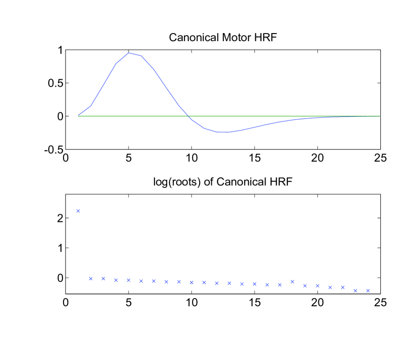
Figure 1: Canonical Motor Cortex HRF and its (log) Roots

7 Downsampling and Forwards Granger Causality

We now consider to what extent GC is preserved under downsampling.

Using the sampled notation of our discussion above, and defining $\bar{z}_{k}=\big{(}{{\bar{x}_{k}}\atop{\bar{y}_{k}}}\big{)}$, we have the following result:
Theorem VII. Forwards Causality.

(a) If $y_{t}$ dn-sgc $x_{t}$ then $\bar{y}_{k}$ dn-sgc $\bar{x}_{k}$.

(b) If $y_{t}$ dn-wgc $x_{t}$ then in general $\bar{y}_{k}$ wgc $\bar{x}_{k}$.

Remarks.

(i) Part (a) is new although technically a special case of a result of the author${}^{{}^{\prime}}$s established in a non SS framework.

(ii) We might consider taking part(b) as a formalization of long standing folklore in econometrics [6],[33] that downsampling can destroy unidirectional Granger causality. However that same folklore is flawed because it failed to recognize the possibility of (a). The folklore is further flawed because it failed to recognize the more serious reverse problem discussed below.

Proof of (a). We use the partitioned expressions in the discussion leading up to result III. We also refer to the discussion leading up to Theorem VI.

This allows us to write two decompositions. Firstly $w_{k}=w_{X,k}+w_{Y,k}$ where

$$w_{X,k}=\Sigma_{1}^{m}A^{m-i}B_{X}\epsilon_{X,km+i-1}\;\;,w_{Y,k}=\Sigma_{1}^{m}A^{m-i}B_{Y}\epsilon_{X,km+i-1}$$

From result III and the definition of dn-sgc

$$w_{X,k}\mbox{ is uncorrelated with }w_{Y,l}\mbox{ for all }k,l$$ (7.1)

The other decomposition is $\bar{\epsilon}_{k}=\big{(}{{\bar{\epsilon}_{X,k}}\atop{\bar{\epsilon}_{Y,k}}}\big{)}$ and

$$\bar{\epsilon}_{X,k}\mbox{ is uncorrelated with }\bar{\epsilon}_{Y,l}\mbox{ for all }k,l$$ (7.2)

Next we note from Theorem IV that $C_{X}(L^{-1}I-A^{m})^{-1}A^{p}B_{Y}=C_{X}\Sigma_{1}^{\infty}A^{m+r-1}B_{Y}L^{r}=0$ for all $p\geq 0$. Thus we deduce

$$C_{X}w_{Y,k}=0,\mbox{ for all }k$$ (7.3)

We can now write

$$\bar{x}_{k} = C_{X}(L^{-1}I-A^{m})^{-1}w_{k}+\bar{\epsilon}_{X,k}$$ (7.4)

$$= C_{X}(L^{-1}I-A^{m})^{-1}w_{X,k}+\bar{\epsilon}_{X,k}$$

$$\bar{y}_{k} = C_{Y}(L^{-1}I-A^{m})^{-1}w_{X,k}+C_{Y}(L^{-1}I-A^{m})^{-1}w_{Y,k}+\bar{\epsilon}_{Y,k}$$

Based on (7.4) we now introduce the ISS model for $\bar{x}_{k}$

$$\bar{x}_{k}=C_{X}(L^{-1}I-A^{m})^{-1}K_{(X)}\nu_{X,k}+\nu_{X,k}$$

where $\nu_{X,k}$ is the innovations sequence. Using this we introduce the estimator $K_{(X)}\nu_{X,k}$ of $w_{X,k}$ and the estimation error $\tilde{w}_{X,k}=w_{X,k}-K_{(X)}\nu_{X,k}$. Below we show

$$\tilde{w}_{X,k}\mbox{ is uncorrelated with }\nu_{X,l}\mbox{ for all }k,l$$ (7.5)

We thus rewrite the model for $\bar{y}_{k}$ as,

$$\bar{y}_{k} = C_{Y}(L^{-1}I-A^{m})^{-1}K_{(X)}\nu_{X,k}+\zeta_{k}$$

$$\zeta_{k} = C_{Y}(L^{-1}I-A^{m})^{-1}[w_{Y,k}+\tilde{w}_{X,k}]+\bar{\epsilon}_{Y,k}$$

Now we can construct an ISS model for $\zeta_{k}=(I+C_{Y}(L^{-1}I-A^{m})^{-1}K_{(Y)})\nu_{Y,k}$ where $\nu_{Y,k}$ is the innovations sequence. In view of (7.1,7.2,7.5) $\nu_{X,k}$ and $\nu_{Y,l}$ are uncorrelated for all $k,l$. Thus we have constructed the joint ISS model

$$\left[{{\bar{x}_{k}}\atop{\bar{y}_{k}}}\right] = \bar{H}(z)\left[{{\nu_{X,k}}\atop{\nu_{Y,k}}}\right]$$

$$\bar{H}(z) = \left[{I+C_{X}(L^{-1}I-A^{m})^{-1}K_{(X)}\atop C_{Y}(L^{-1}I-A^{m})^{-1}K_{(X)}}{0\atop I+C_{Y}(L^{-1}I-A^{m})^{-1}K_{(Y)}}\right]$$

From this we deduce that $\bar{y}_{k}$ dn-sgc $\bar{x}_{k}$ as required.

Proof of (7.5). Consider then
$E(\tilde{w}_{X,k}\nu_{X,l}^{T})=E(w_{X,k}-K_{(X)}\nu_{X,k})\nu_{X,l}^{T})=E(w_{X,k}\nu_{X,l}^{T}-K_{(X)}E(\nu_{X,k}\nu_{X,l}^{T})$. The second term vanishes for $k\neq l$. The first term vanishes for $k>l$ since $w_{X,k}$ is uncorrelated with the past and hence $\nu_{X,l}$; for $l>k$ it vanishes since $\nu_{X,l}$ is uncorrelated with the past. For $k=l$ it vanishes by the definition of $K_{(X)}$ [26].

Proof of (b). A perusal of the proof of (a) shows that we cannot construct the block lower triangular joint ISS model; in general we obtain a full block ISS model.

8 Downsampling and Reverse Granger Causality

We now come to the more serious issue of whether unidirectional Granger causality might arise from downsampling even though not present on the original timescale. To establish this we have simply to exhibit a numerical example but that is not as simple as one might hope.

8.1 Simulation Design

Designing a procedure to generate a wide class of examples of spurious causality is not as simple as one might hope. We develop such a procedure for a bivariate vector autoregression of order one; a bivariate VAR(1). On the one hand this is about the simplest example one can consider; on the other hand it is general enough to generate important behaviours.

The bivariate VAR(1) model is then,

$$\big{(}{x_{t}\atop y_{t}}\big{)}=A\big{(}{x_{t-1}\atop y_{t-1}}\big{)}+\big{(}{\epsilon_{X,t}\atop\epsilon_{Y,t}}\big{)}\;\;,A=\big{(}{\phi_{x}\atop\gamma_{y}}{\mbox{ }\gamma_{x}\atop\mbox{ }\phi_{y}}\big{)}\;\;,\Sigma=\big{(}{\sigma_{a}^{2}\atop\rho\sigma_{a}\sigma_{b}}{\mbox{ }\rho\sigma_{a}\sigma_{b}\atop\mbox{ }\sigma_{b}^{2}}\big{)}$$

where $\Sigma$ is the variance matrix of the zero mean white noise $\big{(}{\epsilon_{X,t}\atop\epsilon_{Y,t}}\big{)}$; $\rho$ is a correlation.

We note that this model can be written as an ISS model with parameters, $A,I,-A,\Sigma$. Hence all the computations desribed above are easily carried out.

But the real issue is how to select the parameters. By a straightforward scaling argument it is easy to see the we may set $\sigma_{a}=1=\sigma_{b}$ without loss of generality. Thus we need to choose only $A,\rho$.

Some reflection shows that there are two issues. Firstly we must ensure the process is stationarity i.e. for the eigenvalues $\lambda_{1},\lambda_{2}$ of $A$ we must have $|\lambda_{1}|<1,|\lambda_{2}|<1$. Secondly to design a simulation we need to choose $F_{Y\rightarrow X},F_{X\rightarrow Y}$; but these quantities depend on the parameters $A,\rho$ in a highly nonlinear way so it is not obvious how to do this. And five parameters is already too many to pursue this by trial and error.

For the first issue we have $trace(A)=\lambda_{1}+\lambda_{2}=\phi_{x}+\phi_{y}$ and $det(A)=\lambda_{1}\lambda_{2}=\phi_{x}\phi_{y}-\gamma_{x}\gamma_{y}$. Our approach is to select $\lambda_{1},\lambda_{2}$ and then find $\phi_{x},\phi_{y}$ to satisfy $\phi_{x}+\phi_{y}=\lambda_{1}+\lambda_{2},\phi_{x}\phi_{y}=\lambda_{1}\lambda_{2}+\gamma_{x}\gamma_{y}$. This requires solution of a quadratic equation. If we denote the solutions as $r_{+},r_{-}$ then we get two cases: $(\phi_{x},\phi_{y})=(r_{+},r_{-})$ and $(\phi_{y},\phi_{x})=(r_{+},r_{-})$. This leaves us to select $\gamma_{x},\gamma_{y}$.

In Appendix B we show that $F_{Y\rightarrow X}=ln\frac{\sigma_{x}^{2}}{\sigma_{a}^{2}}\geq ln(1+\xi_{x})$ where $\xi_{x}=\gamma_{x}^{2}(1-\rho^{2})$. And similarly $F_{X\rightarrow Y}\geq ln(1+\xi_{y})$ where $\xi_{y}=\gamma_{y}^{2}(1-\rho^{2})$. But we also show that $\xi_{x}=0\Rightarrow F_{Y\rightarrow X}=0$ and $\xi_{y}=0\Rightarrow F_{X\rightarrow Y}=0$. So we select $\xi_{x},\xi_{y}$ thereby setting a lower bounds to $F_{Y\rightarrow X},F_{X\rightarrow Y}$. This seems to be the best one can do and as we see below works quite well. So given $\xi_{x},\xi_{y}$ compute $\gamma_{x}=\pm\frac{\sqrt{\xi_{x}}}{\sqrt{1-\rho^{2}}}$ and $\gamma_{y}=\pm\frac{\sqrt{\xi_{y}}}{\sqrt{1-\rho^{2}}}$. This gives four cases and together with the two cases above yields eight cases.

This is not quite the end of the story since the $\gamma_{x},\gamma_{y}$ values need to be consistent with the $\phi_{x},\phi_{y}$ values. Specifically the quadratic equation to be solved for $\phi_{x},\phi_{y}$ must have real roots. Thus the discriminant must be $\geq 0$. So $(\phi_{x}+\phi_{y})^{2}-4(\phi_{x}\phi_{y})=(\lambda_{1}+\lambda_{2})^{2}-4(\lambda_{1}\lambda_{2}+\gamma_{x}\gamma_{y})=(\lambda_{1}-\lambda_{2})^{2}-4\gamma_{x}\gamma_{y}\geq 0$. There are four cases; two with real roots, two with complex roots.

If $\lambda_{1},\lambda_{2}$ are real then we require $(\lambda_{1}-\lambda_{2})^{2}\geq 4\gamma_{x}\gamma_{y}\Rightarrow(\lambda_{1}-\lambda_{2})^{2}\geq 4sign(\gamma_{x}\gamma_{y})\frac{\sqrt{\xi_{x}\xi_{y}}}{1-\rho^{2}}$. This always holds if $sign(\gamma_{x}\gamma_{y})\leq 0$. If $sign(\gamma_{x}\gamma_{y})>0$ then we have a binding constraint which restricts the sizes of $\xi_{x},\xi_{y}$.

If $\lambda_{1},\lambda_{2}$ are complex conjugates then $(\lambda_{1}-\lambda_{2})^{2}$ is negative. If $sign(\gamma_{x}\gamma_{y})\geq 0$ then the condition never holds. If $sign(\gamma_{x}\gamma_{y})<0$ then there is a binding constraint which restricts the sizes of $\xi_{x},\xi_{y}$. In particular note that if $sign(\gamma_{x}\gamma_{y})=0$ then one cannot have complex roots for $A$. We now use this design procedure to illustrate reverse causality.

8.2 Computation

We describe the steps used to generate the results below. We assume the state space model for $z_{t}=\big{(}{x_{t}\atop y_{t}}\big{)}$ comes in ISS form. Since standard state space subspace model fitting algorithms [30],[46],[1] generate ISS models this is a reasonable assumption. Otherwise we use result I to generate the corresponding ISS model.

Given a sampling multiple $m$ we first use Theorem III to generate the subsampled ISS model and hence $\Sigma_{\epsilon}^{(m)}$. To obtain the GEMs we use Theorem I to generate the marginal models for $x_{t},y_{t}$ yielding $\Omega_{X}^{(m)},\Omega_{Y}^{(m)}$. And now $F_{Y\rightarrow X}^{(m)},F_{X\rightarrow Y}^{(m)}$ are gotten from the formulae (5.8),(5.9) and the comment following Theorem Va.

8.3 Scenario Studies

We now illustrate the various results above with some bivariate simulations.

Example 1. GEMs decline gracefully.

Table 1. GEMs for various sampling intervals for
$(\lambda_{1},\lambda_{2},\xi_{x},\xi_{y},\rho)=(-.95exp(j\times.1),-.95exp(-j\times.1),1.5,.2,.2)$ $\Rightarrow A=\big{(}{-.204\atop.452}{\mbox{ }-1.24\atop\mbox{ }-1.69}\big{)}$.

m	1	2	3	4	5	6	10	20	30	40
$F_{Y\rightarrow X}$	1.3761	1.657	1.408	1.169	0.994	0.864	0.551	0.151	0.001	0.014
$F_{X\rightarrow Y}$	0.19834	0.253	0.287	0.308	0.319	0.322	0.293	0.109	0.001	0.011

Here, for the underlying process, $y$ pushes $x$ much harder than $x$ pushes $y$. This pattern is roughly preserved with slower sampling, but the relative strengths change.

Example 2. GEMs Reverse.

Table 2. GEMs for various sampling intervals for
$(\lambda_{1},\lambda_{2},\xi_{x},\xi_{y},\rho)=(.95exp(j\times.1),.95exp(-j\times.1),1.5,.2,.2)$ $\Rightarrow A=\big{(}{1.69\atop.452}{\mbox{ }-1.24\atop\mbox{ }.204}\big{)}$.

m	1	2	3	4	5	6	10	20	30	40
$F_{Y\rightarrow X}$	0.92983	0.879	0.766	0.683	0.62	0.57	0.418	0.131	0.001	0.013
$F_{X\rightarrow Y}$	1.0476	1.824	2.006	1.795	1.527	1.3	0.751	0.18	0.002	0.016

In this case the underlying processes push eachother with roughly equal strength. But subsampling yields a false picture with $x$ pushing $y$ much harder than the reverse.

Example 3. Near Equal Strength Dynamics Becomes Nearly Unidirectional.

Table 3. GEMs for various sampling intervals for
$(\lambda_{1},\lambda_{2},\xi_{x},\xi_{y},\rho)=(.995,-.7,1,.5,.7)$ $\Rightarrow A=\big{(}{1.45\atop-.84}{\mbox{ }1.18\atop\mbox{ }-1.16}\big{)}$.

m	1	2	3	4	5	6	10	20	30	40
$F_{Y\rightarrow X}$	1.487	0.051	0.245	0.057	0.111	0.052	0.038	0.019	0.012	0.009
$F_{X\rightarrow Y}$	1.685	0.167	0.638	0.258	0.467	0.294	0.289	0.212	0.159	0.125

In this case the underlying relation is one of near equal strength feedback interconnection. But almost immediately a very unequal relation appears under subsampling which soon decays to a near unidirectional relation.

Example 4. Near Unidirectional Dynamics Becomes Near Equal Strength.

Table 4. GEMs for various sampling intervals for
$(\lambda_{1},\lambda_{2},\xi_{x},\xi_{y},\rho)=(.99exp(j\times.25),.95exp(-j\times.25),.1,3,-.8)$ $\Rightarrow A=\big{(}{1.883\atop 2.236}{\mbox{ }-0.408\atop\mbox{ }0.036}\big{)}$.

m	1	2	3	4	5	6	10	20	30	40
$F_{Y\rightarrow X}$	0.023	0.284	0.381	0.428	0.451	0.457	0.309	0.454	0.407	0.168
$F_{X\rightarrow Y}$	2.937	2.384	1.617	1.243	1.019	0.859	0.372	0.532	0.453	0.178

In this case a near unidirectional dynamic relation immediately becomes one of significant but unequal strengths and then one of near equal strength.

There is nothing pathological about these examples and using the design procedure developed above it is easy to generate other similar kinds of examples. They make it emphatically clear that GC cannot be reliably discerned from subsampled data.

9 Conclusions

This paper has given a theoretical and computational analysis of the use of Granger casuality in fMRI. There were two main issues: the effect of downsampling and the effect of hemodynamic convolution. To deal with these issues a number of novel results in multivariate time series and Granger causality were developed via state space methods as follows.

1. Computations of submodels via the DARE (Theorems I,IV).

2. Reliable computation of GEMs via the DARE (Theorems Va,Vb).

3. Effect of filtering on GEMs (Theorem VI). In particular the destructive effect of the non-minimum phase property of HRFs.

4. Computation of downsampled models via the DARE.

Using these results we were able to develop, in section 8, a framework for generating downsampling induced spurious Granger causality ’on demand’ and provided a number of illustrations.

All this leads to the conclusion that that Granger causality analysis of fMRI data cannot be used to discern neuronal level driving relationships . Not only is the time-scale too slow but even with faster sampling the non-minimum phase aspect of the HRF will still compromise the method.

Future work would naturally include an extension of the Granger causality results to handle the presence of a third vector time series. And also extensions to deal with time-varying Granger causality. Non-Gaussian versions could mitigate the non-minimum phase problem to some extent but there does not seem to be any evidence for the non-Gaussianity of fMRI data. Extensions to nonlinear Granger causality are currently of great interest but need a considerable development.

10 Stabilizability, Detectability and DARE

In this section we restate and modify for our purposes some standard state space results. We rely mostly on [26][Appendices E,C].

We denote an eigenvalue of a matrix by $\lambda$ and a corresponding eigenvector by $q$. We say $\lambda$ is a stable eigenvalue if $|\lambda|<1$; otherwise $\lambda$ is an unstable eigenvalue.

10.1 Stabilizability

The pair $(A,B)$ is controllable if there exists a matrix $G$ so that $A-BG$ is stable i.e. all eigenvalues of $A-BG$ are stable. $(A,B)$ is controllable iff any of the following conditons hold,

(i) Controllability matrix: ${\mathcal{C}}=[B,AB,\cdots,A^{n-1}B]$ has rank $n$.

(ii) Rank Test: $rank[\lambda I-A,B]=n$ for all eigenvalues $\lambda$ of $A$.

(iii) PBH test: There is no left eigenvector of $A$ that is orthogonal to $B$ i.e. if $q^{T}A=\lambda q^{T}$ then $q^{T}B\neq 0$.

The pair $(A,B)$ is stabilizable if: $rank[\lambda I-A,B]=n$ for all unstable eigenvalues of $A$. Three useful tests for stabilizability are:

(i) PBH Test: $(A,B)$ is stabilizable iff there is no left eigenvector of $A$ corresponding to an unstable eigenvalue that is orthogonal to $B$ i.e. if $q^{T}A=\lambda q^{T}$ and $|\lambda|\geq 1$ then $q^{T}B\neq 0$.

(ii) $(A,B)$ is stabilizable if $(A,B)$ is controllable.

(iii) $(A,B)$ is stabilizable if $A$ is stable.

10.2 Theorem DARE

[26](Theorem E6.1, Lemma 14.2.1,section 14.7)
Under conditions, N,St,De the DARE has a unique positive semi-definite solution $P$ which is stabilizing, i.e. $A_{s}-K_{s}C$ is a stable matrix. Further if we initialize $P_{0}=0$ then $P_{t}$ is nondecreasing and $P_{t}\rightarrow P$ as $t\rightarrow\infty$.

Remarks.

(i) $A_{s}-K_{s}C$ stable means $A-KC$ is stable (see below). And this implies that $(A,K)$ is controllable (see below).

(ii) Since $V\geq R$ then $N\Rightarrow V$ is positive definite.

Proof of (i). We first note (taking limits in) [26](equation 9.5.12) $K_{s}=K-SR^{-1}$. We have then $A_{s}-K_{s}C=A-SR^{-1}C-(K-SR^{-1})C=A-KC$. So $A_{s}-K_{s}C$ is stable iff $A-KC$ is stable. But then $(A,K)$ is controllable.

10.3 Detectability

The pair $(A,C)$ is detectable if $(A^{T},C^{T})$ is stabilizable.

Remarks.

(i) If $A_{s}$ is stable (all eigenvalues have modulus $<1$) then $S,D$ automatically hold.

(ii) Condition D can be replaced with the detectability of $(A,C)$ which is the way [26] states the result. We show equivalence below (this is also noted in a footnote in [26](section 14.7).

Proof of Remark(ii). Suppose $(A_{s},C)$ is detectable but $(A,C)$ is not. Then by the PBH test there is a right eigenvector $p$ of $A$ corresponding to an unstable eigenvalue of $A$ with $Ap=\lambda p,Cp=0$. But then $A_{s}p=(A-SR^{-1}C)p=Ap=\lambda p$ while $Cp=0$ which contradicts the detectbility of $(A_{s},C)$. The reverse argument is much the same.

Proof of Result I. (a) follows from the discussion leading to theorem DARE. (b) follows from the remarks after theorem DARE.

11 GEMs for Bivariate VAR(1)

Applying formula (5.5) and reading off $H_{XX}$ etc. from the VAR(1) model yields,

$$f_{X}(\lambda) = [(1+\phi_{y}^{2}-2\phi_{y}cos(\lambda))\sigma_{a}^{2}+\gamma_{x}^{2}\sigma_{b}^{2}-2\rho\sigma_{a}\sigma_{b}(\gamma_{x}\phi_{y}-\gamma_{x}cos(\lambda))]/|D(e^{j\lambda})|^{2}$$

$$D(L) = (1-\phi_{x}L)(1-\phi_{y}L)-\gamma_{x}\gamma_{y}L^{2}$$

This can clearly be written as an ARMA(2,1) spectrum $\sigma_{x}^{2}|1-\theta_{x}e^{-j\lambda}|^{2}/|D(e^{j\lambda})|^{2}$. Equating coefficients gives

$$\gamma_{0} = \sigma_{x}^{2}(1+\theta_{x}^{2})=(1+\phi_{y}^{2})\sigma_{a}^{2}+\sigma_{b}^{2}\gamma_{x}^{2}-2\rho\sigma_{a}\sigma_{b}\gamma_{x}\phi_{y}=\sigma_{a}^{2}(1+\xi_{x}+d_{x}^{2})$$

$$\gamma_{1} = \sigma_{x}^{2}\theta_{x}=\sigma_{a}^{2}d_{x}$$

where $\xi_{x}=(1-\rho^{2})\gamma_{x}^{2}\sigma_{b}^{2}$ and $d_{x}=\phi_{y}-\rho\gamma_{x}\frac{\sigma_{b}}{\sigma_{a}}$. We thus have $\theta_{x}^{2}=\gamma_{1}^{2}/\sigma_{x}^{4}$ and using this in the first equation gives, $\gamma_{0}=\sigma_{x}^{2}+\gamma_{1}^{2}/\sigma_{x}^{2}$ or $\sigma_{x}^{4}-\sigma_{x}^{2}\gamma_{0}+\gamma_{1}^{2}=0$. This has, of course, two solutions

$$\sigma_{x}^{2} = \frac{1}{2}(\gamma_{0}\pm\sqrt{\gamma_{0}^{2}-4\gamma_{1}^{2}})$$

$$\Rightarrow\frac{\sigma_{x}^{2}}{\sigma_{a}^{2}} = \frac{1}{2}(\frac{\gamma_{0}}{\sigma_{a}^{2}}\pm\sqrt{\frac{\gamma_{0}^{2}}{\sigma_{a}^{4}}-4\frac{\gamma_{1}^{2}}{\sigma_{a}^{4}}})=\frac{1}{2}(1+\xi_{x}+d_{x}^{2}\pm\sqrt{(1+\xi_{x}+d_{x}^{2})^{2}-4d_{x}^{2}})$$

Note that if $\xi_{x}=0$ this delivers $\frac{\sigma_{x}^{2}}{\sigma_{a}^{2}}=\frac{1}{2}(1+d_{x}^{2}+\sqrt{(1-d_{x}^{2})^{2}}=1$.

We must choose the solution which ensures $|\theta_{x}|<1\equiv\frac{\gamma_{1}^{2}}{\sigma_{x}^{4}}<1\equiv\frac{\gamma_{0}}{\sigma_{x}^{4}}<2\equiv\gamma_{0}/\sigma_{a}^{2}<2\sigma_{x}^{2}/\sigma_{a}^{2}$ $\equiv 1+\xi_{x}+d_{x}^{2}<1+\xi_{x}+d_{x}^{2}\pm\sqrt{(1+\xi_{x}+d_{x}^{2})^{2}-4d_{x}^{2}}$. And so we must choose the ${}^{{}^{\prime}}$$+$${}^{{}^{\prime}}$solution. Continuing, we now claim,

$$\frac{\sigma_{x}^{2}}{\sigma_{a}^{2}}\geq\frac{1}{2}(1+\xi_{x}+d_{x}^{2}+\sqrt{(1+\xi_{x}-d_{x}^{2})^{2}}=\frac{1}{2}(1+\xi_{x}+d_{x}^{2}+1+\xi_{x}-d_{x}^{2})=1+\xi_{x}$$

This follows if, $(1+\xi_{x}+d_{x}^{2})^{2}-4d_{x}^{2}\geq(1+\xi_{x}-d_{x}^{2})^{2}\equiv(1+\xi_{x}+d_{x}^{2})^{2}-(1+\xi_{x}-d_{x}^{2})^{2}\geq 4d_{x}^{2}\equiv 2(1+\xi_{x})2d_{x}^{2}\geq 4d_{x}^{2}\equiv 1+\xi_{x}\geq 1$, which holds.

12 Spectral Factorization

Suppose $\epsilon_{t}$ is a white noise sequence with $E(\epsilon_{t})=0,var(\epsilon_{t})=\Sigma$. Let $G(L)$ be a stable causal possibly non-minimum phase filter. Then $\bar{z}_{t}=G(L)\epsilon_{t}$ has spectrum $f_{\bar{Z}}(\lambda)=G(L)VG^{T}(L^{-1})$ where $L=exp(-j\lambda)$. We can then find a unique causal, stable minimum phase spectral factorization, $f_{\bar{Z}}(\lambda)=G_{o}(L)V_{o}G_{o}^{T}(L^{-1})$. Let $V,V_{o}$ have Cholesky factorizations, $V=JJ^{T},V_{o}=J_{o}J_{o}^{T}$ and set $G_{c}(L)=G(L)J,G_{o,c}(L)=G_{o}(L)J_{o}$. Then $f_{\bar{Z}}(\lambda)=G_{c}(L)G_{c}^{T}(L^{-1})=G_{o,c}(L)G_{o,c}^{T}(L^{-1})$. Since $G_{o,c}(L)$ is minimum phase we can introduce the causal filter $E(L)=G_{o,c}^{-1}(L)G_{c}(L)\Rightarrow E(L)E^{T}(L^{-1})=I$. Such a filter is called an all pass filter [22],[19]. Now, $G_{c}(L)=G_{o,c}(L)E(L)$ or $G(L)=G_{o}(L)J_{o}E(L)J^{-1}$ i.e. a decomposition of a non-minimum phase (matrix) filter into a product of a minimum phase filter and an all pass filter. We can also write this as, $G_{o}(L)=G(L)JE^{-1}(L)J_{o}^{-1}=G(L)JE^{T}(L^{-1})J_{o}^{-1}$ showing how the non-minimum phase filter is transformed to yield a spectral factor.

References

• [1] D. Bauer. Estimating linear dynamical systems using subspace. Econometric Theory, 21:181–211, 2005.
• [2] C. Bernasconi and P. Konig. On the directionality of cortical interactions studied by structural analysis of electrophysiological recordings. Biol. Cyb., 81:199–210, 1999.
• [3] P.E. Caines. Weak and strong feedback free processes. IEEE Trans. Autom. Contr., 21:737–739, 1976.
• [4] P.E. Caines and W.W. Chan. Feedback between stationary stochastic processes. IEEE Trans. Autom. Contr., 20:498–508, 1975.
• [5] Y. Chen, S.L. Bressler, and M. Ding. Frequency domain decomposition of conditional granger causality and application to multivariate neural field potential data. Jl Neuroscience Methods’, 150:228–237, 2006.
• [6] L.J. Christiano and M. Eichenbaum. Temporal aggregation and structural inference in macroeconomics. Technical Report -, Fed Reserve Bank Minnesota, 1987.
• [7] M. Deistler, K. Peternell, and W. Scherer. Consistency and relative efficiency of subspace methods. Automatica, 31:1865–1875, 1995.
• [8] G. Deshpande, K. Sathian, and X. Hu. Effect of hemodynamic variability on granger causality analysis of fmri. Neuorimage, 52:884–896, 2010.
• [9] M. Ding, S.L. Bressler, W. Yang, and H Liang. Short-window spectral analysis of cortical event-related potentials by adaptive multivariate autoregressive modeling: data preprocessing, model validation, and variability assessment. Biol. Cyb., 83:35–45, 2000.
• [10] J.M. Dufour and E. Renault. Short and long run causality in time series; theory. Econometrica, 66:1099–1125, 1998.
• [11] J.M. Dufour and A. Taamouti. Short and long run causality measures: theory and inference. Journal of Econometrics, 154:42–58, 2010.
• [12] F. Edin. Scaling errors in measures of brain activity cause erroneous estimates of effective connectivity. NeuroImage, 49:621?630, 2010.
• [13] J. Geweke. Temporal aggregation in the multiple regression model. Econometrica, 46:643–661, 1978.
• [14] J. Geweke. The measurement of linear dependence and feedback between multiple time series. Jl. Amer. Stat. Assoc., 77:304–313, 1982.
• [15] J. Geweke. Measures conditional of linear dependence and feedback between time series. Jl. Amer. Stat. Assoc., 79:907–915, 1984.
• [16] G.H. Glover. Deconvolution of impulse response in event-related bold fmri. NeuroImage, 9:416–429, 1999.
• [17] C.W.J. Granger. Economic processes involving feedback. Information and Control, 6:28–48, 1963.
• [18] C.W.J. Granger. Investigating causal relations by econometric models and cross-spectral methods. Econometrica, 37, 1969.
• [19] M Green. All pass matrices, the positive real lemma and unit canonical correlations between future and past. Jl Multiv Anal, 24:143–154, 1988.
• [20] J. Hamilton. Time Series Analysis. Princeton Univ. Press, Princeton, New Jersey, 1994.
• [21] D.A. Handwerker, J. Gonzalez-Castillo, M. D’Esposito, and P.A. Bandettini. The continuing challenge of understanding and modeling hemodynamic variation in fmri. NeuroImage, 62:1017–1023, 2012.
• [22] E.J. Hannan and M. Deistler. Statistical theory of Linear Systems. J. Wiley, New York, 1988.
• [23] E.J. Hannan and D. Poskitt. Unit canonical correlations between future and past. Ann. Stat., 16:784–790, 1988.
• [24] R.N.A. Henson. Analysis of fmri time series: Linear time-invariant models, event-related fmri and optimal experimental design. In Human Brain Function, pages 793 – 822. Elsevier: London, 2003.
• [25] C. Hsiao. Time series modeling and causal ordering of canadian money, income and interest rates. In Time Series Analysis: Theory and Practice, North Holland, pages 671–699, 1982.
• [26] T. Kailath, A.H. Sayeed, and B. Hassibi. Linear Estimation. Prentice Hall, New York, 2000.
• [27] M.J. Kaminski and K.J. Blinowska. A new method of the description of the information flow in the brain structures. Biol. Cyb., 65:203–210, 1991.
• [28] K. Kaufmann and D.I. Stern. Evidence for human influence on climate from hemispheric temperature relations. Nature, 388:39–44, 1997.
• [29] A.M. Kshirsagar. Multivariate Analysis. Marcel Dekker, New York, 1972.
• [30] W.E. Larimore. System identification, reduced order filters and modeling via canonical variate analysis. In Proc. American Control Conference, pages 445–451. IEEE, 1983.
• [31] H. Lutkepohl. Introduction to multivariate time series analysis. Springer Verlag, Berlin, 1993.
• [32] J.R. Magnus and H. Neudecker. Matrix Differential Calculus with Applications in Statistics and Econometrics. J. Wiley, New York, 1999.
• [33] A. Marcet. Temporal aggregation of economic time series. pages 237–281, 1985.
• [34] S.M. Pandit and S. Wu. Time Series and Systems Analysis with Applications. J. Wiley, New York, 1983.
• [35] D.A. Pierce and L.D. Haugh. Causality in temporal systems characterizations and a survey. Journal of Econometrics, 5:265–293, 1977.
• [36] J. Rissannen and M. Wax. Measures of mutual and causal dependence between two time series. IEEE Trans. Inf. Thy., 33:598–601, 1987.
• [37] A. Roebroeck, E. Formisano, and R. Goebel. Mapping directed influence over the brain usng granger causality. Neuroimage, 25:230–242, 2005.
• [38] A. Roebroeck, E. Formisano, and R. Goebel. The identification of interacting networks in the brain using fmri: Model selection, causality and deconvolution. Neuroimage, 58:296–302, 2011.
• [39] G.A.F. Seber. Multivariate Observations. J. Wiley, Brisbane, 1984.
• [40] C.A. Sims. Discrete approximations to continuous time distributed lags in econometrics. Econometrica, 39:545–563, 1971.
• [41] C.A. Sims. Money, income and causality. Am. Ec. Rev., 62:540–552, 1972.
• [42] V Solo. Topics in advanced time series analysis. In Lectures in Probability and Statistics, pages 165–328. G del Pino and R Rebolledo , eds; Springer-Verlag, 1986.
• [43] L. Suna and M. Wang. Global warming and global dioxide emission: An empirical study. Jl. Environmental Management, 46(4):327–343, 1996.
• [44] L.G. Telser. Discrete samples and moving sums in stationary stochastic processes. Jl. Amer. Stat. Assoc., 62:484–499, 1967.
• [45] U. Triacca. Is granger causality analysis appropriate to investigate the relationship between atmospheric concentration of carbon dioxide and global surface air temperature? Theoretical and Applied Climatology, 81:133–135, 2005.
• [46] P. van Overschee and B. de Moor. Subspace Identification for Linear Systems. Kluwer, Dordrecht, 1996.
• [47] O. Yamashita, N. Sadato, T. Okada, and T. Ozaki. Evaluating frequency-wise directed connectivity of bold signals applying relative power contribution with the linear multivariate time-series models. Neuroimage, 25:478–490, 2005.