Microscopic Advances with Large-Scale Learning: Stochastic Optimization for Cryo-EM

Abstract

Determining the 3D structures of biological molecules is a key problem for both biology and medicine. Electron Cryomicroscopy (Cryo-EM) is a promising technique for structure estimation which relies heavily on computational methods to reconstruct 3D structures from 2D images. This paper introduces the challenging Cryo-EM density estimation problem as a novel application for stochastic optimization techniques. Structure discovery is formulated as MAP estimation in a probabilistic latent-variable model, resulting in an optimization problem to which an array of seven stochastic optimization methods are applied. The methods are tested on both real and synthetic data, with some methods recovering reasonable structures in less than one epoch from a random initialization. Complex quasi-Newton methods are found to converge more slowly than simple gradient-based methods, but all stochastic methods are found to converge to similar optima. This method represents a major improvement over existing methods as it is significantly faster and is able to converge from a random initialization.

1 Introduction

Discovering the 3D structure of molecules such as proteins and viruses is an important problem in biology and medicine. Biological macromolecules are composed of chains of simpler monomers, and the conformation or “folding” of these chains into a 3D structure determines its specific function and properties. Traditional approaches to estimating 3D structures, such as X-ray crystallography or nuclear magnetic resonance (NMR) spectroscopy, have fundamental limitations. X-ray crystallography requires a crystal of the target molecule; these are difficult to grow at best, and often impossible [24]. NMR doesn’t require a special form of the target, but is limited to relatively small molecules, preventing the study of important biological complexes [13]. Electron Cryomicroscopy (Cryo-EM) is an emerging experimental methodology for structure determination which is able to measure medium to large-sized molecules in a native state, i.e., without a need for crystallization or non-native solvents [6]. However, Cryo-EM raises challenging computational problems, one of which we attempt to address here.

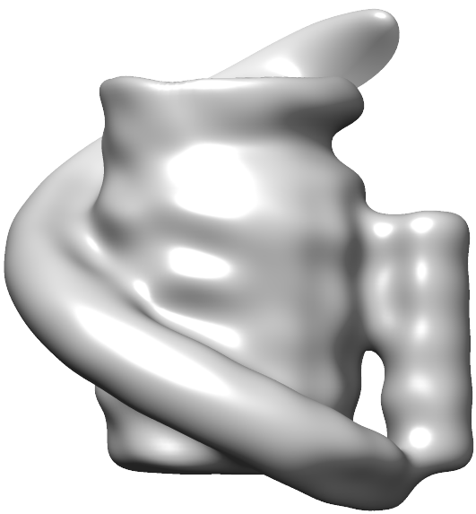
In Cryo-EM, a purified solution of target molecules is frozen in a thin film and imaged under a transmission electron microscope. The scattering of the electrons as they pass through the sample is measured, producing images in which individual molecules are visible. Each particle image is related to an orthographic, integral projection of the electron density of the target molecule, but the direction of projection is unknown. The captured image is further corrupted by destructive interference in the electron microscope imaging process and, due to the sensitive nature of biological specimens, the radiation dosage is kept to a minimum, leading to particle images with extremely low signal-to-noise ratios (SNR), typically around 0.05 [3]. The Cryo-EM imaging method, including typical particle images, is illustrated in Figure 1.

The computational task in Cryo-EM is to estimate the 3D electron density of a target molecule, given a set of particle images. This is similar to density estimation in Computed Tomography (CT), however in CT the projection direction of each image is known [11]. Together, unknown orientations and image corruption make Cryo-EM density estimation a challenging problem. Inspecting the real particle images in Figure 1 makes this clear – to the human eye the coarse dumbbell shape of the molecule is barely visible but finer details, like the presence of three stalks, are practically imperceptable.

In this paper we explore the use of stochastic optimization techniques for Cryo-EM density estimation. To do this we introduce a probabilistic latent-variable model of image formation in Cryo-EM in which we seek the maximum-a-posteriori (MAP) estimate of the electron density. We then formulate electron density estimation as a stochastic optimization problem. We show that this approach leads to significant speed gains, providing the ability to compute density estimates in just a few hours where existing approaches would take days or weeks. Further, our results show that the stochastic optimization approach is dramatically less sensitive to initialization than previous methods. While these previous approaches can be strongly biased by bad initialization [10], our method is able to quickly converge from a random initialization. We explore an array of stochastic optimization algorithms and compare their performance on a new class of objective functions which arises from the probabilistic model.

We believe that Cryo-EM is an important and challenging problem which, with a few exceptions (e.g., [19]), has seen little attention in the machine learning and computer vision communities. Our mixed results of comparing stochastic optimization methods also suggest that Cryo-EM may serve as an important benchmark problem for new stochastic optimization algorithms. While stochastic optimization algorithms have had significant success, their application has typically been limited to a small set of objective functions. With this paper we hope to spark interest in this problem at large and in Cryo-EM density estimation as a real-world benchmark for stochastic optimization methods.

2 Background and Related Work

Figure 1: A generative image formation model in Cryo-EM. The electron beam results in an orthographic integral projection of the electron density of the specimen. This projection is modulated by the Contrast Transfer Function (CTF) and corrupted with noise. The images pictured here are from a dataset of real particle images of protein ATP synthase, showcasing the low SNR typical in Cryo-EM. The zeros in the CTF make estimation particularly challenging however their location will vary as a function of experimental parameters. Particle images and density from [14].

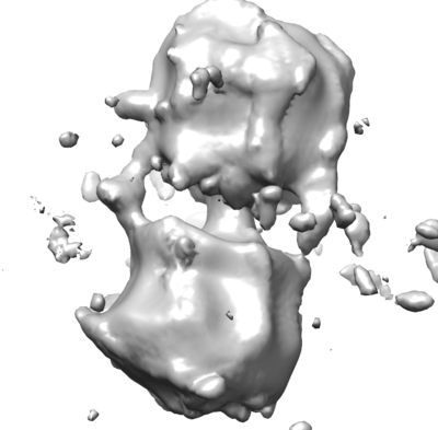
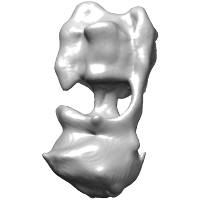
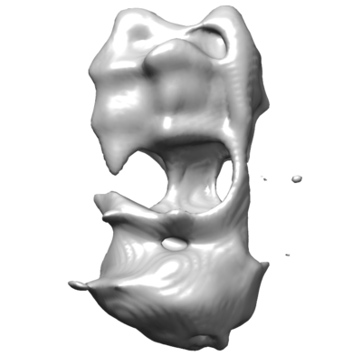
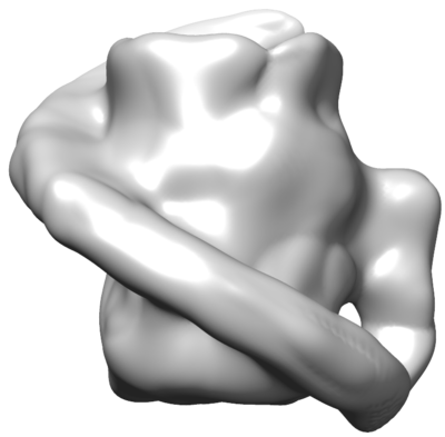
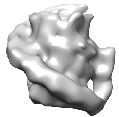
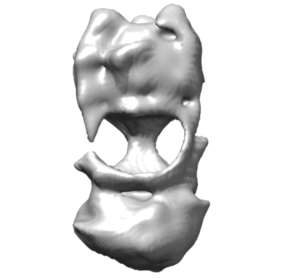
Traditional approaches to Cryo-EM density estimation, e.g., [9], aim to solve the problem by iterative refinement. An initial density estimate is projected in a large number of directions and each projection is compared with each particle image. For each particle, the projection which matches closest is considered the true orientation of the particle. Reconstruction of a new density estimate is then based on the Fourier Slice Theorem (FST) which states that the 2D Fourier transform of a projection of a density is equal to a slice through the origin of the 3D Fourier transform of that density, in a plane perpendicular to the projection direction [11]. Using the computed orientations of each particle, the new density is estimated by interpolation and averaging of the observed particle images. This approach is fundamentally limited as, even under ideal circumstances, the low SNR of particle images makes accurately identifying the single correct orientation for each particle nearly impossible resulting in errors in the estimated density. This problem is exacerbated when attempting to refine a density without prior knowledge of the shape; a poor initialization will result in estimating a structure which is either clearly wrong (see Figure 6) or, worse, appears correct but is misleading, resulting in the publication of incorrectly estimated 3D structures [10]. Finally, and crucially for the case of density estimation with many particle images, all data is used at each refinement iteration causing these methods to be slow in general.

Recently Bayesian approaches to density estimation have been proposed which avoid estimating a single orientation for individual particle images. The orientation of each particle is treated as a random variable rather than simply an unknown parameter, and all orientations are considered by marginalizing over these random variables. The resulting integral is analytically intractable but can be computed numerically. Further, the simple interpolation and averaging based off of the FST is no longer possible and some form of optimization must be performed to estimate the density. Marginalization for Cryo-EM was originally proposed for 2D image alignment by [30] and 3D reconstruction by [26]. Gradient based optimization with marginalization was originally proposed by Jaitly et al. [12] where a batch, gradient-based optimization was performed but using only a small number of low-noise images which were found by clustering and averaging individual particle images. Scheres [27] used marginalization with a batch Expectation-Maximization (EM) algorithm in the RELION package with raw particle images. In this paper we work with a similar generative model as these methods, but show that with stochastic optimization, significant progress towards a MAP estimate can be made quickly and with better robustness to initialization.

Stochastic optimization has seen significant theoretical and practical interest recently. The fundamental approach of stochastic gradient descent (SGD) remains a popular and often surprisingly effective algorithmic choice. Momentum based methods improve on SGD by using gradient information from multiple iterations, allowing for faster traversal of directions with low curvature [22, 21, 31]. Natural gradient methods have been developed based on theoretical connections to the manifold geometry of parameter space through the Fisher information matrix [2, 1] and statistical considerations of accounting for noise in gradient vectors [16, 15]. Higher-order methods have been developed which attempt to use either approximate [29, 4] or analytic Hessians [20, 15] to speed convergence by explicitly accounting for curvature. Most methods have a number of hyper-parameters and are highly sensitive to their settings; this has motivated a number of attempts to develop methods which have fewer parameters [7, 25]. Finally, when operating in the finite-data context, algorithms have been developed which can utilize the gradients of all data-points while still operating on only a limited subset at a time [17, 28] and have strong convergence results. A full review of the theoretical results is beyond the scope of this paper and we refer interested readers to [5]. In this paper we compare a number of these methods and evaluate their performance and suitability for the given task. Our results show that while some methods can find good solutions more quickly, almost all methods converge to a similarly optimal solution, and that simpler methods are typically as good or better than more complex and costly ones.

3 A Probabilistic Model of Cryo-EM

In order to formulate density estimation as an optimization problem, we turn to a probabilistic latent variable model with three parts; particle images are observed variables, their corresponding orientations are unknown latent variables, and the electron density is an unknown parameter for which we seek a MAP estimate. Each particle image is considered an orthographic, integral projection of electron density along the direction of the microscope beam. This image is corrupted by two phenomenon: the contrast transfer function (CTF) and noise.

The primary effects of the CTF, resulting from destructive interference, are modelled by a modulation in frequency space, i.e., as a linear operator on the integral projection. The Fourier spectrum of a typical CTF is shown in Figure 1. Note the phase changes and zero crossings which result in missing information in individual images. These zero crossings vary with the experimental settings of the microscope, and although each sample of target molecules can only be imaged once, different samples are imaged under different conditions to ensure that every frequency is captured. A full review of the CTF is beyond the scope of this paper and we refer interested readers to [23]. Noise arises due to the low exposure dosages necessary due to sensitive biological molecules. This noise is generally well modelled as additive IID Gaussian noise.

To formalize this, we represent an electron density as a 3D grid with density at each voxel, denoted here as $\mathcal{V}\in\mathbb{R}^{N^{3}}$ where $N$ is the side length of the cubic grid. An integral projection of this density in some orientation $\mathbf{R}\in\mathcal{SO}(3)$ can be represented as a linear transformation $\mathbf{P}_{{\mathbf{R}}}\in\mathbb{R}^{N^{2}\times N^{3}}$. We assume that each particle image $\mathcal{I}\in\mathbb{R}^{N^{2}}$ has an associated set of CTF parameters $\theta$. As discussed above, the CTF is modelled as a linear operator on the projected image, denoted here as $\mathbf{C}_{\theta}\in\mathbb{R}^{N^{2}\times N^{2}}$. Finally, the particle is subject to a 2D shift $\mathbf{t}\in\mathbb{R}^{2}$ in the image plane as it is not necessarily centered in the image which can, similarly, be represented as a linear operator denoted by $\mathbf{S}_{{\mathbf{t}}}\in\mathbb{R}^{N^{2}\times N^{2}}$. The conditional probability distribution of observing an image is thus

$$p(\mathcal{I}|\theta,\mathbf{R},\mathbf{t},\mathcal{V})=\mathcal{N}(\mathcal{I}|\mathbf{S}_{{\mathbf{t}}}\mathbf{C}_{\theta}\mathbf{P}_{{\mathbf{R}}}\mathcal{V},\sigma^{2}\mathbf{I})$$ (1)

where $\sigma$ is the standard deviation of the noise and $\mathcal{N}(\mu,\Sigma)$ is the multivariate normal distribution with mean vector $\mu$ and covariance matrix $\Sigma$. In practice due to computational considerations Equation 1 is evaluated in Fourier space, making use of the Fourier Slice Theorem and Parseval’s Theorem to obtain

$$p(\tilde{\mathcal{I}}|\theta,\mathbf{R},\mathbf{t},\tilde{\mathcal{V}})=\mathcal{N}(\tilde{\mathcal{I}}|\tilde{\mathbf{S}}_{{\mathbf{t}}}\tilde{\mathbf{C}}_{\theta}\tilde{\mathbf{P}}_{{\mathbf{R}}}\tilde{\mathcal{V}},\sigma^{2}\mathbf{I})$$ (2)

where $\tilde{\mathcal{I}}$ is the Fourier transform of the image, $\tilde{\mathbf{S}}_{{\mathbf{t}}}$ is the shift operator in Fourier space (a phase change), $\tilde{\mathbf{C}}_{\theta}$ is the CTF modulation in Fourier space (a diagonal operator), $\tilde{\mathbf{P}}_{{\mathbf{R}}}$ is a sinc interpolation operator which extracts a plane through the origin defined by the projection orientation $\mathbf{R}$ and $\tilde{\mathcal{V}}$ is the 3D Fourier transform of $\mathcal{V}$. To further speed computation of the likelihood, and because of the level of noise and the attenuation of high frequencies by the CTF, Equation 2 is only evaluated using Fourier coefficients up to a specified maximum frequency.

Figure 2: The synthetic density (left) and simulated images (right) generated by choosing orientations uniformly at random, applying CTFs selected from a real dataset and adding noise.

This image formation model provides the conditional probability of observing an image $\tilde{\mathcal{I}}$ from a given orientation, shift and density. The orientation and shift, however, are unknown. To cope with this, we marginalize over these latent variables [12, 27] and, assuming they are independent of each other and the density $\mathcal{V}$, get

$$p(\tilde{\mathcal{I}}|\theta,\tilde{\mathcal{V}})=\int_{\mathbb{R}^{2}}\int_{\mathcal{SO}(3)}p(\tilde{\mathcal{I}}|\theta,\mathbf{R},\mathbf{t},\tilde{\mathcal{V}})p(\mathbf{R})p(\mathbf{t})d\mathbf{R}d\mathbf{t}$$ (3)

where $p(\mathbf{R})$ is the uniform distribution over $\mathcal{SO}(3)$ and we use a normal distribution truncated based on the size of the particle images for the shift distribution $p(\mathbf{t})$. This double integral is not analytically tractable and so we resort to numerical quadrature. We use Lebedev quadrature over directions of projection in $\mathcal{S}^{2}$ combined with uniform quadrature over the interval $[0,2\pi)$ to account for in-plane rotation [18, 8] and uniform quadrature over the truncated region of $\mathbb{R}^{2}$ to account for shifts. Using numerical quadrature, the conditional probability of an image is

$$p(\tilde{\mathcal{I}}|\theta,\tilde{\mathcal{V}})\approx\sum_{j=1}^{M}w_{j}p(\tilde{\mathcal{I}}|\theta,\mathbf{R}_{j},\mathbf{t}_{j},\tilde{\mathcal{V}})$$ (4)

where $\{(\mathbf{R}_{j},\mathbf{t}_{j},w_{j})\}_{j=1}^{M}$ are the weighted quadrature points. The accuracy of the quadrature scheme, and consequently the value of $M$, is set automatically based on the specified maximum frequency considered.

Given a set of $K$ images with CTF parameters $\mathfrak{D}=\{(\mathcal{I}_{i},\theta_{i})\}_{i=1}^{K}$ and assuming conditional independence of the images, the posterior is

$$p(\mathcal{V}|\mathfrak{D})\propto p(\mathcal{V})\prod_{i=1}^{K}p(\tilde{\mathcal{I}}_{i}|\theta_{i},\tilde{\mathcal{V}})$$ (5)

where $p(\mathcal{V})$ is a prior. We use a combination of an exponential distribution for positive density values to encourage sparsity and a generalized normal distribution to softly penalize negative density values. Specifically, $p(\mathcal{V})=\prod_{i=1}^{N^{3}}p(\mathcal{V}_{i})$ where $\mathcal{V}_{i}$ is the value of the $i$th voxel, $p(\mathcal{V}_{i})\propto e^{-\lambda_{+}\mathcal{V}_{i}}$ if $\mathcal{V}_{i}\geq 0$, and $p(\mathcal{V}_{i})\propto e^{-\lambda_{-}|\mathcal{V}_{i}|^{3}}$ if $\mathcal{V}_{i}<0$. Many other choices of prior are possible and is a promising direction for future research.

Estimating the electron density then corresponds to finding $\mathcal{V}$ which maximizes Equation 5. Optimizing this directly is costly due to the marginalization in Equation 4. When selecting a maximum frequency cut-off of only 16% of the Nyquist limit, this corresponds to approximately $95,000$ quadrature points for the datasets shown here. Combined with a dataset size of around $46,000$ particle images, a full evaluation of the posterior and its gradient takes over a day of computation time on a modern CPU. Instead, we formulate this as a stochastic optimization problem. Taking the log and dropping constant factors the optimization problem becomes

$$\arg\min_{\mathcal{V}}-\sum_{i=1}^{K}\left(\log p(\tilde{\mathcal{I}}_{i}|\theta_{i},\tilde{\mathcal{V}})+K^{-1}\log p(\mathcal{V})\right)$$ (6)

which is the standard form for a stochastic optimization problem.

Figure 3: The negative log likelihood of the test data versus the number of gradient evaluations for the synthetic (left) and Thermus (right) datasets with a zoomed in view of the final iterations.

3.1 Discussion

Before presenting our results we discuss some general observations about this objective function. First, in the neighbourhood of a solution $\mathcal{V}^{*}$ which explains each particle image well enough that only a single term (corresponding to a single orientation and shift) in Equation 4 is significant, Equation 6 becomes the sum of the log prior term and $K$ quadratic terms in $\mathcal{V}$. Thus, near $\mathcal{V}^{*}$, the objective is roughly an L1 regularized linear least squares problem and thus is approximately convex.

In general, the objective function has the algebraic form of a mixture model posterior due to the sum in Equation 4. Each orientation is analogous to a mixture component, with parameters corresponding to the respective slice of $\tilde{\mathcal{V}}$. One might suspect the typical pathologies of mixture models to manifest such as overfitting when some components (i.e., orientations) are assigned only a small number of data points. However unlike a mixture model, in this problem the parameters of each component are interrelated, as each is a linear combination of elements of $\tilde{\mathcal{V}}$. In particular, low frequency coefficients are shared with many mixture components, while progressively higher frequencies are shared by fewer and fewer.

Taken together, these observations suggest that, while the objective function in Equation 6 is not convex, it should be well behaved so long as the low-frequency Fourier coefficients are approximately correct. This observation can also be seen as further motivation for only considering Fourier coefficients below a threshold, as we expect the restricted problem to be better behaved. In practice, when higher resolution structures are sought a good strategy would be to introduce high-frequency Fourier coefficients gradually.

4 Experiments

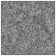
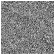
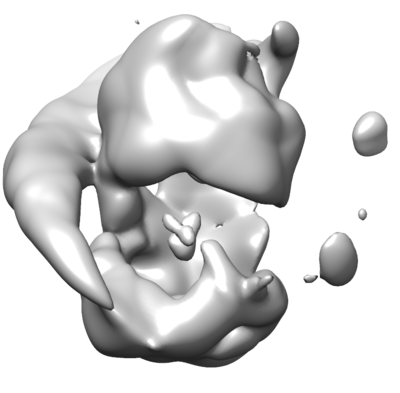
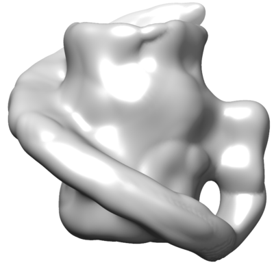
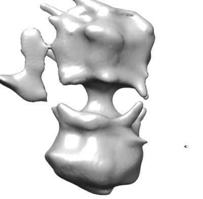
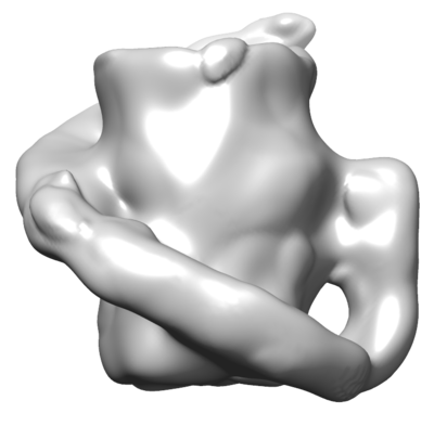
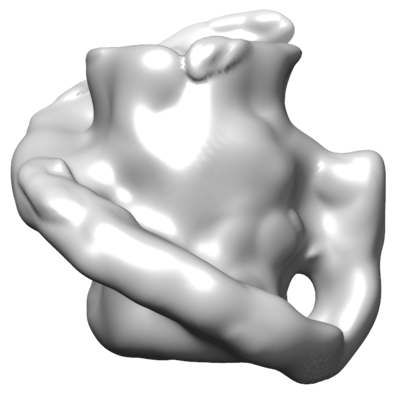
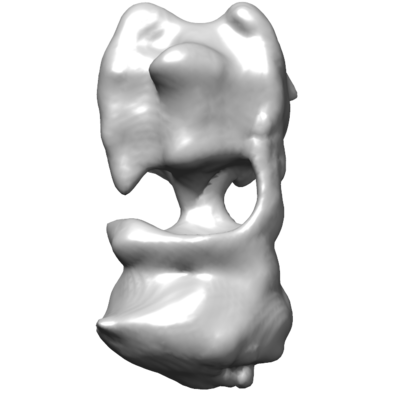
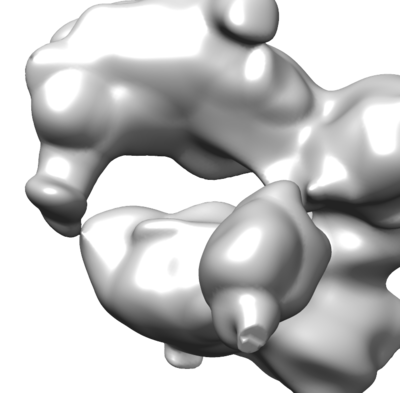
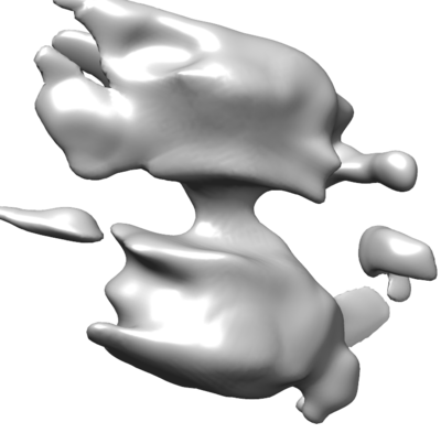
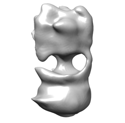
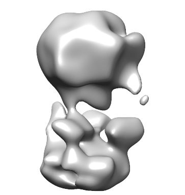
To explore the potential of different optimization methods we acquired two datasets, one synthetic and one real. The real dataset is of ATP synthase from the Thermus thermophilus bacteria, which is a large transmembrane molecule which provides energy to cells. The dataset, consisting of $46,105$ particle images and CTF parameters, was provided by Lau and Rubinstein [14]. The high resolution structure from [14] and some sample images are shown in Figure 1. As a specimen for Cryo-EM this dataset is known to be challenging as there is no particle symmetry and the contrast is low. The second dataset was synthetically created using a simple, hand crafted electron density. Using that density, $50,000$ particle images were generated by uniformly sampling random orientations and assuming zero in-plane translation. CTFs were simulated with parameters randomly selected from the Thermus dataset and noise was added to have a comparable SNR. The synthetic density and some simulated images are shown in Figure 2.

	Synthetic (50K Images)			Thermus (46K Images)
	$5$K	$50$K	Final	$5$K	$50$K	Final
SGD
AdaGrad
CM
NAG
TONGA
oLBFGS
HF

Figure 4: Estimated structures after $5$K, $50$K and all gradient evaluations (10 epochs) on two datasets, using seven different stochastic optimization methods.

Optimization Methods.

Optimization was performed on these datasets with seven different stochastic optimization algorithms. Specifically, we used traditional stochastic gradient descent (SGD), SGD with classical momentum (CM) [22], SGD with Nesterovs Accelerated Gradient (NAG) [21, 31], AdaGrad [7], TONGA [16], Online LBFGS [29] and Hessian-Free optimization (HF) [20]. Particle images for both datasets are $128\times 128$ pixels and their values were rescaled by the standard deviation of noise so that $\sigma=1$. Prior parameters were set to $\lambda_{+}=10^{-4}$ and $\lambda_{-}=10^{-4}$ for the synthetic dataset and $\lambda_{+}=3\times 10^{-2}$ and $\lambda_{-}=10^{-4}$ for the Thermus dataset. Fourier coefficients were considered out to a radius of 10% of the Nyquist limit for the synthetic dataset and 16% for Thermus. A minibatch size of $100$ was used for all methods except HF. For HF, 5 conjugate gradient iterations were used with a minibatch size of $300$ and a damping parameter which was tuned by hand. The larger minibatch size was chosen as a trade-off; smaller minibatches required strong damping which resulted in small step sizes and slower convergence.

The base learning rate was tuned by hand for each method by examining performance on a subset of the training examples. For all methods except AdaGrad and HF, the learning rate is annealed according to $\eta_{t}=\eta_{0}(1+\lambda t)^{-0.75}$ where $\lambda=10^{-2}$, $t$ is the iteration number and $\eta_{0}$ is a base learning rate. The momentum parameters for CM and NAG were set to $\min\{0.9,1-2^{-1-\log_{2}(\lfloor\frac{t}{100}\rfloor+1)}\}$ [31]. For TONGA the covariance matrix was approximated with a rank $20$ approximation after every $20$ iterations and the regularization parameter was tuned along with the learning rate.

Figure 5: The random initialization used in all experiments, generated by summing random spheres.

Online LBFGS used $m=30$ update vectors to approximate the inverse Hessian. All methods were run for $10$ epochs except for HF and Online LBFGS which were run for fewer iterations to account for the increased number of gradient evaluations needed for these methods.

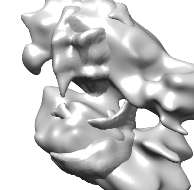
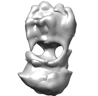
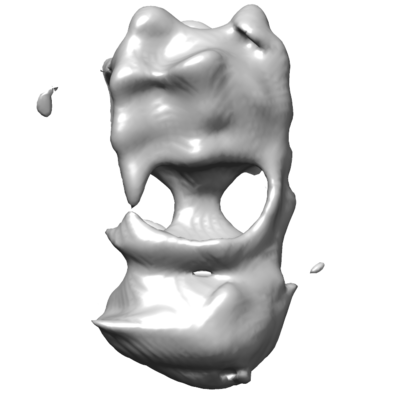
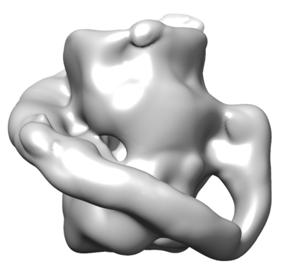
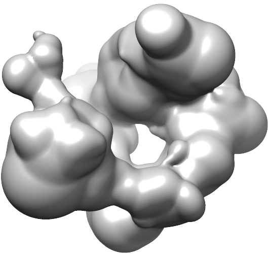
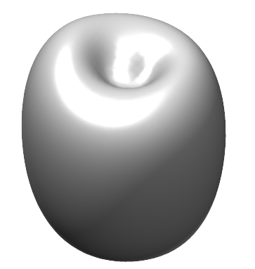
For both datasets $100$ particle images were randomly held out as a test set and the negative log likelihood on the test set used to measure performance. The remaining images were randomly shuffled with each method seeing the images in the same order. In each case, optimization was initialized with the same randomly constructed density shown in Figure 5.

Stochastic Optimization Results.

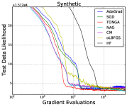
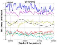
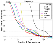
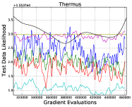
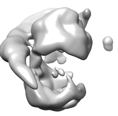
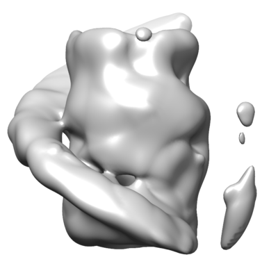
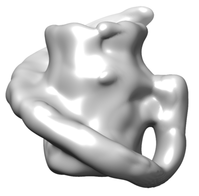
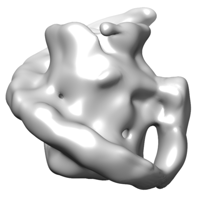
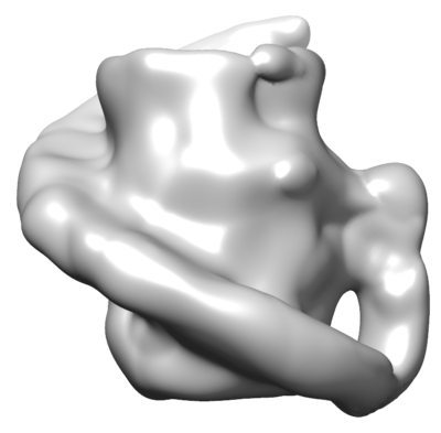
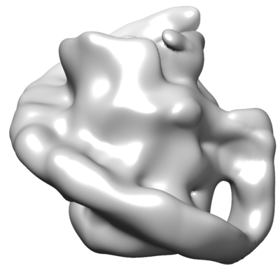
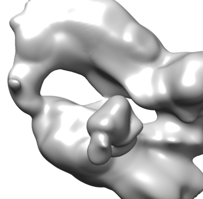
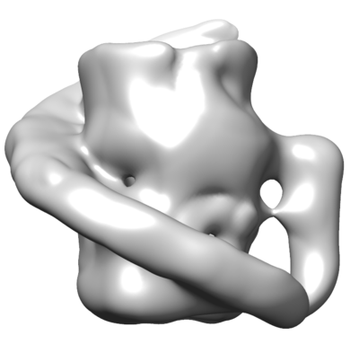
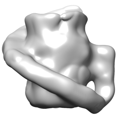
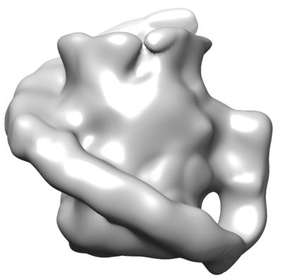
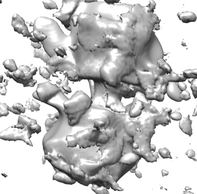
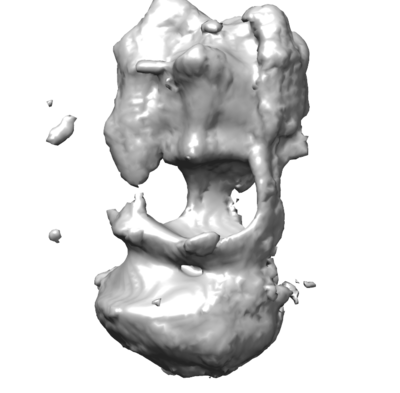
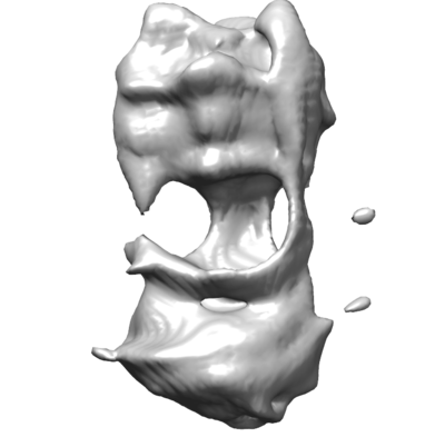
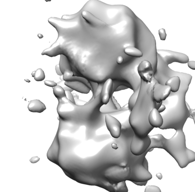
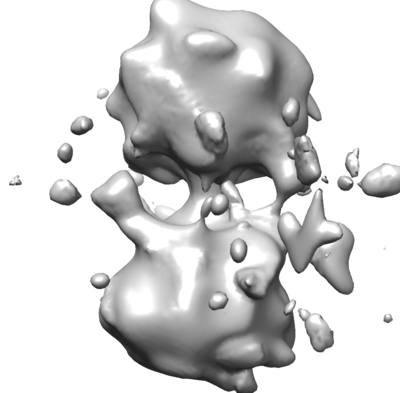
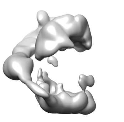
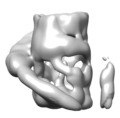
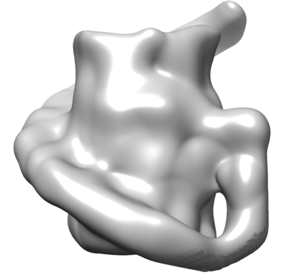
Results of the optimizations are plotted in Figure 3 versus the number of gradients of individual particle images. This was used to account for the additional gradient evaluations required by Online LBFGS and the different minibatch sizes and Hessian-vector products (implemented with a directional finite difference) required by HF. We show the estimated densities throughout optimization in Figure 4. Note that all algorithms were able to find reasonable solutions eventually, with the final data likelihood of all methods being within two log units of each other. In terms of speed, an epoch (or equivalent) took approximately one hour using 32 threads on a quad, eight core 2.9GHz Intel Xeon CPU. Looking at the plots in Figure 3 we can make some observations about the efficacy of individual methods.

First, note that behaviour is different between the synthetic and real datasets. We suspect that outliers in the Thermus dataset are to blame for part of this difference. While the image formation model described in the previous section is a good approximation which has been well established in the Cryo-EM literature, it is not perfect. Further, the particle images were manually selected from large micrographs and mistakes can be made due the high signal-to-noise ratio as well as simple human error. An additional difference between the two datasets is the shape of the structure itself. The strong cylindrical shape of the synthetic structure causes the objective function to have directions of low curvature at early iterations resulting from this symmetry. Methods which are able to efficiently traverse through these regions are likely to do better. Note that structures like this are not uncommon in nature, as many molecules of interest, in particular viruses, have strong symmetries.

With this in mind, we note that TONGA and the momentum methods (CM and NAG) do well on the synthetic dataset as might have been predicted while AdaGrad and SGD clearly slow down around $10^{4}$ as they traverse this low-curvature area. Online LBFGS does not appear to plateau in the same way as SGD and AdaGrad, but the added cost of the extra gradient evaluations needed to compute the update vectors for LBFGS are not outweighed by the faster progress it is able to make at each iteration. In comparison, on the Thermus dataset this low curvature area does not appear to be present due to the asymmetry of the particle, resulting in a similar qualitative behaviour of the methods. That said, SGD, AdaGrad and TONGA generally converge faster than Online LBFGS or the momentum methods. For both datasets, however, the story with Hessian-Free optimization is consistent: the added cost of the CG iterations and larger minibatches may allow faster progress in a given iteration, but that progress does not outweigh the additional computational cost.

Comparison to State-of-the-Art.

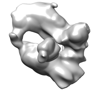
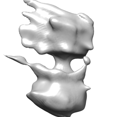
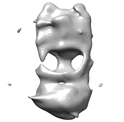
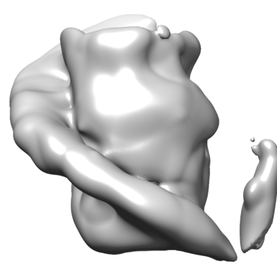
To compare this method to existing methods for structure determination, we selected two approaches. The first is a standard iterative projection matching scheme where images are matched to an initial density through a global cross-correlation search. The density is then reconstructed based on these orientations and this process is iterated. The second is the RELION package described in [27] which uses a similar marginalized model as our method but with a batch EM algorithm to perform optimization. We used publicly available code for both of these approaches and initialized using the density shown in Figure 5.

We ran each method for five iterations, roughly equivalent computationally to five epochs or $250,000$ gradient evaluations for our method. The results after five iterations of these methods are shown in Figure 6. In both cases the approaches failed to converge in the time allotted, particularly when compared with the structures estimated by the proposed approach with approximately a fifth of computation, i.e., the $50,000$ columns in Figure 4.

Projection Matching	RELION	Proposed Approach
5 Epochs	5 Epochs	1 Epoch

Figure 6: Baseline comparisons to two existing standard methods. Iterative projection matching and reconstruction (left) and RELION [27] (middle) after 5 batch iterations. The proposed method (right) with SGD after just one epoch.

5 Conclusions

This paper has introduced and motivated the challenging problem of density estimation for Cryo-EM, formulated it using a probabilistic image formation model and cast the resulting MAP estimation problem as a stochastic optimization. We have implemented an array of seven stochastic optimization methods ranging from simple SGD through momentum methods to more complex quasi-Newton methods and compared their behaviour and performance on the CryoEM problem with both real and synthetic data. A comparison of our proposed stochastic optimization approach with current methods demonstrates that stochastic optimization yields significant speedups and robustness to initialization. The proposed approach converges to reasonable structures in as little as one epoch from a random initialization while, in comparison, existing methods make slow progress even after many epochs, or become trapped in local minima. Among the stochastic optimization methods tested, we find that all are effective at finding a good solution, though some typically converge faster than others. Notably we find that methods which require significant additional computation per iteration like Online LBFGS [29] or Hessian-free optimization [20] do not perform better than simply taking more iterations of other methods on this problem.

We believe that the problem of density estimation for CryoEM is an important problem and an interesting challenge for stochastic optimization algorithms in general. In particular, this work highlights one of the major limitations of most existing methods: their reliance on manual tuning. All methods had parameters which required some amount of manual tuning and every dataset would potentially require those parameters to be re-adjusted. While efforts were made to standardize the datasets, some amount of retuning is generally necessary for each new dataset. More research is needed to develop methods which are able to automatically adapt to different objective functions and we note that there are several methods which show significant promise along these lines [7, 17, 28, 25].

References

- Amari et al. [2000] S.-I. Amari, H. Park, and K. Fukumizu. Adaptive method of realizing natural gradient learning for multilayer perceptrons. Neural Computation, 12(6):1399–1409, 2000.
- Amari [1998] S.I. Amari. Natural gradient works efficiently in learning. Neural Computation, 10(2):251–276, 1998.
- Baxter et al. [2009] William T Baxter, Robert A Grassucci, Haixiao Gao, and Joachim Frank. Determination of signal-to-noise ratios and spectral snrs in cryo-em low-dose imaging of molecules. J Struct Biol, 166(2):126–32, May 2009.
- Bordes et al. [2009] Antoine Bordes, Léon Bottou, and Patrick Gallinari. Sgd-qn: Careful quasi-newton stochastic gradient descent. J. Mach. Learn. Res., 10:1737–1754, December 2009.
- Bottou and Bousquet [2011] Léon Bottou and Olivier Bousquet. The tradeoffs of large scale learning. In Optimization for Machine Learning, pages 351–368. MIT Press, 2011.
- Chiu [1993] W Chiu. What does electron cryomicroscopy provide that x-ray crystallography and nmr spectroscopy cannot? Annual Review of Biophysics and Biomolecular Structure, 22(1):233–255, 1993.
- Duchi et al. [2011] John Duchi, Elad Hazan, and Yoram Singer. Adaptive subgradient methods for online learning and stochastic optimization. J. Mach. Learn. Res., 12:2121–2159, July 2011.
- Gräf and Potts [2009] Manuel Gräf and Daniel Potts. Sampling sets and quadrature formulae on the rotation group. Numerical Functional Analysis and Optimization, 30(7-8):665–688, 2009.
- Grigorieff [2007] N. Grigorieff. Frealign: high-resolution refinement of single particle structures. J Struct Biol, 157(1):117–125, Jan 2007.
- Henderson et al. [2012] R Henderson, A Sali, M L Baker, B Carragher, B Devkota, K H Downing, E H Egelman, Z Feng, J Frank, N Grigorieff, W Jiang, S J Ludtke, O Medalia, P A Penczek, P B Rosenthal, M G Rossmann, M F Schmid, G F Schröder, A C Steven, D L Stokes, J D Westbrook, W Wriggers, H Yang, J Young, H M Berman, W Chiu, G J Kleywegt, and C L Lawson. Outcome of the first electron microscopy validation task force meeting. Structure, 20(2):205 – 214, 2012.
- Hsieh [2003] Jiang Hsieh. Computed Tomography: Principles, Design, Artifacts, and Recent Advances. SPIE, 2003.
- Jaitly et al. [2010] Navdeep Jaitly, Marcus A. Brubaker, John Rubinstein, and Ryan H. Lilien. A Bayesian Method for 3-D Macromolecular Structure Inference using Class Average Images from Single Particle Electron Microscopy. Bioinformatics, 26:2406–2415, 2010.
- Keeler [2010] James Keeler. Understanding NMR Spectroscopy. Wiley, 2010.
- Lau and Rubinstein [2012] Wilson C. Y. Lau and John L. Rubinstein. Subnanometre-resolution structure of the intact Thermus thermophilus H+-driven ATP synthase. Nature, 481:214–218, 2012.
- Le Roux and Fitzgibbon [2010] Nicolas Le Roux and Andrew Fitzgibbon. A fast natural Newton method. In ICML, 2010.
- Le Roux et al. [2008] Nicolas Le Roux, Pierre-Antoine Manzagol, and Yoshua Bengio. Topmoumoute online natural gradient algorithm. In NIPS, pages 849–856, 2008.
- Le Roux et al. [2012] Nicolas Le Roux, Mark Schmidt, and Francis Bach. A stochastic gradient method with an exponential convergence rate for strongly convex optimization with finite training sets. In NIPS, 2012.
- Lebedev and Laikov [1999] V. J. Lebedev and D. N. Laikov. A quadrature formula for the sphere of the 131st algebraic order of accuracy. Doklady Mathematics, 59(3):477 – 481, 1999.
- Mallick et al. [2006] Satya Mallick, Sameer Agarwal, David Kriegman, Serge Belongie, Bridget Carragher, and Clint Potter. Structure and view estimation for tomographic reconstruction: A bayesian approach. In CVPR, 2006.
- Martens [2010] James Martens. Deep learning via hessian-free optimization. In ICML, 2010.
- Nesterov [1983] Yurii Nesterov. A method of solving a convex programming problem with convergence rate o (1/k2). Soviet Mathematics Doklady, 27(2):372–376, 1983.
- Polyak [1964] B.T. Polyak. Some methods of speeding up the convergence of iteration methods. USSR Computational Mathematics and Mathematical Physics, 4(5):1–17, 1964.
- Reimer and Kohl [2008] Ludwig Reimer and Helmut Kohl. Transmission Electron Microscopy: Physics of Image Formation. Springer, 2008.
- Rupp [2009] B Rupp. (2009). Biomolecular Crystallography: Principles, Practice and Application to Structural Biology. Garland Science, 2009.
- Schaul et al. [2013] Tom Schaul, Sixin Zhang, and Yann LeCun. No More Pesky Learning Rates. In ICML, 2013.
- Scheres et al. [2007] Sjors H W Scheres, Haixiao Gao, Mikel Valle, Gabor T Herman, Paul P B Eggermont, Joachim Frank, and Jose-Maria Carazo. Disentangling conformational states of macromolecules in 3d-em through likelihood optimization. Nature Methods, 4:27–29, 2007.
- Scheres [2012] Sjors H.W. Scheres. RELION: Implementation of a Bayesian approach to cryo-EM structure determination . Journal of Structural Biology, 180(3):519 – 530, 2012.
- Schmidt et al. [2013] Mark Schmidt, Nicolas Le Roux, and Francis Bach. Minimizing finite sums with the stochastic average gradient. Technical report, 2013.
- Schraudolph et al. [2007] Nicol N. Schraudolph, Jin Yu, and Simon Günter. A stochastic quasi-newton method for online convex optimization. JMLR, 2:436–443, 2007.
- Sigworth [1998] F.J. Sigworth. A maximum-likelihood approach to single-particle image refinement. Journal of Structural Biology, 122(3):328 – 339, 1998.
- Sutskever et al. [2013] Ilya Sutskever, James Martens, George Dahl, and Geoffrey Hinton. On the importance of initialization and momentum in deep learning. In ICML, 2013.