Fast, approximate kinetics of RNA folding

Abstract

In this paper, we introduce the software suite, Hermes, which provides fast, novel algorithms for RNA secondary structure kinetics. Using the fast Fourier transform to efficiently compute the Boltzmann probability that a secondary structure $S$ of a given RNA sequence has base pair distance $x$ [resp. $y$] from reference structure $A$ [resp. $B$], Hermes computes the exact kinetics of folding from $A$ to $B$ in this coarse-grained model. In particular, Hermes computes the mean first passage time from the transition probability matrix by using matrix inversion, and also computes the equilibrium time from the rate matrix by using spectral decomposition. Due to the model granularity and the speed of Hermes, it is capable of determining secondary structure refolding kinetics for large RNA sequences, beyond the range of other methods. Comparative benchmarking of Hermes with other methods indicates that Hermes provides refolding kinetics of accuracy suitable for use in computational design of RNA, an important area of synthetic biology. Source code and documentation for Hermes are available at http://bioinformatics.bc.edu/clotelab/Hermes/.

1 Introduction

Remarkable results in RNA synthetic biology have recently been obtained by various groups. In [25], small conditional RNAs have been engineered to silence a gene Y by using the RNA interference machinery, only if a gene X is transcribed. In [43] a novel theophylline riboswitch has been computationally designed to transcriptionally regulate a gene in E. coli, and in [7] a purely computational approach was used to design functionally active hammerhead ribozymes. Computational design of synthetic RNA molecules invariably uses some form of thermodynamics-based algorithm; indeed, NUPACK-Design [49] was used to design small conditional RNAs [25], Vienna RNA Package [23] was used in the design of the synthetic theophylline riboswitch, and the RNAiFold inverse folding software [19, 18] was used to design the synthetic hammerhead ribozymes. The next step in the computational design of synthetic RNA molecules is to control the kinetics of folding – such control could be important in engineering conformational switches. Kinetics is already used as a design feature for synthetic design in proteins [4, 8].

In this paper, we introduce a new software suite, called Hermes, which efficiently computes RNA secondary structure folding kinetics by using a coarse-grained method to model RNA transitions that add or remove a single base pair. Since our motivation in developing Hermes is to provide a new tool to aid in engineering synthetic RNA molecules with desired kinetic properties, Hermes does not model co-transcriptional folding, but only the refolding of RNA sequences.

There is a long history of both experimental and computational work on RNA folding pathways and kinetics, so much so, that a review of previous work is beyond the scope of this paper. Here we cite only the most relevant related work on RNA secondary structure kinetics. Experimental approaches to determine the kinetics of RNA folding include temperature jump experiments [28], using fluorophores [24], using mechanical tension at the single molecule level [42], etc. and will not be further discussed. In this paper we focus exclusively on computational approaches to folding kinetics, where stepwise transitions between secondary structures involve the addition or removal of a single base pair, as first considered in [12]. Nevertheless, it should be noted that there are a number of methods that concern the addition or removal of an entire helical region, e.g. [26, 50].

Most computational approaches involve either (1) algorithms to determine optimal or near-optimal folding pathways, (2) explicit solutions of the master equation, (3) repeated simulations to fold an initially empty secondary structure to the target minimum free energy (MFE) structure. Examples of methods to determine optimal or near-optimal folding pathways include the greedy approach of Morgan and Higgs [34], the exact, optimal, exponential time program barriers [12], the program Findpath [11], which uses bounded look-ahead breadth-first search, a genetic algorithm [37], the program RNAtabupath that uses local search to determine near-optimal folding pathways, etc. The program barriers [12] is the only current method guaranteed to produce optimal folding pathways. Since it has been shown that the problem of determining optimal folding pathways is NP-complete [40], it is now understandable why barriers can take exponential time to converge, depending on the RNA sequence. For this reason, near-optimal solutions provided by heuristic methods, such as RNAtabupath, are very useful.

Methods that employ the master equation include Treekin [45], which uses the programs RNAsubopt [47] and barriers [12] to determine macrostates, defined as basins of attraction near a locally optimal structure. The resulting coarse-grained Markov chain is then sufficiently small to allow explicit solution of the master equation. In [38], a moderate number of RNA structures were sampled according to different strategies, from which a robotic motion planning graph was defined to connect each sampled structure to its $k$ nearest sampled neighbors. Again, the resulting coarse-grained Markov chain is sufficiently small for an explicit solution of the master equation to be given.

We now come to simulation approaches to estimate RNA folding kinetics. The program Kinfold [9, 10] is an implementation of Gillespie’s algorithm [22], directly related to the master equation, hence is considered by many to be the gold standard for RNA kinetics. A recent extension of the Kinfold algorithm was reported in [3]. Kinefold [48] uses stochastic simulations of the nucleation and dissociation of helical regions to predict secondary structure and folding pathways. In contrast to the previously mentioned methods, both RNAKinetics [6] and Kinwalker [21] model co-transcriptional folding, known to be necessary when simulating in vivo folding of long RNA molecules [27]. As well, Kinefold can simulate both refolding and co-transcriptional folding pathways. Finally, unlike all the previous simulation results, which depend on thermodynamic free energy parameters [41], the program Oxfold [1] performs kinetic folding of RNA using stochastic context-free grammars and evolutionary information.

In contrast to the previous methods, Hermes computes the mean first passage time (MFPT) and equilibrium time for a coarse-grained Markov chain consisting of the ensemble of all secondary structures having base pair distance $x$ [resp. $y$] from reference structures $A$ [resp. $B$] of a given RNA sequence. Mean first passage time (MFPT) is computed exactly by matrix inversion, and equilibrium time is computed using spectral decomposition of the rate matrix for the coarse-grained master equation. Hermes is written in C/C++, and makes calls to the Fast Fourier Transform implementation FFTW [17] http://www.fftw.org/, the Gnu Scientific Library (GSL) http://www.gnu.org/software/gsl/, and the free energy functions from Vienna RNA Package [29]. The plan of the paper is as follows.

Section 2 gives background definitions and results concerning Markov chains, Markov processes, mean first passage time (MFPT), and equilibrium time (ET). This section can be skipped for those readers who are familiar with kinetics. For sufficiently small RNA sequences, MFPT and ET are computed by Hermes using the methods described in this section, and so can provide a gold and platinum standard against which other kinetics methods can be compared. Other methods include simulation methods such as the Monte Carlo algorithm and the Gillespie algorithm, and computations of MFPT and ET for coarse-grained Markov chains that partition secondary structures into disjoint macrostates. Section 3 presents an overview of the software suite Hermes, which consists of three C/C++ software packages (FFTbor2D, RNAmfpt, RNAeq) and two C-driver programs (FFTmfpt, FFTeq). Section 4 presents the benchmarking results, which compare Hermes with existent RNA kinetics software by using a collection of 1000 random 20-mers, for which accurate mean first passage times and equilibrium times can be exactly computed. Our objective here is to show that kinetics obtained by using coarse-grained methods from Hermes correlate well with the gold and platinum standards, yet are sufficiently fast to be used in synthetic biology applications. Slower methods having finer granularity may subsequently of great use in detailed kinetics studies of one or a small number of sequences. Section 5 summarizes the contribution of Hermes, and the Appendix presents detailed descriptions of all the kinetics methods and parameters used in the benchmarking results reported in Section 4.

2 Preliminaries

To better understand the underlying algorithms behind the software, we describe two traditional approaches in kinetics.

2.1 Markov chains and mean first passage time

Consider a physical process, which when monitored over time, yields the stochastic sequence $q_{0},q_{1},q_{2},\ldots$ of discrete, observed states. If the transition from state $q_{t}$ to $q_{t+1}$ depends only on $q_{t}$ at time $t$ and not on the historical sequence of prior states visited, as often assumed in the case of protein or RNA folding, then a Markov chain provides a reasonable mathematical model to simulate the process.

A (first-order, time-homogeneous) Markov chain $\mathbb{M}=(Q,\pi,P)$ is given by a finite set $Q=\{1,\ldots,n\}$ of states, an initial probability distribution $\pi=(\pi_{1},\ldots,\pi_{n})$, and the $n\times n$ transition probability matrix $P=(p_{i,j})$. At time $t=0$, the initial state of the system is $q_{t}=i$ with probability $\pi_{i}$, and at discrete time $t=1,2,3,\ldots$, the system makes a transition from state $i$ to state $j$ with probability $p_{i,j}$; i.e. the conditional probability $Pr[q_{t+1}=j|q_{t}=i]=p_{i,j}$. Define the population occupancy frequency of visiting state $i$ at time $t$ by $p_{i}(t)=Pr[q_{t}=i]$. Denote $p_{i,j}^{(t)}=Pr[q_{t}=j|q_{0}=i]$ and notice that the $(i,j)$-th entry of the $t$-th power $P^{t}$ of matrix $P$ equals $p_{i,j}^{(t)}$.

The mean first passage time (MFPT) or hitting time for the Markov chain $\mathbb{M}$, starting from initial state $x_{0}$ and proceeding to the target state $x_{\infty}$, is defined as the sum, taken over all paths $\rho$ from $x_{0}$ to $x_{\infty}$, of the path length $len(\rho)$ times the probability of path $\rho$, where $len(\rho_{0},\ldots,\rho_{n})$ is defined to be $n$. In other words, $MFPT=\sum_{\rho}Pr[\rho]\cdot len(\rho)$, where the sum is taken over sequences $\rho=\rho_{0},\ldots,\rho_{n}$ of states where $\rho_{0}=x_{0}$ and $\rho_{n}=x_{\infty}$, and $x_{\infty}$ does not appear in $\rho_{0},\ldots,\rho_{n-1}$..

Given the target state $x_{\infty}$, MFPT can be exactly determined by computing the inverse $(I-P^{-}_{x_{\infty}})^{-1}$, where $I$ is the $(n-1)\times(n-1)$ identity matrix and $P^{-}_{x_{\infty}}$ denotes the $(n-1)\times(n-1)$ matrix obtained from the Markov chain transition probability matrix $P$, by deleting the row and column with index $x_{\infty}$. Letting ${\bf e}$ denote the $(n-1)\times 1$ column vector consisting entirely of $1$’s, it can be shown that mean first passage time from state $x_{0}$ to state $x_{\infty}$ is the $x_{0}$-th coordinate of column vector $(I-P^{-}_{x_{\infty}})^{-1}\cdot{\bf e}$ [33].

The stationary probability distribution $p^{*}=(p^{*}_{1},\ldots,p^{*}_{n})$ is a row vector such that $p^{*}\cdot P=p^{*}$; i.e. $p^{*}_{j}=\sum_{i}^{n}p^{*}_{i}\cdot p_{i,j}$, for all $1\leq j\leq n$. It can be shown that the stationary probability $p^{*}_{i}$ is the limit, as $m$ tends to infinity, of the frequency of visiting state $i$ in a random walk of length $m$ on Markov chain $\mathbb{M}$. It is well-known that the stationary distribution exists and is unique for any finite aperiodic irreducible Markov chain [5].

The Metropolis Monte Carlo algorithm [32] can be used to simulate a random walk from initial state $x_{0}$ to target state $x_{\infty}$, when energies are associated with the states, as is the case in macromolecular folding, where free energies can be determined for protein and RNA conformations from mean field theory, quantum theory, or experimental measurements. In such cases, a move set defines the set $N_{x}$ of conformations reachable in unit time from conformation $x$, and the transition probability matrix $P=(p_{x,y})$ is defined as follows:

$$p_{x,y}=\left\{\begin{array}[]{ll}\frac{1}{|N_{x}|}\cdot\min\left(1,\exp(-\frac{E(y)-E(x)}{RT})\right)&\mbox{if $y\in N_{x}$}\\ 1-\sum_{u\in N_{x}}p_{x,u}&\mbox{if $x=y$}\\ 0&\mbox{if $y\not\in N_{x}$, and $x\neq y$}\end{array}\right.$$ (4)

If $p^{*}_{x}\cdot p_{x,y}=p^{*}_{y}\cdot p_{y,x}$ holds for all distinct $x,y\in Q$, then detailed balance is said to hold, or equivalently the Markov chain $\mathbb{M}$ is said to be reversible. If transitional probabilities are defined as in (4), and if neighborhood size is constant ($|N_{x}|=|N_{y}|$ for all $x,y$), then it is well-known that the stationary probability distribution $p^{*}=(p^{*}_{1},\ldots,p^{*}_{n})$ is the Boltzmann distribution; i.e.

$$p^{*}_{i}=\frac{\exp(-E(i)/RT)}{Z}$$ (5)

where $E(k)$ is the energy of conformation $k$ at temperature $T$, $R$ is the universal gas constant, $T$ is absolute temperature, and the partition function $Z=\sum_{i=1}^{n}\exp(-E(i)/RT)$ is a normalization constant [44, 5]. If neighborhood size is not constant, as in the case where states are RNA secondary structures and transitions are restricted to the addition or removal of a single base pair, then by Hasting’s trick, an equivalent Markov chain can be defined which satisfies detailed balance – see equation (21).

Following Anfinsen’s experimental work on the denaturation and refolding of bovine pancreatic ribonuclease [2], the native conformation is assumed to be the ground state having minimum free energy. These results justify the use of the Monte Carlo Algorithm 1 in macromolecular kinetics and structure prediction.

Algorithm 1 (Metropolis Monte Carlo algorithm)

1. procedure Metropolis(initialState $x_{0}$, targetState $x_{\infty}$, maxTime $T_{\max}$)

2. //time-driven simulation of random walk from $x_{0}$ to $x_{\infty}$

3. $t=0$ (time); $x=x_{0}$ (initial state)

4. while $x\neq x_{\infty}$ and $t<T_{\max}$

5. choose a random neighbor $y\in N_{x}$

6. if $E(y)<E(x)$ //greedy step

7. x = y //update x

8. else //Metropolis step

9. choose random $z\in(0,1)$

10. if $z<\exp\left(-\frac{E(y)-E(x)}{RT}\right)$

11. x = y //update x

12. t += 1 //update time regardless of whether x is modified

13. return x

The mean first passage time from state $x$ to state $y$ can be approximated by repeated runs of the Monte Carlo algorithm. In particular, Šali, Shakhnovich, and Karplus used such Monte Carlo simulations to investigate the Levinthal paradox of how a protein can fold to its native state within milliseconds to seconds. By repeated Monte Carlo simulations using a protein lattice model, Šali et al. observed that a large energy difference between the ground state and the first misfolded state appears to be correlated with fast folding.

2.2 Markov processes and equilibrium time

A continuous time Markov process $\mathbb{M}=(Q,\pi,P(t))$ is given by a finite set $Q=\{1,\ldots,n\}$ of states, the initial probability distribution $\pi$, and the $n\times n$ matrix $P(t)=(p_{i,j}(t))$ of probability transition functions. Letting $q_{t}$ denote the state at (continuous) time $t$, the probability that the initial state $q_{0}$ at time $0$ is $k$ is $\pi_{k}$, while

$$p_{i,j}(t)=Pr[q_{t}=j|q_{0}=i].$$ (6)

The matrix $P^{\prime}(t)$ of derivatives, defined by

$$P^{\prime}(t)=\left(\begin{array}[]{ccc}\frac{dp_{1,1}}{dt}(t)&\ldots&\frac{dp_{1,n}}{dt}(t)\\ \vdots&\ddots&\vdots\\ \frac{dp_{n,1}}{dt}(t)&\ldots&\frac{dp_{n,n}}{dt}(t)\\ \end{array}\right),$$

can be shown to satisfy

$$P^{\prime}(t)=P(t)\cdot R$$

where $R=(r_{i,j})$ is an $n\times n$ rate matrix with the property that each diagonal entry is $-1$ times the row sum

$$r_{i,i}=-\sum_{j\neq i}r_{i,j}.$$

Define the population occupancy distribution $p(t)=(p_{1}(t),\ldots,p_{n}(t))$ by

$$p_{i}(t)=Pr[q(t)=i]=\sum_{k=1}^{n}\pi_{k}p_{k,i}(t)$$ (7)

where $q(t)$ denotes the state of the Markov process at (continuous) time $t$.

In the case of macromolecular folding, where Markov process states are molecular conformations and conformational energies are available, it is typical to define the rate matrix $R=(r_{x,y})$ as follows:

$$r_{x,y}=\left\{\begin{array}[]{ll}\min\left(1,\exp(-\frac{E(y)-E(x)}{RT})\right)&\mbox{if $y\in N_{x}$}\\ -\sum_{u\in N_{x}}p_{x,u}&\mbox{if $x=y$}\\ 0&\mbox{if $y\not\in N_{x}$, and $x\neq y$}.\end{array}\right.$$ (11)

The master equation is defined by the matrix differential equation

$$\frac{dp(t)}{dt}=p(t)\cdot R$$ (12)

or equivalently, for all $1\leq x\leq n$,

$$\frac{dp_{x}(t)}{dt}=\sum_{y=1}^{n}(p_{y}(t)\cdot r_{y,x}-p_{x}(t)\cdot r_{x,y})=\sum_{x\neq y}(p_{y}(t)\cdot r_{y,x}-p_{x}(t)\cdot r_{x,y}).$$ (13)

As in the case of Markov chains, $p^{*}=(p^{*}_{1},\ldots,p^{*}_{n})$ is defined to be the stationary distribution if $p^{*}\cdot P(t)=p^{*}$; i.e. $p^{*}_{k}=Pr[q(0)=k]$ implies that $Pr[q(t)=k]=p^{*}_{k}$ for all $t\in\mathbb{R}$ and $1\leq k\leq n$. Define the equilibrium distribution $p^{*}=(p^{*}_{1},\ldots,p^{*}_{n})$ to be the unique solution for $p(t)$, when the master equation (13) is set to equal zero; i.e.

$$\sum_{x\neq y}p^{*}_{x}\cdot r_{x,y}=\sum_{x\neq y}p^{*}_{y}\cdot r_{y,x}.$$ (14)

If the equilibrium distribution exists, then necessarily it is equal to the stationary distribution. A Markov process is said to satisfy detailed balance if $p^{*}_{x}\cdot r_{x,y}=p^{*}_{y}\cdot r_{y,x}$, for all $1\leq x,y\leq n$, where the rate matrix $R=(r_{x,y})$.

The rate equation $R$ for is usually defined as in (11) for Markov processes which model macromolecular folding, hence it is easy to see that such Markov processes satisfy detailed balance and moreover that the equilibrium distribution is the Boltzmann distribution; i.e. $p^{*}_{x}=\exp(-E(x)/RT)$ for all $1\leq x\leq n$. Since detailed balance ensures that the eigenvalues of the rate matrix $R$ are real, one can solve the matrix differential equation (13) by diagonalizing the rate matrix, and thus obtain the solution

$$p(t)=\sum_{k=1}^{n}c_{k}{\bf v}_{k}e^{\lambda_{k}t}$$ (15)

where $p(t)=(p_{1}(t),\ldots,p_{n}(t))$, and the values $c_{k}$ are determined by the initial population occupancy distribution $p(0)$ at time $0$. Here ${\bf v}_{k}$ denotes the $k$th eigenvector and $\lambda_{k}$ the $k$-th eigenvalue. In particular, $c_{k}=\left(p(0)\cdot T^{-1})\right)_{k}$, where the $j$-th row of $T$ is the $j$-th left eigenvector of $R$, and $p(0)$ is the population occupancy distribution at time $t=0$. If the eigenvalues are labeled in decreasing order, then $\lambda_{1}\geq\lambda_{2}\geq\cdots\geq\lambda_{n}$, and the largest eigenvalue $\lambda_{1}=0$ has eigenvector $p^{*}$, corresponding to the equilibrium population occupancy distribution, which in this case is the Boltzmann distribution. The remaining $n-1$ eigenvalues are negative, and their corresponding eigenvectors correspond to nonequilibrium kinetic relaxation modes.

In our software Hermes, we prefer to work with column vectors and right eigenvectors, and so the population occupancy frequency $p(t)$ is defined to be the column vector $p(t)=(p_{1}(t),\ldots,p_{n}(t))^{T}$. Let $\mbox{\bf t}^{1},\ldots,\mbox{\bf t}^{n}$ be the right eigenvectors and $\lambda_{1},\ldots,\lambda_{n}$ be the corresponding right eigenvalues of the transpose $R^{T}$ of the rate matrix. Letting $T$ be the $n\times n$ matrix, whose columns are $\mbox{\bf t}^{1},\ldots,\mbox{\bf t}^{n}$, using standard matrix algebra [14], it can be shown that

$$p(t) = \sum_{j=1}^{n}(T^{-1}\mbox{\bf P}(0))_{j}\cdot\mbox{\bf t}^{j}\cdot e^{\lambda_{j}t}$$ (16)

The equilibrium time can be directly computed by using a nonlinear solver to solve for $t$ in

$$p^{*} = \sum_{j=1}^{n}(T^{-1}\mbox{\bf P}(0))_{j}\cdot\mbox{\bf t}^{j}\cdot e^{\lambda_{j}t}$$ (17)

where $p^{*}=(p^{*}_{1},\ldots,p^{*}_{n})^{T}$ and $p^{*}_{k}=\frac{\exp(-E(k)/RT)}{Z}$. However, we have found it more expedient to compute the equilibrium time as the smallest $t_{0}$, such that for $t\in\{t_{0}+1,t_{0}+2,t_{0}+3,t_{0}+4\}$, the absolute difference $|p(t)[x_{\infty}]-p(t_{0})[x_{\infty}]|<\epsilon$, for $\epsilon=10^{-4}$, where $x_{\infty}$ is the target RNA structure (usually taken to be the minimum free energy structure, though this is not necessary for the software). We also considered defining the equilibrium time to be the smallest $t_{0}$, such that for $t\in\{t_{0}+1,t_{0}+2,t_{0}+3,t_{0}+4\}$, the absolute difference $|p(t)[x]-p(t_{0})[x]|<\epsilon$ for all $x\in Q$; however, results suggest that this definition is inferior to that just given, perhaps due to numerical instability issues when $Q$ is taken to be the set of all secondary structures for sequences in the benchmarking set described later.

In [22] Gillespie described a very influential algorithm to simulate a finite Markov process. The pseudocode, is given in Algorithm 2. Though Gillespie’s original application was for chemical kinetics, Flamm et al. adapted the method for the kinetics of RNA secondary structure folding, as implemented in Kinfold [9, 10].

Algorithm 2 (Gillespie algorithm)

1. procedure Gillespie(initialState $x$, targetState $w$, maxTime $T_{\max}$)

2. x = initial state; time $t=0$

3. while $x\neq w$ and $t<T_{\max}$ {

4. $\Phi=0$ //$\Phi$ is flux (not probability) out of $x$

5. for all $y\in N_{x}$ do

6. $r_{x,y}=\min\left(1,\exp(-\frac{E(y)-E(x)}{RT})\right)$

7. $\Phi+=r_{x,y}$

8. for all $y\in N_{x}$ do $r_{x,y}=\frac{r_{x,y}}{\Phi}$

9. choose random $z_{1}\in(0,1)$

10. t += $-\frac{1}{\Phi}\ln(z_{1})$ //update time

11. choose random $z_{2}\in(0,1)$

12. sum = 0

13. for $y\in N_{x}$

14. sum += $r_{x,y}$

15. if $z_{2}\leq sum$ then

16. x=y; break //use roulette wheel

17. }

18. return z

3 Methods

The Hermes software package was developed on the Macintosh OS X operating system (10.9.2 and 10.10) and should work with any Unix-like platform (Ubuntu, Debian, and CentOS were tested). We make the source code freely available under the MIT License in two locations. Our lab hosts the latest stable version of the code at http://bioinformatics.bc.edu/clotelab/Hermes and a fully version-controlled copy at https://github.com/evansenter/hermes. The data and figures presented in this article were generated with the source code hosted at the first URL, and we make no guarantee as to the stability of development branches in our Git repository.

External dependencies for the software include a C (resp. C++) compiler supporting the GNU99 language specification (resp. C++98), FFTW implementation of Fast Fourier Transform [17] ($\geq 3.3.4$) http://www.fftw.org/, Gnu Scientific Library GSL ($\geq 1.15$) http://www.gnu.org/software/gsl/, Vienna RNA Package [29] ($\geq 2.0.7$) http://www.viennarna.at, and any corresponding sub-packages included with the aforementioned software. For a more detailed explanation of both external dependencies and installation instructions, refer to the ‘DOCS.pdf’ file at the web site outlining the configuration and compilation process for the Hermes suite.

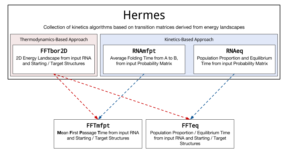
Hermes is organized into three independent directories: (1) FFTbor2D, (2) RNAmfpt, and (3) RNAeq (see Figure 1). These packages compile into both standalone executables and archive files. The archives provide a DRY API which allow the development of novel applications using source from across the Hermes package without having to copy-and-paste relevant functions. We provide two such examples of this in the ext subdirectory: FFTmfpt and FFTeq. These applications are simple C drivers that use functions from FFTbor2D, RNAmfpt and RNAeq to replicate a pipeline of executable calls without having to deal with intermediary data transformation, I/O between calls or slow-down due to a scripting language driver such as Python or R.

3.1 Programs

What follows is a brief overview of the three core applications (FFTbor2D, RNAmfpt, RNAeq), as well as the two extension programs (FFTmfpt, FFTeq). For an exhaustive list of command-line options, please see the corresponding help files.

Given an RNA sequence ${\bf s}$ of length $n$ and two reference structures $A,B$, the algorithm FFTbor2D [35] computes for each $0\leq x,y\leq n$ the Boltzmann probability $P(x,y)=\frac{Z(x,y)}{Z}$ of all structures having base pair distance $x$ to $A$ [resp. $y$ to $B$]. Although the algorithm for the software FFTbor2D is unchanged from that of [35], the software described in this paper has been heavily refactored to provide a user-facing API, homogeneous with the rest of the Hermes suite. As with the rest of Hermes, FFTbor2D makes use of either the Turner 1999 [31] or the later Turner 2004 energy parameters [41], taken respectively from the files rna_turner1999.par and rna_turner2004.par in Vienna RNA Package. FFTbor2D takes as input an RNA sequence ${\bf s}$ and two secondary structures $A,B$ of the input RNA sequence – both given in dot-bracket notation. Alternatively, FFTbor2D can also process a file of RNAs, where data for each RNA appears in the form: FASTA comment, sequence, structure $A$, structure $B$ – each on a separate line. In return, for each RNA, the program returns as output a 2D probability grid whose value at grid position $(x,y)$ is the Boltzmann probability of all secondary structures compatible with ${\bf s}$ having base pair distance $x$ (resp. $y$) from $A$ (resp. $B$).

RNAmfpt computes the mean first passage time (MFPT), sometimes referred to as the hitting time of a Markov chain, by using matrix inversion [33] – see Section 2. The program takes as input a comma separated value (CSV) file containing the non-zero positions and values of a 2D probability grid; i.e. a CSV format file having columns i, j, and p. The first two columns, i and j correspond to the 0-indexed row-ordered position in the rate matrix and the final column p is the probability $p_{i,j}$ of a transition from i to j. From this input, the mean first passage time is constructed by matrix inversion. Because this program was designed with the original intent of handling 2D-probability grids, all vertexes are uniquely identified by index tuples (which conceptually correspond to positioning in a 2D array). However, it is trivial to use this code with both 1D-probability grids such as those produced by FFTbor [36] or arbitrary transition matrices without any change to the underlying implementation. The software additionally provides many options for defining the structure of the graph underlying the Markov chain. Some of these include the option to force a fully connected graph (useful in cases where there is no non-zero path between the start / end state) or to enforce detailed balance. Finally, RNAmfpt also accepts as input the probability transition matrix, a stochastic matrix with row sums equal to $1$, and computes the mean first passage time for the corresponding Markov chain.

RNAeq computes the population proportion of a user-provided structure over arbitrary time units. Like RNAmfpt, this program takes as input a comma separated value (CSV) file containing the non-zero positions and values of a 2D probability grid. From this input a rate matrix is constructed for the underlying Markov process. Alternatively, RNAeq can accept as input an arbitrary rate matrix. Performing spectral decomposition of the column-ordered rate matrix that underlies the corresponding Markov process, RNAeq computes either the equilibrium time or population occupancy frequencies. Additionally, RNAeq can call the Vienna RNA Package program RNAsubopt [46], with a user-specified upper bound to the energy difference with the minimum free energy. With this option, the rate matrix is constructed for the Markov process, whose states consist of all the structures returned by RNAeq, and the equilibrium time or population occupancy frequencies are computed. Due to the time and memory required for this option, we do not expect it to be used except for small sequences.

Beyond these three core applications, Hermes includes two additional programs located in the ext directory, which fulfill more specific roles and highlight the modular nature of the codebase.

FFTmfpt approximates the mean first passage time of a given RNA sequence folding from input structure A to B, by exactly computing the mean first passage time from state $(0,d_{0})$ to state $(d_{0},0)$ in the 2D probability grid obtained from running FFTbor2D. Here, $d_{0}$ is the base pair distance between structures $A,B$, and the MFPT is computed for the Markov chain, whose states are the non-empty 2D probability grid points, and whose transition probabilities are defined by $p_{(x,y),(x^{\prime},y^{\prime})}=\frac{P(x^{\prime},y^{\prime})}{P(x,y)}$. As we report in this paper, given an RNA sequence ${\bf s}$, if $A$ is the empty structure and $B$ the MFE structure of ${\bf s}$, then FFTmfpt output is well correlated with the exact MFPT in folding the empty structure to the MFE structure, where transitions between structures involve the addition or removal of a single base pair.

FFTeq allows an investigator to efficiently estimate population kinetics for a sequence folding between two arbitrary, but fixed, structures. The transition rate matrix underlying the Markov process necessary for eigendecomposition is derived from the 2D-energy landscape. Vertices in the rate matrix represent a subset of structures compatible with the input sequence as modeled by FFTbor2D, which makes the graph size more tractable than structural sampling with RNAsubopt, even with constraints.

Figure 1: Overall organization of Hermes. FFTbor2D, RNAmfpt, and RNAeq are three distinct software packages we have developed, which compile into both standalone executables and archive files, providing a DRY API that allow novel applications development using source from each of the packages, without having to copy-and-paste relevant functions. The applications FFTmfpt and FFTeq are C drivers that use data structures and functions from FFTbor2D, RNAmfpt and RNAeq. FFTmfpt computes the mean first passage time (MFPT) for an RNA secondary structure to fold from an initial structure, such as the empty structure or a given metastable structure, into a target structure, such as the minimum free energy (MFE) structure or possibly the Rfam [20] consensus structure. FFTeq uses spectral decomposition to compute the equilibrium time and the fraction of the population of RNA structures that are equal to a given target structure, as a function of time.

4 Benchmarking results

4.1 Kinetics methods

In this section, we briefly describe the kinetics algorithms used in our comparative study using a benchmarking set of 1,000 small RNAs. Each RNA from the benchmarking set was folded from the initial empty structure to the target minimum free energy structure. Detailed explanations of all kinetics programs and parameters are given in the Appendix.

The kinetics methods benchmarked in Table 1 are MFPT, Equilibrium, FFTmfpt, FFTbor, FFTeq – all computed using Hermes, together with, Kinfold [12], BarrierBasins [45], and RNA2Dfold [30]. The exact data MFPT [resp. Equilibrium] were computed using the Hermes software RNAmfpt [resp. RNAeq] in the following fashion.

The gold standard, MFPT, is obtained by computing the mean first passage time by matrix inverse $(I-P^{-}_{x_{\infty}})^{-1}$ from the transition probability matrix $P$, defined by equation (4) from the ensemble of all secondary structures for each 20-mer in the benchmarking set described in the next section. The platinum standard, Equilibrium, is obtained from the population occupancy frequencies (17), determined by spectral decomposition of the rate matrix, the latter defined by (11) from the ensemble of all secondary structures for each 20-mer in the benchmarking set.

FFTmfpt computes the mean first passage time for the coarse-grained model with macrostates $M(x,y)$, consisting of all secondary structures having base pair distance $x$ from reference structure $A$ and distance $y$ from reference structure $B$. FFTbor2D is used in Hermes to compute the Boltzmann probabilities $p(x,y)=\frac{Z(x,y)}{Z}$ for the coarse-grained model consisting of macrostates $M(x,y)$. Transition probabilities are computed by equation (4), and matrix inversion is used to determine mean first passage time for the coarse-grained model. For comparison purposes, the method FFTbor calls the program FFTbor [36] to compute the Boltzmann probabilities $p(x)=\frac{Z(x)}{Z}$ for the coarse-grained model consisting of macrostates $M(x)$ of all secondary structures having base pair distance $x$ to a given target structure. Mean first passage time is then computed for this model, which is even more coarse-grained than that of FFTmfpt. FFTeq computes the equilibrium time for the coarse-grained model with macrostates $M(x,y)$, consisting of all secondary structures having base pair distance $x$ from reference structure $A$ and distance $y$ from reference structure $B$. As in FFTmfpt, the program FFTbor2D is used to compute the Boltzmann probabilities $p(x,y)=\frac{Z(x,y)}{Z}$ for the coarse-grained model consisting of macrostates $M(x,y)$. The rate matrix is computed by equation (11), then population occupancy frequencies and equilibrium time are computed by equation (7) using spectral decomposition of the rate matrix.

Hastings (Yes\No)	MFPT	Equilibrium	Kinfold	FFTmfpt	RNA2Dfold	FFTbor	BarrierBasins	FFTeq
MFPT	1	0.5683	0.7945	0.5060	0.5110	0.5204	0.5280	0.4472
Equilibrium	0.5798	1	0.7814	0.7043	0.7025	0.5080	0.5979	0.6820
Kinfold	0.7933	0.7507	1	0.7312	0.7358	0.6241	0.6328	0.6445
FFTmfpt	0.6035	0.7935	0.7608	1	0.9980	0.5485	0.8614	0.9589
RNA2Dfold	0.6076	0.7919	0.7655	0.9983	1	0.5584	0.8538	0.9515
FFTbor	0.5416	0.5218	0.6241	0.5748	0.5855	1	0.3450	0.4229
BarrierBasins	0.6346	0.6578	0.6328	0.8310	0.8217	0.3450	1	0.9149
FFTeq	0.5614	0.7916	0.6966	0.9670	0.9590	0.4757	0.8940	1

Table 1: Table of Pearson correlation coefficients for various methods to compute or approximate RNA secondary structure folding kinetics. Lower [resp. upper] triangular entries are with [resp. without] the Hastings correction for Markov chain probability matrices. The methods are: MFPT (mean first passage time, computed by matrix inversion for the Markov chain consisting of all secondary structures, with move allowed between structures differing by one base pair), Equilibrium (equilibrium time, computed by spectral decomposition of a rate matrix comprising all secondary structures to compute population fraction $P(t)$ at time $t$), Kinfold (an implementation of Gillespie’s Algorithm to approximate refolding pathways using an event-based Monte Carlo simulation), FFTmfpt (mean first passage time for Markov chain consisting of “grid point” states $(x,y)$ with probability $P(x,y)=\sum_{S}exp(-E(S)/RT)/Z$, computed by FFTbor2D, where the sum is taken over structures having base pair distance $x$ to the empty structure and $y$ to the MFE structure, RNA2Dfold (mean first passage time, computed as previously explained, but using RNA2Dfold in place of FFTbor2D to compute $P(x,y)$), FFTbor (mean first passage time, computed for the Markov chain consisting of states $0,1,\ldots,n$, for which $P(x)=\sum_{S}\exp(-E(S)/RT)/Z$, where the sum is taken over all secondary structures whose base pair distance is $x$ from the MFE structure), BarrierBasins (equilibrium time, computed using spectral decomposition on the Markov process consisting of “grid point” states output from Barriers), and FFTeq (equilibrium time, computed in the same fashion as BarrierBasins using a Markov process derived from the energy landscape output by FFTbor2D).

Kinetics algorithms developed by other groups and benchmarked in our study are the following: Kinfold [10], BarriersBasin [12, 45], Kinwalker [21]. Below, we give a brief overview of these methods.

Kinfold [10] is an implementation of Gillespie’s Algorithm 2. For benchmarking purposes, we determined the mean first passage time from $10^{4}$ Kinfold simulations, each with an upper bound of $10^{8}$ Monte Carlo steps in order to ensure convergence of each run. BarriersBasin is our name for the method described by Wolfinger et al. [45], which first runs RNAsubopt [12] to obtain an energy-sorted list of secondary structures that contain the empty structure, then computes locally optimal structures, saddle points and macrostate basins of attraction using the program barriers [45]. Subsequently, we use Hermes to determine the equilibrium time for the resulting Markov process whose rate matrix is returned by barriers. Since Kinwalker [21] implements co-transcriptional folding, we found that its correlation with the gold and platinum standards was extremely poor, hence we do not further report the results from our tests with Kinwalker. Programs for the remaining kinetics methods, such as the motion planning method of Tang et al. [39], the stochastic simulation Kinefold [48], etc. from the introduction were either not available, or else it appeared to be difficult/impossible to extract mean first passage times or equilibrium times to compare with the gold and platinum standards.

Finally, Table 1 also includes the method we call here by RNA2Dfold. Given reference structures $A,B$, the RNA2Dfold program [30, 29] computes for each integer $x,y$, the minimum free energy structure and partition function among all secondary structures having base pair distance $x$ to $A$ and $y$ to $B$. FFTbor2D [35] is a much faster program, using the fast Fourier transform, which computes the partition function (but not the minimum free energy structure) over all structures having base pair distance $x$ to $A$ and $y$ to $B$. By the kinetics method dubbed RNA2Dfold, we mean that we applied RNA2Dfold from Vienna RNA Package 2.1.7 [30, 29] in order to obtain probabilities $p(x,y)=\frac{Z(x,y)}{Z}$, and then applied Hermes to compute the mean first passage time for the resulting coarse-grained Markov chain, as in FFTmfpt.

For more detailed description of each kinetics method, please see the Appendix.

4.2 Benchmarking data

In this section, we describe a benchmarking set of 1,000 small RNAs used to benchmark the previously described kinetics methods in a comparative study. To ensure that mean first passage time can be computed from $(I-P^{-}_{x_{\infty}})^{-1}\cdot{\bf e}$ by using matrix inversion, that spectral decomposition of the rate matrix is possible, and to ensure that Kinfold simulations would provide sufficient statistics, we generated a collection of 1,000 random RNA sequences of length 20 nt, each having expected compositional frequency of $1/4$ for A,C,G,U, and each having at most 2,500 distinct secondary structures, such that the minimum free energy is less than or equal to $-5.5$ kcal/mol.

For example, one of the 1,000 sequences is ACGCGACGUGCACCGCACGU with minimum free energy structure .....((((((...)))))) having free energy of $-6.4$ kcal/mol. Statistics for the free energies of the 2,453 secondary structures of this 20-mer are the following: mean is $10.695$, standary deviation is $4.804$, maximum is $25.00$, minimum is $-6.40$. A histogram for the free energy of all secondary structures of ACGCGACGUGCACCGCACGU is depicted in the left panel of Figure 2. The right panel of the same figure depicts the minimum free energy structure of the 54 nt hammerhead type III ribozyme from Peach Latent Mosaic Viroid (PLMVd), discussed later. This secondary structure is identical to the consensus structure from Rfam 11.0 [20].

Figure 2: (Left) Histogram of free energies of secondary structures of ACGCGACGUGCACCGCACGU, which range from $-6.5$ to $+25$ kcal/mol, with mean of $10.695$ kcal/mol. (Right) Minimum free energy structure of the 54 nt Peach Latent Mosaic Viroid (PLMVd) AJ005312.1/282-335, which is identical to the consensus structure from Rfam 11.0 [20]. RNAfold from Vienna RNA Package 2.1.7 with energy parameters from the Turner 1999 model were used, since the minimum free energy structure determined by the more recent Turner 2004 energy parameters does not agree with the Rfam consensus structure – see [7]. Positional entropy, a measure of divergence in the base pairing status at each positions for the low energy ensemble of structures, is indicated by color, using the RNA Vienna Package utility script relplot.pl.

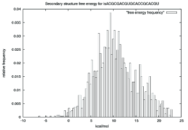
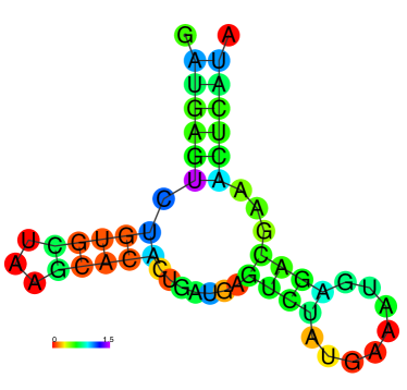
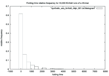
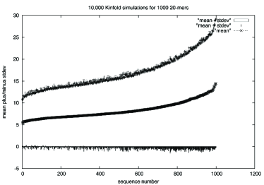
Figure 3 displays the mean and standard deviation for Kinfold simulations of folding time for each of the 1,000 RNA sequences from our benchmarking data. For each sequence, the mean and standard deviation of the time required to fold the empty structure to the MFE structure were computed from 10,000 Kinfold runs, each run with an upper bound of $10^{8}$ Monte Carlo steps, thus ensuring that all simulations converged. The sequences were then sorted by increasing folding time mean. Standard deviation exceeded the mean in $83.9\%$ of the 1,000 cases, indicating the enormous variation between separate Kinfold runs, even for 20 nt RNA sequences having at most 2,500 secondary structures. In our opinion, Kinfold is an expertly crafted implementation of Gillespie’s algorithm for an event driven Monte Carlo simulation of one-step RNA secondary structure folding. From the standpoint of biophysics and physical chemistry, there is no more reliable simulation method, except of course the exact computation of mean first passage time using linear algebra. Nevertheless, the enormous time required for reliable Kinfold estimations and the large standard deviations observed point out the need for a faster method to approximate folding time.

Figure 3: (Left) Histogram of Kinfold folding times for 20-mer CCGAUUGGCG AAAGGCCACC. The mean [resp. standard deviation] of 10,000 runs of Kinfold for this 20-mer is 538.37 [resp. 755.65]. Note the close fit to the exponential distribution, (Right) Mean minus standard deviation ($\mu-\sigma$), mean ($\mu$), and mean plus standard deviation ($\mu+\sigma$) of the logarithm of Kinfold folding times, taken over 10,000 runs for each of the 1,000 sequences from the benchmarking set of 20-mers. For graphical illustration, we have sorted the log folding times in increasing order.

4.3 Correlations

In this section, we display the correlation between (1) the gold standard method MFPT, both with and without the Hastings modification using equations (21) and (25), (2) the platinum standard method Equilibrium, (3) the silver standard method Kinfold, (4) FFTmfpt with and without the Hastings modification using equations (37) and (40), (5) FFTeq which computes equilibrium time for the 2D-grid, (6) RNA2Dfold with and without the Hastings modification using equations (37) and (40). Correlations with [resp. without] the Hastings modification are summarized in the lower [resp. upper] triangular portion of Table 1. It is clear that correlations between the mathematically exact methods MFPT, Equilibrium, and approximation methods Kinfold, FFTmfpt, FFTeq, RNA2Dfold are improved when using the Hastings correction.

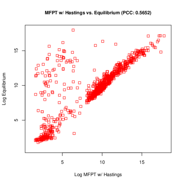
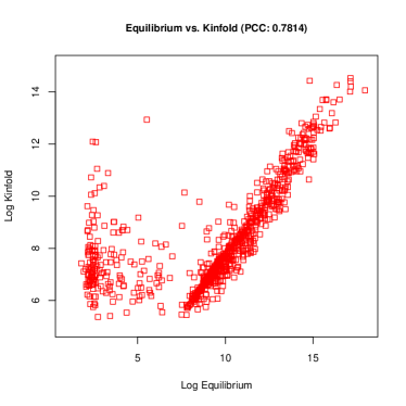
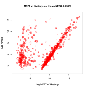
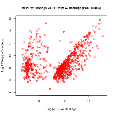
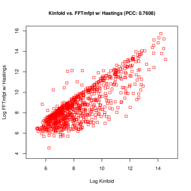
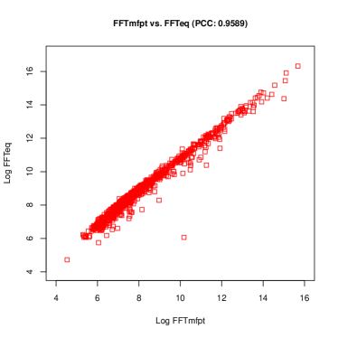
Figures 4, 5, 6 depict scatterplots for kinetics obtained by some of the algorithms above. The left panel of Figure 4 shows a scatter plots for gold standard MFPT versus platinum standard Equilibrium, with correlation value 0.5652. The right panel of the same figure shows a scatter plot for Kinfold versus Equilibrium, with correlation 0.7814. Note the persence of two clusters in this and some of the other scatter plots. Cluster A consists of RNA sequences whose folding time, as determined by MFPT or Equilibrium, is rapid – specifically, the natural logarithm of the MFPT is at most 7.5. Cluster B consists of the remaining RNA sequences, whose folding time is longer than that of cluster A. There are no significant differences between RNA sequences in clusters A and B with respect to GC-content, sequence logo, minimum free energy, number of secondary structures, etc. The left panel of Figure 5 shows the scatter plot for MFPT versus Kinfold, with correlation 0.7933, and the right panel shows the scatter plot for MFPT versus FFTmfpt, with correlation 0.6035. Figure 6 shows scatter plots for FFTmfpt versus Kinfold (left) and for FFTmfpt versus FFTeq (right), with respective correlation values 0.7608 and 0.9589. Kinfold obviously provides a better correlation with the exact value of mean first passage time; however, since the standard deviation of Kinfold runs is as large as the mean, accurate kinetics estimates from Kinfold require prohibitively large computational time – indeed, in [45] reliable kinetics for phe-tRNA from yeast were obtained by 9,000 Kinfold simulations, each for $10^{8}$ steps, requiring 3 months of CPU time on an Intel Pentium 4 running at 2.4 GHz under Linux. Although the correlation value of 0.6035 between MFPT and FFTmfpt is much less than that obtained by Kinfold, the runtime required by our method FFTmfpt is measured in seconds, even for moderate to large RNAs. For this reason, we advocate the use of FFTmfpt in synthetic biology screens to design RNA sequences having certain desired kinetic properties. Once promising candidates are found, it is possible to devote additional computational time to Kinfold simulations for more accurate kinetics.

Figure 4: Scatter plots of the natural logarithm of times from MFPT versus Equilibrium (left) and for Kinfold versus Equilibrium (right).

Figure 5: Scatter plots of the natural logarithm of times from MFPT versus Kinfold (left) and for MFPT versus FFTmfpt (right).

Figure 6: Scatter plots of the natural logarithm of times from Kinfold versus FFTmfpt (left) and for FFTmfpt versus FFTeq (right).

5 Discussion

In this paper, we have introduced the fast, novel RNA kinetics software suite, Hermes, which consists of the three software packages, FFTbor2D, RNAmfpt, and RNAeq, together with two C drivers, FFTmfpt and FFTeq.

Given an RNA sequence ${\bf s}$, FFTbor2D computes the Boltzmann probability $p(x,y)=\frac{Z(x,y)}{Z}$ of secondary structures of ${\bf s}$, whose base pair distance from initial structure $A$ is $x$ and from target structure $B$ is $y$. FFTbor2D is an enhancement of the algorithm described in [35], shown there to run both in theory and in practice much faster than RNA2Dfold [30], since FFTbor2D uses the fast Fourier transform to compute Boltzmann probabilities $p(x,y)$ by polynomial interpolation.

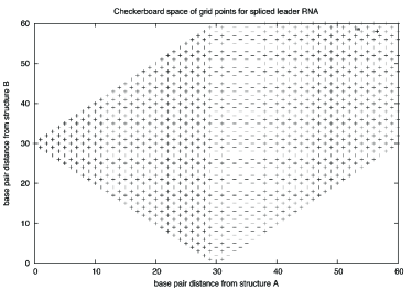
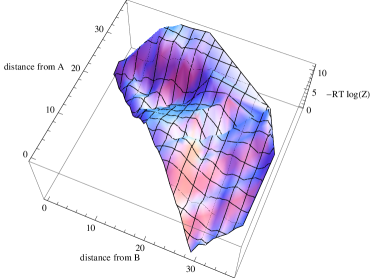
RNAmfpt computes the mean first passage time for the coarse-grained Markov chain, consisting of the macrostates $M(x,y)$ of all secondary structures, whose base pair distance is $x$ [resp. $y$] from initial structure $A$ [resp. target structure $B$]. Given an initial state $A=(x_{0},y_{0})$, a target state $B=(x_{1},y_{1})$, and the 2D grid of positions $(x,y)$ and probabilities $p(x,y)$ as computed by FFTbor2D and illustrated in Figure 7, RNAmfpt computes the mean first passage time, taken over all paths from $(x_{0},y_{0})$ to $(x_{1},y_{1})$. Alternatively, RNAmfpt can take as input the probability transition matrix $P$ for an arbitary finite Markov chain $\mathbb{M}$, and subsequently determines the mean first passage time by computing the inverse $(I-P^{-}_{x_{\infty}})^{-1}=\displaystyle\sum_{k=0}^{\infty}(P^{-}_{x_{\infty}})^{k}$.

As in the case of RNAmfpt, RNAeq computes the equilibrium time for the coarse-grained Markov process, consisting of the macrostates $M(x,y)$ of all secondary structures, whose base pair distance is $x$ [resp. $y$] from initial structure $A$ [resp. target structure $B$]. Given an initial state $A=(x_{0},y_{0})$, a target state $B=(x_{1},y_{1})$, and the 2D grid of positions $(x,y)$ and probabilities $p(x,y)$ as returned by FFTbor2D and illustrated in Figure 7, RNAeq computes the population occupancy frequencies $P(t)=(P_{1}(t),\ldots,P_{n}(t))$ by using spectral decomposition, and then determines the equilibrium time. Alternatively, given an input RNA sequence RNAeq calls RNAsubopt [47] to generate structures within a user-specified energy bound (or to sample a user-specified number of structures from the low energy ensemble). RNAeq subsequently computes the rate matrix and computes population occupancy frequencies and equilibrium time. RNAeq can additionally take as input the rate matrix $R$ for an arbitary finite Markov process $\mathbb{M}$, and then compute population occupancy frequencies and the equilibrium time.

Given an RNA sequence, the C-drivers FFTmfpt and FFTeq respectively compute the mean first passage time (MFPT) and equilibrium time (ET) for the coarse-grained Markov chain on the macrostates $M(x,y)$ of all secondary structures whose base pair distance is $x$ [resp. $y$] from initial structure $A$ [resp. target structure $B$]. This is done by calling FFTbor2D, in order to determine the 2D probabilities, from which the transition probability matrix or respectively rate matrix are determined, and then calling RNAmfpt or respectively RNAeq.

Figure 7: (Left) As first pointed out in [30], the set of grid points $(x,y)$, for which a secondary structure $S$ has base pair distance $x$ from reference structure $A$ and base pair distance $y$ from reference structure $B$, forms a kind of checkerboard image. For the 56 nt spliced leader RNA from L. collosoma [28], with sequence AACUAAAACA AUUUUUGAAG AACAGUUUCU GUACUUCAUU GGUAUGUAGA GACUUC, and reference structure $A$ given by ..((...((((((..(((((.((((...)))).)))))..))).)))..))....., and reference structure $B$ given by .......................((((((((((((.....)))))..))))))).., we obtain the possible grid points depicted in this figure. The $x$-axis (resp. $y$-axis) represents base pair distance between initial structure $A$ (resp. target structure $B$). Consideration of the triangle inequality and parity condition (see text) ensure that partition function values $Z(x,y)$ and Boltzmann probabilities $p(x,y)=\frac{Z(x,y)}{Z}$ are zero for all non-grid points $(x,y)$. (Right) 2D projection of energy landscape for Spliced Leader (SL) RNA from Leptomonas collosoma, in which the $z$-axis represents the ensemble free energy $-RT\log Z(x,y)$, where $Z(x,y)$ is computed in FFTbor2D by $Z_{x,y}=p(x,y)\cdot Z$. Low energy positions $(x,y)$ correspond to high Boltzmann probability positions. Image taken from [35].

Using functions from Gnu Scientific Library (GSL) http://www.gnu.org/software/gsl/, mean first passage time (MFPT) is computed by matrix inversion $(I-P^{-}_{x_{\infty}})^{-1}$ from the transition probability matrix $P$, while equilibrium time (ET) is computed by spectral decomposition of the rate matrix. Hermes makes available a variety of novel RNA folding kinetics methods: MFPT (via RNAmpft), Equilibrium (via RNAeq), FFTmfpt, and FFTeq. Using a collection of 1,000 randomly generated 20-mers having at most 2,500 secondary structures, using Hermes the gold standard mean first passage time and platinum standard equilibrium time were computed for each sequence. Pearson correlation was then computed between the folding times of all the methods of Hermes, along with the current state-of-the-art kinetics programs Kinfold [10], BarrierBasins [45], Kinwalker [21].

Kinfold is an implementation of the Gillespie algorithm [22], which essentially samples from an exponential distribution of folding times, hence Kinfold mean and standard deviation are approximately equal – see Figure 3. Elementary considerations from statistics indicate that for our benchmarking set of 20-mers, the minimum sample size $n=\left(\frac{z_{\alpha/2}\cdot\sigma}{E}\right)^{2}$ ranges from 937,712 to 23,289,310 for us to have a confidence level of 95% that the average of $n$ Kinfold runs differs from the real folding time by at most 100 steps. Since this is the case for tiny sequences of 20 nt, it follows that only enormous computation time can provide reliable folding times for larger sequences when using Kinfold.

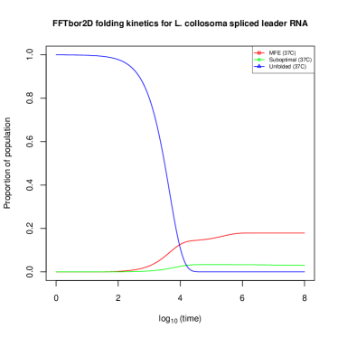
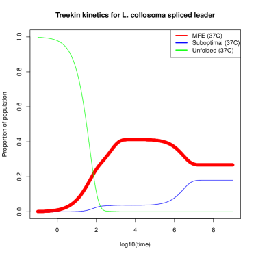
Since the state-of-the-art software Kinfold, which implements Gillespie’s algorithm, cannot return statistically significant folding times unless significant computation time is allotted, it is natural to turn to coarse-grained models, as done by Wolfinger et al. [45] and by Tang et al. [39]. The software of Tang et al. appears not to be available. Concerning the method of Wolfinger et al. (called BarrierBasins in our benchmarking), there is now a web server available, which runs RNAsubopt [46] to generate all secondary structures within a user-specified energy range, then runs barriers [12] to generate basins of attraction around a user-specified number of locally optimal structures, and then runs treekin on the output of barriers. The program treekin performs some of the same operations as Hermes, by computing population occupation frequencies by spectral decomposition. Nevertheless it would require a user to write scripts and perform several manual steps, in order to determine the equilibrium time for an input RNA sequence, with respect to the macrostate Markov process of [45]. In addition, because barriers computes basins of attraction by utilizing the output of RNAsubopt, estimating kinetics for the refolding of an RNA molecule from the empty structure requires exhaustive enumeration of all suboptimal structures having non-positive free energy. Figure 8 depicts some population occupancy curves for the 56 nt spliced leader RNA from L. collorosoma, a known conformational switch experimentally investigated in [28], a determined by Hermes (left panel) and barriers with treekin (right panel).

In contrast, Hermes is a fully automated software suite which computes mean first passage time and equilibrium time with respect to the coarse-grained model that consists of macrostates $M(x,y)$ of all structures having base pair distance $x$ to initial structure $A$ and $y$ to target structure $B$. Additionally, Hermes provides a number of other functionalities useful for RNA kinetics. Since Hermes includes FFTbor2D, which uses the fast Fourier transform to compute probabilities $p(x,y)$ of macrostates $M(x,y)$, the resulting coarse-grained kinetics computations are extremely fast. Hermes can provide approximate refolding kinetics for RNA sequences that are larger than those which other software can handle. As well, the correlation values shown in Table 1 demonstrate that Hermes can be used for fast, approximate and relatively accurate RNA kinetics in a pipeline to select promising candidates in the design of RNA sequences.

Figure 8: (Left) Population occupancy curves computed with FFTeq for the 56 nt conformational switch L. collosoma spliced leader RNA, with sequence AACUAAAACA AUUUUUGAAG AACAGUUUCU GUACUUCAUU GGUAUGUAGA GACUUC. The dot bracket format for the MFE structure, as computed by version 2.1.7 of RNAfold -d0, is .......................((((((((((((.....)))))..))))))).. with free energy $-8.6$ kcal/mol, while that of the the alternate suboptimal structure is ..((...((((((..(((((.((((...)))).)))))..))).)))..))..... with free energy $-7.5$ kcal/mol. In the case of the MFE structure, the equilibrium occupancy $P(t_{\infty})$, which Hermes approximates as $0.17893806$ should equal the Boltzmann probability $0.17909227$, since the MFE structure is the only structure at distance $x_{0}$ [resp. $y_{0}$] from the reference structures $A$ (empty structure) [resp. $B$ (MFE structure)]. As well, if there are few other low energy structures at the same base pair distance $x_{1}$ [resp. $y_{1}$] from $A$ [resp. $B$] as that of the alternate suboptimal structure, then we expect that the occupancy probability $0.03003426$ for the $(x_{1},y_{1})$ be approximately the Boltzmann probability $0.03005854$ of the alternate structure. (Right) Population occupancy curves computed for L. collosoma spliced leader RNA, computed using RNA Vienna Package with the following commands: RNAsubopt -d0 -s -e 17 > foo.sub, barriers -M noShift --max=1000 --rates --minh 0.1 < foo.sub > foo.bar, treekin --method I --p0 940=1 --ratesfile rates.out < foo.bar > out.bar, where the value 940 indicates the empty structure appearing as the 940^th structure in the sorted file foo.bar of 1,000 locally optimal structures. The red curve corresponds to the basin of attraction around the minimum free energy structure. At equilibrium, the Boltzmann probability of this basin is between 0.3 and 0.4, a value substantially greater than the Boltzmann probability of the minimum free energy structure itself, which is $\approx 0.1791$ as shown in the left panel.

Finally, we mention an application of Hermes to recent data from Dotu et al. [7], which describes the first purely computational design of functional synthetic hammerhead type III ribozymes, experimentally shown to cleave in vitro. For the tiny data set of 10 synthetic ribozymes, we ran FFTmfpt to determine the log(MFPT) of folding from the empty structure to the target consensus structure of Peach Mosaic Latent Viroid (PMLVd), shown in Figure 2. We determined a Pearson correlation of $0.4796$ [resp. $0.5322$] between the logarithm of the mean first passage time [resp. equilibrium time], as computed by FFTmfpt [resp. RNAeq] and the cleavage rate, using the experimentally measured cleavage rate of 10 synthetic hammerhead ribozymes (data from [7]). These correlation values seem surprising, since we had expected that rapidly folding hammerheads (low values of MFPT and ET) might be associated with fast cleavage. The correlation values suggest instead that perhaps the longer a hammerhead requires to fold into its functional secondary structure, shown in Figure 2, the more rapid its cleavage. If this observation can be experimentally validated on a large set of hammerheads, then the insight could be potentially important for RNA design, an area of synthetic biology.

6 Acknowledgements

We would like to thank Ivan Dotu, for the suggestion of checking the folding kinetics of the synthetic hammerheads in [7]. Some of the work described in this paper was done while PC visited Niles Pierce at the California Institute of Technology, Knut Reinert at the Free University of Berlin and Martin Vingron at the Max Planck Institute for Molecular Genetics. Warm thanks are due to all three persons. The research was funded by National Science Foundation grant DBI-1262439, the Guggenheim Foundation and Deutscher Akademischer Austauschdienst. Any opinions, findings, and conclusions or recommendations expressed in this material are those of the authors and do not necessarily reflect the views of the National Science Foundation.

Appendix

Kinetics methods in benchmarking

In this section, we describe the kinetics algorithms used in our comparative study on a benchmarking set of 1000 small RNAs. The kinetics algorithms we consider are the following: MFPT, Equilibrium, Kinfold [10], FFTmfpt, FFTeq, RNA2Dfold, FFTbor1D, BarrierBasins [45], Kinwalker [21]. Our software suite Hermes introduces the new methods MFPT, Equilibrium, FFTmfpt, FFTeq (along with RNA2Dfold and FFTbor1D through the utility programs RNAmfpt and RateEq). Although all these methods allow one to compute folding kinetics from an arbitrary initial structure to an arbitrary final structure, in the benchmarking comparison, we consider only folding from the empty structure to the MFE structure.

MFPT

: Given RNA sequence ${\bf s}$ and secondary structure $x$, let $N(x)$ denote the set of neighboring secondary structures of ${\bf s}$, whose base pair distance with $x$ is one. Define the Markov chain $\mathcal{M}({\bf s})=(SS({\bf s}),P)$, where $SS({\bf s})$ denotes the set of all secondary structures of ${\bf s}$, $p^{*}(x)$ is the stationary probability of structure $x$, defined by $p^{*}(x)=\exp(-E(x)/RT)/Z$, $Z=\sum_{x}\exp(-E(x)/RT)$, and the transition probability matrix $P=(p_{x,y})$ is defined either with or without the Hastings modification as follows.

With the Hastings modification,

$$p_{x,y}=\left\{\begin{array}[]{ll}\frac{1}{|N(x)|}\cdot\min(1,\frac{p^{*}(y)}{p^{*}(x)}\cdot\frac{N(x)}{N(y)})&\mbox{if $y\in N(x)$}\\ 0&\mbox{if $x\neq y,y\not\in N(x)$}\\ 1-\sum_{\begin{subarray}{c}z\in N(x)\end{subarray}}p_{x,z}&\mbox{if $x=y$}\\ \end{array}\right.$$ (21)

Without the Hastings modification,

$$p_{x,y}=\left\{\begin{array}[]{ll}\frac{1}{|N(x)|}\cdot\min(1,\frac{p^{*}(y)}{p^{*}(x)})&\mbox{if $y\in N(x)$}\\ 0&\mbox{if $x\neq y,y\not\in N(x)$}\\ 1-\sum_{\begin{subarray}{c}z\in N(z)\end{subarray}}p_{x,z}&\mbox{if $x=y$}\\ \end{array}\right.$$ (25)

The exact value of mean first passage time (MFPT) can be computed as follows. Let $x_{0}$ [resp. $x_{\infty}$] denote the empty structure [resp. MFE structure] for sequence ${\bf s}$ (here we have implicitly identified integer indices with secondary structures). Let $\widetilde{P}_{x_{\infty}}$ be the matrix obtained from $P$ by removal of the row and column with index $x_{\infty}$, and $I$ denote the $(n-1)\times(n-1)$ identity matrix, where $n=|SS({\bf s})|$ is the number of secondary structures of ${\bf s}$. Let $e$ denote the vector of size $n-1$, each of whose coordinates is $1$. It is well-known [33] that for each $k\neq x_{\infty}$, the $k$th coordinate of the vector $(I-\widetilde{P}_{x_{\infty}})^{-1}\cdot{\bf e}$ is exactly equal to the mean first passage time from the structure with index $k$ to the target structure $x_{\infty}$. In particular, the MFPT from the empty structure to the MFE structure is computable by applying matrix inversion from GSL. Since this computation of the mean first passage time is mathematically exact, we consider that MFPT to be the gold standard value for RNA folding kinetics.

Equilibrium

: Define the continuous Markov process $\mathcal{M}=(SS({\bf s}),R)$, where $R$ is the rate matrix defined by

$$k_{x,y}=\left\{\begin{array}[]{ll}\min(1,\frac{p^{*}(y)}{p^{*}(x)})&\mbox{if $y\in N(x)$}\\ 0&\mbox{if $x\neq y,y\not\in N(x)$}\\ -\sum_{\begin{subarray}{c}z\in N(z)\end{subarray}}p_{x,z}&\mbox{if $x=y$}\\ \end{array}\right.$$ (29)

Clearly the rate matrix satisfies detailed balance; i.e. $p^{*}(x)\cdot k_{x,y}=p^{*}(y)\cdot k_{y,x}$ for all distinct $x,y\in SS({\bf s})$. In fact, the rate matrix for Markov processes is usually defined as above, precisely to ensure detailed balance, which then implies that all eigenvalues of the rate matrix are real, thus permitting explicit solution of the population occupancy frequency for all states.

Kinfold

: Version 1.3 of Kinfold [13], from the Vienna RNA Package (version 2.1.7) was run with the following flags:

Kinfold --dangle 0 --met --noShift --logML --num=10000 --time=100000000

Kinfold 1.3 uses the Turner2004 energy model, and the flags in the command line indicate that dangles are not considered, that the Metropolis rule is employed (rather than the Kawasaki rule), that moves consist only of the addition or removal of a single base pair, that the number of repeated Monte Carlo runs per sequence is $10^{4}$, and that each run has an upper bound of $10^{8}$ steps. For the RNA sequences of 20 nt used in our benchmarking set, with these flags, every run for every sequence properly terminated in the target minimum free energy structure. For each sequence, the mean (and standard deviation) of $10^{4}$ runs was determined; this mean is deemed the mean first passage time, as estimated by Kinfold. Implemented in the Vienna RNA Package 2.1.7, Kinfold is what may be considered the silver standard value for folding kinetics, since exact determination of mean first passage time, using matrix inversion is impossible except for sequences not having more than several thousand secondary structures. However, due to the stochastic nature of the Gillespie algorithm implemented by Kinfold, very many runs with very long run times are required to obtain a reasonable approximation of the MFPT.

FFTmfpt

: Given an RNA sequence ${\bf s}$, the algorithm FFTbor2D [35] computes the probabilities $p(x,y)=\frac{Z(x,y)}{Z}$ of secondary structures of ${\bf s}$ to have base pair distance $x$ [resp. $y$] to secondary structure $A$ [resp. $B$], where $A$ is taken to be the empty structure and $B$ is the MFE structure. Let $d_{BP}(S,T)$ denote the base pair distance between structures $S,T$. Then $Z(x,y)=\sum_{S}\exp(-E(S)/RT)$, where the sum is over structures $S$, such that $d_{BP}(A,S)=x$, and $d_{BP}(B,S)=y$; as well the partition function $Z=\sum_{S}\exp(-E(S)/RT)$, where the sum is over all seconddary structures $S$ of the sequence ${\bf s}$.

Let $d_{0}=d_{BP}(A,B)$, the base pair distance between initial structure $A$ and target structure $B$. Let $n$ denote the length of sequence ${\bf s}$. Define the Markov chain $\mathcal{M}_{1}({\bf s})=(Q_{1},P_{1})$, where

$$Q_{1} = \{(x,y):0\leq x,y\leq n,(x+y\bmod 2)=(d_{0}\bmod 2),$$

$$(d_{0}\leq x+y),(x\leq d_{0}+y),(y\leq d_{0}+x).Triangleinequality$$

For reference, we say that the parity condition holds for $(x,y)$ if

$$(x+y\bmod 2)=(d_{0}\bmod 2).$$ (31)

We say that the triangle inequality holds for $(x,y)$ if

$$(d_{0}\leq x+y),(x\leq d_{0}+y),(y\leq d_{0}+x)$$ (32)

Figure 7 displays the space of possible grid points $(x,y)$ for spliced leader RNA from L. collosoma with two reference structures.

Since we allow transitions between secondary structures that differ by exactly one base pair, Markov chain transitions are allowed to occur only between states $(x,y),(u,v)\in Q_{1}$, such that $u=x\pm 1$, $v=y\pm 1$. However, we have found that for some RNA sequences, there is no non-zero probability path from $(0,d_{0})$ to $(d_{0},0)$ (corresponding to a folding pathway from structure $A$ to $B$).

To address this situation, we proceed as follows. Let $\epsilon=10^{-8}$ and for all $(x,y)\in Q_{1}$, modify probabilities $p(x,y)$ by

$$p(x,y) = \frac{p(x,y)+\epsilon/|Q_{1}|}{1+\epsilon}.$$ (33)

This operation corresponds to adding the negligeable value of $\epsilon=10^{-8}$ to the total probability, thus ensuring that there are paths of non-zero probability between any two states. After this $\epsilon$-modification and renormalization, when using the Hastings modification, the transition probabilities $P((u,v)|(x,y))$ are given by

$$P((u,v)|(x,y))=\left\{\begin{array}[]{ll}\frac{1}{|N(x,y)|}\cdot\min(1,\frac{p(u,v)}{p(x,y)}\cdot\frac{N(x,y)}{N(u,v)})&\mbox{if $(u,v)\in N(x,y)$}\\ 0&\mbox{if $(x,y)\neq(u,v)\mbox{ and }(u,v)\not\in N(x,y)$}\\ 1-\sum_{\begin{subarray}{c}(u,v)\in N(x,y)\end{subarray}}P((u,v)|(x,y))&\mbox{if $(x,y)=(u,v)$}\\ \end{array}\right.$$ (37)

Here the set $N(x,y)$ of adjacent neighbors is defined by $N(x,y)=\{(u,v)\in Q_{1}:u=x\pm 1,v=y\pm 1\}$, and the stationary probability $p(x,y)$ is obtained from FFTbor2D.

Without the Hastings modification, the transition probabilities $P((u,v)|(x,y))$ are instead given by

$$P((u,v)|(x,y))=\left\{\begin{array}[]{ll}\frac{1}{|N(x,y)|}\cdot\min(1,\frac{p(u,v)}{p(x,y)})&\mbox{if $(u,v)\neq(x,y)$}\\ 1-\sum_{\begin{subarray}{c}(u,v)\neq(x,y)\end{subarray}}P((u,v)|(x,y))&\mbox{if $(x,y)=(u,v)$}\\ \end{array}\right.$$ (40)

FFTeq

: This method consists of computing the equilibrium time from the master equation for the coarse-grain Markov process $\mathcal{M}=(Q_{1},R)$, where $Q_{1}$ is defined in equation (FFTmfpt), and the rate matrix $R=(k((x,y),(u,v)))$ is defined by

$$k((x,y),(u,v))=\left\{\begin{array}[]{ll}\min(1,\frac{p(u,v)}{p(x,y)})&\mbox{if $(u,v)\neq(x,y)$}\\ 1-\sum_{\begin{subarray}{c}(u,v)\neq(x,y)\end{subarray}}P((u,v)|(x,y))&\mbox{if $(x,y)=(u,v)$}\\ \end{array}\right.$$ (43)

Equilibrium time is then computed for this Markov process.

RNA2Dfold

: The program RNA2Dfold of Vienna RNA Package 2.1.7 was run to compute the probabilities $p(x,y)=\frac{Z(x,y)}{Z}$ of secondary structures of ${\bf s}$ to have base pair distance $x$ [resp. $y$] to secondary structure $A$ [resp. $B$], where $A$ is the empty structure and $B$ is the minimum free energy structure. As in the case for FFTbor2D, Figure 7 displays the checkerboard image of possible grid points $(x,y)$ for spliced leader RNA from L. collosoma with two reference structures.

The probabilities $p(x,y)$ were then $\epsilon$-modified and normalized, as in the description above for FFTeq, and the mean first passage time for the Markov chain $\mathcal{M}_{2}({\bf s})=(Q_{1},P_{2})$ is computed, where $P_{2}$ is the transition probability matrix, as in FFTbor2D, with the exception that $p(x,y)$ is initially obtained from RNA2Dfold, rather than FFTbor2D.

When working with RNA2Dfold, it is more accurate to compute transition probabilities of the form

$$P((u,v)|(x,y))=\frac{1}{N(x,y)}\cdot\min(1,\exp(-\frac{E(u,v)-E(x,y)}{RT}))$$

instead of the mathematically equivalent form

$$P((u,v)|(x,y))=\frac{1}{N(x,y)}\cdot\min(1,\frac{p(u,v)}{p(x,y)})$$

for reasons due solely to numerical precision. However, since it is necessary to perform $\epsilon$-modification and renormalization of transition probabilities, one is led to modify the free energy in the following manner.

Letting $G$ denote ensemble free energy $-RT\ln Z$, as computed by RNAfold and RNA2Dfold,

$$p = \exp(-E/RT)/\exp(-G/RT)$$

$$= \exp(-[E-G]/RT)$$

hence it follows that $-RT\ln p=E-G$ and $E=G-RT\ln p$.

By adding $\epsilon=10^{-8}/|Q_{1}|$ to every probability in every state $(x,y)\in Q_{1}$, the $\epsilon$-modified and renormalized probability corresponding to $p$ is $\frac{p+\epsilon/|Q_{1}|}{1+\epsilon}$ and so the corresponding new energy term is

$$Enew = G-RT\ln(\frac{p+\epsilon}{1+\epsilon\cdot|Q_{1}|}).$$ (44)

It follows that we are forced to use probabilities in any case, and so we encounter the above-mentioned loss of accuracy.

BarrierBasins

: Using the --rate flag for the program barriers [12], Wolfinger et al. [45] computed the rate matrix for a Markov process, whose states are the basins of attraction around locally optimal secondary structures. Subsequently, using Treekin, the authors displayed population occupancy curves for certain macrostates (basins of attraction) containing specific structures of interest. Since this method was not given a name by the authors, we let BarrierBasins denote the equilibrium time for the Markov process just described.

Kinwalker

: Kinwalker was used with default settings. However, since Kinwalker models co-transcriptional folding of RNA, its correlation was extremely poor with all other methods, which do model refolding, rather than co-transcriptional folding (data not shown). For this reason, we do not display the results with Kinwalker.

References

- [1] J. W. Anderson, P. A. Haas, L. A. Mathieson, V. Volynkin, R. Lyngso, P. Tataru, and J. Hein. Oxfold: kinetic folding of RNA using stochastic context-free grammars and evolutionary information. Bioinformatics, 29(6):704–710, March 2013.
- [2] C. B. Anfinsen. Principles that govern the folding of protein chains. Science, 181:223–230, 1973.
- [3] I. Aviram, I. Veltman, A. Churkin, and D. Barash. Efficient procedures for the numerical simulation of mid-size RNA kinetics. Algorithms. Mol. Biol., 7(1):24, 2012.
- [4] A. Bujotzek, M. Shan, R. Haag, and M. Weber. Towards a rational spacer design for bivalent inhibition of estrogen receptor. J. Comput. Aided. Mol. Des., 25(3):253–262, March 2011.
- [5] P. Clote and R. Backofen. Computational Molecular Biology: An Introduction. John Wiley & Sons, 2000. 279 pages.
- [6] L. V. Danilova, D. D. Pervouchine, A. V. Favorov, and A. A. Mironov. RNAKinetics: a web server that models secondary structure kinetics of an elongating RNA. J. Bioinform. Comput. Biol., 4(2):589–596, April 2006.
- [7] I. Dotu, J.A. Garcia-Martin, B.L. Slinger, V. Mechery, M.M. Meyer, and P. Clote. Complete RNA inverse folding: computational design of functional hammerhead ribozymes. Nucleic Acids Res., 2014. in press.
- [8] C. Fasting, C. A. Schalley, M. Weber, O. Seitz, S. Hecht, B. Koksch, J. Dernedde, C. Graf, E. W. Knapp, and R. Haag. Multivalency as a chemical organization and action principle. Angew. Chem. Int. Ed. Engl., 51(42):10472–10498, October 2012.
- [9] C. Flamm. Kinetic folding of RNA, 1998.
- [10] C. Flamm, W. Fontana, I.L. Hofacker, and P. Schuster. RNA folding at elementary step resolution. RNA, 6:325–338, 2000.
- [11] C. Flamm, I. L. Hofacker, S. Maurer-Stroh, P. F. Stadler, and M. Zehl. Design of multistable RNA molecules. RNA., 7(2):254–265, February 2001.
- [12] C. Flamm, I.L. Hofacker, P.F. Stadler, and M. Wolfinger. Barrier trees of degenerate landscapes. Z. Phys. Chem., 216:155–173, 2002.
- [13] Christoph Flamm, Walter Fontana, Ivo L. Hofacker, and Peter Schuster. RNA folding at elementary step resolution. RNA, 6:325–338, 2000.
- [14] Joel N. Franklin. Matrix Theory. Dover Publications, Mineola, New York, 2000. 292 pages.
- [15] E. Freyhult, V. Moulton, and P. Clote. Boltzmann probability of RNA structural neighbors and riboswitch detection. Bioinformatics, 23(16):2054–2062, August 2007.
- [16] E. Freyhult, V. Moulton, and P. Clote. RNAbor: a web server for RNA structural neighbors. Nucleic. Acids. Res., 35(Web):W305–W309, July 2007.
- [17] Matteo Frigo and Steven G. Johnson. The design and implementation of FFTW3. Proceedings of the IEEE, 93(2):216–231, 2005. Special issue on “Program Generation, Optimization, and Platform Adaptation”.
- [18] J. A. Garcia-Martin, P. Clote, and I. Dotu. RNAiFold: a web server for RNA inverse folding and molecular design. Nucleic. Acids. Res., 41(Web):W465–W470, July 2013.
- [19] J.A. Garcia-Martin, P. Clote, and I. Dotu. RNAiFold: A constraint programming algorithm for RNA inverse folding and molecular design. J Bioinform Comput Biol, 11(2):1350001, 2013. in press.
- [20] P. P. Gardner, J. Daub, J. Tate, B. L. Moore, I. H. Osuch, S. Griffiths-Jones, R. D. Finn, E. P. Nawrocki, D. L. Kolbe, S. R. Eddy, and A. Bateman. Rfam: Wikipedia, clans and the ”decimal” release. Nucleic. Acids. Res., 39(Database):D141–D145, January 2011.
- [21] M. Geis, C. Flamm, M. T. Wolfinger, A. Tanzer, I. L. Hofacker, M. Middendorf, C. Mandl, P. F. Stadler, and C. Thurner. Folding kinetics of large RNAs. J. Mol. Biol., 379(1):160–173, May 2008.
- [22] D.T. Gillespie. A general method for numerically simulating the stochastic time evolution of coupled chemical reactions. J Comp Phys, 22(403):403–434, 1976.
- [23] AR. Gruber, R. Lorenz, SH. Bernhart, R. Neubock, and IL. Hofacker. The vienna rna websuite. Nucleic Acids Research, 36:70–74, 2008.
- [24] C. Hobartner and R. Micura. Bistable secondary structures of small RNAs and their structural probing by comparative imino proton NMR spectroscopy. J. Mol. Biol., 325(3):421–431, January 2003.
- [25] L. M. Hochrein, M. Schwarzkopf, M. Shahgholi, P. Yin, and N. A. Pierce. Conditional Dicer substrate formation via shape and sequence transduction with small conditional RNAs. J. Am. Chem. Soc., 135(46):17322–17330, November 2013.
- [26] J. Huang and B. Voss. Analysing RNA-kinetics based on folding space abstraction. BMC. Bioinformatics, 15:60, 2014.
- [27] D. Lai, J. R. Proctor, and I. M. Meyer. On the importance of cotranscriptional RNA structure formation. RNA., 19(11):1461–1473, November 2013.
- [28] K.A. Lecuyer and D.M. Crothers. The Leptomonas collosoma spliced leader RNA can switch between two alternate structural forms. Biochemistry, 32(20):5301–5311, 1993.
- [29] R. Lorenz, S. H. Bernhart, C. Honer Zu Siederdissen, H. Tafer, C. Flamm, P. F. Stadler, and I. L. Hofacker. Viennarna Package 2.0. Algorithms. Mol. Biol., 6:26, 2011.
- [30] R. Lorenz, C. Flamm, and I.L. Hofacker. 2D projections of RNA folding landscapes. In I. Grosse, S. Neumann, S. Posch, F. Schreiber, and P.F. Stadler, editors, German Conference on Bioinformatics 2009, volume 157 of Lecture Notes in Informatics, pages 11–20, 2009.
- [31] D.H. Matthews, J. Sabina, M. Zuker, and D.H. Turner. Expanded sequence dependence of thermodynamic parameters improves prediction of RNA secondary structure. J. Mol. Biol., 288:911–940, 1999.
- [32] N. Metropolis, A.W. Rosenbluth, M.N. Rosenbluth, A.H. Teller, and E. Teller. Equation of state calculations by fast computing machines. J. Chem. Phys., 21:1087–1092, 1953.
- [33] C.D. Meyer. The role of the group inverse in the theory of finite Markov chains. SIAM Rev., 17(46):443–464, 1975.
- [34] S.R. Morgan and P.G. Higgs. Barrier heights between ground states in a model of RNA secondary structure. J. Phys. A: Math. Gen., 31:3153–3170, 1998.
- [35] E. Senter, I. Dotu, and P. Clote. RNA folding pathways and kinetics using 2D energy landscapes. J Math Biol, 2014.
- [36] E. Senter, S. Sheikh, I. Dotu, Y. Ponty, and P. Clote. Using the fast fourier transform to accelerate the computational search for RNA conformational switches. PLoS. One., 7(12):e50506, 2012.
- [37] B. A. Shapiro, D. Bengali, W. Kasprzak, and J. C. Wu. RNA folding pathway functional intermediates: their prediction and analysis. J. Mol. Biol., 312(1):27–44, September 2001.
- [38] X. Tang, B. Kirkpatrick, S. Thomas, G. Song, and N. M. Amato. Using motion planning to study RNA folding kinetics. J. Comput. Biol., 12(6):862–881, 2005.
- [39] X. Tang, S. Thomas, L. Tapia, D. P. Giedroc, and N. M. Amato. Simulating RNA folding kinetics on approximated energy landscapes. J. Mol. Biol., 381(4):1055–1067, September 2008.
- [40] C. Thachuk, J. Manuch, A. Rafiey, L. A. Mathieson, L. Stacho, and A. Condon. An algorithm for the energy barrier problem without pseudoknots and temporary arcs. Pac Symp Biocomput., 0(O):O, 2010:108-19.
- [41] D. H. Turner and D. H. Mathews. NNDB: the nearest neighbor parameter database for predicting stability of nucleic acid secondary structure. Nucleic. Acids. Res., 38(Database):D280–D282, January 2010.
- [42] J. R. Vieregg and I. Tinoco. Modelling RNA folding under mechanical tension. Mol. Phys., 104(8):1343–1352, April 2006.
- [43] M. Wachsmuth, S. Findeiss, N. Weissheimer, P. F. Stadler, and M. Morl. De novo design of a synthetic riboswitch that regulates transcription termination. Nucleic. Acids. Res., 41(4):2541–2551, February 2013.
- [44] M.S. Waterman. Introduction to Computational Biology: Maps, Sequences and Genomes. Chapman & Hall/CRC Press, 1995.
- [45] M. Wolfinger, W.A. Svrcek-Seiler1, C. Flamm, and P.F. Stadler. Efficient computation of RNA folding dynamics. J Phys. A: Math. Gen., 37:4731–4741, 2004.
- [46] S. Wuchty, W. Fontana, I. L. Hofacker, and P. Schuster. Complete suboptimal folding of RNA and the stability of secondary structures. Biopolymers, 49:145–165, 1999.
- [47] S. Wuchty, W. Fontana, I.L. Hofacker, and P. Schuster. Complete suboptimal folding of RNA and the stability of secondary structures. Biopolymers, 49:145–164, 1999.
- [48] A. Xayaphoummine, T. Bucher, and H. Isambert. Kinefold web server for RNA/DNA folding path and structure prediction including pseudoknots and knots. Nucleic. Acids. Res., 33(Web):W605–W610, July 2005.
- [49] J. N. Zadeh, B. R. Wolfe, and N. A. Pierce. Nucleic acid sequence design via efficient ensemble defect optimization. J. Comput. Chem., 32(3):439–452, February 2011.
- [50] P. Zhao, W. Zhang, and S. J. Chen. Cotranscriptional folding kinetics of ribonucleic acid secondary structures. J. Chem. Phys., 135(24):245101, December 2011.