Non-equilibrium thermodynamical framework for rate- and state-dependent friction

Abstract.

Rate- and state-dependent friction law for velocity-step and healing are analysed from a thermodynamic point of view. Assuming a logarithmic deviation from steady-state a unification of the classical Dieterich and Ruina models of rock friction is proposed.

1. Introduction

The rock experiments of sliding friction are understood by the so-called rate- and state-dependent friction laws. The equations of this laws unify the results obtained from two types of rock experiments; the first one is the time dependence of static coefficient of friction [1] and the second one is slip velocity dependence of the dynamic coefficient of friction [2].

The properties of dynamic friction are the following [3]:

1. frictional coefficient in stable sliding conditions with a constant load-point velocity depends on the logarithm of the load-point velocity;

2. the magnitude of the instantaneous jump of the frictional coefficient depends on the change of the logarithm of the quotient of the corresponding load-point velocities;

3. the following evolution of the frictional coefficient to new value in stable sliding is also dependent on the instantaneous change of the load-point velocity;

4. oscillation occurs in some cases (e.g., large load-point velocity, polished surfaces, thin sand interface layer between the samples) (see e.g., [4]).

In healing experiments the properties of static friction are:

1. recovery magnitude is proportional to the logarithm of healing time;

2. larger velocity or larger elasticity increases the recovery magnitude of the static friction;

These properties can be reproduced by using two classical equations. The first one is the constitutive law (1), expressing the relation between frictional coefficient $\mu$ and slip velocity $V$ with an additional variable, called state variable $\theta$. The second one is the evolution law (2) expressing the time evolution of state variable depending on the slip velocity [5]:

(1) $$\mu=\frac{\tau}{\sigma} = \mu_{*}+a\ln\left(\frac{V}{V_{0}}\right)\ +b\ln\left(\frac{V_{0}\theta}{L}\right),$$

(2) $$\frac{d\theta}{dt} = 1-\frac{V\theta}{L},$$

where $\tau$ is the shear stress, $\sigma$ is the normal stress, $\mu_{*}$ is the constant frictional coefficient for steady-state slip at reference slip velocity $V_{0}$, $a$ and $b$ are material parameters, $L$ is the critical slip distance, and $t$ is time.

An important improvement is the evolution equation of Ruina [6].

(3) $$\frac{d\theta}{dt}=-\frac{V\theta}{L}\ln\left(\frac{V\theta}{L}\right).$$

Experimental data of static friction is better reproduced by the equations of the Dieterich-law [5] (eqs. (1) and (2)), and of dynamic friction by the equations of Ruina-law [6] (eqs. (1) and (3)). A comparison with experimental data is given in the works [3, 7]. In particular the Dieterich-law assumes time-relaxation and therefore it is asymmetric for upward and downward jumps in displacement, contrary to the experiments. On the other hand the experimentally observed time dependent healing is properly reproduced by the Dieterich-law and does not reproduced by the Ruina-law. Thus another versions have been proposed (e.g., [8, 9, 7]) in order to reproduce the experimental data better. However, none of them are completely satisfactory.

Nakatani reformulated the Dieterich-Ruina law introducing a new variable [10]:

(4) $$\theta=\frac{L}{V_{0}}\exp\left(\frac{\Theta}{b}\right).$$

Then the constitutive law is linearized with this variable:

(5) $$\mu=\frac{\tau}{\sigma}=\mu_{*}+a\ln\left(\frac{V}{V_{0}}\right)+\Theta,$$

and the evolution laws of Dieterich and Ruina become

(6) $$\frac{d\Theta}{dt} =\frac{b}{L}\left(V_{0}e^{-\frac{\Theta}{b}}-V\right),$$

(7) $$\frac{d\Theta}{dt} =-V\left(\frac{b}{L}\ln\left(\frac{V}{V_{0}}\right)+\frac{\Theta}{L}\right),$$

respectively. Nakatani suggested this modification together with a particular interpretation of the new variable as strength and interpreted the modified evolution equation of Dieterich in the framework of thermal activation theory. He did not investigate the modified form of Ruina law (7).

2. Thermodynamics of the frictional layer

A thermodynamic approach of Mitsui and Ván introduced a minimal model of rock friction by using permanent and recoverable parts of the total observed displacement as state variables in the spirit of continuum plasticity [11]. They interpreted the state variable of the rate- and state dependent friction law as the elastic part of the displacement. It was argued that the common origin of the constitutive and the evolution laws is originated in a thermodynamic framework. Their calculation of the entropy production was the following.

The general setting is a sliding body on a horizontal surface with mass $m$. There are two forces that determine the motion of the body: the external force $F_{e}$, and the damping force $F_{d}$, due to friction (Fig. (1)). The position of the body is denoted by $x$. The body is not considered completely rigid, however one assumes that one particular material point of the body characterize its instantaneous position. The equation of motion is

(8) $$m\ddot{x}=F_{e}-F_{d}.$$

Figure 1. Sliding thermomechanical body

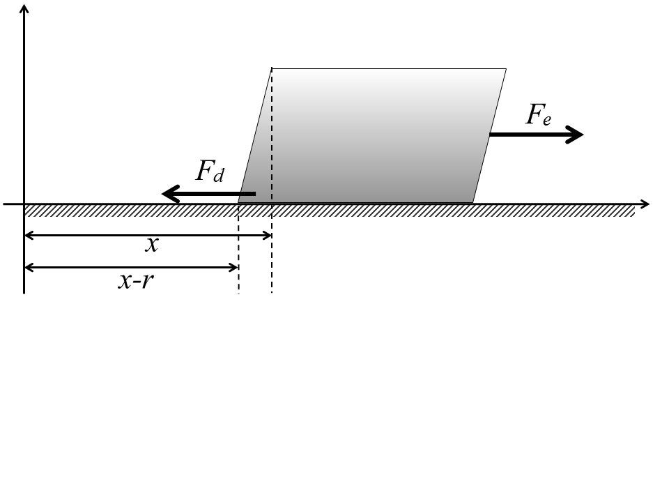
Moreover, the work of the external force changes the energy of the body, $E$. Therefore

(9) $$\dot{E}=F_{e}\dot{x}.$$

In this case thermodynamics requires that the damping force contributes only to the internal energy of the body. It is assumed that the external force accelerates the body and also that the body is deformable. In this homogeneous model, the deformation is expressed by the recoverable displacement, $r$. Therefore the kinetic and and elastic energies of the body are distinguished. This particular interpretation from [11] is not necessary, $r$ may denote a general internal variable.

The internal energy, $U$, is the difference of the total energy, $E$, the kinetic energy and a quadratic contribution of the internal variable. This form follows from the condition of thermodynamic stability in the state space [12].

(10) $$U=E-m\frac{{\dot{x}}^{2}}{2}-k\frac{r^{2}}{2},$$

where $k$ is a parameter like in elasticity. One assumes a particular kinematic condition in order to introduce an interpretation of $r$. When the instantaneous position of the body is the sum of a permanent and a recoverable displacements then a convenient method of their distinction is an additive separation of the displacement rates:

(11) $$V=\dot{x}=\dot{r}+z,$$

where $V$ is the rate of the position $x$, and $z$ is the rate of the permanent displacement. This rate type kinematical condition is convenient when distinguishing permanent and recoverable changes. (11) is analogous to the condition used in plasticity for the distinction of plastic and elastic strains (see e.g., [13, 14]). However, in friction the internal variable is not necessarily identical to the recoverable strain.

The dissipation can be calculated by the entropy balance, assuming that the entropy is the function of the internal energy only:

(12) $$\dot{S}(U)=\frac{1}{T}\left(F_{e}\dot{x}-mV\dot{V}-kr\dot{r}\right)\geq 0\,\ \Rightarrow\,T\dot{S}=F_{d}V-kr\dot{r}\geq 0.$$

The damping force and also the rate of the internal variable $\dot{r}$ are the constitutive quantities to be determined in accordance with the requirement of nonnegative entropy production. We connect the first term to friction interaction and the second term to frictional healing. In the vicinity of thermodynamic equilibrium, where both forces and fluxes are zero, the usual linear relationship is a consequence of Lagrange’s mean value theorem [15, 16]. $V$ and $r$ are thermodynamic state variables, therefore they can be considered as thermodynamic forces, while $\mu$ and $\kappa\dot{r}$ are to be determined constitutively, they are thermodynamic fluxes. The standard linear approximation results in equations that reflect well the thermodynamic admissibility of both velocity weakening and strengthening, however, did not incorporate the observed direct effect (logarithmic relaxation) [11].

However, in velocity-step experiments dynamic friction is a steady state phenomenon, we are looking for a deviation of the frictional coefficient from a fixed value, $\mu_{0}$, at a given $V_{0}$ reference velocity. On the other hand the internal variable is expected to be zero, when its time derivative is zero, in thermodynamic equilibrium. Therefore we face to a mixed, partial steady state, partial equilibrium situation. However, the dissipation inequality (12) may not characterize the deviation from steady state. What we need is an estimation of the deviation of the entropy production.

In our framework the steady state means a constant displacement rate, denoted by $V_{0}$. Therefore the internal energy should be determined accordingly

(13) $$U=E_{0}-m\frac{(V-V_{0})^{2}}{2}-k\frac{r^{2}}{2},$$

where $E_{0}$ is the energy of the body moving with the veolcity $V_{0}$. Then the calculation of the entropy production results in

(14) $$T\dot{S}(U)=F_{e}V-m(V-V_{0})\dot{V}-kr\dot{r}=F_{e}V_{0}+F_{d}(V-V_{0})-kr\dot{r}\geq 0.$$

We can introduce a friction specific entropy production with Amonton’s law:

(15) $$\frac{T}{F_{n}A}\dot{S}=\Sigma=\mu_{0}V_{0}+\Delta\mu(V-V_{0})-\kappa r\dot{r}\geq 0,$$

where $\mu_{0}=F_{e}/(AF_{n})$ is the external shear stress divided by the normal force, $\Delta\mu=F_{d}/(AF_{n})$ is the frictional stress divided by the normal force and $\kappa=\frac{k}{AF_{n}}$.

Now, it is straightforward to introduce a linear approximation for the increment of entropy production, as for the near equilibrium situation. However, in the following we apply a different starting point. Our fundamental assumption is that the leading term of the deviation from the steady state is logarithmic, while it is linear around equilibrium. We can formulate this hypothesis analogously to the classical exploitation of the entropy principle introducing the concept of incremental entropy production. We require that it is minimal at the steady state

(16) $$\Delta\Sigma=\Sigma-\Sigma_{steady}=\Sigma-\mu_{0}V_{0}=\Delta\mu\ln\left(\frac{V}{V_{0}}\right)-\kappa r\dot{r}\geq 0$$

We will call this hypothesis the principle of minimal incremental entropy production.

The required minimality ensures the asymptotic stability of the steady state if the evolution equations are constructed accordingly. In this respect the principle is similar to the role of the second law near to the equilibrium. On the other hand this hypothesis is a modification of the requirement of nonnegative excess entropy production of Glansdorff and Prigogine [18]. The difference of the Prigogine-Glansdorff requirement is the logarithmic deviation instead of a linear one. (The possibility of partial steady state, a specific property of friction, is important, too). Along with them we want to emphasize that the inequality here is not a law of nature, it is regarded as a convenient stability assumption [19, 20].

An example of similar logarithmic deviation is the thermodynamics of chemical kinetics, where the entropy production is a product of the chemical affinity and the reaction rate, but the Guldberg-Waage kinetic equations introduce an exponential relation [21]. It is remarkable that chemical equilibrium is considered as a steady state from a thermodynamic point of view, when forward and backward reactions are properly distinguished [22, 23]. Our formula corresponds a simple monomolecular reaction, which is actually equivalent to a single internal degree of freedom [21]. In friction the logarithmic deviation may be further motivated according to this chemical analogy [10].

Finally we remark, that the logarithmic form can be directly derived assuming that the internal energy is modified by a logarithmic velocity dependent term instead of a quadratic one $U=E_{0}-mV(Log(V/V_{0})-1)$.

(16) is similar to the usual entropy production in many respect. First of all the two terms are zero in the reference steady state and we assume that $\Delta\mu$ is a constitutive function of the logarithmic deviation, a function of the thermodynamic state variable. Therefore, in case of smooth functions the Lagrange mean value theorem ensures a linear homogeneous relationship between these constitutive quantities and the related thermodynamic forces also in this mixed steady-state equilibrium case.

The linearization of (16) result in the following expression:

(17) $$\Delta\mu =l_{1}\ln\left(\frac{V}{V_{0}}\right)-l_{12}\kappa r,$$

(18) $$\dot{r} =l_{21}\ln\left(\frac{V}{V_{0}}\right)-l_{2}\kappa r.$$

We will call (17)-(18) as thermodynamical aging law. (17) is identical to the Nakatani form of the constitutive law (5) and (18) is similar to (7).

The coefficient matrix may depend on the thermodynamic forces, in particular $l_{1}$, $l_{2}$, $l_{12}$ and $l_{21}$ may depend on the state variables $V$ and $r$ [24]. In the following we assume a strict linear relationship, when the coefficient matrix is constant. It is remarkable, that there are no reasons to assume symmetry or antisymmetry of the matrix. The conditions of Onsagerian statistical background cannot be introduced without a particular interpretation of the internal variable (more detailed arguments are given in [25, 26].

3. Different mechanisms of different relaxations

According to the experimental observations in case of velocity step and healing experiments, sometimes the internal variable changes when the surfaces slip, and sometimes its evolution is seemingly independent of the relative motion of the surfaces. This distinction is connected to the detailed mechanism of friction, and requires an extension of the modeling framework. In the following we will investigate the question of slip related internal variable evolution.

Ruina [6] applied this assumption directly to the relaxation. In our case that requires the modification of (18), assuming that the slip is what makes change of the internal variable and the rate of the variable is a consequence. In this case the time derivative in (18) is substituted by the space derivative and the rate is obtained as a consequence:

(19) $$\frac{dr}{dt}\rightarrow\frac{dr}{dx}=\frac{\dot{r}}{V}.$$

Performing this substitution in (18) leads to

(20) $$\dot{r}=l_{21}V\ln\left(\frac{V}{V_{0}}\right)-Vl_{2}\kappa r.$$

This equation, together with (17) will be called thermodynamical slip law. One can see, that the Nakatani transformed Ruina-law (5), (7) can be obtained if $l_{1}=a$, $l_{12}=-1/\kappa$, $l_{21}=-b/L$ and $l_{2}=1/(\kappa L)$. The number of phenomenological parameters is increased by one, from three to four, compared to the original Ruina theory. It is because $\kappa$ appears only as a multiplier of the cross coefficients $l_{12}$ and $l_{21}$. The slip governed modification represents a particular quasilinear form of the strictly linear relations of the thermodynamic aging law (17)-(18).

The slip condition of Ruina, expressed by (19) assumes that $V$ is the relative surface velocity, related to the permanent part of the displacement. When introducing a distinction between a permanent and a recoverable parts of the apparent displacement beyond the difference of the load point an relative surface velocities, one may expect, that only the permanent part contributes to the entropy production, to the evolution of the internal variable. For example an interpretation of the internal variable as recoverable displacement with the condition (11) leads to the following permanent displacement:

$$x_{per}=\int_{t_{0}}^{t}z(s)ds=x-r$$

Particular mechanisms require that the internal variable influences the slip. For example when the internal variable is connected to deformation of surface irregularities, then this conclusion is straightforward. Therefore we assume in general, that the internal variable directly influences the displacement and the reduced part is what influences the (incremental) entropy production. Hence we introduce $x_{red}=x-\alpha r$, where $0\leq\alpha\leq 1$ is the factor of slip reduction. If $\alpha=1$, then the internal variable can be interpreted as the recoverable part of the displacement [11].

Therefore the evolution equation of the internal variable is obtained by substituting the time derivative with the slip related change of the internal variable, as follows:

$$\frac{dr}{dt}\rightarrow\frac{dr}{d(x-\alpha r)}=\frac{\dot{r}}{V-\alpha\dot{r}}.$$

For the sake of simplicity $\alpha$ is constant. Then a simple rearrangement leads to the following evolution equation of the internal variable:

(22) $$\dot{r} =V\frac{l_{21}\ln\left(\frac{V}{V_{0}}\right)-l_{2}\kappa r}{1+\alpha\left(l_{21}\ln(\frac{V}{V_{0}})-l_{2}\kappa r\right)}.$$

Together with (17) we will call this equation thermodynamical friction law. This is an other particular quasilinear form of the thermodynamic aging law (17)-(18).

In the above thermodynamical models there is a direct effect and the conventional step test parameters are $a=l_{1}$ and $b=\frac{l_{12}l_{21}}{l_{2}}$. In the following we compare the performance of the obtained thermodynamic models with the classical models and experiments.

4. Velocity step tests

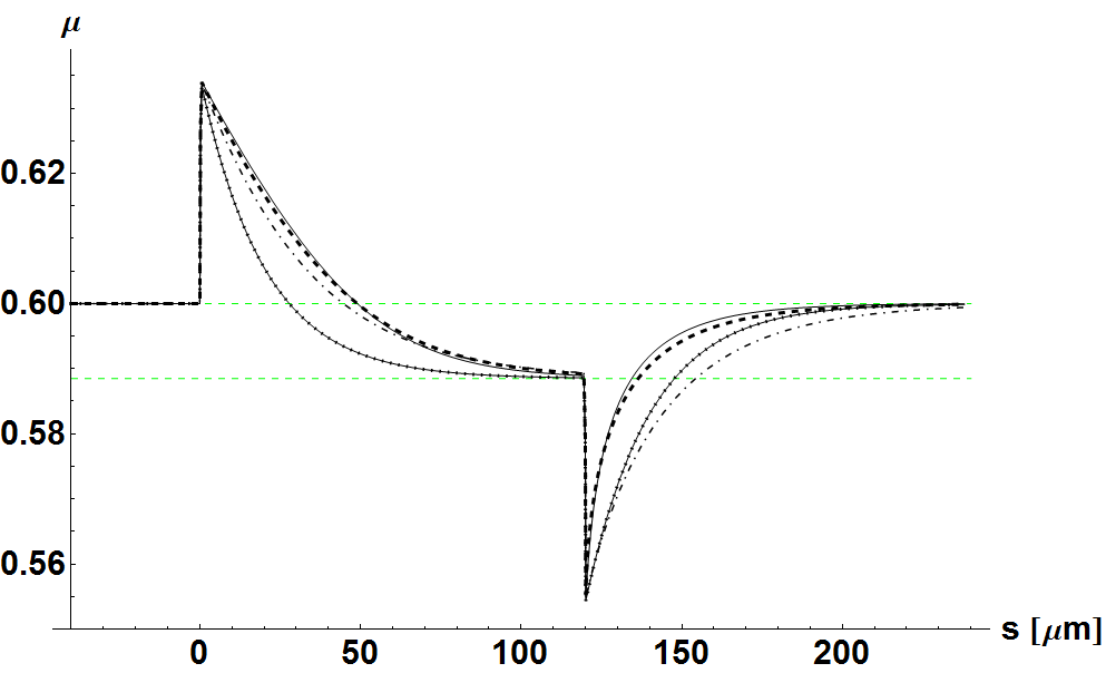
A comparison of the different rate- and state dependent friction laws is shown in Figure 2. The velocity weakening experiment is modeled with the following parameters:

$\mu_{0}=0.6$, $V_{0}=1\mu m/s$, $V_{1}=10\mu m/s$, $L=20\mu m$, $a=0.015$, and $b=0.02$.

Dieterich and Ruina models shown by a solid thin lines. The parameters of the thermodynamic friction model are calibrated to give the proper step conditions and relaxation speed: $l_{1}=a$, $l_{2}=1/L$, $l_{12}=b$, $l_{21}=l_{2}$. There are two additional parameters, the static recovery strength $\kappa$, analogous to a spring constant, and the factor of slip reduction $\alpha$. The dotted curve runs exactly over the line obtained by the Ruina model, because thermodynamic slip model recovers the Ruina case when $\kappa=1$ and $\alpha=0$. One obtains highly asymmetric relaxation curves choosing higher values of the slip reduction parameter $\alpha$ and with a proper choice one calculates curves that run close are pretty close to the Dieterich model. E.g. the thick dashed curve was calculated with $\kappa=0.85$ and $\alpha=8$. Moreover, one can obtain symmetric relaxation curves close to either the down or up relaxation curves of the Dieterich model with an appropriate choice of the parameters. For example the thick dotdashed line was calculated using $\kappa=0.7$ and $\alpha=2$.

The thermodynamic aging law produces asymmetric curves, similar to the Dieterich law.

Figure 2. Simulation of a velocity step test with different friction laws. The Dieterich and Ruina laws are drawn by solid thin lines. The thermodynamic friction law leads to the dotted line with $\kappa=1$ and $\alpha=0$ parameters running over the line of Ruinalaw. The dashed line with parameters $\kappa=0.85$ and $\alpha=8$ runs close to the Dieterich law. For the dotdashed line the parameters are $\kappa=0.7$ and $\alpha=2$.

5. Healing

The interpretation of healing is contradictory, therefore we have chosen the experiments and strategy of Beeler an Tullis [27, 3] for demonstration. They performed healing experiments with different machine rigidity. One of them $k=0.002$ was the natural elasticity of the experimental device, in this case the load point velocity was $V_{0}=1\mu m/s$. With the $k=0.074$ servocontrolled value the load point velocity was $V_{0}=0.316\mu m/s$. In both cases the rock parameters were $L=3\mu m$, $a=0.009$, and $b=0.008$. The data points in the first and second cases are shown on figure 3 by circle and rectangles, respectively. The simulation used the experimental rock parameters of Beeler et al. [27] and the additional parameters were chosen as $\alpha=0.75$ and $\kappa=0.9$. Then we have obtained the dashed curve for the $k=0.074$ case and the dotted one for $k=0.002$.

Figure 3. Simulation of the healing experiments of Beeler et al [27]. The experimental data for the $k=0.002$ case is shown by the big circles and for the $k=0.074$ case by the rectangles. The dotted curve is calculated by the thermodynamic friction model for $k=0.002$. The $k=0.074$ parameter resulted in the dashed curve.

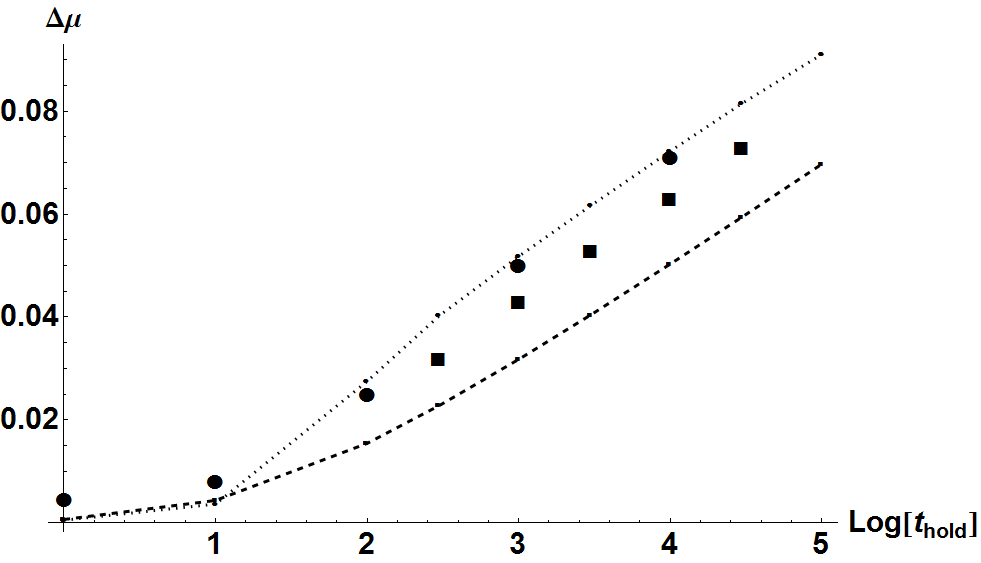
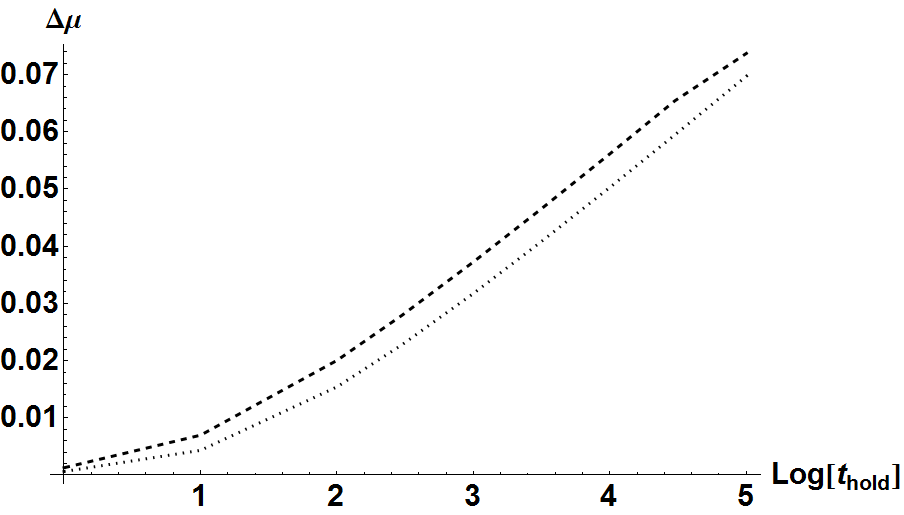
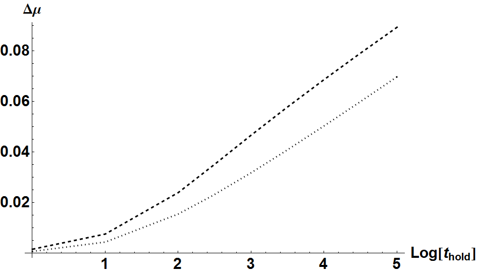
Figures 4 and 5 show the effect of changing the initial velocity and the machine rigidity. In figure 4 the simulation of the healing experiment with the more rigid machine is shown, where the parameter values are $k=0.002$, $V_{0}=1\mu m/s$, $L=3\mu m$, $a=0.009$, $b=0.008$, $\alpha=0.75$ and $\kappa=0.9$ (dotted curve in figure 3). Increasing the velocity to $V_{0}=2\mu m/s$ pushes the curve upward and parallel to the original one, shown with the dashed curve. In figure 5 the effect of softening is demonstrated, the dashed curve is calculated with $k=0.02$. The dotted curve is identical to the one in figure 4. The increase of the healing effect qualitatively corresponds to the experimental observations.

Figure 4. The effect of larger steade state velocity for healing. $V_{0}=1\mu m/s$, dotted curve, $V_{0}=2\mu m/s$, dashed one.

Figure 5. The effect of softened machine for healing. $k=0.002$, dotted curve, $k=0.02$, dashed one.

6. Summary and conclusion

A non-equilibrium thermodynamic model with a single internal variable of rate- and state-dependent friction was proposed. The model introduced the following basic assumptions:

• The deviation from the steady state is logarithmic.

• The change of internal variable is due to a reduced slip, and the reduction is proportional to the value of the internal variable.

The obtained thermodynamic friction model generalizes the well known Dieterich and Ruina laws with two additional parameters.

• For velocity step tests it interpolates between the Dieterich and Ruina laws. The form of the relaxation depends on the additional parameters. One can obtain symmetric up and down relaxation curves that are either close to the curves of Ruina relaxation or are close to the Dieterich type relaxation, but with less apparent linear part.

• Simulations show promising results for healing experiments, both quantitavely and qualitatively.

7. Acknowledgement

The work was supported by the grants Otka K81161 and K104260.

References

- [1] J. H. Dieterich. Time-dependent friction in rocks. Journal of Geophysical Research, 77(20):3690–3697, 1972.
- [2] J. H. Dieterich. Time-dependent friction and the mechanics of stick-slip. Pure and Applied Geophysics, 116(4-5):790–806, 1978.
- [3] C. Marone. Laboratory-derived friction laws and their application to seismic faulting. Annual Rev. Earth Planet. Sci., 26:643–696, 1998.
- [4] C. Marone, C. B. Raleigh, and C. H. Scholz. Frictional behavior and constitutive modeling of simulated fault gouge. Journal of Geophysical Research, 95(B5):7007–7025, 1990.
- [5] J. H. Dieterich. Modeling of rock friction 1. experimental results and constitutive equations. Journal of Geophysical Research, 84(B5):2161–2168, 1979.
- [6] A. Ruina. Slip instability and state variable friction laws. Journal of Geophysical Research, 88:10359–10370, 1983.
- [7] K. Nagata, M. Nakatani, and S. Yoshida. A revised rate- and state-dependent friction law obtained by constraining constitutive and evolution laws separately with laboratory data. Journal of Geophysical Research, 117:B02314, 2012.
- [8] G. Perrin, J. R. Rice, and Zheng G. Self-healing slip pulse on a frictional surface. Journal of Mechanics and Physics of Solids, 43:1461–1495, 1995.
- [9] N. Kato and T. E. Tullis. A composite rate- and state-dependent law for rock friction. Geophysical Research Letters, 28(6):1103–1106, 2001.
- [10] M. Nakatani. Conceptual and physical clarification of rate and state friction: Frictional sliding as a thermally activated rheology. Journal of Geophysical Research, 106(B7):13347–13380, 2001.
- [11] N. Mitsui and P. Ván. Thermodynamic aspects of rock friction. Acta Geodaetica et Geophysica, 49:135–146, 2014. arXiv:1312.4930 [physics.geo-ph].
- [12] J. Verhás. Thermodynamics and Rheology. Akadémiai Kiadó and Kluwer Academic Publisher, Budapest, 1997.
- [13] T. Fülöp and P. Ván. Kinematic quantities of finite elastic and plastic deformations. Mathematical Methods in the Applied Sciences, 35:1825–1841, 2012. arXiv:1007.2892v1.
- [14] A. Rusinko and K. Rusinko. Plasticity and Creep of Metals. Springer, 2011.
- [15] M. G. Gurtin. Generalized Ginzburg-Landau and Cahn-Hilliard equations based on a microforce balance. Physica D, 92:178–192, 1996.
- [16] P. Ván. Weakly nonlocal irreversible thermodynamics. Annalen der Physik (Leipzig), 12(3):146–173, 2003. (cond-mat/0112214).
- [17] P. Ván. Abszolút folyadékmechanika. volume 18 of Mérnökgeológia-Kőzetmechanika Kiskönyvtár, page ?, Budapest, 2015. Hantken Kiadó. in Hungarian.
- [18] P. Glansdorff and I. Prigogine. Thermodynamic Theory of Structure, Stability and Fluctuations. Wiley-Interscience, London-etc., 1971.
- [19] J. Keizer and R. F. Fox. Qualms regarding the range of validity of the Glansdorff-Prigogine criterion for stability of non-equilibrium states. Proceedings of the National Academy of Sciences, USA, 71(1):192–196, 1974.
- [20] P. Glansdorff, G. Nicolis, and I. Prigogine. The thermodynamic stability theory of nonequilibrium steady-states. Proceedings of the National Academy of Sciences, USA, 71(1):197–199, 1974.
- [21] S. R. de Groot and P. Mazur. Non-equilibrium Thermodynamics. North-Holland Publishing Company, Amsterdam, 1962.
- [22] S. Lengyel and I. Gyarmati. On the thermodynamics of elementary chemical reactions in homogeneous systems. The Journal of Chemical Physics, 75(5):2384–2389, 1981.
- [23] S. Lengyel. Chemical kinetics and thermodynamics (a history of their relationship). Computers Math. Applic., 17(1-3):443–455, 1989.
- [24] I. Gyarmati. The wave approach of thermodynamics and some problems of non-linear theories. Journal of Non-Equilibrium Thermodynamics, 2:233–260, 1977.
- [25] P. Ván, A. Berezovski, and J. Engelbrecht. Internal variables and dynamic degrees of freedom. Journal of Non-Equilibrium Thermodynamics, 33(3):235–254, 2008. cond-mat/0612491.
- [26] P. Ván, C. Papenfuss, and A. Berezovski. Thermodynamic approach to generalized continua. Continuum Mechanics and Thermodynamics, 25(3):403–420, 2014. Erratum: 421-422, arXiv:1304.4977.
- [27] N. M. Beeler, T. E. Tullis, and J. D. Weeks. The roles of time and displacement in the evolution effect in rock friction. Geophysical Research Letters, 21(18):1987–1990, 1994.