Condition Metrics in the Three Classical Spaces

Abstract.

Let $(\mathcal{M},g)$ be a Riemannian manifold and $\mathcal{N}$ a $\mathcal{C}^{2}$ submanifold without boundary. If we multiply the metric $g$ by the inverse of the squared distance to $\mathcal{N}$, we obtain a new metric structure on $\mathcal{M}\setminus\mathcal{N}$ called the condition metric. A question about the behaviour of the geodesics in this new metric arises from the works of Shub and Beltrán: is it true that for every geodesic segment in the condition metric its closest point to $\mathcal{N}$ is one of its endpoints? Previous works show that the answer to this question is positive (under some smoothness hypotheses) when $\mathcal{M}$ is the Euclidean space $\mathbb{R}^{n}$. Here we prove that the answer is also positive for $\mathcal{M}$ being the sphere $\mathbb{S}^{n}$ and we give a counterexample showing that this property does not hold when $\mathcal{M}$ is the hyperbolic space $\mathbb{H}^{n}$.

1. Introduction

In this paper we study the following problem: let $(\mathcal{M},g)$ be a Riemannian manifold and $\mathcal{N}$ a $\mathcal{C}^{2}$ submanifold without boundary. We consider a new metric structure $g_{\kappa}$ on $\mathcal{M}\setminus\mathcal{N}$ obtained by multiplying the metric $g$ by the inverse of the squared distance to $\mathcal{N}$. This is, for a point $x\in\mathcal{M}\setminus\mathcal{N}$,

$$g_{x,\kappa}=d(x,\mathcal{N})^{-2}g_{x},$$

where $d(x,\mathcal{N})$ is the Riemannian distance (w.r.t. $g$) from $x$ to $\mathcal{N}$. We call $g_{\kappa}$ the condition metric on $\mathcal{M}\setminus\mathcal{N}$. The interest of the condition metric comes from the papers of Shub [8] and Beltrán-Shub [3], where they improve complexity bounds for solving systems of polynomial equations in terms of a certain condition metric on the space $\mathcal{M}$ of systems, with $\mathcal{N}$ being the set of ill-conditioned systems to avoid. Although $(\mathcal{M}\setminus\mathcal{N},g_{\kappa})$ is not always a Riemannian manifold, there is still a sensible way to define the concept of geodesic as a path that locally minimizes the distance. Geodesics in the condition metric try to avoid the submanifold $\mathcal{N}$ because being close to $\mathcal{N}$ increases their length. An interesting question about these geodesics is the following: given a geodesic segment in the condition metric, is it true that the closest point from the segment to $\mathcal{N}$ is one of its endpoints? Sometimes we will refer to this property as ‘the worst is at the endpoints’.

The function $d(\cdot,\mathcal{N})$ is not always smooth, but it can be shown that it is always Lipschitz ([1, Proposition 9]). In this context the condition metric defines a Lipschitz-Riemann structure (in the sense of [1, Definition 2]) and we have to consider Lipschitz curves on $\mathcal{M}\setminus\mathcal{N}$. For such a curve $\gamma:I\rightarrow\mathcal{M}\setminus\mathcal{N}$ the Rademacher Theorem states that the tangent vector $\dot{\gamma}$ exists almost everywhere, so it makes sense to define the arc length of $\gamma$ w.r.t. $g_{\kappa}$ by

$$L_{\kappa}(\gamma)=\int_{I}\|\dot{\gamma}(t)\|_{\kappa}dt=\int_{I}\|\dot{\gamma}(t)\|d(\gamma(t),\mathcal{N})^{-1}dt.$$

With this definition of arc length, we say that a path $\gamma:[a,b]\rightarrow\mathcal{M}\setminus\mathcal{N}$, parametrized by arc length, is a minimizing geodesic in the condition metric if $L_{\kappa}(\gamma)\leq L_{\kappa}(c)$ for any Lipschitz curve $c:[a,b]\rightarrow\mathcal{M}\setminus\mathcal{N}$ with $\gamma(a)=c(a)$ and $\gamma(b)=c(b)$. We say that $\gamma$ is a geodesic if it is locally a minimizing geodesic.

A sufficient condition for a geodesic $\gamma$ in the condition metric to satisfy that ‘the worst is at the endpoints’ is that the function

(1.1) $$t\mapsto\frac{1}{d(\gamma(t),\mathcal{N})}$$

is convex (recall that a function $f:(a,b)\rightarrow\mathbb{R}$ is convex if for every $x,y\in(a,b)$ and for every $t\in[0,1]$, $f((1-t)x+ty)\leq(1-t)f(x)+tf(y)$). If we examinate some examples in detail, we rapidly realize that a stronger property is satisfied in many cases: the logarithm of the function (1.1) is also a convex function (this means that (1.1) is a log-convex function). We wonder if this is true in general. More precisely, is the real function

(1.2) $$t\mapsto\log\frac{1}{d(\gamma(t),\mathcal{N})}$$

convex for every geodesic $\gamma$ in the condition metric? Answering this question is the main goal of our work and our results about it are summarized in theorems 1.2 and 1.3. If (1.2) is a convex function for every geodesic $\gamma$ in $g_{\kappa}$, we will say that the self-convexity property is satisfied (maybe the term self-log-convexity would be more accurate, but we prefer to use this shorter term). If the distance function $d(\cdot,\mathcal{N})$ is smooth, then the self-convexity property is equivalent to

(1.3) $$\frac{d^{2}}{dt^{2}}\log\frac{1}{d(\gamma(t),\mathcal{N})}\geq 0\quad\equiv\quad\frac{d^{2}}{dt^{2}}\log d(\gamma(t),\mathcal{N})\leq 0,$$

but if it is not, deciding whether (1.2) is a convex function or not is much harder a problem. In many cases we will restrict ourselves to the largest open set $\mathcal{U}\subseteq\mathcal{M}\setminus\mathcal{N}$ such that for every $x\in\mathcal{U}$ the function $d(\cdot,\mathcal{N})$ is smooth and there is a unique closest point to $x$ in $\mathcal{N}$. If (1.2) is a convex function for every geodesic contained in $\mathcal{U}$, we will say that the smooth self-convexity property is satisfied. The following result solves the problem for the case $\mathcal{M}=\mathbb{R}^{n}$:

Theorem 1.1.

[1, Theorem 2] The smooth self-convexity property is satisfied for the Euclidean space $\mathcal{M}=\mathbb{R}^{n}$ endowed with the usual inner product $\langle\cdot,\cdot\rangle$, and $\mathcal{N}$ a complete $\mathcal{C}^{2}$ submanifold without boundary.

Our first result is

Theorem 1.2.

The smooth self-convexity property is satisfied for the sphere $\mathcal{M}=\mathbb{S}^{n}$ and $\mathcal{N}$ a complete $\mathcal{C}^{2}$ submanifold without boundary.

Let us now briefly discuss the importance of Theorem 1.2 in the context of the question that originated the study of condition metrics. In [8, 3] the authors noted that studying the condition metric in the set

$$\mathcal{M}_{poly}=\{(f,\zeta)\ |\ f\text{ a polynomial system},\zeta\in\mathbb{P}(\mathbb{C}^{n+1}),f(\zeta)=0\},$$

where polynomial systems are assumed to be homogeneous of fixed degree in $n+1$ complex variables, with

$$\mathcal{N}_{poly}=\{(f,\zeta)\in\mathcal{M}\ |\ \zeta\text{ is a degenerate zero of }f\},$$

could be useful for the design of fast homotopy methods to solve polynomial systems (indeed, the metric used in [3] is not exactly the condition metric, but it is closely related to it from [4, Corollary 6]). The question of self-convexity turned out to be extremely difficult to analyze in this context, which motivated a theoretical and numerical study [1, 2, 5] of the linear case

$$\mathcal{M}_{lin}=\{(M,\zeta)\in\mathbb{C}^{n\times(n+1)}\times\mathbb{P}(\mathbb{C}^{n+1})\ |\ M\zeta=0\},$$

(we denote by $\mathbb{C}^{n\times(n+1)}$ the set of $n\times(n+1)$ complex matrices) with

$$\mathcal{N}_{lin}=\{(M,\zeta)\in\mathcal{M}\ |\ \dim\ker M>1\}.$$

Using quite sophisticated an argument, it was proved in [2] that the self-convexity property holds in $(\mathcal{M}_{lin},\mathcal{N}_{lin})$. The argument considers a stratification of the set $\mathbb{C}^{n\times(n+1)}$ of complex matrices based on the singular value descomposition. For each $u$-uple $(k)=(k_{1},...,k_{u})$ of integers with $k_{1}+\cdots+k_{u}=n$, consider the set $\mathcal{P}_{(k)}$ of matrices whose $k_{1}$ first singular values are equal, whose $k_{2}$ following singular values are equal, etcetera. That is,

$$\mathcal{P}_{(k)}=\{M\in\mathbb{C}^{n\times(n+1)}\ |\ \text{svd}(M)=(\underbrace{\sigma_{1},...,\sigma_{1}}_{k_{1}},\underbrace{\sigma_{2},...,\sigma_{2}}_{k_{2}},...,\underbrace{\sigma_{u},...,\sigma_{u}}_{k_{u}})\},$$

with $\sigma_{1}>\sigma_{2}>\cdots>\sigma_{u}>0$. Also let

$$\mathcal{N}_{(k)}=\{M\in\mathbb{C}^{n\times(n+1)}\ |\ \text{svd}(M)=(\underbrace{\sigma_{1},...,\sigma_{1}}_{k_{1}},\underbrace{\sigma_{2},...,\sigma_{2}}_{k_{2}},...,\underbrace{\sigma_{u-1},...,\sigma_{u-1}}_{k_{u-1}},\underbrace{0,...,0}_{k_{u}})\}.$$

These sets will play the role of $\mathcal{M}$ and $\mathcal{N}$. It can be shown that $\mathcal{P}_{(k)}$ is a smooth manifold [2, Proposition 16]. Although in this case $\mathcal{N}_{(k)}$ is not contained in $\mathcal{P}_{(k)}$, $\mathcal{N}_{(k)}$ lies in the boundary of $\mathcal{P}_{(k)}$, so the condition metric in $(\mathcal{P}_{(k)},\mathcal{N}_{(k)})$ can be defined. The distance function is smooth in $\mathcal{P}_{(k)}\setminus\mathcal{N}_{(k)}$ and, surprisingly, the smooth self-convexity property (thus the self-convexity property) holds for each pair $(\mathcal{P}_{(k)},\mathcal{N}_{(k)})$. Then the authors glue all the pieces together and lift the result up to $(\mathcal{M}_{lin},\mathcal{N}_{lin})$, thus proving that the smooth self-convexity property is satisfied in the linear case.

The problem about self-convexity in $(\mathcal{M}_{poly},\mathcal{N}_{poly})$ remains open, but in view of the fact that self-convexity holds for such complicated cases as ($\mathcal{P}_{(k)},\mathcal{N}_{(k)})$, $(\mathcal{M}_{lin},\mathcal{N}_{lin})$ and $\mathbb{R}^{n}$ together with any $\mathcal{C}^{2}$ submanifold (Theorem 1.1), one could hope for the existence of a general argument proving that the smooth self-convexity property holds for every pair $(\mathcal{M},\mathcal{N})$ under very general assumptions, opening the path to a solution for $(\mathcal{M}_{poly},\mathcal{N}_{poly})$. Theorem 1.2 adds another collection of cases to this list, with $\mathcal{M}$ being $\mathbb{S}^{n}$ and $\mathcal{N}$ any $\mathcal{C}^{2}$ submanifold.

Despite all this (somehow empirical) evidence, our last theorem shows that smooth self-convexity can fail, even in a very familiar space.

Theorem 1.3.

If the ambient manifold is the hyperbolic space $\mathcal{M}=\mathbb{H}^{n}$ and $\mathcal{N}$ is a single point, then for every geodesic $\gamma$ in the condition metric the function $t\mapsto\log\left(\frac{1}{d(\gamma(t),\mathcal{N})}\right)$ is concave. Moreover, if $\gamma^{\prime}(t)$ does not point towards the point $\mathcal{N}$, then the function is strictly concave at $t$. Thus in this case the self-convexity property is not satisfied.

This result, together with the cases of $\mathbb{R}^{n}$ (Theorem 1.1) and $\mathbb{S}^{n}$ (Theorem 1.2), completes the study of the smooth self-convexity property in the three classical spaces.

2. Some examples

In this section we will present some examples of condition metrics varying $\mathcal{M}$ and $\mathcal{N}$. From now on, we will denote $d(x,\mathcal{N})$ simply by $\rho(x)$.

Example 2.1.

If we take $\mathcal{M}=\mathbb{R}^{2}$ the Euclidean plane and $\mathcal{N}$ the line $\{y=0\}$, then de distance from a point $(x,y)$ to $\mathcal{N}$ is $\rho(x,y)=y$ and the condition metric reads $g_{(x,y),\kappa}=\frac{1}{y^{2}}\langle\cdot,\cdot\rangle$. In this case we obtain two copies of the Poincaré half space and the function (1.2) is convex for every geodesic segment, supporting Theorem 1.1.

Example 2.2.

Let $\mathcal{M}$ be $\mathbb{R}^{2}$ as in the previous example and let $\mathcal{N}$ be a single point. For example, let $\mathcal{N}$ be the origin $\mathcal{N}=\{(0,0)\}$ as in Figure 1.

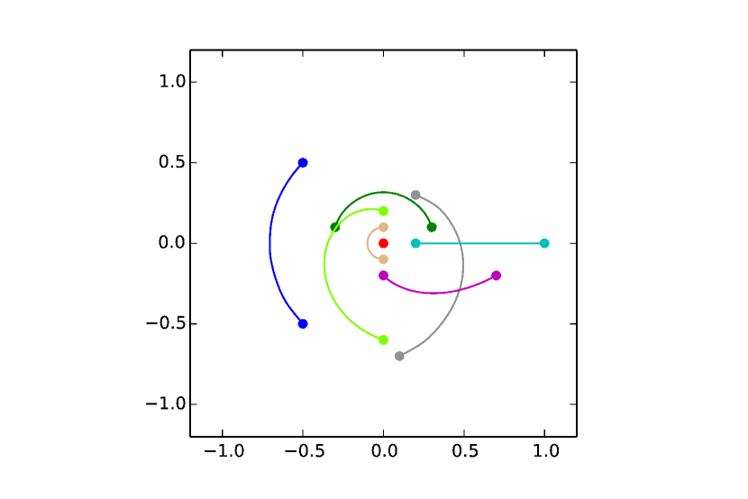
(a) Geodesic segments.

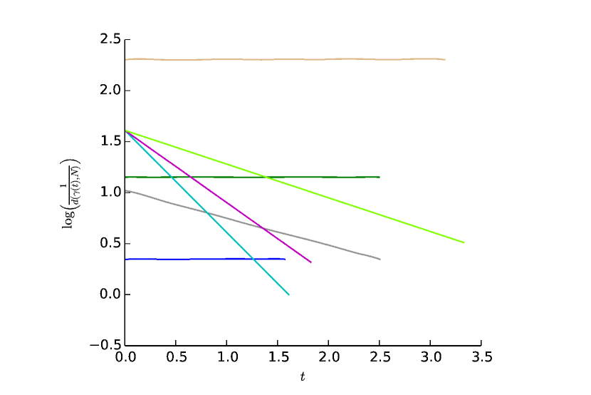
(b) Corresponding (1.2) functions.

Figure 1. Some geodesic segments in the condition metric when $\mathcal{M}$ is the Euclidean plane $\mathbb{R}^{2}$ and $\mathcal{N}$ is the red point, $(0,0)$. In this case (1.2) functions are affine functions, thus convex.

The condition metric is given by $g_{(x,y),\kappa}=\frac{1}{\|(x,y)\|^{2}}\langle\cdot,\cdot\rangle$. In this case we are on the hypotheses of Theorem 1.1, so the function (1.2) is convex on $\mathcal{M}\setminus\mathcal{N}$. Moreover it can be shown that $(\mathbb{R}^{2}\setminus\{(0,0)\},g_{\kappa})$ is isometric to a cylinder via the isometry $f:\mathbb{R}^{2}\rightarrow\mathbb{R}^{3}$ given by

$$f(x,y)=\left(\frac{x}{\|(x,y)\|},\frac{y}{\|(x,y)\|},\log\|(x,y)\|\right).$$

Example 2.3.

If we take out two points from the plane, let us say we set $\mathcal{N}=\{(-1,0),(1,0)\}$, then $\rho(x)$ is a piecewise function smooth at every point $(x,y)$ with $x>0$ or $x<0$, but it is not smooth on the line $\{x=0\}$ and for every point in this line there are two closest points to $x$ in $\mathcal{N}$. Theorem 1.1 guarantees that (1.2) is a convex function for every geodesic segment contained in one of the two semiplanes $\{x>0\}$ or $\{x<0\}$, but it says nothing about those geodesic segments crossing the line $\{x=0\}$. Figure 2 shows a picture of the situation.

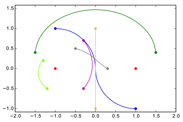
(a) Geodesic segments.

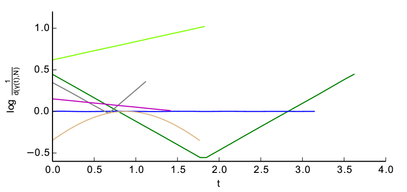
(b) Corresponding (1.2) functions.

Figure 2. Some geodesic segments in the condition metric when $\mathcal{M}=\mathbb{R}^{2}$ and $\mathcal{N}$ consists of the two red points.

As we can see, if a geodesic segment which crosses the line $\{x=0\}$ has only one point in this line, then its corresponding (1.2) function is convex because both branches of the function are convex and, when crossing the line, the distance function reaches a global maximum, hence (1.2) reaches a minimum and is convex (see Lemma 3.2). However, the function (1.2) corresponding to the light brown segment, which is entirely contained in the problematic line, is not convex.

The general case for $\mathcal{N}$ being a finite number of points in the plane is determined by the Voronoi diagram of the points. Inside the Voronoi cells (1.2) is convex by Theorem 1.1, but we cannot say much about what happens for segments crossing some edges and vertices.

Example 2.4.

If $\mathcal{M}$ is again the plane and $\mathcal{N}$ is a hyperbola, then the situation is very similar to the example above (see Figure 3). The function (1.2) is convex for every geodesic segment contained in the open set $\mathcal{U}$ where $\rho$ is smooth and there is a single closest point in the hyperbola, but it fails to be convex for the blue segment, which is entirely contained in the $y$ axis: if we have to move from one of the blue dots to the other one, we have to go through the neck of the hyperbola.

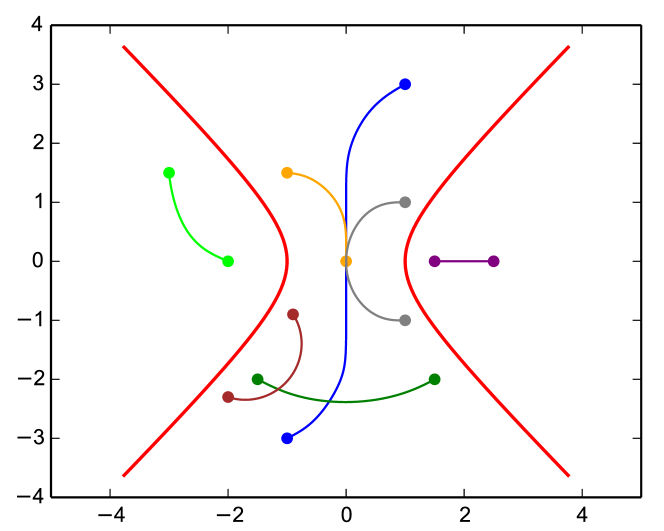
(a) Geodesic segments.

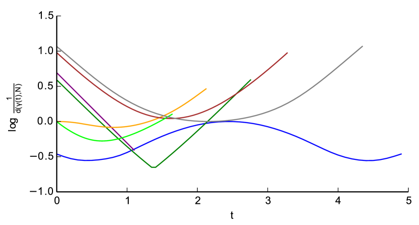
(b) Corresponding (1.2) functions.

Figure 3. Some geodesic segments in the condition metric when $\mathcal{M}$ is the Euclidean plane $\mathbb{R}^{2}$ and $\mathcal{N}$ is a hyperbola (in red). Self-convexity fails for the blue segment, which is not contained in $\mathcal{U}$.

Example 2.5.

Let us move from the Euclidean ambient manifold to the sphere. Let $\mathcal{M}=\mathbb{S}^{2}$ and $\mathcal{N}$ a single point. For example $\mathcal{N}=\{(0,0,1)\}$ be the north pole $N$, as in Figure 4. In spherical coordinates, the distance from a point $(\theta,\phi)$ to the north pole is simply $\rho(\theta,\phi)=\theta$, hence the local expression for the condition metric in this case is $g_{(\theta,\phi),\kappa}=\frac{1}{\theta^{2}}g_{(\theta,\phi)}$, where $g$ is the usual metric on the sphere in spherical coordinates. The function $\rho$, defined on $\mathbb{S}^{2}\setminus\{N\}$, is not smooth at the south pole $S=\{(0,0,-1)\}$, but it is smooth elsewhere, so our main result about self-convexity on the sphere says that (1.2) is convex for every geodesic segment contained in $\mathbb{S}^{2}\setminus\{N,S\}$. However, as a consequence of Lemma 3.2, in this particular case self-convexity also holds at the south pole.

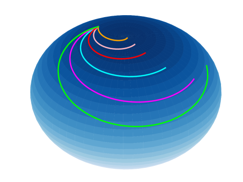
(a) Geodesic segments.

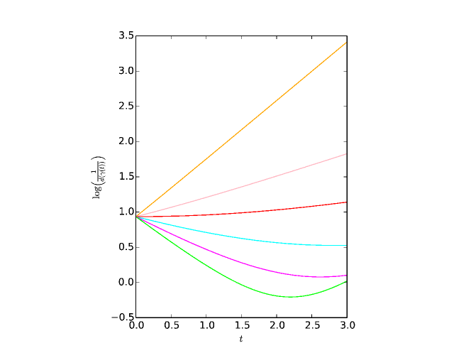
(b) Corresponding (1.2) functions.

Figure 4. Some geodesic segments in the condition metric when $\mathcal{M}=\mathbb{S}^{2}$ and $\mathcal{N}$ is a single point, the north pole.

Example 2.6.

If $\mathcal{M}$ is the paraboloid given by $z=x^{2}+y^{2}$ and $\mathcal{N}$ is the vertex $(0,0,0)$, then the distance from a point $(z\cos\phi,z\sin\phi,z^{2})$ to $\mathcal{N}$ is given by the formula $\frac{1}{4}\left(2z\sqrt{4z^{2}+1}+\arcsin 2z\right)$. In this case the function $\rho$ is smooth everywhere in $\mathcal{M}\setminus\mathcal{N}$ and the numerical experiments suggest that the self-convexity property also holds in this case. Geodesic segments exhibit a curious behaviour: if we throw a geodesic in a direction not opposed to the vertex, it will always eventually fall down towards the vertex describing a spiral (see Figure 5).

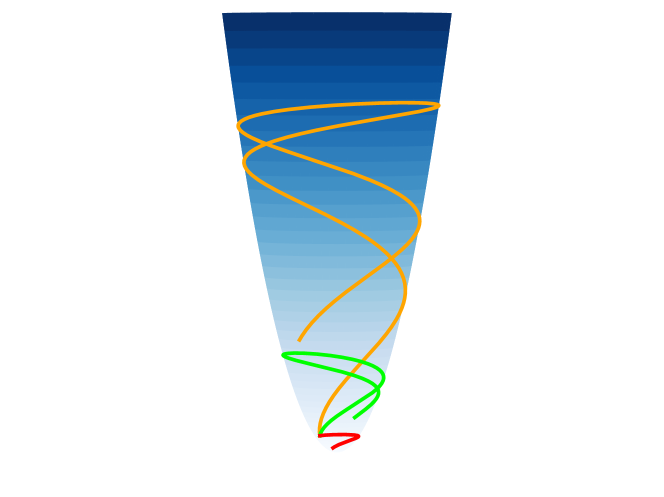
(a) Geodesic segments.

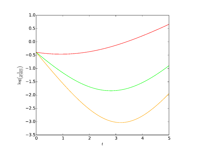
(b) Corresponding (1.2) functions.

Figure 5. Some geodesic segments in the condition metric when $\mathcal{M}$ is the paraboloid $z=x^{2}+y^{2}$ and $\mathcal{N}$ is the vertex of the paraboloid.

3. Punctured $\mathbb{S}^{n}$

Now let us study the case when $\mathcal{M}$ is the sphere $\mathbb{S}^{n}$ and $\mathcal{N}$ is a single point, the north pole $\mathcal{N}=\{(1,0,...,0)\}$. The sphere may be parametrized in spherical coordinates as

$$x_{1} =\cos\theta_{1},$$

$$x_{2} =\sin\theta_{1}\cos\theta_{2},$$

$$x_{3} =\sin\theta_{1}\sin\theta_{2}\cos\theta_{3},$$

$$\vdots$$

$$x_{n} =\sin\theta_{1}\cdots\sin\theta_{n-1}\cos\theta_{1},$$

$$x_{n+1} =\sin\theta_{1}\cdots\sin\theta_{n-1}\sin\theta_{n},$$

where $\theta_{1},...,\theta_{n-1}\in(0,\pi)$ and $\theta_{n}\in(-\pi,\pi)$. The metric tensor with this parametrization is the diagonal matrix

$$g_{\theta}=\sum_{i=1}^{n}\left(\prod_{j=1}^{i-1}\sin^{2}\theta_{j}\right)d\theta_{i}^{2}$$

and the distance from a point $\theta=(\theta_{1},...,\theta_{n})$ to the north pole is $\theta_{1}$. This yields the condition metric $g_{\theta,\kappa}=\theta_{1}^{-2}g_{\theta}$. After the computation of the Christoffel symbols (see, for example, [9]) $\Gamma_{ij}^{1}$, we obtain

$$\Gamma_{11}^{1}=-\frac{1}{\theta_{1}},\qquad\Gamma_{12}^{1}=0,\qquad\Gamma_{22}^{1}=-\frac{\theta_{1}\sin\theta_{1}\cos\theta_{1}-\sin^{2}\theta_{1}}{\theta_{1}},$$

and, for every $j>2$,

$$\Gamma_{1j}^{1}=0,\qquad\Gamma_{jj}^{1}=-\frac{\theta_{1}\sin\theta_{1}\cos\theta_{1}-\sin^{2}\theta_{1}}{\theta_{1}}\prod_{r=2}^{j-1}\sin^{2}\theta_{r}.$$

The remaining $\Gamma_{ij}^{1}$ are zero. With the Christoffel symbols we obtain the first of the geodesic equations, which is the only one that we will need.

$$\ddot{\theta}_{1}-\frac{1}{\theta_{1}}\dot{\theta}_{1}^{2}-\frac{\theta_{1}\sin\theta_{1}\cos\theta_{1}-\sin^{2}\theta_{1}}{\theta_{1}}\dot{\theta}_{2}^{2}$$

(3.1) $$-\sum_{j=3}^{n}\left(\frac{\theta_{1}\sin\theta_{1}\cos\theta_{1}-\sin^{2}\theta_{1}}{\theta_{1}}\prod_{r=2}^{j-1}\sin^{2}\theta_{r}\right)\dot{\theta}_{j}^{2} =0.$$

Proposition 3.1.

For $\mathcal{M}=\mathbb{S}^{n}$ and $\mathcal{N}$ a single point, the smooth self-convexity property holds.

Proof.

Let $\gamma$ be a geodesic, so the distance function from $\gamma$ to the north pole is $\gamma_{1}$. Replacing $\gamma$ in (3.1) and multiplying this equation by $\gamma_{1}$, we obtain

$$\gamma_{1}^{\prime\prime}\gamma_{1}-\gamma_{1}^{\prime 2} =(\gamma_{1}\sin\gamma_{1}\cos\gamma_{1}-\sin^{2}\gamma_{1})\gamma_{2}^{\prime 2}$$

(3.2) $$+\sum_{j=3}^{n}\left((\gamma_{1}\sin\gamma_{1}\cos\gamma_{1}-\sin^{2}\gamma_{1})\prod_{r=2}^{j-1}\sin^{2}\gamma_{r}\right)\gamma_{j}^{\prime 2}.$$

The real function $x\mapsto x\sin x\cos x-\sin^{2}x$ is negative for every $x\in(0,\pi)$, so the left hand side of (3.2) is always negative. Now note that

$$\frac{d^{2}}{dt^{2}}\log\rho(\gamma(t))=\frac{d^{2}}{dt^{2}}\log\gamma_{1}(t)=\frac{\gamma_{1}^{\prime\prime}\gamma_{1}-\gamma_{1}^{\prime 2}}{\gamma_{1}^{2}}\leq 0,$$

satisfying (1.3). ∎

Although it is not clear in spherical coordinates, the distance function is not smooth at the south pole $(-1,0,...,0)$, but the self-convexity property also holds here. In order to prove this fact, we will need the following result.

Lemma 3.2.

Let $f:(a,b)\rightarrow\mathbb{R}$ a continuous function that reaches a global minimum at $c\in(a,b)$. If both branches $f_{1}=f\big{|}_{(a,c)}$ and $f_{2}=f\big{|}_{(c,b)}$ are convex, then $f$ is convex.

The proof is left as an exercise to the reader.

Corollary 3.3.

For $\mathcal{M}=\mathbb{S}^{n}$ and $\mathcal{N}$ a single point, the self-convexity property holds.

Proof.

Proposition 3.1 guarantees that the self-convexity property holds for every geodesic contained in $\mathcal{U}$. Let $\gamma:(-\varepsilon,\varepsilon)\rightarrow\mathbb{S}^{n}$ be a geodesic across the south pole, with $\gamma(0)=(-1,0,...,0)=S$. Since $\gamma$ is locally minimizing, we may suppose that $\gamma(t)\neq S$ if $t\neq 0$, so $0$ is a global minimum for the function $t\mapsto\log\frac{1}{\rho(\gamma(t))}$. Restricting this function to $(-\varepsilon,0)$ and $(0,\varepsilon)$ yields two convex branches by Proposition 3.1 and the whole function is convex by Lemma 3.2.∎

4. Preliminary results

Before proving Theorem 1.2 we will present some technical results that will be useful when doing calculations. We will denote by $K(x)$ the (unique) closest point of $\mathcal{N}$ to a point $x\in\mathcal{U}$. We have the following facts about $K$ and $\rho$ (see also Foote [6], Li and Nirenberg [7]):

Proposition 4.1.

[1, Proposition 9] The distance function $\rho$ is $\mathcal{C}^{2}$ on $\mathcal{U}$ and the function $K$ is $\mathcal{C}^{1}$ on $\mathcal{U}$.

Lemma 4.2.

The vector $x-K(x)$ is orthogonal to $T_{K(x)}\mathcal{N}$.

Proof.

Let $x,y\in\mathbb{S}^{2}\subset\mathbb{R}^{3}$ be two points. Then the spherical distance between $x$ and $y$ is $d_{\mathbb{S}^{2}}(x,y)=2\arcsin\left(\frac{\|x-y\|}{2}\right)$. Let us fix $x$ and consider the function $\delta:\mathcal{N}\rightarrow\mathbb{R}$ given by

$$\delta(y)=d_{\mathbb{S}^{2}}(x,y)=2\arcsin\left(\frac{\|x-y\|}{2}\right).$$

This function reaches a minimum at $y=K(x)$, hence $D\delta_{K(x)}\equiv 0$. Let $\dot{x}$ be a tangent vector to $\mathcal{N}$ at the point $K(x)$ and let $c$ be a smooth curve with $c(0)=K(x)$ and $c^{\prime}(0)=\dot{x}$. Then

$$\frac{d}{dt}\delta(c(t))=-\left(1-\frac{\|x-c(t)\|^{2}}{4}\right)^{-1/2}\frac{\langle x-c(t),c^{\prime}(t)\rangle}{\|x-c(t)\|},$$

(note that $\frac{d}{dt}\delta(c(t))$ is well-defined because we are on $\mathcal{U}$) and so

$$0=D\delta_{K(x)}\dot{x}=\frac{d}{dt}\Big{|}_{t=0}\delta(c(t))=-\left(1-\frac{\|x-K(x)\|^{2}}{4}\right)^{-1/2}\frac{\langle x-K(x),\dot{x}\rangle}{\|x-K(x)\|}.$$

The product above is $0$ if and only if $\langle x-K(x),\dot{x}\rangle=0$.∎

Remark 4.3.

Lemma 4.2 and the fact that $\langle c,c^{\prime}\rangle=0$ for every curve $c:I\rightarrow\mathbb{S}^{2}$, give us a shortcut that we will use many times in calculations:

$$\langle c(t)-K(c(t)),c^{\prime}(t)-DK_{c(t)}c^{\prime}(t)\rangle$$

$$=\langle c(t)-K(c(t)),-DK_{c(t)}c^{\prime}(t)\rangle+\langle c(t),c^{\prime}(t)\rangle+\langle-K(c(t)),c^{\prime}(t)\rangle$$

(4.1) $$=\langle-K(c(t)),c^{\prime}(t)\rangle.$$

We slightly rephrase [1, Proposition 3] here.

Proposition 4.4.

Let $\gamma(t)$ be a geodesic in the condition metric with $\gamma(0)=x\in\mathcal{U}$ and $\gamma^{\prime}(0)=\dot{x}$. Then the sign of the second derivative of the function (1.2) is the same as the sign of the following quantity:

$$\|\dot{x}\|^{2}\|D\rho_{x}\|^{2}-(D\rho_{x}\dot{x})^{2}-\rho(x)D^{2}\rho_{x}(\dot{x},\dot{x}),$$

where the norms and the second covariant derivative are taken with respect to the original metric on $\mathcal{M}$.

In particular, the smooth self-convexity property is satisfied if and only if the quantity above is nonnegative for every $x\in\mathcal{U}$ and $\dot{x}\in T_{x}\mathcal{U}$.

Remark 4.5.

For every $x\in\mathbb{S}^{n}\subset\mathbb{R}^{n+1}$ and $\dot{x}\in T_{x}\mathbb{S}^{n}$, the unique maximal geodesic $\gamma$ with $\gamma(0)=x$ and $\gamma^{\prime}(0)=\dot{x}$ is given by $\gamma(t)=\cos(\|\dot{x}\|t)x+\frac{1}{\|\dot{x}\|}\sin(\|\dot{x}\|t)\dot{x}$, so one can check that for any such a geodesic,

(4.2) $$\gamma^{\prime\prime}(0)=-\|\dot{x}\|^{2}x$$

In order to apply Proposition 4.4 we need to compute the derivatives of $\rho$ with respect to the original metric on the sphere. Let $x\in\mathcal{U}$ and $\dot{x}\in T_{x}\mathcal{U}$, and let $c:I\rightarrow\mathbb{S}^{n}$ be a curve with $c(0)=x$ and $c^{\prime}(0)=\dot{x}$. Then $D\rho_{x}\dot{x}=\frac{d}{dt}\big{|}_{t=0}\rho(c(t))$ and

$$\frac{d}{dt}\rho(c(t)) =\frac{d}{dt}2\arcsin\left(\frac{\|c(t)-K(c(t))\|}{2}\right)$$

$$=2\left(1-\frac{\|c(t)-K(c(t))\|^{2}}{4}\right)^{-1/2}\frac{1}{2}\frac{\langle c(t)-K(c(t)),c^{\prime}(t)-DK_{c(t)}c^{\prime}(t)\rangle}{\|c(t)-K(c(t))\|}$$

$$=\left(1-\frac{\|c(t)-K(c(t))\|^{2}}{4}\right)^{-1/2}\frac{\langle-K(c(t)),c^{\prime}(t)\rangle}{\|c(t)-K(c(t))\|},$$

where we have used (4.1) for the last equality. Then,

Lemma 4.6.

For every $x\in\mathcal{U}\subseteq\mathbb{S}^{n}$ and $\dot{x}\in T_{x}\mathcal{U}$, we have that

(4.3) $$D\rho_{x}\dot{x}=-\left(1-\frac{\|x-K(x)\|^{2}}{4}\right)^{-1/2}\frac{\langle K(x),\dot{x}\rangle}{\|x-K(x)\|}.$$

Now let us compute the second covariant derivative $D^{2}\rho_{x}(\dot{x},\dot{x})$ with respect to the original metric on the sphere. Let $\gamma:I\rightarrow\mathcal{U}$ be a geodesic with $\gamma(0)=x$ and $\gamma^{\prime}(0)=\dot{x}$. We have that $D^{2}\rho_{x}(\dot{x},\dot{x})=\frac{d^{2}}{dt^{2}}\big{|}_{t=0}\rho(\gamma(t))$ and

$$\frac{d^{2}}{dt^{2}}\rho(\gamma(t))=\frac{d}{dt}\left[-\left(1-\frac{\|\gamma(t)-K(\gamma(t))\|^{2}}{4}\right)^{-1/2}\frac{\langle K(\gamma(t)),\gamma^{\prime}(t)\rangle}{\|\gamma(t)-K(\gamma(t))\|}\right].$$

Consider the functions

$$p(t)=-\left(1-\frac{\|\gamma(t)-K(\gamma(t))\|^{2}}{4}\right)^{-1/2},\qquad q(t)=\frac{\langle K(\gamma(t)),\gamma^{\prime}(t)\rangle}{\|\gamma(t)-K(\gamma(t))\|},$$

so that $\frac{d}{dt}\rho(\gamma(t))=p(t)q(t)$. Then

$$\frac{d}{dt}p(t) =\frac{1}{2}\left(1-\frac{\|\gamma(t)-K(\gamma(t))\|^{2}}{4}\right)^{-3/2}\left(-\frac{1}{2}\langle\gamma(t)-K(\gamma(t)),\gamma^{\prime}(t)-DK_{\gamma(t)}\gamma^{\prime}(t)\rangle\right)$$

$$=-\frac{1}{4}\left(1-\frac{\|\gamma(t)-K(\gamma(t))\|^{2}}{4}\right)^{-3/2}\langle-K(\gamma(t)),\gamma^{\prime}(t)\rangle,$$

where, again, we have used (4.1). Hence

(4.4) $$\frac{d}{dt}\Big{|}_{t=0}p(t)=\frac{1}{4}\left(1-\frac{\|x-K(x)\|^{2}}{4}\right)^{-3/2}\langle K(x),\dot{x}\rangle.$$

Now

$$\frac{d}{dt}q(t) =\frac{\left(\frac{d}{dt}\langle K(\gamma(t)),\gamma^{\prime}(t)\rangle\right)\|\gamma(t)-K(\gamma(t))\|}{\|\gamma(t)-K(\gamma(t))\|^{2}}$$

$$-\frac{\langle K(\gamma(t)),\gamma^{\prime}(t)\rangle\frac{\langle\gamma(t)-K(\gamma(t)),\gamma^{\prime}(t)-DK_{\gamma(t)}\gamma^{\prime}(t)\rangle}{\|\gamma(t)-K(\gamma(t))\|}}{\|\gamma(t)-K(\gamma(t))\|^{2}}$$

$$=\frac{\left(\langle DK_{\gamma(t)}\gamma^{\prime}(t)\rangle+\langle K(\gamma(t)),\gamma^{\prime\prime}(t)\rangle\right)\|\gamma(t)-K(\gamma(t))\|^{2}+\langle K(\gamma(t)),\gamma^{\prime}(t)\rangle^{2}}{\|\gamma(t)-K(\gamma(t))\|^{3}}.$$

This yields

(4.5) $$\frac{d}{dt}\Big{|}_{t=0}q(t)=\frac{\left(\langle DK_{x}\dot{x},\dot{x}\rangle+\langle K(x),\ddot{x}\rangle\right)\|x-K(x)\|^{2}+\langle K(x),\dot{x}\rangle^{2}}{\|x-K(x)\|^{3}}.$$

Using (4.4) and (4.5),

$$\frac{d^{2}}{dt^{2}}\Big{|}_{t=0}\rho(\gamma(t)) =q(0)\frac{d}{dt}\Big{|}_{t=0}p(t)+p(0)\frac{d}{dt}\Big{|}_{t=0}q(t)$$

$$=\frac{\langle K(x),\dot{x}\rangle}{\|x-K(x)\|}\frac{1}{4}\left(1-\frac{\|x-K(x)\|^{2}}{4}\right)^{-3/2}\langle K(x),\dot{x}\rangle$$

$$-\left(1-\frac{\|x-K(x)\|^{2}}{4}\right)^{-1/2}\frac{\left(\langle DK_{x}\dot{x},\dot{x}\rangle+\langle K(x),\ddot{x}\rangle\right)\|x-K(x)\|^{2}+\langle K(x),\dot{x}\rangle^{2}}{\|x-K(x)\|^{3}}$$

$$=\frac{1}{\|x-K(x)\|}\left(1-\frac{\|x-K(x)\|^{2}}{4}\right)^{-1/2}\cdot$$

$$\left[\frac{1}{4}\langle K(x),\dot{x}\rangle^{2}\left(1-\frac{\|x-K(x)\|^{2}}{4}\right)^{-1}\right.$$

$$\left.-\left(\langle DK_{x}\dot{x},\dot{x}\rangle+\langle K(x),\ddot{x}\rangle+\frac{\langle K(x),\dot{x}\rangle^{2}}{\|x-K(x)\|^{2}}\right)\right].$$

Finally, we use the fact that $\gamma$ is a geodesic w.r.t. the original metric on the sphere and, by (4.2),

$$\langle K(x),\ddot{x}\rangle=\langle K(x),-\|\dot{x}\|^{2}x\rangle=-\|\dot{x}\|^{2}\langle K(x),x\rangle.$$

Putting all these computations together,

Lemma 4.7.

For every $x\in\mathcal{U}\subseteq\mathbb{S}^{n}$ and $\dot{x}\in T_{x}\mathcal{U}$,

$$D^{2}\rho_{x}(\dot{x},\dot{x}) =\frac{1}{\|x-K(x)\|}\left(1-\frac{\|x-K(x)\|^{2}}{4}\right)^{-1/2}\cdot$$

$$\left[\frac{1}{4}\langle K(x),\dot{x}\rangle^{2}\left(1-\frac{\|x-K(x)\|^{2}}{4}\right)^{-1}\right.$$

$$\left.-\left(\langle DK_{x}\dot{x},\dot{x}\rangle-\|\dot{x}\|^{2}\langle K(x),x\rangle+\frac{\langle K(x),\dot{x}\rangle^{2}}{\|x-K(x)\|^{2}}\right)\right].$$

Lemma 4.8.

For every $x\in\mathcal{U}\subseteq\mathbb{S}^{n}$ and $\dot{x}\in T_{x}\mathcal{U}$ we have that $\langle DK_{x}\dot{x},\dot{x}\rangle\geq 0$.

Proof.

Let $c:I\rightarrow\mathcal{U}$ be a curve with $c(0)=x$ and $c^{\prime}(0)=\dot{x}$. Let $h>0$ be a positive real number. We will denote by $o(h)$ a generic function satisfying

$$\lim_{h\rightarrow 0}\frac{o(h)}{h}=0.$$

Applying Taylor’s Theorem, we define

$$\tilde{x}=c(h)=c(0)+hc^{\prime}(0)+o(h)=x+h\dot{x}+o(h).$$

We have that

$$K(\tilde{x})=K(x+hx+o(h))=K(x)+hDK_{x}\dot{x}+o(h).$$

Now $K(\tilde{x})$ minimizes the distance from $\tilde{x}$ to $N$, so

$$d_{\mathbb{S}^{n}}(\tilde{x},K(\tilde{x}))\leq d_{\mathbb{S}^{n}}(\tilde{x},K(x))$$

and because $\arcsin$ is an increasing function,

$$\|\tilde{x}-K(\tilde{x})\|^{2}\leq\|\tilde{x}-K(x)\|^{2}.$$

Let us compute the quantity on the left.

$$\|\tilde{x}-K(\tilde{x})\|^{2} =\langle\tilde{x}-K(x),\tilde{x}-K(x)\rangle-2\langle\tilde{x}-K(x),hDK_{x}\dot{x}\rangle+o(h)$$

$$=\|\tilde{x}-K(x)\|^{2}-2\langle\tilde{x}-K(x),hDK_{x}\dot{x}\rangle+o(h).$$

Then, necessarily, $2\langle\tilde{x}-K(x),hDK_{x}\dot{x}\rangle+o(h)\geq 0$. Dividing by $2h$ and as $h$ tends to $0$, $\langle\tilde{x}-K(x),DK_{x}\dot{x}\rangle\geq 0$. But this quantity is

$$\langle\tilde{x}-K(x),DK_{x}\dot{x}\rangle =\langle x+h\dot{x}-K(x)+o(h),DK_{x}\dot{x}\rangle$$

$$=\langle x-K(x),DK_{x}\dot{x}\rangle+h\langle\dot{x},DK_{x}\dot{x}\rangle+o(h)$$

$$=h\langle\dot{x},DK_{x}\dot{x}\rangle+o(h),$$

where the last equality follows from Lemma 4.2. Again, dividing by $h$ and as $h$ tends to $0$, the statement follows.∎

Now let us compute the operator norm of $D\rho_{x}$.

Lemma 4.9.

For every $x\in\mathcal{U}\subseteq\mathbb{S}^{n}$, we have $\|D\rho_{x}\|^{2}=1$.

Proof.

Let $\dot{x}\in T_{x}\mathcal{U}$ be a tangent vector with $\|\dot{x}\|=1$. Then

$$(D\rho_{x}\dot{x})^{2}=\left(1-\frac{\|x-K(x)\|^{2}}{4}\right)^{-1}\frac{\langle K(x),\dot{x}\rangle^{2}}{\|x-K(x)\|^{2}}.$$

This quantity is maximized whenever $\langle K(x),\dot{x}\rangle^{2}$ does, that is, when $\dot{x}$ is the normalized projection of $K(x)$ on the tangent space $T_{x}\mathcal{U}$. In other words, we have to compute the tangential component of the vector $K(x)$ on the space $T_{x}\mathcal{U}$. We have that $x\perp T_{x}\mathcal{U}$ and $\|x\|=1$, so

$$K(x)^{\top}=K(x)-K(x)^{\perp}=K(x)-\langle K(x),x\rangle x.$$

Then

$$\|K(x)^{\top}\|^{2} =\langle K(x)-\langle K(x),x\rangle x,K(x)-\langle K(x),x\rangle x\rangle$$

$$=\|K(x)\|^{2}-2\langle K(x),x\rangle\langle K(x),x\rangle+\langle K(x),x\rangle^{2}\|x\|^{2}$$

$$=1-\langle K(x),x\rangle^{2}.$$

Hence the unitary tangent vector which maximizes $D\rho_{x}$ is

$$\dot{x}=\frac{K(x)-\langle K(x),x\rangle x}{(1-\langle K(x),x\rangle^{2})^{1/2}}$$

and an elementary (yet, tedious) computation shows that $(D\rho(x)\dot{x})^{2}=1$. ∎

5. Proof of Theorem 1.2

Finally we prove the main result in this paper.

Proof of Theorem 1.2.

According to Proposition 4.4, the smooth self-convexity property is equivalent to

(5.1) $$\|\dot{x}\|^{2}\|D\rho_{x}\|^{2}-(D\rho_{x}\dot{x})^{2}-\rho(x)D^{2}\rho_{x}(\dot{x},\dot{x})\geq 0$$

for every $x\in\mathcal{U}$ and $\dot{x}\in T_{x}\mathcal{U}$. In lemmas 4.6, 4.7 and 4.9 we saw that, if $\mathcal{M}=\mathbb{S}^{n}$ and $\mathcal{N}$ is any complete $\mathcal{C}^{2}$ submanifold, then

$$D\rho_{x}\dot{x}=-\left(1-\frac{\|x-K(x)\|^{2}}{4}\right)^{-1/2}\frac{\langle K(x),\dot{x}\rangle}{\|x-K(x)\|},$$

$$D^{2}\rho_{x}(\dot{x},\dot{x}) =\frac{1}{\|x-K(x)\|}\left(1-\frac{\|x-K(x)\|^{2}}{4}\right)^{-1/2}\cdot$$

(5.2) $$\left[\frac{1}{4}\langle K(x),\dot{x}\rangle^{2}\left(1-\frac{\|x-K(x)\|^{2}}{4}\right)^{-1}\right.$$

(5.3) $$\left.-\left(\langle DK_{x}\dot{x},\dot{x}\rangle-\|\dot{x}\|^{2}\langle K(x),x\rangle+\frac{\langle K(x),\dot{x}\rangle^{2}}{\|x-K(x)\|^{2}}\right)\right]$$

and $\|D\rho_{x}\|=1$. Fix $x\in\mathcal{U}$ and $\dot{x}\in T_{x}\mathcal{U}$. If we consider the condition metric for $\mathbb{S}^{n}$ with $\mathcal{N}$ being a single point, $K(x)$, then the right hand side of (5) remains equal except for that $\langle DK_{x}\dot{x},\dot{x}\rangle=0$ because in this case $K$ is a constant map. In Lemma 4.8 we proved that for $\mathcal{N}$ an arbitrary $\mathcal{C}^{2}$ submanifold, $\langle DK_{x}\dot{x},\dot{x}\rangle\geq 0$. Hence the left hand side of (5.1) for $\mathcal{N}$ an arbitrary $\mathcal{C}^{2}$ submanifold is bounded below by the corresponding left hand side for $\mathcal{N}=\{K(x)\}$, and the latter is greater or equal than $0$ by Proposition 3.1. ∎

6. Punctured $\mathbb{H}^{n}$

In this last section we give a counterexample showing that the smooth self-convexity property does not hold when $\mathcal{M}=\mathbb{H}^{n}$, the hyperbolic space, and $\mathcal{N}$ is a single point. First note that is enough to give a counterexample for $\mathbb{H}^{2}$. Indeed, consider the disk model for this punctured $\mathbb{H}^{n}$, $\mathcal{M}=\mathbb{D}^{n}\setminus\{0\}=\{x\in\mathbb{R}^{n}\ |\ \|x\|^{2}<1\}\setminus\{0\}$ together with the condition metric given by the (hyperbolic) distance to the origin $\mathcal{N}=\{0\}$. Then the punctured $\mathbb{H}^{2}$, $\mathcal{M}_{2}=\mathbb{D}^{2}\setminus\{0\}$, can be viewed as a $2$-dimensional submanifold of $\mathcal{M}$. Now, since there is an isometry of $\mathcal{M}$ that fixes every point in $\mathcal{M}_{2}$, every geodesic segment in $\mathcal{M}_{2}$ such that its (1.2) function is not convex is a geodesic segment in $\mathcal{M}$ such that its (1.2) function is not convex. Some geodesic segments in the punctured disk model for $\mathbb{H}^{2}$ are represented in Figure 6. As we can see, its corresponding (1.2) functions are not convex.

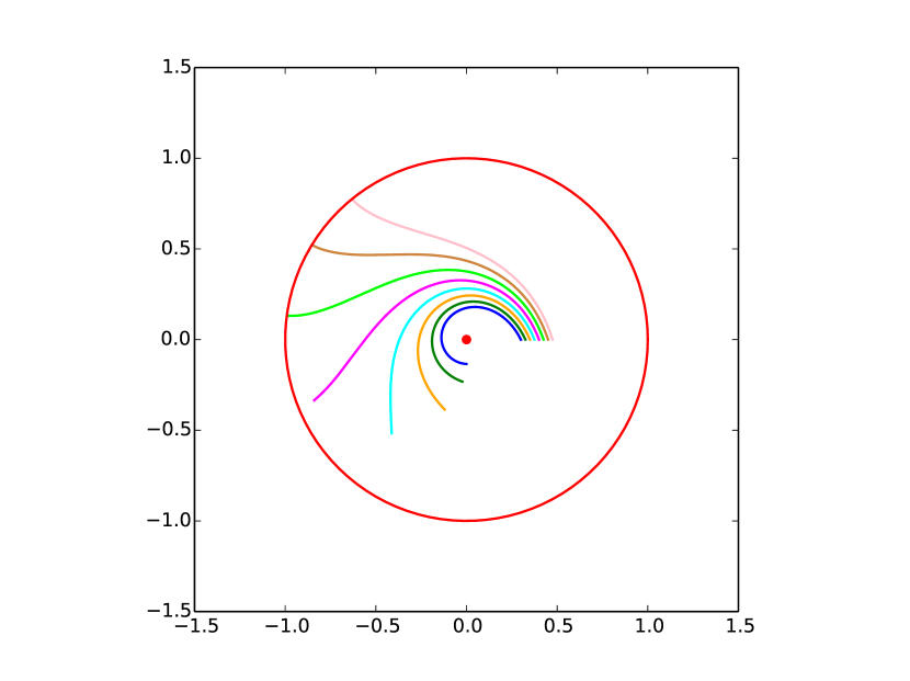
(a) Geodesic segments.

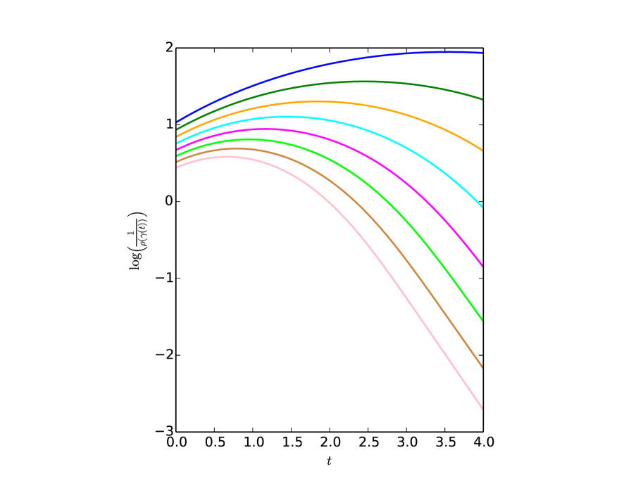
(b) Corresponding (1.2) functions.

Figure 6. Some geodesic segments in the condition metric when $\mathcal{M}$ is the disk model of the hyperbolic plane $\mathbb{H}^{2}$ and $\mathcal{N}$ is the red point, $(0,0)$. Clearly the self-convexity property is not satisfied in this case.

Proof of Theorem 1.3.

Let $\mathbb{D}^{2}$ be the Poincaré disk model for the hyperbolic space, $\mathbb{D}^{2}=\{z\in\mathbb{C}\ |\ |z|<1\}$. We take polar coordinates $(r,\phi)\mapsto re^{i\phi}$ with $r\in(0,1)$ and $\phi\in(-\pi,\pi)$. Then the local expression for the metric tensor is

$$g_{(r,\phi)}=\begin{pmatrix}\frac{1}{(1-r)^{2}}&0\\ 0&\frac{r^{2}}{(1-r)^{2}}\end{pmatrix}.$$

If we take $\mathcal{N}=\{(0,0)\}$, then the (hyperbolic) distance from a point $(r,\phi)$ to $\mathcal{N}$ is $\rho(r,\phi)=-\log(1-r)$. If $(\dot{r},\dot{\phi})$ is a tangent vector at the point $(r,\phi)$, then its norm is given by

(6.1) $$\|(\dot{r},\dot{\phi})\|^{2}_{(r,\phi)}=\frac{\dot{r}^{2}+\dot{\phi}^{2}r^{2}}{(1-r)^{2}}.$$

Now let us compute the Christoffel symbols for the Pincaré disk. We have that

$$\frac{\partial g_{11}}{\partial_{r}}=\frac{2}{(1-r)^{3}}\qquad\frac{\partial g_{22}}{\partial r}=\frac{2r}{(1-r)^{3}},$$

and the rest of the derivatives are zero. The Christoffel symbols are

$$\Gamma_{11}^{1}=\frac{1}{1-r},\qquad\Gamma_{12}^{1}=0,\qquad\Gamma_{22}^{1}=-\frac{r}{1-r},$$

$$\Gamma_{11}^{2}=0,\qquad\Gamma_{12}^{2}=\frac{1}{r(1-r)},\qquad\Gamma_{22}^{2}=0.$$

With the Christoffel symbols we obtain the geodesic equations

(6.2) $$\left\{\begin{array}[]{rl}\ddot{r}+\frac{\dot{r}^{2}}{1-r}-\frac{r\dot{\phi}^{2}}{1-r}&=0\\ \ddot{\phi}+\frac{2\dot{r}\dot{\phi}}{r(1-r)}=0\end{array}\right.$$

Now let us compute the derivatives of the distance function $\rho$. Let $(r,\phi)$ be a point and $(\dot{r},\dot{\phi})$ a tangent vector. Let $c(t)=(c_{1}(t),c_{2}(t))$ be a curve with $c(0)=(r,\phi)$ and $c^{\prime}(0)=(\dot{r},\dot{\phi})$. We have that

$$\frac{d}{dt}\rho(c(t))=\frac{d}{dt}[-\log(1-c_{1}(t))]=\frac{c_{1}^{\prime}(t)}{1-c_{1}(t)}.$$

Hence,

(6.3) $$D\rho_{(r,\phi)}(\dot{r},\dot{\phi})=\frac{\dot{r}}{1-r}.$$

Now let $\gamma(t)=(\gamma_{1}(t),\gamma_{2}(t))$ be a geodesic (w.r.t. the original hyperbolic metric) with $\gamma(0)=(r,\phi)$ and $\gamma^{\prime}(0)=(\dot{r},\dot{\phi})$. Then,

$$\frac{d^{2}}{dt^{2}}\rho(\gamma(t))=\frac{d}{dt}\frac{\gamma_{1}^{\prime}(t)}{1-\gamma_{1}(t)}=\frac{\gamma_{1}^{\prime\prime}(t)(1-\gamma_{1}(t))+\gamma_{1}^{\prime}(t)^{2}}{(1-\gamma_{1}(t))^{2}}.$$

Therefore,

(6.4) $$D^{2}\rho_{(r,\phi)}((\dot{r},\dot{\phi}),(\dot{r},\dot{\phi}))=\frac{\ddot{r}(1-r)+\dot{r}^{2}}{(1-r)^{2}}=\frac{r\dot{\phi}^{2}}{(1-r)^{2}},$$

where we have replaced $\ddot{r}$ by its value in terms of $\dot{r}$ and $\dot{\phi}$ using the geodesic equations (6.2). Let us compute the operator norm of $D\rho_{(r,\phi)}$. The quantity in (6.3) is maximized when $\dot{r}$ is as large as possible. Let us consider the tangent vector $(1,0)$, whose norm is $\frac{1}{1-r}$. Then $(1-r,0)$ is a unitary vector that maximizes $D\rho_{(r,\phi)}$. Hence,

(6.5) $$\|D\rho_{(r,\phi)}\|=D\rho_{(r,\phi)}(1-r,0)=1.$$

Finally, let us compute quantity in Proposition 4.4 using (6.1), (6.3), (6.4) and (6.5).

$$\|(\dot{r},\dot{\phi})\|^{2}\|D\rho_{(r,\phi)}\|^{2}-(D\rho_{(r,\phi)}(\dot{r},\dot{\phi}))^{2}$$

$$-\rho(r,\phi)D^{2}\rho_{(r,\phi)}((\dot{r},\dot{\phi}),(\dot{r},\dot{\phi})) =\frac{\dot{\phi}^{2}r(r+\log(1-r))}{(1-r)^{2}}.$$

Since the real function $r\mapsto r+\log(1-r)<0$ for every $r\in(0,1)$, the quantity above is zero if and only if $\dot{\phi}=0$ ($(\dot{r},\dot{\phi})$ points towards the origin) and otherwise is negative. Proposition 4.4 finishes the proof. ∎

References

- [1] Carlos Beltrán, Jean-Pierre Dedieu, Gregorio Malajovich, and Mike Shub, Convexity properties of the condition number, SIAM J. Matrix Anal. Appl. 31 (2009), no. 3, 1491–1506. MR 2587788 (2011c:65071)
- [2] Carlos Beltrán, Jean-Pierre Dedieu, Gregorio Malajovich, and Mike Shub, Convexity properties of the condition number ii., SIAM J. Matrix Analysis Applications 33 (2012), no. 3, 905–939.
- [3] Carlos Beltrán and Michael Shub, Complexity of bezout’s theorem vii: Distance estimates in the condition metric, Foundations of Computational Mathematics 9 (2009), no. 2, 179–195.
- [4] Carlos Beltrán and Michael Shub, On the geometry and topology of the solution variety for polynomial system solving, Found. Comput. Math. 12 (2012), no. 6, 719–763. MR 2989472
- [5] Paola Boito and Jean-Pierre Dedieu, The condition metric in the space of rectangular full rank matrices, SIAM J. Matrix Anal. Appl. 31 (2010), no. 5, 2580–2602. MR 2740622 (2012e:65078)
- [6] Robert L. Foote, Regularity of the distance function, Proc. Amer. Math. Soc. 92 (1984), no. 1, 153–155. MR 749908 (85m:58024)
- [7] Yanyan Li and Louis Nirenberg, Regularity of the distance function to the boundary, Rend. Accad. Naz. Sci. XL Mem. Mat. Appl. (5) 29 (2005), 257–264. MR 2305073 (2008d:35021)
- [8] Michael Shub, Complexity of bezout’s theorem vi: Geodesics in the condition (number) metric, Foundations of Computational Mathematics 9 (2009), no. 2, 171–178.
- [9] M. P. do Carmo, Riemannian Geometry, Birkhäuser, Boston, MA, (1992)