Bayesian Hypothesis Test using Nonparametric Belief Propagation for Noisy Sparse Recovery

Abstract

This paper proposes a low-computational Bayesian algorithm for noisy sparse recovery (NSR), called BHT-BP. In this framework, we consider an LDPC-like measurement matrices which has a tree-structured property, and additive white Gaussian noise. BHT-BP has a joint detection-and-estimation structure consisting of a sparse support detector and a nonzero estimator. The support detector is designed under the criterion of the minimum detection error probability using a nonparametric belief propagation (nBP) and composite binary hypothesis tests. The nonzeros are estimated in the sense of linear MMSE, where the support detection result is utilized. BHT-BP has its strength in noise robust support detection, effectively removing quantization errors caused by the uniform sampling-based nBP. Therefore, in the NSR problems, BHT-BP has advantages over CS-BP [13] which is an existing nBP algorithm, being comparable to other recent CS solvers, in several aspects. In addition, we examine impact of the minimum nonzero value of sparse signals via BHT-BP, on the basis of the results of [27],[28],[30]. Our empirical result shows that variation of $x_{min}$ is reflected to recovery performance in the form of SNR shift.

I Introduction

I-A Background

Robust reconstruction of sparse signals against measurement noise is a key problem in real-world applications of compressed sensing (CS) [1]-[3]. We refer to such signal recovery problems as noisy sparse signal recovery (NSR) problems. The NSR problems can be directly defined as an $l_{0}$-norm minimization problem [4],[5]. Solving the $l_{0}$-norm task is very limited in practice when the system size $(M,N)$ becomes large. Therefore, several alternative solvers have been developed to relax computational cost of the $l_{0}$-norm task, such as $l_{1}$-norm minimization solvers, e.g., Dantzig selector ($l_{1}$-DS) [6] and Lasso [7], and greedy type algorithms, e.g., OMP [8] and COSAMP [9]. Another popular approach to the computational relaxation is based on the Bayesian philosophy [11]-[17]. In the Bayesian framework, the $l_{0}$-norm task is described as maximum a posteriori (MAP) estimation problem, and sparse solution then is sought by imposing a certain sparsifying prior probability density function (PDF) with respect to the target signal [10].

Recently, Baysian solvers applying belief propagation (BP) have been introduced and caught attention as a low-computational approach to handle the NSR problems in a large system setup [13]-[17]. These BP-based solvers reduce computational cost of the signal recovery by removing unnecessary and duplicated computations using statistical dependency within the linear system. Such BP solvers are also called message-passing algorithms because their recovery behavior is well explained by passing statistical messages over a tree-structured graph representing the statistical dependency [18].

For implementation of BP, two approaches have been mainly discussed according to message representation methods: parametric BP (pBP) [15]-[17],[39],[40] where the BP-message is approximated to a Gaussian PDF; hence, only the mean and variance are used for message-passing, and nonparametric BP (nBP) [13],[14],[19]-[23] where the BP-message is represented by samples of the corresponding PDF. When the pBP approach is used, there are errors from the Gaussian approximation; these errors decrease as problem size $(N,M)$ increases. If the nBP approach is used, there is an approximation error which generally depends upon the choice of message sampling methods.

I-B Contribution

In this paper, a low-computational Bayesian algorithm is developed based on the nBP approach. We refer to the proposed algorithm as Bayesian hypothesis test using nonparametric belief propagation (BHT-BP). Differently from the pBP-based solvers, BHT-BP can precisely infer the multimodally distributed BP-messages via an uniform sampling-based nBP. Therefore, BHT-BP can be applied to any types of sparse signals in the CS framework by adaptively choosing a signal prior PDF. In addition, the proposed algorithm uses low-density parity-check codes [24] (LDPC)-like sparse measurement matrices as works in [13],[15],[16]. Although such sparse matrices perform worse than the dense matrices do in terms of compressing capability in the CS framework, they can highly speed up the generation of the CS measurements [27].

Most CS algorithms to date for the NSR problems have been developed under the auspices of signal estimation rather than support detection. However, recently studies have indicated that the existing estimation-based algorithms, such as Lasso [7], lead to a potentially large gap with respect to the theoretical limit for the noisy support recovery [28]-[30]. Motivated by such theoretical investigation, the proposed BHT-BP takes a joint detection-and-estimation structure [31],[41], as shown in Fig.3, which consists of a sparse support detector and a nonzero estimator. The support detector uses uniform sampling-based nBP and composite binary hypothesis tests to the CS measurements $\mathbf{Z}$ at hand for the sparse support finding. Given the detected support, the underdetermined CS problem is reduced to an overdetermined problem. Then, the nonzero estimator is applied under the criterion of linear minimum mean-square-error (LMMSE) [33]. Then, let us state the detailed novel points of the proposed algorithm. In the CS framework considering reconstruction of a sparse signal $\mathbf{X}\in\mathbb{R}^{N}$ from noisy measurements $\mathbf{Z}\in\mathbb{R}^{M}$, BHT-BP is novel in terms of

1. Providing robust support detection against additive measurement noise based on the criterion of the minimum detection error probability,

2. Removing MSE degradation caused by the message sampling of the uniform sampling-based nBP using a joint detection-and-estimation structure,

3. Handling sparse signals whose minimum nonzero value is regulated by a parameter $x_{\min}\geq 0$, proposing a signal prior PDF for such signals,

4. Providing fast sparse reconstruction with recovery complexity $\mathcal{O}(N\log N+KM)$ where $K$ is the signal sparsity.

For the support detection of BHT-BP, we use a hypothesis-based detector designed under the criterion of the minimum detection error probability [32]. BHT-BP represents the signal support using a binary vector, scalarwisely applying the hypothesis testing to each binary element for the support finding. This hypothesis test is “composite” because the likelihood for the test is associated with the value of each scalar $X_{i}$. Therefore, we calculate the likelihood under the Bayesian paradigm; then, the likelihood for the test is a function of the signal prior and the marginal posterior of $X_{i}$. This is the reason why we refer to our support detection as Bayesian hypothesis test (BHT) detection. BHT-BP has noise robustness, outperforming the conventional algorithms, such as CS-BP [13], in the support detection. In this BHT detection, the nBP part takes a role to provide the marginal posterior of $X_{i}$. Therefore, the advantage of BHT-BP in support detection can be claimed when the BP convergence is achieved with the sampling rate, $\frac{M}{N}$, above a certain threshold.

Typically, recovery performance of the nBP-based algorithms is dominated by the message sampling methods. In the case of CS-BP [13], its performance is corrupted by quantization errors because CS-BP works with the uniform sampling-based nBP such that the signal estimate is directly obtained from a sampled posterior. The joint detection-and-estimation structure of BHT-BP overcomes this weakpoint of CS-BP, improving MSE performance. The key behind the improvement is that the sampled posterior is only used for the support detection in BHT-BP. Furthermore, BHT-BP closely approaches to the oracle performance, in high SNR regime, if the rate $\frac{M}{N}$ are sufficiently maintained for the signal sparsity $K$. Fig.1 is an illustration intended to see a motivational evidence of the recovery performance among the proposed BHT-BP, CS-BP [13] and BCS [12].

The importance of the minimum nonzero value $x_{\min}$ of sparse signals $\mathbf{X}$ in the NSR problems was highlighted by Wainwright et al. in [27],[28] and Fletcher et al. in [30], where they proved that the perfect support recovery is very difficult even with arbitrarily large signal-to-noise ratio (SNR) if $x_{min}$ is very small. Following these works, in the present work, we consider recovery of $\mathbf{X}$ whose minimum nonzero value is regulated by $x_{min}$. In addition, we propose to use a signal prior including the parameter $x_{min}$, called spike-and-dented slab prior, investigating how the performance varies according to the parameter $x_{min}$. We empirically show in the BHT-BP recovery that variation of $x_{min}$ is reflected to the recovery performance in the form of SNR shift. In addition, we support this statement with a success rate analysis for the BHT support detection under the identity measurement matrix assumption, i.e., $\mathbf{\Phi}=\mathbf{I}$.

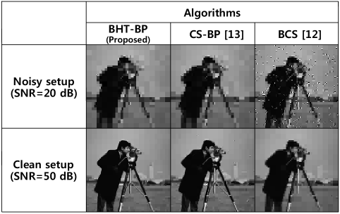
Figure 1: An illustrative recovery example of BHT-BP (the proposed), CS-BP [13] and BCS [12] in the presence of noise. The original image, known as the Cameraman, of size $N=128^{2}$, is transformed via three step discrete wavelet transform. For this example, we pad zeros for the coefficients having values below $100$ in wavelet domain, and we recover these images from $M/N=0.5$ undersampled measurements. From this example, we see that the recovered image via BCS includes flicker noise but which is not shown in that of BHT-BP in the noisy setup. In the clean setup, BHT-BP more clearly recovers the image than those of CS-BP and BCS.

The recovery complexity of BHT-BP is $\mathcal{O}(N\log N+KM)$ which includes the cost $\mathcal{O}(KM)$ of the LMMSE estimation and that of the BHT support detection $\mathcal{O}(N\log N)$. This is advantageous compared to that of the $l_{1}$-norm solvers $\Omega(N^{3})$ [6],[7] and BCS $\mathcal{O}(NK^{2})$ [12], being comparable to that of the recent BP-based algorithms using sparse measurement matrices $\mathcal{O}(N\log N)$: CS-BP [13] and SuPrEM [16].

I-C Organization

The remainder of the paper is organized as follows. We first provide basic setup for our work in Section II. In Section III, we discuss our solution approach to the NSR problem. Section IV describes a nonparametric implementation of the BHT support detector and its computational complexity. Section V provides experimental validation to show performance and several aspects of the proposed algorithm, compared to the other related algorithms. Finally, we conclude this paper in Section VI.

II Basic Setup

In this section, we introduce our signal model, and a factor graphical model for linear systems used in this work.

II-A Signal Model

Let $\mathbf{x}_{0}\in\mathbb{R}^{N}$ denote a sparse vector which is a deterministic realization of a random vector $\mathbf{X}$. Here, we assume that the elements of $\mathbf{X}$ are i.i.d., and each $X_{i}$ belongs to the support set with a sparsity rate $q\in[0,1)$. To indicate the supportive state of $\mathbf{X}$, we use a state vector $\mathbf{S}\in\{0,1\}^{N}$ whose each element $S_{i}$ is Bernoulli random with the rate $q$ as following

$${S_{i}}=\left\{\begin{array}[]{l}1,\,\,\,\,\,{\rm{if}}\,\,X_{i}\neq 0\text{ with }q\\ 0,\,\,\,\,\,{\rm{if}}\,\,X_{i}=0\text{ with }1-q\end{array}\right..$$ (3)

Then, the signal sparsity, $K=||\mathbf{S}||_{0}$, becomes Binomial random with $\mathcal{B}(k;N,q)$. In the present work, we consider the signal $\mathbf{x}_{0}$ whose minimum nonzero value is regulated by a parameter $x_{min}\geq 0$. For such signal generation,

• We first draw a state vector $\mathbf{s}$ by generating $N$ i.i.d. Bernoulli numbers of (3).

• Then, we assign zero value to the signal scalars corresponding to $s_{i}=0$, i.e., $x_{0,i}=0$.

• For the signal scalar corresponding to $s_{i}=1$, a Gaussian number is drawn from $\mathcal{N}(x;0,\sigma_{X}^{2})$ and assigned to the signal scalar $x_{0,i}$ if $|x_{0,i}|\geq x_{min}$; otherwise, the number is redrawn until a realization with $|x_{0,i}|\geq x_{min}$ occurs.

For such signals with $x_{min}$, we propose to use a spike-and-dented slab prior which is a variant of the spike-and-slab prior [36]. According to (3), the signal prior of $X_{i}$ can be described as a two-state mixture PDF with the state $S_{i}$, i.e.,

$$f_{X_{i}}(x)=(1-q)f_{X_{i}}(x|S_{i}=0)+qf_{X_{i}}(x|S_{i}=1).$$ (4)

Then, the spike-and-dented slab prior includes the conditional priors as following

$${f_{{X_{i}}}}(x|{S_{i}}=0)=\delta(x),$$ (5)

$${f_{{X_{i}}}}(x|{S_{i}}=1)\propto\left\{\begin{gathered}\mathcal{N}(x;0,\sigma_{X}^{2}),\,\,\,|x|\geq{x_{\min}}\hfill\\ \lambda,\,\,\,\,\,\,\,\,\,\,\,\,\,\,\,\,\,\,\,\,\,\,\,\,\,\,\,\,\,|x|<{x_{\min}}\hfill\\ \end{gathered}\right.$$ (8)

where $\delta(x)$ is the Dirac delta PDF and $\lambda>0$ is a near-zero constant. Fig.2 shows an example of the spike-and-dented slab prior where the prior is drawn with the parameters, $q=0.05,\sigma_{X}=5,x_{\min}=\frac{\sigma_{X}}{4},\lambda=10^{-4}$, and normalized to be $\int_{{X_{i}}}{{f_{{X_{i}}}}(x)dx=1}$.

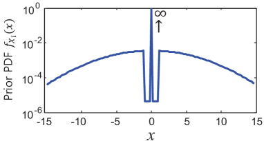
Figure 2: Example of spike-and-dented slab PDF in log-scale where the prior is drawn with the parameters, $q=0.05,\sigma_{X}=5,x_{\min}=\frac{\sigma_{X}}{4},\lambda=10^{-4}$, and normalized to be $\int_{{X_{i}}}{{f_{{X_{i}}}}(x)dx=1}$.

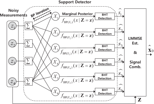
Figure 3: Diagrammatic representation of the proposed algorithm (when $N=6,M=4,L=2$) where the inputs of the proposed algorithm is the measurement $\mathbf{z}=[z_{1},z_{2},z_{3},z_{4}]$ and the output is a signal estimate $\widehat{\mathbf{x}}_{0}$. The proposed algorithm first detects the signal support $\widehat{\mathbf{s}}=[\widehat{s}_{1},...,\widehat{s}_{6}]$ from the measurements $\mathbf{z}$ at hand, and then applies linear MMSE estimation to find the signal estimate $\widehat{\mathbf{x}}_{0}$ given the detected support $\widehat{\mathbf{s}}$.

The goal of the proposed algorithm is to recover the signal vector $\mathbf{x}_{0}$ from a noisy measurement vector

$$\mathbf{z}=\mathbf{\Phi}\mathbf{x}_{0}+\mathbf{w}\in\mathbb{R}^{M},$$ (9)

given a fat measurement matrix $\mathbf{\Phi}\in\{0,1,-1\}^{M\times N}$ $(M<N)$, where the vector $\mathbf{w}\in\mathbb{R}^{M}$ is a realization of a Gaussian random vector $\mathbf{W}\sim{\mathcal{N}(\mathbf{w};0,\sigma_{W}^{2}\mathbf{I})}$; therefore, the vector $\mathbf{z}\in\mathbb{R}^{M}$ is drawn from a mean shifted Gaussian random vector conditioned on $\mathbf{X}=\mathbf{x}_{0}$, i.e., $\mathbf{Z}\sim{\mathcal{N}(\mathbf{z};\mathbf{\Phi}\mathbf{x}_{0},\sigma_{W}^{2}\mathbf{I})}$. For the measurement matrix $\mathbf{\Phi}$, we consider an LDPC-like sparse matrix which has very low matrix sparsity (typically less than 1$\%$ matrix sparsity) and the tree-structured property [25],[26]. We regulate the matrix sparsity by the fixed column weight $L$ such that $\mathbb{E}[\left\|{{\phi_{\text{column}}}}\right\|_{2}^{2}]=L$. This regulation enables the matrix $\mathbf{\Phi}$ to span the measurement space with column vectors having equal energy.

II-B Factor Graphical Modeling of Linear Systems

Factor graphs effectively represent such sparse linear systems in (9) [18]. Let $\mathcal{V}:=\{1,...,N\}$ denote a set of variable nodes corresponding to the signal elements, $\mathbf{x}_{0}=[x_{0,1},...,x_{0,N}]$, and $\mathcal{C}:=\{1,...,M\}$ denote a set of factor nodes corresponding to the measurement elements, $\mathbf{z}=[z_{1},...,z_{M}]$. In addition, we define a set of edges connecting $\mathcal{V}$ and $\mathcal{C}$ as $\mathcal{E}:=\{(j,i)\in\mathcal{C}\times\mathcal{V}\,|\,\,\phi_{ji}=1\}$ where $\phi_{ji}$ is the $(j,i)$-th element of $\mathbf{\Phi}$. Then, a factor graph $\mathcal{G}=(\mathcal{V,C,E})$ fully describes the neighboring relation in the sparse linear system. For convenience, we define the neighbor set of $\mathcal{V}$ and $\mathcal{C}$ as $N_{\mathcal{V}}(i):=\{j\in\mathcal{C}\,|(j,i)\in{\mathcal{E}}\}$ and $N_{\mathcal{C}}(j):=\{i\in\mathcal{V}\,|(j,i)\in{\mathcal{E}}\}$, respectively. Note that the column weight of the matrix $\mathbf{\Phi}$ is expressed as $L=\left|N_{\mathcal{V}}(i)\right|$ in this graph model.

III Solution Approach of Proposed Algorithm

The proposed algorithm, BHT-BP, has a joint detection-and-estimation structure where we first detect the sparse support by a combination of BP and BHT, then estimating nonzeros in the detected support by an LMMSE estimator, as shown in Fig.3. In this section, we provide our solution approach to the support detection and the nonzero estimation under the joint structure.

III-A Support Detection using Bayesian Hypothesis Testing

III-A1 Support detection in BHT-BP

The support detection problems can be decomposed to a sequence of binary state detection problems given the marginal posterior $f_{{X_{i}}}(x|{\bf{Z}}={\bf{z}})$ of each signal scalar. Our state detection problem is to choose one between the two hypotheses:

$$\begin{array}[]{l}\mathcal{H}_{0}:S_{i}=0\,\,\,\text{and}\,\,\,\mathcal{H}_{1}:S_{i}=1,\end{array}$$

given the measurements $\mathbf{z}$. Our methodlogy to this problem is related to Bayesian composite hypothesis testing [32, p. 198]. In contrast to the simple hypothesis test where the PDFs under both hypothesis are perfectly specified, the composite hypothesis test must consider associated random variables. In our problem, the associated random variable is $X_{i}$. Then, the binary state detector decides $\mathcal{H}_{1}$ if

$$\frac{{{f_{\mathbf{Z}}}({\mathbf{z}}|{\mathcal{H}_{1}})}}{{f_{\mathbf{Z}}}({\mathbf{z}}|{\mathcal{H}_{0}})}=\frac{{\int{{{f_{\mathbf{Z}}}({\mathbf{z}}|{\mathcal{H}_{1}},{X_{i}}=x)}{f_{{X_{i}}}}(x|{\mathcal{H}_{1}})dx}}}{{\int{{{f_{\mathbf{Z}}}({\mathbf{z}}|{\mathcal{H}_{0}},{X_{i}}=x)}{f_{{X_{i}}}}(x|{\mathcal{H}_{0}})dx}}}>\gamma,$$ (10)

where $\gamma$ is a threshold for the test. The PDF ${{f_{\mathbf{z}}}({\mathbf{z}}|{\mathcal{H}_{s_{i}}},{X_{i}}=x)}$ is simplified to ${{f_{\mathbf{Z}}}({\mathbf{z}}|{X_{i}}=x)}$ since the hypothesis $\mathcal{H}_{s_{i}}$ and the measurements $\mathbf{Z}$ are conditionally independent given $X_{i}$. Therefore, finally, the binary hypothesis test in (10) can be rewritten as

$$T_{\text{\tiny BHTBP}}(\mathbf{z}):=\frac{{\int{\frac{{{f_{{X_{i}}}}(x|S_{i}=1)}}{{{f_{{X_{i}}}}(x)}}{f_{{X_{i}}}}(x|{\mathbf{Z}}={\mathbf{z}})dx}}}{{\int{\frac{{{f_{{X_{i}}}}(x|S_{i}=0)}}{{{f_{{X_{i}}}}(x)}}{f_{{X_{i}}}}(x|{\mathbf{Z}}={\mathbf{z}})dx}}}\mathop{\mathop{\gtrless}\limits_{{\mathcal{H}_{0}}}}\limits^{{\mathcal{H}_{1}}}\gamma$$ (11)

where the Bayesian rule is applied to ${{f_{\mathbf{Z}}}({\mathbf{z}}|{X_{i}}=x)}=\frac{{{f_{{X_{i}}}}(x|{\mathbf{Z}}={\mathbf{z}}){f_{{\mathbf{Z}}}}(\mathbf{z})}}{{{f_{{X_{i}}}}(x)}}$, and obviously ${f_{{X_{i}}}}(x|{\mathcal{H}_{s_{i}}})={f_{{X_{i}}}}(x|S_{i}=s_{i})$ holds from the prior knowledge of (4).

Figure 4: Fig.4 illustrates the scalar state detection by BHT under an assumption of $\mathbf{\Phi}=\mathbf{I}$. Under this assumption, “the hypothesis test given a vector $\mathbf{z}$” is simplified to “the test given a scalar $z_{j}$”, described in (13), where the threshold $\gamma^{\prime}$ is derived from the equality condition of (14). In the figure, the horizontal-lined region (blue) represents $\Pr\{{\widehat{s}_{i}}\neq{s_{i}}|{\mathcal{H}_{1}}\}$ and the vertical-lined (red) region does $\Pr\{{\widehat{s}_{i}}\neq{s_{i}}|{\mathcal{H}_{0}}\}$.

In some detection problem under Bayesian paradigm, one can reasonably assign prior probabilities to the hypotheses. In the present work, we assign the sparsity rate $q$ to the hypotheses, i.e., $\Pr\{\mathcal{H}_{0}\}=1-q$ and $\Pr\{\mathcal{H}_{1}\}=q$. Then, we can define the state error rate (SER) of the scalar state detection (11) [32, p. 78]

$${P_{\text{SER}}}:=\Pr\{{\widehat{s}_{i}}\neq{s_{i}}|{\mathcal{H}_{0}}\}(1-q)+\Pr\{{\widehat{s}_{i}}\neq{s_{i}}|{\mathcal{H}_{1}}\}q.$$ (12)

It is well known that the threshold $\gamma$ of (11) can be optimized under the criterion of the minimum detection error probability with the SER expression (12). By the criterion, we assign the threshold to $\gamma=\gamma^{*}:=\frac{1-q}{q}$. We omit the derivation for this threshold optimization here, referring interested readers to [32, p. 90]. We call this binary hypothesis test (11) with the threshold $\gamma^{*}$ as Bayesian hypothesis test (BHT) detection. The proposed algorithm generates a detected support $\widehat{\mathbf{s}}\in\{0,1\}^{N}$ according to the results of a sequence of BHTs. Therefore, given a marginal posterior of each $X_{i}$, BHT-BP can robustly detect the signal support even when the measurements are noisy.

Fig.4 illustrates the scalar state detection of BHT-BP when the matrix is $\mathbf{\Phi}=\mathbf{I}$ such that the measurement channel can be decoupled to $N$ scalar Gaussian channels, i.e., $Z_{j}=X_{i}+W_{j},\,(i=j)$. Under this assumption, “the hypothesis test given a vector $\mathbf{z}$” can be scalarwise to “the test given a scalar $z_{j}$”, being simplified

$$\forall j\in\mathcal{C}:|z_{j}|\mathop{\mathop{\gtrless}\limits_{{\mathcal{H}_{0}}}}\limits^{{\mathcal{H}_{1}}}\gamma^{\prime}$$ (13)

where the threshold $\gamma^{\prime}$ is derived from the equality condition with the two scalar likelihood and the threshold $\gamma^{*}=\frac{1-q}{q}$,

$$\frac{{{f_{Z_{j}}}(z|{\mathcal{H}_{1}})}}{{f_{Z_{j}}}(z|{\mathcal{H}_{0}})}=\gamma^{*}.$$ (14)

Hence, the threshold $\gamma^{\prime}$ is a function of $\sigma_{X}$, $\sigma_{W}$, $x_{\min}$, and $q$ (see Appendix II). With this threshold $\gamma^{\prime}$, we can find the conditional SER, $\Pr\{{\widehat{s}_{i}}\neq{s_{i}}|{\mathcal{H}_{s_{i}}}\}$, for the case $\mathbf{\Phi}=\mathbf{I}$. In Fig.4, the horizontal-lined region (blue) represents $\Pr\{{\widehat{s}_{i}}\neq{s_{i}}|{\mathcal{H}_{1}}\}$ and the vertical-lined (red) region does $\Pr\{{\widehat{s}_{i}}\neq{s_{i}}|{\mathcal{H}_{0}}\}$. The corresponding SER analysis will be provided in Appendix II. Although Fig.4 does not show typical behavior of the BHT detection given a vector measurement $\mathbf{z}$, the figure helps intuitive understanding of the BHT detection.

In addition, it is noteworthy in Fig.4 that the shape of ${f_{Z_{j}}}(z|{\mathcal{H}_{1}})$ is dented near $z_{j}=0$. This is caused by the use of the spike-and-dented slab prior, given in (5), where the dented part varies with the parameter $x_{\min}$.

III-A2 Support detection of CS-BP

Support detection is not performed in practical recovery of CS-BP, but we describe it here for a comparison purpose. CS-BP estimates the sparse solution $\widehat{\mathbf{x}}_{0}$ directly from a BP approximation of the signal posterior, through MAP or MMSE estimation. Let us consider CS-BP using the MAP estimation. Then, given the marginal posterior $f_{{X_{i}}}(x|{\bf{Z}}={\bf{z}})$, the scalar state detection of CS-BP is equivalent to choose one of the two peaks at $x=0$ and $x=\widehat{x}_{\text{MAP},i}:=\arg\mathop{\max}\limits_{x}f_{{X_{i}}}(x|{\bf{Z}}={\bf{z}})$. Namely, the binary state detector of CS-BP decides $\mathcal{H}_{1}$ if

$$T_{\text{\tiny CSBP}}(\mathbf{z}) :=\frac{{\Pr\{\widehat{x}_{\text{MAP},i}-\Delta x<{X_{i}}\leq\widehat{x}_{\text{MAP},i}+\Delta x|\mathbf{Z}=\mathbf{z}\}}}{{\Pr\{0-\Delta x<{X_{i}}\leq 0+\Delta x|\mathbf{Z}=\mathbf{z}\}}}$$

$$=\frac{{\int_{\widehat{x}_{\text{MAP},i}-\Delta x}^{\widehat{x}_{\text{MAP},i}+\Delta x}{f_{{X_{i}}}(x|{\bf{Z}}={\bf{z}})dx}}}{{\int_{0-\Delta x}^{0+\Delta x}f_{{X_{i}}}(x|{\bf{Z}}={\bf{z}})dx}}>1,$$ (15)

where $\Delta x$ is a small quantity that we eventually let approach to 0. When $\widehat{x}_{\text{MAP},i}=0$, the test cost becomes one; then, the detector immediately decides $\mathcal{H}_{0}$. Hence, in CS-BP, the detected support $\mathbf{\widehat{s}}$ is just a by-product of the signal estimate $\widehat{\mathbf{x}}_{\text{MAP}}$, which is not robust support detection against additive measurement noise.

III-B Conditions for BP Convergence

In the proposed algorithm, marginal posterior of each $X_{i}$, $f_{X_{i}}(x|\mathbf{Z}=\mathbf{z})$, for the BHT detection is computed by BP. It was known that BP efficiently computes such marginal posteriors, achieving its convergence if the conditions in Note 1 are satisfied [42]. Given the BP convergence, each approximate marginal posterior converges to a PDF peaked at an unique value $\widehat{x}_{i}$ during the iteration. In noiseless setup, the unique value is exactly the true value, i.e., $\widehat{x}_{i}=x_{0,i}$.

Note 1 (Conditions for BP convergence):

• The factor graph, which corresponds to the relation between $\mathbf{X}$ and $\mathbf{Z}$, has a tree-structure.

• Sufficiently large number of iterations $l$ is maintained such that BP-messages have been propagated along every link of the tree, and a variable node has received messages from all the other variables nodes.

Although the second condition in Note 1 is practically demanding, it has been reported that BP provides a good approximation of marginal posteriors even with factor graphs including cycles, which is called loopy BP [25],[39],[40].

A related argument for BP was stated by Guo and Wang in the context of the multiuser detection problem of CDMA systems, where the problem is actually equivalent to solve a linear system [37],[38]. In the works, Guo and Wang showed that the marginal posterior computed by BP is almost exact in a large linear system ($M,N\to\infty$) if the factor graph corresponding to the matrix $\mathbf{\Phi}$ is asymptotically cycle-free and the sampling rate $\frac{M}{N}$ is above a certain threshold. Namely, Guo and Wang showed that

$$\mathop{\lim}\limits_{l\to\infty}\mathop{\lim\sup}\limits_{M,N\to\infty}\left|{f_{\text{BP}({X_{i}})}^{(l)}(x|{\bf{Z}}={\bf{z}})-f_{{X_{i}}}(x|{\bf{Z}}={\bf{z}})}\right|=0,$$ (16)

where $f_{\text{BP}({X_{i}})}^{(l)}(x|{\bf{Z}}={\bf{z}})$ is an approximate marginal posterior of each $X_{i}$ by $l$ iterations of BP.

According to the literature, in the linear system with the LDPC-like matrix $\mathbf{\Phi}$, the sampling rate $\frac{M}{N}$ is the only obstacle for the BP convergence. The asymptotic condition used in (16) is not always necessary if the tree-structured property is guaranteed for the matrix $\mathbf{\Phi}$ because the main reason to use the asymptotic condition in the works of [37],[38] is to make the system “asymptotically cycle-free”, which is equivalent to having an “asymptotically tree-structured” matrix $\mathbf{\Phi}$. Thus, we claim the advantage of BHT-BP over CS-BP in support detection with a certain threshold of the rate $\frac{M}{N}$. Given $\frac{M}{N}$ below the threshold, the BP convergence is not achieved such that the likelihood $f_{\mathbf{Z}}(\mathbf{z}|\mathcal{H}_{s_{i}})$ is not properly calculated for the BHT detection. We will empirically find the threshold using information entropy of the approximate marginal posterior, $f_{\text{BP}({X_{i}})}^{(l)}(x|{\bf{Z}}={\bf{z}})$, in Section V-A. Although we do not provide an analytical threshold of $\frac{M}{N}$ for the BP convergence in this paper, simulation results with $\frac{M}{N}$ above the empirical threshold are quite favorable, as shown in Section V-B and -C.

III-C LMMSE Estimation of Nonzero Values

Given the support information by the BHT detection, the rest of the work is reduced to the nonzero estimation problem, represented as

$${\widehat{\bf{x}}_{0}}=\mathbb{E}\left[{{{\bf{X}}}|{\bf{S}}={\widehat{\bf{s}}},{\bf{Z}}={\bf{z}}}\right],$$ (17)

and it can straightforwardly solved by combining the nonzero position by $\widehat{\mathbf{s}}$ and the nonzero values given by the LMMSE estimate [33, p. 364]

$${\widehat{\bf{x}}_{0,\widehat{\bf{s}}}}={\left({\frac{1}{{\sigma_{X}^{2}}}{\bf{I}}+\frac{1}{{\sigma_{W}^{2}}}{\bf{\Phi}}_{\widehat{\bf{s}}}^{T}{\bf{\Phi}}_{\widehat{\bf{s}}}}\right)^{-1}}\frac{1}{{\sigma_{W}^{2}}}{\bf{\Phi}}_{\widehat{\bf{s}}}^{T}\mathbf{z},$$ (18)

where $\mathbf{\Phi}_{\widehat{\mathbf{s}}}\in\{0,1\}^{M\times K}$ denotes a submatrix of $\mathbf{\Phi}$ that contains only the columns corresponding to the detected support $\widehat{\mathbf{s}}$, $\sigma_{X}^{2}$ are the variance of an nonzero scalar $X_{i}$.

The estimate ${\widehat{\bf{x}}_{0}}$ from the proposed joint detection-and-estimation structure is not optimal. As we have seen, our support detector (11) is based on the criterion of minimum detection error probability. Even with this detector, however, we cannot guarantee the estimation optimality since the LMMSE estimator of (17) is not designed from the cost function involving the detection part [31],[41]. Nevertheless, worth mentioning here is that the proposed joint structure has advantages as given in Note 2.

Note 2 (Claims from the joint detection-and-estimation structure):

• Removing the MSE degradation caused by the uniform sampling-based nBP.

• Achieving the oracle performance in the high SNR regime with the sufficiently high rate $\frac{M}{N}$ for the BP convergence.

We will empirically validate this claim in Section V-C.

IV Nonparametric Implementation of BHT Support Detector

This section describes a nonparametric implementation of the proposed support detector consisting of BP and the BHT detection. We discuss our nonparametric approach of the BP part first, and then explain the BHT detection part. This BHT support detection is summarized in Algorithm 1.

IV-A Nonparametric BP using Uniform Sampling

In the BHT support detector, the BP part provides the marginal posterior of $X_{i}$ for the hypothesis test in (11). Since the signal $\mathbf{x}_{0}$ is real valued, each BP-message takes the form of a PDF, and the BP-iteration becomes a density-message-passing process. To implement the density-message-passing, we take the nBP approach [19]-[22]. Many nBP algorithms have been proposed according to several message sampling methods such as discarding samples having low probability density [20], adaptive sampling [21], Gibbs sampling [19], rejection sampling [22], or importance sampling [23].

Our nBP approach is to use an uniform sampling for the message representation where we set the sampling step $T_{s}$ on the basis of the three sigma-rule [35] such that

$$T_{s}=\frac{2\cdot 3\sigma_{X}}{N_{d}}$$ (19)

where $N_{d}$ is the number of samples to store a BP-message. Then, we define the uniform sampling of a density-message $f(x)$ as

$${\rm{Samp}}\left\{{f(x)};T_{s}\right\} :=f(m{T_{s}}-3{\sigma_{X}})$$

$$=f[m],\,\,{\rm{for}}\,\,m\in\{0,1,...,{N_{d}}-1\},$$ (20)

where $\rm{Samp}\left\{\cdot;T_{s}\right\}$ denotes the uniform sampling function with the step size $T_{s}$. Hence, the sampled message $f[m]$ can be treated as a vector with size $N_{d}$ by omitting the index $m$. The main strength of the uniform sampling-based nBP is adaptivity to various signal prior PDFs. In addition, we note that the calculation of uniformly sampled messages can be accelerated using the Fast fourier transform (FFT).

Consider the factor graph $\mathcal{G}=(\mathcal{V,C,E})$ depicted in the support detection part of Fig.3 where a signal element $X_{i}$ corresponds to a variable node $i\in\mathcal{V}$ and a measurement element $Z_{j}$ corresponds to a factor node $j\in\mathcal{C}$. At every iteration, messages are first passed from each variable node $i\in\mathcal{V}$ to its neighboring factor nodes $N_{\mathcal{V}}(i)$; each factor nodes $j\in\mathcal{C}$ then calculates messages to pass back to the neighboring variable nodes $N_{\mathcal{C}}(j)$ based on the previously received messages. These factor-to-variable (FtV) messages include extrinsic information of $X_{i}$, and will then be employed for the computation of updated variable-to-factor (VtF) messages in the next iteration. (For the detail, see the paper [18]).

Let $\mathbf{a}_{i\rightarrow j}^{(l)}\in[0,1)^{N_{d}}$ denote a sampled VtF message at the $l$-th iteration in the vector form, given as

$$\mathbf{a}_{i\rightarrow j}^{(l)}=\eta\left[{{\mathbf{p}_{X_{i}}}\times\prod\limits_{k\in N_{\mathcal{V}}(i)\backslash\{j\}}{{\bf{b}}_{k\rightarrow i}^{(l-1)}}}\right]\,\,\forall(j,i)\in\mathcal{E},$$ (21)

where all product operations are elementwise, the vector $\mathbf{p}_{X_{i}}\in[0,1)^{N_{d}}$ denotes the sampled signal prior, i.e., $\mathbf{p}_{X_{i}}:=\text{Samp}\{f_{X_{i}}(x),T_{s}\}$, and $\eta[\cdot]$ is a normalization function to make $\sum{\mathbf{a}_{i\rightarrow j}^{(l)}}=1$. The sampled FtV message at the $l$-th iteration, $\mathbf{b}_{j\rightarrow i}^{(l)}\in[0,1)^{N_{d}}$, is defined as

$$\mathbf{b}_{j\rightarrow i}^{(l)}=\mathbf{p}_{Z_{j}|\mathbf{X}}\otimes\left(\bigotimes\limits_{k\in N_{\mathcal{C}}(j)\backslash\{i\}}{\mathbf{a}_{k\rightarrow j}^{(l)}}\right)\,\,\forall(j,i)\in\mathcal{E},$$ (22)

where $\otimes$ is the operator for the linear convolution of vectors, and the vector $\mathbf{p}_{Z_{j}|\mathbf{X}}\in[0,1)^{N_{d}}$ is the sampled measurement PDF, i.e., $\mathbf{p}_{Z_{j}|\mathbf{X}}:=\text{Samp}\{\mathcal{N}(z_{j};(\mathbf{\Phi}\mathbf{X})_{j},\sigma_{W}^{2}),T_{s}\}$.

The convolution operations in (22) can be efficiently computed by using FFT. Accordingly, we can rewrite the FtV message calculation as

$${\bf{b}}_{j\to i}^{(l)}=\mathcal{F}^{-1}\left\{\mathcal{F}\mathbf{p}_{Z_{j}|\mathbf{X}}\times\left(\prod\limits_{k\in N_{\mathcal{C}}(j)\backslash\{i\}}{\mathcal{F}\mathbf{a}_{k\rightarrow j}^{(l)}}\right)\right\}$$ (23)

where $\mathcal{F}$ denotes the FFT operation. Therefore, for efficient use of FFT, the sampling step $T_{s}$ should be appropriately chosen such that $N_{d}$ is power of two. In fact, the use of FFT brings a small calculation gap since the FFT-based calculation performs a circular convolution. However, this gap can be ignored, especially when the messages take the form of bell-shaped PDFs such as Gaussian PDFs.

The sampled approximation of the marginal posterior of each $X_{i}$, i.e., $\mathbf{p}_{X_{i}|\mathbf{Z}}^{(l)}:=\text{Samp}\{f_{\text{BP}(X_{i})}^{(l)}(x|\mathbf{Z}=\mathbf{z}),T_{s}\}$, is produced by using the FtV message (22) for every $i\in\mathcal{V}$. Namely,

$$\mathbf{p}_{X_{i}|\mathbf{Z}}^{(l)}=\eta\left[{{\mathbf{p}_{X_{i}}}\times\prod\limits_{k\in N_{\mathcal{V}}(i)}{{\bf{b}}_{k\rightarrow i}^{(l-1)}}}\right]\,\,\forall i\in\mathcal{V},$$ (24)

To terminate the BP loop, we test the condition at every iteration, which is given as

$$\frac{1}{N}\sum\limits_{i=1}^{N}{\frac{{\|{{\bf{p}}_{{X_{i}}|{\bf{Z}}}^{(l)}-{\bf{p}}_{{X_{i}}|{\bf{Z}}}^{(l-1)}}\|_{2}^{2}}}{{\|{{\bf{p}}_{{X_{i}}|{\bf{Z}}}^{(l)}}\|_{2}^{2}}}}\leq\varepsilon$$ (25)

where $\varepsilon>0$ is a constant for the termination condition. If the condition given in (25) is satisfied, the BP loop will be terminated. After the BP termination, we can simply express the marginal posterior of $X_{i}$ by dropping out the iteration index $l$, i.e., ${\bf{p}}_{{X_{i}}|{\bf{Z}}}$.

Algorithm 1 BHT support detection

Noisy measurements $\mathbf{z}$, measurement matrix $\mathbf{\Phi}$, sparsity rate $q$, sampled prior PDF $\mathbf{p}_{X}$, sampled measurement PDF $\mathbf{p}_{Z_{j}|\mathbf{X}}$, The number of samples $N_{d}$, Termination condition $\varepsilon$.

Reconstructed signal $\widehat{\mathbf{x}}_{0}$, Detected support vector $\widehat{\mathbf{s}}$.

1) Belief propagation:

set $\mathbf{b}_{j\rightarrow i}^{(l=0)}=\mathbf{1}\text{ for all }(j,i)\in\mathcal{E}$

while $\frac{1}{N}\sum\limits_{i=1}^{N}{\frac{{\left\|{{\bf{p}}_{{X_{i}}|{\bf{Z}}}^{(l)}-{\bf{p}}_{{X_{i}}|{\bf{Z}}}^{(l-1)}}\right\|_{2}^{2}}}{{\left\|{{\bf{p}}_{{X_{i}}|{\bf{Z}}}^{(l)}}\right\|_{2}^{2}}}}>\varepsilon$ do

$\forall(j,i)\in\mathcal{E}$:

     set $\mathbf{a}_{i\rightarrow j}^{(l)}=\eta\left[{{\mathbf{p}_{X_{i}}}\times\prod\limits_{k\in N_{\mathcal{V}}(i)\backslash\{j\}}{{\bf{b}}_{k\rightarrow i}^{(l-1)}}}\right]$

     set $\mathbf{b}_{j\rightarrow i}^{(l)}=\mathbf{p}_{Z_{j}|\mathbf{X}}\otimes\left(\bigotimes\limits_{k\in N_{\mathcal{C}}(j)\backslash\{i\}}{\mathbf{a}_{k\rightarrow j}^{(l)}}\right)$

$\forall i\in\mathcal{V}$:

     set $\mathbf{p}_{X_{i}|\mathbf{Z}}^{(l)}=\eta\left[{{\bf{a}}_{i\to j^{*}}^{(l)}\times{\bf{b}}_{j^{*}\to i}^{(l-1)}}\right]$

end while

2) BHT detection:

$\forall i\in\mathcal{V}$:

if $\log\frac{{\sum{{{\bf{r}}_{1}}\times{{\bf{p}}_{{X_{i}}|{\bf{Z}}}}}}}{{\sum\limits{{{\bf{r}}_{0}}\times{{\bf{p}}_{{X_{i}}|{\bf{Z}}}}}}}\mathop{>}\log\frac{{1-q}}{q}$ then set $\widehat{s}_{i}=1$

else set $\widehat{s}_{i}=0$

end if

TABLE I: List of algorithms in the performance validation

Algorithms	Complexity	Type of $\Phi$	Type of Prior PDFs	Utilized Techniques
BHT-BP (Proposed)	$\mathcal{O}(N\log N+KM)$	LDPC-like	Spike-and-dented slab	nBP
CS-BP [13]	$\mathcal{O}(N\log N)$	LDPC-like	Spike-and-dented slab	nBP
SuPrEM [16]	$\mathcal{O}(N\log N)$	LDF	Two-layer Gaussian with Jeffery	EM, pBP
BCS [12]	$\mathcal{O}(NK^{2})$	LDPC-like	Two-layer Gaussian with Gamma	EM
$l_{1}$-DS [6]	$\Omega(N^{3})$	Std. Gaussian	-	CVX opt.

IV-B BHT Detection using Sampled Marginal Posterior

We perform the hypothesis test in (11) by scaling it in logarithm. Using the sampled marginal posterior obtained from the BP part, an nonparametric implementation of the hypothesis test in (11) is given as

$$\log\frac{{\sum{{{\bf{r}}_{1}}\times{{\bf{p}}_{{X_{i}}|{\bf{Z}}}}}}}{{\sum\limits{{{\bf{r}}_{0}}\times{{\bf{p}}_{{X_{i}}|{\bf{Z}}}}}}}\mathop{\mathop{\gtrless}\limits_{{\mathcal{H}_{0}}}}\limits^{{\mathcal{H}_{1}}}\log\frac{{1-q}}{q}$$ (26)

where $\times$ is elementwise multiplication of vectors, and $\mathbf{r}_{0},\mathbf{r}_{1}\in\mathbb{R}^{N_{d}}$ are reference vectors from the signal prior knowledge, defined as

$${{\bf{r}}_{0}}:=\frac{{{{\bf{p}}_{X_{i}|S_{i}=0}}}}{{{{\bf{p}}_{X_{i}}}}},\,\,\,{{\bf{r}}_{1}}:=\frac{{{{\bf{p}}_{X_{i}|S_{i}=1}}}}{{{{\bf{p}}_{X_{i}}}}}.$$ (27)

This BHT-based detector is only compatible with the nBP approach because the BHT detection requires full information on the multimodally distributed posterior of $X_{i}$ which cannot be provided through the pBP approach.

IV-C Computational Complexity

In our uniform sampling-based nBP, the density-messages are vectors with size $N_{d}$. Therefore, the decoder requires $\mathcal{O}(LN_{d})$ flops to calculate a VtF message $\mathbf{a}_{i\rightarrow j}^{(l)}$ and $\mathcal{O}({\frac{{NLN_{d}}}{M}\log N_{d}})$ flops for a FtV message $\mathbf{b}_{j\rightarrow i}^{(l)}$ per iteration. In addition, the cost of the FFT-based convolution given in (23) spends $\mathcal{O}(N_{d}\log N_{d})$ flop if we assume the row weight is $NL/M$ in average sense. Hence, the per-iteration cost of the uniform sampling-based nBP is $\mathcal{O}(NLN_{d}+M{\frac{{NLN_{d}}}{M}\log N_{d}})\approx\mathcal{O}(NLN_{d}\log N_{d})$ flops. For the BHT detection, the decoder requires $\mathcal{O}(N_{d})$ flops to generate the likelihood ratio of (26), which is much smaller than that of the BP part. Therefore, the cost for the BHT detection can be ignored.

For the linear MMSE estimation to find nonzeros on the support, the cost can be reduced upto $\mathcal{O}(KM)$ flops by applying QR decomposition [34]. Thus, the total complexity of the proposed algorithm is $\mathcal{O}\left(l^{*}\times NLN_{d}\log N_{d}+KM\right)$ flops and it is further simplified to $\mathcal{O}(l^{*}\times N+KM)$ since $L$ and $N_{d}$ are fixed constants. In addition, it is known that the message-passing process is applied recursively until messages have been propagated along with every edge in the tree-structured graph, and every signal element has received messages from all of its neighborhood, which requires $l^{*}=\mathcal{O}(\log N)$ iterations [13],[25],[42]. Therefore, we finally obtain $\mathcal{O}(N\log N+KM)$ for the complexity of the proposed algorithm, BHT-BP.

V Performance Validation

We validate performance of the proposed algorithm, BHT-BP, with extensive experimental results. Four types of experimental results are discussed in this section, as given below:

1. Threshold $(\frac{M}{N})^{*}$ for BP convergence,

2. Support detection performance over SNR,

3. MSE comparison to recent algorithms over SNR,

4. Empirical calibration of BHT-BP over $N_{d}$ and $L$.

The support detection performance is evaluated in terms of the success rate of perfect support detection, defined as

$$P_{\text{succ}}:=\Pr\{\widehat{\mathbf{s}}=\mathbf{s}|\mathbf{Z}=\mathbf{z}\},$$ (28)

and the MSE comparison to the other algorithms is performed in terms of normalized MSE, given as

$${\text{MSE}}:=\frac{{\left\|{\widehat{\bf{x}}_{0}-{\bf{x}}_{0}}\right\|_{2}^{2}}}{{\left\|{\bf{x}}_{0}\right\|_{2}^{2}}}.$$ (29)

We generate all the experimental results by averaging the measures, given in (28) and (29), with respect to the signal $\mathbf{x}_{0}$ and the additive noise $\mathbf{w}$ using Monte Carlo method. In addition, we define a SNR measure used in the experiment as

$$\text{SNR }:=10\log_{10}\frac{{\mathbb{E}{\left\|{{\bf{\Phi}}\mathbf{X}}\right\|_{2}^{2}}}}{{M\sigma_{W}^{2}}}\,\,\text{ (dB) }.$$ (30)

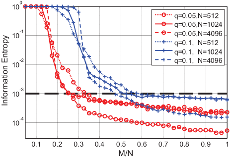
Figure 5: The entropy phase transition curve over the sampling rate $\frac{M}{N}$ for a variety of the signal length $N$ and the sparsity rate $q$ where we set the threshold $(\frac{M}{N})^{*}$ to the point achieving $\frac{1}{N}\sum\nolimits_{i=1}^{N}h(X_{i}|{\mathbf{Z}}={\mathbf{z}})\leq 10^{-3}$, which is given in Table II. These curves are information entropy of the approximate marginal posterior, $f_{\text{BP}({X_{i}})}^{(l)}(x|{\bf{Z}}={\bf{z}})$, drawn with the parameters $\sigma_{X}=5$, $x_{min}=\sigma_{X}/4$, $N_{d}=256$, $\varepsilon=10^{-5},\lambda=10^{-4}$ and a noiseless setup. In addition, we set the column weight of the matrix $\mathbf{\Phi}$ to $L=4$ for $N=512,1024$, and $L=5$ for $N=4096$, in this experiment.

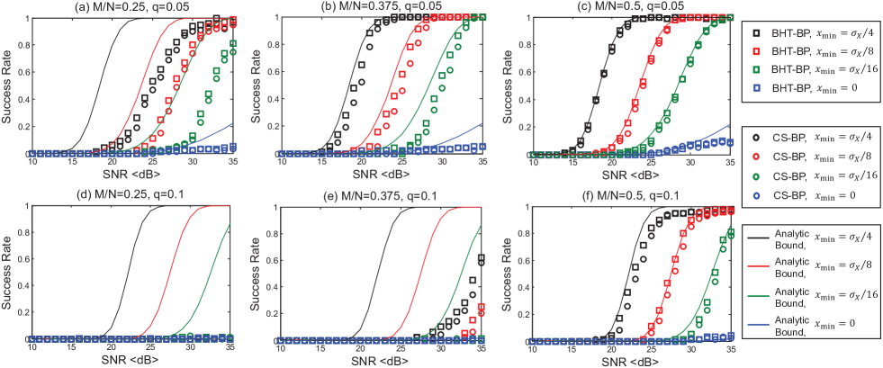
Figure 6: Experimental result for the success rate of support detection over SNR for a variety of $x_{min}$ where we consider the case of $N=1024$, $L=5$, and $\sigma_{X}=5$. In Fig.6, we plot the success rate of of BHT-BP (proposed) and CS-BP [13] together with the analytic bound for the case of $\mathbf{\Phi}=\mathbf{I}$, where the nBP part of the both algorithms is implemented with $N_{d}=256,\varepsilon=10^{-5},\lambda=10^{-4}$.

For a comparison purpose, in this validation, we include several recent Bayesian algorithms, CS-BP [13], BCS [12], and SuPrEM [16], as well as an $l_{1}$-norm based algorithm, $l_{1}$-DS [6]. We provide brief introduction to the Bayesian algorithms in Appendix I for interested readers. In this validation, BHT-BP and CS-BP use the spike-and-dented slab prior, given in (5), by applying the uniform sampling, i.e., $\mathbf{p}_{X_{i}}:=\text{Samp}\{f_{X_{i}}(x),T_{s}\}$. Worth mentioning here is that the nBP-based solvers, such as BHT-BP and CS-BP, are only compatible with such an unusual signal prior, like the spike-and-dented slab prior, which is one main advantage of the nBP solvers. For the measurement matrix $\mathbf{\Phi}$, we basically consider a LDPC-like matrix in BHT-BP, CS-BP and BCS. In case of SuPrEM, a LDF matrix is used for the measurement generation, and $l_{1}$-DS is performed with the standard Gaussian matrix as a benchmark of the CS recovery. For fair compariosn, all types of the matrices $\mathbf{\Phi}$ are equalized to have the same column energy, i.e. $\mathbb{E}\left[{\left\|{{\phi_{\text{column}}}}\right\|_{2}^{2}}\right]=L$; therefore, each entry $\phi_{ji}$ of the standard Gaussian matrix is drawn from $\mathcal{N}(\phi_{ji};0,\frac{L}{M})$. Table I summarizes all the algorithms included in this performance validation.

V-A Threshold $(\frac{M}{N})^{*}$ for BP Convergence,

We claimed the advantage of BHT-BP over CS-BP in support detection with the rate $\frac{M}{N}$ above a certain threshold $(\frac{M}{N})^{*}$ in Section III-B. Given the rate $\frac{M}{N}\geq(\frac{M}{N})^{*}$, a BP approximation of the marginal posterior $f_{\text{BP}({X_{i}})}^{(l)}(x|{\bf{Z}}={\bf{z}})$ contains sufficiently less uncertainty on the true value $x_{0,i}$. We empirically find the threshold $\left(\frac{M}{N}\right)^{*}$ in a noiseless setup using the average information entropy, $\frac{1}{N}\sum\nolimits_{i=1}^{N}h(X_{i}|{\mathbf{Z}}={\mathbf{z}})$ which measures uncertainty of $f_{\text{BP}({X_{i}})}^{(l)}(x|{\bf{Z}}={\bf{z}})$. The empirical entropy curves in Fig.5 show sharp phase transition as $\frac{M}{N}$ increases. From the result, we set the threshold to the point achieving $\frac{1}{N}\sum\nolimits_{i=1}^{N}h(X_{i}|{\mathbf{Z}}={\mathbf{z}})\leq 10^{-3}$, which is given in Table II for a variety of the signal length $N$ and the sparsity rate $q$. We also note from Fig.5 that the entropy phase transition becomes sharper as $N$ increases.

TABLE II: Empirical Threshold $(M/N)^{*}$ for the BP convergence

Sparsity rate	$N=512$	$N=1024$	$N=4096$
$q=0.05$	0.325	0.25	0.25
$q=0.1$	0.575	0.50	0.475

V-B Support Detection Performance over SNR

Fig.6 depicts an experimental comparison of the success rate, defined in (28), between BHT-BP and CS-BP over SNR for a variety of $x_{\min}$. According to the threshold $(\frac{M}{N})^{*}$ given in Table II, the BP convergence is achieved only for the cases of (a),(b),(c),(f) in Fig.6. Therefore, we confine our discussion here to such cases, claiming the advantage of BHT-BP over CS-BP in support detection.

V-B1 SNR gain by BHT support detection

The empirical results of Fig.6 validate our claim that BHT-BP has more robust support detection ability against noise, than CS-BP. Indeed, Fig.6 shows that BHT-BP enjoys a remarkable SNR gain from CS-BP in the low SNR regime. This SNR gain is from difference of the detection criterion as discussed in Section III-A. As SNR increases, the success rate of the both algorithms gradually approach to one. In the high SNR regime, BHT-BP and CS-BP do not have notable difference in the performance.

We support the advantage of BHT-BP over CS-BP with Fig.7. This figure depicts an exemplary marginal posterior, obtained from the BP part, according to two different SNR levels, SNR=10 and 30dB, where the true value of $X_{i}$ is $x_{0,i}=-4.0$; hence $s_{i}=1$.

• When SNR is sufficiently high such as the SNR=30 dB case, both of the algorithms can successfully detect the state $S_{i}$ from the posterior since the probability mass is concentrated on the true value $x_{0,i}$.

• When SNR is low such as the SNR=10 dB case, however, CS-BP may result in misdetection because the point-mass at $x=0$ is higher than the point-mass at $x_{0,i}=-4.0$ due to the additive noise, leading to $\widehat{s}_{i}=0$. In contrast, the BHT detector decides the state $S_{i}$ by incorporating all the spread mass due the noise. This is based on that the likelihoods $f_{\mathbf{Z}}(\mathbf{z}|\mathcal{H}_{s_{i}})$, which construct the hypothesis test of (10), is associated with the entire range of the $x$-axis rather than a specific point-mass. Therefore, BHT-BP can generate $\widehat{s}_{i}=1$ and success in the detection even when SNR is low.

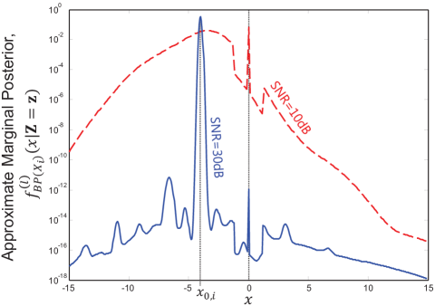
Figure 7: Example of the approximate marginal posterior $f_{\text{BP}({X_{i}})}^{(l)}(x|{\bf{Z}}={\bf{z}})$, obtained from the nBP part, for two different SNRs: 10 dB and 30 dB, where the true value of $X_{i}$ is $x_{0,i}=-4.0$, and the other parameters are set to $M/N=0.5$, $q=0.05,\sigma_{X}=5$, $l^{*}=30$, and the minimum value is $x_{min}=\sigma_{X}/4$.

V-B2 Analytic Bound of BHT detection when $\mathbf{\Phi}=\mathbf{I}$

Fig.6 includes an analytic bound of the BHT detection for the case that the measurement matrix is an identity matrix, i.e. $\mathbf{\Phi}=\mathbf{I}$, such that there is no performance degradation from lack of measurements. Therefore, this bound provides a performance benchmark of the BHT detection when $\frac{M}{N}\geq{\left({\frac{M}{N}}\right)^{*}}$, because exact marginal posteriors are given to the BHT detector under the assumption of $\mathbf{\Phi}=\mathbf{I}$. We refer to Appendix II for the detailed derivation of the analytic bound. This derivation reveals that the bound is a function of $q,x_{\min}$, and SNR. In Fig.6, it is clearly shown that the empirical points are fit into the analytic bounds as $\frac{M}{N}$ increases.

V-B3 Support detection with $x_{min}$

Fig.6 also shows the support detection behavior according to $x_{min}$, confirming that $x_{min}$ is a key parameter in the NSR problem. From Fig.6, we have the observation as given in Note 3.

Note 3 (Empirical observations for $x_{\min}$):

• All the success rate curve shift toward high SNR region as $x_{min}$ decreases.

• Extremely, when $x_{min}=0$, the experimental points stay near zero even with $\frac{M}{N}\geq{\left({\frac{M}{N}}\right)^{*}}$ and high SNR.

These empirical observations intuitively tells us that contribution of $x_{min}$ is as significant as SNR in the NSR problem, implicating that we need SNR$\to\infty$ for the perfect support recovery if the signal has $x_{min}\to 0$. Note that our interpretation on the result here shows good agreement with not only our analytic bound under the assumption of $\mathbf{\Phi}=\mathbf{I}$, but also the information-theoretical results [27],[28],[30] showing that support recovery is arbitrarily difficult by sending $x_{min}\to 0$ even as SNR becomes arbitrarily large.

V-C MSE Comparison to Recent Algorithms over SNR

In Fig.8 and Fig.9, we provide an MSE comparison among the algorithms listed in Table I and the support-aware oracle estimator over SNR for a variety of $(\frac{M}{N},q)$, where MSE^∗ denotes the performance of the support-aware oracle estimator, given as

$${\text{MSE}}^{*}:=\frac{{{\rm{Tr}}\left[{\left(\frac{1}{{\sigma_{X}^{2}}}{\bf{I}}+\frac{1}{{\sigma_{W}^{2}}}{{\bf{\Phi}}_{\mathbf{s}}^{T}{\bf{\Phi}}_{\mathbf{s}}}\right)^{-1}}\right]}}{{\mathbb{E}\left\|{{\bf{X}}}\right\|_{2}^{2}}}.$$ (31)

In this section, we discuss the comparison result by categorizing the setup of $(\frac{M}{N},q)$ into two cases: the “region of $\frac{M}{N}\geq{\left({\frac{M}{N}}\right)^{*}}$” and the “region of $\frac{M}{N}<{\left({\frac{M}{N}}\right)^{*}}$” cases, according to the empirical threshold ${\left({\frac{M}{N}}\right)^{*}}$ given in Table II, where we fix the parameters $N=1024$, $L=5$, $\sigma_{X}=5$, $x_{min}=\sigma_{X}/4$.

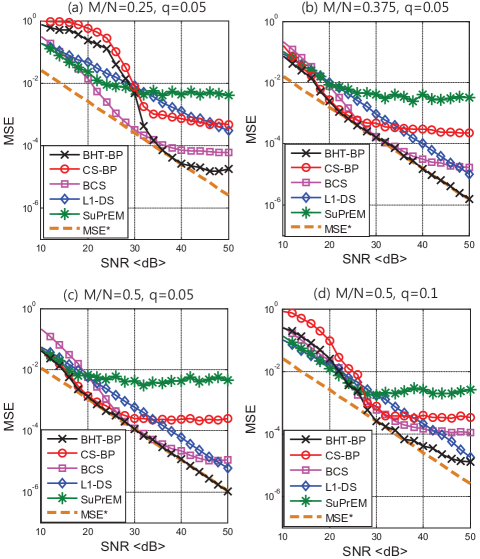
Figure 8: MSE comparison among the algorithms (BHT-BP (Proposed), CS-BP [13], SuPrEM [16], BCS [12], $l_{1}$-DS [6]) over SNR where we consider signal recovery with $\frac{M}{N}\geq{\left({\frac{M}{N}}\right)^{*}}$. We simulate the MSE performance under $N=1024$, $L=5$, $\sigma_{X}=5$, $x_{min}=\sigma_{X}/4$. The nBP part embedded in BHT-BP (proposed) and CS-BP is implemented with $N_{d}=128$ and $\varepsilon=10^{-5},\lambda=10^{-4}$.

V-C1 MSE performance in region of $\frac{M}{N}\geq{\left({\frac{M}{N}}\right)^{*}}$

With Fig.8, we argue that in the region of $\frac{M}{N}\geq{\left({\frac{M}{N}}\right)^{*}}$, BHT-BP catches up with the oracle performance, MSE^∗, beyond the SNR point allowing the accurate support finding. Fig.8-(b) and -(c) validate our claim by showing that the BHT-BP curve coincides very closely with the MSE^∗ curve beyond a certain SNR point. Worth mentioning here is that the SNR point, which starts to achieve the oracle MSE^∗, nearly corresponds to the point which attains the perfect support detection with $P_{\text{succ}}\approx 1.0$ in Fig.6. For the cases of Fig.8-(a) and -(d), the BHT-BP curve does not fit to the oracle MSE^∗ at the high SNR region. The reason is coming from lack of measurements for the BP convergence. Indeed, it is observed from Fig.5 that the entropy points corresponding to $(\frac{M}{N},q)$ of Fig.8-(a) and -(d) is in not a steady region but a transient region. This means that the corresponding posterior includes residual uncertainty on $X_{i}$. Although this residual uncertainty does not remarkably work in the low SNR region due to noise effect, it is gradually exposed as SNR increases, degrading the MSE performance in the high SNR region.

In Fig.8, the CS-BP curve forms an error floor as SNR increases, leading to a MSE gap from BHT-BP in the high SNR regime. This MSE gap is mainly caused by the quantization error of the nBP. Since CS-BP obtains its estimate directly from the sampled posteriors, the quantization error is unavoidable, leading to an error floor. The level of the floor can be approximately predicted by the MSE degradation of the quantization, given as

$$\frac{{\mathbb{E}\left\|{{Q_{{T_{s}}}}[{{\bf{X}}_{\bf{S}}}]-{{\bf{X}}_{\bf{S}}}}\right\|_{2}^{2}}}{{\mathbb{E}||{{\bf{X}}_{\bf{S}}}||_{2}^{2}}}=\frac{{T_{s}^{2}/12}}{{\sigma_{X}^{2}}}=\frac{3}{N_{d}^{2}}$$ (32)

where $Q_{T_{s}}[\cdot]$ is the quantization function with the step size $T_{s}$ given in (19), and $\mathbf{X}_{\mathbf{S}}$ is a random vector on the signal support ${\mathbf{S}}$. Under our joint detection-and-estimation structure, the LMMSE estimator (18) enables BHT-BP to go beyond the error floor.

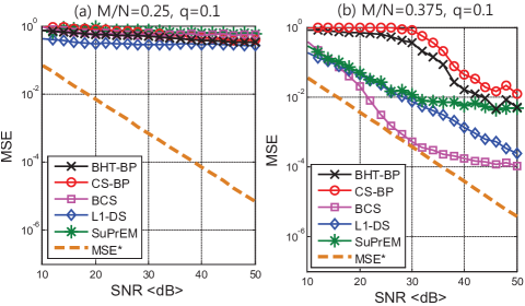
Figure 9: MSE comparison among the algorithms (BHT-BP (Proposed), CS-BP [13], SuPrEM [16], BCS [12], $l_{1}$-DS [6]) over SNR where we consider signal recovery with $\frac{M}{N}<{\left({\frac{M}{N}}\right)^{*}}$. We simulate the MSE performance under $N=1024$, $L=5$, $\sigma_{X}=5$, $x_{min}=\sigma_{X}/4$. The nBP part embedded in BHT-BP (proposed) and CS-BP is implemented with $N_{d}=128$ and $\varepsilon=10^{-5},\lambda=10^{-4}$.

For SuPrEM, the performance is poor to the other algorithms in the experimental results of Fig.8. But, it is not surprising since SuPrEM is basically for signals having fixed signal sparsity $K$. Indeed, the SuPrEM algorithm requires the sparsity $K$ as an input parameter. However, in many cases, the signal sparsity $K$ is unknown and random. In our basic setup, recall that we assumed signals having Binomial random sparsity, i.e., $K\sim\mathcal{B}(k;N,q)$. Therefore, naturally SuPrEM underperforms the other algorithms in this experiment. $l_{1}$-DS and BCS are comparable to BHT-BP, but $l_{1}$-DS has a certain SNR loss from the BHT-BP over all range of SNR, and BCS shows an error floor at high SNR region.

V-C2 MSE performance in region of $\frac{M}{N}<{\left({\frac{M}{N}}\right)^{*}}$

In Fig.9, we investigate the MSE comparison in the region of $\frac{M}{N}<{\left({\frac{M}{N}}\right)^{*}}$. Under the setup of $\frac{M}{N}=0.25,q=0.1$, every algorithm generally does not work as shown in Fig.9-(a). From the setup of $\frac{M}{N}=0.375,q=0.1$, all the algorithms begin to find signals but, BHT-BP underperforms BCS, L1-DS, and SuPrEM in this setup, as shown in Fig.9-(b). The reason is that in the region of $\frac{M}{N}<{\left({\frac{M}{N}}\right)^{*}}$, the BP does not converge properly due lack of the measurements such that probability mass on the true value $x_{0,i}$ is not dominant in the approximate marginal posteriors, as we discussed in Section III-B. From the results, we conclude that BHT-BP is not advantageous over the other algorithms excluding CS-BP when sufficient measurements is not maintained for the signal sparsity.

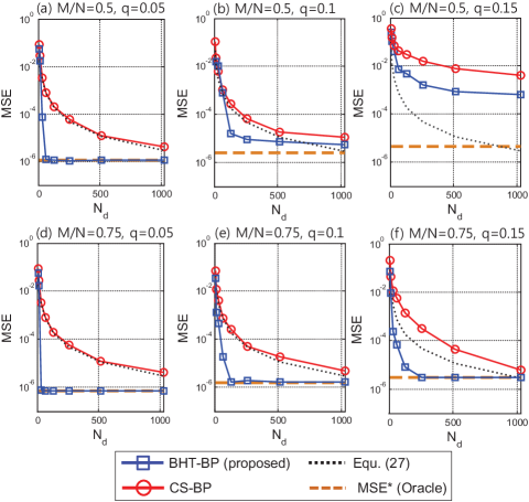
Figure 10: MSE comparison of BHT-BP (proposed) and CS-BP [13] with clean measurements (SNR=50dB) over $N_{d}\in\{8,16,32,64,128,256,512,1024\}$ for a variety of $\frac{M}{N},q$, where we plot the MSE curves together with the MSE degradation by the quantization error, given in (32). In this experiment, we consider a case of $N=1024,L=5,x_{min}=\sigma_{X}/4,\varepsilon=10^{-5},\lambda=10^{-4}$.

V-D Empirical Calibration of BHT-BP over $N_{d}$ and $L$

V-D1 Number of samples $N_{d}$ for nBP

From the discussion in Section IV-C, one can argue that the complexity of BHT-BP is highly sensitive to the number of samples $N_{d}$; therefore, BHT-BP cannot be low-computational in a certain case. It is true, but we claim that the effect of $N_{d}$ is limited in the BHT-BP recovery. To support our claim, Fig.10 compares MSE performance of BHT-BP, CS-BP, and the support-aware oracle estimator as a function of $N_{d}$ in a clean setup (SNR=50 dB) where we plot the MSE curves together with the MSE degradation by the quantization error, given in (32). From Fig.10, we confirm that BHT-BP can achieve the oracle performance if $N_{d}$ is beyond a certain level and $(\frac{M}{N},q)$ belongs to the success phase, whereas CS-BP cannot provide the oracle performance even as $N_{d}$ increases. Consequently, $N_{d}$ does not significantly contribute to the MSE of the BHT-BP recovery once $N_{d}$ exceeds a certain level. This result implies that the complexity of the BHT-BP recovery can be steady with a constant $N_{d}$ in practice. Therefore, BHT-BP can holds the low-computational property given by the BP philosophy. In addition, we confirm from Fig.10 that the MSE of CS-BP is bounded by (32).

V-D2 Column weight $L$ of LDPC-like matrices

Another interesting question is how to determine the column weight $L$ of the LDPC-like matrix $\mathbf{\Phi}$ for BHT-BP. Fig.11 provides an answer for this question by showing the MSE of the BHT-BP recovery as a function of $L$, where we consider the recovery from clean measurements (SNR= 50 dB). When $\frac{M}{N}$ is sufficiently large, for example $\frac{M}{N}=0.75$ as shown in Fig.11-(b), the BHT-BP recovery generally becomes accurate as $L$ increases. Then, the accuracy is almost constant after a certain point $L=L^{*}$. On the other hands, when $\frac{M}{N}$ is not sufficient, for example $\frac{M}{N}=0.5$ as shown in Fig.11-(a), the recovery accuracy rather can be degraded beyond a certain point $L^{*}$. The reason is that when $\frac{M}{N}$ is small, the large $L$ spoils the tree-structured property of the matrix $\mathbf{\Phi}$, reducing the accuracy of the marginal posterior approximation by BP [25],[26]. Therefore, $L$ should keep as small as possible once the desirable recovery accuracy is achieved. In the case of Fig.11, we empirically set $L^{*}=6,5$ for $\frac{M}{N}=0.5,0.75$ respectively.

From the calibration shown in Fig.10 and Fig.11, we support our claim that the computational cost of BHT-BP can be $\mathcal{O}(N\log N+KM)$ in practice by fixing $L$ and $N_{d}$, as we discussed in Section IV-C.

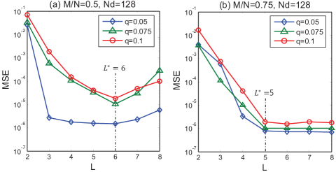
Figure 11: MSE performance of the BHT-BP recovery over the column weight $L$ of the measurement matrix $\mathbf{\Phi}$ where we set $N=1024,N_{d}=128,x_{min}=\sigma_{X}/4$, $\varepsilon=10^{-5},\lambda=10^{-4}$ and consider the recovery from clean measurements (SNR= 50dB).

VI Conclusion

The theoretical and empirical research in this paper demonstrated that BHT-BP is powerful as not only a low-computational solver, but also a noise-robust solver. In BHT-BP, we employed a joint detection-and-estimation structure consisting of the BHT support detection and the LMMSE estimation for the nonzeros on the signal support. We have shown that the BHT-BP detects the signal support based on a sequence of binary hypothesis tests, which is related to the criterion of the minimum detection error probability. This support detection approach brings SNR gain of BHT-BP from CS-BP [13], which is an existing nBP-based algorithm, for the support detection. In addition, we noted the fact that BHT-BP effectively removes the quantization error of the nBP approach in the signal recovery. We have claimed that our joint detection-and-estimation strategy prevents from degrading the MSE by the quantization error. We have supported the claim based on an empirical result that the performance of BHT-BP achieves the oracle performance when sufficient measurements is maintained for the signal sparsity. Furthermore, we confirm the impact of $x_{min}$ on the noisy sparse recovery (NSR) problem via BHT-BP. Based on the empirical evidence, we showed that exact sparse recovery with small $x_{min}$ is very demanding unless sufficiently large SNR is provided, which is an agreement with the result of [27],[28],[30] that emphasizes the importance of $x_{min}$ in the NSR problem.

Appendix I
Brief Introduction to
Recent Bayesian Algorithms

In this appendix, we provide a brief introduction to some previously proposed Bayesian algorithms for the NSR problem: BCS [12], CS-BP [13], SuPrEM [16]. These algorithms have been developed by applying several types of signal prior PDFs and statistical techniques. These algorithms are included for simulation based comparison in Section V.

VI-A BCS Algorithm

Ji et al. proposed a Bayesian algorithm based on the sparse Bayesian learning (SBL) framework, called BCS [12]. In the SBL framework, a two-layer hierarchical Gaussian model has been invoked for signal estimation. Namely, the signal prior PDF takes the form of

$${f_{\mathbf{X}}}({\bf{x}}|a,b)=\prod\limits_{i=1}^{N}{\int_{0}^{\infty}{\mathcal{N}({x}_{i};0,\gamma_{i}^{-1})}f_{\Gamma}({\gamma_{i}}|a,b)d{\gamma_{i}}},$$ (33)

where $f_{\Gamma}({\gamma_{i}}|a,b)$ is a hyper-prior following the Gamma distribution with its parameters $a,b$. Then, the MAP estimate $\widehat{\mathbf{x}}_{0}$ of the signal can be analytically expressed as a function of the hyperparameter $\mathbf{\Gamma}=[\gamma_{1},...,\gamma_{N}]$, the measurement matrix $\mathbf{\Phi}$, and the noisy measurements $\mathbf{z}$.

In BCS, the hyperparameter $\mathbf{\Gamma}$ is estimated by performing a type-II maximum likelihood (ML) procedure [11]. Specifically, the type-II ML finds the hyperparameter $\mathbf{\Gamma}$ maximizing the evidence PDF, i.e., ${f_{\mathbf{Y}}}({\mathbf{y}}|{\mathbf{\Gamma}})=\int\limits{{f_{\mathbf{Y}}}({\mathbf{y}}|{\mathbf{X}}={\mathbf{x}}){f_{\mathbf{X}}}({\mathbf{x}}|}{\mathbf{\Gamma}})\,d{\mathbf{x}}$. The expectation maximization (EM) algorithm can be an efficient approach for the type-II ML procedure. The strategy of EM is to derive a lower bound on the log evidence PDF, $\log{f_{\mathbf{Y}}}({\mathbf{y}}|{\mathbf{\Gamma}})$, at the E-step, and optimize that lower bound to find $\mathbf{\Gamma}$ at the M-step. The E-step and M-step are iterated until the lower bound becomes tighter.

The BCS algorithm is input parameter-free, which means this algorithm is adaptive to any types of signals and noise level since BCS properly catches the hyperparameter $\mathbf{\gamma}$ and the noise variance $\sigma_{W}^{2}$ during the recovery. In addition, the BCS algorithm is well compatible with any type of the measurement matrices.

VI-B CS-BP Algorithm

Baron et al. for the first time proposed the use of BP to the sparse recovery problem with LDPC-like measurement matrices [13]. The algorithm is called CS-BP. Signal model of CS-BP is a compressible signal which has a small number of large elements and a large number of near-zero elements. The authors associated this signal model with a two-state mixture Gaussian prior, given as

$${f_{\mathbf{X}}}(\mathbf{x})=\prod\limits_{i=1}^{N}{\left[q\mathcal{N}(x_{i};0,\sigma_{{X_{1}}}^{2})+(1-q)\mathcal{N}(x_{i};0,\sigma_{{X_{0}}}^{2})\right]},$$ (34)

where $q\in[0,1)$ denotes the probability that an element has the large value, and $\sigma_{X_{1}}\gg\sigma_{X_{0}}$. Therefore, the prior is fully parameterized with $\sigma_{X_{0}},\sigma_{X_{1}}$, and $q$. CS-BP performs MAP or MMSE estimation using marginal posteriors obtained from BP similarly to the proposed algorithm, where the authors applied both nBP and pBP approaches for the BP implementation. The recovery performance is not very good when measurement noise is severe since the CS-BP was basically designed to work under noiseless setup.

VI-C SuPrEM Algorithm

Most recently, Akcakaya et al. proposed SuPrEM under a framework similar to BCS which uses the two-layer hierarchical Gaussian model for the signal prior. SuPrEM was developed under the use of a specific type of hyper-prior called the Jeffreys’ prior $f_{\mathcal{J}}(\tau_{i})=1/\beta_{i},\beta_{i}\in[T_{i},\infty]\,\,\forall i\in\mathcal{V}$. This hyper-prior reduces the number of input parameters while sparsifying the signal. The overall signal prior PDF is given as

$${f_{\mathbf{X}}}({\bf{x}})=\prod\limits_{i=1}^{N}{\int_{0}^{\infty}{\mathcal{N}({x}_{i};0,\beta_{i})}f_{\mathcal{J}}({\beta_{i}})d{\beta_{i}}}.$$ (35)

SuPrEM utilizes the EM algorithm to find each hyperparameter $\beta_{i}$ like the BCS algorithm. However, differently from BCS that calculates the signal estimate $\widehat{\mathbf{x}}_{0}$ using matrix operations which include matrix inversion, SuPrEM elementwisely calculates the signal estimate from $\beta_{i}$ via a pBP algorithm. Therefore, SuPrEM can be more computationally efficient than BCS.

The measurement matrix used in SuPrEM is restricted to an LDPC-like matrix which has fixed column and row weights, called low-density-frames (LDF). They are reminiscent of the regular LDPC codes [24]. In addition, the signal model is confined to $K$-sparse signals consisting of $K$ nonzeros and $N-K$ zeros since SuPrEM includes a sparsifying step which chooses the $K$ largest elements at each end of iteration. The noise variance $\sigma_{W}^{2}$ is an optional input to the algorithm. Naturally, if the noise variance is provided, SuPrEM will produce an improved recovery performance.

Appendix II
Success Rate Analysis of the BHT Detection
when $\mathbf{\Phi}=\mathbf{I}$

Under the assumption of $\mathbf{\Phi}=\mathbf{I}$, the measurement channel can be decoupled to $N$ scalar Gaussian channels which are $Z_{j}=X_{i}+W_{j}\,\,\,\forall i,j\in\mathcal{V}$ where clearly $i=j$ holds. Accordingly, the success rate, given in (28), can be represented as the product of the complementary probability of the state error rate (SER) given in (12), i.e., ${P_{\text{succ}}}={(1-{P_{\text{SER}}})^{N}}$. Then, the problem is reduced to the analysis of the rate ${P_{\text{SER}}}$ (see Fig.4). The conditional SER given the hypothesis $\mathcal{H}_{s_{i}}$ is calculated from the likelihood PDF ${f_{{Z_{j}}}}(z|{\mathcal{H}_{{s_{i}}}})$ as following:

$${P_{{\text{SER}}|{{\mathcal{H}}_{{s_{i}}}}}}:= \Pr\{{\widehat{s}_{i}}\neq{s_{i}}|{\mathcal{H}_{{s_{i}}}}\}=\int_{{\overline{D}_{{\mathcal{H}_{{s_{i}}}}}}}{{f_{{Z_{j}}}}(z|{\mathcal{H}_{{s_{i}}}})dz},$$ (36)

where we define the decision regions with a threshold $\gamma^{\prime}$ as

$${D_{{\mathcal{H}_{0}}}}:=\{|z|<\gamma^{\prime}\}\,\,\text{and}\,\,D_{{\mathcal{H}_{1}}}:=\{|z|\geq\gamma^{\prime}\},$$ (37)

and $\overline{D}_{{\mathcal{H}_{0}}}={D_{{\mathcal{H}_{1}}}}$ vice versa. The likelihood PDFs can be obtained from

$${f_{{Z_{j}}}}(z|{\mathcal{H}_{{s_{i}}}})={\int{{{f_{Z_{j}}}(z|{X_{i}}=x)}{f_{{X_{i}}}}(x|{\mathcal{H}_{s_{i}}})dx}}$$ (38)

as we have done in (10), where ${{f_{Z_{j}}}(z|{X_{i}}=x)}=\mathcal{N}(z;x,\sigma_{W}^{2})$ under the scalar Gaussian channel. Then, the likelihood given ${\mathcal{H}_{0}}$ simply becomes ${f_{{Z_{j}}}}(z|{\mathcal{H}_{0}})=\mathcal{N}(z;0,\sigma_{W}^{2})$. In contrast, the likelihood conditioning ${\mathcal{H}_{1}}$ is not straightforward due to the dented slab part of our prior in (5), which is given by

$${f_{{Z_{j}}}}(z|{\mathcal{H}_{1}})\propto\int_{|x|\geq x_{\min}}{\mathcal{N}(z;x,\sigma_{W}^{2})\mathcal{N}(x;0,\sigma_{X}^{2})dx}$$

$$\,\,\,\,\,\,\,\,\,\,\,\,\,\,\,\,\,\,\,\,\,\,\,\,\,\,\,\,\,\,\,\,\,\,+\lambda\int_{|x|<x_{\min}}{\mathcal{N}(z;x,\sigma_{W}^{2})dx}$$

$$\,\,\,\,\,\,\,\,\,\,\,\,\,\,\,\,\,\,\,\,\,\,\,\,\,\,\,=\mathcal{N}(z;0,\sigma_{W}^{2}+\sigma_{X}^{2})$$ (39)

$$\,\,\,\,\,\,\,\,\,\,\,\,\,\,\,\,\,\,\,\,\,\,\,\,\,\,\,\,\,\,\,\,\,\,\,\times\begin{array}[]{l}\left(1-\frac{1}{2}\text{erf}\left(\frac{{A(z)}}{{\sqrt{2}}}\right)-\frac{1}{2}\text{erf}\left(\frac{{B(z)}}{{\sqrt{2}}}\right)\right)\end{array}$$ (41)

$$\,\,\,\,\,\,\,\,\,\,\,\,\,\,\,\,\,\,\,\,\,\,\,\,\,\,\,\,\,\,\,\,\,\,\,+\frac{\lambda}{2}\begin{array}[]{l}\left({{\text{erf}}\left({\frac{{{x_{{\text{min}}}}-z}}{{{\sigma_{W}}\sqrt{2}}}}\right)+\text{erf}\left({\frac{{{x_{{\text{min}}}}+z}}{{{\sigma_{W}}\sqrt{2}}}}\right)}\right)\end{array}$$ (43)

where normalization is required to satisfy $\int{f_{{Z_{j}}}}(z|{\mathcal{H}_{1}})dz=1$, and the functions $A(z),B(z)$ are respectively described as

$$A(z):=\frac{{{x_{\min}}\left(\frac{1}{{\sigma_{W}^{2}}}+\frac{1}{{\sigma_{X}^{2}}}\right)-\frac{z}{{\sigma_{W}^{2}}}}}{{\sqrt{\frac{1}{{\sigma_{W}^{2}}}+\frac{1}{{\sigma_{X}^{2}}}}}},\,\,$$

$$B(z):=\frac{{{x_{\min}}\left(\frac{1}{{\sigma_{W}^{2}}}+\frac{1}{{\sigma_{X}^{2}}}\right)+\frac{z}{{\sigma_{W}^{2}}}}}{{\sqrt{\frac{1}{{\sigma_{W}^{2}}}+\frac{1}{{\sigma_{X}^{2}}}}}}.$$

In this problem, an analytical expression of $\gamma^{\prime}$ is unattainable from the equality condition (14) since the PDF ${f_{Z_{j}}}(z|{\mathcal{H}_{1}})$ involves the error function terms as shown in (Appendix II Success Rate Analysis of the BHT Detection when $\mathbf{\Phi}=\mathbf{I}$). Therefore, we utilize a root-finding algorithm to compute $\gamma^{\prime}$. We use the SNR definition given in (30) such that ${\text{SNR = }}10{\log_{10}}\frac{{qL\sigma_{X}^{2}}}{{\sigma_{W}^{2}}}$ under the assumption of $\mathbf{\Phi}=\mathbf{I}$. We specify the decision regions (37) with $\gamma^{\prime}$, finalizing this analysis by computing the condition SERs, which are given as

$${P_{{\text{SER}}|{{\mathcal{H}}_{0}}}} ={1-{\text{erf}}\left({\frac{{{\gamma^{\prime}}}}{{{\sigma_{W}}\sqrt{2}}}}\right)},$$ (44)

$${P_{{\text{SER}}|{{\mathcal{H}}_{1}}}} =2\int_{0}^{\gamma^{\prime}}{f_{{Z_{j}}}}(z|{\mathcal{H}_{1}}){dz}$$ (45)

where the calculation of ${P_{{\text{SER}}|{{\mathcal{H}}_{1}}}}$ requires a numerical integration owing to the error function terms in ${f_{{Z_{j}}}}(z|{\mathcal{H}_{1}})$. Using (12), (44), and (45), we can evaluate the SER, then obtaining the success rate of the BHT detection when $\mathbf{\Phi}=\mathbf{I}$. We compare this analysis result to the empirical results in Section V-B.

Jaewook Kang (M’14) received the B.S. degree in information and communications engineering (2009) from Konkuk University, Seoul, Republic of Korea, and the M.S. degree in information and communications engineering (2010) from the Gwangju Institute of Science and Technology (GIST), Gwangju, Republic of Korea. He is currently pursuing the Ph.D. degree in information and communications engineering at the GIST. His research interests lie in the broad areas of compressed sensing, machine learning, wireless communications, and statistical signal processing.

Heung-No Lee (SM’13) received the B.S., M.S., and Ph.D. degrees from the University of California, Los Angeles, CA, USA, in 1993, 1994, and 1999, respectively, all in electrical engineering. From 1999 to 2002, he was with HRL Laboratories, LLC, Malibu, CA, USA, as a Research Staff Member from 1999 to 2002. From 2002 to 2008, he was with the University of Pittsburgh, Pittsburgh, PA, USA, as an Assistant Professor. He joined Gwangju Institute of Science and Technology (GIST), Korea, where he is currently a Professor. His general areas of research include information theory, signal processing, communications/networking theory, and their application to wireless communications and networking, compressive sensing, future internet, and brain- computer interface.

Kiseon Kim (SM’98) received the B.Eng. and M.Eng. degrees, in electronics engineering, from Seoul National University, Korea, in 1978 and 1980, and the Ph.D. degree in electrical engineering systems from University of Southern California, Los Angeles, in 1987. From 1988 to 1991, he was with Schlumberger, Houston, Texas. From 1991 to 1994, he was with the Superconducting Super Collider Lab, Texas. He joined Gwangju Institute of Science and Technology (GIST), Korea, in 1994, where he is currently a Professor. His current interests include wideband digital communications system design, sensor network design, analysis and implementation both, at the physical layer and at the resource management layer.

References

- [1] M. Lustig, D. L. Donoho, and J. M. Pauly, “Sparse MRI: The application of compressed sensing for rapid MR imaging,” Magnetic Resonance in Medicine, vol. 58, issue 6, pp. 1182-1195, Dec. 2007.
- [2] M. Duarte, M. Davenport, D. Takhar, J. Laska, T. Sun, K. Kelly, and R. Baraniuk, “Single-pixel imaging via compressive sampling,” IEEE Signal Processing Magazine, vol. 25, no. 2, pp. 83-91, Mar. 2008,
- [3] M. Mishali, Y. C. Eldar, O. Dounaevsky, and E. Shoshan, “Xampling: Analog to digital at sub-Nyquist rates,” IET Circuits, Devices and Systems, vol. 5, issue 1, pp. 8-20, Jan. 2011.
- [4] D. L. Donoho, M. Elad, and V. Temlyakov, “Stable recovery of sparse overcomplete representations in the presence of noise,” IEEE Trans. Inform. Theory, vol. 52, no. 1, pp. 6-18, Jan. 2006.
- [5] J. A. Tropp, “Just relax: convex programming methods for identifying sparse signals in noise,” IEEE Trans. Inform. Theory, vol. 52, no. 3, pp. 1030-1051, 2006.
- [6] E. Candes and T. Tao, “The Dantzig selector: statistical estimation when p is much larger than n,” Ann. Statist., vol. 35, no. 6, pp. 2313-2351, 2007.
- [7] R. Tibshirani, “Regression shrinkage and selection via the lasso,” J. Roy. Statisti. Soc., Ser. B, vol. 58, no. 1, pp. 267-288, 1996.
- [8] J. A. Tropp and A. C. Gilbert, “Signal recovery from random measurements via orthogonal matching pursuit,” IEEE Trans. Inform. Theory, vol. 53, no. 12, pp. 4655-4666, Dec. 2007.
- [9] D. Needell, J. Tropp, ”COSAMP: Iterative signal recovery from incomplete and inaccurate samples,” Appl. and Comput. Harmon. Anal., vol. 26, no. 3, pp. 301-321, 2008.
- [10] A. M. Bruckstein, D. L. Donoho, and M. Elad, “From sparse solutions of systems of equations to sparse modeling of signals and images,” SIAM Rev., vol. 51, no. 1, pp. 34-81, Feb. 2009.
- [11] M. E. Tipping, “Sparse Bayesian learning and the relevance vector machine,” J. Mach. Learn. Res., vol. 1, pp. 211-244, 2001.
- [12] Shihao Ji, Ya Xue, and Lawrence Carin, “Bayesian compressive sensing,” IEEE Trans. Signal Process., vol. 56, no. 6, pp. 2346-2356, June. 2008.
- [13] D. Baron, S. Sarvotham, and R. Baraniuk, “Bayesian compressive sensing via belief propagation,” IEEE Trans. Signal Process., vol. 58, no. 1, pp. 269-280, Jan. 2010.
- [14] J. Kang, H.-N. Lee, and K. Kim, “Bayesian hypothesis test for sparse support recovery using belief propagation,” Proc. of IEEE Statistical Signal Processing Workshop (SSP), pp. 45-48, Aug. 2012.
- [15] X. Tan and J. Li, “Computationally efficient sparse Bayesian learning via belief propagation,” IEEE Trans. Signal Process., vol. 58, no. 4, pp. 2010-2021, Apr. 2010.
- [16] M. Akcakaya, J. Park, and V. Tarokh, “A coding theory approach to noisy compressive sensing using low density frame,” IEEE Trans. Signal Process., vol. 59, no. 12, pp. 5369-5379, Nov. 2011.
- [17] D. L. Donoho, A. Maleki, and A. Montanari, “Message passing algorithms for compressed sensing,”, Proc. Nat. Acad. Sci., vol. 106, pp. 18914-18919, Nov. 2009.
- [18] F. R. Kschischang, B. J. Frey, and H.-A. Loeliger, “Factor graphs and the sum-product algorithm,” IEEE Trans. Inform. Theory, vol. 47, no. 2, pp. 498-519, Feb. 2001.
- [19] E. Sudderth, A. Ihler, W. Freeman, and A. S. Willsky, “Nonparametric belief propagation,” Communi. of the ACM vol 53, no. 10, pp. 95-103, Oct. 2010.
- [20] J. M. Coughlan and S. J. Ferreira, “Finding deformable shapes using loopy belief propagation,” Proc. of 12th Euro. Conf. on Comp. Vision (ECCV), pp. 453-468, 2002.
- [21] M. Isard, J. MacCormick, and K. Achan, “Continuously-adaptive discretization for message-passing algorithms,” Proc. of the Adv. in Neural Inform. Process. Sys. (NIPS), 2009.
- [22] N. Noorshams, and M. J. Wainwright, “Quantized stochastic belief propagation: efficient message-passing for continuous state spaces,” Proc. of IEEE Int. Symp. Inform. Theory (ISIT), pp. 1246-1250, July, 2012.
- [23] A. T. Ihler, J. W. Fisher, R. L. Moses, and A. S. Willsky, “Nonparametric belief propagation for self-localization of sensor networks,” IEEE Journal on Sel. Areas in Communi., vol 23, no.4, pp. 809-819, Apr. 2005.
- [24] R. G. Gallager, Low-Density Parity Check Codes, MIT Press: Cambridge, MA, 1963.
- [25] D. J. MacKay, Information theory, inference, and learning algorithms, Cambridge University Press, 2003, Available from www.inference.phy.cam.ac.uk/mackay/itila/
- [26] T. Richardson, and R. Urbanke, “The capacity of low-density parity check codes under message-passing decoding,” IEEE Trans. Inform. Theory, vol. 47, no. 2, pp. 599-618, Feb. 2001.
- [27] W. Wang, M. J. Wainwright, and K. Ramchandran, “Information-theoretic limits on sparse signal recovery: Dense versus sparse measurement matrices,” IEEE Trans. Inform. Theory, vol. 56, no. 6, pp. 2967-2979, Jun. 2010.
- [28] M. J. Wainwright, “Information-theoretic limits on sparsity recovery in the high-dimensional and noisy setting,” IEEE Trans. Inform. Theory, vol. 55, no. 12, pp. 5728-5741, Dec. 2009.
- [29] M. Akcakaya and V. Tarokh, ”Shannon-theoretic limit on noisy compressive sampling,” IEEE Trans. Inform. Theory, vol. 56, no. 1, pp. 492-504, Jan. 2010.
- [30] A. Fletcher, S. Rangan, and V. Goyal, “Necessary and sufficient conditions for sparsity pattern recovery,” IEEE Trans. Inform. Theory, vol. 55, no. 12, pp. 5758-5772, Dec. 2009.
- [31] D. Middleton and R. Esposito, “Simultaneous optimum detection and estimation of signal in noise,” IEEE Trans. Inform. Theory, vol. 14, no. 3, pp. 434-444, May. 1968.
- [32] S. Kay, Fundamentals of Statistical Signal Processing Volume I:Detection Theory, Prentice Hall PTR, 1993.
- [33] S. Kay, Fundamentals of Statistical Signal Processing Volume II:Estimation Thoery, Prentice Hall PTR, 1993.
- [34] Ake Bjorck, Numerical Methods for Least Squares Problems,,SIAM: PA, 1996.
- [35] F. Pukelsheim, “The three sigma rule,” The American Statistician, vol. 48, no. 2, May. 1994.
- [36] H. Ishwaran and J. S. Rao, “Spike and slab variable selection : Frequentist and Bayesian strategies,” Ann. Statist., vol.33, pp. 730-773, 2005.
- [37] D. Guo and S. Verdu, “Randomly spread CDMA: Asymptotics via statistical physics,” IEEE Trans. Inform. Theory, vol. 51, no. 6, pp. 1983-2010, Jun. 2005.
- [38] D. Guo and C. C. Wang, “Multiuser detection of sparsely spread CDMA,” IEEE J. Sel. Areas Comm., vol. 26, no. 3, pp. 421-431, Mar. 2008.
- [39] Frey, B. J. and D. J. MacKay, “A revolution: Belief propagation in graphs with cycles,” Proc. of the 11th Annual Conference on Neural Inform. Proces. Sys., (NIPS), pp. 479-485, Dec. 1997.
- [40] K.P. Murphy, Y. Weiss, and M.I. Jordan, “Loopy belief propagation for approximate inference: An empirical study,” Proc. of the 5th conf. on Uncertainty in artificial intelligence, Morgan Kaufmann Publishers Inc., pp. 467-475, 1999.
- [41] G. Moustakides, G. Jajamovich, A. Tajer, and X. Wang, “Joint detection and estimation: optimum tests and applications,” IEEE Trans. Inform. Theory, vol. 58, no. 7, pp. 4215-4229, June 2012.
- [42] C. M. Bishop, Pattern Recognition and Machine Learning, Springer: NY, 2006.