Dynamical System Analysis for DBI Dark Energy interacting with Dark Matter
Abstract
A dynamical system analysis related to Dirac-Born-Infeld (DBI) cosmological model has been investigated in this present work. For spatially flat FRW space time, the Einstein field equations for DBI scenario has been used to study the dynamics of DBI dark energy interacting with dark matter. The DBI dark energy model is considered as a scalar field with a non standard kinetic energy term. An interaction between the DBI dark energy and dark matter is considered through a phenomenological interaction between DBI scalar field and the dark matter fluid. The field equations are reduced to an autonomous dynamical system by a suitable redefinition of the basic variables. The potential of the DBI scalar field is assumed to be exponential. Finally, critical points are determined, their nature have been analyzed and corresponding cosmological scenario has been discussed.
Keywords: DBI dark energy , Equilibrium point, Stability.
PACS Numbers: 98.80.-k, 98.80.Jk , 95.36.+x
I Introduction
Recent cosmological observations of Type Ia Supernovae strongly indicate that the universe at present has an accelerated expansion [1, 2 ]. This has been supported by subsequent observations from Cosmic Microwave Background Radiation [CMBR][3, 4], Baryon Accoustic Oscillation [5] etc. In general, within the framework of Einstein gravity, this late time acceleration is attributed to dark energy (DE) having negative pressure . Though the nature of dark energy is still unknown, the simplest choice for dark energy is cosmological constant or vacuum energy density which fits well for wide range of astronomical data. But fine tuning and coincidence problem are significant problems associated with cosmological constant [6, 7, 8]. To alleviate these problems, scalar fields having variable equation of state are introduced . Various scalar field models of dynamical DE like quintessence [9,10,11], K-essence [12,13], Phantom [14, 15], tachyon [16, 17], dilatonic ghost condensate [18], quintom [19, 20], etc have been investigated [21] .
On the other hand, from string-theoretic point of view the early accelerated expansion (i.e inflation) can be described by Dirac-Born-Infeld (DBI) inflation [22, 23, 24]. This model is a special case of K- inflation models [25] and is characterized by the open string sector through dynamical Dp-branes. It is found that the simplest DBI models are effectively indistinguishable from the usual (field theoretic) slow-roll models of inflation . In the present work , we shall examine whether the DBI model can explain the observed late time acceleration, choosing the DBI scalar field as DE. As the density of dark matter is comparable to dark energy in the present universe, so it is reasonable to consider an interaction between the two dark components. The evolution equations are converted into an autonomous system by suitable transformation of the basic variables and a phase space analysis is done. Finally, we check for any late-time attaractor solution in the phase space. The plan of the paper is as follows : Section II deals with the basic equations related to DBI model. Autonomous system has been constructed in section III and analysis of crtical points is presented in section IV.
II Basic Equations
In a four-dimensional spatially flat Friedman-Robertson-Walker (FRW) spacetime filled with a non-cannonical scalar field of type DBI , the energy density and pressure of DBI scalar field are given by
| (1) |
and
| (2) |
where has the form of a Lorentz boost factor,
| (3) |
is the potential, is the warp factor and may be interpreted as proper velocity of the brane. We assume the customary barotropic equation of state for the dark fluid of the form , where is the barotropic index of the DBI field. Also, positivity of the potential restricts as .
In recent past, Guendelman et al [26] have constructed a unified model of DE and dark matter (DM) using a gravitating scalar field having similar non-conventional kinetic term and finds equivalent effects. Further , the scalar field has a non standard DBI like Lagrangian density and it corresponds to tachyonic scalar field by suitable restrictions on the potential.
Now considering a flat FRW metric with scale factor a(t), the field equations are
| (4) |
and
| (5) |
where and are the energy densities of dark energy and dark matter respectively and
is Hubble rate of expansion. The
Density parameters are defined as
, with the condition . At present our universe is largely dominated by dark matter and dark energy whereas all types of other matters ( i.e baryonic) are insignificant. Further dark energy has a repulsive effect while other matters are attractive. So the interaction between them is considered as weak. However, interaction models are favoured by observed data obtained from the Cosmic Microwave Background (CMB) [27] and matter distribution at large scales [28].
Hence, if the rate of creation/ annihilation between DBI scalar field and dark matter fluid be Q, we have the conservation equation as
| (6) |
and
| (7) |
where dot denotes differentiation with respect to cosmological time, are corresponding equation of state parameters for dark energy and dark matter respectively.
The generic nature of the interaction indicates a flow of energy from DE to DM while implies the reverse and is not permissible for the validity of second law of thermodynamics [29]. As there exists no fundamental theory which specifies coupling between dark energy and dark matter, so our coupling models will necessarily be phenomenological. However, one can make a comparative study between different coupling terms from physical or other natural ways. In the present work we choose the coupling term as a linear combination of the two energy densities i.e
| (8) |
and are dimensionless coupling parameters ( such that , ). H is introduced on dimensional ground and the factor 3 is due to mathematical convenience.
From (1), (4), (7) and (8) the evolution of the DBI scalar field takes the form
| (9) |
where prime denotes differentiation with respect to . Equations (4), (6) and (9) governs the dynamics of DBI dark energy scalar field , intercating with dark matter.
III Autonomous System
As the evolution equations are very complicated in form, so we shall restrict ourselves to study the cosmological evolution through qualitative analysis. For the phase space analysis, we introduce the dimensionless variables x and y [30, 31]
| (10) |
Note that the first Friedman equation in (5) shows the interrelation between the new variables x and y as
| (11) |
Using these new variables the above evolution equations can be written as following autonomous system
| (12) |
where
are assumed to be constant. and .
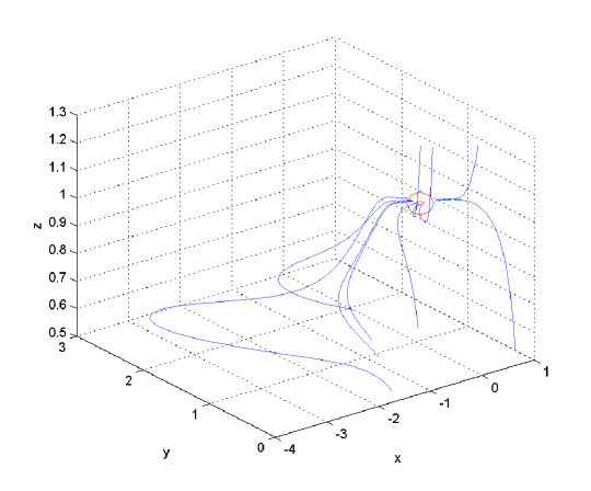
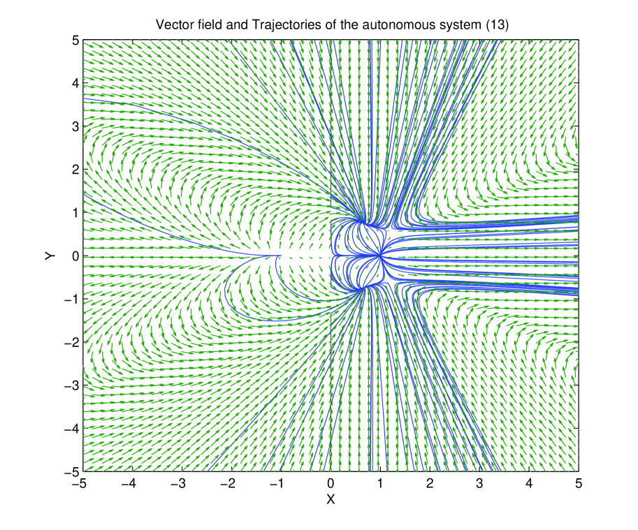
The critical points for the autonomous system (12) can be obtained by solving , and for . However , due to complicated form of the algebraic equations, it is not possible to have any analytic form of the critical points. Figure 1 depicts the phase space of the autonomous system (12) for some specific values of . From the figure 1 we see that most of the trajectories moving towards a point close to .
In particular, choosing , we have and .
the system of equations become
| (13) |
The above first order system of non-linear differential equations (13) can be considered as a 2D autonomous system. In the following section we shall study the autonomous system with some specific choice of the potential .
The equation of state for the DBI dark energy is given by
| (14) |
and the effective equation of state ( ) for DBI scalar field plus dark matter has the expression
| (15) |
with for cosmic acceleration .
It should be noted that the physical region in the phase plane is constrained by the requirement that the energy density be non-negative i.e . So from equation (11), x and y are restricted to the circular region . The equality sign indicates that there is no longer any dark matter. Further, geometrically equation (11) represents a paraboloid in -state space and it is possible to divide the 3D-state space into the following invariant sets:
A : non-vacuum 2D
no fluid matter 1D
IV Analysis of Critical points
To find the critical points of the system (13) we set
| (16) |
As is chosen to be unity so from equation (12a), the potential can be determined as
| (17) |
with , the integration constant. Using (16) , we have from (13), two non linear algebraic equations
| (18) |
| (19) |
| Equilibrium point | x | y | Nature | ||
| -1 | 0 | 0 | 1 | unstable node | |
| 0 | 0 | 1 | .27 | saddle point | |
| 1 | 0 | 0 | 1 | unstable node | |
| 0.34 | 0.94 | 0 | -0.77 | stable node | |
| 0.34 | -0.94 | 0 | -0.77 | stable node |
| Equilibrium point | x | y | Nature | ||
| -1 | 0 | 0 | 1 | unstable node | |
| 0 | 0 | 1 | 0.57 (0.77 i.e ) | saddle point | |
| 1 | 0 | 0 | 1 | unstable node | |
| 0.32 | 0.94 | 0.014 | -0.77 | stable node | |
| 0.32 | -0.94 | 0.014 | -0.77 | stable node |
| Equilibrium point | x | y | Nature | ||
| -1 | 0 | 0 | 1 | unstable node | |
| 0 | 0 | 1 | .57 | saddle point | |
| 1 | 0 | 0 | 1 | unstable node | |
| 0.66 | 0.75 | 0.002 | -0.125 | stable node | |
| 0.66 | -0.75 | 0.002 | -0.125 | stable node |
| Equilibrium point | x | y | Nature | ||
| -1 | 0 | 0 | 1 | unstable node | |
| 0 | 0 | 1 | .77 | saddle point | |
| 1 | 0 | 0 | 1 | unstable node | |
| 0.65 | 0.75 | 0.002 | -0.138 | stable node | |
| 0.65 | -0.74 | 0.002 | -0.138 | stable node |
We instantly see that (0,0) is a critical point [32, 33, 34]. For y = 0, we have with . In deriving , we have neglected the product as , .
For non zero y, the critical points are obtained as follows: is related to by the quadratic relation
| (20) |
and satisfies the cubic equation
| (21) |
with .
Note that if , then the above cubic equation in x has no real positive root , but it may have three or one negative real root. On the other hand , if , then x may have three or one positive real root but can not have any negative real root.
| Equilibrium point | x | y | Nature | ||
| -1 | 0 | 0 | 1 | unstable node | |
| 0 | 0 | 1 | .27 | saddle point | |
| 1 | 0 | 0 | 1 | unstable node | |
| 0.62 | 0.49 | .375 | 0.245 | stable spiral | |
| 0.62 | -0.49 | 0.375 | 0.245 | stable spiral |
| Equilibrium point | x | y | Nature | ||
| -1 | 0 | 0 | 1 | unstable node | |
| 0 | 0 | 1 | .57 | saddle point | |
| 1 | 0 | 0 | 1 | unstable node | |
| 0.75 | 0.44 | 0.244 | 0.51 | stable spiral | |
| 0.75 | -0.44 | 0.244 | 0.51 | stable spiral |

| Equilibrium point | x | y | Nature | ||
| -1 | 0 | 0 | 1 | unstable node | |
| 0 | 0 | 1 | .27 | saddle point | |
| 1 | 0 | 0 | 1 | unstable node | |
| -0.34 | 0.94 | 0 | -0.77 | stable node | |
| -0.34 | -0.94 | 0 | -0.77 | stable node |
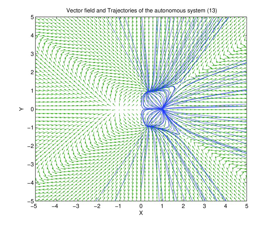
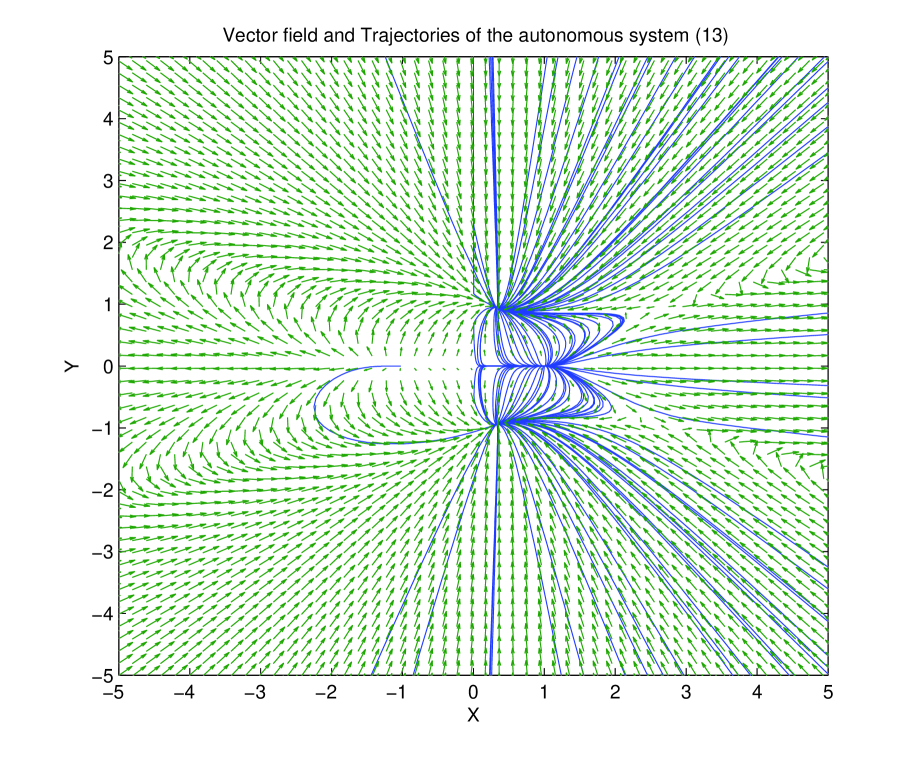
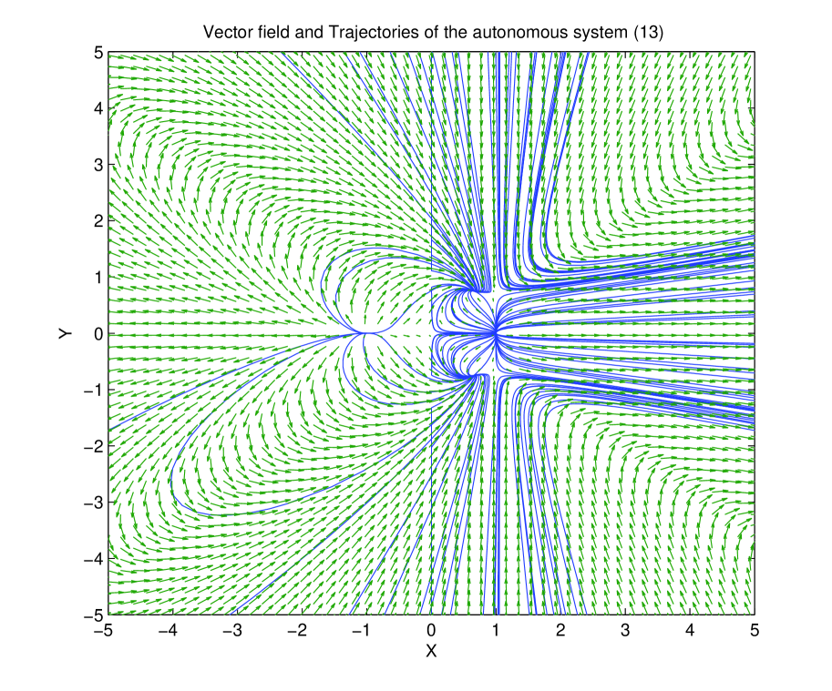
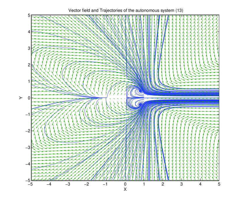
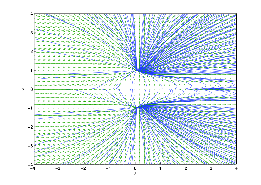
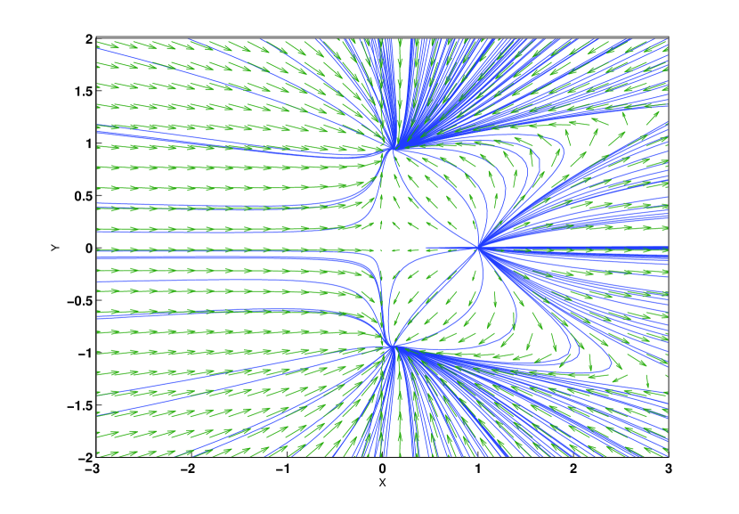
Phase portrait for the system is drawn for different values of and [ Fig 2 to Fig 7]. The Critical points for the system (13), corresponding density parameter for dark matter, effective equation of state parameter , stability are presented in tables I to VII . We have checked as expected that there is no significant change in critical points or in their stability for variation of or , but critical points and stability may vary if and change. If we keep fixed and vary no change or insignificant change in critical points is noticed. We may conclude that interaction has no significant effect on the existence as well as on the stability of the critical points. We should mention here that since the system is complicated , so the analysis is done using some numerical values of the parameters involved and by the phase space only.
For different values of , and are either unstable node or saddle point. Tables show that critical point corresponding to is saddle in nature. So in the absence of dark energy i.e when the universe is dominated by dark matter , the present DBI model can not describe the evolution of the universe.
The critical points in table I, or equivalently in table II and in table VII are interesting in present cosmological scenario. These two critical points represent late time accelerated expansion of the universe and are stable in nature being a stable node. Critical points or are completely characterized by DE (the DBI scalar field). It should be noted that these critical points describe cosmic evolution only in quintessence era. Critical points , , , , , are stable in nature but do not correspond to late time acceleration. Further, it may be noted that there does not exist any critical point corresponding to inflationary scenario in early universe.
On the other hand, to examine whether the present model can be extended to the phantom barrier (i.e ), we see from equation (15) that it is possible if . Also the points will satisfy the non-linear algebraic equations (18) and (19) provided the coupling parameter in the interaction term (8) is zero . The phase portrait corresponding these two critical points are shown in figure 8 and 9. Nature of these two critical points and corresponding physical parameters are given in tabular form in table VIII .
| Equilibrium point | x | y | Nature | ||
|---|---|---|---|---|---|
| 0 | 1 | 0 | -1 | stable node | |
| 0 | -1 | 0 | -1 | stable node |
Thus both the critical points are stable in nature and correspond to model (phantom barrier).
Therefore, We may conclude that the present interacting DBI model can explain late time acceleration only upto phantom barrier but not in phantom domain which is the possible region for DE by recent observations.
Acknowledgements.
The authors are thankful to IUCAA, Pune for warm hospitality and facilities at the library as major part of the work is done during a visit to IUCAA. The authors are also thankful to UGC-DRS programme, Department of Mathematics, Jadavpur University.V References
References
- (1) A. G. Riess et al., Astron. J. 116, 1009 (1998)
- (2) S. J. Perlmutter et al., Astrophys. J. 517, 565 (1999);
- (3) D. N. Spergel et al.(WMAP Collaboration), Astrophys. J. Suppl. Ser. 170, 377 (2007);
- (4) E. Komatsu et al (WMAP Collaboration), Astrophys. J. Suppl. Ser 180, 330 (2009)
- (5) Pereival et al , Mon. Not. R. Astr. S. 381, 1053 (2007)
- (6) S. Weinberg, Rev. Mod. Phys. 61, 1 (1989)
- (7) V. Sahni and A. Starobinsky, Int. J. Mod. Phys. D 9, 377 (2000)
- (8) S. M. Carroll, Liv. Rev. Lett. 4, 1 (2001)
- (9) B. Ratra and P. J. E. Peebles Phys. Rev. D 37, 3406 (1988)
- (10) R. R. Caldwell, R. Dave and P. J. Steinherdt, Phys. Rev. Lett 80, 1582 (1998)
- (11) I. Zlatev, L. Wang and P. J. Steinhardt, Phys. Rev. Lett. 82, 896 (1999)
- (12) C. Armendariz-Picon, V. Mukhanov and P. J. Steinhardt, Phys. Rev. Lett. 85, 4438 (2000)
- (13) C. Armendariz-Picon, V. Mukhanov and P. J. Steinhardt, Phys. Rev. D 63, 103510 (2001)
- (14) R. R. Caldwell, Phys. Lett. B 545, 23 (2002)
- (15) R. R. Caldwell, M.Kamionkowski and N. N. Weinberg, Phys. Rev. Lett. 91, 071301 (2003)
- (16) A. Sen, JHEP 0207, 065(2002)
- (17) T. Padmanabhan, Phys. Rev. D 66, 021301 (2002)
- (18) F. Piazza and S. Tsujikawa, JCAP 0407, 004 (2004)
- (19) E. Elizalde, S. Nojiri and S. D. Odintsov, Phys. Rev. D 70, 043539( 2004)
- (20) S. Nojiri and S. D. Odintsov and S. Tsujikawa, Phys. Rev. D 71, 063004(2005)
- (21) L. Amendola and S. Tsujikawa, Dark Energy: Theory and Observations (Cambridge Univ. Press, Cambridge, England, 2010)
- (22) E. Silverstein and D. Tong, Phys. Rev. D 70, 103505 (2004)
- (23) X. Chen, Phys. Rev. D 71, 063506 (2005)
- (24) Luis P. Chimento, Ruth Lazkoz, and Mart n G. Richarte, Phys. Rev. D 83, 063505 (2011)
- (25) C. Armendariz-Picon, T. Damour and V. Mukhanov , Phys. Lett. B 458, 209 (1999)
- (26) E. Guendelman, D. Singleton and N. Yongram, JCAP 11, 044 (2012)
- (27) G. Olivares, F. Atrio-Barandela and D. Pavon , Phys.Rev. D 71, 063523 (2005)
- (28) G. Olivares, F. Atrio-Barandela and D. Pavon , Phys.Rev. D 74, 043521 (2006)
- (29) D. Pavon, and B. Wang, Gen. Rel. Grav. 41, 1(2009)
- (30) E. J. Copeland, A. R. Liddle and D. Wands, Phys. Rev. D 57, 4686 (1998).
- (31) C. Kaeonikhom, D. Singleton, S. V. Sushkov and N. Yongram, Phys. Rev. D 86, 124049 (2012)
- (32) M. Hirsch and S. Smale, ” Differential Equations, Dynamical Systems and Linear Algebra ” (1974)(2nd edn, New york: Academic)
- (33) D. K. Arrowsmith and C. M. Place, ” An Introduction to Dynamical Syatems” (1990)( Cambridge Univ. Press, Cambridge)
- (34) S. Wiggins, ”Introduction to Applied Nonlinear Dynamical Systems and Chaos” (2003)( 2nd Edn. Berlin; Springer)