Imputation of truncated p-values for meta-analysis methods and its genomic application

Abstract

Microarray analysis to monitor expression activities in thousands of genes simultaneously has become routine in biomedical research during the past decade. A tremendous amount of expression profiles are generated and stored in the public domain and information integration by meta-analysis to detect differentially expressed (DE) genes has become popular to obtain increased statistical power and validated findings. Methods that aggregate transformed $p$-value evidence have been widely used in genomic settings, among which Fisher’s and Stouffer’s methods are the most popular ones. In practice, raw data and $p$-values of DE evidence are often not available in genomic studies that are to be combined. Instead, only the detected DE gene lists under a certain $p$-value threshold (e.g., DE genes with $p$-value${}<0.001$) are reported in journal publications. The truncated $p$-value information makes the aforementioned meta-analysis methods inapplicable and researchers are forced to apply a less efficient vote counting method or naïvely drop the studies with incomplete information. The purpose of this paper is to develop effective meta-analysis methods for such situations with partially censored $p$-values. We developed and compared three imputation methods—mean imputation, single random imputation and multiple imputation—for a general class of evidence aggregation methods of which Fisher’s and Stouffer’s methods are special examples. The null distribution of each method was analytically derived and subsequent inference and genomic analysis frameworks were established. Simulations were performed to investigate the type I error, power and the control of false discovery rate (FDR) for (correlated) gene expression data. The proposed methods were applied to several genomic applications in colorectal cancer, pain and liquid association analysis of major depressive disorder (MDD). The results showed that imputation methods outperformed existing naïve approaches. Mean imputation and multiple imputation methods performed the best and are recommended for future applications.

FLA

, , , , and

T2Supported in part by NIH R21MH094862.

1 Introduction and motivation

Microarray analysis to monitor expression activities in thousands of genes simultaneously has become routine in biomedical research during the past decade. The rapid development in biological high-throughput technology results in a tremendous amount of experimental data and many data sets are available from public domains such as Gene Expression Omnibus (GEO) and ArrayExpress. Since most microarray studies have relatively small sample sizes and limited statistical power, integrating information from multiple transcriptomic studies using meta-analysis techniques is becoming popular. Microarray meta-analysis usually refers to combining multiple transcriptomic studies for detecting differentially expressed (DE) genes (or candidate markers). DE gene analysis identifies genes differentially expressed across two or more conditions (e.g., cases and controls) with statistical significance and/or biological significance (e.g., fold change). Microarray meta-analysis in many situations refers to performing traditional meta-analysis techniques on each gene repeatedly and then controlling the false discovery rate (FDR) to adjust $p$-values for multiple comparison [Borovecki et al. (2005); Cardoso et al. (2007); Pirooznia, Nagarajan and Deng (2007); Segal et al. (2004)]. Fisher’s method [Fisher (1925)] was the first meta-analysis technique introduced in microarray data analysis in $2002$ [Rhodes et al. (2002)], followed by Tippett’s minimum $p$-value method in $2003$ [Moreau et al. (2003)]. Subsequently, many meta-analysis approaches have been used in this field, including extensions of existing meta-analysis techniques and novel methods to encompass the challenges presented in the genomic setting [Choi et al. (2003), Choi et al. (2007), Moerau et al. (2003), Owen (2009), Li and Tseng (2011), and see a review paper by Tseng, Ghosh and Feingold (2012)].

To combine findings from multiple research studies, one needs to know either the effect size or the $p$-value for each study. Since the differences in data structures and statistical hypotheses across multiple studies may make the direct combination of effect sizes impossible or the result suspicious, combining $p$-values from multiple studies is often more appealing. Popular $p$-value combination methods [see review and comparative papers Tseng, Ghosh and Feingold (2012) and Chang et al. (2013)] can be split into two major categories of evidence aggregation methods (including Fisher’s, Stouffer’s and logit methods) and order statistic methods [such as minimum $p$-value, maximum $p$-value and $r$th ordered $p$-value by Song and Tseng (2014)]. Evidence aggregation methods utilize summation of certain transformations of $p$-values as their test statistics to aggregate differential expression evidence across studies. Among evidence aggregation methods, Fisher’s method is the most well known, in which the test statistic is defined as $T^{\mathrm{Fisher}}=-2\sum_{k=1}^{K}\log(p_{k})$, where $K$ is the number of independent studies that are to be combined and $p_{k}$ is the $p$-value of individual study $k,1\leq k\leq K$. Under the null hypothesis of no effect size in all studies and assuming that studies are independent and models for assessing $p$-values are correctly specified, $T^{\mathrm{Fisher}}$ follows a chi-square distribution with degrees of freedom $2K$. Fisher’s method has been popular due to its simplicity and some theoretical properties, including admissibility under Gaussian assumption [Birnbaum (1954, 1955)] and asymptotically Bahadur optimality (ABO) under equal nonzero effect sizes across studies [Littel and Folk (1971, 1973)]. Some variations of Fisher’s methods were proposed by using unequal weights or a trimmed version of Fisher’s test statistic [Olkin and Saner (2001)]. Another widely used evidence aggregation method is the Stouffer’s method [Stouffer (1949)], in which the test statistic is defined as $T^{\mathrm{Stouffer}}=\sum_{k=1}^{K}\Phi^{-1}(p_{k})$, where $\Phi^{-1}(\cdot)$ is the inverse cumulative distribution function (CDF) of standard normal distribution.

In order to combine $p$-values, all $p$-values across studies should be known. In genomic applications, however, raw data and thus $p$-values are often not available and usually only a list of statistically significant DE genes ($p$-value less than a threshold) is provided in the publication [Griffith, Jones and Wiseman (2006)]. Although many journals and funding agencies have encouraged or enforced data sharing policies, the situation has only improved moderately. Many researchers are still concerned about data ownership, and researchers whose studies are sponsored by private funding are not obligated to share data in the public domain. For example, in Chan et al. (2008), publications of $23$ colorectal cancer versus normal gene expression profiling studies were collected to perform meta-analysis to identify consistently reported candidate disease-associated genes. However, only one raw data set is available from the Gene Expression Omnibus (GEO; http://www.ncbi.nlm.nih.gov/geo/, GSE3294) and most other papers only provided a list of DE genes (and their $p$-values) under a prespecified $p$-value threshold. A second motivating example comes from a microarray meta-analysis study for pain research [LaCroix-Fralish et al. (2011)], in which $19$ microarray studies of pain models were collected to detect the gene signature and patterns of pain conditions. Among the $19$ studies, only one raw data set was available on the author’s website and all the other papers reported the DE gene lists under different thresholds.

In these two motivating examples (details to be shown in Sections 4.1 and 4.2), the incomplete data forced researchers to either drop studies with incomplete $p$-values or apply the convenient vote counting method [Hedges and Olkin (1980)]. Dropping studies with incomplete information greatly reduces the statistical power and is obviously not applicable in the two motivating examples since the complete data was available in only one study. The conventional vote counting procedure is well known as flawed and low-powered [McCarley et al. (2001)]. Ioannidis et al. (2009) attempted to reproduce $18$ microarray studies published in Nature Genetics during 2005–2006. Interestingly, only two were “in principle” replicated, six “partially” replicated and ten could not be reproduced. This result illustrates well the widespread difficulty of obtaining raw data or reproducing published results in the field. Therefore, developing methods to efficiently combine studies with truncated $p$-value information is an important problem in microarray meta-analysis.

In this paper, we assume that $K=K_{1}+K_{2}$ studies are combined. In $K_{1}$ studies, the raw gene expression data matrix and sample annotations are available and the complete $p$-values $p_{gi}$ ($1\leq g\leq G$ for genes and $1\leq i\leq K_{1}$) can be reproduced for meta-analysis. For the remaining $K_{2}$ studies, either the raw data or annotation is not available. Only incomplete information of a DE gene list (under $p$-value threshold $\alpha_{i}$ for study $i$) is provided in the journal publication. In this situation, the available information is an indicator function $\mathbh{1}_{\{p_{gi}<\alpha_{i}\}}$ to represent whether the $p$-value of gene $g$ in study $i$ is smaller than $\alpha_{i}$ or not. We outline the paper structure as the following. In Section 2 a general class of evidence aggregation meta-analysis methods under a univariate scenario was investigated for the mean imputation, the single random imputation and the multiple imputation methods, respectively, in which the exact or approximate null distributions were derived under the null hypotheses and the results are shown for the Fisher and the Stouffer methods. In Section 3.1 simulations of the expression profile were performed to compare performance of different methods. Simulations were further performed in Section 3.2 using 8 major depressive disorder (MDD) and 7 prostate cancer studies where raw data were completely available and the true best performance (complete case) could be obtained. In Section 4 the proposed methods were applied to the two motivating examples. In Section 4.1 the methods were applied to $7$ colorectal cancer studies, where the raw data were available only in $3$ studies. In Section 4.2 the proposed methods were applied to $11$ microarray studies of pain conditions, where no raw data were available. In Section 4.3 we developed an unconventional application of the proposed methods to facilitate the large computational and data storage needs in a liquid association meta-analysis. Discussions and conclusions are included in Section 5 and all proofs are left in the Appendix.

2 Methods and inferences

2.1 Evidence aggregation meta-analysis methods

Here we consider a general class of univariate evidence aggregation meta-analysis methods (for gene $g$ fixed), in which the test statistics are defined as the sum of selected transformations of $p$-values for each individual study. Without loss of generality, assuming that $F_{X}(\cdot)$ is the cumulative distribution function (CDF) of a continuous random variable $X$, the test statistic $T$ is defined as

$$T=\sum_{i=1}^{K}T_{k}:=\sum_{k=1}^{K}F^{-1}_{X}(p_{k}),$$ (1)

where $p_{k}$ is the $p$-value from the $k$th study. Theoretically, $X$ can be any continuous random variable. However, in practice, $X$ is usually selected such that the test statistic $T$ follows a simple distribution. For instance, when $X\sim\chi^{2}_{2}$, it holds $T\sim\chi^{2}_{2K}$ (Fisher’s method) and $T\sim\mathrm{N}(0,K)$ holds, provided $X\sim\mathrm{N}(0,1)$ (Souffer’s method).

The hypothesis that corresponds to testing the homogeneous effect sizes of $K$ studies by evidence aggregation methods is a union-intersection test (UIT) [Roy (1953)]:

$$H_{0}\dvtx\bigcap_{k=1}^{K}\{\theta_{k}=0\}\quad\mbox{versus}\quad H_{A}\dvtx\bigcup_{k=1}^{K}\{\theta_{k}\neq 0\}.$$ (2)

In this paper, we focus on two popular special cases: [1.]

Fisher’s method [Fisher (1925)]: When $X\sim\chi^{2}_{2}$, $T_{k}=F^{-1}_{X}(p_{k})=\break-2\log(p_{k})$.

Stouffer’s method [Stouffer (1949)]: When $X\sim\mathrm{N}(0,1)$, $T_{k}=F^{-1}_{X}(p_{k})=\Phi^{-1}(p_{k})$.

Another example is the logit method [Hedges and Olkin (1985)], where $T_{k}=-\log(\frac{p_{k}}{1-p_{k}})$. But since this method is rarely used in practice, we will not examine it further in this paper. To apply the evidence aggregation meta-analysis methods mentioned above, all the $p$-values should be observed. However, in genomic applications, it often happens that $p$-values of some studies are truncated and only their ranges are reported. Two naïve methods are commonly used to overcome this situation: the vote counting method or the available-case method which only combines studies with observed $p$-values. The available-case method discards rich information contained in the studies with truncated $p$-values and, therefore, the statistical power is reduced. Hedges and Olkin (1980) showed that the power of vote counting converges to $0$ when many studies of moderate effect sizes are combined and, therefore, the vote counting method should be avoided whenever possible. In this section, three imputation methods—mean imputation, single random imputation and multiple imputation method—are proposed and investigated to combine studies with truncated $p$-values and the corresponding null distributions are derived analytically, respectively. We first define some notation.

Assume that $K$ independent studies are to be combined and $p_{1},\ldots,p_{K}$ are the corresponding $p$-values. Without loss of generality, assume that all the $p$-values are available in the first $K_{1}$ studies and only the indicator function of DE evidence is reported in the other $K_{2}$ studies.

Define a pair $(c_{i},x_{i}),i=1,\ldots,K$ for each study, in which $c_{i}$ is the “censoring” indicator satisfying

$$c_{i}:=\cases{0,&\quad$\mbox{if }p_{i}\mbox{ is observed }(\mbox{i.e.},1\leq i\leq K_{1}),$\vspace*{2pt}\cr 1,&\quad$\mbox{if }p_{i}\mbox{ is censored }(\mbox{i.e.},K_{1}+1\leq i\leq K),$}$$ (3)

and $x_{i}$ is the final observed values which is defined as

$$x_{i}:=\cases{p_{i},&\quad$\mbox{if }c_{i}=0,$\vspace*{2pt}\cr\mathbh{1}_{\{p_{i}<\alpha_{i}\}},&\quad$\mbox{if }c_{i}=1,$}$$ (4)

where $\alpha_{i}$ is the $p$-value threshold for study $i\ (K_{1}+1\leq i\leq K_{1}+K_{2}=K)$. For each $i=1,2,\ldots,K$, one can impute the missing value by $\tilde{p}_{i}$:

$$\tilde{p}_{i}=p_{i}\cdot\mathbh{1}_{\{c_{i}=0\}}+[q_{i}\cdot\mathbh{1}_{\{x_{i}=1\}}+r_{i}\cdot\mathbh{1}_{\{x_{i}=0\}}]\cdot\mathbh{1}_{\{c_{i}=1\}}$$

with $q_{i}\in(0,\alpha_{i})$, and $r_{i}\in[\alpha_{i},1)$. Sections 2.2–2.4 develop three imputation methods for selection of $q_{i}$ and $r_{i}$.

2.2 Mean imputation method

The simplest imputation method is the mean imputation method, in which $q_{i}=\frac{\alpha_{i}}{2}$ and $r_{i}=\frac{1+\alpha_{i}}{2}$. Then the test statistic $\tilde{T}$ for truncated data satisfies

$$\tilde{T} = \sum_{i=1}^{K}\tilde{T}_{i}=\sum_{i=1}^{K}F^{-1}_{X}(\tilde{p}_{i})=\sum_{i=1}^{K_{1}}F^{-1}_{X}(p_{i})+\sum_{j=1}^{K_{2}}F^{-1}_{X}(\tilde{p}_{K_{1}+j})$$

$$= A+\sum_{j=1}^{K_{2}}B_{j},$$

with

$$A = \sum_{i=1}^{K_{1}}F^{-1}_{X}(p_{i})\quad\mbox{and}$$

$$\qquad B_{j} = F^{-1}_{X}(\tilde{p}_{K_{1}+j})$$

$$= F^{-1}\biggl{(}\frac{\alpha_{K_{1}+j}}{2}\biggr{)}\cdot\mathbh{1}_{\{p_{K_{1}+j}<\alpha_{K_{1}+j}\}}$$

$${}+F^{-1}\biggl{(}\frac{1+\alpha_{K_{1}+j}}{2}\biggr{)}\cdot\mathbh{1}_{\{p_{K_{1}+j}\geq\alpha_{K_{1}+j}\}}$$

for $j=1,\ldots,K_{2}$. Recall that under the null hypothesis, the random variable $A$ satisfies $A\sim\chi^{2}_{2K_{1}}$ for the Fisher method and $A\sim\mathrm{N}(0,K_{1})$ for the Stouffer method. Obviously, $B_{j}$ follows a Bernoulli distribution.

The results can be summarized into the following theorem (proof left to Appendix B.1):

Theorem 1

For $j=1,2,\ldots,K_{2}$ and given $t$, by defining

$$b_{j} = F_{X}^{-1}\biggl{(}\frac{\alpha_{K_{1}+j}}{2}\biggr{)}-F_{X}^{-1}\biggl{(}\frac{1+\alpha_{K_{1}+j}}{2}\biggr{)}\quad\mbox{and}$$

$$c = \sum_{j=1}^{K_{2}}F_{X}^{-1}\biggl{(}\frac{1+\alpha_{K_{1}+j}}{2}\biggr{)},$$

it holds

$$\mathbb{P}(\tilde{T}\leq t)$$

$$\qquad=\sum_{(j_{1},\ldots,j_{K_{2}})\in\{0,1\}^{K_{2}}}\prod_{i=1}^{K_{2}}\alpha_{K_{1}+i}^{j_{i}}(1-\alpha_{K_{1}+i})^{1-j_{i}}F_{A}\Biggl{(}t-c-\sum_{i=1}^{K_{2}}j_{i}b_{i}\Biggr{)},$$

where $F_{A}(\cdot)$ is the CDF of $A$. Given the CDF, the expected values of test statistic $\tilde{T}$ under null distributions can be calculated as follows: [1.]

For Fisher’s method, it holds

$$\mathbb{E}(\tilde{T})=2K_{1}-2\sum_{j=1}^{K_{2}}\biggl{[}\alpha_{K_{1}+j}\log\biggl{(}\frac{\alpha_{K_{1}+j}}{2}\biggr{)}+(1-\alpha_{K_{1}+j})\log\biggl{(}\frac{1+\alpha_{K_{1}+j}}{2}\biggr{)}\biggr{]},$$

while the expectation of the original $T$ is $\mathbb{E}(T)=2K_{1}+2K_{2}=2K$.

For Stouffer’s method, it holds

$$\mathbb{E}(\tilde{T})=\sum_{j=1}^{K_{2}}\biggl{[}\alpha_{K_{1}+j}\Phi^{-1}\biggl{(}\frac{\alpha_{K_{1}+j}}{2}\biggr{)}+(1-\alpha_{K_{1}+j})\Phi^{-1}\biggl{(}\frac{1+\alpha_{K_{1}+j}}{2}\biggr{)}\biggr{]},$$

while the expectation of the original $T$ is $\mathbb{E}(T)=0$.

Note that there are $2^{K_{2}}$ terms summation in the right-hand side of equation (1), which may cause severe computing problem when $K_{2}$ is large. However, when some $\alpha_{i}$ are equal, the formula can be simplified. Without loss of generality, assume there are $r\geq 1$ different $p$-value thresholds $\{\beta_{1},\ldots,\beta_{r}\}$ such that

$$\sum_{j=1}^{K_{2}}\mathbh{1}_{\{\alpha_{K_{1}+j}=\beta_{1}\}}=n_{1},\ldots,\sum_{j=1}^{K_{2}}\mathbh{1}_{\{\alpha_{K_{1}+j}=\beta_{r}\}} = n_{r}\quad\mbox{and}$$

$$\sum_{l=1}^{r}n_{l} = K_{2},$$

then by defining $f(j;n_{l},\beta_{l}):=\frac{n_{l}!}{j!(n_{l}-j)!}\beta_{l}^{j}(1-\beta_{l})^{n_{l}-j}$ for $j=0,\ldots,n_{l}$ and $l=1,\ldots,r$, the formula can be simplified as

$$\mathbb{P}(\tilde{T}\leq t)$$

$$\qquad=\sum_{j_{1}=0}^{n_{1}}\cdots\sum_{j_{r}=0}^{n_{r}}\prod_{l=1}^{r}f(j_{l};n_{l},\beta_{l})$$ (10)

$$\hskip 68.0pt\qquad\quad{}\times F_{A}\Biggl{(}t-c-\sum_{l=1}^{r}j_{l}\biggl{(}F_{X}^{-1}\biggl{(}\frac{\beta_{l}}{2}\biggr{)}-F_{X}^{-1}\biggl{(}\frac{1+\beta_{l}}{2}\biggr{)}\biggr{)}\Biggr{)}.$$

Therefore, the summation is reduced from $2^{K_{2}}$ terms to $\prod_{l=1}^{r}(n_{l}+1)$ terms.

From the above theorem one concludes that $\tilde{T}$ is a biased estimator of the original $T$. This motivates the following two stochastic imputation methods.

2.3 Single random imputation method

It is well known that the mean imputation method will underestimate the variance of $\{p_{K_{1}+j}\}_{j=1}^{K_{2}}$ [Little and Rubin (2002)]. Furthermore, Theorem 1 indicates that the test statistic $\tilde{T}$ from the mean imputation method is a biased estimator of the original $T$. To avoid this problem, one can replace the mean by randomly simulating $q_{i}$ and $r_{i}$ from $\operatorname{Uniform}(0,\alpha_{i})$ and $\operatorname{Uniform}(\alpha_{i},1)$, respectively.

Recall that for $j=1,\ldots,K_{2}$, $B_{j}=F^{-1}_{X}(\tilde{p}_{K_{1}+j})$. The next theorem (proof left to Appendix B.2) states that $B_{j}\sim X$ holds under the null hypothesis, that is, $B_{j}$ and $X$ follow the same distribution.

Theorem 2

For $j=1,2,\ldots,K_{2}$, it holds

$$B_{j}\sim X.$$ (11)

The following corollary is a simple consequence of the above theorem. For the single random imputation method, the following facts hold for $\tilde{T}$: [1.]

For Fisher’s method, it holds $B_{j}\sim\chi^{2}_{2}$ and therefore $\tilde{T}\sim\chi^{2}_{2K}$.

For Stouffer method, it holds $B_{j}\sim\mathrm{N}(0,1)$ and therefore $\tilde{T}\sim\mathrm{N}(0,K)$.

Therefore, in this case, $\tilde{T}$ is an unbiased estimator of $T$ defined in equation (1).

2.4 Multiple imputation method

Although the single random imputation method allows the use of standard complete-data meta-analysis methods, it cannot reflect the sampling variability from one random sample. The multiple imputation method (MI) overcomes this disadvantage [Little and Rubin (2002)]. In MI, each missing value is imputed $D$ times. Therefore, $\{\tilde{T}^{l}\}_{l=1}^{D}$ is a sequence of test statistics which are defined as

$$\tilde{T}^{l}=\sum_{i=1}^{K}F_{X}^{-1}\bigl{(}\tilde{p}^{l}_{i}\bigr{)}=A+\sum_{j=1}^{K_{2}}B_{j}^{l}\qquad\mbox{for }l=1,\ldots,D$$ (12)

with

$$q^{l}_{i}\sim\operatorname{Uniform}(0,\alpha_{i})\quad\mbox{and}\quad r^{l}_{i}\sim\operatorname{Uniform}(\alpha_{i},1).$$ (13)

The test statistic is defined as $\overline{T}=\frac{1}{D}\sum_{l=1}^{D}\tilde{T}^{l}$, which satisfies

$$\overline{T} = A+\sum_{j=1}^{K_{2}}\Biggl{[}\Biggl{(}\frac{1}{D}\sum_{l=1}^{D}F^{-1}_{X}\bigl{(}q_{K_{1}+j}^{l}\bigr{)}\Biggr{)}\cdot\mathbh{1}_{\{p_{K_{1}+j}<\alpha_{K_{1}+j}\}}$$

$$\hskip 44.0pt{}+\Biggl{(}\frac{1}{D}\sum_{l=1}^{D}F^{-1}_{X}\bigl{(}r_{K_{1}+j}^{l}\bigr{)}\Biggr{)}\cdot\mathbh{1}_{\{p_{K_{1}+j}\geq\alpha_{K_{1}+j}\}}\Biggr{]}$$

$$= A+\sum_{j=1}^{K_{2}}\Biggl{[}\Biggl{(}\frac{1}{D}\sum_{l=1}^{D}W_{j}^{l}\Biggr{)}\cdot\mathbh{1}_{\{p_{K_{1}+j}<\alpha_{K_{1}+j}\}}+\Biggl{(}\frac{1}{D}\sum_{l=1}^{D}V_{j}^{l}\Biggr{)}\cdot\mathbh{1}_{\{p_{K_{1}+j}\geq\alpha_{K_{1}+j}\}}\Biggr{]}$$

$$= A+\sum_{j=1}^{K_{2}}\bigl{[}\overline{W}_{j}\cdot\mathbh{1}_{\{p_{K_{1}+j}<\alpha_{K_{1}+j}\}}+\overline{V}_{j}\cdot(1-\mathbh{1}_{\{p_{K_{1}+j}<\alpha_{K_{1}+j}\}})\bigr{]}=A+\sum_{j=1}^{K_{2}}Z_{j}.$$

Since $Z_{j}=\overline{W}_{j}$ with probability $\alpha_{K_{1}+j}$ and $Z_{j}=\overline{V}_{j}$ with probability $1-\alpha_{K_{1}+j}$, $Z_{j}$ is a mixture distribution of $\overline{W}_{j}$ and $\overline{V}_{j}$ and, therefore, $\overline{T}-A$ is a mixture distribution of $\{\overline{W}_{j},\overline{V}_{j},j=1,\ldots,K_{2}\}$.

Note that $W_{j}^{l}$ and $V_{j}^{l}$ are independent and identically distributed (i.i.d.) for fixed $j$. Denoting by $(\mu_{W_{j}},\sigma^{2}_{W_{j}}),(\mu_{V_{j}},\sigma^{2}_{V_{j}})$ the mean and variance of $W_{j}^{l}$ and $V_{j}^{l}$, respectively, then by the central limit theorem one concludes that for large enough $D>0$ it holds

$$\overline{W}_{j} = \Biggl{(}\frac{1}{D}\sum_{l=1}^{D}W_{j}^{l}\Biggr{)}\sim\mathrm{N}\biggl{(}\mu_{W_{j}},\frac{\sigma^{2}_{W_{j}}}{D}\biggr{)}\quad\mbox{and}$$

$$\overline{V}_{j} = \Biggl{(}\frac{1}{D}\sum_{l=1}^{D}V_{j}^{l}\Biggr{)}\sim\mathrm{N}\biggl{(}\mu_{V_{j}},\frac{\sigma^{2}_{V_{j}}}{D}\biggr{)}.$$

Then the following theorem holds.

Theorem 3

For $(j_{1},\ldots,j_{K_{2}})\in\{0,1\}^{K_{2}}$, by defining $U(j_{1},\ldots,j_{K_{2}})=\sum_{i=1}^{K_{2}}(j_{i}\overline{W}_{i}+(1-j_{i})\overline{V}_{i})$ which satisfies

$$U(j_{1},\ldots,j_{K_{2}})$$

(14)

$$\qquad\sim\mathrm{N}\Biggl{[}\sum_{i=1}^{K_{2}}\bigl{(}j_{i}\mu_{W_{i}}+(1-j_{i})\mu_{V_{j}}\bigr{)},\frac{1}{D}\sum_{i=1}^{K_{2}}\bigl{(}j_{i}\sigma^{2}_{W_{i}}+(1-j_{i})\sigma^{2}_{V_{j}}\bigr{)}\Biggr{]},$$

then for sufficiently large $D$, it holds approximately that

$$\mathbb{P}(\overline{T}\leq t)$$

$$\qquad=\sum_{(j_{1},\ldots,j_{K_{2}})\in\{0,1\}^{K_{2}}}\prod_{i=1}^{K_{2}}\alpha_{i}^{j_{i}}(1-\alpha_{i})^{1-j_{i}}\mathbb{P}\bigl{(}A+U(j_{1},\ldots,j_{K_{2}})\leq t\bigr{)}.$$

The detailed notation is left to Appendix C.

Similar to the mean imputation method, the formula can be simplified when some $p$-value thresholds are equal, that is,

$$\mathbb{P}(\overline{T}\leq t)=\sum_{j_{1}=0}^{n_{1}}\cdots\sum_{j_{r}=0}^{n_{r}}\prod_{l=1}^{r}f(j_{l};n_{l},\beta_{l})\mathbb{P}\bigl{(}A+U(j_{1},\ldots,j_{r})\leq t\bigr{)},$$ (16)

with $U(j_{1},\ldots,j_{r})=\sum_{l=1}^{r}(j_{l}F^{-1}_{X}(q_{l})+(n_{l}-j_{l})F^{-1}_{X}(r_{l})),q_{l}\sim\operatorname{Uniform}(0,\beta_{l})$ and $r_{l}\sim\operatorname{Uniform}(\beta_{l},1)$.

3 Simulation results

3.1 Simulated expression profiles

To evaluate performance of the proposed imputation methods in the genomic setting, we simulated expression profiles with correlated gene structure and variable effect sizes as follows:

Simulate gene correlation structure for $G=10\textup{,}000$ genes, $N=100$ samples in each study and $K=10$ studies. In each study, $4000$ of the $10\textup{,}000$ genes belong to $C=200$ independent clusters. [Step 1.]

Randomly sample gene cluster labels of $10\mbox{,}000$ genes ($C_{g}\in\{0,1,\break 2,\ldots,C\}$ and $1\leq g\leq G$), such that $C=200$ clusters each containing $20$ genes are generated [$\sum_{g}\mathbh{1}(C_{g}=c)=20,\forall 1\leq c\leq C=200$] and the remaining $6000$ genes are unclustered genes [$\sum_{g}\mathbh{1}(C_{g}=0)=6000$].

For any cluster $c(1\leq c\leq C)$ in study $k(1\leq k\leq K)$, sample $\Sigma^{\prime}_{ck}\sim W^{-1}(\Psi,60)$, where $\Psi=0.5I_{20\times 20}+0.5J_{20\times 20},W^{-1}$ denotes the inverseWishart distribution, $I$ is the identity matrix and $J$ is the matrix with all the entries being $1$. Set vector $\sigma_{ck}$ as the square roots of the diagonal elements in $\Sigma^{\prime}_{ck}$. Calculate $\Sigma_{ck}$ such that $\sigma_{ck}\Sigma_{ck}\sigma_{ck}^{T}=\Sigma^{\prime}_{gk}$.

Denote $g^{(c)}_{1},\ldots,g^{(c)}_{20}$ as the indices for genes in cluster $c$. In other words, $C_{g^{(c)}_{j}}=c$, where $1\leq c\leq 200$ and $1\leq j\leq 20$. Sample the expression of clustered genes by $(X^{\prime}_{g^{(c)}_{1}nk},\ldots,X^{\prime}_{g^{(c)}_{20}nk})^{T}\sim\mathit{MVN}(0,\Sigma_{ck})$, where $1\leq n\leq N=100$ and $1\leq k\leq K=10$. Sample the expression for unclustered genes $X^{\prime}_{gnk}\sim\mathrm{N}(0,1)$ for $1\leq n\leq N$ and $1\leq k\leq K$ if $C_{g}=0$. Simulate differential expression pattern. [Step 4.]

Sample effect sizes $\mu_{gk}$ from $\operatorname{Unif}(0.1,0.5)$ for $1\leq g\leq 1000$ as DE genes and set $\mu_{gk}=0$ for $1001\leq g\leq G$ as non-DE genes.

For the first $50$ control samples, $X_{gnk}=X^{\prime}_{gnk}\ (1\leq g\leq G,1\leq n\leq N/2=50,1\leq k\leq K)$. For cases, $Y_{gnk}=X^{\prime}_{g(n+50)k}+\mu_{gk}\ (1\leq g\leq G,1\leq n\leq N/2=50,1\leq k\leq K)$. In the simulated data sets, $K=10$ studies with $G=10\mbox{,}000$ genes simulated. Within each study, there were $\frac{N}{2}=50$ cases and $50$ controls. The first $1000$ genes were DE in all $10$ studies with effect sizes randomly simulated from a uniform distribution on $(0.1,0.5)$, respectively, and the remaining $9000$ were non-DE genes. We chose this effect size range to produce an averaged standardized effect size at $\frac{0.3}{1\cdot\sqrt{50}}=0.1414$ so that the DE analysis generates $\sim$500–600 candidate DE genes (Table 1), a commonly seen range in real applications. In each study, $200$ gene clusters existed, each containing $20$ genes. The correlation structure within each cluster was simulated from an inverse Wishart distribution.

In the simulations, we performed a two sample $t$-test for each gene in each study and then combined the $p$-values using the imputation methods proposed in this paper. For simplicity, we viewed the $p$-values from the last $5$ studies as truncated with thresholds $(\alpha_{1},\ldots,\alpha_{5})=(0.001,0.001,0.01,0.01,\break 0.05)$, respectively. In most genomic meta-analysis, researchers often use conventional permutation analysis by permuting sample labels to compute the $p$-values to preserve gene correlation structure. However, such a nonparametric approach is not applicable in our situation, since raw data are not available in some studies. In order to control the false discovery rate (FDR), we examined the Benjamini–Hochberg (B–H) method [Benjamini and Hochberg (1995)] and the Benjamini–Yekutieli (B–Y) method [Benjamini and Yekutieli (2001)] separately. The number of DE genes detected at nominal FDR rate $5\%$ were recorded and the true FDR rates were computed for each meta-analysis method by

$$\operatorname{FDR}=\frac{\sum_{g}\mathbh{1}(\mathrm{gene\ \mathit{g}\ detected\ with\ }g\geq 1001)}{\#\{\mathrm{genes\ detected}\}}.$$

In the multiple imputation method, $D=50$ was selected. Simulations were repeated for $50$ times and the mean and standard errors of numbers of DE genes controlled by B–H and B–Y methods and their true FDR are reported in Table 1. The results showed that the FDRs were controlled well for B–H correction but rather conservative for B–Y correction (the true FDR of B–Y is only $1/10$ of B–H at nominal $\operatorname{FDR}=5\%$). This is consistent with the previous observation that the B–Y adjustment tends to be over-conservative since it guards against any type of correlation structure [Benjamini and Yekutieli (2001)]. As a result, the B–H correction will be used for all applications hereafter. The simulation results showed consistently that imputation methods had higher statistical power than the available-case method, and the mean imputation and multiple imputation methods outperform the single random imputation method with similar performance. Surprisingly, the ratio of detected DE genes compared to the complete case increased from $41.6\%$ in the available case ($263.5/632.9$) to $80.4\%$ in mean imputation ($508.6/632.9$) using Fisher’s method. The improvement is even more significant using Stouffer’s method (from $41.8\%$ to $86.7\%$), while at the same time the true FDRs were controlled at a similar level for all methods. The result shows that imputation methods successfully utilize the incomplete $p$-value information to greatly recover the detection power.

Table 1: Simulation results for correlated data matrix at nominal $\operatorname{FDR}=5\%$

		Fisher		Stouffer
	Method/Mean (s.e.)	No. DE	True FDR	No. DE	True FDR
B–H	Complete cases	$632.9\ (32.5)$	$0.043\ (0.0013)$	$518.6\ (36.2)$	0.046 (0.0015)00
	Available-case	$263.5\ (37.4)$	$0.048\ (0.0076)$	$216.8\ (35.3)$	0.064 (0.022)000
	Mean imputation	$508.6\ (35.1)$	$0.046\ (0.0016)$	$449.8\ (36.2)$	0.047 (0.0022)00
	Single imputation	$408.9\ (35.7)$	$0.043\ (0.0018)$	$293.9\ (32.6)$	0.045 (0.0027)00
	Multiple imputation	$509.2\ (35.0)$	$0.045\ (0.0015)$	$463.8\ (35.7)$	0.050 (0.0019)00
B–Y	Complete cases	$354.0\ (34.4)$	$0.0041\ (0.00083)$	$261.7\ (33.9)$	0.0036 (0.00097)
	Available-case	$102.4\ (21.9)$	$0.0047\ (0.0012)$	$82.8\ (20.6)$	0.0029 (0.00096)
	Mean imputation	$234.5\ (32.1)$	$0.0037\ (0.00074)$	$203.8\ (30.8)$	0.0034 (0.00073)
	Single imputation	$164.0\ (27.3)$	$0.0057\ (0.0014)$	$113.5\ (22.3)$	0.0039 (0.0015)0
	Multiple imputation	$235.3\ (32.0)$	$0.0037\ (0.00075)$	$216.1\ (30.9)$	0.0050 (0.0010)0

We further examined the situation when gene dependence structure does not exist [i.e., steps 1–3 were skipped and $X^{\prime}_{gnk}\sim\mathrm{N}(0,1)$]. Table 2 shows the true type I error control under nominal significance level $5\%$ (i.e., true type I error $=\frac{\sum_{g=1001}^{10{\scriptsize{\textup{,}}}000}\mathbh{1}(\mathrm{gene\ \mathit{g}\ is\ detected\ at\ significance\ level\ 0.05})}{9000}$). The result shows adequate type I error control and confirms the validity of the closed form or approximated formula of different imputation methods in Section 2.

Table 2: Type I error control for independent data matrix at nominal significance level $5\%$

	Fisher	Stouffer
Complete cases	0.050 (0.00031)	0.050 (0.00037)
Available-case	0.050 (0.00035)	0.050 (0.00033)
Mean imputation	0.050 (0.00031)	0.050 (0.00033)
Single imputation	0.050 (0.00032)	0.051 (0.00032)
Multiple imputation	0.050 (0.00031)	0.051 (0.00031)

To investigate the impact of $D$ on the performance of the multiple imputation method, simulations were performed for $D\in\{20,30,50,100,150,200,\break 250,300,500\}$. The result is shown in Appendix A, Figure 3, which demonstrates that the performance of the multiple imputation method is quite robust for different number of imputation $D$. We use $D=50$ throughout this paper.

3.2 Simulation from complete real data sets

In this subsection the proposed methods were applied to two real microarray data sets, including $7$ prostate cancer studies [Gorlov et al. (2009)] and $8$ major depressive disorder (MDD) studies [Wang et al. (2012)]. The details are summarized in Supplement Table $1$ [Tang et al. (2014)]. For each data set, about half of the studies (four for MDD and three for prostate cancer) were randomly selected with $p$-value truncation threshold $0.05$. Five methods including complete data, available-case, single random imputation, mean imputation and multiple imputation methods were applied to the data sets with the simulated incomplete data to impute by Stouffer’s and Fisher’s methods, respectively. The generated $p$-values were corrected by the B–H method and the simulation was repeated for $50$ times. Figure 1 shows boxplots of the numbers of differentially expressed (DE) genes at $\operatorname{FDR}=1\%$ for different methods in MDD and $\operatorname{FDR}=0.5\%$ for prostate cancer data. Figure 1 indicates similar conclusions that the multiple imputation and the mean imputation methods detect more DE genes than the available-case method and single random imputation method. In the MDD example, very few DE genes (average of $16$ and $83$ for Fisher and Stouffer, resp.) were detected using the available-case method if half of the studies have truncated $p$-values. The mean and multiple imputation methods greatly improved the detection sensitivity. About $95.2\%$ (Fisher) and $96.3\%$ (Stouffer) of DE genes detected by the mean imputation method overlapped with DE genes detected by complete data analysis in MDD and about $94.7\%$ (Fisher) and $88.1\%$ (Stouffer) of DE genes detected by the mean imputation method overlapped with DE genes detected by complete data analysis in prostate cancer, showing the ability of imputation methods to recover DE gene detection power.

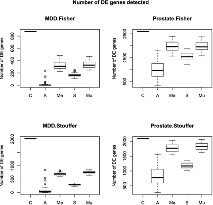
Figure 1: Number of DE genes detected by Fisher’s or Stouffer’s method. C: complete data; A: available-case; Me: mean-imputation; S: single-imputation; Mu: multiple imputation.

4 Applications

4.1 Application to colorectal cancer

In the first motivating example, we followed Chan et al. (2008) and attempted to collect 23 colorectal cancer versus normal gene expression profiling studies. Raw data were available in only one study [Bianchini et al. (2006)] and $4$ of the other $22$ studies containing more than $100$ DE genes at different $p$-value thresholds were included in our analysis. We searched the GEO database and identified two additional new studies [Jiang et al. (2008) and Bellot et al. (2012)]. The seven studies under analysis were summarized in Table 3. After gene-matching, $6361$ genes overlapped in all three studies with raw data. The available-case method, the mean imputation method, the single random imputation method and the multiple imputation method were applied for the seven studies for the Fisher and Stouffer methods, respectively, and the results were reported in Table 4. For the single random imputation method and the multiple imputation method, the analyses were repeated $50$ times and the mean and standard error of the number of DE genes detected were reported under FDR control by the B–H method. The results demonstrate that for various FDR thresholds, the mean imputation method and the multiple imputation method detected more DE genes than the available-case method and the single random imputation method, which was consistent with previous findings in simulations. Under $\operatorname{FDR}=0.01\%$ control, the Fisher and Stouffer mean imputation detected $2.07$ ($1183/571$) and $10.35$ ($383/37$) times of DE genes than those by the available-case method, respectively.

Table 3: Seven colorectal cancer versus normal tissue expression profiling studies included in analysis

	No. of	No. of	Raw data	No. of DE	No. of overlapped	$\bolds{p}$-value
Study	samples	genes	availability	genes	DE genes	threshold
Bianchini$\_2006$	024	0.7403	GSE3294	–	–	–
Bellot$\_2012$	017	18,191	GSE24993	–	–	–
Jiang$\_2008$	048	18,197	GSE10950	–	–	–
Grade$\_2007$	103	21,543	–	1950	635	1e–7
Croner$\_2005$	033	22,283	–	0130	047	0.006
Kim$\_2004$	032	18,861	–	0448	143	0.001
Bertucci$\_2004$	050	0.8074	–	0245	097	0.009

Table 4: Summary of results for colorectal cancer

	Fisher				Stouffer
FDR	Available	Mean	Single	Multiple	Available	Mean	Single	Multiple
$1\%$	2587	2855	2172.4 (2.90)	2785.4 (2.93)	1318	1675	668.4 (3.96)	1616.0 (2.10)
$0.1\%$	1472	1874	1265.6 (2.34)	1805.7 (1.50)	0299	0709	252.7 (1.93)	0680.5 (1.12)
$0.01\%$	0571	1183	0748.4 (1.89)	1138.6 (2.00)	0037	0383	102.5 (1.65)	0366.7 (0.69)

4.2 Application to pain research

The second motivating example comes from the meta-analysis of $20$ microarray studies of pain to detect the patterns of pain [LaCroix-Fralish et al. (2011)]. The original meta-analysis utilized DE gene lists from each study under different threshold criteria from $p$-value, FDR or fold change and identified $79$ “statistically significant” genes that appeared in the DE gene lists of four or more studies. The vote counting method essentially lost a tremendous amount of information with flawed statistical inference. When we attempted to repeat the meta-analysis, raw data of only one of the $20$ studies (Barr$\_2005$) could be found. The old platform used in that study, however, contained only $792$ genes and had to be excluded from further meta-analysis. In the remaining $19$ studies, $11$ studies contained DE gene lists under various $p$-value thresholds (marked bold in Supplement Table 2 [Tang et al. (2014)]) and were included in our application. In other words, this example contained exclusively only studies with truncated $p$-values. Table 5 shows the results of three imputation methods. Fisher and Stouffer identified 280 and 45 genes under $5\%$ FDR control, respectively. Note that the original meta-analysis tested the 79 genes using an overall binomial test and the statistical significance was controlled at an overall $p$-value level, not at a gene-specific FDR level. As a result, DE gene lists from the new imputation methods are theoretically more powerful and accurate.

To validate the finding, we used the Gene Functional Annotation tool from the DAVID Bioinformatics Resources website (http://david.abcc.ncifcrf.gov). DAVID applied a modified Fisher’s exact test to evaluate the association between the DE gene lists and pathways. Functional annotation of the 280 DE genes from the Fisher’s mean imputation method identified 208 pathways at $\operatorname{FDR}=5\%$, among which selected important pain-related pathways were grouped into five major biological categories and displayed in Table 6. In contrast, the 79 genes from vote counting identified only 14 pathways, of which the expected pain-related pathways under the categories of inflammation and of differentiation, development and projection are missing (see Table 6). The pathway enrichment $q$-values after multiple comparison control of the “280 gene list” were very significant, while those of the “79 gene list” were not. Since the $p$-value calculation from Fisher’s exact test can be impacted by the DE gene size, we further compared the enrichment odd-ratios of genes in the pathway versus in the DE gene list. Still the enrichment odds-ratios of the “280 gene list” were generally much higher than those for the “79 gene list,” showing stronger pain functional association from the Fisher’s mean imputation method.

Table 5: Summary of results for patterns of pain

	Fisher	Stouffer
Mean	280	45
Single	57.04 (1.6228)	16.44 (0.8605)
Multiple	280.36 (0.8105)	77.56 (0.6616)

Table 6: Summary of pathway analysis by DAVID

		280 DE			79 DE
		(Fisher’s mean imputation)			(Vote counting)
				odds			odds
Category	Pathway ID	$\bolds{p}$-value	$\bolds{q}$-value	ratio	$\bolds{p}$-value	$\bolds{q}$-value	ratio
Differentiation,	$\textbf{GO}:0030182\sim$ neuron differentiation	5.6e–6	0.0006	$3.1$	0.26	$0.95$	$1.6$
development and	$\textbf{GO}:0045664\sim$ regulation of neuron differentiation	1.6e–5	0.0011	$4.7$	0.37	$0.98$	$1.9$
projection	$\textbf{GO}:0048666\sim$ neuron development	2.5e–6	0.0003	$3.6$	0.24	$0.94$	$1.7$
	$\textbf{GO}:0051960\sim$ regulation of nervous system development	6.5e–6	0.0006	$4.2$	0.29	$0.96$	$1.9$
	$\textbf{GO}:0031175\sim$ neuron projection development	1.6e–5	0.0012	$3.7$	0.27	$0.96$	$1.8$
	$\textbf{GO}:0042995\sim$ cell projection	3.6e–11	3.2e–9	$3.5$	0.033	$0.47$	$1.9$
	$\textbf{GO}:0043005\sim$ neuron projection	3.0e–11	3.4e–9	$4.3$	0.043	$0.51$	$2.0$
	$\textbf{GO}:0030030\sim$ cell projection organization	1.6e–5	0.0012	$3.3$	0.24	$0.94$	$1.7$
Response	$\textbf{GO}:0009611\sim$ response to wounding	3.8e–10	2.8e–7	$4.3$	2.7e–5	$0.016$	$3.6$
to stimuli	$\textbf{GO}:0009719\sim$ response to endogenous stimulus	3.2e–8	1.7e–5	$3.4$	0.35	$0.97$	$1.3$
	$\textbf{GO}:0048584\sim$ positive regulation of response to stimulus	7.9e–8	2.5e–5	$4.9$	0.0049	$0.34$	$3.6$
	$\textbf{GO}:0032101\sim$ regulation of response to external stimulus	1.1e–5	0.001	$4.8$	0.043	$0.71$	$2.8$
Immune	$\textbf{GO}:0050778\sim$ positive regulation of immune response	4.2e–7	7.6e–5	$5.9$	0.018	$0.57$	$4.0$
	$\textbf{GO}:0002684\sim$ positive regulation of immune system process	1.9e–6	0.0003	$4.4$	0.0009	$0.13$	$4.2$
	$\textbf{GO}:0006956\sim$ complement activation	3.0e–5	0.0016	$11.5$	0.011	$0.46$	$8.4$
	$\textbf{GO}:0002478\sim$ antigen processing and presentation	1.3e–6	0.00022	$19.0$	0.00098	$0.12$	$10.64$
	of exogenous peptide antigen
Inflammation	$\textbf{GO}:0002673\sim$ regulation of acute inflammatory response	1.4e–6	0.0002	$14.1$	0.19	$0.93$	$3.8$
	$\textbf{GO}:0002526\sim$ acute inflammatory response	7.1e–6	0.0007	$6.7$	0.012	$0.48$	$4.4$
	$\textbf{GO}:0050727\sim$ regulation of inflammatory response	1.9e–5	0.0012	$6.9$	0.17	$0.92$	$2.8$
	$\textbf{GO}:0006954\sim$ inflammatory response	1.5e–5	0.0012	$4.1$	0.001	$0.11$	$3.8$
Regulation of	$\textbf{GO}:0051969\sim$ regulation of transmission of nerve impulse	6.0e–6	0.0006	$4.8$	0.057	$0.80$	$2.4$
Transmission

4.3 Application to a three-way association method (liquid association)

So far the proposed imputation methods were applied successfully to two real microarray data sets of colorectal cancer and pain research in which the actual $p$-values of some genes were not reported in a subset of studies. In this section we show that the proposed imputation methods can be useful in the meta-analysis of “big data” such as GWAS or eQTL, where the main computational problem is often the data storage.

In the literature it has long been argued that positively correlated expression profiles are likely to encode functionally related proteins. Liquid association (LA) analysis [Li (2002)] is an advanced three-way co-expression analysis beyond the traditional pairwise correlations. For any triplet of genes $X,Y$ and $Z$, the LA score $\mathit{LA}(X,Y|Z)$ measures the effect that expression of $Z$ to control on and off of the co-expression between $X$ and $Y$. For example, high expression of Z turns on positive correlation between $X$ and $Y$, while when expression of $Z$ is low, $X$ and $Y$ are negatively or noncorrelated. Theory in Li (2002) simplified calculation of the LA score to a linear order of sample size and made the genome-wide computation barely feasible. Supposing we want to combine $K$ studies of the liquid association, liquid association $p$-values of all triplets in all $K=10$ studies have to be stored for meta-analysis. When the number of genes $G=1000$, the number of $p$-values to be stored is $G\cdot C^{G-1}_{2}\cdot K=4.985$ GB. For a reasonable $G=20\mbox{,}000$ genome-wide analysis, storage size for all $p$-values quickly increases to $39.994$ TB. One may argue that univariate (i.e., triplet by triplet) meta-analysis may be applied repeatedly to avoid the need of storing all $p$-value results. There are many other genomic meta-analysis situations when this may not be feasible. For example, in GWAS meta-analysis under a consortium collaboration, raw genotyping data cannot be shared for privacy reasons and only the derived statistics or $p$-values can be transferred for meta-analysis. Below we describe how imputation methods can help circumvent the tremendous data storage problem.

We performed a small scale of analysis on $566$ DE genes previously reported from the meta-analysis of the eight MDD studies used in Section 3.2 [Wang et al. (2012)]. The total number of possible triplets $(X,Y|Z)$ was $90\mbox{,}180\mbox{,}780$. By setting up a $p$-value threshold at $0.001$, we only needed to store exact $p$-values for $2\mbox{,}094\mbox{,}123$ ($\sim$2.32%) triplets and the remaining were truncated as considered in this paper. Since we also needed to store the truncation index information, we only needed to store $2\times 2.32\%=4.64\%$ of the information and the compression ratio was $95.36\%$. To investigate the loss of information by the truncation, Figure 2 shows meta-analysis $p$-values [at $-\log(p)$ scale] from Fisher’s method using full data and the Fisher mean imputation method using truncated data. The result shows high concordance in the top significant triplets, which are the major targets of this exploratory analysis. Among the top $1000$ triplets detected by Fisher’s method using complete $p$-value information, $83.7\%$ of them were also identified by the top $1000$ by Fisher mean imputation. The remaining $163$ triplets were still in top ranks (rank between $1199$ and $4763$) using truncated data in the result of Fisher mean imputation. This result suggests a good potential of applying data truncation to preserve the most informative information and performing imputation to approximate the finding of the top targets when meta-analysis of “big data” is needed. The compression ratio may further increase by a more stringent truncation threshold, but the performance may somewhat decline as a trade-off.

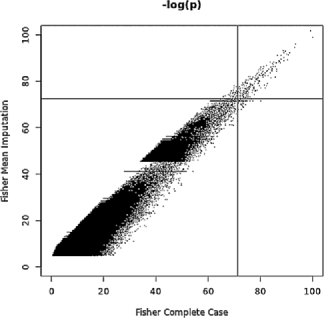
Figure 2: $-\log(p)$ comparison of the mean imputation method using truncated data with the complete case method using complete data. Vertical line: $x=71.3$. Horizontal line: $y=72.58$. Points right to vertical line are top $1000$ triplets detected by Fisher’s complete case method, and points above to horizontal line are top $1000$ triplets detected by Fisher’s mean imputation method.

5 Discussion and conclusion

When combining multiple genomic studies by $p$-value combination methods, the raw data are often not available and only the ranges of $p$-values are reported for some studies in genomic applications. This is especially true for microarray meta-analysis since owners of many microarray studies tend not to publish their data in the public domain. This incomplete data issue is often encountered when one attempts to perform a large-scale microarray meta-analysis. If raw data are not available, two naïve methods—vote counting method and available-case method—are commonly used. Since these two methods completely or largely neglect the information contained in the truncated $p$-values, their statistical power is generally low. In this paper, we proposed three imputation methods for a general class of evidence aggregation meta-analysis methods to combine independent studies with truncated $p$-values: mean imputation, single random imputation and multiple imputation methods. For each proposed imputation method, the null distribution was derived analytically for the Fisher and Stouffer methods. Theoretical results showed that the test statistics from the single random imputation and the multiple imputation methods were unbiased, while those for mean imputation methods were biased. Simulations were performed for the imputed Fisher method and imputed Stouffer method. The simulation results showed that type I errors were well controlled for all methods, which was consistent with our theoretical derivation. Compared to the naive available-case method, all the imputation methods achieved higher statistical powers, and the mean imputation and the multiple imputation methods recovered much of the power that the complete cases method achieved even when half of the studies had truncated $p$-values. Furthermore, Figure 3 in Appendix A showed that the power of the multiple imputation method was robust to the number of imputation $D$. Although small to moderate $D$ provided good results, we recommend choosing $D$ being larger than $50$ to guarantee that the central limit theorem can approximate well. Applications to two motivating examples in colorectal cancer and pain conditions showed that both mean imputation and multiple imputation performed among the best in terms of detection sensitivity and biological validation by pathway analysis.

In regression-type missing-data imputation methods, the null distribution of the error term is unknown and is assumed to be normally distributed with equal variance, a setting in which the multiple imputation method usually outperforms the mean imputation in practice and in theory [Little and Rubin (2002)], particularly because mean imputation underestimates the true variance. However, our simulation results demonstrated that the power of the two methods were quite similar. Two reasons may contribute to this result. First, although the test statistic from the mean imputation method is biased and neglects the variation of truncated $p$-values, its $p$-value can be computed accurately when the null distribution is derived analytically. Second and more importantly, we find that the test statistic of mean imputation is in fact $F^{-1}_{X}(\mathbb{E}(p))$, while for sufficiently large $D$, the test statistic of multiple imputation converges to $\mathbb{E}(F^{-1}_{X}(p))$ in distribution. It is easy to show that these two quantities are very close to each other for a small range of $p$, provided $F^{-1}_{X}(\cdot)$ is smooth. Since $F^{-1}_{X}(\cdot)$ is infinitely differentiable for the Fisher and Stouffer methods, and the small $p$-value range in $(0,\alpha)$ is particularly of interest to us, it is not surprising that the mean imputation method and multiple imputation method perform similarly. Since the mean imputation method achieved almost the same power as the multiple imputation method with less computational complexity, it is more appealing and is recommended for microarray meta-analysis, where the imputed meta-analysis method is performed repeatedly for thousands of genes. In this paper only the evidence aggregation meta-analysis methods are investigated and further work will be needed to extend these results to order statistic based methods such as minP and maxP.

Note that although the truncated $p$-value issue discussed in this paper may appear similar to the problem of “publication bias,” it is fundamentally different. Publication bias refers to the fact that a study with a large positive treatment effect is more likely to be published than a study with a relatively small treatment effect, resulting in bias if one only considers published studies. Denote by $p_{1},p_{2},\ldots,p_{N}$ the $p$-values of all conducted studies that should have been collected. Only a subset of likely more significant $p$-values $p_{1},p_{2},\ldots,p_{n}$ are observed. Under this setting, $N$ is unknown and $p_{n+1},\ldots,p_{N}$ are unknown as well. Since the number of missing publications is unknown, Duval and Tweedie proposed the “Trim and Fill” method to identify and correct for funnel plot asymmetry arising from publication bias [Duval and Tweedie (2000a) and (2000b)], in which an estimate of the number of missing studies is provided and an adjusted treatment effect is estimated by performing a meta-analysis including the imputed studies. For the truncated $p$-value problem we consider here, the total number of studies, the number of studies with truncated $p$-values and the $p$-value truncation thresholds are all known. Therefore, investigation of the imputation of truncated $p$-values in meta-analysis is different from the traditional “publication bias” problem and has not been studied in the meta-analysis literature, to the best of our knowledge.

In this paper the methods we developed mainly target on microarray meta-analysis, but the issue can happen frequently in other types of genomic meta-analysis [e.g., GWAS; Begurn et al. (2012)]. In Section 4.3 we demonstrated an unconventional application of our methods to meta-analysis of liquid association. Due to the large number of triplets tested in the three-way association, the needed $p$-value storage is huge. By preserving only the most informative data by truncation, the storage burden is greatly alleviated and our imputation methods help approximate and recover the top meta-analysis targets with little power loss. In an ongoing project, we also attempt to combine multiple genome-wide eQTL results via meta-analysis. In eQTL, regression analysis is used to investigate the association of a SNP genotyping and a gene expression. It is impractical to store all genome-wide eQTL $p$-values, as the storage space required is too large ($25\mbox{,}000$ genes $\times$ $2\mbox{,}000\mbox{,}000$ SNPS $=5\times 10^{10}$ $p$-values). A practical solution is to record only the eQTL $p$-values smaller than a threshold (say, $10^{-4}$) for meta-analysis, which leads to the same statistical setting as discussed in this paper. In another project we combine results from multiple ChIP-seq peak calling algorithms to develop a meta-caller. Since each peak caller algorithm can only report the top peaks with $p$-values smaller than a certain $p$-value threshold, we again encounter the same truncated $p$-value problem in meta-analysis. As more and more complex genomic data are generated and the need for meta-analysis increases, we expect the imputation methods we propose in this paper will find even more applications in the future.

Appendix A Supplementary figure

Fig. 3.   Power analysis at significance level $0.05$ for different numbers of imputation $D$. The dashed lines represent the theoretical asymptotic power obtained by setting $D=1000$.

Appendix B Proofs of theorems

B.1 Proof for Theorem 1

Note that in this case, for $j=K_{1}+1,\ldots,K$, it holds

$$B_{j}=F_{X}^{-1}\biggl{(}\frac{\alpha_{j}}{2}\biggr{)}\cdot\mathbh{1}_{\{p_{i}<\alpha_{j}\}}+F_{X}^{-1}\biggl{(}\frac{1+\alpha_{j}}{2}\biggr{)}\cdot\mathbh{1}_{\{p_{i}\geq\alpha_{j}\}}.$$ (17)

Let $Y_{j}\sim\operatorname{Bernoulli}(\alpha_{j})$. Since $p_{i}\sim\operatorname{Uniform}(0,1)$ under the null hypothesis, it holds

$$B_{j} = \biggl{[}F_{X}^{-1}\biggl{(}\frac{\alpha_{j}}{2}\biggr{)}-F_{X}^{-1}\biggl{(}\frac{1+\alpha_{j}}{2}\biggr{)}\biggr{]}Y_{j}+F_{X}^{-1}\biggl{(}\frac{1+\alpha_{j}}{2}\biggr{)}$$

$$= b_{j}Y_{j}+c_{j}$$

and, therefore,

$$\tilde{T}=A+\sum_{j=1}^{K_{2}}b_{j}Y_{j}+c\qquad\mbox{with }c=\sum_{j=1}^{K_{2}}c_{j}.$$ (19)

For given $t$, it holds

$$\mathbb{P}(\tilde{T}\leq t) = \mathbb{P}\Biggl{(}A+\sum_{i=1}^{K_{2}}b_{i}Y_{i}+c\leq t\Biggr{)}$$

$$= \sum_{(j_{1},\ldots,j_{K_{2}})\in\{0,1\}^{K_{2}}}\mathbb{P}\Biggl{(}A+\sum_{i=1}^{K_{2}}b_{i}Y_{i}+c\leq t|Y_{1}=j_{1},\ldots,Y_{K_{2}}=j_{K_{2}}\Biggr{)}$$

$$\hskip 70.0pt{}\times\mathbb{P}(Y_{1}=j_{1},\ldots,Y_{K_{2}}=j_{K_{2}})$$

$$= \sum_{(j_{1},\ldots,j_{K_{2}})\in\{0,1\}^{K_{2}}}\prod_{i=1}^{K_{2}}\alpha_{i}^{j_{i}}(1-\alpha_{i})^{1-j_{i}}\mathbb{P}\Biggl{(}A\leq t-c-\sum_{i=1}^{K_{2}}j_{i}b_{i}\Biggr{)}$$

$$= \sum_{(j_{1},\ldots,j_{K_{2}})\in\{0,1\}^{K_{2}}}\prod_{i=1}^{K_{2}}\alpha_{i}^{j_{i}}(1-\alpha_{i})^{1-j_{i}}F_{A}\Biggl{(}t-c-\sum_{i=1}^{K_{2}}j_{i}b_{i}\Biggr{)},$$

where $F_{A}(\cdot)$ is the CDF of $A$.

B.2 Proof for Theorem 2

We show that for given $t$

$$\mathbb{P}(B_{i}\leq t)$$

$$\qquad=\mathbb{P}\bigl{(}F^{-1}_{X}(\tilde{p}_{i})\leq t\bigr{)}=\mathbb{P}\bigl{(}\tilde{p}_{i}\leq F_{X}(t)\bigr{)}$$

$$\qquad=\mathbb{P}(x_{i}=1)\cdot\mathbb{P}\bigl{(}\tilde{p}_{i}\leq F_{X}(t)|x_{i}=1\bigr{)}+\mathbb{P}(x_{i}=0)\cdot\mathbb{P}\bigl{(}\tilde{p}_{i}\leq F_{X}(t)|x_{i}=0\bigr{)}$$

(21)

$$\qquad=\alpha_{i}\mathbb{P}\bigl{[}q_{i}\leq F_{X}(t)\bigr{]}+(1-\alpha_{i})\mathbb{P}\bigl{[}r_{i}\leq F_{X}(t)\bigr{]}$$

$$\qquad=\cases{\displaystyle\alpha_{i}\cdot\frac{F_{X}(t)}{\alpha_{i}}=F_{X}(t),&\quad$\mbox{if }t\in\bigl{(}-\infty,F_{X}^{-1}(\alpha_{i})\bigr{]},$\vspace*{2pt}\cr\displaystyle\alpha_{i}+(1-\alpha_{i})\cdot\frac{F_{X}(t)-\alpha_{i}}{1-\alpha_{i}}=F_{X}(t),&\quad$\mbox{if }t\in\bigl{(}F_{X}^{-1}(\alpha_{i}),\infty\bigr{)}$}$$

$$\qquad=F_{X}(t),$$

which implies that

$$B_{i}\sim X.$$ (22)

Appendix C Some parameters in Theorem 3 for The Stouffer and Fisher methods

C.1 Stouffer’s method

It is easy to obtain that

$$\mu_{W_{i}} = \int_{0}^{\alpha}\frac{1}{\alpha}\cdot\Phi^{-1}(t)\,dt=\frac{1}{\alpha}\int_{-\infty}^{\Phi^{-1}(\alpha)}u\,d\Phi(u)$$

$$= -\frac{1}{\alpha\sqrt{2\pi}}e^{-{[\Phi^{-1}(\alpha)]^{2}}/{2}},$$

$$\mu_{V_{i}} = \int_{\alpha}^{1}\frac{1}{1-\alpha}\cdot\Phi^{-1}(t)\,dt=\frac{1}{1-\alpha}\int^{\infty}_{\Phi^{-1}(\alpha)}u\,d\Phi(u)$$

$$= \frac{1}{(1-\alpha_{i})\sqrt{2\pi}}e^{-{[\Phi^{-1}(\alpha)]^{2}}/{2}}\vspace*{-3pt}$$

and

$$\sigma^{2}_{W_{i}} = 1-\frac{\Phi^{-1}(\alpha)}{\alpha\sqrt{2\pi}}e^{-{[\Phi^{-1}(\alpha)]^{2}}/{2}}-\frac{1}{2\pi\alpha^{2}}e^{-[\Phi^{-1}(\alpha)]^{2}},$$

$$\sigma^{2}_{V_{i}} = 1+\frac{\Phi^{-1}(\alpha)}{(1-\alpha)\sqrt{2\pi}}e^{-{[\Phi^{-1}(\alpha)]^{2}}/{2}}-\frac{1}{2\pi(1-\alpha)^{2}}e^{-[\Phi^{-1}(\alpha)]^{2}}.\vspace*{-1pt}$$

C.2 Fisher’s method

Similarly, it holds

$$\mu_{W_{i}} = \int_{0}^{\alpha}\frac{1}{\alpha}\bigl{(}-2\ln(t)\bigr{)}\,dt=2[1-\ln\alpha],$$

$$\mu_{V_{i}} = \int_{\alpha}^{1}\frac{1}{1-\alpha}\bigl{(}-2\ln(t)\bigr{)}\,dt=2+\frac{2\alpha}{1-\alpha}\ln(\alpha)\vspace*{-2pt}$$

and

$$\sigma^{2}_{W_{i}} = \mathbb{E}\bigl{(}W_{i}^{2}\bigr{)}-\mu^{2}_{W_{i}}=4,$$

$$\sigma^{2}_{V_{i}} = \mathbb{E}\bigl{(}V_{i}^{2}\bigr{)}-\mu^{2}_{V_{i}}=4-\frac{4\alpha}{(1-\alpha)^{2}}\ln^{2}\alpha.\vspace*{-2pt}$$

References

- Begum et al. (2012) {barticle}[auto] \bauthor\bsnmBegum, \bfnmF.\binitsF., \bauthor\bsnmGhosh, \bfnmD.\binitsD., \bauthor\bsnmTseng, \bfnmG. C.\binitsG. C. and \bauthor\bsnmFeingold, \bfnmE.\binitsE. (\byear2012). \btitleComprehensive literature review and statistical considerations for GWAS meta-analysis. \bjournalNucleic Acids Research \bvolume40 \bpages3777–3784. \bptokimsref\endbibitem
- Bellot et al. (2012) {barticle}[pbm] \bauthor\bsnmBellot, \bfnmGregory Lucien\binitsG. L., \bauthor\bsnmTan, \bfnmWei Han\binitsW. H., \bauthor\bsnmTay, \bfnmLing Lee\binitsL. L., \bauthor\bsnmKoh, \bfnmDean\binitsD. and \bauthor\bsnmWang, \bfnmXueying\binitsX. (\byear2012). \btitleReliability of tumor primary cultures as a model for drug response prediction: Expression profiles comparison of tissues versus primary cultures from colorectal cancer patients. \bjournalJ. Cancer Res. Clin. Oncol. \bvolume138 \bpages463–482. \biddoi=10.1007/s00432-011-1115-9, issn=1432-1335, pmid=22186935 \bptokimsref\endbibitem
- Benjamini and Hochberg (1995) {barticle}[mr] \bauthor\bsnmBenjamini, \bfnmYoav\binitsY. and \bauthor\bsnmHochberg, \bfnmYosef\binitsY. (\byear1995). \btitleControlling the false discovery rate: A practical and powerful approach to multiple testing. \bjournalJ. R. Stat. Soc. Ser. B Stat. Methodol. \bvolume57 \bpages289–300. \bidissn=0035-9246, mr=1325392 \bptokimsref\endbibitem
- Benjamini and Yekutieli (2001) {barticle}[mr] \bauthor\bsnmBenjamini, \bfnmYoav\binitsY. and \bauthor\bsnmYekutieli, \bfnmDaniel\binitsD. (\byear2001). \btitleThe control of the false discovery rate in multiple testing under dependency. \bjournalAnn. Statist. \bvolume29 \bpages1165–1188. \biddoi=10.1214/aos/1013699998, issn=0090-5364, mr=1869245 \bptokimsref\endbibitem
- Bianchini et al. (2006) {barticle}[pbm] \bauthor\bsnmBianchini, \bfnmMichele\binitsM., \bauthor\bsnmLevy, \bfnmEstrella\binitsE., \bauthor\bsnmZucchini, \bfnmCinzia\binitsC., \bauthor\bsnmPinski, \bfnmVictor\binitsV., \bauthor\bsnmMacagno, \bfnmCarlos\binitsC., \bauthor\bsnmSanctis, \bfnmPaola De\binitsP. D., \bauthor\bsnmValvassori, \bfnmLuisa\binitsL., \bauthor\bsnmCarinci, \bfnmPaolo\binitsP. and \bauthor\bsnmMordoh, \bfnmJosé\binitsJ. (\byear2006). \btitleComparative study of gene expression by cDNA microarray in human colorectal cancer tissues and normal mucosa. \bjournalInt. J. Oncol. \bvolume29 \bpages83–94. \bidissn=1019-6439, pmid=16773188 \bptokimsref\endbibitem
- Birnbaum (1954) {barticle}[mr] \bauthor\bsnmBirnbaum, \bfnmAllan\binitsA. (\byear1954). \btitleCombining independent tests of significance. \bjournalJ. Amer. Statist. Assoc. \bvolume49 \bpages559–574. \bidissn=0162-1459, mr=0065101 \bptokimsref\endbibitem
- Birnbaum (1955) {barticle}[mr] \bauthor\bsnmBirnbaum, \bfnmAllan\binitsA. (\byear1955). \btitleCharacterizations of complete classes of tests of some multiparametric hypotheses, with applications to likelihood ratio tests. \bjournalAnn. Math. Statist. \bvolume26 \bpages21–36. \bidissn=0003-4851, mr=0067438 \bptokimsref\endbibitem
- Borovecki et al. (2005) {barticle}[auto:STB—2014/08/04—07:23:14] \bauthor\bsnmBorovecki, \bfnmF.\binitsF. \betalet al. (\byear2005). \btitleGenome-wide expression profiling og human blood reveals biomarkers for huntingtons disease. \bjournalProc. Natl. Acad. Sci. USA \bvolume102 \bpages11023–11028. \bptokimsref\endbibitem
- Cardoso et al. (2007) {barticle}[auto:STB—2014/08/04—07:23:14] \bauthor\bsnmCardoso, \bfnmJ.\binitsJ. \betalet al. (\byear2007). \btitleExpression and genomic profiling of colorectal cancer. \bjournalBiochimica et Biophysica Acta-Reviews on Cancer \bvolume1775 \bpages103–137. \bptokimsref\endbibitem
- Chan et al. (2008) {barticle}[auto:STB—2014/08/04—07:23:14] \bauthor\bsnmChan, \bfnmS. K.\binitsS. K., \bauthor\bsnmGriffith, \bfnmO. L.\binitsO. L., \bauthor\bsnmTai, \bfnmI. T.\binitsI. T. and \bauthor\bsnmJones, \bfnmS. J. M.\binitsS. J. M. (\byear2008). \btitleMeta-analysis of colorectal cancer gene expression profiling studies identifies consistently reported candidate biomarkers. \bjournalCancer Epidemiol Biomarkers Prev. \bvolume17 \bpages543–552. \bptokimsref\endbibitem
- Chang et al. (2013) {barticle}[pbm] \bauthor\bsnmChang, \bfnmLun-Ching\binitsL.-C., \bauthor\bsnmLin, \bfnmHui-Min\binitsH.-M., \bauthor\bsnmSibille, \bfnmEtienne\binitsE. and \bauthor\bsnmTseng, \bfnmGeorge C.\binitsG. C. (\byear2013). \btitleMeta-analysis methods for combining multiple expression profiles: Comparisons, statistical characterization and an application guideline. \bjournalBMC Bioinformatics \bvolume14 \bpages368. \biddoi=10.1186/1471-2105-14-368, issn=1471-2105, pii=1471-2105-14-368, pmcid=3898528, pmid=24359104 \bptokimsref\endbibitem
- Choi et al. (2003) {barticle}[auto:STB—2014/08/04—07:23:14] \bauthor\bsnmChoi, \bfnmJ. K.\binitsJ. K. \betalet al. (\byear2003). \btitleCombining multiple microarray studies and modeling interstudy variation. \bjournalBioinformatics \bvolume19 \bpages84–90. \bptokimsref\endbibitem
- Choi et al. (2007) {barticle}[auto:STB—2014/08/04—07:23:14] \bauthor\bsnmChoi, \bfnmH.\binitsH. \betalet al. (\byear2007). \btitleA latent variable approach for meta-analysis of gene expression data from multiple microarray experiments. \bjournalBMC Bioinformatics \bvolume8 \bpages364–383. \bptokimsref\endbibitem
- Duval and Tweedie (2000a) {barticle}[auto:STB—2014/08/04—07:23:14] \bauthor\bsnmDuval, \bfnmS.\binitsS. and \bauthor\bsnmTweedie, \bfnmR. L.\binitsR. L. (\byear2000a). \btitleTrim and fill: A simple funnel-plot-based method of testing and adjusting for publication bias in meta-analysis. \bjournalBiometrics \bvolume56 \bpages455–463. \bptokimsref\endbibitem
- Duval and Tweedie (2000b) {barticle}[mr] \bauthor\bsnmDuval, \bfnmSue\binitsS. and \bauthor\bsnmTweedie, \bfnmRichard\binitsR. (\byear2000b). \btitleA nonparametric “trim and fill” method of accounting for publication bias in meta-analysis. \bjournalJ. Amer. Statist. Assoc. \bvolume95 \bpages89–98. \biddoi=10.2307/2669529, issn=0162-1459, mr=1803144 \bptokimsref\endbibitem
- Fisher (1925) {bbook}[auto:STB—2014/08/04—07:23:14] \bauthor\bsnmFisher, \bfnmR. A.\binitsR. A. (\byear1925). \btitleStatistical Methods for Research Workers. \bpublisherOliver & Boyd, \blocationEdinburgh. \bptokimsref\endbibitem
- Gorlov et al. (2009) {barticle}[pbm] \bauthor\bsnmGorlov, \bfnmIvan P.\binitsI. P., \bauthor\bsnmByun, \bfnmJinyoung\binitsJ., \bauthor\bsnmGorlova, \bfnmOlga Y.\binitsO. Y., \bauthor\bsnmAparicio, \bfnmAna M.\binitsA. M., \bauthor\bsnmEfstathiou, \bfnmEleni\binitsE. and \bauthor\bsnmLogothetis, \bfnmChristopher J.\binitsC. J. (\byear2009). \btitleCandidate pathways and genes for prostate cancer: A meta-analysis of gene expression data. \bjournalBMC Med. Genomics \bvolume2 \bpages48. \biddoi=10.1186/1755-8794-2-48, issn=1755-8794, pii=1755-8794-2-48, pmcid=2731785, pmid=19653896 \bptokimsref\endbibitem
- Griffith, Jones and Wiseman (2006) {barticle}[auto:STB—2014/08/04—07:23:14] \bauthor\bsnmGriffith, \bfnmO. L.\binitsO. L., \bauthor\bsnmJones, \bfnmS. J. M.\binitsS. J. M. and \bauthor\bsnmWiseman, \bfnmS. M.\binitsS. M. (\byear2006). \btitleMeta-analysis and meta-review of thyroid cancer gene expression profiling studies identifies important diagonstic biomarkers. \bjournalJ. Clin. Oncol. \bvolume24 \bpages5043–5051. \bptokimsref\endbibitem
- Hedges and Olkin (1980) {barticle}[auto:STB—2014/08/04—07:23:14] \bauthor\bsnmHedges, \bfnmL. V.\binitsL. V. and \bauthor\bsnmOlkin, \bfnmI.\binitsI. (\byear1980). \btitleVote-counting methods in research synthesis. \bjournalPsychological Bulletin \bvolume88 \bpages359. \bptokimsref\endbibitem
- Hedges and Olkin (1985) {bbook}[mr] \bauthor\bsnmHedges, \bfnmLarry V.\binitsL. V. and \bauthor\bsnmOlkin, \bfnmIngram\binitsI. (\byear1985). \btitleStatistical Methods for Meta-Analysis. \bpublisherAcademic Press, \blocationOrlando, FL. \bidmr=0798597 \bptokimsref\endbibitem
- Ioannidis et al. (2009) {barticle}[auto:STB—2014/08/04—07:23:14] \bauthor\bsnmIoannidis, \bfnmJ. P. A.\binitsJ. P. A., \bauthor\bsnmAllison, \bfnmD. B.\binitsD. B., \bauthor\bsnmBall, \bfnmC. A.\binitsC. A. \betalet al. (\byear2009). \btitleRepeatability of published microarray gene expression analysis. \bjournalNature Genetics \bvolume41 \bpages149–155. \bptokimsref\endbibitem
- Jiang et al. (2008) {barticle}[pbm] \bauthor\bsnmJiang, \bfnmXia\binitsX., \bauthor\bsnmTan, \bfnmJing\binitsJ., \bauthor\bsnmLi, \bfnmJingsong\binitsJ., \bauthor\bsnmKivimäe, \bfnmSaul\binitsS., \bauthor\bsnmYang, \bfnmXiaojing\binitsX., \bauthor\bsnmZhuang, \bfnmLi\binitsL., \bauthor\bsnmLee, \bfnmPuay Leng\binitsP. L., \bauthor\bsnmChan, \bfnmMark T. W.\binitsM. T. W., \bauthor\bsnmStanton, \bfnmLawrence W.\binitsL. W., \bauthor\bsnmLiu, \bfnmEdison T.\binitsE. T., \bauthor\bsnmCheyette, \bfnmBenjamin N. R.\binitsB. N. R. and \bauthor\bsnmYu, \bfnmQiang\binitsQ. (\byear2008). \btitleDACT3 is an epigenetic regulator of Wnt/beta-catenin signaling in colorectal cancer and is a therapeutic target of histone modifications. \bjournalCancer Cell \bvolume13 \bpages529–541. \biddoi=10.1016/j.ccr.2008.04.019, issn=1878-3686, mid=NIHMS54901, pii=S1535-6108(08)00154-2, pmcid=2577847, pmid=18538736 \bptokimsref\endbibitem
- LaCroix-Fralish et al. (2011) {barticle}[pbm] \bauthor\bsnmLaCroix-Fralish, \bfnmMichael L.\binitsM. L., \bauthor\bsnmAustin, \bfnmJean-Sebastien\binitsJ.-S., \bauthor\bsnmZheng, \bfnmFelix Y.\binitsF. Y., \bauthor\bsnmLevitin, \bfnmDaniel J.\binitsD. J. and \bauthor\bsnmMogil, \bfnmJeffrey S.\binitsJ. S. (\byear2011). \btitlePatterns of pain: Meta-analysis of microarray studies of pain. \bjournalPain \bvolume152 \bpages1888–1898. \biddoi=10.1016/j.pain.2011.04.014, issn=1872-6623, pii=S0304-3959(11)00275-2, pmid=21561713 \bptokimsref\endbibitem
- Li (2002) {barticle}[auto] \bauthor\bsnmLi, \bfnmK. C.\binitsK. C. (\byear2002). \btitleGenome-wide coexpression dynamics: Theory and application. \bjournalProc. Natl. Acad. Sci. USA \bvolume99 \bpages16875–16880. \bptokimsref\endbibitem
- Li and Tseng (2011) {barticle}[mr] \bauthor\bsnmLi, \bfnmJia\binitsJ. and \bauthor\bsnmTseng, \bfnmGeorge C.\binitsG. C. (\byear2011). \btitleAn adaptively weighted statistic for detecting differential gene expression when combining multiple transcriptomic studies. \bjournalAnn. Appl. Stat. \bvolume5 \bpages994–1019. \biddoi=10.1214/10-AOAS393, issn=1932-6157, mr=2840184 \bptokimsref\endbibitem
- Littell and Folks (1971) {barticle}[mr] \bauthor\bsnmLittell, \bfnmRamon C.\binitsR. C. and \bauthor\bsnmFolks, \bfnmJ. Leroy\binitsJ. L. (\byear1971). \btitleAsymptotic optimality of Fisher’s method of combining independent tests. \bjournalJ. Amer. Statist. Assoc. \bvolume66 \bpages193–194. \bidissn=0162-1459, mr=0312634 \bptokimsref\endbibitem
- Littell and Folks (1973) {barticle}[mr] \bauthor\bsnmLittell, \bfnmRamon C.\binitsR. C. and \bauthor\bsnmFolks, \bfnmJ. Leroy\binitsJ. L. (\byear1973). \btitleAsymptotic optimality of Fisher’s method of combining independent tests. II. \bjournalJ. Amer. Statist. Assoc. \bvolume68 \bpages193–194. \bidissn=0162-1459, mr=0375577 \bptokimsref\endbibitem
- Little and Rubin (2002) {bbook}[mr] \bauthor\bsnmLittle, \bfnmRoderick J. A.\binitsR. J. A. and \bauthor\bsnmRubin, \bfnmDonald B.\binitsD. B. (\byear2002). \btitleStatistical Analysis with Missing Data, \bedition2nd ed. \bpublisherWiley, \blocationHoboken, NJ. \bidmr=1925014 \bptokimsref\endbibitem
- McCarley et al. (2001) {barticle}[auto:STB—2014/08/04—07:23:14] \bauthor\bsnmMcCarley, \bfnmR. W.\binitsR. W., \bauthor\bsnmWible, \bfnmC. G.\binitsC. G., \bauthor\bsnmFrumin, \bfnmM.\binitsM., \bauthor\bsnmHirayasu, \bfnmY.\binitsY., \bauthor\bsnmLevitt, \bfnmJ. J.\binitsJ. J. and \bauthor\bsnmShenton, \bfnmM. E.\binitsM. E. (\byear2001). \btitleWhy vote-count reviews don’t count [letter to the editor]. \bjournalBiological Psychiatry \bvolume49 \bpages161–163. \bptokimsref\endbibitem
- Moreau et al. (2003) {barticle}[auto:STB—2014/08/04—07:23:14] \bauthor\bsnmMoreau, \bfnmY.\binitsY. \betalet al. (\byear2003). \btitleComparison and meta-analysis of microarray data: From the bench to the computer desk. \bjournalTrends in Genetics \bvolume19 \bpages570–577. \bptokimsref\endbibitem
- Olkin and Saner (2001) {barticle}[auto:STB—2014/08/04—07:23:14] \bauthor\bsnmOlkin, \bfnmI.\binitsI. and \bauthor\bsnmSaner, \bfnmH.\binitsH. (\byear2001). \btitleApproximations for trimmed Fisher procedures in research synthesis. \bjournalStat. Methods Med. Res. \bvolume10 \bpages267–276. \bptokimsref\endbibitem
- Owen (2009) {barticle}[mr] \bauthor\bsnmOwen, \bfnmArt B.\binitsA. B. (\byear2009). \btitleKarl Pearson’s meta-analysis revisited. \bjournalAnn. Statist. \bvolume37 \bpages3867–3892. \biddoi=10.1214/09-AOS697, issn=0090-5364, mr=2572446 \bptokimsref\endbibitem
- Pirooznia, Nagarajan and Deng (2007) {barticle}[auto:STB—2014/08/04—07:23:14] \bauthor\bsnmPirooznia, \bfnmM.\binitsM., \bauthor\bsnmNagarajan, \bfnmV.\binitsV. and \bauthor\bsnmDeng, \bfnmY.\binitsY. (\byear2007). \btitleGene venn—a web application for comparing gene lists using venn diagram. \bjournalBioinformation \bvolume1 \bpages420–422. \bptokimsref\endbibitem
- Rhodes et al. (2002) {barticle}[pbm] \bauthor\bsnmRhodes, \bfnmDaniel R.\binitsD. R., \bauthor\bsnmBarrette, \bfnmTerrence R.\binitsT. R., \bauthor\bsnmRubin, \bfnmMark A.\binitsM. A., \bauthor\bsnmGhosh, \bfnmDebashis\binitsD. and \bauthor\bsnmChinnaiyan, \bfnmArul M.\binitsA. M. (\byear2002). \btitleMeta-analysis of microarrays: Interstudy validation of gene expression profiles reveals pathway dysregulation in prostate cancer. \bjournalCancer Res. \bvolume62 \bpages4427–4433. \bidissn=0008-5472, pmid=12154050 \bptokimsref\endbibitem
- Roy (1953) {barticle}[mr] \bauthor\bsnmRoy, \bfnmS. N.\binitsS. N. (\byear1953). \btitleOn a heuristic method of test construction and its use in multivariate analysis. \bjournalAnn. Math. Statistics \bvolume24 \bpages220–238. \bidissn=0003-4851, mr=0057519 \bptokimsref\endbibitem
- Segal et al. (2004) {barticle}[auto:STB—2014/08/04—07:23:14] \bauthor\bsnmSegal, \bfnmE.\binitsE. \betalet al. (\byear2004). \btitleA module map showing conditional activity of expression modules in cancer. \bjournalNature Genetics \bvolume3 \bpages1090–1098. \bptokimsref\endbibitem
- Song and Tseng (2014) {barticle}[auto:STB—2014/08/04—07:23:14] \bauthor\bsnmSong, \bfnmC.\binitsC. and \bauthor\bsnmTseng, \bfnmG. C.\binitsG. C. (\byear2014). \btitleHypothesis setting and order statistic for robust Genomic meta-analysis. \bjournalAnn. Appl. Stat. \bvolume8 \bpages777–800. \bptokimsref\endbibitem
- Stouffer (1949) {bbook}[auto:STB—2014/08/04—07:23:14] \bauthor\bsnmStouffer, \bfnmS.\binitsS. \betalet al. (\byear1949). \btitleThe American Soldier, Volume I: Adjustment During Army Life. \bpublisherPrinceton Univ. Press, \blocationPrinceton, NJ. \bptokimsref\endbibitem
- Tang et al. (2014) {bmisc}[author] \bauthor\bsnmTang, \bfnmS.\binitsS., \bauthor\bsnmDing, \bfnmY.\binitsY., \bauthor\bsnmSibille, \bfnmE.\binitsE., \bauthor\bsnmMogil, \bfnmJ. S.\binitsJ. S., \bauthor\bsnmLariviere, \bfnmW. R.\binitsW. R. and \bauthor\bsnmTseng, \bfnmG. C.\binitsG. C. (\byear2014). \bhowpublishedSupplement to “Imputation of truncated -values for meta-analysis methods and its genomic application.” DOI:\doiurl10.1214/14-AOAS747SUPP. \bptokimsref \endbibitem
- Tseng, Ghosh and Feingold (2012) {barticle}[pbm] \bauthor\bsnmTseng, \bfnmGeorge C.\binitsG. C., \bauthor\bsnmGhosh, \bfnmDebashis\binitsD. and \bauthor\bsnmFeingold, \bfnmEleanor\binitsE. (\byear2012). \btitleComprehensive literature review and statistical considerations for microarray meta-analysis. \bjournalNucleic Acids Res. \bvolume40 \bpages3785–3799. \biddoi=10.1093/nar/gkr1265, issn=1362-4962, pii=gkr1265, pmcid=3351145, pmid=22262733 \bptokimsref\endbibitem
- Wang et al. (2012) {barticle}[auto:STB—2014/08/04—07:23:14] \bauthor\bsnmWang, \bfnmX.\binitsX., \bauthor\bsnmLin, \bfnmY.\binitsY., \bauthor\bsnmSong, \bfnmC.\binitsC., \bauthor\bsnmSibille, \bfnmE.\binitsE. and \bauthor\bsnmTseng, \bfnmG. C.\binitsG. C. (\byear2012). \btitleDetecting disease-associated genes with confounding variable adjustment and the impact on genomic meta-analysis: With application to major depressive disorder. \bjournalBMC Bioinformatics \bvolume13 \bpages52. \bptokimsref\endbibitem