Spherical Harmonic Expansion of Fisher-Bingham Distribution and 3D Spatial Fading Correlation for Multiple-Antenna Systems

Abstract

This paper considers the 3D spatial fading correlation (SFC) resulting from an angle-of-arrival (AoA) distribution that can be modelled by a mixture of Fisher-Bingham distributions on the sphere. By deriving a closed-form expression for the spherical harmonic transform for the component Fisher-Bingham distributions, with arbitrary parameter values, we obtain a closed-form expression of the 3D-SFC for the mixture case. The 3D-SFC expression is general and can be used in arbitrary multi-antenna array geometries and is demonstrated for the cases of a 2D uniform circular array in the horizontal plane and a 3D regular dodecahedral array. In computational aspects, we use recursions to compute the spherical harmonic coefficients and give pragmatic guidelines on the truncation size in the series representations to yield machine precision accuracy results. The results are further corroborated through numerical experiments to demonstrate that the closed-form expressions yield the same results as significantly more computationally expensive numerical integration methods.

I Introduction

The Fisher-Bingham distribution, also known as the Kent distribution, belongs to the family of spherical distributions in directional statistics [1]. It has been used in applications in a wide range of disciplines for modelling and analysing directional data. These applications include sound source localization [2, 3], joint set identification [4], modelling protein structures [5], 3D beamforming [6], classification of remote sensing data [7], modelling the distribution of AoA in wireless communication [8, 9], to name a few.

In this work, we focus our attention to the use of Fisher-Bingham distribution for modelling the distribution of angle of arrival (AoA) (also referred as the distribution of scatterers) in wireless communication and computation of spatial fading correlation (SFC) experienced between elements of multiple-antenna array systems. Modelling the distribution of scatterers and characterising the spatial correlation of fading channels is a key factor in evaluating the performance of wireless communication systems with multiple antenna elements [10, 11, 12, 13, 14, 15]. It has been an active area of research for the past two decades or so and a number of spatial correlation models and closed-form expressions for evaluating the SFC function have been developed in the existing literature (e.g., [10, 16, 17, 18, 19, 20, 21, 22, 23, 24, 25]).

The elliptic (directional) nature of the Fisher-Bingham distribution offers flexibility in modelling the distribution of normalized power or AoA of the multipath components for most practical scenarios. Exploiting this fact, a 3D spatial correlation model has been developed in [9], where the distribution of AoA of the multipath components is modelled by a positive linear sum of Fisher-Bingham distributions, each with different parameters. Such modelling has been shown to be useful in a sense that it fits well with the multi-input multi-output (MIMO) field data and allows the evaluation of the SFC as a function of the angular spread, ovalness parameter, azimuth, elevation, and prior contribution of each cluster. Although the SFC function presented in [9] is general in a sense that it is valid for any arbitrary antenna array geometry, it has not been expressed in closed-form and has been only evaluated using numerical integration techniques, which can be computationally intensive to produce sufficiently accurate results. If the spherical harmonic expansion of the Fisher-Bingham distribution is given in a closed-form, the SFC function can be computed analytically using the spherical harmonic expansion of the distribution of AoA of the multipath components [21]. To the best of our knowledge, the spherical harmonic expansion of Fisher-Bingham distribution has not been derived in the existing literature.

In the current work, we present the spherical harmonic expansion of Fisher-Bingham distribution and a closed-form expression that enables the analytic computation of the spherical harmonic coefficients. We also address the computational considerations required to be taken into account in the evaluation of the proposed closed-form. Using the proposed spherical harmonic expansion of the Fisher-Bingham distribution, we also formulate the SFC function experienced between two arbitrary points in 3D-space for the case when the distribution of AoA of the multipath components is modelled by a mixture (positive linear sum) of Fisher-Bingham distributions. The SFC presented here is general in a sense that it is expressed as a function of arbitrary points in 3D-space and therefore can be used to compute spatial correlation for any 2D and 3D antenna array geometries. Through numerical analysis, we also validate the correctness of the proposed spherical harmonic expansion of Fisher-Bingham distribution and the SFC function. In this paper, our main objective is to employ the proposed spherical harmonic expansion of the Fisher-Bingham distribution for computing the spatial correlation. However, we expect that the proposed spherical harmonic expansion can be useful in various applications where the Fisher-Bingham distribution is used to model and analyse directional data (e.g., [2, 3, 4, 5, 6, 7]).

The remainder of the paper is structured as follows. We review the mathematical background related to signals defined on the 2-sphere and spherical harmonics in Section II. In Section III, we define the Fisher-Bingham distribution and present its application in modelling 3D spatial correlation. We present the spherical harmonic expansion of the Fisher-Bingham distribution and analytical formula for computing the spherical harmonic coefficients in Section IV, where we also address computational issues. We derive a closed-form expression for the 3D SFC between two arbitrary points in 3D-space when the AoA of an incident signal follows the Fisher-Bingham probability density function (pdf) in Section V. In Section VI, we carry out a numerical validation of the proposed results and provide examples of the SFC for uniform circular array (2D) and regular dodecahedron array (3D) antenna elements. Finally, the concluding remarks are made in Section VII.

II Mathematical Preliminaries

II-A Signals on the 2-Sphere

We consider complex valued square integrable functions defined on the 2-sphere, $\mathbb{S}^{2}$. The set of such functions forms a Hilbert space, denoted by $L^{2}(\mathbb{S}^{2})$, that is is equipped with the inner product defined for two functions $f$ and $g$ defined on $\mathbb{S}^{2}$ as [26]

$$\langle f,g\rangle\triangleq\int_{\mathbb{S}^{2}}f(\widehat{\bm{x}})\overline{g(\widehat{\bm{x}})}\,ds(\widehat{\bm{x}}),$$ (1)

which induces a norm $\lVert f\rVert\triangleq\langle f,f\rangle^{1/2}$. Here, $\overline{(\cdot)}$ denotes the complex conjugate operation and $\widehat{\bm{x}}\triangleq[\sin\theta\cos\theta,\sin\theta\sin\phi,\cos\theta]^{T}\in\mathbb{S}^{2}\subset\mathbb{R}^{3}$ represents a point on the 2-sphere, where $[\cdot]^{T}$ represents the vector transpose, $\theta\in[0,\pi]$ and $\phi\in[0,2\pi)$ denote the co-latitude and longitude respectively and $ds(\widehat{\bm{x}})=\sin\theta\,d\theta\,d\phi$ is the surface measure on the 2-sphere. The functions with finite energy (induced norm) are referred as signals on the sphere.

II-B Spherical Harmonics

Spherical harmonics serve as orthonormal basis functions for the representation of functions on the sphere and are defined for integer degree $\ell\geq 0$ and integer order $|m|\leq\ell$ as

$$Y_{\ell}^{m}(\widehat{\bm{x}})\equiv Y_{\ell}^{m}(\theta,\phi)\triangleq N_{\ell}^{m}P_{\ell}^{m}(\cos\theta)e^{im\phi},$$

with

$$N_{\ell}^{m}\triangleq\sqrt{\frac{2{\ell}+1}{4\pi}\frac{({\ell}-m)!}{({\ell}+m)!}},$$ (2)

is the normalization factor such that $\big{\langle}Y_{\ell}^{m},Y_{p}^{q}\big{\rangle}=\delta_{\ell,p}\delta_{m,q}$, where $\delta_{m,q}$ is the Kronecker delta function: $\delta_{m,q}=1$ for $m=q$ and is zero otherwise. $P_{\ell}^{m}(\cdot)$ denotes the associated Legendre polynomial of degree $\ell$ and order $m$ [26]. We also note the following relation for associated Legendre polynomial

$$P_{\ell}^{m}(\cos\theta)=\sqrt{\frac{(\ell+m)!}{(\ell-m)!}}\,d^{\ell}_{m,0}(\theta),$$ (3)

where $d^{\ell}_{m,m^{\prime}}(\cdot)$ denotes the Wigner-$d$ function of degree $\ell$ and orders $m$ and $m^{\prime}$ [26].

By completeness of spherical harmonics, any finite energy function $f(\widehat{\bm{x}})$ on the 2-sphere can be expanded as

$$f(\widehat{\bm{x}})=\sum_{\ell=0}^{\infty}\smashoperator[r]{\sum_{m=-\ell}^{\ell}}\,({f})_{\ell}^{m}\,Y_{\ell}^{m}(\widehat{\bm{x}}),$$ (4)

where $({f})_{\ell}^{m}$ is the spherical harmonic coefficient given by

$$({f})_{\ell}^{m}=\int_{\mathbb{S}^{2}}f(\widehat{\bm{x}})\overline{Y_{\ell}^{m}(\widehat{\bm{x}})}\,ds(\widehat{\bm{x}}).$$ (5)

The signal $f$ is said to be band-limited in the spectral domain at degree $L$ if $({f})_{\ell}^{m}=0$ for $\ell>L$. For a real-valued function $f(\widehat{\bm{x}})$, we also note the relation

$$({f})_{\ell}^{-m}=(-1)^{m}\overline{({f})_{\ell}^{m}},$$ (6)

which stems from the conjugate symmetry property of spherical harmonics [26].

II-C Rotation on the Sphere

The rotation group SO(3) is characterized by Euler angles $(\varphi,\vartheta,\omega)\in\text{SO(3)}$, where $\varphi\in[0,2\pi)$, $\vartheta\in[0,\pi]$ and $\omega\in[0,2\pi)$. We define a rotation operator on the sphere $\mathcal{D}(\varphi,\vartheta,\omega)$ that rotates a function on the sphere, according to ${}^{\prime}zyz^{\prime}$ convention, in the sequence of $\omega$ rotation around the $z$-axis, $\vartheta$ rotation around the $y$-axis and $\varphi$ rotation around $z$-axis. A rotation of a function $f(\theta,\phi)$ on sphere is given by

$$(\mathcal{D}(\varphi,\vartheta,\omega)f)(\widehat{\bm{x}})\triangleq f(\bm{R}^{-1}\widehat{\bm{x}}),$$ (7)

where $\bm{R}$ is a $3\times 3$ real orthogonal unitary matrix, referred as rotation matrix, that corresponds to the rotation operator $\mathcal{D}(\varphi,\vartheta,\omega)$ and is given by

$$\bm{R}=\bm{R}_{z}(\varphi)\bm{R}_{y}(\vartheta)\bm{R}_{z}(\omega),$$ (8)

where

$$\bm{R}_{z}(\varphi)=\begin{bmatrix}\cos\varphi&-\sin\varphi&0\\ \sin\varphi&\cos\varphi&0\\ 0&0&1\end{bmatrix},$$

$$\bm{R}_{y}(\vartheta)=\begin{bmatrix}\cos\vartheta&0&\sin\vartheta\\ 0&1&0\\ -\sin\vartheta&0&\cos\vartheta\end{bmatrix}.$$

Here $\bm{R}_{z}(\varphi)$ and $\bm{R}_{y}(\vartheta)$ characterize individual rotations by $\varphi$ along $z$-axis and $\vartheta$ along $y$-axis, respectively.

III Problem Formulation

III-A Fisher-Bingham Distribution on Sphere

Definition 1 (Fisher-Bingham Five-Parameter (FB5) Distribution).

The Fisher-Bingham five-parameter (FB5) distribution, also known as the Kent distribution, is a distribution on the sphere with probability density function (pdf) defined as [1, 5]

$$g(\widehat{\bm{x}};\kappa,\widehat{\bm{\mu}},\beta,\textbf{A})=\frac{1}{C(\kappa,\beta\textbf{A})}e^{\kappa\widehat{\bm{\mu}}^{T}\widehat{\bm{x}}+\widehat{\bm{x}}^{T}\beta\textbf{A}\widehat{\bm{x}}},$$ (9)

where A is a symmetric matrix of size $3\times 3$ given by

$$\textbf{A}=(\widehat{\bm{\eta}}_{1}\widehat{\bm{\eta}}_{1}^{T}-\widehat{\bm{\eta}}_{2}\widehat{\bm{\eta}}_{2}^{T}).$$ (10)

Here $\widehat{\bm{\mu}}$, $\widehat{\bm{\eta}}_{1}$ and $\widehat{\bm{\eta}}_{2}$ are the unit vectors (orthonormal set) that denote the mean direction (centre), major axis and minor axis of the distribution, respectively, $\kappa\geq 0$ is the concentration parameter that quantifies the spatial concentration of FB5 distribution around its mean and $0\leq\beta\leq\kappa/2$ is referred to as the ovalness parameter that is a measure of ellipticity of the distribution. In (9), the term $C(\kappa,\beta)$ denotes the normalization constant, which ensures $\|g\|_{2}=1$ and is given by

$$C(\kappa,\beta)=2\pi\sum_{r=0}^{\infty}\frac{\Gamma(r+1/2)}{\Gamma(r+1)}\beta^{2r}(\kappa/2)^{-2r-1/2}I_{2r+1/2}(\kappa),$$ (11)

where $I_{r}(\cdot)$ denotes the modified Bessel function of the first kind of order $r$.

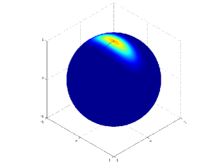
(a) $\kappa=25$, $\beta=10$

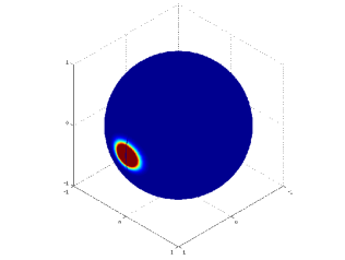
(b) $\kappa=100$, $\beta=10$

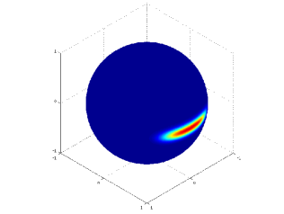
(c) $\kappa=100$, $\beta=49$

(d)

Figure 1: The Fisher-Bingham five-parameter (FB5) distribution $g(\widehat{\bm{x}};\kappa,\widehat{\bm{\mu}},\beta,\textbf{A})$, given in (9), is plotted on the sphere for parameters $\kappa$, $\beta$, as indicated and: (a) $\widehat{\bm{\mu}}=[0~{}0~{}1]^{T}$, $\widehat{\bm{\eta}}_{1}=[0~{}1~{}0]^{T}$, minor axis $\widehat{\bm{\eta}}_{2}=[1~{}0~{}0]^{T}$. (b) $\widehat{\bm{\mu}}=[1~{}0~{}0]^{T}$, $\widehat{\bm{\eta}}_{1}=[0~{}1~{}0]^{T}$, minor axis $\widehat{\bm{\eta}}_{2}=[0~{}0~{}1]^{T}$. (c) $\widehat{\bm{\mu}}=[0~{}1~{}0]^{T}$, $\widehat{\bm{\eta}}_{1}=[1~{}0~{}0]^{T}$, minor axis $\widehat{\bm{\eta}}_{2}=[0~{}0~{}1]^{T}$.

The FB5 distribution is more concentrated and more elliptic for larger values of $\kappa$ and $\beta$, respectively. As an example, the FB5 distribution $g(\widehat{\bm{x}};\kappa,\widehat{\bm{\mu}},\beta,\textbf{A})$ is plotted on the sphere in Fig. 1 for different values of parameters.

The FB5 distribution belongs to the family of spherical distributions in directional statistics and is the analogue of the Euclidean domain bivariate normal distribution with unconstrained covariance matrix [1, 5].

III-B 3D Spatial Fading Correlation (SFC)

In MIMO systems, the 3D multipath channel impulse response for a signal arriving at antenna array is characterized by the steering vector of the antenna array. For an antenna array consisting of $M$ antenna elements placed at $\bm{z}_{p}\in\mathbb{R}^{3},\,p=1,2,\dotsc,M$, the steering vector, denoted by $\bm{\alpha}(\widehat{\bm{x}})$, is given by

$$\bm{\alpha}(\widehat{\bm{x}})=\big{[}{\alpha}_{1}(\widehat{\bm{x}}),{\alpha}_{2}(\widehat{\bm{x}}),\dotsc{\alpha}_{L}(\widehat{\bm{x}})\big{]},\quad{\alpha}_{p}(\widehat{\bm{x}})\triangleq e^{ik\bm{z}_{p}\cdot\widehat{\bm{x}}},$$ (12)

where $\widehat{\bm{x}}\in\mathbb{R}^{3}$ denotes a unit vector pointing in the direction of wave propagation and $k=2\pi/\lambda$ with $\lambda$ denoting the wavelength of the arriving signal. For any $h(\widehat{\bm{x}})$ representing the pdf of the angles of arrival (AoA) of the multipath components or the unit-normalized power of a signal received from the direction $\widehat{\bm{x}}$, the 3D SFC function between the $p$-th and the $q$-th antenna elements, located at $\bm{z}_{p}$ and $\bm{z}_{q}$, respectively, with an assumption that signals arriving at the antenna elements are narrowband, is given by [21]

$$\rho(\bm{z}_{p},\bm{z}_{q}) \triangleq\int_{\mathbb{S}^{2}}h(\widehat{\bm{x}})\,\alpha_{p}(\widehat{\bm{x}})\,\overline{\alpha_{q}(\widehat{\bm{x}})}\,ds(\widehat{\bm{x}})$$

$$=\int_{\mathbb{S}^{2}}h(\widehat{\bm{x}})\,e^{ik(\bm{z}_{p}-\bm{z}_{q})\cdot\widehat{\bm{x}}}\,ds(\widehat{\bm{x}})\equiv\rho(\bm{z}_{p}-\bm{z}_{q}),$$ (13)

which indicates that the SFC only depends on $\bm{z}_{p}-\bm{z}_{q}$ and is, therefore, spatially wide-sense stationary.

III-C FB5 Distribution Based Spatial Correlation Model and Problem Under Consideration

The FB5 distribution offers the flexibility, due to its directional nature, to model the distribution of normalized power or AoA of the multipath components for most practical scenarios. Utilizing this capability of FB5 distribution, a 3D spatial correlation model for the mixture of FB5 distributions defining the AoA distribution has been developed in [9]. Here the mixture refers to the positive linear sum of a number of FB5 distributions, each with different parameters. We defer the formulation of FB5 based correlation model until Section V. Although the correlation model proposed in [9] is general in a sense that the SFC function can be computed for any arbitrary antenna geometry, the formulation of SFC function involves the computation of integrals that can only be carried out using numerical integration techniques as we highlighted earlier. If the spherical harmonic expansion of the FB5 distribution is given in closed-form, the SFC function can be computed analytically following the approach used in [21].

In this paper, we derive an exact expression to compute the spherical harmonic expansion of the FB5 distribution. Using the spherical harmonic expansion of FB5 distribution, we also formulate exact SFC function for the mixture of FB5 distributions, defining the distribution of AoA of the multipath components. We also analyse the computational considerations involved in the evaluation of spherical harmonic expansion of FB5 and distribution and SFC function.

(a)  $\kappa=25$, $\beta=10$,
$(\varphi,\vartheta,\omega)=(\pi/2,0,0)$.

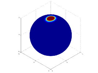
(b)  $\kappa=100$, $\beta=10$,
$(\varphi,\vartheta,\omega)=(\pi/2,\pi/2,0)$.

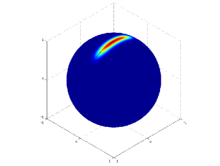
(c)  $\kappa=100$, $\beta=49$,
$(\varphi,\vartheta,\omega)=(\pi/2,\pi/2,\pi/2)$.

(d)

Figure 2: The standard Fisher-Bingham (FB) distribution $f(\widehat{\bm{x}};\kappa,\beta)$, given in (15), is plotted on the sphere for the concentration parameter $\kappa$ and ovalness parameter $\beta$, as indicated. Each subfigure is related to the respective subfigure of Fig. 1 through the the relation (16), with Euler angles indicated.

IV Spherical Harmonic Expansion of the FB5 Distribution

In this section, we derive an analytic expression for the computation of spherical harmonic coefficients of the FB5 distribution. For convenience, we determine the spherical harmonic coefficients of the FB5 distribution with mean (centre) $\widehat{\bm{\mu}}^{0}$ located on $z$-axis and major axis $\widehat{\bm{\eta}}_{1}^{0}$ and minor axis $\widehat{\bm{\eta}}_{2}^{0}$ aligned along $x$-axis and $y$-axis respectively, that is,

$$\widehat{\bm{\mu}}^{0}=[0~{}0~{}1]^{T}\quad\widehat{\bm{\eta}}_{1}^{0}=[1~{}0~{}0]^{T}\quad\widehat{\bm{\eta}}_{2}^{0}=[0~{}1~{}0]^{T}.$$ (14)

With the centre, major and minor axes as given in (14), the FB5 distribution, referred to as the standard Fisher-Bingham (FB) distribution, has the pdf given by

$$f(\widehat{\bm{x}};\kappa,\beta)\triangleq\frac{1}{C(\kappa,\beta)}e^{\kappa\cos\theta+\beta\sin^{2}\theta\cos 2\phi},$$ (15)

which is related to the FB5 distribution pdf $g(\widehat{\bm{x}};\kappa,\beta,\widehat{\bm{\mu}},\textbf{A})$ given in (9) through the rotation operator $\mathcal{D}(\varphi,\vartheta,\omega)$ as

$$g(\widehat{\bm{x}};\kappa,\beta,\widehat{\bm{\mu}},\textbf{A})=\left(\mathcal{D}(\varphi,\vartheta,\omega)f\right)(\widehat{\bm{x}};\kappa,\beta)=f(\bm{R}^{-1}\widehat{\bm{x}};\kappa,\beta),$$ (16)

where the rotation matrix is related to $\widehat{\bm{\mu}},~{}\widehat{\bm{\eta}}_{1},~{}\widehat{\bm{\eta}}_{2}$ (parameters of FB5 distribution) as

$$\bm{R}=[\widehat{\bm{\eta}}_{1},\widehat{\bm{\eta}}_{2},\widehat{\bm{\mu}}],$$ (17)

and the Euler angles $(\varphi,\vartheta,\omega)$ are related to the rotation matrix $\bm{R}$ through (8). As an example, we rotate each of the FB5 distribution $g(\widehat{\bm{x}};\kappa,\widehat{\bm{\mu}},\beta,\textbf{A})$ plotted in Fig. 1 to obtain the standard Fisher-Bingham distribution $f(\widehat{\bm{x}};\kappa,\beta)$, plotted in Fig. 2, where we have indicated the Euler angles that relate the FB5 distribution and the Fisher-Bingham distribution through (16).

IV-A Spherical Harmonic Expansion of Standard FB distribution

Here, we derive a closed-form expression to compute the spherical harmonic coefficients of the standard FB distribution, given in (15). Later in this section, noting the relation between standard FB distribution and FB5 distribution given in (16), and the effect of the rotation operation on the spherical harmonic coefficients, we determine the coefficients of FB5 distribution.

The spherical harmonic coefficient, denoted by $({f})_{\ell}^{m}$, of the standard Fisher-Bingham distribution given in (15) can be expressed as

$$({f})_{\ell}^{m}\triangleq\langle f(\,\cdot\,;\kappa,\beta),Y_{\ell}^{m}\rangle=\int_{\mathbb{S}^{2}}f(\widehat{\bm{x}};\kappa,\beta)\overline{Y_{\ell}^{m}(\widehat{\bm{x}})}ds(\widehat{\bm{x}}).$$ (18)

Since $f(\widehat{\bm{x}};\kappa,\beta)$ is a real function, we only need to compute the spherical harmonic coefficients for positive orders $0\leq m\leq\ell$ for each degree $\ell\geq 0$. The coefficients for the negative orders can be readily computed using the conjugate symmetry relation, noted in (6).

To derive a closed-form expression for computing the spherical harmonic coefficients, we rewrite (18) explicitly as

$$\begin{split}({f})_{\ell}^{m}&=\frac{N_{\ell}^{m}}{C(\kappa,\beta)}\int_{0}^{\pi}e^{\kappa\cos\theta}P_{\ell}^{m}(\cos\theta)\,\sin\theta d\theta\\ &\quad\quad\times\int_{0}^{2\pi}e^{-im\phi}e^{\beta\sin^{2}\theta\cos 2\phi}d\phi\\ &=\frac{N_{\ell}^{m}}{C(\kappa,\beta)}\int_{0}^{\pi}e^{\kappa\cos\theta}\,F_{m}(\theta)\,P_{\ell}^{m}(\cos\theta)\sin\theta d\theta,\end{split}$$

where

$$F_{m}(\theta)=\int_{0}^{2\pi}e^{\beta\sin^{2}\theta\cos 2\phi-im\phi}d\phi,$$

which we evaluate as 

$$\begin{split}F_{m}(\theta)&=\begin{cases}2\pi I_{m/2}(\beta\sin^{2}\theta)&m\in{0,\,2,\,4,\,\ldots}\\ 0&m\in{1,\,3,\,5,\,\ldots}.\end{cases}\end{split}$$

By expanding the modified Bessel function $I_{m/2}(\beta\sin^{2}\theta)$ as

$$I_{m/2}(\beta\sin^{2}\theta)=\sum_{t=0}^{\infty}\left(\frac{\beta}{2}\right)^{2t+m/2}\frac{(\sin\theta)^{4t+m}}{t!(t+m/2)!},$$ (19)

the exponential $e^{\kappa\cos\theta}$ as [8]

$$e^{\kappa\cos\theta}=\sqrt{\frac{\pi}{2\kappa}}\sum_{n=0}^{\infty}(2n+1)I_{n+1/2}(\kappa)P_{n}^{0}(\cos\theta),$$ (20)

and using the relation between associated Legendre polynomial and Wigner-$d$ function given in (3), along with the following expansion of Wigner-$d$ function in terms of complex exponentials

$$d^{\ell}_{m,n}(\theta)=i^{n-m}\sum_{u=-\ell}^{\ell}d_{u,m}^{\ell}({\pi}/{2})\,d_{u,n}^{\ell}({\pi}/{2})\,e^{iu\theta},$$ (21)

we obtain a closed-form expression for the spherical harmonic coefficient in (18) as

$$\begin{split}({f})_{\ell}^{m}&=\frac{\pi i^{-m}}{C(\kappa,\beta)}\sqrt{\frac{2\ell+1}{2\kappa}}\sum_{n=0}^{\infty}(2n+1)I_{n+1/2}(\kappa)~{}\times\\ &\sum_{u=-n}^{n}\left(d_{u,0}^{n}({\pi}/{2})\right)^{2}\sum_{t=0}^{\infty}\frac{(\beta/2)^{2t+m/2}}{\Gamma(t+1)\Gamma(t+m/2+1)}~{}\times\\ &\sum_{u^{\prime}=-\ell}^{\ell}d_{u^{\prime},0}^{\ell}({\pi}/{2})d_{u^{\prime},m}^{\ell}({\pi}/{2})\,G(4t+m+1,u+u^{\prime}),\end{split}$$ (22)

where $\Gamma(\cdot)$ denotes the Gamma function and we have used the following identity [27, Sec. 3.892]

$$G(p,q) \triangleq\int_{0}^{\pi}(\sin\theta)^{p}e^{iq\theta}d\theta,$$

$$=\frac{\pi e^{iq\pi/2}\Gamma(p+2)}{2^{p}(p+1)\Gamma(\frac{p+q+2}{2})\Gamma(\frac{p-q+2}{2})}\,.$$ (23)

IV-B Spherical Harmonic Expansion of FB5 distribution

We use the relation between standard FB distribution and FB5 distribution given in (16) to determine the spherical harmonic expansion of FB5 distribution. The Euler angles $(\varphi,\vartheta,\omega)$ in (16), which characterize the relation between the standard FB distribution and the FB5 distribution, can be obtained from the rotation matrix $\bm{R}$ formulated in (17) in terms of the parameters of FB5 distribution. By comparing (8) and (17), $\vartheta$ is given by

$$\vartheta=\cos^{-1}(R_{3,3}),$$ (24)

where $R_{a,b}$ denotes the entry at $a$-th row and $b$-th column of the matrix $\bm{R}$ given in (17). Similarly $\varphi\in[0,2\pi)$ and $\omega\in[0,2\pi)$ can be found by a four-quadrant search satisfying

$$\sin\varphi=\frac{R_{2,3}}{\sqrt{1-(R_{3,3})^{2}}},\quad\cos\varphi=\frac{R_{1,3}}{\sqrt{1-(R_{3,3})^{2}}},$$ (25)

$$\sin\omega=\frac{R_{3,2}}{\sqrt{1-(R_{3,3})^{2}}},\quad\cos\omega=\frac{-R_{3,1}}{\sqrt{1-(R_{3,3})^{2}}},$$ (26)

respectively.

Once the Euler angles $(\varphi,\vartheta,\omega)$ are extracted from the parameters $\widehat{\bm{\mu}},\widehat{\bm{\eta}}_{1},\widehat{\bm{\eta}}_{2}$ using (24)–(26), the spherical harmonic coefficients of the FB5 distribution $g(\widehat{\bm{x}};\widehat{\bm{\mu}},\kappa,\textbf{A})$ given in (9) can be computed following the effect of the rotation operation on the spherical harmonic coefficients as [26]

$$({g})_{\ell}^{m} \triangleq\langle g(\,\cdot\,;\widehat{\bm{\mu}},\kappa,\textbf{A}),Y_{\ell}^{m}\rangle=\langle\mathcal{D}(\varphi,\vartheta,\omega)f,Y_{\ell}^{m}\rangle$$

$$=\smashoperator[]{\sum_{m^{\prime}=-\ell}^{\ell}}\,D^{\ell}_{m,m^{\prime}}(\varphi,\vartheta,\omega)({f})_{\ell}^{m^{\prime}},$$ (27)

where $({f})_{\ell}^{m^{\prime}}$ is the spherical harmonic coefficient of degree $\ell$ and order $m^{\prime}$ of the standard Fisher-Bingham distribution $f(\widehat{\bm{x}})$. In (IV-B), $D^{\ell}_{m,m^{\prime}}(\varphi,\vartheta,\omega)$ denotes the Wigner-$D$ function of degree $\ell$ and orders $|m|,|m^{\prime}|\leq\ell$ and is given by [26]

$$D^{\ell}_{m,m^{\prime}}(\varphi,\vartheta,\omega)=\mathrm{e}^{-im\varphi}d^{\ell}_{m,m^{\prime}}(\vartheta)\mathrm{e}^{-im^{\prime}\omega}.$$ (28)

IV-C Computational Considerations

Here we discuss the computation of Wigner-$d$ functions, at a fixed argument of $\pi/2$, which are essentially required for the computation of spherical harmonic expansion of standard FB or FB5 distribution using the proposed formulation (22). Another computational consideration that is addressed here is the evaluation of infinite summations over $t$ and $n$ involved in the computation of (22).

IV-C1 Computation of Wigner-$d$ functions

For the computation of spherical harmonic coefficients of the standard FB distribution using (22), we are required to compute the Wigner-$d$ functions at a fixed argument of $\pi/2$, that is $d^{\ell}_{u,m}(\pi/2)$, for each $|u|,\,|m|\leq\ell$. Let $\mathbf{D}_{\ell}$ denote the matrix of size $(2\ell+1)\times(2\ell+1)$ with entries $d^{\ell}_{u,m}(\pi/2)$ for $|u|,|m|\leq\ell$. The matrix $\mathbf{D}_{\ell}$ can be computed for each $\ell=1,2,\dotsc,$ using the relation given in [28] that recursively computes $\mathbf{D}_{\ell}$ from $\mathbf{D}_{\ell-1}$.

IV-C2 Truncation over $n$

The infinite sum over $n$ arises from (20) where an exponential function of the concentration measure $\kappa$ and the co-latitude angle $\theta$ is expanded as an infinite sum of the modified Bessel functions and Legendre polynomials. It is well known that the Legendre polynomials are oscillating functions with a maximum value of one. The modified Bessel function $I_{n+1/2}(\kappa)$ that makes up the core of the expansion given in (20) decays quickly (and monotonically) to zero as $n\rightarrow\infty$ for a given $\kappa$. We use this feature of the modified Bessel function $I_{n+1/2}(\kappa)$ to truncate the summation over $n$. We plot $I_{n+1/2}(\kappa)$ for different values of $n$ and $0\leq\kappa\leq 100$ in Fig. 3, where it is evident that the Bessel function quickly decays to zero. We propose to truncate the summation over $n$ in (20), or equivalently in (22), at $n=N$ such that $I_{N+1/2}(\kappa)<10^{-16}$ (double machine precision). We approximate the linear relationship between such truncation level and the concentration parameter $\kappa$, given by

$$N=\frac{3}{2}\kappa+24,$$ (29)

which is also indicated in Fig. 3. This truncation level is found to give truncation error less than the machine precision level for the values of concentration parameter $\kappa$ in the range $0\leq\kappa\leq 100$ (used in practice [8, 9]). We note that the truncation error becomes smaller for large values of $\kappa$, indicating that the truncation at level less than $N$ given in (29) may also allow sufficiently accurate computation of spherical harmonic coefficients. Further analysis on establishing the relationship between the concentration parameter $\kappa$ and the truncation level is beyond the scope of current work.

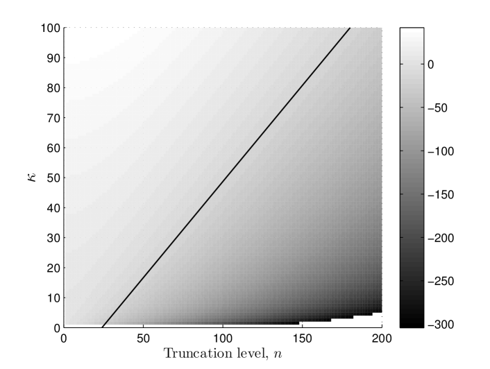
Figure 3: Surface plot of modified Bessel function $I_{n+1/2}(\kappa)$ for different values of $\kappa$ and $n$. The region $I_{n+1/2}(\kappa)<10^{-16}$ is approximated by the region below the straight line, $n=\frac{3}{2}\kappa+24$. Only those values $I_{n+1/2}(\kappa)>10^{-16}$ plotted above the straight line account for the sum in (20) to make it accurate to the machine precision level.

IV-C3 Truncation over $t$

The expansion of modified Bessel functions of the first kind for a given value of $\beta$ as given in (19) introduces the infinite sum over $t$. Again, the decaying (non-monotonic in this case) characteristics of the term inside the summation on right hand side of (19) with the increase in $t$ makes it possible to truncate the infinite sum given in (19) that mainly depends on the ovalness parameter $\beta$ with a minimal error. We plot the term inside the summation on the right hand side of (19) for $m=0$ and $\theta=\pi/2$, that is, $S(\beta,t)\triangleq\frac{\beta^{2t}}{t!t!\,2^{2t}}$ for different values of the ovalness parameter $\beta$ in Fig. 4. We again propose to truncate the summation over $t$ at the truncation level $T$ such that the terms after the truncation level $T$ are less than $10^{-16}$ and do not have impact on the summation. We approximate the linear relationship between the ovalness parameter $\beta$ and the truncation level $T$

$$T=\frac{36}{25}\beta+12.$$ (30)

Since we are computing coefficients for positive orders $0\leq m\leq\ell$ for each degree $\ell$, the truncation level given by (30), that is obtained for order $m=0$ and $\theta=\pi/2$, for the summation in (19), is also valid for all positive orders $0\leq m\leq\ell$ and all $\theta\in[0,\pi]$ because the term inside the summation is maximum for $m=0$ and $\theta=\pi/2$ for a given summation variable $t$.

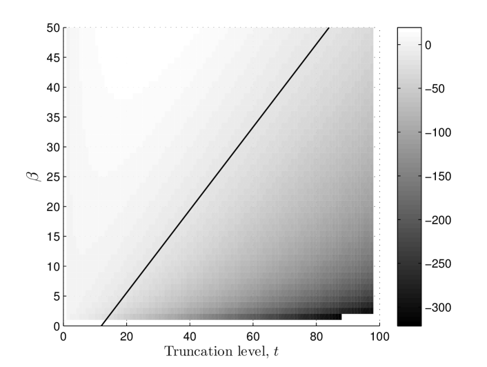
Figure 4: Surface plot of the term inside the summation on the right hand side of (19) for $m=0$ and $\theta=\pi/2$, that is, $S(\beta,t)\triangleq\frac{\beta^{2t}}{t!t!\,2^{2t}}$ for different values of the ovalness parameter $\beta$ and $t$. The region $R(\beta,t)<10^{-16}$ is approximated by the region below the straight line, $t=\frac{36}{25}\beta+12$.

We finally note that the truncation levels proposed here allow accurate computation of spherical harmonic coefficients to the level of double machine precision. Later in the paper, we validate the correctness of the derived expression for the computation of spherical harmonic coefficients of the standard FB distribution.

V 3D Spatial Fading Correlation for Mixture of Fisher-Bingham Distributions

In this section, we derive a closed form expression to compute the SFC function for the spatial correlation model based on a mixture of FB5 distributions defining the distribution of AoA of multipath components [8, 9]. Let $h(\widehat{\bm{x}})$ denotes the pdf of the distribution defined as a positive linear sum of $W$ FB5 distributions, each with different parameters, and is given by

$$h(\widehat{\bm{x}})=\sum_{w=1}^{W}K_{w}g(\widehat{\bm{x}};\kappa_{w},\widehat{\bm{\mu}}_{w},\beta_{w},\textbf{A}_{w}),$$ (31)

where $K_{w}$ denotes the weight of $w$-th FB5 distribution with parameters $\kappa_{w},\widehat{\bm{\mu}}_{w},\beta_{w}$ and $\textbf{A}_{w}$. We assume that each $K_{w}$ is normalized such that $\|h\|_{2}=1$. For the distribution with pdf defined in (31), the SFC function, given in (III-B) has been formulated in [9] and analysed for a uniform circular antenna array but the integrals involved in the SFC function were numerically computed.

We follow the approach introduced in [21] to derive a closed-form 3D SFC function using the proposed closed-form spherical harmonic expansion of the FB5 distribution. Using spherical harmonic expansion of plane waves [29]:

$$e^{ik\bm{z}_{p}\cdot\widehat{\bm{x}}}=4\pi\sum_{\ell=0}^{\infty}i^{\ell}j_{\ell}\big{(}k\lVert\bm{z}_{p}\rVert\big{)}\smashoperator[]{\sum_{m=-\ell}^{\ell}}\,Y_{\ell}^{m}\big{(}\bm{z}_{p}/\lVert\bm{z}_{p}\rVert\big{)}\overline{Y_{\ell}^{m}(\widehat{\bm{x}})},$$

and expanding the mixture distribution $h(\widehat{\bm{x}})$ in (31), following (4), and employing the orthonormality of spherical harmonics, we write the SFC function in (III-B) as [21]

$$\rho(\bm{z}_{p}-\bm{z}_{q}) =4\pi\sum_{\ell=0}^{\infty}i^{\ell}j_{\ell}\big{(}k\lVert\bm{z}_{p}-\bm{z}_{q}\rVert\big{)}~{}\times$$

$$\quad\smashoperator[]{\sum_{m=-\ell}^{\ell}}\,({h})_{\ell}^{m}Y_{\ell}^{m}\Big{(}\frac{\bm{z}_{p}-\bm{z}_{q}}{\lVert\bm{z}_{p}-\bm{z}_{q}\rVert}\Big{)},$$ (32)

where

$$({h})_{\ell}^{m} =\langle h,Y_{\ell}^{m}\rangle$$

$$=\sum_{w=1}^{W}\quad\smashoperator[]{\sum_{m^{\prime}=-\ell}^{\ell}}\,K_{w}D^{\ell}_{m,m^{\prime}}\,(\varphi_{w},\vartheta_{w},\omega_{w})({f})_{\ell}^{m^{\prime}},$$ (33)

which is obtained by combining (IV-B) and (31). Here, $({f})_{\ell}^{m^{\prime}}$ denotes the spherical harmonic coefficient of the standard FB distribution and the Euler angles $(\varphi_{w},\vartheta_{w},\omega_{w})$ relate the $w$-th FB5 distribution $g(\widehat{\bm{x}};\kappa_{w},\widehat{\bm{\mu}}_{w},\beta_{w},\textbf{A}_{w})$ of the mixture and the standard FB distribution $f(\widehat{\bm{x}})$ through (16). In the computation of the SFC using the proposed formulation, given in (V), we note that the summation for $\ell$ over first few terms yields sufficient accuracy as higher order Bessel functions decay rapidly to zero for points near each other in space, as indicated in [21, 30]. We conclude this section with a note that the SFC function can be analytically computed using the proposed formulation for an arbitrary antenna array geometry and the distribution of AoA modelled by a mixture of FB5 distributions, each with different parameters. In the next section, we evaluate the proposed SFC function for uniform circular array and a 3D regular dodecahedron array of antenna elements.

VI Experimental Analysis

We conduct numerical experiments to validate the correctness of the proposed analytic expressions, formulated in (22)–(IV-A) and (V)–(V), for the computation of the spherical harmonic coefficients of standard FB distribution and the SFC function for a mixture of FB5 distributions defining the distribution of AoA, respectively. For computing the spherical harmonic transform and discretization on the sphere, we employ the recently developed optimal-dimensionality sampling scheme on the sphere [31]. Our MATLAB based code to compute the spherical harmonic coefficients of the standard FB (or FB5) distribution and the SFC function using the results and/or formulations presented in this paper, is made publicly available.

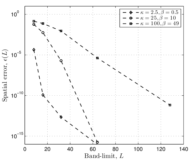
Figure 5: Spatial error $\epsilon(L)$, given in (34), between the standard FB distribution given in (15) and the reconstructed standard FB distribution from its coefficients up to the degree $L-1$. The convergence of the spatial error to zero (machine precision), as $L$ increases, corroborates the correctness of the derived spherical harmonic expansion of standard FB distribution.

VI-A Accuracy Analysis - Spherical Harmonic Expansion of standard FB distribution

In order to analyse the accuracy of the proposed analytical expression, for the computation of spherical harmonic coefficients of the standard FB distribution, given in (22), we define the spatial error as

$$\epsilon(L)=\frac{1}{L^{2}}\sum_{\widehat{\bm{x}}_{p}}\big{|}f(\widehat{\bm{x}}_{p})-\sum_{\ell=0}^{L-1}\sum_{m=-\ell}^{\ell}({f})_{\ell}^{m}Y_{\ell}^{m}(\widehat{\bm{x}}_{p})\big{|}^{2},$$ (34)

which quantifies the error between the standard FB distribution given in (15) and the reconstructed standard FB distribution from its coefficients, computed using the proposed analytic expression (22), up to the degree $L-1$. The summation in (34) is averaged over $L^{2}$ number of samples of the sampling scheme [31]. We plot the spatial error $\epsilon(L)$ against band-limit $L$ for different parameters of the standard FB distribution in Fig. 5, where it is evident that the spatial error converges to zero (machine precision) as $L$ increases. Consequently, the standard FB distribution reconstructed from its coefficients converges to the formulation of standard FB distribution in spatial domain and thus validates the correctness of proposed analytic expression.

VI-B Illustration - SFC Function

Here, we validate the proposed closed-form expression for the SFC function through numerical experiments. In our analysis, we consider both 2D and 3D antenna array geometries in the form of uniform circular array (UCA) and regular dodecahedron array (RDA), respectively. The antenna elements of $M$-element UCA are placed at the following spatial positions

$$\bm{z}_{p}=\big{[}R\cos\frac{2\pi p}{M},R\sin\frac{2\pi p}{M},0\big{]}^{T}\in\mathbb{R}^{3},$$ (35)

where $R$ denotes the circular radius of the array. For the RDA, 20 antenna array elements are positioned at the vertices of a regular dodecahedron inscribed in a sphere of radius $R$, as shown in Fig. 6 for $R=1$. We assume that the AoA follows a standard Fisher-Bingham distribution.

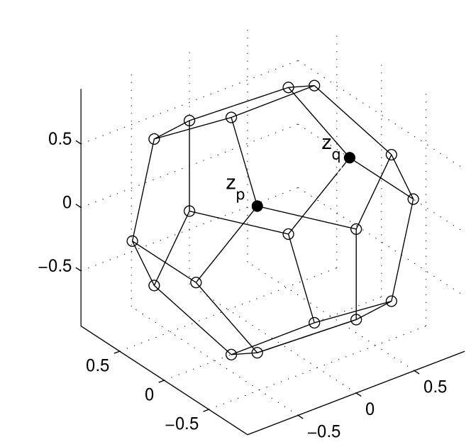
Figure 6: Regular dodecahedron array (RDA) – 20 antenna elements positioned at the vertices of a regular dodecahedron inscribed in a sphere of radius $R=1$.

Using the proposed closed-form expression in (V), we determine the SFC between the second and third UCA antenna elements and plot the magnitude of the SFC function $\rho(\bm{z}_{2}-\bm{z}_{3})$ in Fig. 7 against the normalized radius $R/\lambda$. In the same figure, we also plot the numerically evaluated SFC function, formulated in (III-B) and originally proposed in [9], which matches with the proposed closed-form expression for the SFC function. We emphasise that numerical evaluation of the integrals employs computationally intensive techniques to obtain sufficiently accurate results and is therefore time consuming. Similarly, we compute the SFC between two antenna elements positioned at $\bm{z}_{p}$ and $\bm{z}_{q}$ on RDA, which are indicated in Fig. 6, and plot the magnitude $\rho(\bm{z}_{p}-\bm{z}_{q})$ Fig. 6, which again matches with the numerically evaluated SFC function given in (III-B) and thus corroborates the correctness of proposed SFC function.

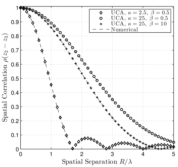
Figure 7: Magnitude of the SFC function $\rho(\bm{z}_{2}-\bm{z}_{3})$ for $16$-element UCA of radius $R$.

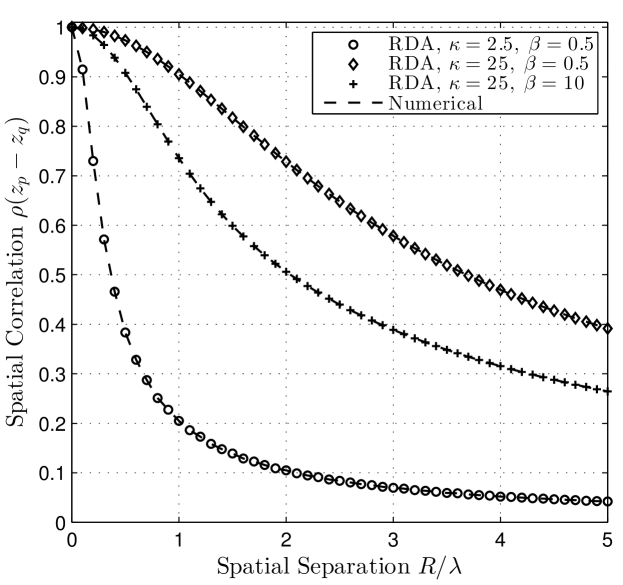
Figure 8: Magnitude of the SFC function $\rho(\bm{z}_{p}-\bm{z}_{q})$ between antenna elements, placed at vertices shaded in black in Fig. 6, of $20$-element RDA of radius $R$.

VII Conclusions

In this paper, the spherical harmonic expansion of the Fisher-Bingham distribution and a closed-form expression that allows the analytic computation of the spherical harmonic coefficients have been presented. Using the expansion of plane waves in spherical harmonics and the proposed closed-form expression for the spherical harmonic coefficients of the FB5 distribution, we derived an analytic formula for the 3D SFC function between two arbitrary points in 3D-space when the AoA of an incident signal has the Fisher-Bingham distribution. Furthermore, we have validated the correctness of proposed closed-form expressions for the spherical harmonic coefficients of the Fisher-Bingham distribution and the 3D SFC using numerical experiments. We have focussed on the use of Fisher-Bingham distribution for the computation of SFC function. However, we believe that the proposed spherical harmonic expansion of the Fisher-Bingham distribution has a great potential of applicability in various applications for directional statistics and data analysis on the sphere.

References

- [1] J. T. Kent, “The Fisher-Bingham distribution on the sphere,” J. R. Statist. Soc., vol. 44, no. 1, pp. 71–80, Jun. 1982.
- [2] P. Leong and S. Carlile, “Methods for spherical data analysis and visualization,” J. Neuro. Metho., vol. 80, no. 2, pp. 191–200, 1998.
- [3] E. H. Langendijk, D. J. Kistler, and F. L. Wightman, “Sound localization in the presence of one or two distracters,” J. Acoust. Soc. Am., vol. 109, no. 5, pp. 2123–2134, 2001.
- [4] D. Peel, W. J. Whiten, and G. J. McLachlan, “Fitting mixtures of kent distributions to aid in joint set identification,” J. American Statistical Asociation, vol. 96, no. 453, pp. 56–63, 2001.
- [5] J. T. Kent and T. Hamelryck, “Using the Fisher-Bingham distribution in stochastic models for protein structure,” In Barber S, Baxter P, Mardia K, Walls R, eds. Quantitative Biology, Shape ANalysis and Wavelets, Leeds University Press, Leeds, UK, vol. 24, pp. 57–60, 2005.
- [6] C. T. Christou, “Beamforming spatially spread signals with the kent distribution,” in Proc. IEEE Int. Conf. on Information Fusion, 2008, pp. 1–7.
- [7] D. Lunga and O. Ersoy, “Kent mixture model for classification of remote sensing data on spherical manifolds,” in Applied Imagery Pattern Recognition Workshop (AIPR), 2011 IEEE. IEEE, 2011, pp. 1–7.
- [8] K. Mammasis and R. W. Stewart, “The FB5 distribution and its application in wireless communications,” in Proc. of Int. ITG Workshop on Smart Antennas, pp. 375–381, Feb. 2008.
- [9] K. Mammasis and R. W. Stewart, “The Fisher-Bingham spatial correlation model for multielement antenna systems,” IEEE Trans. Veh. Technol., vol. 58, no. 5, pp. 2130–2136, Jun. 2009.
- [10] J. Salz and J. H. Winters, “Effect of fading correlation on adaptive arrays in digital mobile radio,” IEEE Trans. Veh. Technol., vol. 43, no. 4, pp. 1049–1057, Nov. 1994.
- [11] L. Fang, G. Bi, and A. C. Kot, “New method of performance analysis for diversity reception with correlated rayleigh-fading signals,” IEEE Trans. Veh. Technol., vol. 49, no. 5, pp. 1807–1812, 2000.
- [12] D. S. Shiu, G. J. Foschini, M. J. Gans, and J. M. Kahn, “Fading correlation and its effect on the capacity of multielement antenna systems,” IEEE Trans. Commun., vol. 48, no. 3, pp. 502–513, Mar. 2000.
- [13] A. Abdi and M. Kaveh, “A space-time correlation model for multielement antenna systems in mobile fading channels,” IEEE J. Sel. Areas Commun., vol. 20, no. 3, pp. 550–560, 2002.
- [14] J.-A. Tsai, R. M. Buehrer, and B. D. Woerner, “BER performance of a uniform circular array versus a uniform linear array in a mobile radio environment,” IEEE Trans. Wireless Commun., vol. 3, no. 3, pp. 695–700, 2004.
- [15] R. A. Kennedy, P. Sadeghi, T. D. Abhayapala, and H. M. Jones, “Intrinsic limits of dimensionality and richness in random multipath fields,” IEEE Trans. Signal Process., vol. 55, no. 6, pp. 2542–2556, Jun. 2007.
- [16] M. Kalkan and R. H. Clarke, “Prediction of the space-frequency correlation function for base station diversity reception,” IEEE Trans. Veh. Technol., vol. 46, no. 1, pp. 176–184, Feb. 1997.
- [17] K. I. Pedersen, P. E. Mogensen, and B. H. Fleury, “Power azimuth spectrum in outdoor environments,” Electron. Lett., vol. 33, no. 18, pp. 1583–1584, 1997.
- [18] R. G. Vaughan, “Pattern translation and rotation in uncorrelated source distributions for multiple beam antenna design,” IEEE Trans. Antennas Propag., vol. 46, no. 7, pp. 982–990, Jul. 1998.
- [19] A. Abdi and M. Kaveh, “A versatile spatio-temporal correlation function for mobile fading channels with non-isotropic scattering,” in Proc. Tenth IEEE Workshop on Statistical Signal and Array Processing, Pocono Manor, PA, Aug. 2000, pp. 58–62.
- [20] J.-A. Tsai, R. Buehrer, and B. Woerner, “Spatial fading correlation function of circular antenna arrays with laplacian energy distribution,” IEEE Commun. Lett., vol. 6, no. 5, pp. 178–180, May 2002.
- [21] P. D. Teal, T. D. Abhayapala, and R. A. Kennedy, “Spatial correlation for general distributions of scatterers,” IEEE Signal Process. Lett., vol. 9, no. 10, pp. 305–308, Oct. 2002.
- [22] S. K. Yong and J. Thompson, “Three-dimensional spatial fading correlation models for compact mimo receivers,” IEEE Trans. Wireless Commun., vol. 4, no. 6, pp. 2856–2869, Nov. 2005.
- [23] K. Mammasis and R. W. Stewart, “Spherical statistics and spatial correlation for multielement antenna systems,” EURASIP Journal on Wireless Communication and Networking, vol. 2010, Dec. 2010.
- [24] J.-H. Lee and C.-C. Cheng, “Spatial correlation of multiple antenna arrays in wireless communication systems,” Progress in Electromagnetics Research, vol. 132, pp. 347–368, 2012.
- [25] R. A. Kennedy, Z. Khalid, and Y. F. Alem, “Spatial correlation from multipath with 3D power distributions having rotational symmetry,” in Proc. Int. Conf. Signal Processing and Communication Systems, ICSPCS’2013, Gold Coast, Australia, Dec. 2013, p. 7.
- [26] R. A. Kennedy and P. Sadeghi, Hilbert Space Methods in Signal Processing. Cambridge, UK: Cambridge University Press, Mar. 2013.
- [27] A. Jeffrey and D. Zwillinger, Table of integrals, series, and products. Academic Press, 2007.
- [28] S. Trapani and J. Navaza, “AMoRe: Classical and modern,” Acta Crystallogr. Sect. D, vol. 64, no. 1, pp. 11–16, Jan. 2008.
- [29] D. Colton and R. Kress, Inverse Acoustic and Electromagnetic Scattering Theory, 3rd ed. New York, NY: Springer, 2013.
- [30] H. M. Jones, R. A. Kennedy, and T. D. Abhayapala, “On dimensionality of multipath fields: Spatial extent and richness,” in Proc. IEEE Int. Conf. Acoustics, Speech, and Signal Processing, ICASSP’2002, vol. 3, Orlando, FL, May 2002, pp. 2837–2840.
- [31] Z. Khalid, R. A. Kennedy, and J. D. McEwen, “An optimal-dimensionality sampling scheme on the sphere with fast spherical harmonic transforms,” IEEE Trans. Signal Process., vol. 62, no. 17, pp. 4597–4610, Sep. 2014.