Isolation in the construction of natural experiments

Abstract

A natural experiment is a type of observational study in which treatment assignment, though not randomized by the investigator, is plausibly close to random. A process that assigns treatments in a highly nonrandom, inequitable manner may, in rare and brief moments, assign aspects of treatments at random or nearly so. Isolating those moments and aspects may extract a natural experiment from a setting in which treatment assignment is otherwise quite biased, far from random. Isolation is a tool that focuses on those rare, brief instances, extracting a small natural experiment from otherwise useless data. We discuss the theory behind isolation and illustrate its use in a reanalysis of a well-known study of the effects of fertility on workforce participation. Whether a woman becomes pregnant at a certain moment in her life and whether she brings that pregnancy to term may reflect her aspirations for family, education and career, the degree of control she exerts over her fertility, and the quality of her relationship with the father; moreover, these aspirations and relationships are unlikely to be recorded with precision in surveys and censuses, and they may confound studies of workforce participation. However, given that a women is pregnant and will bring the pregnancy to term, whether she will have twins or a single child is, to a large extent, simply luck. Given that a woman is pregnant at a certain moment, the differential comparison of two types of pregnancies on workforce participation, twins or a single child, may be close to randomized, not biased by unmeasured aspirations. In this comparison, we find in our case study that mothers of twins had more children but only slightly reduced workforce participation, approximately 5% less time at work for an additional child.

FLA

, and T2Supported by NSF Grant SES-1260782.

1 Constructing natural experiments.

1.1 Natural experiments.

Natural experiments are a type of observational study, that is, a study of the effects caused by treatments when random assignment is infeasible or unethical. What distinguishes a natural experiment from other observational studies is the emphasis placed upon finding unusual circumstances in which treatment assignment, though not randomized, seems to resemble randomized assignment in that it is haphazard, not the result of deliberation or considered judgement, not confounded by the typical attributes that determine treatment assignment in a particular empirical field. The literature on natural experiments spans the health and social sciences; see, for instance, Arpino and Aassve (2013), Imai et al. (2011), Meyer (1995), Rutter (2007), Sekhon and Titiunik (2012), Susser (1981) and Vandenbroucke (2004).

Traditionally, natural experiments were found, not built. In one sense, this seemed inevitable: one needs to find haphazard treatment assignment in a world that typically assigns treatments in a biased fashion, often assigning treatments with a view to achieving an objective. There is, however, substantial scope for constructing natural experiments. When treatment assignment is biased, there may be aspects of treatment assignment, present only briefly, that are haphazard, close to random. The key to constructing natural experiments is to isolate these transient, haphazard aspects from typical treatment assignments that are biased. If brief haphazard aspects of treatment assignment can be isolated from the rest, in the isolated portion it is these haphazard elements that are decisive. This is analogous to a laboratory in which a treatment is studied in isolation from disruptions that would obscure the treatment’s effects. Laboratories are built, not found.

1.2 A natural experiment studying effects of fertility on workforce participation.

Does having a child reduce a mother’s participation in the workforce? If it does, what is the magnitude of the reduction? The question is relevant to individuals planning families and careers and to legislators and managers who determine policies related to fertility, such as family leaves. A major barrier to answering this question is that, for many if not most women, decisions about fertility, education and career are highly interconnected, and each decision has consequences for the others. Here we follow Angrist and Evans (1998) and seek to determine if there is some source of variation in fertility that does not reflect career plans and is just luck. Although a woman has the ability to influence the timing of her pregnancies, given that she is pregnant at a particular age, she has much less influence about whether she will have a boy or a girl, whether she will have a single child or twins—to a large extent, that is just luck. More precisely, that a woman is pregnant at a certain moment in her life may be indicative of her unrecorded plans and aspirations for education, family and career, but conditionally given that she is pregnant at that moment, the birth outcome, a boy or a girl or twins, is unlikely to indicate much about her plans and aspirations.

We focus here on the haphazard contrast most likely to shift the total number of children, namely, a comparison of similar women, one with a twin at her $k$th birth, the other with children of mixed sex at her $k$th birth since, as Angrist and Evans (1998) noted, many women or families in the US prefer to have children of both sexes, rather than just boys or just girls, that is, a third child is seen in data to be more common if the first two children have the same sex. While we could compare women having twins with women having a single child whose sex is the same as her first child, we focus on comparing women having twins with women having a single child whose sex is different from her first since the first woman may end up with one more child than she intended, whereas the other woman will, at least, not have additional children simply to have one of each sex.

What question does such a natural experiment answer? Conditionally given that a woman with a certain prior history of fertility is currently pregnant, having a girl or a boy or twins does not pick out a particular type of woman. So the study is accepting whatever process led a particular woman to be pregnant at a certain moment in her life, and it is asking: What would happen if she unexpectedly had two children at that pregnancy rather than one? How would that event alter her subsequent workforce participation? We use the idea from Angrist and Evans (1998) to illustrate and discuss tools to extract natural experiments from larger biased data sets, in particular, risk set matching [Li, Propert and Rosenbaum (2001)], differential effects [Rosenbaum (2006, 2013a)] and strengthening an instrumental variable [Baiocchi et al. (2010), Zubizarreta et al. (2013)].

1.3 Informal review of two key concepts: Differential effects; risk-setmatching.

Because differential effects and risk set matching may be unfamiliar, we now review the motivation for these techniques. Consider, first, differential effects and generic biases acting at a single point in time [Rosenbaum (2006, 2013a)]. Treatment assignment may be biased by certain unmeasured covariates that promote several treatments in a similar way. When this is true, receiving a treatment $s$ may be very biased by these covariates, while receiving one treatment $s$ in lieu of another $s^{\prime}$ may be unbiased or less biased or biased in a different way. Here, attention shifts from whether or not a person received treatment $s$ (i.e., the main effect of $s$) to whether a person received treatment $s$ rather than treatment $s^{\prime}$ conditionally given that the person received either treatment $s$ or treatment $s^{\prime}$ (i.e., the differential effect of $s$ in lieu of $s^{\prime}$). Consider an example discussed in detail by Anthony et al. (2000). There is a theory that nonsteroidal anti-inflammatory drugs (NSAIDs), such as ibuprofen (e.g., brand Advil), may reduce the risk of Alzheimer disease. There is an obvious bias in comparing people who regularly take ibuprofen and people who do not. In all likelihood, a person who regularly takes ibuprofen is experiencing chronic pain, perhaps arthritis or back pain, is aware of that pain, and is capable of acting deliberately on the basis of that awareness. It has been suggested that people in the early undiagnosed stages of Alzheimer disease are less aware of pain and less able to act on what awareness they have, so that fact alone might produce a spurious association between use of ibuprofen and lower risk of later diagnosed Alzheimer disease. There are, however, pain relievers that are not NSAIDs, for example, acetaminophen (e.g., brand Tylenol). While limited awareness of pain or limited ability to act on awareness might reduce use of pain relievers of all kinds, it seems far less plausible that it shifts people away from ibuprofen and toward acetaminophen. That is, the differential effect of acetaminophen-versus-ibuprofen—of one treatment in lieu of the other—may not be biased by unmeasured covariates that would bias straightforward estimates of the main effect of either drug. Differential effects are not main effects, but when differential effects are interesting, they may be immune to certain biases that distort main effects. See also Gibbons et al. (2010) for differential effects in the study of medications.

Consider, second, risk-set matching, a device for respecting the temporal structure of treatment assignment in observational studies [Li, Propert and Rosenbaum (2001)]. For each subject in a randomized experiment, there is a specific moment at which this subject is assigned to treatment or to control. In some observational studies, there is no corresponding moment. Some people receive treatment at a specific time, others receive it later or never receive it, but anyone who does not receive treatment today might receive it tomorrow. Risk-set matching pairs two individuals at a specific time, two individuals who looked similar in observed covariates prior to that specific time, a time at which one individual was just treated and the other was not-yet-treated. The not-yet-treated individual may be treated tomorrow, next year or never. We compare two individuals who looked similar prior to the moment that one of them was treated, avoiding matching or adjustment for events subsequent to that moment [cf. Rosenbaum (1984)]. That is, in the language of Cox’s proportional hazards model, risk-set matching pairs two individuals who were both at risk of receiving the treatment a moment before one of them actually received it, two individuals who looked similar in time-dependent covariates prior to that moment. Taken alone, without differential comparisons, risk-set matching is a method for controlling measured time-dependent covariates respecting the temporal structure of treatment assignment; see van der Laan and Robins (2003) for other methods for this task.

1.4 Outline of the paper.

Section 2 discusses new relevant theory, specifically theory linking risk-set matching for time-dependent measured covariates with differential comparisons unaffected by certain unmeasured time dependent covariates. Fertility is commonly modeled in terms of “event history” or point process models determining the timing of events together with “marks” or random variables describing these randomly timed events. The mark may record the occurrence of twins. Temporal order is key and must be respected. Sections 3 and 4 complete the case study of twin births with the construction of the matched sample using combinatorial optimization for risk-set matching discussed in Section 3 and a detailed analysis presented in Section 4. Section 5 includes a discussion of related work.

2 Risk-set matching to control generic unmeasured biases.

2.1 Notation for treatments over time.

The population before matching contains statistically independent individuals. At time $t$, individual $\ell$ has a history of events prior to $t$, the observed history being recorded in $\mathbf{x}_{\ell t}$ and the unobserved history being recorded in $u_{\ell t}$. To avoid a formal notation that we would rarely use, we write histories as variables, $\mathbf{x}_{\ell t}$ or $u_{\ell t}$, but we intend to convey a little more than this. Both the quantity and types of information in $\mathbf{x}_{\ell t}$ or in $u_{\ell t}$ or in $(\mathbf{x}_{\ell t},u_{\ell t})$ increase as time passes, that is, as $t$ increases [or, formally, the sigma algebra generated by $(\mathbf{x}_{\ell t},u_{\ell t})$ is contained within the sigma algebra generated by $(\mathbf{x}_{\ell t^{\prime}},u_{\ell t^{\prime}})$ for $t<t^{\prime}$].

In our case study, $\mathbf{x}_{\ell t}$ records such things as the ages at which mother $\ell$ gave birth to the children she had prior to time $t$, her years of education attained at the times of those births before time $t$, and unchanging characteristics such as her place of birth, race or ethnicity. In parallel, $u_{\ell t}$ might be an unmeasured quantity reflecting the entire history of a woman’s inclination to work full time in the year subsequent to time $t$. Obviously, a birth at time $t$ might, often would, alter $\mathbf{x}_{\ell t^{\prime}}$ or $u_{\ell t^{\prime}}$ for $t^{\prime}>t$.

There is also a treatment process $Z_{\ell t}$ that is in one of $K+1$ states, $s_{0}$, $s_{1},\ldots,s_{K}$. That is, at any time $t$, individual $\ell$ is in exactly one of these states, $Z_{\ell t}=s_{k}$ for some $k\in\{0,1,\ldots,K\}$. Also, write $\overline{Z}_{\ell t}$ for the history of the $Z_{\ell t}$ process strictly prior to time $t$, so $\overline{Z}_{\ell t}$ records $Z_{\ell t^{\prime}}$ for $t^{\prime}<t$ but it does not record $Z_{\ell t}$. In our case study, state $s_{0}$ is the interval state of not currently giving birth to a child, state $s_{1}$ is the point state of giving birth to a single female child, state $s_{2}$ is the point state of giving birth to a single male child, state $s_{3}$ is the point state of giving birth to a pair of female twins and so on. Most women are in state $Z_{\ell t}=s_{0}$ at most times $t$. The history $\overline{Z}_{\ell t}$ records mother $\ell$’s births up to time $t$, their timing, the sex of the child, twins, etc.

Consider a specific individual $\ell$ at a specific time $t$. At this moment, the individual has a treatment history $\overline{Z}_{\ell t}$ prior to $t$ and is about to receive a current treatment $Z_{\ell t}$. Given the past, $\overline{Z}_{\ell t}$, we are interested in the effect of the current treatment $Z_{\ell t}$ on some future (i.e., after $t$) outcome $R_{\ell}$. Write $\mathcal{F}_{\ell t}=(\overline{Z}_{\ell t},\mathbf{x}_{\ell t},u_{\ell t})$ for the past at time $t$. In parallel with Neyman (1923) and Rubin (1974), this individual $\ell$ at this time $t$ has $K+1$ possible values for $R_{\ell}$ depending upon the treatment $Z_{\ell t}$ assigned at time $t$, that is, $R_{\ell}=r_{k\ell}$ if $Z_{\ell t}=s_{k}$, where only one $R_{\ell}$ is observed from an individual, and the effect of giving treatment $k$ rather than $k^{\prime}$ at time $t$, namely, $r_{k\ell}-r_{k^{\prime}\ell}$ is not observed for any person at any time. This structure is for individual $\ell$ at a specific time $t$ with treatment history $\overline{Z}_{\ell t}$; typically, everything about this structure would change if the history $\overline{Z}_{\ell t}$ to time $t$ had been different. The question is what effect treatment at time $t$ has on an individual with a specific treatment and covariate history prior to $t$. It is entirely possible—indeed, in typical applications, it is likely—that the treatments $Z_{\ell t^{\prime}}$ at times $t^{\prime}<t$ alter the value of observed or unobserved subsequent history $(\mathbf{x}_{\ell t},u_{\ell t})$, but the history at $t$, namely, $(\mathbf{x}_{\ell t},u_{\ell t})$, records the situation just prior to $t$ and hence is unaffected by the treatment assignment $Z_{\ell t}$ at $t$. Quite often, the outcome $R_{\ell}$ is a future value of a quantity that is analogous to a past quantity recorded in the history $(\mathbf{x}_{\ell t},u_{\ell t})$. In our case study, $R_{\ell}$ might measure an aspect of future workforce participation beyond time $t$ where $(\mathbf{x}_{\ell t},u_{\ell t})$ records workforce participation prior to time $t$, or $R_{\ell}$ might measure educational attainment at some time after $t$ where $(\mathbf{x}_{\ell t},u_{\ell t})$ records educational attainment prior to time $t$.

In our case study, aspects of the record of a woman’s fertility, $Z_{\ell t}$, are likely to be strongly predicted by aspects of her observed and unobserved histories $(\mathbf{x}_{\ell t},u_{\ell t})$. A woman $\ell$ aged $t^{\prime}=18$ years whose private aspiration $u_{\ell t}$ is to earn a Ph.D. in molecular biology and an MBA and to start her own biotechnology company is likely to take active steps to ensure $Z_{\ell t}=s_{0}$ for $t\in(18,22]$ or longer, that is, she is likely to postpone having children for at least several years. In contrast, another woman $\ell^{\prime}$ whose private aspiration $u_{\ell^{\prime}t}$ at age $t^{\prime}=18$ is to stay at home as the mother of many children may take active steps to ensure $Z_{\ell t}\neq s_{0}$ for several $t\in(18,22]$, that is, she may actively pursue her goal of a large family. A comparison of the workforce participation of woman $\ell$ and woman $\ell^{\prime}$ will be severely biased as an estimate of the effects of having a child before age 22 on workforce participation, because $\ell$ tried to shape her fertility to fit her work plans and $\ell^{\prime}$ tried to shape her fertility to fit her family plans—even if, by some accident, they had the same pattern of fertility over $t\in(18,22]$, we would not be surprised to learn that $\ell$ subsequently worked more for pay than did $\ell^{\prime}$. What is an investigator to do when unmeasured aspirations, intentions and goals are strongly associated with treatment assignment?

2.2 What is risk-set matching?

Risk-set matching compares people, say, $\ell$ and $\ell^{\prime}$, who received different treatments at time $t$, $Z_{\ell t}\neq Z_{\ell^{\prime}t}$, but who looked similar in their observed histories prior to $t$, $\mathbf{x}_{\ell t}=\mathbf{x}_{\ell^{\prime}t}$ and $\overline{Z}_{\ell t}=\overline{Z}_{\ell^{\prime}t}$; see Li, Propert and Rosenbaum (2001), Lu (2005) and Rosenbaum [(2010), Section 12]. Importantly, $\ell$ and $\ell^{\prime}$ are similar prior to $t$ in terms of observable quantities that may be controlled by matching, but they may not be similar in terms of unmeasured histories, $u_{\ell t}\neq u_{\ell^{\prime}t}$, and of course they may differ in the future, after time $t$, not least because they received different treatments at time $t$. Risk-set matching does not solve the problem of unmeasured histories. Risk-set matching does respect the temporal structure of the data, avoiding adjustment for variables affected by the treatment [Rosenbaum (1984)]. Risk-set matching also “simplifies the conditions of observation,” to use Mervyn Susser’s [(1973), Section 7] well-chosen phrase, ensuring that comparisons are of people with histories that look comparable, even though those histories may be of different lengths, and hence may contain qualitatively different information. Although individuals have histories of different lengths containing qualitatively different information, matched individuals have histories of the same length. For instance, a woman giving birth to her 3rd child has in her history ages of birth of her first three children, where a mother giving birth to her second child does not have in her history her age at the birth of her third child, if indeed she had a third child.

In implementing risk-set matching in Section 3, we match women of the same age, with the same history of fertility—the same numbers of prior children born at the same ages in the same patterns. We also control for temporally fixed quantities associated with fertility, such as ethnicity. A delicate issue that risk-set matching would straightforwardly address with adequate data is “education.” On the one hand, education is strongly related to wage income and is related to employment, so it may strongly predict certain workforce outcomes $R_{\ell}$. On the other hand, education may itself be affected by fertility: a mother who has her first child at age 16 may as a consequence have difficulty completing high school. In principle, the issue is straightforward with risk-set matching: in studying the effects of fertility $Z_{\ell t}$ at time $t$, one compares two people who had the same education prior to $t$, without equating their educations subsequent to time $t$. Again, this avoids adjustment for variables affected by the treatment [Rosenbaum (1984)]. If the adjustment for education at time $t$ controlled for subsequent education at time $t^{\prime}>t$, it might—probably would—remove a substantial part of the actual effect on workforce participation of having a child at age 16. Not finishing high school is a good way to have trouble in the labor market, and having a child at age 16 is a good way to have trouble finishing high school; everyone remembers this until they start running regressions, but then, too often, part of an actual effect is removed by adjusting for a posttreatment variable that was also affected by the treatment.

Risk-set matching was discussed by Li, Propert and Rosenbaum (2001) and Lu (2005). It has been applied in criminology [Nieuwbeerta, Nagin and Blokland (2009), Apel et al. (2010), Murray, Loeber and Pardini (2012)], sociology [Wildeman, Schnittker and Turney (2012)] and medicine [Kennedy et al. (2010)]. See Marcus et al. (2008), Rosenbaum [(2010), Section 12], Stuart (2010) and Lu et al. (2011) for related discussion.

2.3 Removing generic unmeasured biases by differential comparisons in risk sets.

The model for biased treatment assignment in risk-set matching is intended to express the thought that matching for the observed past, $(\overline{Z}_{\ell t},\mathbf{x}_{\ell t})$, has controlled for the observed past but typically did not control for the unobserved past $u_{\ell t}$. The model is a slight generalization to multiple states of the model for two states in Li, Propert and Rosenbaum [(2001), Section 4], and that model is itself closely patterned after Cox’s (1972) proportional hazards model for outcomes rather than treatments. People are in state $s_{0}$ almost all the time, and are in states $s_{1},\ldots,s_{K}$ only at points in time. Let $\lambda_{k}(\mathcal{F}_{\ell t})=\lambda_{k}(\overline{Z}_{\ell t},\mathbf{x}_{\ell t},u_{\ell t})$ be the hazard, assumed to exist, of entering state $k\geq 1$ at time $t$ given past $\mathcal{F}_{\ell t}$. The hazard is assumed to be of the form $\lambda_{k}(\overline{Z}_{\ell t},\mathbf{x}_{\ell t},u_{\ell t})=\exp\{\kappa_{k}(\overline{Z}_{\ell t},\mathbf{x}_{\ell t})+\phi_{k}u_{\ell t}\}$ where $\kappa_{k}(\cdot,\mathbf{\cdot})$ is unknown. Because $\mathbf{x}_{\ell t}$ may include as one of its coordinates the time $t$, this model permits the hazards to vary with time $t$. For state $s_{0}$, it is notationally convenient to define $\lambda_{0}(\cdot,\mathbf{\cdot},\cdot)=1$ and $\phi_{0}=0$.

In Section 2.1, $u_{\ell t}$ was described as a possibly multivariate history of a possibly continuous process in time, whereas in the hazard model,$\exp\{\kappa_{k}(\overline{Z}_{\ell t},\mathbf{x}_{\ell t})+\phi_{k}u_{\ell t}\}$, the unobserved element has become a scalar. This seems at first to be an enormous and disappointing loss of generality, but upon reflection one sees that the loss is not great. Suppose $u_{\ell t}$ did record a multivariate history over time, and consider the hazard model $\exp\{\kappa_{k}(\overline{Z}_{\ell t},\break\mathbf{x}_{\ell t})+\phi_{k}f(u_{\ell t})\}$ where $f(\cdot)$ is some unknown real-valued functional of that multivariate, temporal history. Although this appears at first to be a more general model, writing $\widetilde{u}_{i\ell}=f(u_{\ell t})$, the model becomes $\exp\{\kappa_{k}(\overline{Z}_{\ell t},\mathbf{x}_{\ell t})+\phi_{k}\widetilde{u}_{i\ell}\}$, a scalar model essentially as before. In words, in $\exp\{\kappa_{k}(\overline{Z}_{\ell t},\mathbf{x}_{\ell t})+\phi_{k}f(u_{\ell t})\}$, not knowing $u_{\ell t}$ and not knowing $f(\cdot)$ is no better and no worse than not knowing the scalar $\widetilde{u}_{i\ell}=f(u_{\ell t})$. It is the impact of unmeasured history on the hazard—a scalar—that matters, not the particulars of that history. See Li, Propert and Rosenbaum (2001) and Lu (2005) for related discussion.

Let $s\in\{s_{1},\ldots,s_{K}\}$ be one of the point states or birth outcomes (single girl, etc.), and let $s^{\prime}\neq s$ be any one of the other states, $s^{\prime}\in$ $\{s_{0},s_{1},\ldots,s_{K}\}$. Here, $s^{\prime}$ may be either the state $s_{0}$ of not giving birth or a point state. Suppose that we form a risk-set match of one individual with $Z_{\ell t}=s$ and $J-1\geq 1$ other individuals $\ell^{\prime}$ in state $s^{\prime}$ at $t$, where all $J$ individuals have the same observed history to time $t$, $\overline{Z}_{\ell t}=\overline{Z}_{\ell^{\prime}t}$ and $\mathbf{x}_{\ell t}=\mathbf{x}_{\ell^{\prime}t}$. For instance, this might be a match of $J$ women with the same observed history to time $t$, one of whom gave birth to her first child at $t$, a single girl $s_{1}$, where the other $J-1$ women had had no child up to and including time $t$. Despite looking similar prior to time $t$, it is possible, perhaps likely, that these $J$ women differed in their ambitions $u_{\ell t}$ for school or work. After all, one had a child at time $t$ while the others did not. Alternatively, the matching might compare a woman who had her first child, a girl or point state $s_{1}$, at time $t$ to $J-1$ women with the same observable past who had a first child, a boy or point state $s_{2}$, at time $t$. Perhaps this second comparison is closer to random than the previous comparison of women with and without children at time $t$, because now all $J$ women had their first child at time $t$, and it was only the sex of the child that varied. Obviously, there are many analogous possibilities, but we suppose the investigator will focus on one such comparison at a time, for now, $s$ and $s^{\prime}$ with $s\neq s^{\prime}$ and $s$, $s^{\prime}\in\{s_{0},\ldots,s_{K}\}$.

The risk-set match is built rolling forward in time $t$, matching women with states $s$ or $s^{\prime}$ at $t$ and with identical observable pasts, $(\overline{Z}_{\ell t},\mathbf{x}_{\ell t})$, possibly different unobservable pasts $u_{\ell t}$, removing individuals once matched; however, events subsequent to time $t$ are not used in matching at time $t$. In the end, there are $I$ nonoverlapping matched sets, each containing $J$ individuals. It is notationally convenient to replace the label $\ell$, where $\ell$ does not indicate who is matched to whom, by noninformative labels for sets, $i=1,\ldots,I$, and for individuals within sets, $j=1,\ldots,J$, for instance, random labels could be used. We then have $\overline{Z}_{ijt}=\overline{Z}_{ij^{\prime}t}$ and $\mathbf{x}_{ijt}=\mathbf{x}_{ij^{\prime}t}$ for all $i$, $j$, $j^{\prime}$, but possibly $u_{ijt}\neq u_{ij^{\prime}t}$. Also, write $\mathcal{F}_{it}=(\overline{Z}_{i1t},\mathbf{x}_{i1t},u_{i1t},\ldots,\overline{Z}_{iJt},\mathbf{x}_{iJt},u_{iJt})$. Let $\mathcal{Z}$ be the event that for each $i$, exactly one individual $j$ has $Z_{ijt}=s$ and the remaining $J-1$ individuals $j^{\prime}$ have $Z_{ij^{\prime}t}=s^{\prime}$, so the risk-set matched design ensures that $\mathcal{Z}$ occurs. Given $\mathcal{Z}$, the time $t$ is fixed, and the two states, $s$ and $s^{\prime}$, are fixed, so it is convenient to write $Z_{ij}=1$ if $Z_{ijt}=s$ and $Z_{ij}=0$ if $Z_{ijt}=s^{\prime}$, so that $1=\sum_{j=1}^{J}Z_{ij}$ for each $i$.

The next step is key. Although there are ${K+1\choose 2}$ possible choices of two states $s$, $s^{\prime}\in\{s_{0},\ldots,s_{K}\}$ to compare by risk-set matching, the same unobserved covariate $u_{ijt}$ can severely bias some choices of two states, while others may be nearly random or only slightly biased. Consider the conditional probability that, in set $i$ of this risk-set matched design, it is individual $j$ who received treatment $s$, with $Z_{ijt}=s$, the remaining $J-1$ individuals receiving treatment $s^{\prime}$. Using (i) $\lambda_{k}(\overline{Z}_{ijt},\mathbf{x}_{ijt},u_{ijt})=\exp\{\kappa_{k}(\overline{Z}_{ijt},\mathbf{x}_{ijt})+\phi_{k}u_{ijt}\}$, (ii) $\overline{Z}_{ijt}=\overline{Z}_{ij^{\prime}t}$ and $\mathbf{x}_{ijt}=\mathbf{x}_{ij^{\prime}t}$, and (iii) $\sum_{j^{\prime}\neq j}\phi_{s^{\prime}}u_{ij^{\prime}t}=-\phi_{s^{\prime}}u_{ijt}+\sum_{j^{\prime}=1}^{J}\phi_{s^{\prime}}u_{ij^{\prime}t}$ yields

$$\Pr(Z_{ijt}=s|\mathcal{F}_{it},\mathcal{Z})$$

$$\qquad=\frac{\exp\{\kappa_{s}(\overline{Z}_{ijt},\mathbf{x}_{ijt})+\phi_{s}u_{ijt}\}\prod_{j^{\prime}\neq j}^{J}\exp\{\kappa_{s^{\prime}}(\overline{Z}_{ij^{\prime}t},\mathbf{x}_{ij^{\prime}t})+\phi_{s^{\prime}}u_{ij^{\prime}t}\}}{\sum_{m=1}^{J}\exp\{\kappa_{s}(\overline{Z}_{imt},\mathbf{x}_{imt})+\phi_{s}u_{imt}\}\prod_{m^{\prime}\neq m}^{J}\exp\{\kappa_{s^{\prime}}(\overline{Z}_{im^{\prime}t},\mathbf{x}_{im^{\prime}t})+\phi_{s^{\prime}}u_{im^{\prime}t}\}}$$

$$\qquad=\frac{\exp(\phi_{s}u_{ijt}+\sum_{j^{\prime}\neq j}\phi_{s^{\prime}}u_{ij^{\prime}t})}{\sum_{m=1}^{J}\exp(\phi_{s}u_{imt}+\sum_{m^{\prime}\neq m}\phi_{s^{\prime}}u_{im^{\prime}t})}$$ (1)

$$\qquad=\frac{\exp\{(\phi_{s}-\phi_{s^{\prime}})u_{ijt}\}}{\sum_{m=1}^{J}\exp\{(\phi_{s}-\phi_{s^{\prime}})u_{imt}\}}$$

$$\qquad=\frac{\exp(\gamma u_{ijt})}{\sum_{m=1}^{J}\exp(\gamma u_{imt})}\qquad\mbox{where }\gamma=\phi_{s}-\phi_{s^{\prime}},$$

where the last expression (2.3) is the same as the sensitivity analysis model in Rosenbaum (2007, 2013b) for comparing treatment and control in $I$ matched sets.

The key point is that there may be reason to believe that $|\phi_{s}-\phi_{s^{\prime}}|$ is small for some choices of $s$, $s^{\prime}$, and large for other choices. Refraining from having a child, $s=0$, is often a carefully planned event, but whether a child is a boy or a girl, twins or a single birth, is a much more haphazard event. Some comparisons are expected to be less biased by unmeasured intentions and preferences than other comparisons. If a careful choice of $s$, $s^{\prime}$ implies that $|\gamma|=|\phi_{s}-\phi_{s^{\prime}}|$ is small, then the inference about treatment effects may be convincing if it is insensitive to small biases $|\gamma|$ even if it is sensitive to moderate biases. If $\phi_{s}-\phi_{s^{\prime}}=0$, then (2.3) is the randomization distribution, $\Pr(Z_{ijt}=s|\mathcal{F}_{it},\mathcal{Z})=1/J$ for each $ijt$; moreover, this is true even if $\phi_{s}$ and $\phi_{s^{\prime}}$ are large, so that comparing mothers who had children at different times would be severely biased by $u_{ijt}$.

2.4 Sensitivity analysis for any remaining differential biases.

If $\phi_{s}\neq\phi_{s^{\prime}}$, but $|\gamma|=|\phi_{s}-\phi_{s^{\prime}}|$ is small in (2.3), then the differential comparison of treatments $s$ and $s^{\prime}$ in (2.3) may still be biased by $u_{ijt}$, and the sensitivity analysis examines the possible consequences of biases of various magnitudes $\gamma$. In the current paper, the sensitivity analyses use (2.3) with a test statistic that is either the mean difference in workforce participation or a corresponding $M$-estimate with Huber’s weights. Of course, the mean difference is one particular form of $M$-estimate. The sensitivity analysis was implemented as described in Rosenbaum (2007) with the restriction that $u_{ijt}\in[0,1]$, so that under (2.3) matched mothers may differ in their hazards of birth outcome $s$ versus $s^{\prime}$ by at most a factor of $\Gamma=\exp(\gamma)$. In the comparison in Section 4, this means that two mothers with the same pattern of fertility and observed covariates to time $t$, both of whom gave birth at time $t$, may differ in their odds of having a twin, $s$, rather than a single child of a different sex than her earlier children, $s^{\prime}$, by at most a factor of $\Gamma$ because of differences in the unmeasured $u_{ij}$. Although biases of this sort are not inconceivable, perhaps as a consequence of differential use of abortion or fertility treatments, presumably such a bias $\Gamma$ is not very large, much smaller than the biases associated with efforts to control the timing of births. The one parameter $\Gamma$ may be reinterpreted in terms of two parameters describing treatment-control pairs, one $\Delta$ relating $u_{ij}$ to the outcome $(r_{Tij},r_{Cij})$, the other $\Lambda$ relating $u_{ij}$ to the treatment $Z_{ij}$, such that a single value of $\Gamma$ corresponds to a curve of values of $(\Delta,\Lambda)$ defined by $\Gamma=(\Delta\Lambda+1)/(\Delta+\Lambda)$, so a brief unidimensional analysis in terms of $\Gamma$ may be interpreted in terms of infinitely many two-dimensional analyses in terms of $(\Delta,\Lambda)$; see Rosenbaum and Silber (2009). For instance, the curve for $\Gamma=(\Delta\Lambda+1)/(\Delta+\Lambda)=1.25$ includes the point $(\Delta,\Lambda)=(2,2)$ for a doubling of the odds of treatment and a doubling of the odds of a positive pair difference in outcomes. Hsu and Small (2013) show how to calibrate a sensitivity analysis about an unobserved covariate using the observed covariates.

What is the role of the restriction $u_{ijt}\in[0,1]$? The restriction $u_{ijt}\in[0,1]$ gives a simple numerical meaning to $\gamma$ and $\Gamma$ by fixing the scale of the unobserved covariate: in (2.3), two subjects may differ in their hazard of treatment $s$ rather that treatment $s^{\prime}$ at time $t$ by at most a factor of $\Gamma$ because they differ in terms of $u_{ijt}$. It is possible to replace the restriction that $u_{ijt}\in[0,1]$ for all $ijt$ by the restriction that $u_{ijt}\in[0,1]$ for, say, 99% of the $ijt$ with the remainder unrestricted [Rosenbaum (1987), Section 4]; however, when using robust methods, small parts of the data make small contributions to the inference, so this replacement has limited impact. Permitting 1% of the $u_{ijt}$ to be unrestricted should count as a larger bias, in some sense a larger $\gamma$, and Wang and Krieger (2006) explore this possibility in a special case, concluding that binary $u_{ijt}$ do the most damage among all $u_{ijt}$ with a fixed standard deviation.

For discussion of a variety of methods of sensitivity analysis in observational studies, see Baiocchi et al. (2010), Cornfield et al. (1959), Diprete and Gangl (2004), Egleston, Scharfstein and MacKenzie (2009), Gastwirth (1992), Hosman, Hansen and Holland (2010), Li, Propert and Rosenbaum (2001), Lin, Psaty and Kronmal (1998), Liu, Kuramoto and Stuart (2013), Marcus (1997), McCandless, Gustafson and Levy (2007), Robins, Rotnitzky and Scharfstein (2000), Rosenbaum (2007, 2013b), Small (2007), Small and Rosenbaum (2008) and Yu and Gastwirth (2005).

2.5 What is isolation?

Isolation refers to equation (2.3) and is motivated by the possibility that $|\phi_{s}-\phi_{s^{\prime}}|$ may be small or zero when neither $\phi_{s}$ nor $\phi_{s^{\prime}}$ is small or zero. If $\phi_{s}$ is not small, receipt of treatment $s$ rather than no treatment will be biased by the unmeasured time-dependent covariate $u_{ijt}$. In parallel, if $\phi_{s^{\prime}}$ is not small, receipt of treatment $s^{\prime}$ rather than no treatment will be biased by $u_{ijt}$. However, if $\phi_{s}=\phi_{s^{\prime}}$, then the differential comparison of treatments $s$ and $s^{\prime}$, conditionally given one of them, will not be biased by $u_{ijt}$, even though $\phi_{s}$ and $\phi_{s^{\prime}}$ may both be large. If unmeasured aspirations and plans ($u_{ijt}$) influence the timing of fertility but not whether twins ($s$) or a single child ($s^{\prime}$) is born, then a comparison of two mothers with the same timing, one with twins, the other with a single child, is not biased by the unmeasured aspirations and plans. Equation (2.3) isolates biased timing from possibly unbiased birth outcomes given timing. The sensitivity analysis considers the possibility that $|\phi_{s}-\phi_{s^{\prime}}|$ is small but not zero, so there is some differential bias.

In the case study, it seems likely that the timing of births is affected by unmeasured covariates $u_{ijt}$ but, conditionally given a birth, specific birth outcomes are close to random; that is, each $\phi_{s}$ is not small but each $|\phi_{s}-\phi_{s^{\prime}}|$ is small. In some other context, it might be that $|\phi_{s}-\phi_{s^{\prime}}|$ is thought to be small for some pairs $s$, $s^{\prime}\in\{1,\ldots,K\}$ and not for others, and, in this case, attention might be restricted to a few comparisons for which $|\phi_{s}-\phi_{s^{\prime}}|$ is thought to be small.

No matter how deliberate and purposeful a life may be, there are brief moments when some consequential aspect of that life is determined by something haphazard. Isolation narrows the focus in two ways: the moment and the aspect. One compares people who appeared similar a moment before luck played its consequential role. Among such people, one considers only a consequential aspect controlled by luck. Isolation refers to the joint use of risk-set matching to focus on a moment and differential effects to focus on an aspect.

2.6 Selecting strong but haphazard comparisons.

To emulate a randomized experiment, a natural experiment should have a consequential difference in treatments determined by something haphazard. The strongest contrast is twins at birth $k$ versus mixed sex children at birth $k$, because this comparison is expected to do the most to shift the number of children. The population of pregnant women would not be distorted by limiting attention to these two groups, providing that the unobserved $u_{ijt}$ affects the timing but not the outcome of pregnancies (i.e., providing $\phi_{s}=\phi_{s^{\prime}}$ for $s$, $s^{\prime}\in\{1,\ldots,K\}$).

Natural experiments may yield instrumental variables where “strong” refers to the strength of the instrument. An instrument is a haphazard nudge to accept a higher dose of treatment, where the nudge affects the outcome only if it alters the dose of treatment, the so-called “exclusion restriction”; see Holland (1988) and Angrist, Imbens and Rubin (1996). In Section 2.3, some patterns of births (e.g., twins) may induce women to have more children than they would have had with a different pattern of births, so perhaps certain patterns are instruments for family size (the dose). An instrument is weak if most nudges are ignored, rarely altering the dose. An instrument is strong if it typically materially alters the dose. Weak instruments create inferential problems with limited identification [Bound, Jaeger and Baker (1995), Imbens and Rosenbaum (2005), Small (2007)] and, more importantly, inferences based on weak instruments are invariably sensitive to tiny departures from randomized assignment [Small and Rosenbaum (2008)]. Therefore, it is often advantageous to strengthen an instrument [Baiocchi et al. (2010), Zubizarreta et al. (2013)].

Is the exclusion restriction plausible here? Perhaps not. The exclusion restriction would mean that having twins affects workforce participation only by altering the total number of children. If a mother wanted three children but had twins at her second pregnancy, the occurrence of twins might have altered the timing of her children’s births rather than the total number of children. A mother who wished to stay at home until her three children had entered kindergarten might return to work sooner because of twins at the second birth without altering her total number of children, and in this case the exclusion restriction would not be satisfied.

Even if the exclusion restriction does not hold, so the natural experiment does not yield an instrument, it is nonetheless advantageous to have a consequential difference in treatments determined by something that is haphazard. In particular, the Wald estimator commonly used with instrumental variables estimates a ratio of treatment effects—a so-called effect ratio—when the exclusion restriction does not hold. The effect ratio is a local-average treatment effect when the exclusion restriction holds, but it is interpretable without that condition; see Section 4 and Baiocchi et al. (2010) for further discussion.

A distinction is sometimes made between internal and external validity, a distinction introduced by Donald T. Campbell and colleagues, a distinction that Campbell (1986) later attempted to revise. In revised form, internal validity became “local causal validity,” meaning correct estimation of the effects of the treatments actually studied in the populations actually studied. What had been external validity separated into several concepts, each referring to some generalization, perhaps from the treatments under study to other related treatments, from the populations under study to other related populations, or from the outcome measures under study to other related measures. Because it uses Census data from 1980, Angrist and Evans’ (1998) study concerns of a well-defined population at a particular era in history, and results about women’s workforce participation might easily be different in the US in earlier and later eras. It would be comparatively straightforward to replicate their study using Census data from other eras or using similar data in other countries. Their study is reasonably compelling as a study of the effects of having twins rather than a single child but, as the discussion of the exclusion restriction above makes clear, it is not certain that having twins has the same effect on workforce participation as having two children at different times. Moreover, the study provides no information about women who have no children at all. In brief, twinning is typically an unintended and somewhat random event, whereas many women attempt to carefully, thoughtfully and deliberately control the timing of fertility, so Angrist and Evan’s study has unusual strengths in local causal validity, but one needs to avoid extrapolating their findings to other eras or types of fertility that they did not study.

3 The risk-set match.

3.1 One matched risk set.

We created nonoverlapping matched sets of 6 women who were similar prior to the birth of their $k$th child, for $k=2$, 3, 4, one of whom had a twin on this $k$th birth, whereas the others had children of both sexes as of the $k$th child. For instance, matched set #836 consisted of six women. All six women had their first child at age 18 and their second child at age 22, and all were white. After the birth of the second child, five of the mothers had one boy and one girl, and one of the mothers had twins at the second pregnancy. A mother’s plans for education, career and family may easily influence the timing of her pregnancies, but these six women gave birth at the same ages. A mother’s plans for education, career and family are much less likely to determine which of the six pregnancies will end with twins and which will end with two children of different sexes—for most mothers, that’s just luck. All six mothers had 12 years of education at the time of their first and second births at ages 18 and 22, respectively; see Section 3.2 for technical details about this statement.

Matched sampling controls, or should control, for the past, not the future [Rosenbaum (1984)]. The six women were similar prior to their second pregnancy. They had different outcomes at their second pregnancy. What happened subsequently? The woman with twins ended up with 3 children in total, the other five woman ended up with two children each—that is, none of these women went on to have additional children beyond their second pregnancy. The pattern is different in other matched sets. In this one matched set, all six women had no additional education beyond the 12 years they had at age 18, the age of their first birth. In this particular matched set, the mother of twins ranked third in workforce participation. In the year prior to the 1980 Census, two of the women with two children had worked at least 40 hours in the previous week and 52 weeks in the previous year, while the remaining three women with two children had not worked at all in the previous year. The woman with twins, with three children, had worked 40 hours in the previous week and 20 weeks in the previous year.

Matched sets varied, but set #836 was typical in one respect. In the matched comparison, it was uncommon for women who had children by age 18 to ultimately complete a BA degree—only 5.5% did so—whereas it was much more common for women who did not have a child by age 18 to complete a BA degree—28.2% did so. Total lifetime education is the sum of two variables, a covariate describing education prior to the $k$th birth and an outcome describing additional education subsequent to the $k$th birth. Risk-set matching entails matching for the covariate—the past—but not for the outcome—the future.

3.2 Technical detail: How the matching was done.

Matches were constructed in temporal order, beginning with the second pregnancy. Mothers not matched at the second pregnancy might be matched later. The matching was exact for three variables—age category at the second pregnancy, race/ethnicity and region of the US; see Table 1. Within each of these $64=4^{3}$ cells, the match solved a combinatorial optimization problem to make the mother of twins similar to the five control mothers in the same matched set. Similarity was judged by a robust Mahalanobis distance [Rosenbaum (2010), Section 8.3] using observed covariates $\mathbf{x}_{it}$ prior to this pregnancy. Forming nonoverlapping matched sets to minimize the sum of the treated-versus-control distances within sets is a version of the optimal assignment problem, and it may be solved using the pairmatch function of Hansen’s (2007) optmatch package in R. [We used mipmatch in R available at http://www-stat.wharton.upenn.edu/~josezubi/; see Zubizarreta (2012).]

From the Census data, we can know the education of the mother prior to the Census, her age at the Census and the ages of her children, and from this we can deduce her ages at the births of her children. Ideally, we would know exactly her years of education at the birth of each of her children, but the Census provides slightly less information. The norm in the US is to complete high school with 12 years of education at age 18. If a woman had a total of $E$ years of education at the time of the census and if she was age $A$ at her $k$th pregnancy, we credited her with $\min(E,A-6)$ years of education at her $k$th pregnancy. For instance, a woman who had a BA degree with 16 years of education and a first child at age 26 was credited with 16 years of education at the birth of her first child. This is a reasonable approximation but will err in some cases. The exact timing of education is available in some longitudinal data sets.

3.3 Covariate balance prior to the $k$th birth in the risk-set match.

Figures 1 and 2 show the balance on age at each pregnancy and education at each pregnancy. The match at the second pregnancy should balance age and education at the first two pregnancies, viewing subsequent events as outcomes. The match at the third pregnancy should balance age and education at the first three pregnancies, viewing subsequent events as outcomes. The match at the fourth pregnancy is analogous. Figures 1 and 2 show the desired balance was achieved.

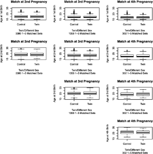
Figure 1: Age at births in 5040 1–5 nonoverlapping matched sets containing 30,240 mothers, specifically 5040 mothers who gave birth to a twin at the indicated pregnancy and 25,200 mothers who had at least one child of each sex by the end of the indicated pregnancy. For 3380 sets matched at the second pregnancy, matching controlled the past, namely age at the first and second births. For 1358 sets matched at the third pregnancy, matching controlled the past, namely age at the first, second and third births. For 302 sets matched at the fourth pregnancy, matching controlled the past, namely age at the first, second, third and fourth births.

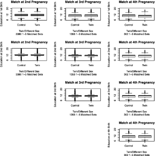
Figure 2: Mother’s education at the time of various births in 5040 1–5 nonoverlapping matched sets containing 30,240 mothers, specifically 5040 mothers who gave birth to a twin at the indicated pregnancy and 25,200 mothers who had at least one child of each sex by at the end of the indicated pregnancy. Each match controls the past, not the future. For graphical display in the boxplots, education is truncated at 6 years despite a few values below that.

Tables 1 and 2 show the comparability of the matched groups separately for the matches at the second, third and fourth pregnancy. Table 1 exhibits perfect balance for categories of race/ethnicity, region of the US and age at the second pregnancy. Moreover, the interactions of these three variables are also exactly balanced.

Table 1: In each matched risk set containing $J=6$ mothers, a mother of a twin at birth $k$ is matched to $J-1=5$ control mothers whose $k$th birth was a single child whose sex was different from one of her previous children. The matching was exact for four age categories, for four race/ethnicity categories and for four regions of the US, and because it was exact, it controlled their interactions. The table displays counts and percents, where the count for controls is always five times the count for twins. Only one column of percents is displayed because the percents in the two groups are identical

	2nd birth			3rd birth			4th birth
Covariate	Twin	Control	%	Twin	Control	%	Twin	Control	%
Age	Mother’s age at her second pregnancy
$\leq 18$	$182$	$910$	$5$	$167$	$835$	$12$	$63$	$315$	21
19–22	$1239$	$6195$	$37$	$677$	$3385$	$50$	$163$	$815$	54
23–25	$1044$	$5220$	$31$	$350$	$1750$	$26$	$63$	$315$	21
$\geq 26$	$915$	$4575$	$27$	$164$	$820$	$12$	$13$	$65$	04
Race/ethnicity	Mother’s race/ethnicity
Black	$505$	$2525$	$15$	$242$	$1210$	$18$	$81$	$405$	27
Hispanic	$87$	$435$	$3$	$63$	$315$	$5$	$11$	$55$	04
White	$2707$	$13\mbox{,}535$	$80$	$1023$	$5115$	$75$	$203$	$1015$	67
Other	$81$	$405$	$2$	$30$	$150$	$2$	$7$	$35$	02
Region	Region of the US
Northeast	$685$	$3425$	$20$	$270$	$1350$	$20$	$60$	$300$	20
South	$1081$	$5405$	$32$	$426$	$2130$	$31$	$100$	$500$	33
Central	$988$	$4940$	$29$	$391$	$1955$	$29$	$93$	$465$	31
West	$626$	$3130$	$19$	$271$	$1355$	$20$	$49$	$245$	16

Table 2: Baseline comparison of 30,240 distinct mothers in $I=5040=3380+1358+302$ nonoverlapping matched sets of $J=6$ mothers, each set containing one mother who gave birth to a twin and $J-1$ control mothers who gave birth to a single child whose sex differed from that of one of her previous children. The table shows age and education of mothers at their various births prior to risk-set matching

	2nd birth		3rd birth		4th birth
Covariate	Twin	Control	Twin	Control	Twin	Control
	Sample size
# of mothers	3380	16,900	1358	6790	302	1510
	Mother’s age in years, mean
At the census	$30.4$	$30.4$	$30.7$	$30.7$	$31.6$	$31.6$
At 1st birth	$20.4$	$20.4$	$19.5$	$19.5$	$18.8$	$18.8$
At 2nd birth	$23.5$	$23.4$	$21.8$	$21.8$	$20.7$	$20.7$
At 3rd birth			$25.1$	$25.1$	$23.5$	$23.4$
At 4th birth					$26.7$	$26.6$
	Mother’s education in years, mean
At 1st birth	$11.9$	$12.0$	$11.4$	$11.4$	$10.8$	$10.9$
At 2nd birth	$12.2$	$12.2$	$11.6$	$11.6$	$11.0$	$11.1$
At 3rd birth			$11.6$	$11.6$	$11.1$	$11.2$
At 4th birth					$11.1$	$11.2$
	Mother’s education at 1st birth, %
High school	$43$	$43$	$42$	$42$	$32$	$33$
Some college	$19$	$19$	$14$	$14$	$15$	$14$
BA or more	$09$	$09$	$05$	$05$	$03$	$03$
	Mother’s education at 2nd birth, %
High school	$47$	$47$	$48$	$48$	$39$	$40$
Some college	$20$	$20$	$15$	$15$	$16$	$15$
BA or more	$11$	$11$	$06$	$06$	$04$	$04$
	Mother’s education at 3rd birth, %
High school			$48$	$48$	$41$	$41$
Some college			$16$	$16$	$16$	$16$
BA or more			$06$	$06$	$05$	$05$
	Mother’s education at 4th birth, %
High school					$41$	$41$
Some college					$16$	$16$
BA or more					$05$	$05$

4 Inference: Tobit effects, proportional effects, sensitivity analysis.

Figure 3 depicts two outcomes recorded on Census day for the 30,240 mothers in 5040 matched sets, each set containing one mother who had a twin at the indicated pregnancy and 5 mothers who had at least one child of each sex at the indicated pregnancy. One outcome is the total number of children recorded on Census day. The other outcome is the work fraction where 0 indicates no work for pay and 1 indicates full time work ($\geq 40$ hours per week). The work fraction is the number of weeks worked in the last year multiplied by the minimum of 40 and the number of hours worked in the last week, and then this product is divided by $40\times 52$ to produce a number between 0 and 1. (A small fraction of mothers worked substantially more than 40 hours in the previous week.)

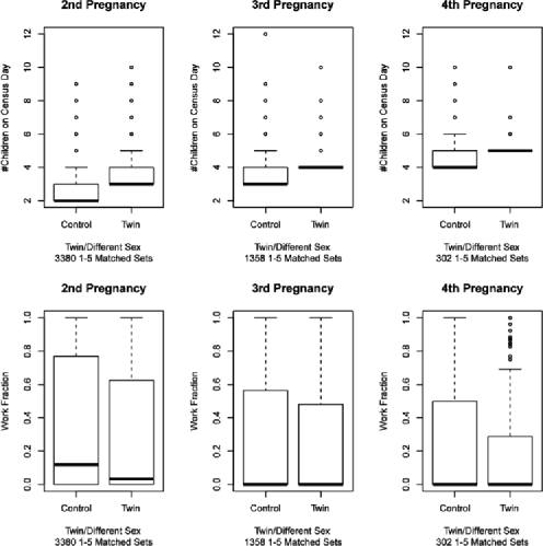
Figure 3: Two outcomes in 5040 1–5 nonoverlapping matched sets containing 30,240 mothers, specifically 5040 mothers who gave birth to a twin at the indicated pregnancy and 25,200 mothers who had at least one child of each sex by at the end of the indicated pregnancy. The upper boxplots indicate the number of children. The lower boxplots indicate the work fraction, defined to be min(hours worked in the previous week, 40)${}\times{}$(weeks worked in the previous year)${}/(40\times 52)$, so a value of 1 is similar to “full time employment.”

In the top half of Figure 3, at the second pregnancy, a twin birth shifted upward by about 1 child the boxplot of number of children. The shift is smaller at the third and fourth pregnancies, where the lower quartile and median increase by 1 child, but the upper quartile is unchanged. Presumably, some mothers pregnant for the third or fourth time intend to have large families and twins did not alter their plans. In the bottom half of Figure 3, mothers of twins worked somewhat less, but the difference in work fraction is not extremely large. Figure 4 displays the information about work fraction in a different format, as a quantile–quantile plot.

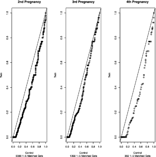
Figure 4: Quantile–quantile plots of work fraction for twins (vertical) and controls (horizontal) with the line of equality. The plot shows that women with twins were more likely to not work, as seen in the horizontal start to the plot, and they worked fewer hours in total, as quantiles fall below the line of equality.

We consider two models for the effect on the fraction worked, $R_{ij}$. One model is a so-called Tobit effect, named for James Tobin, of twin versus different-sex-single-child, $Z_{ij}$. The Tobit effect has $r_{Tij}=\max(0,r_{Cij}-\tau)$ and it reflects the fact that a woman’s workforce participation may decline to zero but not further. For instance, if $\tau=0.1=10\%$, then a mother who would have worked at least $r_{Cij}=10\%$ of full-time without twins would work 10% less with twins, $r_{Tij}=r_{Cij}-10\%$, but a mother who would have worked $r_{Cij}=5\%$ or $r_{Cij}=0\%$ of full-time without twins would not work with twins, $r_{Tij}=0\%$. For the Tobit effect, we draw inferences about $\tau$. If $H_{0}\dvtx\tau=\tau_{0}$ were true, then $\max\{0,R_{ij}-(1-Z_{ij})\tau_{0}\}=r_{Tij}$ does not vary with $Z_{ij}$ and satisfies the null hypothesis of no treatment. Therefore, $H_{0}\dvtx\tau=\tau_{0}$ is the hypothesis of no treatment effect on $\max\{0,R_{ij}-(1-Z_{ij})\tau_{0}\}$ and the confidence interval is obtained in the usual way by inverting the test. In the usual way, the point estimate solves for $\tau$ an estimating equation that equates the test statistic to its null expectation. We use the treated-minus-control mean as the test statistic, but very similar results were obtained using an $M$-estimate with Huber’s weight function trimming at twice the median absolute deviation. See Rosenbaum (2007) and the senmwCI function in the sensitivitymw package in R for computations.

Table 3 displays inferences about $\tau$, the effect of a twin on hours worked or, more precisely, on the work fraction. For $\Gamma=1$, Table 3 displays randomization inferences assuming the differential comparison of twins versus different-single-sex-child is free of bias from unmeasured covariates. For $\Gamma>1$, sensitivity to unmeasured bias is displayed. The point estimate of $\tau$ in the absence of bias is 0.0793 or about 8% reduction in work hours ($0.08\times 40=3.2$ hours per week) for a mother with twins. More precisely, this is an 8% reduction in work fraction or a reduction of 3.2 hours per week for any mother who would work at least 3.2 hours if she did not have twins. The results are insensitive to small biases, say, $\Gamma\leq 1.2$, but are sensitive to moderate bias, $\Gamma=1.25$; however, we do not expect much bias in the differential comparison. As noted in Section 2.3 and Rosenbaum and Silber (2009), in a matched pair, treatment-versus-control comparison, a bias $\Gamma=1.25$ is produced by an unobserved covariate that doubles the odds of treatment and doubles the odds of a positive treatment-minus-control pair difference in outcomes.

Table 3: Inference about the Tobit effect $\tau$. For each $\Gamma$, the sensitivity analysis gives the maximum possible $P$-value testing the null hypothesis of no treatment effect, $H_{0}\dvtx\tau=0$, the minimum one-sided 95% confidence interval and the minimum possible point estimate. Inferences use the mean, but $M$-estimates with Huber weights produced similar results

$\bolds{\Gamma}$	$\bolds{P}$-value	95% CI	Estimate
1.0	$1.6\times 10^{-13}$	$\tau\geq 0.0616$	0.0793
1.1	$2.0\times 10^{-6}$	$\tau\geq 0.0324$	0.0502
1.2	0.0148	$\tau\geq 0.0058$	0.0237
1.25	0.1512

Figure 5 looks at residuals. With $\tau_{0}=0.0793$, Figure 5 plots $\max\{0,R_{ij}-(1-Z_{ij})\tau_{0}\}$. In an infinite sample without bias, this plot would have identical pairs of boxplots if the Tobit effect were correct. Though not identical in pairs, the boxplots are similar, except perhaps at the 4th pregnancy where the sample size is not large. Arguably, the data do not sharply contradict a Tobit effect.

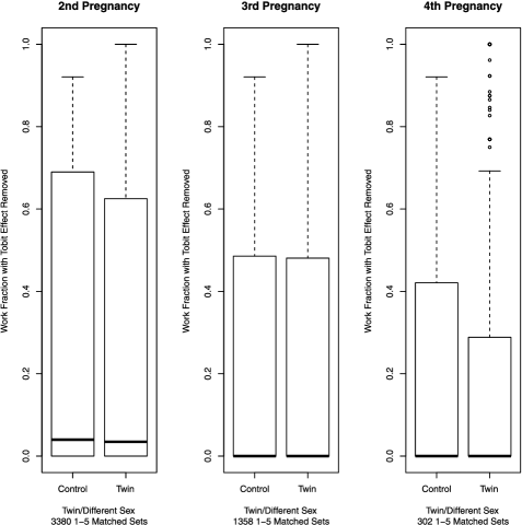
Figure 5: Residuals from the Tobit effect model. The boxplots display $\max\{0,R_{ij}-(1-Z_{ij})\tau_{0}\}$ for $\tau_{0}=0.0793$, the point estimate of $\tau$ at $\Gamma=1$. In an infinitely large sample, if the Tobit model were true with this $\tau$ and $\Gamma$, then the pair of boxplots at each pregnancy would be identical.

The second model related the effect on workforce participation to the effect on the number of children, that is, the two outcomes in Figure 3. Write $D_{ij}$ for the number of children, with $D_{ij}=d_{Tij}$ if $Z_{ij}=1$ and $D_{ij}=d_{Cij}$ if $Z_{ij}=0$. The second model says the effect of twin-versus-different-sex-single child on the workforce outcome is proportional to the effect on the number of children, $r_{Tij}-r_{Cij}=\beta(d_{Tij}-d_{Cij})$. Under this model, $R_{ij}-\beta D_{ij}=r_{Tij}-\beta d_{Tij}=r_{Cij}-\beta d_{Cij}$ does not change with $Z_{ij}$, so (i) the null hypothesis $H_{0}\dvtx\beta=\beta_{0}$ is tested by testing the hypothesis of no effect of the treatment $Z_{ij}$ on $R_{ij}-\beta_{0}D_{ij}$, (ii) a confidence interval for $\beta$ is obtained in the usual way by inverting the test, and (iii) a sensitivity analysis for biased $Z_{ij}$ is conducted in the usual way; see Rosenbaum (1996) and Imbens and Rosenbaum (2005). This model embodies the exclusion restriction in saying that if the twin did not alter the total number of children for mother $ij$, so $d_{Tij}=d_{Cij}$, then it did not alter her workforce participation, $r_{Tij}=r_{Cij}$. For instance, if mother $ij$ had a twin on her second birth, $Z_{ij}=1$, she might have three children, $d_{Tij}=3$, where perhaps she would have had two children if she had had a different-sex-single child at the second birth, $d_{Cij}=2$, so for this mother the twin causes a 1 child increase in her number of children, $d_{Tij}-d_{Cij}=1$, and hence a change in workforce participation of $r_{Tij}-r_{Cij}=\beta(d_{Tij}-d_{Cij})=\beta$. Some other mother, $i^{\prime}j^{\prime}$, might have had three children regardless, $d_{Tij}=d_{Cij}=3$, in which case the twin caused no increase in her number of children, $d_{Tij}-d_{Cij}=0$ so $r_{Tij}-r_{Cij}=0$. Baiocchi et al. (2010) show that randomization inferences (i.e., inferences with $\gamma=\phi_{s}-\phi_{s^{\prime}}=0$) for $\beta$ under the model $r_{Tij}-r_{Cij}=\beta(d_{Tij}-d_{Cij})$ are identical to randomization inferences for the effect ratio, $(\sum_{i=1}^{I}\sum_{j=1}^{J}r_{Tij}-r_{Cij})/(\sum_{i=1}^{I}\sum_{j=1}^{J}d_{Tij}-d_{Cij})$, which is the effect on workforce participation per added child, and this is true whether or not the exclusion restriction holds. For instance, $\beta=-0.1$ would be a 0.1 reduction in the average work fraction per additional child, whether or not $r_{Tij}-r_{Cij}=\beta(d_{Tij}-d_{Cij})$ for each individual $ij$. Without the model $r_{Tij}-r_{Cij}=\beta(d_{Tij}-d_{Cij})$, but with the exclusion restriction, the effect ratio can be interpreted as the average effect on workforce participation per child among mothers who had additional children because of the twin; see Angrist, Imbens and Rubin (1996).

Table 4: Inference about the proportional effect, $\beta$. For each $\Gamma$, the sensitivity analysis gives the maximum possible $P$-value testing the null hypothesis of no treatment effect, $H_{0}\dvtx\beta=0$, the minimum one-sided 95% confidence interval and the minimum possible point estimate. Inferences use the mean, but $M$-estimates with Huber weights produced similar results

$\bolds{\Gamma}$	$\bolds{P}$-value	95% CI	Estimate
1.0	$1.6\times 10^{-13}$	$\beta\leq-0.0365$	$-0.0470$
1.1	$2.0\times 10^{-6}$	$\beta\leq-0.0191$	$-0.0296$
1.2	0.0148	$\beta\leq-0.0034$	$-0.0139$
1.25	0.1512

Table 4 draws inferences about the proportional effect, $\beta$. The test of no treatment effect is the same as in Table 3, so the $P$-values in the two analyses are equally sensitive to unmeasured biases. In the absence of unmeasured bias, $\Gamma=1$, the point estimate of $\beta$ suggests a 5% reduction in the work fraction per additional child. We have been looking at the effects of twins versus the popular mix of children of both sexes. The effects appear to be small.

5 Discussion.

Isolation, as we have defined it, is used in the following situation. One of several treatments may be inflicted upon individuals (or self-inflicted) at certain moments in time. The timing $t$ of treatment may be severely biased by both measured and unmeasured time-varying covariates, but there may be two treatments, $s$ and $s^{\prime}$, such that conditionally given some treatment at $t$, the occurrence of treatment $s$ in lieu of treatment $s^{\prime}$ is close to random. Isolation focuses attention on that brief moment and random aspect by controlling for measured time-dependent covariates using risk-set matching and by removing a generic bias using a differential comparison. Stated precisely, isolation refers to the radical simplification of the conditional probability in (2.3) that occurs when $\phi_{s}=\phi_{s^{\prime}}$; then, the unobserved time dependent covariate $u_{ijt}$ that would bias most comparisons does not bias a risk-set match of treatment $s$ in lieu of $s^{\prime}$. This radical simplification, when it occurs, justifies one very specific analysis: the comparison of matched sets with similar observed histories to time $t$ where some individual received treatment $s$ and the rest received treatment $s^{\prime}$. In the case study, the timing of births is biased by a woman’s plans and aspirations for education, career and family, but conditionally given a birth at time $t$, the occurrence of twins rather than a single birth is largely unaffected by her plans.

In a different study that employed similar reasoning, Nagin and Snodgrass (2013) examined the effects of incarceration on subsequent criminal activity. The substantial difficulty is that judges decide in a thoughtful manner whether to imprison an individual convicted for a crime. When two people are convicted of the same crime, it is far from a random event when one is sent to prison and the other is punished in a different way. Nagin and Snodgrass looked at counties in Pennsylvania in which some judges were much harsher than others, sending many more convicts to prison. Committing a crime is not haphazard, nor is a judge’s decision, but having your case come to trial when judge A rather than judge B is next available is, in most instances, a haphazard event. Nagin and Snodgrass contrasted the subsequent criminal activity of individuals with similar pasts who were tried before harsh judges and those tried before lenient judges in the same county at about the same time, so each convict might have received either judge. They found little or no evidence in support of the widespread belief that harsher judges and harsher sentences reduce the frequency of subsequent rearrest.

A similar strategy is sometimes used in studies of differential effects of biologically different drugs used to treat the same disease. The differential effect may be less confounded than the absolute effect of either drug, particularly if the choice of drug is determined by something haphazard. For example, Brookhart et al. (2006) compared the gastrointestinal toxicity caused by COX-II inhibitors versus NSAIDs by comparing the patients of physicians who usually prescribe one versus those who usually prescribe the other. See also Gibbons et al. (2010) and Ryan et al. (2012).

References

- Angrist and Evans (1998) {barticle}[auto:parserefs-M02] \bauthor\bsnmAngrist, \bfnmJ. D.\binitsJ. D. and \bauthor\bsnmEvans, \bfnmW. N.\binitsW. N. (\byear1998). \btitleChildren and their parent’s labor supply: Evidence from exogenous variation in family size. \bjournalAmer. Econ. Rev. \bvolume88 \bpages450–477. \bptokimsref\endbibitem
- Angrist, Imbens and Rubin (1996) {barticle}[auto:parserefs-M02] \bauthor\bsnmAngrist, \bfnmJ. D.\binitsJ. D., \bauthor\bsnmImbens, \bfnmG. W.\binitsG. W. and \bauthor\bsnmRubin, \bfnmD. B.\binitsD. B. (\byear1996). \btitleIdentification of causal effects using instrumental variables. \bjournalJ. Amer. Statist. Assoc. \bvolume91 \bpages444–455. \bptokimsref\endbibitem
- Anthony et al. (2000) {barticle}[pbm] \bauthor\bsnmAnthony, \bfnmJ. C.\binitsJ. C., \bauthor\bsnmBreitner, \bfnmJ. C.\binitsJ. C., \bauthor\bsnmZandi, \bfnmP. P.\binitsP. P., \bauthor\bsnmMeyer, \bfnmM. R.\binitsM. R., \bauthor\bsnmJurasova, \bfnmI.\binitsI., \bauthor\bsnmNorton, \bfnmM. C.\binitsM. C. and \bauthor\bsnmStone, \bfnmS. V.\binitsS. V. (\byear2000). \btitleReduced prevalence of AD in users of NSAIDs and H2 receptor antagonists: The cache county study. \bjournalNeurology \bvolume54 \bpages2066–2071. \bidissn=0028-3878, pmid=10851364 \bptokimsref\endbibitem
- Apel et al. (2010) {barticle}[auto:parserefs-M02] \bauthor\bsnmApel, \bfnmR.\binitsR., \bauthor\bsnmBlokland, \bfnmA. A. J.\binitsA. A. J., \bauthor\bsnmNieuwbeerta, \bfnmP.\binitsP. and \bauthor\bparticlevan \bsnmSchellen, \bfnmM.\binitsM. (\byear2010). \btitleThe impact of imprisonment on marriage and divorce: A risk-set matching approach. \bjournalJ. Quant. Criminol. \bvolume26 \bpages269–300. \bptokimsref\endbibitem
- Arpino and Aassve (2013) {barticle}[auto:parserefs-M02] \bauthor\bsnmArpino, \bfnmB.\binitsB. and \bauthor\bsnmAassve, \bfnmA.\binitsA. (\byear2013). \btitleEstimating the causal effect of fertility on economic wellbeing: Data requirements, identifying assumptions and estimation methods. \bjournalEmpir. Econ. \bvolume44 \bpages355–385. \bptokimsref\endbibitem
- Baiocchi et al. (2010) {barticle}[mr] \bauthor\bsnmBaiocchi, \bfnmMike\binitsM., \bauthor\bsnmSmall, \bfnmDylan S.\binitsD. S., \bauthor\bsnmLorch, \bfnmScott\binitsS. and \bauthor\bsnmRosenbaum, \bfnmPaul R.\binitsP. R. (\byear2010). \btitleBuilding a stronger instrument in an observational study of perinatal care for premature infants. \bjournalJ. Amer. Statist. Assoc. \bvolume105 \bpages1285–1296. \biddoi=10.1198/jasa.2010.ap09490, issn=0162-1459, mr=2796550 \bptokimsref\endbibitem
- Bound, Jaeger and Baker (1995) {barticle}[auto:parserefs-M02] \bauthor\bsnmBound, \bfnmJ.\binitsJ., \bauthor\bsnmJaeger, \bfnmD. A.\binitsD. A. and \bauthor\bsnmBaker, \bfnmR. M.\binitsR. M. (\byear1995). \btitleProblems with instrumental variables estimation when the correlation between the instruments and the endogenous explanatory variable is weak. \bjournalJ. Amer. Statist. Assoc. \bvolume90 \bpages443–450. \bptokimsref\endbibitem
- Brookhart et al. (2006) {barticle}[pbm] \bauthor\bsnmBrookhart, \bfnmM. Alan\binitsM. A., \bauthor\bsnmWang, \bfnmPhilip S.\binitsP. S., \bauthor\bsnmSolomon, \bfnmDaniel H.\binitsD. H. and \bauthor\bsnmSchneeweiss, \bfnmSebastian\binitsS. (\byear2006). \btitleEvaluating short-term drug effects using a physician-specific prescribing preference as an instrumental variable. \bjournalEpidemiology \bvolume17 \bpages268–275. \biddoi=10.1097/01.ede.0000193606.58671.c5, issn=1044-3983, mid=NIHMS111362, pii=00001648-200605000-00011, pmcid=2715942, pmid=16617275 \bptokimsref\endbibitem
- Campbell (1986) {bincollection}[auto:parserefs-M02] \bauthor\bsnmCampbell, \bfnmD. T.\binitsD. T. (\byear1986). \btitleRelabeling internal and external validity for applied social scientists. In \bbooktitleAdvances in Quasi-Experimental Design and Analysis (\beditor\bfnmW. M. K.\binitsW. M. K. \bsnmTrochim, ed.) \bpages67–77. \bpublisherJossey-Bass, \blocationSan Francisco, CA. \bptokimsref\endbibitem
- Cornfield et al. (1959) {barticle}[pbm] \bauthor\bsnmCornfield, \bfnmJ.\binitsJ., \bauthor\bsnmHaenszel, \bfnmW.\binitsW., \bauthor\bsnmHammond, \bfnmE. C.\binitsE. C., \bauthor\bsnmLilienfeld, \bfnmA. M.\binitsA. M., \bauthor\bsnmShimkin, \bfnmM. B.\binitsM. B. and \bauthor\bsnmWynder, \bfnmE. L.\binitsE. L. (\byear1959). \btitleSmoking and lung cancer: Recent evidence and a discussion of some questions. \bjournalJ. Natl. Cancer Inst. \bvolume22 \bpages173–203. \bidissn=0027-8874, pmid=13621204 \bptnotecheck related \bptokimsref\endbibitem
- Cox (1972) {barticle}[mr] \bauthor\bsnmCox, \bfnmD. R.\binitsD. R. (\byear1972). \btitleRegression models and life-tables. \bjournalJ. R. Stat. Soc. Ser. B Stat. Methodol. \bvolume34 \bpages187–220. \bidissn=0035-9246, mr=0341758 \bptnotecheck related \bptokimsref\endbibitem
- Diprete and Gangl (2004) {barticle}[auto:parserefs-M02] \bauthor\bsnmDiprete, \bfnmT. A.\binitsT. A. and \bauthor\bsnmGangl, \bfnmM.\binitsM. (\byear2004). \btitleAssessing bias in the estimation of causal effects. \bjournalSociolog. Method. \bvolume34 \bpages271–310. \bptokimsref\endbibitem
- Egleston, Scharfstein and MacKenzie (2009) {barticle}[mr] \bauthor\bsnmEgleston, \bfnmBrian L.\binitsB. L., \bauthor\bsnmScharfstein, \bfnmDaniel O.\binitsD. O. and \bauthor\bsnmMacKenzie, \bfnmEllen\binitsE. (\byear2009). \btitleOn estimation of the survivor average causal effect in observational studies when important confounders are missing due to death. \bjournalBiometrics \bvolume65 \bpages497–504. \biddoi=10.1111/j.1541-0420.2008.01111.x, issn=0006-341X, mr=2751473 \bptokimsref\endbibitem
- Gastwirth (1992) {barticle}[auto:parserefs-M02] \bauthor\bsnmGastwirth, \bfnmJ. L.\binitsJ. L. (\byear1992). \btitleMethods for assessing the sensitivity of statistical comparisons used in title VII cases to omitted variables. \bjournalJurimetrics \bvolume33 \bpages19–34. \bptokimsref\endbibitem
- Gibbons et al. (2010) {barticle}[auto:parserefs-M02] \bauthor\bsnmGibbons, \bfnmR. D.\binitsR. D., \bauthor\bsnmAmatya, \bfnmA. K.\binitsA. K., \bauthor\bsnmBrown, \bfnmC. H.\binitsC. H., \bauthor\bsnmHur, \bfnmK.\binitsK., \bauthor\bsnmMarcus, \bfnmS. M.\binitsS. M., \bauthor\bsnmBhaumik, \bfnmD. K.\binitsD. K. and \bauthor\bsnmMann, \bfnmJ.\binitsJ. (\byear2010). \btitlePost-approval drug safety surveillance. \bjournalAnn. Rev. Pub. Health \bvolume31 \bpages419–437. \bptokimsref\endbibitem
- Hansen (2007) {barticle}[auto:parserefs-M02] \bauthor\bsnmHansen, \bfnmB. B.\binitsB. B. (\byear2007). \btitleOptmatch. \bjournalR News \bvolume7 \bpages18–24. \bptokimsref\endbibitem
- Holland (1988) {barticle}[auto:parserefs-M02] \bauthor\bsnmHolland, \bfnmP. W. H.\binitsP. W. H. (\byear1988). \btitleCausal inference, path analysis, and recursive structural equations models. \bjournalSociolog. Method. \bvolume18 \bpages449–484. \bptokimsref\endbibitem
- Hosman, Hansen and Holland (2010) {barticle}[mr] \bauthor\bsnmHosman, \bfnmCarrie A.\binitsC. A., \bauthor\bsnmHansen, \bfnmBen B.\binitsB. B. and \bauthor\bsnmHolland, \bfnmPaul W.\binitsP. W. (\byear2010). \btitleThe sensitivity of linear regression coefficients’ confidence limits to the omission of a confounder. \bjournalAnn. Appl. Stat. \bvolume4 \bpages849–870. \biddoi=10.1214/09-AOAS315, issn=1932-6157, mr=2758424 \bptokimsref\endbibitem
- Hsu and Small (2013) {barticle}[mr] \bauthor\bsnmHsu, \bfnmJesse Y.\binitsJ. Y. and \bauthor\bsnmSmall, \bfnmDylan S.\binitsD. S. (\byear2013). \btitleCalibrating sensitivity analyses to observed covariates in observational studies. \bjournalBiometrics \bvolume69 \bpages803–811. \biddoi=10.1111/biom.12101, issn=0006-341X, mr=3146776 \bptokimsref\endbibitem
- Imai et al. (2011) {barticle}[auto:parserefs-M02] \bauthor\bsnmImai, \bfnmK.\binitsK., \bauthor\bsnmKeele, \bfnmL.\binitsL., \bauthor\bsnmTingley, \bfnmD.\binitsD. and \bauthor\bsnmYamamoto, \bfnmT.\binitsT. (\byear2011). \btitleUnpacking the black box of causality: Learning about causal mechanisms from experimental and observational studies. \bjournalAmer. Polit. Sci. Rev. \bvolume105 \bpages765–789. \bptokimsref\endbibitem
- Imbens and Rosenbaum (2005) {barticle}[mr] \bauthor\bsnmImbens, \bfnmGuido W.\binitsG. W. and \bauthor\bsnmRosenbaum, \bfnmPaul R.\binitsP. R. (\byear2005). \btitleRobust, accurate confidence intervals with a weak instrument: Quarter of birth and education. \bjournalJ. Roy. Statist. Soc. Ser. A \bvolume168 \bpages109–126. \biddoi=10.1111/j.1467-985X.2004.00339.x, issn=0964-1998, mr=2113230 \bptnotecheck year \bptokimsref\endbibitem
- Kennedy et al. (2010) {barticle}[mr] \bauthor\bsnmKennedy, \bfnmEdward H.\binitsE. H., \bauthor\bsnmTaylor, \bfnmJeremy M. G.\binitsJ. M. G., \bauthor\bsnmSchaubel, \bfnmDouglas E.\binitsD. E. and \bauthor\bsnmWilliams, \bfnmScott\binitsS. (\byear2010). \btitleThe effect of salvage therapy on survival in a longitudinal study with treatment by indication. \bjournalStat. Med. \bvolume29 \bpages2569–2580. \biddoi=10.1002/sim.4017, issn=0277-6715, mr=2756944 \bptokimsref\endbibitem
- Li, Propert and Rosenbaum (2001) {barticle}[mr] \bauthor\bsnmLi, \bfnmYunfei Paul\binitsY. P., \bauthor\bsnmPropert, \bfnmKathleen J.\binitsK. J. and \bauthor\bsnmRosenbaum, \bfnmPaul R.\binitsP. R. (\byear2001). \btitleBalanced risk set matching. \bjournalJ. Amer. Statist. Assoc. \bvolume96 \bpages870–882. \biddoi=10.1198/016214501753208573, issn=0162-1459, mr=1946360 \bptokimsref\endbibitem
- Lin, Psaty and Kronmal (1998) {barticle}[pbm] \bauthor\bsnmLin, \bfnmD. Y.\binitsD. Y., \bauthor\bsnmPsaty, \bfnmB. M.\binitsB. M. and \bauthor\bsnmKronmal, \bfnmR. A.\binitsR. A. (\byear1998). \btitleAssessing the sensitivity of regression results to unmeasured confounders in observational studies. \bjournalBiometrics \bvolume54 \bpages948–963. \bidissn=0006-341X, pmid=9750244 \bptokimsref\endbibitem
- Liu, Kuramoto and Stuart (2013) {barticle}[auto:parserefs-M02] \bauthor\bsnmLiu, \bfnmW.\binitsW., \bauthor\bsnmKuramoto, \bfnmJ.\binitsJ. and \bauthor\bsnmStuart, \bfnmE.\binitsE. (\byear2013). \btitleSensitivity analysis for unobserved confounding in nonexperimental prevention research. \bjournalPrev. Sci. \bvolume14 \bpages570–580. \bptokimsref\endbibitem
- Lu (2005) {barticle}[mr] \bauthor\bsnmLu, \bfnmBo\binitsB. (\byear2005). \btitlePropensity score matching with time-dependent covariates. \bjournalBiometrics \bvolume61 \bpages721–728. \biddoi=10.1111/j.1541-0420.2005.00356.x, issn=0006-341X, mr=2196160 \bptokimsref\endbibitem
- Lu et al. (2011) {barticle}[mr] \bauthor\bsnmLu, \bfnmBo\binitsB., \bauthor\bsnmGreevy, \bfnmRobert\binitsR., \bauthor\bsnmXu, \bfnmXinyi\binitsX. and \bauthor\bsnmBeck, \bfnmCole\binitsC. (\byear2011). \btitleOptimal nonbipartite matching and its statistical applications. \bjournalAmer. Statist. \bvolume65 \bpages21–30. \biddoi=10.1198/tast.2011.08294, issn=0003-1305, mr=2899649 \bptokimsref\endbibitem
- Marcus (1997) {barticle}[auto:parserefs-M02] \bauthor\bsnmMarcus, \bfnmS. M.\binitsS. M. (\byear1997). \btitleUsing omitted variable bias to assess uncertainty in the estimation of an AIDS education treatment effect. \bjournalJ. Ed. Behav. Statist. \bvolume22 \bpages193–201. \bptokimsref\endbibitem
- Marcus et al. (2008) {barticle}[auto:parserefs-M02] \bauthor\bsnmMarcus, \bfnmS. M.\binitsS. M., \bauthor\bsnmSiddique, \bfnmJ.\binitsJ., \bauthor\bsnmTen Have, \bfnmT. R.\binitsT. R., \bauthor\bsnmGibbons, \bfnmR. D.\binitsR. D., \bauthor\bsnmStuart, \bfnmE. A.\binitsE. A. and \bauthor\bsnmNormand, \bfnmS. L. T.\binitsS. L. T. (\byear2008). \btitleBalancing treatment comparisons in longitudinal studies. \bjournalPsychiatr. Ann. \bvolume38 \bpages805–811. \bptokimsref\endbibitem
- McCandless, Gustafson and Levy (2007) {barticle}[mr] \bauthor\bsnmMcCandless, \bfnmLawrence C.\binitsL. C., \bauthor\bsnmGustafson, \bfnmPaul\binitsP. and \bauthor\bsnmLevy, \bfnmAdrian\binitsA. (\byear2007). \btitleBayesian sensitivity analysis for unmeasured confounding in observational studies. \bjournalStat. Med. \bvolume26 \bpages2331–2347. \biddoi=10.1002/sim.2711, issn=0277-6715, mr=2368419 \bptokimsref\endbibitem
- Meyer (1995) {barticle}[auto:parserefs-M02] \bauthor\bsnmMeyer, \bfnmB. D.\binitsB. D. (\byear1995). \btitleNatural and quasi-experiments in economics. \bjournalJ. Bus. Econom. Statist. \bvolume13 \bpages151–161. \bptokimsref\endbibitem
- Murray, Loeber and Pardini (2012) {barticle}[auto:parserefs-M02] \bauthor\bsnmMurray, \bfnmJ.\binitsJ., \bauthor\bsnmLoeber, \bfnmR.\binitsR. and \bauthor\bsnmPardini, \bfnmD.\binitsD. (\byear2012). \btitleParental involvement in the criminal justice system and the development of youth theft, marijuana use, depression, and poor academic performance. \bjournalCriminology \bvolume50 \bpages255–302. \bptokimsref\endbibitem
- Nagin and Snodgrass (2013) {barticle}[auto:parserefs-M02] \bauthor\bsnmNagin, \bfnmD. S.\binitsD. S. and \bauthor\bsnmSnodgrass, \bfnmG. M.\binitsG. M. (\byear2013). \btitleThe effect of incarceration on re-offending: Evidence from a natural experiment in Pennsylvania. \bjournalJ. Quant. Criminol. \bvolume29 \bpages601–642. \bptokimsref\endbibitem
- Neyman (1923) {barticle}[mr] \bauthor\bsnmNeyman, \bfnmJ.\binitsJ. (\byear1923). \btitle On the application of probability theory to agricultural experiments. \bjournalStatist. Sci. \bvolume5 \bpages463–464. \bptokimsref\endbibitem
- Nieuwbeerta, Nagin and Blokland (2009) {barticle}[auto:parserefs-M02] \bauthor\bsnmNieuwbeerta, \bfnmP.\binitsP., \bauthor\bsnmNagin, \bfnmD. S.\binitsD. S. and \bauthor\bsnmBlokland, \bfnmA. A. J.\binitsA. A. J. (\byear2009). \btitleAssessing the impack of first-time imprisonment on offender’s subsequent criminal career development: A matched samples comparison. \bjournalJ. Quant. Criminol. \bvolume25 \bpages227–257. \bptokimsref\endbibitem
- Robins, Rotnitzky and Scharfstein (2000) {bincollection}[mr] \bauthor\bsnmRobins, \bfnmJames M.\binitsJ. M., \bauthor\bsnmRotnitzky, \bfnmAndrea\binitsA. and \bauthor\bsnmScharfstein, \bfnmDaniel O.\binitsD. O. (\byear2000). \btitleSensitivity analysis for selection bias and unmeasured confounding in missing data and causal inference models. In \bbooktitleStatistical Models in Epidemiology, the Environment, and Clinical Trials (Minneapolis, MN, 1997) (\beditor\binitsE.\bfnmE. \bsnmHalloran and \beditor\binitsD.\bfnmD. \bsnmBerry, eds.). \bseriesIMA Vol. Math. Appl. \bvolume116 \bpages1–94. \bpublisherSpringer, \blocationNew York. \biddoi=10.1007/978-1-4612-1284-3_1, mr=1731681 \bptnotecheck year \bptokimsref\endbibitem
- Rosenbaum (1984) {barticle}[auto:parserefs-M02] \bauthor\bsnmRosenbaum, \bfnmP. R.\binitsP. R. (\byear1984). \btitleThe consequences of adjustment for a concomitant variable that has been affected by the treatment. \bjournalJ. Roy. Statist. Soc. Ser. A \bvolume147 \bpages656–666. \bptokimsref\endbibitem
- Rosenbaum (1987) {barticle}[auto:parserefs-M02] \bauthor\bsnmRosenbaum, \bfnmP. R.\binitsP. R. (\byear1987). \btitleSensitivity analysis for certain permutation tests in matched observational studies. \bjournalBiometrika \bvolume74 \bpages13–26. \bptokimsref\endbibitem
- Rosenbaum (1996) {barticle}[auto:parserefs-M02] \bauthor\bsnmRosenbaum, \bfnmP. R.\binitsP. R. (\byear1996). \btitleComment. \bjournalJ. Amer. Statist. Assoc. \bvolume91 \bpages465–468. \bptokimsref\endbibitem
- Rosenbaum (2006) {barticle}[mr] \bauthor\bsnmRosenbaum, \bfnmPaul R.\binitsP. R. (\byear2006). \btitleDifferential effects and generic biases in observational studies. \bjournalBiometrika \bvolume93 \bpages573–586. \biddoi=10.1093/biomet/93.3.573, issn=0006-3444, mr=2261443 \bptokimsref\endbibitem
- Rosenbaum (2007) {barticle}[mr] \bauthor\bsnmRosenbaum, \bfnmPaul R.\binitsP. R. (\byear2007). \btitleSensitivity analysis for -estimates, tests, and confidence intervals in matched observational studies. \bjournalBiometrics \bvolume63 \bpages456–464. \biddoi=10.1111/j.1541-0420.2006.00717.x, issn=0006-341X, mr=2370804 \bptokimsref\endbibitem
- Rosenbaum (2010) {bbook}[mr] \bauthor\bsnmRosenbaum, \bfnmPaul R.\binitsP. R. (\byear2010). \btitleDesign of Observational Studies. \bpublisherSpringer, \blocationNew York. \biddoi=10.1007/978-1-4419-1213-8, mr=2561612 \bptokimsref\endbibitem
- Rosenbaum (2013a) {barticle}[auto:parserefs-M02] \bauthor\bsnmRosenbaum, \bfnmP. R.\binitsP. R. (\byear2013a). \btitleUsing differential comparisons in observational studies. \bjournalChance \bvolume26 \bpages18–25. \bptokimsref\endbibitem
- Rosenbaum (2013b) {barticle}[mr] \bauthor\bsnmRosenbaum, \bfnmPaul R.\binitsP. R. (\byear2013b). \btitleImpact of multiple matched controls on design sensitivity in observational studies. \bjournalBiometrics \bvolume69 \bpages118–127. \biddoi=10.1111/j.1541-0420.2012.01821.x, issn=0006-341X, mr=3058058 \bptokimsref\endbibitem
- Rosenbaum and Silber (2009) {barticle}[mr] \bauthor\bsnmRosenbaum, \bfnmPaul R.\binitsP. R. and \bauthor\bsnmSilber, \bfnmJeffrey H.\binitsJ. H. (\byear2009). \btitleAmplification of sensitivity analysis in matched observational studies. \bjournalJ. Amer. Statist. Assoc. \bvolume104 \bpages1398–1405. \biddoi=10.1198/jasa.2009.tm08470, issn=0162-1459, mr=2750570 \bptokimsref\endbibitem
- Rubin (1974) {barticle}[auto:parserefs-M02] \bauthor\bsnmRubin, \bfnmD. B.\binitsD. B. (\byear1974). \btitleEstimating causal effects of treatments in randomized and nonrandomized studies. \bjournalJ. Educ. Psych. \bvolume66 \bpages688–701. \bptokimsref\endbibitem
- Rutter (2007) {barticle}[auto:parserefs-M02] \bauthor\bsnmRutter, \bfnmM.\binitsM. (\byear2007). \btitleProceeding from observed correlation to causal inference: The use of natural experiments. \bjournalPerspect. Psychol. Sci. \bvolume2 \bpages377–395. \bptokimsref\endbibitem
- Ryan et al. (2012) {barticle}[mr] \bauthor\bsnmRyan, \bfnmPatrick B.\binitsP. B., \bauthor\bsnmMadigan, \bfnmDavid\binitsD., \bauthor\bsnmStang, \bfnmPaul E.\binitsP. E., \bauthor\bsnmOverhage, \bfnmJ. Marc\binitsJ. M., \bauthor\bsnmRacoosin, \bfnmJudith A.\binitsJ. A. and \bauthor\bsnmHartzema, \bfnmAbraham G.\binitsA. G. (\byear2012). \btitleEmpirical assessment of methods for risk identification in healthcare data: Results from the experiments of the observational medical outcomes partnership. \bjournalStat. Med. \bvolume31 \bpages4401–4415. \biddoi=10.1002/sim.5620, issn=0277-6715, mr=3040089 \bptokimsref\endbibitem
- Sekhon and Titiunik (2012) {barticle}[auto:parserefs-M02] \bauthor\bsnmSekhon, \bfnmJ. S.\binitsJ. S. and \bauthor\bsnmTitiunik, \bfnmR.\binitsR. (\byear2012). \btitleWhen natural experiments are neither natural nor experiments. \bjournalAmer. Polit. Sci. Rev. \bvolume106 \bpages35–57. \bptokimsref\endbibitem
- Small (2007) {barticle}[mr] \bauthor\bsnmSmall, \bfnmDylan S.\binitsD. S. (\byear2007). \btitleSensitivity analysis for instrumental variables regression with overidentifying restrictions. \bjournalJ. Amer. Statist. Assoc. \bvolume102 \bpages1049–1058. \biddoi=10.1198/016214507000000608, issn=0162-1459, mr=2411664 \bptokimsref\endbibitem
- Small and Rosenbaum (2008) {barticle}[mr] \bauthor\bsnmSmall, \bfnmDylan S.\binitsD. S. and \bauthor\bsnmRosenbaum, \bfnmPaul R.\binitsP. R. (\byear2008). \btitleWar and wages: The strength of instrumental variables and their sensitivity to unobserved biases. \bjournalJ. Amer. Statist. Assoc. \bvolume103 \bpages924–933. \biddoi=10.1198/016214507000001247, issn=0162-1459, mr=2528819 \bptokimsref\endbibitem
- Stuart (2010) {barticle}[mr] \bauthor\bsnmStuart, \bfnmElizabeth A.\binitsE. A. (\byear2010). \btitleMatching methods for causal inference: A review and a look forward. \bjournalStatist. Sci. \bvolume25 \bpages1–21. \biddoi=10.1214/09-STS313, issn=0883-4237, mr=2741812 \bptokimsref\endbibitem
- Susser (1973) {bbook}[auto:parserefs-M02] \bauthor\bsnmSusser, \bfnmM.\binitsM. (\byear1973). \btitleCausal Thinking in the Health Sciences. \bpublisherOxford, \blocationNew York. \bptokimsref\endbibitem
- Susser (1981) {barticle}[auto:parserefs-M02] \bauthor\bsnmSusser, \bfnmM.\binitsM. (\byear1981). \btitlePrenatal nutrition, birthweight, and psychological development: An overview of experiments, quasi-experiments, and natural experiments in the past decade. \bjournalAmer. J. Clin. Nutrition \bvolume34 \bpages784–803. \bptokimsref\endbibitem
- Vandenbroucke (2004) {barticle}[pbm] \bauthor\bsnmVandenbroucke, \bfnmJan P.\binitsJ. P. (\byear2004). \btitleWhen are observational studies as credible as randomised trials? \bjournalLancet \bvolume363 \bpages1728–1731. \biddoi=10.1016/S0140-6736(04)16261-2, issn=1474-547X, pii=S0140-6736(04)16261-2, pmid=15158638 \bptokimsref\endbibitem
- van der Laan and Robins (2003) {bbook}[mr] \bauthor\bsnmvan der Laan, \bfnmMark J.\binitsM. J. and \bauthor\bsnmRobins, \bfnmJames M.\binitsJ. M. (\byear2003). \btitleUnified Methods for Censored Longitudinal Data and Causality. \bseriesSpringer Series in Statistics. \bpublisherSpringer, \blocationNew York. \biddoi=10.1007/978-0-387-21700-0, mr=1958123 \bptokimsref\endbibitem
- Wang and Krieger (2006) {barticle}[mr] \bauthor\bsnmWang, \bfnmLiansheng\binitsL. and \bauthor\bsnmKrieger, \bfnmAbba M.\binitsA. M. (\byear2006). \btitleCausal conclusions are most sensitive to unobserved binary covariates. \bjournalStat. Med. \bvolume25 \bpages2257–2271. \biddoi=10.1002/sim.2344, issn=0277-6715, mr=2240099 \bptokimsref\endbibitem
- Wildeman, Schnittker and Turney (2012) {barticle}[auto:parserefs-M02] \bauthor\bsnmWildeman, \bfnmC.\binitsC., \bauthor\bsnmSchnittker, \bfnmJ.\binitsJ. and \bauthor\bsnmTurney, \bfnmK.\binitsK. (\byear2012). \btitleDespair by association? \bjournalAmer. Sociol. Rev. \bvolume77 \bpages216–243. \bptokimsref\endbibitem
- Yu and Gastwirth (2005) {barticle}[auto:parserefs-M02] \bauthor\bsnmYu, \bfnmB. B.\binitsB. B. and \bauthor\bsnmGastwirth, \bfnmJ. L.\binitsJ. L. (\byear2005). \btitleSensitivity analysis for trend tests: Application to the risk of radiation exposure. \bjournalBiostatistics \bvolume6 \bpages201–209. \bptokimsref\endbibitem
- Zubizarreta (2012) {barticle}[mr] \bauthor\bsnmZubizarreta, \bfnmJosé R.\binitsJ. R. (\byear2012). \btitleUsing mixed integer programming for matching in an observational study of kidney failure after surgery. \bjournalJ. Amer. Statist. Assoc. \bvolume107 \bpages1360–1371. \biddoi=10.1080/01621459.2012.703874, issn=0162-1459, mr=3036400 \bptokimsref\endbibitem
- Zubizarreta et al. (2013) {barticle}[mr] \bauthor\bsnmZubizarreta, \bfnmJosé R.\binitsJ. R., \bauthor\bsnmSmall, \bfnmDylan S.\binitsD. S., \bauthor\bsnmGoyal, \bfnmNeera K.\binitsN. K., \bauthor\bsnmLorch, \bfnmScott\binitsS. and \bauthor\bsnmRosenbaum, \bfnmPaul R.\binitsP. R. (\byear2013). \btitleStronger instruments via integer programming in an observational study of late preterm birth outcomes. \bjournalAnn. Appl. Stat. \bvolume7 \bpages25–50. \biddoi=10.1214/12-AOAS582, issn=1932-6157, mr=3086409 \bptokimsref\endbibitem