Structure Learning in Bayesian Networks of Moderate Size by Efficient Sampling

Abstract

We study the Bayesian model averaging approach to learning Bayesian network structures (DAGs) from data. We develop new algorithms including the first algorithm that is able to efficiently sample DAGs according to the exact structure posterior. The DAG samples can then be used to construct estimators for the posterior of any feature. We theoretically prove good properties of our estimators and empirically show that our estimators considerably outperform the estimators from the previous state-of-the-art methods.

Keywords: Bayesian Networks, Structure Learning, Bayesian Model Averaging, Sampling

1 Introduction

Bayesian networks are graphical representations of multivariate joint probability distributions and have been widely used in various data mining tasks for probabilistic inference and causal modeling (Pearl, 2000; Spirtes et al., 2001). The core of a Bayesian network (BN) representation is its Bayesian network structure. A Bayesian network structure is a DAG (directed acyclic graph) whose nodes represent the random variables $X_{1},X_{2},\cdots,X_{n}$ in the problem domain and whose edges correspond to the direct probabilistic dependencies. Semantically, a Bayesian network structure $G$ encodes a set of conditional independence assumptions: for each variable (node) $X_{i}$, $X_{i}$ is conditionally independent of its non-descendants given its parents. With the above semantics, a Bayesian network structure provides a compact representation for joint distributions and supports efficient algorithms for answering probabilistic queries. Furthermore, with its semantics, a Bayesian network structure can often provide a deep insight into the problem domain and open the door to the cause-and-effect analysis.

In the last two decades, there have been a large number of researches focusing on the problem of learning Bayesian network structure(s) from the data. These researches deal with a common real situation where the underlying Bayesian network is typically unknown so that it has to be learned from the observed data. One motivation for the structure learning is to use the learned structure for inference or decision making. For example, we can use the learned model to predict or classify a new instance of data. Another structure-learning motivation, which is more closely related to the semantics of Bayesian network structures, is for discovering the structure of the problem domain. For example, in the context of biological expression data, the discovery of the causal and dependence relation among different genes is often of primary interests. With the semantics of a Bayesian network structure $G$, the existence of an edge from node $X$ to node $Y$ in $G$ can be interpreted as the fact that variable $X$ directly influences variable $Y$; and the existence of a directed path from node $X$ to node $Y$ can be interpreted as the fact that $X$ eventually influences $Y$. Furthermore, under certain assumptions (Heckerman et al., 1999; Spirtes et al., 2001), the existence of a directed path from node $X$ to node $Y$ indicates that $X$ causes $Y$. Thus, with the learned Bayesian network structure, we can answer interesting questions such as whether gene $X$ controls gene $Y$ which in turn controls gene $Z$ by examining whether there is a directed path from node $X$ via node $Y$ to node $Z$ in the learned structure. Just as mentioned by Friedman and Koller (2003), the extraction of these kinds of interesting structural features is often the primary goal in the discovery task.

There are several general approaches to learning BN structures. One approach is to treat it as a model selection problem. This approach defines a scoring criterion that measures how well a BN structure (DAG) fits the data and finds the DAG (or a set of equivalent DAGs) with the optimal score (Silander and Myllymaki, 2006; Jaakkola et al., 2010; Yuan et al., 2011; Malone et al., 2011a, b; Cussens, 2011; Yuan and Malone, 2012; Malone and Yuan, 2013; Cussens and Bartlett, 2013; Yuan and Malone, 2013). (In Bayesian approach, the score of a DAG $G$ is simply the posterior $p(G|D)$ of $G$ given data $D$.) However, when the data size is small relative to the number of variables, the posterior $p(G|D)$ often gives significant support to a number of DAGs, and using a single maximum-a-posteriori (MAP) model could lead to unwarranted conclusions (Friedman and Koller, 2003). It is therefore desirable to use the Bayesian model averaging approach by which the posterior probability of any feature of interest is computed by averaging over all the possible DAGs (Heckerman et al., 1999).

Bayesian model averaging is, however, computationally challenging because the number of possible network structures is between $2^{n(n-1)/2}$ and $n!2^{n(n-1)/2}$, super-exponential in the number of variables $n$. Tractable algorithms have been developed for special cases of averaging over trees (Meila and Jaakkola, 2006) and averaging over DAGs given a node ordering (Dash and Cooper, 2004). Since 2004, dynamic programming (DP) algorithms have been developed for computing exact posterior probabilities of structural features such as edges or subnetworks (Koivisto and Sood, 2004; Koivisto, 2006; Tian and He, 2009). These algorithms have exponential time and space complexity and are capable of handling Bayesian networks of moderate size with up to around $25$ variables (mainly due to their space cost $O(n2^{n})$). A big limitation of these algorithms is that they can only compute posteriors of modular features such as an edge but can not compute non-modular features such as a path (“is there a path from node $X$ to node $Y$”), a combined path (“is there a path from node $X$ via node $Y$ to node $Z$” or “is there a path from node $X$ to node $Y$ and no path from node $X$ to node $Z$”), or a limited-length path (“is there a path of length at most 3 from node $X$ to node $Y$”). Recently, Parviainen and Koivisto (2011) have developed a DP algorithm that can compute the exact posterior probability of a path feature under a certain assumption. (The assumption, called order-modular assumption, will be discussed in details soon.) This DP algorithm has (even higher) exponential time and space complexity and can only handle a Bayesian network with fewer than $20$ variables (mainly due to its space cost $O(3^{n})$). Since this DP algorithm can only deal with a path feature, all the other non-modular features (such as a combined path) which various users would be interested in for their corresponding problems still can not be computed by any DP algorithm proposed so far. Note that generally the posterior $p(f|D)$ of a combined feature $f=(f_{1},f_{2},\ldots,f_{J})$ can not be obtained only from the posterior of each individual feature $p(f_{j}|D)$ ($j\in\{1,2,\ldots,J\}$) because the independence among these features does not hold generally. Actually, by comparing $p(f_{2}|f_{1},D)$ with $p(f_{2}|D)$, a user can know the effect of the feature $f_{1}$ upon the feature $f_{2}$; but to obtain $p(f_{2}|f_{1},D)$ $(=p(f_{1},f_{2}|D)/p(f_{1}|D))$, the user typically needs to obtain $p(f_{1},f_{2}|D)$ first. Another limitation of all these DP algorithms is that it is very expensive for them to perform data prediction tasks. They can compute the exact posterior of a new observational data case $p(x|D)$ but the algorithms have to be re-run for each new data case $x$.

One solution to computing the posterior of an arbitrary non-modular feature is drawing DAG samples $\{G_{1},\ldots,G_{T}\}$ from the posterior $p(G|D)$, which can then be used to approximate the full Bayesian model averaging by estimating the posterior of an arbitrary feature $f$ as $p(f|D)$ $\approx\frac{1}{T}\sum_{i=1}^{T}f(G_{i})$, or the posterior predictive distribution as $p(x|D)$ $\approx\frac{1}{T}\sum_{i=1}^{T}p(x|G_{i})$. A number of algorithms have been developed for drawing sample DAGs using the bootstrap technique (Friedman et al., 1999) or the Markov Chain Monte Carlo (MCMC) techniques (Madigan and York, 1995; Friedman and Koller, 2003; Eaton and Murphy, 2007; Grzegorczyk and Husmeier, 2008; Niinimaki et al., 2011; Niinimaki and Koivisto, 2013). Madigan and York (1995) developed the Structure MCMC algorithm that uses the Metropolis-Hastings algorithm in the space of DAGs. Friedman and Koller (2003) developed the Order MCMC procedure that operates in the space of orders. The Order MCMC was shown to be able to considerably improve over the Structure MCMC the mixing and convergence of the Markov chain and to outperform the bootstrap approach of Friedman et al. (1999) as well. Eaton and Murphy (2007) developed the Hybrid MCMC method (i.e., DP+MCMC method) that first runs the DP algorithm of Koivisto (2006) to develop a global proposal distribution and then runs the MCMC phase in the DAG space. Their experiments showed that the Hybrid MCMC converged faster than both the Structure MCMC and the Order MCMC so that the Hybrid MCMC resulted in more accurate structure learning performance. An improved MCMC algorithm (often denoted as REV-MCMC) traversing in the DAG space with the addition of a new edge reversal move was developed by Grzegorczyk and Husmeier (2008) and was shown to be superior to the Structure MCMC and nearly as efficient as the Order MCMC in the mixing and convergence. Recently, Niinimaki et al. (2011) have proposed the Partial Order MCMC method which operates in the space of partial orders. The Partial Order MCMC includes the Order MCMC as its special case (by setting the parameter bucket size $b$ to be 1) and has been shown to be superior to the Order MCMC in terms of the mixing and the structural learning performance when a more appropriate bucket size $b>1$ is set. One common drawback of these MCMC algorithms is that there is no guarantee on the quality of the approximation in finite runs. The approach to approximating full Bayesian model averaging using the $K$-best Bayesian network structures was studied by Tian et al. (2010) and was shown to be competitive with the Hybrid MCMC.

Several of these state-of-the-art algorithms work in the order space, including the exact algorithms (Koivisto and Sood, 2004; Koivisto, 2006; Parviainen and Koivisto, 2011) and the approximate algorithms: the Order MCMC (Friedman and Koller, 2003) and the Partial Order MCMC (Niinimaki et al., 2011). They all assume a special form of the structure prior, termed as order-modular prior (Friedman and Koller, 2003; Koivisto and Sood, 2004), for computational convenience. (Please refer to the beginning of Section 2.1 for the definition of the order-modular prior.) However, the assumption of order-modular prior has the consequence that the corresponding prior $p(G)$ cannot represent some desirable priors such as a uniform prior over the DAG space; and the computed posterior probabilities are biased since a DAG that has a larger number of topological orders will be assigned a larger prior probability. Whether a computed posterior with the bias from the order-modular prior is inferior to its counterpart without such a bias depends on the application scenario and is beyond the scope of this paper. For the detailed discussion about this issue, please see the related papers (Friedman and Koller, 2003; Grzegorczyk and Husmeier, 2008; Parviainen and Koivisto, 2011). One method that helps the Order MCMC (Friedman and Koller, 2003) to correct this bias was proposed by Ellis and Wong (2008).

In this paper, first we develop a new algorithm that uses the results of the DP algorithm of Koivisto and Sood (2004) to efficiently sample orders according to the exact order posterior under the assumption of order-modular prior. Next, we develop a time-saving strategy for the process of sampling DAGs consistent with given orders. (Such a DAG-sampling process is based on sampling parents for each node as described by Friedman and Koller (2003) by assuming a bounded node in-degree.) The resulting algorithm (called DDS) is the first algorithm that is able to sample DAGs according to the exact DAG posterior with the same order-modular prior assumption. We empirically show that our DDS algorithm is both considerably more accurate and considerably more efficient than the Order MCMC and the Partial Order MCMC when $n$ is moderate so that our DDS algorithm is applicable. Moreover, the estimator based on our DDS algorithm has several desirable properties; for example, unlike the existing MCMC algorithms, the quality of our estimator can be guaranteed by controlling the number of DAGs sampled by our DDS algorithm. The main application of our DDS algorithm is to address the limitation of the exact DP algorithms (Koivisto and Sood, 2004; Koivisto, 2006; Parviainen and Koivisto, 2011) (whose usage is restricted to modular features or path features) in order to estimate the posteriors of various non-modular features arbitrarily specified by users. Additionally our DDS algorithm can also be used to efficiently perform data prediction tasks in estimating $p(x|D)$ for a large number of data cases (while the exact DP algorithm has to be re-run for each case $x$). Finally, we develop an algorithm (called IW-DDS) to correct the bias (due to the order-modular prior) in the DDS algorithm by extending the idea of Ellis and Wong (2008). We theoretically prove that the estimator based on our IW-DDS has several desirable properties; then we empirically show that our estimator is superior to the estimators based on the Hybrid MCMC method (Eaton and Murphy, 2007) and the $K$-best algorithm (Tian et al., 2010), two state-of-the-art algorithms that can estimate the posterior of any feature without the order-modular prior assumption. Analogously, our IW-DDS algorithm mainly addresses the limitation of the exact DP algorithm of Tian and He (2009) (whose usage is restricted to modular features) in order to estimate the posteriors of arbitrary non-modular features and can additionally be used to efficiently perform data prediction tasks when an application situation prefers to avoid the bias from order-modular prior.

The rest of the paper is organized as follows. In Section 2 we briefly review the Bayesian approach to learning Bayesian networks from data, the related DP algorithms (Koivisto and Sood, 2004; Koivisto, 2006) and the Order MCMC algorithm (Friedman and Koller, 2003). In Section 3 we present our order sampling algorithm, DDS algorithm, and IW-DDS algorithm; and prove good properties of the estimators based on our algorithms. We empirically demonstrate the advantages of our algorithms in Section 4. Section 5 concludes the paper. Finally, Appendix A provides the proofs of all the conclusions including the propositions, theorems and corollary referenced in the paper.

2 Bayesian Learning of Bayesian Networks

A Bayesian network is a DAG $G$ that encodes a joint probability distribution over a set $X=\{X_{1},\ldots,X_{n}\}$ of random variables with each node of the DAG representing a variable in $X$. For convenience we typically work on the index set $V=\{1,\ldots,n\}$ and represent a variable $X_{i}$ by its index $i$. We use $X_{Pa_{i}}\subseteq X$ to represent the parent set of $X_{i}$ in a DAG $G$ and use $Pa_{i}\subseteq V$ to represent the corresponding index set. (A pair $(i,Pa_{i})$ is often called a family.) Thus, a DAG $G$ can be represented as a vector $(Pa_{1},\ldots,Pa_{n})$.

Assume that we are given a training data set $D=\{x^{1},x^{2},\ldots,x^{m}\}$, where each $x^{i}$ is a particular instantiation over the set of variables $X$. We only consider situations where the data are complete, that is, every variable in $X$ is assigned a value. In the Bayesian approach to learning Bayesian networks from the training data $D$, we compute the posterior probability of a DAG $G$ as

$$p(G|D)=\frac{p(D|G)p(G)}{p(D)}=\frac{p(D|G)p(G)}{\sum_{G}p(D|G)p(G)}.$$

Assuming global and local parameter independence, and parameter modularity, $p(D|G)$ can be decomposed into a product of local marginal likelihoods (often called local scores) as (Cooper and Herskovits, 1992; Heckerman et al., 1995)

$$p(D|G)=\prod_{i=1}^{n}p(X_{i}|X_{Pa_{i}}:D):=\prod_{i=1}^{n}score_{i}(Pa_{i}:D),$$ (1)

where, with appropriate parameter priors, $score_{i}(Pa_{i}:D)$ (the local score for a family $(i,Pa_{i})$) has a closed form solution. In this paper we will assume that these local scores can be computed efficiently from data. The standard assumption for structure prior $p(G)$ is structure-modular prior (Friedman and Koller, 2003):

$$p(G)=\prod_{i=1}^{n}p_{i}(Pa_{i}),$$ (2)

where $p_{i}$ is some nonnegative function over the subsets of $V-\{i\}$.

Combing Eq. (1) and Eq. (2), we have

$$p_{\nprec}(G,D)=p(D|G)p(G)=\prod_{i=1}^{n}score_{i}(Pa_{i}:D)p_{i}(Pa_{i}).$$ (3)

Note that the subscript $\nprec$ is intentionally added by us to mean that the corresponding probability is the one obtained without order-modular prior assumption. This is different from the probability computed with order-modular prior assumption, which will be marked by the subscript $\prec$ for the distinction.

We can compute the posterior probability of any hypothesis of interest by averaging over all the possible DAGs. For example, we are often interested in computing the posteriors of structural features. Let $f$ be a structural feature represented by an indicator function such that $f(G)$ is 1 if the feature is present in $G$ and 0 otherwise. By the full Bayesian model averaging, we have the posterior of $f$ as

$$p(f|D)=\sum_{G}f(G)p(G|D).$$ (4)

Note that $p_{\nprec}(f|D)$ will be obtained if $p(G|D)$ in Eq. (4) is $p_{\nprec}(G|D)$; $p_{\prec}(f|D)$ will be obtained if $p(G|D)$ in Eq. (4) is $p_{\prec}(G|D)$. This difference is the key to understanding the bias issue which will be described in details later.

Since summing over all the possible DAGs is generally infeasible for any problem with $n>6$ using a contemporary computer, one approach to computing the posterior of $f$ is to draw DAG samples $\{G_{1},\ldots,G_{T}\}$ from the posterior $p_{\nprec}(G|D)$ or $p_{\prec}(G|D)$, which can then be used to estimate the posterior $p_{\nprec}(f|D)$ or $p_{\prec}(f|D)$ as

$$\hat{p}(f|D)=\frac{1}{T}\sum_{i=1}^{T}f(G_{i}).$$ (5)

2.1 The DP Algorithms

The DP algorithms (Koivisto and Sood, 2004; Koivisto, 2006) work in the order space rather than the DAG space. We define an order $\prec$ of variables as a total order (a linear order) on $V$ represented as a vector $(U_{1},\ldots,U_{n})$, where $U_{i}$ is the set of predecessors of $i$ in the order $\prec$. To be more clear we may use $U^{\prec}_{i}$. We say that a DAG $G=(Pa_{1},\ldots,Pa_{n})$ is consistent with an order $(U_{1},\ldots,U_{n})$, denoted by $G\subseteq\prec$, if $Pa_{i}\subseteq U_{i}$ for each $i$. If $S$ is a subset of $V$, we let $\mathcal{L}(S)$ denote the set of linear orders on $S$. In the following we will largely follow the notation from Koivisto (2006).

The algorithms working in the order space assume order-modular prior defined as follows: if $G$ is consistent with $\prec$, then

$$p(\prec,G)=\prod_{i=1}^{n}q_{i}(U_{i})\rho_{i}(Pa_{i}),$$ (6)

where each $q_{i}$ and $\rho_{i}$ is some function from the subsets of $V-\{i\}$ to the nonnegative real numbers. (If $G$ is not consistent with $\prec$, then $p(\prec,G)=0$.)

A modular feature is defined as:

$$f(G)=\prod_{i=1}^{n}f_{i}(Pa_{i}),$$

where $f_{i}(Pa_{i})$ is an indicator function returning a $0/1$ value. For example, an edge feature $j\rightarrow i$ can be represented by setting $f_{i}(Pa_{i})=1$ if and only if $j\in Pa_{i}$ and setting $f_{l}(Pa_{l})=1$ for all $l\neq i$.

With the order-modular prior, we are interested in the posterior $p_{\prec}(f|D)=p_{\prec}(f,D)/p_{\prec}(D)$. $p_{\prec}(f|D)$ can be obtained if the joint probability $p_{\prec}(f,D)$ can be computed (since $p_{\prec}(D)$ $=p_{\prec}(f\equiv 1,D)$ where $f\equiv 1$, meaning that $f$ always equals 1, can be easily achieved by setting each $f_{i}(Pa_{i})$ to be the constant 1). Koivisto and Sood (2004) show that

$$p(f,\prec,D) =\prod_{i=1}^{n}\alpha_{i}(U^{\prec}_{i}),$$ (7)

and

$$p_{\prec}(f,D) =\sum_{\prec}\prod_{i=1}^{n}\alpha_{i}(U^{\prec}_{i}),$$ (8)

where the function $\alpha_{i}$ is defined for each $i\in V$ and each $S\subseteq V-\{i\}$ as

$$\alpha_{i}(S)=q_{i}(S)\sum_{Pa_{i}\subseteq S}\beta_{i}(Pa_{i}),$$

in which the function $\beta_{i}$ is defined for each $i\in V$ and each $Pa_{i}\subseteq V-\{i\}$ as

$$\beta_{i}(Pa_{i})=f_{i}(Pa_{i})\rho_{i}(Pa_{i})score_{i}(Pa_{i}:D).$$

Accordingly, the DP algorithm of Koivisto and Sood (2004) consists of the following three steps. The first step computes $\beta_{i}(Pa_{i})$ for each $i\in V$ and each $Pa_{i}\subseteq V-\{i\}$. The time complexity of this step is $O(n^{k+1}C(m))$ under the assumption of the maximum in-degree $k$, where $n$ is the number of variables, and $C(m)$ is the cost of computing a single local marginal likelihood $score_{i}(Pa_{i}:D)$ for $m$ data instances. The second step computes $\alpha_{i}(S)$ for each $i\in V$ and each $S\subseteq V-\{i\}$. With the assumed maximum in-degree $k$, this step takes $O(kn2^{n})$ time by using the truncated Möbius transform technique (Koivisto and Sood, 2004) which is extended from the standard fast Möbius transform algorithm (Kennes and Smets, 1991). The third step computes $p_{\prec}(f,D)$ by defining the following function (called forward contribution) for each $S\subseteq V$:

$$L(S)=\sum_{\prec\in\mathcal{L}(S)}\prod_{i\in S}\alpha_{i}(U^{\prec}_{i}),$$ (9)

where $U^{\prec}_{i}$ is the set of variables in $S$ ahead of $i$ in the order $\prec\in\mathcal{L}(S)$. It can be shown that for every $S\subseteq V$ the corresponding $L(S)$ can be computed recursively using the DP technique according to the following equation (Koivisto and Sood, 2004; Koivisto, 2006):

$$L(S)=\sum_{i\in S}\alpha_{i}(S-\{i\})L(S-\{i\}),$$ (10)

starting with $L(\emptyset)=1$ and ending with $L(V)$. From Eq. (8) and Eq. (9), we have

$$p_{\prec}(f,D)=L(V).$$ (11)

The third step takes $O(n2^{n})$ time when $L(V)$ is computed using the above DP technique. In summary, the whole DP algorithm of Koivisto and Sood (2004) can compute the posterior of any modular feature (such as an edge feature) in $O(n^{k+1}C(m)+kn2^{n})$ time and $O(n2^{n})$ space.

As the extended work of Koivisto and Sood (2004), Koivisto (2006) includes the DP algorithm of Koivisto and Sood (2004) as its first three steps and appends two additional steps so that all the $n(n-1)$ edges can be computed in $O(n^{k+1}C(m)+kn2^{n})$ time and $O(n2^{n})$ space. The foundation of the two additional steps is the introduction of the following function (called backward contribution) for each $T\subseteq V$:

$$R(T)=\sum_{\prec^{\prime}\in\mathcal{L}(T)}\prod_{i\in T}\alpha_{i}((V-T)\cup U^{\prec^{\prime}}_{i}).$$ (12)

Like $L(S)$, $R(T)$ can also be computed recursively using some DP technique. Please refer to the paper of Koivisto (2006) for further details of the two additional steps.

While the introduced DP algorithms (Koivisto and Sood, 2004; Koivisto, 2006) make significant contributions to the structure learning of Bayesian networks, they have one fundamental limitation: they can only compute the posteriors of modular features. In the next section, we will show how to use the results of the DP algorithm of Koivisto and Sood (2004) to efficiently draw DAG samples, which can then be used to compute the posteriors of arbitrary features.

2.2 Order MCMC

The idea of the Order MCMC is to use the Metropolis-Hastings algorithm to draw order samples $\{\prec_{1},\ldots,\prec_{N_{o}}\}$ that have $p(\prec|D)$ as the invariant distribution, where $N_{o}$ is the number of sampled orders. For this purpose we need to be able to compute $p(\prec,D)$, which can be obtained from Eq. (7) by setting $f\equiv 1$. Let $\beta^{\prime}_{i}(Pa_{i})$ denote $\beta_{i}(Pa_{i})$ resulted from setting each $f_{i}(Pa_{i})$ to be the constant 1. Similarly, we define $\alpha^{\prime}_{i}(S)$ and $L^{\prime}(S)$ as the special cases of $\alpha_{i}(S)$ and $L(S)$ respectively by setting each $f_{i}(Pa_{i})$ to be the constant 1. Then from Eq. (7) and (11) we have

$$p(\prec,D) =\prod_{i=1}^{n}\alpha^{\prime}_{i}(U^{\prec}_{i}),$$ (13)

and

$$p_{\prec}(D)=L^{\prime}(V).$$ (14)

The Order MCMC can estimate the posterior of a modular feature as

$$\hat{p}_{\prec}(f|D)=\frac{1}{N_{o}}\sum_{i=1}^{N_{o}}p(f|\prec_{i},D).$$ (15)

For example, from Propositions 3.1 and 3.2 stated by Friedman and Koller (2003) as well as the definitions of $\beta^{\prime}_{i}$ and $\alpha^{\prime}_{i}$, the posterior of a particular choice of parent set $Pa_{i}\subseteq U^{\prec}_{i}$ for node $i$ given an order is

$$p((i,Pa_{i})|\prec,D)=\frac{\beta^{\prime}_{i}(Pa_{i})}{\alpha^{\prime}_{i}(U^{\prec}_{i})/q_{i}(U^{\prec}_{i})},$$ (16)

and the posterior of the edge feature $j\rightarrow i$ given an order is

$$p(j\rightarrow i|\prec,D)=1-\frac{\alpha^{\prime}_{i}(U^{\prec}_{i}-\{j\})/q_{i}(U^{\prec}_{i}-\{j\})}{\alpha^{\prime}_{i}(U^{\prec}_{i})/q_{i}(U^{\prec}_{i})}.$$ (17)

In order to compute arbitrary non-modular features, we further draw DAG samples after drawing $N_{o}$ order samples. Given an order, a DAG can be sampled by drawing parents for each node according to Eq. (16). Given DAG samples $\{G_{1},\ldots,G_{T}\}$, we can then estimate any feature posterior $p_{\prec}(f|D)$ using $\hat{p}_{\prec}(f|D)$ shown in Eq. (5).

3 Order Sampling Algorithm and DAG Sampling Algorithms

In this section we present our order sampling algorithm, DDS algorithm and IW-DDS algorithm. We also prove good properties of the estimators based on our algorithms.

3.1 Order Sampling Algorithm

In this subsection, we show that using the results including $\alpha^{\prime}_{i}(S)$ (for each $i\in V$ and each $S\subseteq V-\{i\}$) and $L^{\prime}(S)$ (for each $S\subseteq V$) computed from the DP algorithm of Koivisto and Sood (2004), we can draw an order sample efficiently by drawing each element in the order one by one. Let an order $\prec$ be represented as ($\sigma_{1},\ldots,\sigma_{n}$) where $\sigma_{i}$ is the $i$th element in the order.

Proposition 1

The conditional probability that the $k$th ($1\leq k\leq n$) element in the order is $\sigma_{k}$ given that the $n-k$ elements after it along the order are $\sigma_{k+1},\ldots,\sigma_{n}$ respectively is as follows:

$$p(\sigma_{k}|\sigma_{k+1},\ldots,\sigma_{n},D)=\frac{L^{\prime}(U^{\prec}_{\sigma_{k}})\alpha^{\prime}_{\sigma_{k}}(U^{\prec}_{\sigma_{k}})}{L^{\prime}(U^{\prec}_{\sigma_{k+1}})},$$ (18)

where $\sigma_{k}\in V-\{\sigma_{k+1},\ldots,\sigma_{n}\}$, and $U^{\prec}_{\sigma_{i}}$ $=V-\{\sigma_{i},\sigma_{i+1},\ldots,\sigma_{n}\}$ so that $U^{\prec}_{\sigma_{i}}$ denotes the set of predecessors of $\sigma_{i}$ in the order $\prec$.
Specifically for $k=n$, we essentially have

$$p(\sigma_{n}=i|D)=\frac{L^{\prime}(V-\{i\})\alpha^{\prime}_{i}(V-\{i\})}{L^{\prime}(V)},$$ (19)

where $i\in V$.

Note that all the proofs in this paper are provided in Appendix A.

It is clear that for each $k\in\{1,\ldots,n\},$ $\sum_{i\in U^{\prec}_{\sigma_{k+1}}}p(\sigma_{k}=i|\sigma_{k+1},\ldots,\sigma_{n},D)=1$ because of Eq. (10) and $U^{\prec}_{\sigma_{k}}=U^{\prec}_{\sigma_{k+1}}-\{\sigma_{k}\}$. Thus, $p(\sigma_{k}|\sigma_{k+1},\ldots,\sigma_{n},D)$ is a probability mass function (pmf) with $k$ possible $\sigma_{k}$ values from $U^{\prec}_{\sigma_{k+1}}$.

Based on Proposition 1, we propose the following order sampling algorithm to sample an order $\prec$:

• Sample $\sigma_{n}$, the last element of the order $\prec$, according to Eq. (19).

• For each $k$ from $n-1$ down to $1$: given the sampled $(\sigma_{k+1},\ldots,\sigma_{n})$, sample $\sigma_{k}$, the $k$th element of the order $\prec$, according to Eq. (18).

Sampling an order using the above algorithm takes only $O(n^{2})$ time since sampling each element $\sigma_{k}$ ($k\in\{1,\ldots,n\}$) in the order takes $O(n)$ time.

The following proposition guarantees the correctness of our order sampling algorithm.

Proposition 2

An order $\prec$ sampled according to our order sampling algorithm has its pmf equal to the exact posterior $p(\prec|D)$ under the order-modular prior, because

$$\prod_{k=1}^{n}p(\sigma_{k}|\sigma_{k+1},\ldots,\sigma_{n},D)=p(\prec|D).$$ (20)

The key to our order sampling algorithm is that we realize that the results including $\alpha^{\prime}_{i}(S)$ and $L^{\prime}(S)$ computed from the DP algorithm of Koivisto and Sood (2004) are already sufficient to guide the order sampling process. In an abstract point of view, the results computed from the DP algorithm of Koivisto and Sood (2004) are analogous to the answers provided by the $\#$P-oracle stated in Theorem 3.3 of Jerrum et al. (1986). Theorem 3.3 of Jerrum et al. (1986) states that with the aid of a $\#$P-oracle that is always able to provide the exact counting information (the exact number) of accepting configurations from a currently given configuration, a probabilistic Turing Machine can serve as a uniform generator so that every accepting configuration will be reached with an equal positive probability. In our situation, instead of providing the exact counting information, the results computed from the DP algorithm of Koivisto and Sood (2004) is able to provide the exact joint probability $p(\sigma_{k},\sigma_{k+1},\ldots,\sigma_{n},D)$ for a subsequence $(\sigma_{k},\sigma_{k+1},\ldots,\sigma_{n})$ of any order $\prec$ for any $k\in\{1,2,\ldots,n\}$, which is shown in the proof for Proposition 1 in Appendix A.1. As a result, the order sampling can be efficiently performed based on the definition of conditional probability distribution.

3.2 DDS Algorithm

After drawing an order sample, we can then easily sample a DAG by drawing parents for each node according to Eq. (16) as described by Friedman and Koller (2003) (assuming a maximum in-degree $k$). This naturally leads to our algorithm, termed Direct DAG Sampling (DDS), as follows:

• Step 1: Run the DP algorithm of Koivisto and Sood (2004) with each $f_{i}(Pa_{i})$ set to be the constant 1.

• Step 2 (Order Sampling Step): Sample $N_{o}$ orders such that each order $\prec$ is independently sampled according to our order sampling algorithm.

• Step 3 (DAG Sampling Step): For each sampled order $\prec$, one DAG is independently sampled by drawing a parent set for each node of the DAG according to Eq. (16).

The correctness of our DDS algorithm is guaranteed by the following theorem.

Theorem 3

The $N_{o}$ DAGs sampled according to the DDS algorithm are independent and identically distributed (iid) with the pmf equal to the exact posterior $p_{\prec}(G|D)$ under the order-modular prior.

The time complexity of the DDS algorithm is as follows. Step 1 takes $O(n^{k+1}C(m)+kn2^{n})$ time (Koivisto and Sood, 2004), which has been discussed in Section 2.1. In Step 2, sampling each order takes $O(n^{2})$ time. In Step 3, sampling each DAG takes $O(n^{k+1})$ time. Thus, the overall time complexity of our DDS algorithm is $O(n^{k+1}C(m)+kn2^{n}+n^{2}N_{o}+n^{k+1}N_{o})$. Since typically we assume $k\geq 1$, the order sampling process (Step 2) does not affect the overall time complexity of the DDS algorithm because of its efficiency.

The time complexity of our DDS algorithm depends on the assumption of the maximum in-degree $k$. Such an assumption is fairly innocuous, as discussed on page 101 in the article of Friedman and Koller (2003), because DAGs with very large families tend to have low scores. (The maximum-in-degree assumption is also justified in the context of biological expression data on page 270 in the article of Grzegorczyk and Husmeier 2008.) Accordingly, this assumption has been widely used in the literature (Friedman and Koller, 2003; Koivisto and Sood, 2004; Ellis and Wong, 2008; Grzegorczyk and Husmeier, 2008; Niinimaki et al., 2011; Parviainen and Koivisto, 2011) and the maximum in-degree $k$ has been set to be no greater than $6$ in all of their experiments.

Note that the DAG sampling step of the DDS algorithm takes $O(n^{k+1}N_{o})$ time. This will actually dominate the overall running time of the DDS algorithm (even if $k$ is assumed to be $3$ or $4$), when $n$ is moderate ($n\leq 25$) and the sample size $N_{o}$ reaches several thousands. Therefore, for the efficiency of our DDS algorithm, we have developed a time-saving strategy for the DAG sampling step, which will be described in details in Remark 5.

Given DAG samples, $\hat{p}_{\prec}(f|D)$, an estimator for the exact posterior of any arbitrary feature $f$, can be constructed by Eq. (5). Letting $C_{n,f}$ denote the time cost of determining the structural feature $f$ in a DAG of $n$ nodes, constructing $\hat{p}_{\prec}(f|D)$ takes $O(C_{n,f}N_{o})$ time. (For example, $C_{n,f_{e}}$ $=O(1)$ for an edge feature $f_{e}$; and $C_{n,f_{p}}$ $=O(n^{2})$ for a path feature $f_{p}$.) If we only need order samples, the algorithm consisting of Steps 1 and 2 will be called Direct Order Sampling (DOS). Given order samples, for some modular feature $f$ such as a parent-set feature or an edge feature, $p(f|\prec_{i},D)$ can be computed by Eq. (16) or (17), and then $p_{\prec}(f|D)$ can be estimated by Eq. (15). (Since computing a parent-set feature or an edge feature by Eq. (16) or (17) takes $O(1)$ time , estimating $p_{\prec}(f|D)$ by Eq. (15) only takes $O(N_{o})$ time for these two features.)

As for the space costs of our DDS algorithm, note that both a total order and a DAG can be represented in $O(n)$ space (since a total order can be represented as a vector $(U_{1},\ldots,U_{n})$ and a DAG can be represented as a vector $(Pa_{1},\ldots,Pa_{n})$). Therefore, the overall memory requirement of our DDS algorithm is $O(n2^{n}+nN_{o})$: Step 1 of our DDS takes $O(n2^{n})$ memory space; and Steps 2 and 3 of our DDS take $O(nN_{o})$ memory space.

Due to Theorem 3, the estimator $\hat{p}_{\prec}(f|D)$ based on our DDS algorithm has the following desirable properties.

Corollary 4

For any structural feature $f$, with respect to the exact posterior $p_{\prec}(f|D)$, the estimator $\hat{p}_{\prec}(f|D)$ based on the $N_{o}$ DAG samples from the DDS algorithm using Eq. (5) has the following properties:

(i) $\hat{p}_{\prec}(f|D)$ is an unbiased estimator for $p_{\prec}(f|D)$.

(ii) $\hat{p}_{\prec}(f|D)$ converges almost surely to $p_{\prec}(f|D)$.

(iii) If $0<p_{\prec}(f|D)<1$, then the random variable

$$\frac{\sqrt{N_{o}}(\hat{p}_{\prec}(f|D)-p_{\prec}(f|D))}{\sqrt{\hat{p}_{\prec}(f|D)(1-\hat{p}_{\prec}(f|D))}}$$

has a limiting standard normal distribution.

(iv) For any $\epsilon>0$, any $0<\delta<1$, if $N_{o}\geq(\ln(2/\delta))/(2\epsilon^{2})$, then $p(|\hat{p}_{\prec}(f|D)-p_{\prec}(f|D)|<\epsilon)$ $\geq 1-\delta$.

In particular, Corollary 4 (iv), which is essentially from Hoeffding bound (Hoeffding, 1963; Koller and Friedman, 2009): $p(|\hat{p}_{\prec}(f|D)-p_{\prec}(f|D)|\geq\epsilon)\leq 2e^{-2N_{o}\epsilon^{2}}$, states that in order to ensure that the probability that the error of the estimator $\hat{p}_{\prec}(f|D)$ from the DDS algorithm is bounded by $\epsilon$ is at least $1-\delta$, we just need to require the sample size $N_{o}$ $\geq(\ln(2/\delta))/(2\epsilon^{2})$. This property, which the existing MCMC algorithms (Friedman and Koller, 2003; Niinimaki et al., 2011) do not have, can be used to obtain quality guarantee for the estimator from our DDS algorithm.

Remark 5

About our time-saving strategy for the DAG sampling step of the DDS.

The running time of the DAG sampling step (Step 3) of the DDS algorithm is $O(n^{k+1}N_{o})$, which will actually dominate the overall running time of the DDS algorithm when $n$ is moderate and the sample size $N_{o}$ reaches several thousands. Thus, in the following we will introduce our strategy for effectively reducing the running time of the DAG sampling step so that the efficiency of the overall DDS algorithm can be achieved.

In the DAG sampling step, each sampled order $\prec_{i}$ $=(\sigma_{1},\ldots,\sigma_{n})^{\prec_{i}}$ ($1\leq i\leq N_{o}$) can be represented as $\{(\sigma_{1},U_{\sigma_{1}})^{\prec_{i}},\ldots,(\sigma_{n},U_{\sigma_{n}})^{\prec_{i}}\}$, where $U_{\sigma_{j}}$ denotes the set of predecessors of $\sigma_{j}$ in the order. For each sampled order $\prec_{i}$, for each $(\sigma_{j},U_{\sigma_{j}})^{\prec_{i}}$ ($1\leq j\leq n$), we need to sample one $Pa_{\sigma_{j}}$ of $\sigma_{j}$ (one parent set of $\sigma_{j}$) from a list $\{Pa_{\sigma_{j}z}\}_{z}^{\sigma_{j}}$ including every parent set $Pa_{\sigma_{j}z}$ $\subseteq U_{\sigma_{j}}^{\prec_{i}}$. Let $Z_{j}$ be the length of such a list. Since $Z_{j}=\sum_{i=0}^{min\{k,j-1\}}\binom{j-1}{i}$ $=O(n^{k})$, sampling one $Pa_{\sigma_{j}}$ for $\sigma_{j}$ takes $O(n^{k})$ time and sampling one DAG takes $O(n^{k+1})$ time. Note that $Z_{j}$ is actually an increasing function of $j$ but in the following we use the notation $Z$ instead of $Z_{j}$ for notational convenience when the context is clear.

However, for $N_{o}>1$, the overall running time of the DAG sampling step can be reduced as follows. Let $\theta^{(\sigma_{j},U_{\sigma_{j}})^{\prec_{i}}}_{z}$ be $P((\sigma_{j},Pa_{{\sigma_{j}}z})|\prec_{i},D)=$ $P((\sigma_{j},Pa_{{\sigma_{j}}z})|(\sigma_{j},U_{\sigma_{j}})^{\prec_{i}},D)$ $=\beta^{\prime}_{\sigma_{j}}(Pa_{{\sigma_{j}}z})/$ $[\alpha^{\prime}_{\sigma_{j}}(U_{\sigma_{j}}^{\prec_{i}})/q_{\sigma_{j}}(U_{\sigma_{j}}^{\prec_{i}})]$, for $z\in\{1,\ldots,Z\}$. First, using the common strategy of sampling from a discrete distribution (Koller and Friedman, 2009), for $(\sigma_{j},U_{\sigma_{j}})^{\prec_{i}}$ we can create $S_{I}^{(\sigma_{j},U_{\sigma_{j}})^{\prec_{i}}}$, a sequence of $Z$ probability intervals with the form of $<[0,\theta^{(\sigma_{j},U_{\sigma_{j}})^{\prec_{i}}}_{1}),[\theta^{(\sigma_{j},U_{\sigma_{j}})^{\prec_{i}}}_{1},\theta^{(\sigma_{j},U_{\sigma_{j}})^{\prec_{i}}}_{1}+\theta^{(\sigma_{j},U_{\sigma_{j}})^{\prec_{i}}}_{2}),$ $\ldots,$ $[\sum_{z=1}^{Z-2}\theta^{(\sigma_{j},U_{\sigma_{j}})^{\prec_{i}}}_{z},\sum_{z=1}^{Z-1}\theta^{(\sigma_{j},U_{\sigma_{j}})^{\prec_{i}}}_{z}),$ $[\sum_{z=1}^{Z-1}\theta^{(\sigma_{j},U_{\sigma_{j}})^{\prec_{i}}}_{z},1)>$, where the $l$th interval is $[\sum_{z=1}^{l-1}\theta^{(\sigma_{j},U_{\sigma_{j}})^{\prec_{i}}}_{z},\sum_{z=1}^{l}\theta^{(\sigma_{j},U_{\sigma_{j}})^{\prec_{i}}}_{z})$. Note that $S_{I}^{(\sigma_{j},U_{\sigma_{j}})^{\prec_{i}}}$ can be created in time $O(Z)$ and sampling one $Pa_{\sigma_{j}}$ for $\sigma_{j}$ from a list $\{Pa_{\sigma_{j}z}\}_{z}^{\sigma_{j}}$ can then be achieved using binary search in time $O(logZ)$ based on $S_{I}^{(\sigma_{j},U_{\sigma_{j}})^{\prec_{i}}}$. Then the following observation is the key reason for reducing the running time of the DAG sampling step. For two sampled orders $\prec_{i}$ and $\prec_{i^{\prime}}$ ($1\leq i,i^{\prime}\leq N_{o}$), even if $\prec_{i}$ $\neq\prec_{i^{\prime}}$, it is possible that $(\sigma_{j},U_{\sigma_{j}})^{\prec_{i}}$ $=(\sigma_{j},U_{\sigma_{j}})^{\prec_{i^{\prime}}}$ for some $j\in\{1,\ldots,n\}$. This is because for each $j$, $(\sigma_{j},U_{\sigma_{j}})$ essentially has a multinomial distribution with $N_{o}$ trials and a set of $n\binom{n-1}{j-1}$ cell probabilities $\{P((\sigma_{j},U_{\sigma_{j}})|D)\}$. Actually, for any $j$, the following relation holds for each cell probability:

$$P((\sigma_{j},U_{\sigma_{j}})|D)\propto\alpha^{\prime}_{\sigma_{j}}(U_{\sigma_{j}})L^{\prime}(U_{\sigma_{j}})R^{\prime}(V-U_{\sigma_{j}}-\{\sigma_{j}\}),$$ (21)

where $R^{\prime}(.)$ is the special case of $R(.)$ by setting $f\equiv 1$ and $R(.)$ is defined in Eq. (12). Its proof is very similar to the derivation shown by Koivisto (2006) and is provided in Appendix A. Note that $(\sigma_{j},U_{\sigma_{j}})^{\prec_{i}}$ $=(\sigma_{j},U_{\sigma_{j}})^{\prec_{i^{\prime}}}$ implies $S_{I}^{(\sigma_{j},U_{\sigma_{j}})^{\prec_{i}}}$ $=S_{I}^{(\sigma_{j},U_{\sigma_{j}})^{\prec_{i^{\prime}}}}$. Thus, by storing the created $S_{I}^{(\sigma_{j},U_{\sigma_{j}})^{\prec_{i}}}$ in the memory, once $(\sigma_{j},U_{\sigma_{j}})^{\prec_{i}}$ $=(\sigma_{j},U_{\sigma_{j}})^{\prec_{i^{\prime}}}$ for $i^{\prime}>i$, creating $S_{I}^{(\sigma_{j},U_{\sigma_{j}})^{\prec_{i^{\prime}}}}$ can be avoided and sampling one $Pa_{\sigma_{j}}$ for $\sigma_{j}$ takes only $O(logZ)$ time.

On one hand, our strategy will definitely save the running time for these $j$’s such that $n\binom{n-1}{j-1}$ (the number of all the possible values of $(\sigma_{j},U_{\sigma_{j}})$) is smaller than $N_{o}$ if every created $S_{I}^{(\sigma_{j},U_{\sigma_{j}})}$ is stored. This is because the running time of sampling $Pa_{\sigma_{j}}$ of $\sigma_{j}$ is only $O(logZ)$ in at least $N_{o}-n\binom{n-1}{j-1}$ samples out of the overall $N_{o}$ samples. (In the worst case, $S_{I}^{(\sigma_{j},U_{\sigma_{j}})}$ will be created for each possible $(\sigma_{j},U_{\sigma_{j}})$.) For example, when $j$ $=n$, the number of all the possible values of $(\sigma_{j},U_{\sigma_{j}})$ is only $n$ and $Z_{j}$ (the length of the list $\{Pa_{\sigma_{j}z}\}_{z}^{\sigma_{j}}$) achieves its maximum among all the $j$’s so that sampling one $Pa_{\sigma_{n}}$ for $\sigma_{n}$ takes $O(logZ_{n})$ time in at least $N_{o}-n$ samples. Accordingly, when $j$ $=n$, the worst-case running time of sampling the $N_{o}$ $(\sigma_{n},Pa_{\sigma_{n}})$ families is $O(n(Z_{n}+logZ_{n})+(N_{o}-n)logZ_{n})$ $=O(nZ_{n}+N_{o}logZ_{n})$. On the other hand, our strategy usually can also save the running time even for these $j$’s such that the number of all the possible values of $(\sigma_{j},U_{\sigma_{j}})$ is larger than $N_{o}$. This is because the probability mass usually is not uniformly distributed among the set of all the possible values of $(\sigma_{j},U_{\sigma_{j}})$. Once the majority of probability mass $p_{{}_{\Sigma}}$ is concentrated on $r_{j}$ $(\sigma_{j},U_{\sigma_{j}})$ values, where $r_{j}$ is a number smaller than $N_{o}$, the probability that only these $r_{j}$ $(\sigma_{j},U_{\sigma_{j}})$ values appear in all the $N_{o}$ order samples is $(p_{{}_{\Sigma}})^{N_{o}}$. Accordingly, with the probability $(p_{{}_{\Sigma}})^{N_{o}}$, the running time of sampling $Pa_{\sigma_{j}}$ for $\sigma_{j}$ is $O(logZ_{j})$ in at least $N_{o}-r_{j}$ samples. As a result, the expected running time of sampling the $N_{o}$ $(\sigma_{j},Pa_{\sigma_{j}})$ families is below $O([r_{j}Z_{j}+N_{o}logZ_{j}](p_{{}_{\Sigma}})^{N_{o}}+N_{o}(Z_{j}+logZ_{j})(1-(p_{{}_{\Sigma}})^{N_{o}}))$; the expected running time of sampling the $N_{o}$ DAGs is below $O(\sum_{j=1}^{n}\{[r_{j}Z_{j}+N_{o}logZ_{j}](p_{{}_{\Sigma}})^{N_{o}}+N_{o}(Z_{j}+logZ_{j})(1-(p_{{}_{\Sigma}})^{N_{o}})\})$. Typically, when $m$ is not small, local score $score_{i}(Pa_{i}:D)$ will not be uniform at all. Correspondingly, it is likely that the multinomial probability mass function $P((\sigma_{j},U_{\sigma_{j}})|D)$ will concentrate dominant probability mass on a small number of $(\sigma_{j},U_{\sigma_{j}})$ candidates that these $(\sigma_{j},Pa_{\sigma_{j}})$’s having large local scores are consistent with. As a result, our time-saving strategy will usually become more effective when $m$ is not small.

Note that we also include the policy of recycling the created $S_{I}^{(\sigma_{j},U_{\sigma_{j}})}$s for our strategy because it is possible that all the memory in a computer will be exhausted in order to store all the created $S_{I}^{(\sigma_{j},U_{\sigma_{j}})}$s, especially when $n$ is not small but $m$ is small. (The space complexity of storing all the $S_{I}^{(\sigma_{j},U_{\sigma_{j}})}$s is $O(\sum_{j=1}^{n}n\binom{n-1}{j-1}Z_{j})$ $=O(n^{k+1}2^{n-1})$.) For this paper, we use a simple recycling method as follows. Some upper limit for the total number of the probability intervals (representing $[\sum_{z=1}^{l-1}\theta^{(\sigma_{j},U_{\sigma_{j}})^{\prec_{i}}}_{z},\sum_{z=1}^{l}\theta^{(\sigma_{j},U_{\sigma_{j}})^{\prec_{i}}}_{z})$ ) is pre-specified based on the memory of the used computer. Each time such an upper limit is reached during the DAG sampling step of the DDS, which indicates a large amount of memory has been used to store $S_{I}^{(\sigma_{j},U_{\sigma_{j}})}$s, we recycle the currently stored $S_{I}^{(\sigma_{j},U_{\sigma_{j}})}$s according to their usage frequencies which serve as the estimates of $P((\sigma_{j},U_{\sigma_{j}})|D)$s. The memory for each infrequently used $S_{I}^{(\sigma_{j},U_{\sigma_{j}})}$ will be reclaimed to ensure that at least a pre-specified number of probability intervals will be recycled from the memory. In addition, in order to have a better use of each created $S_{I}^{(\sigma_{j},U_{\sigma_{j}})}$ before it possibly gets reclaimed, we sort the $N_{o}$ sampled orders according to the posterior $p(\prec|D)$ just before executing the DAG sampling step of the DDS. The underlying rationale is that if $p(\prec_{i}|D)$ is relatively close to $p(\prec_{i^{\prime}}|D)$, which indicates $p(\prec_{i},D)$ is relatively close to $p(\prec_{i^{\prime}},D)$ (since $p_{\prec}(D)$ is a constant), due to Eq. (13), it is likely that $\prec_{i}$ and $\prec_{i^{\prime}}$ share some $(\sigma_{j},U_{\sigma_{j}})$ component(s). (The extreme situation is that if $p(\prec_{i}|D)$ equals $p(\prec_{i^{\prime}}|D)$, it is very likely that $\prec_{i}$ equals $\prec_{i^{\prime}}$ so that $\prec_{i}$ and $\prec_{i^{\prime}}$ share every $(\sigma_{j},U_{\sigma_{j}})$.) Thus, $\prec_{i}$ and $\prec_{i^{\prime}}$ having similar posteriors tend to be close to each other after the sorting so that it is likely that the common $S_{I}^{(\sigma_{j},U_{\sigma_{j}})}$ will be used before the reclamation. Furthermore, as $N_{o}$ increases, the probability that two orders (out of the $N_{o}$ sampled orders) share some $(\sigma_{j},U_{\sigma_{j}})$ component(s) increases. Accordingly, after the sorting, the probability of reusing $S_{I}^{(\sigma_{j},U_{\sigma_{j}})}$ before its reclamation will also increase. As a result, the benefit of our time-saving strategy will typically increase when $N_{o}$ increases.

The experimental results show that our time-saving strategy for the DAG sampling step of the DDS is very effective. Please see the discussion in Section 4 about $\hat{\mu}(T_{DAG})$ and $\hat{\sigma}(T_{DAG})$, the sample mean and the sample standard deviation of the running time of the DAG sampling step of the DDS, which are reported in Table 2 and Table 4.

3.3 IW-DDS Algorithm

In this subsection we present our DAG sampling algorithm under the general structure-modular prior (Eq. (2)) by effectively correcting the bias due to the use of the order-modular prior.

As mentioned in Section 1, $p_{\prec}(f|D)$ has the bias due to the assumption of the order-modular prior. This is essentially because $p_{\prec}(G|D)$ based on the order-modular prior (Eq. (6)) is different from $p_{\nprec}(G|D)$ based on the structure-modular prior (Eq. (2)).

In fact, with the common setting that $q_{i}(U_{i})$ always equals $1$ $(q_{i}(U_{i})\equiv 1)$, if $\rho_{i}(Pa_{i})$ in Eq. (6) is set to be always equal to $p_{i}(Pa_{i})$ in Eq. (2) $(\rho_{i}(Pa_{i})$ $\equiv p_{i}(Pa_{i}))$, the following relation holds:

$$p_{\prec}(G|D)=\frac{p_{\nprec}(D)}{p_{\prec}(D)}\cdot|\prec_{G}|\cdot p_{\nprec}(G|D),$$ (22)

where $|\prec_{G}|$ is the number of orders that $G$ is consistent with. (The proof of Eq. (22) is given in Appendix A.) Accordingly,

$$p_{\nprec}(f|D)=\sum_{G}f(G)p_{\nprec}(G|D)=\sum_{G}f(G)\frac{p_{\prec}(D)}{p_{\nprec}(D)}\cdot\frac{1}{|\prec_{G}|}p_{\prec}(G|D).$$

Note that $p_{\prec}(D)$ can be computed by the DP algorithm of Koivisto and Sood (2004) in $O(n^{k+1}C(m)+kn2^{n})$ time, and $p_{\nprec}(D)$ can be computed by the DP algorithm of Tian and He (2009) in $O(n^{k+1}C(m)+kn2^{n}+3^{n})$ time. Thus, if $|\prec_{G_{i}}|$ is known for each sampled $G_{i}$ ($i\in\{1,2,\ldots,N_{o}\}$), we can use importance sampling to obtain a good estimator

$$\tilde{p}_{\nprec}(f|D)=\frac{1}{N_{o}}\sum_{i=1}^{N_{o}}f(G_{i})\frac{p_{\prec}(D)}{p_{\nprec}(D)}\cdot\frac{1}{|\prec_{G_{i}}|},$$ (23)

where each $G_{i}$ is sampled from our DDS algorithm. Unfortunately, $|\prec_{G_{i}}|$ is $\#$P hard to compute for each $G_{i}$ (Brightwell and Winkler, 1991); and the state-of-the-art DP algorithm proposed by Niinimaki and Koivisto (2013) for computing $|\prec_{G_{i}}|$ takes $O(n2^{n})$ time. Therefore, in the following we propose an estimator that can be much more efficiently computed than the estimator shown in Eq. (23).

Because $p_{\prec}(f|D)$ has the bias with respect to $p_{\nprec}(f|D)$, a good estimator $\hat{p}_{\prec}(f|D)$ for $p_{\prec}(f|D)$ typically is not appropriate to be directly used to estimate $p_{\nprec}(f|D)$. Noticing this problem, Ellis and Wong (2008) propose to correct this bias for the Order MCMC method as follows: first run the Order MCMC to draw order samples; then for each unique order $\prec$ out of the sampled orders, keep drawing DAGs consistent with $\prec$ (but only keep unique DAGs) until the sum of joint probabilities of these unique DAGs, $\sum_{i}p(\prec,G_{i},D)$, is no less than a pre-specified large proportion (such as $95\%$) of $p(\prec,D)$ $=\sum_{G\subseteq\prec}p(\prec,G,D)$; finally the resulting union of all the DAG samples is treated as an importance-weighted sample for the structural discovery.

Inspired by the idea of Ellis and Wong (2008), we develop our own bias-correction strategy which is computationally more efficient and can theoretically ensure the resulting estimator to have desirable properties. (Please refer to Remark 7 for detailed discussion.) Our bias-corrected algorithm, termed IW-DDS (Importance-weighted DDS), is as follows:

• Step 1 (DDS Step): Run the DDS algorithm to draw $N_{o}$ DAG samples with the setting that $q_{i}(U_{i})\equiv 1$ and $\rho_{i}(Pa_{i})$ $\equiv p_{i}(Pa_{i})$.

• Step 2 (Bias Correction Step): Make the union set $\mathcal{G}$ of all the sampled DAGs by eliminating the duplicate DAGs.

Given $\mathcal{G}$, $\hat{p}_{\nprec}(f|D)$, the estimator for the exact posterior of any feature $f$, can then be constructed as

$$\hat{p}_{\nprec}(f|D)=\sum_{G\in\mathcal{G}}f(G)\hat{p}_{\nprec}(G|D),$$ (24)

where

$$\hat{p}_{\nprec}(G|D)=\frac{p_{\nprec}(G,D)}{\sum_{G\in\mathcal{G}}p_{\nprec}(G,D)},$$ (25)

and $p_{\nprec}(G,D)$ is given in Eq. (3).

Since checking the equality of two DAGs takes $O(n)$ time by using their vector representations, with the usage of a hash table, both the expected time cost and the space cost of the bias correction step are $O(nN_{o})$. Therefore, the expected time cost of our IW-DDS algorithm is $O(n^{k+1}C(m)+kn2^{n}+n^{2}N_{o}+n^{k+1}N_{o})$, and the required memory space of our IW-DDS algorithm is $O(n2^{n}+nN_{o})$.

Note that when each $G_{i}$ gets sampled, the corresponding joint probability $p_{\nprec}(G_{i},D)$ can be easily computed and stored with $G_{i}$. Therefore, just as constructing the estimator from the DDS, constructing the estimator $\hat{p}_{\nprec}(f|D)$ from the IW-DDS also takes $O(C_{n,f}N_{o})$ time, where $C_{n,f}$ denotes the time cost of determining the structural feature $f$ in a DAG of $n$ nodes.

While Ellis and Wong (2008) show the effectiveness of their method in correcting the bias merely by the experiments, we first theoretically prove that our estimator has desirable properties as follows.

Theorem 6

For any structural feature $f$, with respect to the exact posterior $p_{\nprec}(f|D)$, the estimator $\hat{p}_{\nprec}(f|D)$ based on the DAG samples from the IW-DDS algorithm using Eq. (24) has the following properties:

(i) $\hat{p}_{\nprec}(f|D)$ is an asymptotically unbiased estimator for $p_{\nprec}(f|D)$.

(ii) $\hat{p}_{\nprec}(f|D)$ converges almost surely to $p_{\nprec}(f|D)$.

(iii) The convergence rate of $\hat{p}_{\nprec}(f|D)$ is $o(a^{N_{o}})$ for any $0<a<1$.

(iv) Define the quantity $\Delta=\sum_{G\in\mathcal{G}}p_{\nprec}(G|D)$, then

$$\Delta\cdot\hat{p}_{\nprec}(f|D)\leq p_{\nprec}(f|D)\leq\Delta\cdot\hat{p}_{\nprec}(f|D)+1-\Delta.$$ (26)

Note that the introduced quantity $\Delta$ $=\sum_{G\in\mathcal{G}}p_{\nprec}(G,D)/p_{\nprec}(D)$ and $\Delta$ $\in[0,1]$ essentially represents the cumulative posterior probability mass of the DAGs in $\mathcal{G}$. Eq. (26) provides a sound interval $[\Delta\cdot\hat{p}_{\nprec}(f|D),\Delta\cdot\hat{p}_{\nprec}(f|D)+1-\Delta]$ in which $p_{\nprec}(f|D)$ must reside. (The “sound interval” is stronger than the concept of “confidence interval” because there is no probability that $p_{\nprec}(f|D)$ is outside the sound interval.) The width of the sound interval is $(1-\Delta)$, where $\Delta$ is a nondecreasing function of $N_{o}$ (because if we increase the original $N_{o}$ to a larger $N_{o}^{\prime}$ and sample additional $N_{o}^{\prime}-N_{o}$ DAGs in the DDS step, the resulting $\mathcal{G^{\prime}}$ is always the superset of the original $\mathcal{G}$). Thus, in the situations where $m$ (the number of data instances) is not very small, it is possible for $\Delta$ to approach $1$ by a tractable number $N_{o}$ of DAG samples so that a desired small-width interval for $p_{\nprec}(f|D)$ can be obtained. (Please refer to Section 4 for the corresponding experimental results.) Also note that Eq. (26) can be expressed in the following equivalent form:

$$-(1-\Delta)\hat{p}_{\nprec}(f|D)\leq p_{\nprec}(f|D)-\hat{p}_{\nprec}(f|D)\leq(1-\Delta)(1-\hat{p}_{\nprec}(f|D)),$$ (27)

which gives the bound for the estimation error $p_{\nprec}(f|D)-\hat{p}_{\nprec}(f|D)$.

Remark 7

A comparison between our bias-correction strategy and the one of Ellis and Wong (2008).

Our bias-correction strategy used in the IW-DDS solves the computation problem existing in the idea of Ellis and Wong (2008) and ensures the desirable properties of our estimator $\hat{p}_{\nprec}(f|D)$ stated in Theorem 6.

Since in the Order MCMC, sampling an order is much more computationally expensive than sampling a DAG given an order, the strategy of Ellis and Wong (2008) emphasizes making the full use of each sampled order $\prec$, that is, keeping drawing DAGs consistent with each sampled $\prec$ until the sum of joint probabilities for the unique sampled DAGs, $\sum_{i}p(\prec,G_{i},D)$, is no less than a large proportion (such as $95\%$) of $p(\prec,D)$. Unfortunately, such a strategy has a computational problem when the number of variables $n$ is not small and the number of data instances $m$ is small. Because there are super-exponential number ($2^{O(knlog(n))}$) of DAGs (with the maximum in-degree $k$) consistent with each order (Friedman and Koller, 2003), it is possible that a non-negligible portion of probability mass $p(\prec,D)$ will be distributed almost uniformly to a majority of these consistent DAGs when $m$ is small. Consequently, $N_{G}^{\prec}$, the required number of DAGs sampled per each sampled order $\prec$, will be extremely large, leading to large computation costs. For sampling $N_{G}^{\prec}$ DAGs consistent with each sampled order $\prec$, its expected time cost is $O(n^{k+1}+nklog(n)N_{G}^{\prec})$ (even if a time-saving strategy like the one described in Remark 5 is used) and its memory requirement is $O(nN_{G}^{\prec})$. If the memory requirement exceeds the memory of the running computer, the hard disk has to be used to temporarily store the sampled DAGs in some way. (We notice that Ellis and Wong (2008) limit their experiments to the data sets with at most 14 variables.) If we take the data set “Child” (Tsamardinos et al., 2006) with $n=20$ and $m=100$ for example, for an order $\prec$ randomly sampled by our order sampling algorithm, our experiment shows that $1\times 10^{7}$ DAGs (which contain $932,137$ unique DAGs) need to be sampled to let the ratio $\sum_{i}p(\prec,G_{i},D)$ $/p(\prec,D)$ reach $94.071\%$; $1.5\times 10^{7}$ DAGs (which contain $1,204,262$ unique DAGs) need to be sampled to let the ratio $\sum_{i}p(\prec,G_{i},D)$ $/p(\prec,D)$ reach $94.952\%$. To address this problem, based on the efficiency of our order sampling algorithm, our strategy samples only one DAG from each sampled order in the DDS step so that the large computation costs per each sampled order are avoided for any data set. Meanwhile, unlike the strategy of Ellis and Wong (2008), our strategy does not delete the duplicate order samples. Therefore, if an order $\prec$ gets sampled $j$ $(\geq 1)$ times in the order sampling step, essentially $j$ DAGs will be sampled for such a unique order in the DAG sampling step. Thus, $j$, the number of occurrences, implicitly serves as an importance indicator for $\prec$ among the orders.

Furthermore, the strategy of Ellis and Wong (2008) can not guarantee that the sampled DAGs are independent, even if large computation costs are spent in sampling a huge number of DAGs per each sampled order. This is essentially because multiple DAGs sampled from a fixed order according to the strategy of Ellis and Wong (2008) are not independent. For example, given that a DAG $G$ with an edge $X\rightarrow Y$ gets sampled from an order $\prec$ , which implies that node $X$ precedes node $Y$ in the given order $\prec$, then the conditional probability that any DAG $G^{\prime}$ with a reverse edge $Y\rightarrow X$ gets sampled under the fixed order $\prec$ becomes zero, so that $G$ and $G^{\prime}$ are not independent. In general, once the number of sampled orders is fixed, even if the number of sampled DAGs per each sampled order keeps increasing, every DAG that is consistent with none of the sampled orders will still have no chance of getting sampled. In contrast, the sampling strategy in our IW-DDS is able to guarantee the property that all the DAGs sampled from the DDS step are independent, which has been stated in Theorem 3. Such a property actually is a key to ensuring the good properties of our estimator $\hat{p}_{\nprec}(f|D)$ stated in Theorem 6.

The competing state-of-the-art algorithms that are also applicable to BNs of moderate size are the Hybrid MCMC method (Eaton and Murphy, 2007) and the $K$-best algorithm (Tian et al., 2010). The first competing method, the Hybrid MCMC, includes the DP algorithm of Koivisto (2006) (with time complexity $O(n^{k+1}C(m)+$ $kn2^{n})$ and space complexity $O(n2^{n})$) as its first phase and then uses the computed posteriors of all the edges to make the global proposal for its second phase (MCMC phase). When its MCMC phase eventually converges, the Hybrid MCMC will correct the bias coming from the order-prior assumption and provide DAG samples according to the DAG posterior so that the estimator $\hat{p}_{\nprec}(f|D)$ can be constituted using Eq. (5) for any feature $f$. The Hybrid MCMC has been empirically shown to converge faster than both the Structure MCMC and the Order MCMC so that more accurate structure learning performance can be obtained (Eaton and Murphy, 2007). Note that since the REV-MCMC method (Grzegorczyk and Husmeier, 2008) is shown to be only nearly as efficient as the Order MCMC in the mixing and convergence, the Hybrid MCMC is expected to converge faster than the REV-MCMC method as long as $n$ is moderate so that the Hybrid MCMC is applicable. (But the REV-MCMC method has its own value in learning large BNs since all these methods using some DP technique (including the Hybrid MCMC, the $K$-best algorithm and our IW-DDS method) are infeasible for a large $n$ due to the space cost.) One limitation of the Hybrid MCMC is that it can not obtain the interval for $p_{\nprec}(f|D)$ as specified by Theorem 6 (iv). Additionally, the convergence rate of the estimator from the Hybrid MCMC is not theoretically provided by its authors.

The second competing method, the $K$-best algorithm, applies DP technique to obtain a collection $\mathcal{G}$ of DAGs with the $K$ best scores and then uses these DAGs to constitute the estimator $\hat{p}_{\nprec}(f|D)$ by Eq. (24) and (25). One advantage of the $K$-best algorithm is that its estimator also has the property specified as Theorem 6 (iv) so that it can provide the sound interval for $p_{\nprec}(f|D)$ just as our IW-DDS. However, the $K$-best algorithm has time complexity $O(n^{k+1}C(m)+$ $T^{\prime}(K)n2^{n-1})$ and space complexity $O(Kn2^{n})$, where $T^{\prime}(K)$ is the time spent on the best-first search for $K$ solutions and $T^{\prime}(K)$ has been shown to be $O(KlogK)$ by Flerova et al. (2012). Thus, the increase in $K$ will dramatically increase the computation costs of the $K$-best algorithm when $n$ is not small. As a result, to obtain an interval width similar to the one from our IW-DDS, much more time and space costs are required for the $K$-best. In our experiments using an ordinary desktop PC, the computation problem becomes severe for $n\geq 19$ since $K$ can only take some small values (such as no more than 40) before the $K$-best algorithm exhausts the memory. Accordingly, $\Delta$ obtained from the $K$-best is usually smaller than the one from our IW-DDS (so that the interval from the $K$-best is usually wider) even if $K$ is set to reach the memory limit of a computer. (Please refer to Section 4.2 for detailed discussion.)

4 Experimental Results

We have implemented our algorithms in a C++ language tool called “BNLearner” and run several experiments to demonstrate its capabilities. (BNLearner is available at http://www.cs.iastate.edu/~jtian/Software/BNLearner/BNLearner.htm.) Our tested data sets include ten real data sets from the UCI Machine Learning Repository (Asuncion and Newman, 2007): “Tic-Tac-Toe,” (which is also simply called “T-T-T,”) “Glass,” “Wine,” “Housing,” “Credit,” “Zoo,” “Letter,” “Tumor,” “Vehicle,” and “German”. Our tested data sets also include three synthetic data sets: the first one is a synthetic data set “Syn15” generated from a gold-standard 15-node Bayesian network built by us; the second one is a synthetic data set “Insur19” generated from a 19-node subnetwork of “Insurance” Bayesian network (Binder et al., 1997); and the third one is a synthetic data set “Child” from a 20-node “Child” Bayesian network used by Tsamardinos et al. (2006). All the data sets contain only discrete variables (or are discretized) and have no missing values (or have its missing values filled in). For the four data sets (“Syn15,” “Letter,” “Insur19” and “Child”), since a large number of data instances are available, we also vary $m$ (the number of instances) to see the corresponding learning performance. (All the data cases are also included in the tool of BNLearner.) All the experiments in this section were run under Linux on one ordinary desktop PC with a 3.0GHz Intel Pentium processor and 2.0 GB memory if no extra specification is provided. In addition, the maximum in-degree $k$ is assumed to be $5$ for all the experiments.

4.1 Experimental Results for the DDS

In this subsection, we compare our DDS algorithm with the Partial Order MCMC method (Niinimaki et al., 2011), the state-of-the-art learning method under the order-modular prior.

The Partial Order MCMC (PO-MCMC) method is implemented in BEANDisco, a C++ language tool provided by Niinimaki et al. (2011). (BEANDisco is available at http://www.cs.helsinki.fi/u/tzniinim/BEANDisco/.) The current version of BEANDisco can only estimate the posterior of an edge feature, but as Niinimaki et al. (2011) have stated, the PO-MCMC readily enables estimating the posterior of any structural feature by further sampling DAGs consistent with an order.

Name	$n$	$m$	PO-MCMC		DOS		DDS
			$\hat{\mu}$(SAD)	$\hat{\sigma}$(SAD)	$\hat{\mu}$(SAD)	$\hat{\sigma}$(SAD)	$\hat{\mu}$(SAD)	$\hat{\sigma}$(SAD)
T-T-T (Tic-Tac-Toe)	10	958	0.5174	0.1280	0.1350	0.0257	0.1547	0.0378
Glass	11	214	0.0696	0.0249	0.0230	0.0067	0.0529	0.0076
Wine	13	178	0.1616	0.0403	0.0505	0.0138	0.0839	0.0137
Housing	14	506	0.3205	0.1303	0.0691	0.0146	0.1150	0.0117
Credit	16	690	0.4549	0.2495	0.0581	0.0221	0.1071	0.0165
Zoo	17	101	0.6079	0.1809	0.1020	0.0130	0.2756	0.0137
Tumor	18	339	0.6059	0.1849	0.0877	0.0226	0.2050	0.0180
Vehicle	19	846	6.9774	8.7960	0.0200	0.0042	0.0547	0.0096
German	21	1,000	2.8802	2.0191	0.0994	0.0295	0.1298	0.0338
Syn15	15	100	0.9024	0.2258	0.1246	0.0142	0.2622	0.0190
		200	0.6449	0.1569	0.0975	0.0163	0.2228	0.0172
		500	0.3424	0.1214	0.0651	0.0153	0.1116	0.0126
		1,000	0.1558	0.0496	0.0515	0.0128	0.0724	0.0118
		2,000	0.0465	0.0209	0.0359	0.0075	0.0473	0.0071
		5,000	0.0217	0.0144	0.0196	0.0064	0.0247	0.0086
Letter	17	100	0.9530	0.1285	0.1559	0.0210	0.2948	0.0229
		200	0.3854	0.0825	0.0827	0.0153	0.1758	0.0142
		500	0.4369	0.1529	0.0755	0.0157	0.1326	0.0107
		1,000	0.3007	0.1254	0.0537	0.0140	0.0828	0.0171
		2,000	1.3740	0.9177	0.0895	0.0238	0.1386	0.0288
		5,000	0.0669	0.0139	0.0218	0.0059	0.0292	0.0088
Insur19	19	100	0.6150	0.1995	0.0947	0.0179	0.1575	0.0213
		200	0.4428	0.1319	0.0663	0.0111	0.1024	0.0162
		500	0.2757	0.1127	0.0436	0.0140	0.0594	0.0099
		1,000	0.4539	0.3031	0.0301	0.0088	0.0422	0.0134
		2,000	0.0100	0.0073	0.0073	0.0042	0.0079	0.0029
		5,000	0.0110	0.0100	0.0094	0.0041	0.0116	0.0043
Child	20	100	0.4997	0.1153	0.0745	0.0147	0.1772	0.0146
		200	0.1896	0.0528	0.0425	0.0081	0.0982	0.0101
		500	0.2385	0.0702	0.0434	0.0068	0.0816	0.0123
		1,000	0.1079	0.0525	0.0307	0.0093	0.0406	0.0080
		2,000	0.0864	0.0521	0.0231	0.0090	0.0275	0.0083
		5,000	0.0938	0.0539	0.0235	0.0078	0.0246	0.0066

Table 1: Comparison of the PO-MCMC, the DOS & the DDS in Terms of SAD

Since $n$ (the number of the variables) in each investigated data case is moderate, we are able to use REBEL, a C++ language implementation of the DP algorithm of Koivisto (2006), to get the exact posterior of every edge under the assumption of the order-modular prior. (REBEL is available at http://www.cs.helsinki.fi/u/mkhkoivi/REBEL/.) Therefore we can use the criterion of the sum of the absolute differences (SAD) (Eaton and Murphy, 2007) to measure the feature learning performance for each data case:

$$\verb"SAD"=\sum_{f}|p(f|D)-\hat{p}(f|D)|,$$

where $p(f|D)$ is the exact posterior of the investigated feature $f$, and $\hat{p}(f|D)$ is the corresponding estimator. In Section 4.1, SAD is essentially $\sum_{ij}|p_{\prec}(i\rightarrow j|D)-\hat{p}_{\prec}(i\rightarrow j|D)|$, since the investigated feature is the edge feature $i\rightarrow j$ under the order-modular prior. A smaller SAD will indicate a better performance in structure discovery. Note that the criterion SAD is closely related to another criterion MAD (the mean of the absolute differences) since MAD = SAD$/(n(n-1))$. Thus, for each data case the conclusion based on the comparison of SAD values is the same as the one based on the comparison of MAD values since $n(n-1)$ is just a constant for each data case.

Name	$n$	$m$	PO-MCMC	DOS	DDS	DDS
			$\hat{\mu}(T_{t})$	$\hat{\mu}(T_{t})$	$\hat{\mu}(T_{t})$	$\hat{\mu}(T_{DP})$	$\hat{\sigma}(T_{DP})$	$\hat{\mu}(T_{ord})$	$\hat{\sigma}(T_{ord})$	$\hat{\mu}(T_{DAG})$	$\hat{\sigma}(T_{DAG})$
T-T-T	10	958	104.30	1.96	1.73	1.42	0.0159	0.24	0.0066	0.06	0.0017
Glass	11	214	222.02	1.52	1.25	0.89	0.0136	0.25	0.0076	0.09	0.0013
Wine	13	178	374.17	2.56	2.53	1.63	0.0121	0.35	0.0039	0.53	0.0024
Housing	14	506	510.65	4.92	4.54	3.88	0.0143	0.40	0.0033	0.23	0.0020
Credit	16	690	962.97	30.90	30.93	29.57	0.2118	0.44	0.0055	0.90	0.0122
Zoo	17	101	1,331.80	13.75	21.90	12.05	0.0837	0.62	0.0039	9.20	0.1156
Tumor	18	339	1,856.03	44.99	60.21	43.33	1.0763	0.72	0.0052	16.12	0.2941
Vehicle	19	846	2,683.91	149.08	149.23	147.35	1.2863	0.65	0.0079	1.20	0.0219
German	21	1,000	4,887.33	333.43	356.17	330.64	1.3304	0.97	0.0087	24.52	0.4441
Syn15	15	100	677.29	4.82	7.13	3.49	0.0824	0.50	0.0021	3.12	0.0337
		200	677.47	5.91	8.91	4.59	0.0473	0.47	0.0044	3.83	0.0258
		500	686.51	8.56	8.44	7.41	0.1911	0.48	0.0100	0.53	0.0050
		1,000	716.31	13.01	12.52	11.78	0.0927	0.48	0.0115	0.24	0.0022
		2,000	731.50	21.70	21.24	20.58	0.5310	0.49	0.0086	0.15	0.0016
		5,000	731.05	48.01	47.26	46.63	0.4110	0.47	0.0031	0.14	0.0008
Letter	17	100	1,322.43	16.35	21.91	14.64	0.2160	0.64	0.0036	6.60	0.0497
		200	1,315.01	19.74	20.46	18.14	0.0809	0.55	0.0026	1.74	0.0234
		500	1,338.33	27.97	28.21	26.35	0.0489	0.51	0.0066	1.32	0.0130
		1,000	1,343.88	39.45	39.03	38.11	0.3011	0.47	0.0051	0.43	0.0089
		2,000	1,358.29	61.75	61.44	60.52	0.5109	0.47	0.0078	0.42	0.0063
		5,000	1,610.37	126.53	126.49	125.67	0.7967	0.52	0.0058	0.27	0.0053
Insur19	19	100	2,616.56	53.39	86.06	51.06	0.2520	0.86	0.0091	34.11	0.9630
		200	2,633.44	62.12	77.44	59.95	0.3025	0.84	0.0083	16.61	0.2278
		500	2,680.85	80.70	85.03	77.89	0.7618	0.79	0.0082	6.32	0.0535
		1,000	2,734.10	106.37	109.39	104.63	1.0958	0.89	0.0122	3.85	0.0296
		2,000	2,915.60	155.05	158.31	154.26	3.7703	0.90	0.0154	3.13	0.0155
		5,000	3,445.84	297.31	300.51	297.41	4.7737	0.96	0.0090	2.11	0.0091
Child	20	100	3,710.49	102.42	181.38	99.71	0.3497	1.07	0.0109	80.56	1.1980
		200	3,717.10	112.68	168.48	110.05	0.1793	1.04	0.0078	57.36	0.5335
		500	3,757.76	136.98	193.11	134.32	0.4652	1.07	0.0111	57.69	0.7276
		1,000	3,799.47	174.18	186.15	171.54	1.9832	1.08	0.0104	13.50	0.9244
		2,000	4,018.03	241.48	254.26	238.37	2.4952	1.15	0.0214	14.71	0.4833
		5,000	4,531.20	443.54	455.30	441.64	4.8785	1.16	0.0068	12.47	0.4113

Table 2: Comparison of the PO-MCMC, the DOS & the DDS in Terms of Time (Time Is in Seconds)

For fair comparison, in our algorithms we used the K2 score (Heckerman et al., 1995) and we set $q_{i}(U_{i})=1$ and $\rho_{i}(Pa_{i})=1/\binom{n-1}{|Pa_{i}|}$ for each $i,U_{i},Pa_{i}$, where $|Pa_{i}|$ is the size of the set $Pa_{i}$, since such a setting is used in both BEANDisco and REBEL.

For the setting of the PO-MCMC, according to the suggestion for the optimal setting from Niinimaki et al. (2011), we set the bucket size $b$ to be 10 for all the data cases except Tic-Tac-Toe. The bucket size $b$ was set to be 9 for the data case Tic-Tac-Toe because Tic-Tac-Toe has only 10 variables so that the setting $b=10$ will cause the tool BEANDisco to throw a run-time error. We ran the first $10,000$ iterations for “burn-in,” and then took $200$ partial order samples at intervals of $50$ iterations. Thus, there were $20,000$ iterations in total. (The time cost of each iteration in the PO-MCMC is $O(n^{k+1}+n^{2}2^{b}n/b)$.) In the PO-MCMC, for each sampled partial order $P_{i}$, $p(f|D,P_{i})$ is obtained by $p(D,f,P_{i})/p(D,P_{i})$ $=p(D,f,P_{i})/p(D,f\equiv 1,P_{i})$, where $p(D,f,P_{i})$ $=\sum_{\prec\supseteq P_{i}}\sum_{G\subseteq\prec}f(G)$ $p(\prec,G)p(D|G)$. The notation $\sum_{\prec\supseteq P_{i}}$ means that all the total order $\prec$’s that are linear extensions of the sampled partial order $P_{i}$ will be included to obtain $p(D,f,P_{i})$. For example, for a data set with $n=20$, since our bucket size $b=10$, there are $20!/(10!10!)=184,756$ total orders that will be included for each sampled partial order $P_{i}$. The inclusion of the information of a large number of total orders consistent with each sampled partial order gives great learning power to the PO-MCMC method; and such an inclusion can be efficiently computed by the algorithm of Parviainen and Koivisto (2010) with the assumptions of the order-modular prior and the maximum in-degree $k$. Finally, for the PO-MCMC, the estimated posterior of each edge is computed using $\hat{p}_{\prec}(f|D)=(1/T)\sum_{i=1}^{T}p(f|D,P_{i})$.

Because the to-be-learned feature is the edge feature, we can also use our DOS algorithm for the comparison. For both the DOS algorithm and the DDS algorithm, we set $N_{o}=20,000$, that is, $20,000$ (total) orders were sampled. Theoretically, we expect that the learning performance of the DOS should be better than the performance of the DDS because the additional approximation coming from the DAG sampling step is avoided by the DOS. By listing the performance of the DOS, we mainly intend to examine how much the performance of the DDS decreases due to the additional approximation from sampling one DAG per order. However, since the DDS but not the DOS is capable of learning non-modular features, the comparison between the PO-MCMC method and the DDS method is our main task.

Table 1 shows the experimental results in terms of SAD for each data case with $n$ variables and $m$ instances, while Table 2 lists the running time costs corresponding to Table 1. For each of the three methods, we performed 15 independent runs for each data case. The sample mean and the sample standard deviation of the 15 SAD values of each method, denoted by $\hat{\mu}$(SAD) and $\hat{\sigma}$(SAD) respectively, are listed along each method in Table 1. Correspondingly, the sample mean of the total running time $T_{t}$ of each method, denoted by $\hat{\mu}(T_{t})$, is shown in Table 2. (Precisely speaking, the reported total running time $T_{t}$ of the DDS method includes both the time of running the three steps of the DDS and the relatively tiny $O(N_{o})$ time cost of computing $\hat{p}_{\prec}(f|D)$ for each edge $f$ using Eq. (5) at the end. Similarly, the reported total running time $T_{t}$ of the DOS method also includes the relatively tiny $O(N_{o})$ time cost of computing $\hat{p}_{\prec}(f|D)$ for each edge $f$ using Eq. (17) and Eq. (15) at the end.) In addition, the sample mean and the sample standard deviation of the running time of three steps of the DDS (including the DP step, the order sampling step and the DAG sampling step), denoted by $\hat{\mu}(T_{DP})$, $\hat{\sigma}(T_{DP})$, $\hat{\mu}(T_{ord})$, $\hat{\sigma}(T_{ord})$, $\hat{\mu}(T_{DAG})$ and $\hat{\sigma}(T_{DAG})$ respectively, are listed in the last six columns in Table 2. Note that we still show $\hat{\mu}(T_{DP})$, the mean running time of the DP step of the DDS in the 15 independent runs, though the DP step is not a random algorithm at all. The running time of the DP step is not exactly the same in each run due to the randomness from uncontrolled factors such as the internal status of the computer. By showing $\hat{\mu}(T_{DP})$, we can clearly see the percentage of the total running time that the DP step typically takes by comparing $\hat{\mu}(T_{DP})$ and $\hat{\mu}(T_{t})$.

Tables 1 and 2 clearly illustrate the performance advantage of our DDS method over the PO-MCMC method. The overall time costs of our DDS based on $20,000$ DAG samples are much smaller than the corresponding costs of the PO-MCMC method based on $20,000$ MCMC iterations in the partial order space. Using much shorter time, our DDS method has its $\hat{\mu}$(SAD) much smaller than $\hat{\mu}$(SAD) from the PO-MCMC method for 28 out of all the 33 data cases. The five exceptional cases are Glass, Syn15 with $m=2,000$, Syn15 with $m=5,000$, Insur19 with $m=2,000$, and Insur19 with $m=5,000$. (In both Glass and Insur19 with $m=2,000$, $\hat{\mu}$(SAD) using our DDS method is still smaller than the one using the PO-MCMC method but their difference is not very large relatively to $\hat{\sigma}$(SAD) from the PO-MCMC method.) Furthermore, since both $\hat{\mu}$(SAD) and $\hat{\sigma}$(SAD) are given, by the two-sample $t$ test with unequal variances (Casella and Berger, 2002), we can conclude with strong evidence (at the significance level $5\times 10^{-3}$) that the real mean of SAD using our DDS method is smaller than the real mean of SAD using the PO-MCMC method for each of the 28 data cases. For the exceptional data case Glass, the p-value of the $t$ test is $0.0120$ so that we can conclude at the significance level $0.05$ that the real mean of SAD using our DDS method is smaller than the real mean of SAD using the PO-MCMC method. For each of the other four exceptions, by the same $t$ test we accept (with the p-value $>0.2$) the null hypothesis that there is no significant difference in the real means of SAD from two methods. Thus, the advantage of our DDS algorithm over the PO-MCMC method in learning Bayesian networks of a moderate $n$ can be clearly seen, though the value of the PO-MCMC method still remains for larger $n$ where our DDS algorithm is infeasible.

In terms of the total running time of the DDS algorithm, Table 2 shows that the running time of the DP step always accounts for the largest portion. The running time of the DAG sampling step is less than $81$ seconds to get $20,000$ DAG samples for all the 33 cases. Though both the order sampling step and the DAG sampling step involve randomness, the variability of their running time is actually small. This can be seen from the ratio of $\hat{\sigma}(T_{ord})$ to $\hat{\mu}(T_{ord})$ (which is always less than $3.04\%$ for all the 33 cases) and the ratio of $\hat{\sigma}(T_{DAG})$ to $\hat{\mu}(T_{DAG})$ (which is always less than $6.85\%$ for all the 33 cases). The ratio of $\hat{\mu}(T_{DAG})$ to $\hat{\mu}(T_{ord})$ ranges from $0.25$ to $75.29$ across the 33 cases, which is much smaller than the upper bound of the ratio of $O(n^{k+1}N_{o})$ to $O(n^{2}N_{o})$. This indicates that our time-saving strategy introduced in Remark 5 can effectively reduce the running time of the DAG sampling step. In addition, the running time of the DAG sampling step often decreases further when $m$ increases, which can be clearly seen from all the four data sets (Syn15, Letter, Insur19 and Child) with different values of $m$. Take the data set Letter for example, when $m$ increases from $100$ to $1,000$, the corresponding $\hat{\mu}(T_{DAG})$ decreases from $6.60$ to $0.43$ second, a $93.48\%$ of decrease. In summary, the effectiveness of our time-saving strategy introduced in Remark 5 has been clearly shown in Table 2.

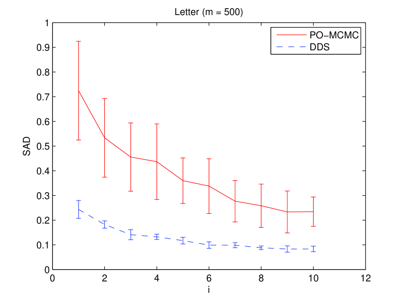
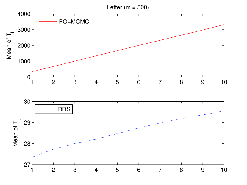
Finally, we present the experimental results for the DDS by varying the sample size. We first choose the data case Letter with $m=500$ as an example. For the DDS, we tried sample size $N_{o}$ $=5,000\cdot i$, where $i\in\{1,2,\ldots,10\}$. For each $i$, we independently ran the DDS $15$ times to get the sample mean and the sample standard deviation of SAD for the (directed) edge features. For the PO-MCMC, with the bucket size $b=10$, we ran totally $5,000\cdot i$ MCMC iterations in the partial order space, where $i\in\{1,2,\ldots,10\}$. For each $i$, we discarded the first $2,500\cdot i$ MCMC iterations for “burn-in” and set the thinning parameter to be $50$ so that $50\cdot i$ partial orders finally got sampled. Again, for each $i$, we independently ran the PO-MCMC $15$ times to get the sample mean and the sample standard deviation of SAD for the edge features.

Figure 2 shows the SAD performance of the two methods with each $i$ in terms of the edge features, where an error bar represents one sample standard deviation $\hat{\sigma}$(SAD) across $15$ runs from a method (the PO-MCMC or the DDS) at each $i$. For example, Figure 2 shows that when $i=4$, $\hat{\mu}$(SAD) $=0.1326$ and $\hat{\sigma}$(SAD) $=0.0107$ from our DDS algorithm; while $\hat{\mu}$(SAD) $=0.4369$ and $\hat{\sigma}$(SAD) $=0.1529$ from the PO-MCMC method. This exactly matches the results previously shown in Table 1. Correspondingly, Figure 2 shows $\hat{\mu}(T_{t})$ (the sample mean of the total running time) of the PO-MCMC and the DDS with each $i$, where the running time is in seconds. The advantage of our DDS can be clearly seen by combining Figures 2 and 2. For each $i\in\{1,2,\ldots,10\}$, the real mean of SAD from the DDS is significantly smaller than the one from the PO-MCMC with the p-value $<5\times 10^{-3}$ returned by the two-sample $t$ test (with unequal variances). In terms of the running time, the total running time of the DDS is very short relative to the one of the PO-MCMC. For example, $\hat{\mu}(T_{t})$ of the DDS increases with respect to $i$ and reaches only $29.55$ seconds at $i=10$. This is shorter than $9\%$ of $\hat{\mu}(T_{t})$ of the PO-MCMC at $i=1$, which is $336.09$ seconds. Therefore, the learning performance of the DDS with each sample size is significantly better than the one of the PO-MCMC for the data case Letter with $m=500$.

We also performed the experiment with the same experimental settings for the data cases Tic-Tac-Toe, Wine, Child with $m=500$, and German. Please refer to the supplementary material for the experimental results. (The supplementary material is available at http://www.cs.iastate.edu/~jtian/Software/BNLearner/BN_Learning_Sampling_Supplement.pdf. ) The same conclusion about the learning performance can be clearly drawn by examining the figures shown in the supplementary material.

Figure 1: Plot of the SAD Performance of the PO-MCMC and the DDS for Letter ($m=500$)

Figure 2: Plot of the Total Running Time of the PO-MCMC and the DDS for Letter ($m=500$)

4.2 Experimental Results for the IW-DDS

In this subsection, we compare our IW-DDS algorithm with the Hybrid MCMC (i.e., DP+MCMC) method (Eaton and Murphy, 2007) and the $K$-best algorithm (Tian et al., 2010), two state-of-the-art methods that can estimate the posteriors of any features without the order-modular prior assumption. The implementation of the Hybrid MCMC (called BDAGL) and the implementation of the $K$-best (called KBest) are both made available online by their corresponding authors. (BDAGL is available at http://www.cs.ubc.ca/~murphyk/Software/BDAGL/.) (KBest is available at http://www.cs.iastate.edu/~jtian/Software/UAI-10/KBest.htm.)

Since $n$ in each investigated data case is moderate, we are able to use POSTER, a C++ language implementation of the DP algorithm of Tian and He (2009) to get $p_{\nprec}(i\rightarrow j|D)$, the exact posterior of each edge $i\rightarrow j$ under the structure-modular prior. (POSTER is available at http://www.cs.iastate.edu/~jtian/Software/UAI-09/Poster.htm.) Therefore we can use the SAD criterion ($\sum_{ij}|p_{\nprec}(i\rightarrow j|D)$ $-\hat{p}_{\nprec}(i\rightarrow j|D)|$) to measure the performance of these three methods in the structural learning for each data case.

For fair comparison, in our algorithm we used the BDeu score (Heckerman et al., 1995) with equivalent sample size 1 and set $p_{i}(Pa_{i})(\equiv\rho_{i}(Pa_{i}))\equiv 1$, since these settings are also used in POSTER and the implementation of the $K$-best algorithm.

Name	$n$	$m$	DP	DP+MCMC		$K$-best	IW-DDS		$K$-best	IW-DDS
			SAD	$\hat{\mu}$(SAD)	$\hat{\sigma}$(SAD)	SAD	$\hat{\mu}$(SAD)	$\hat{\sigma}$(SAD)	$\Delta$	$\hat{\mu}$($\Delta$)	$\hat{\sigma}$($\Delta$)
T-T-T	10	958	0.1651	15.0079	2.9877	1.4194	0.0227	0.0102	6.943E-01	9.935E-01	8.636E-04
Glass	11	214	1.5444	0.3587	0.4599	0.0904	0.0381	0.0019	9.780E-01	9.901E-01	6.368E-04
Wine	13	178	1.4786	0.4605	0.2968	0.2011	0.1041	0.0075	9.023E-01	9.670E-01	1.700E-03
Housing	14	506	5.6478	8.0000	3.3408	9.1179	4.8276	0.0624	2.880E-02	1.096E-01	1.200E-03
Credit	16	690	4.0580	5.0261	2.3482	5.1492	2.9148	0.0336	5.010E-02	1.793E-01	1.700E-03
Zoo	17	101	8.2142	32.4189	10.0953	35.1215	19.7025	4.0767	3.815E-08	1.652E-11	1.211E-11
Tumor	18	339	5.1536	17.5104	7.9198	20.5793	10.3139	0.6950	2.940E-05	3.619E-06	3.586E-07
Vehicle	19	846	3.5759	3.8234	0.4011	3.3683	0.4648	0.0194	5.387E-01	9.432E-01	2.600E-03
German	21	1,000	3.7261	5.0207	3.2223	5.5902	0.9891	0.0449	7.800E-02	7.422E-01	7.200E-03
Syn15	15	100	4.9321	12.8705	7.6384	11.8685	10.1341	0.1495	1.604E-04	1.183E-04	4.664E-06
		200	3.2557	4.5090	2.5875	7.5232	4.9079	0.0583	2.700E-03	7.300E-03	1.265E-04
		500	6.9798	5.5466	1.9175	4.4379	4.2965	0.1619	1.526E-01	2.388E-01	4.900E-03
		1,000	1.3000	0.3974	0.3299	0.0848	0.0498	0.0048	9.699E-01	9.843E-01	8.909E-04
		2,000	1.7192	1.8263	1.7095	0.3701	0.1081	0.0147	8.521E-01	9.703E-01	3.300E-03
		5,000	1.9473	0.0304	0.0094	8.89E-04	0.0022	0.0002	9.998E-01	9.994E-01	9.821E-05
Letter	17	100	9.2140	27.1507	4.0940	24.4313	15.8780	0.2764	2.908E-04	1.621E-04	5.336E-06
		200	7.2855	15.1587	3.5615	9.4512	6.7936	0.1191	7.800E-03	1.220E-02	3.341E-04
		500	6.0961	3.4637	4.6789	1.7237	0.6347	0.0119	6.948E-01	8.808E-01	3.000E-03
		1,000	0.6394	0.1761	0.0166	0.0837	0.0766	0.0039	9.834E-01	9.864E-01	8.678E-04
		2,000	2.3913	3.5085	3.1132	2.0976	0.1338	0.0213	6.859E-01	9.756E-01	2.700E-03
		5,000	0.8407	0.1182	0.0442	0.0160	0.0072	0.0005	9.948E-01	9.972E-01	2.077E-04
Insur19	19	100	5.3356	9.4318	3.9576	11.7779	6.5062	0.0891	6.000E-03	2.010E-02	4.767E-04
		200	5.9844	5.5465	2.7295	2.2572	1.4630	0.0557	4.495E-01	7.049E-01	1.120E-02
		500	1.8274	0.3605	0.2287	0.4970	0.1328	0.0105	7.464E-01	9.379E-01	3.000E-03
		1,000	1.7386	0.2186	0.0762	0.7498	0.0623	0.0111	5.866E-01	9.785E-01	2.600E-03
		2,000	1.2737	0.1217	0.0380	0.0174	0.0062	0.0012	9.900E-01	9.976E-01	4.864E-04
		5,000	1.9511	0.1765	0.0594	0.0103	0.0092	0.0010	9.970E-01	9.973E-01	2.086E-04
Child	20	100	6.9783	11.8987	3.1086	11.6189	7.0304	0.0909	7.848E-04	2.700E-03	1.066E-04
		200	3.2826	4.7066	4.3749	5.0729	2.8510	0.0192	4.800E-03	1.506E-01	1.200E-03
		500	2.5580	2.4716	1.3489	1.5304	0.5416	0.0305	3.582E-01	8.222E-01	5.100E-03
		1,000	2.4708	2.6061	2.2909	0.7066	0.1499	0.0198	7.013E-01	9.545E-01	3.400E-03
		2,000	2.3330	1.4286	1.2290	1.5279	0.0662	0.0161	6.509E-01	9.828E-01	2.800E-03
		5,000	2.0365	1.2533	1.7313	0.8783	0.0150	0.0013	8.209E-01	9.940E-01	4.696E-04

Table 3: Comparison of the DP+MCMC, the $K$-best & the IW-DDS in Terms of SAD

Name	$n$	$m$	DP+MCMC	$K$-best	IW-DDS	IW-DDS
			$\hat{\mu}(T_{t})$	$T_{t}$	$\hat{\mu}(T_{t})$	$\hat{\mu}(T_{DP})$	$\hat{\sigma}(T_{DP})$	$\hat{\mu}(T_{ord})$	$\hat{\sigma}(T_{ord})$	$\hat{\mu}(T_{DAG})$	$\hat{\sigma}(T_{DAG})$
T-T-T	10	958	1.29 + 1,032.40	8.37	3.28	1.27	0.0060	1.57	0.0109	0.44	0.0128
Glass	11	214	1.04 + 1,037.26	18.13	1.72	0.98	0.0210	0.50	0.0054	0.24	0.0018
Wine	13	178	2.44 + 1,127.80	141.20	3.52	2.15	0.0199	0.63	0.0061	0.74	0.0057
Housing	14	506	4.83 + 1,421.00	323.37	5.67	4.21	0.0813	0.63	0.0042	0.52	0.0043
Credit	16	690	33.73 + 1,476.90	2,073.41	35.20	29.30	0.3322	0.81	0.0055	4.94	1.6191
Zoo	17	101	22.33 + 2,107.50	5,531.81	26.16	12.49	0.1853	1.11	0.0048	12.05	0.1898
Tumor	18	339	60.86 + 1,799.99	18,640.09	87.35	39.49	0.4419	1.19	0.0184	46.31	0.2937
Vehicle	19	846	207.27 + 1,886.10	17,126.45	171.75	160.55	0.9310	1.49	0.0175	9.67	0.0665
German	21	1,000	600.19 + 1,849.90	10,981.29	540.61	392.25	2.8656	1.68	0.0207	146.65	1.4290
Syn15	15	100	5.21 + 1,284.00	889.97	9.41	3.56	0.0667	0.81	0.0048	4.80	0.0273
		200	6.28 + 1,286.20	901.23	10.29	4.76	0.2090	0.80	0.0111	4.53	0.0256
		500	9.64 + 1,336.80	899.42	9.59	7.50	0.0821	0.85	0.0051	1.08	0.0128
		1,000	13.69 + 1,364.60	910.76	13.35	12.15	0.7578	0.85	0.0156	0.33	0.0038
		2,000	22.64 + 1,372.10	907.02	21.98	20.81	0.5200	0.85	0.0061	0.30	0.0019
		5,000	54.79 + 1,356.70	932.96	52.07	47.80	1.0887	3.99	0.0235	0.28	0.0023
Letter	17	100	25.53 + 1,572.60	7,639.02	20.27	15.83	0.0601	1.15	0.0062	2.83	0.0292
		200	30.01 + 1,576.80	7,966.25	25.87	20.22	0.1769	1.09	0.0069	4.21	0.0304
		500	39.58 + 1,598.90	8,257.60	31.88	29.84	0.1575	0.95	0.0055	1.01	0.0123
		1,000	52.85 + 1,575.60	8,380.57	44.48	42.93	0.4835	0.98	0.0093	0.56	0.0100
		2,000	77.48 + 1,591.00	7,619.29	69.14	66.34	0.5184	2.01	0.0241	0.78	0.0068
		5,000	157.69 + 1,636.40	8,134.85	136.95	134.94	1.6127	1.36	0.0097	0.65	0.0067
Insur19	19	100	101.47 + 1,828.00	6,745.41	112.28	55.85	0.1540	1.41	0.0117	54.71	0.5438
		200	113.79 + 1,896.10	6,783.76	82.52	68.12	0.4187	1.45	0.0120	12.90	0.1329
		500	137.18 + 1,864.40	6,894.15	98.96	91.44	0.4547	1.43	0.0128	6.07	0.0358
		1,000	168.55 + 1,862.30	6,966.90	133.87	123.42	0.8007	1.44	0.0157	9.00	0.0601
		2,000	226.36 + 1,781.70	7,277.60	185.02	177.66	1.3165	3.30	0.0483	4.06	0.0356
		5,000	380.78 + 1,814.80	7,061.76	336.03	329.78	4.5841	1.89	0.0220	4.34	0.0713
Child	20	100	203.44 + 1,785.10	15,085.86	223.62	106.01	0.3976	1.67	0.0176	115.60	1.3183
		200	215.70 + 1,760.80	14,222.86	225.76	119.82	1.8604	1.69	0.0107	104.09	0.9659
		500	248.17 + 1,818.70	14,016.94	214.91	149.73	0.8344	1.67	0.0183	63.48	0.5783
		1,000	292.40 + 1,817.20	15,504.82	232.11	193.18	1.1041	1.72	0.0135	37.20	0.3176
		2,000	371.12 + 1,841.40	16,109.91	306.42	268.78	2.3209	1.82	0.0165	35.81	0.3680
		5,000	589.99 + 1,846.40	15,372.61	524.63	483.90	6.7403	1.93	0.0160	38.80	0.5411

Table 4: Comparison of the DP+MCMC, the $K$-best & the IW-DDS in Terms of Time (Time Is in Seconds)

As for the DP+MCMC, we note that most part of its implementation in BDAGL tool is written in Matlab, whereas both the K-best and the IW-DDS are implemented in C++. In order to make relatively fair comparison in terms of the running time, we used REBEL tool, a C++ implementation of the DP algorithm of Koivisto (2006), to perform the computation in the DP phase of the DP+MCMC; but for fair comparison we changed its scoring criterion into the BDeu score with equivalent sample size 1 and set $q_{i}(U_{i})\equiv 1$ and $\rho_{i}(Pa_{i})\equiv 1$. To perform the computation in the MCMC phase, we used the Matlab implementation of BDAGL and we ran it under Windows 7 on an ordinary laptop with 2.40 Intel Core i5 CPU and 4.0 GB memory. The MCMC used the pure global proposal (with local proposal choice $\beta$ = 0) since such a setting was reported by Eaton and Murphy (2007) to have the best performance for edge discovery when up to about $190,000$ MCMC iterations were performed in their experimental results. We ran totally 190,000 MCMC iterations each time and discarded the first 100,000 iterations as the burn-in period. Then we set the thinning parameter to be 3 to get the final 30,000 DAG samples. As a result, the time statistics of the DP phase (the number before + sign in Table 4) but not the MCMC phase (the number after + sign) can be directly compared with the ones of the other two methods. For each data case, we performed 20 independent MCMC runs based on the DP outcome from REBEL to get the results.

For our IW-DDS, we set $N_{o}=30,000$. We performed 20 independent runs for each data case to get the results. For the $K$-best, note that its SAD is fixed since there is no randomness in the computed results. So we only ran it once to get the result. We set $K$ to be $100$ for Tic-Tac-Toe, Glass, Wine, Housing, Credit, Zoo, Syn15, and Letter, that is, we got the $100$ best DAGs from Tic-Tac-Toe, Glass, Wine, Housing, Credit, Zoo, each of the six cases of Syn15, and each of the six cases of Letter. We set $K$ to be only $80$ for Tumor because our experiments showed that for Tumor the $K$-best program ran out of memory with $K>80$. Due to the same out-of-memory issue, we set $K$ to be only $40$ for Vehicle and Insur19; and we set $K$ to be only $20$ for Child and $9$ for German. The fact that $K$ can only take a value no greater than $40$ for $n$ $\geq 19$ in our experiments confirms our claim about the computation problem of the $K$-best algorithm in terms of its space cost.

Table 3 shows the experimental results in terms of SAD for each data case while Table 4 shows the running time costs corresponding to Table 3. (Just as Table 2, Table 4 also lists the sample mean and the sample standard deviation of the running time of three steps of the DDS in the IW-DDS algorithm.) The column named DP in Table 3 shows the SAD ($\sum_{ij}|p_{\nprec}(i\rightarrow j|D)$ $-p_{\prec}(i\rightarrow j|D)|$), where each edge posterior $p_{\nprec}(i\rightarrow j|D)$ is computed by the exact DP method of Tian and He (2009), and each edge posterior $p_{\prec}(i\rightarrow j|D)$ is computed by the exact DP method of Koivisto (2006). The SAD values reported in this column indicate the bias due to the assumption of the order-modular prior. Next to the DP column, the SAD values of the three methods are listed in Table 3. Both the DP+MCMC method and the IW-DDS method are random so that both $\hat{\mu}$(SAD) and $\hat{\sigma}$(SAD) are shown for these two methods. The outcome of the $K$-best algorithm is not random so that only its SAD is shown. Finally Table 3 also shows the cumulative posterior probability mass $\Delta$ for both the $K$-best algorithm and the IW-DDS method.

Tables 3 and 4 clearly demonstrate the advantage of our method over the other two methods. By using much shorter computation time, our method has its $\hat{\mu}$(SAD) less than the corresponding one from the DP+MCMC for 32 out of the 33 data cases. The only exceptional case is Syn15 with $m=200$. Furthermore, based on the two-sample $t$ test with unequal variances, we can conclude at the significance level 0.05 that the real mean of SAD using our method is less than the corresponding one using the DP+MCMC for each of the 31 cases; the two exceptional cases are Syn15 with $m=100$ and Syn15 with $m=200$. (For 30 out of these 31 cases, the p-value of the two-sample $t$ test is less than $0.01$.) Meanwhile, $\hat{\sigma}$(SAD) using our method is always much smaller than the one using the DP+MCMC for each of the 33 cases, which indicates higher stability of the performance of our method. Similarly, using much shorter computation time, our method has its $\hat{\mu}$(SAD) less than the SAD from the $K$-best for 32 out of the 33 cases. The only exception is Syn15 with $m$ = 5,000. Furthermore, based on the one-sample $t$ test (Casella and Berger, 2002), we can conclude at the significance level $5\times 10^{-4}$ that the real mean of SAD using our method is less than the SAD using the $K$-best for each of these 32 cases.

There are several other interesting things shown in Tables 3 and 4. In terms of the SAD, for very small $m$, $\hat{\mu}$(SAD) using the DP+MCMC method is even larger than the SAD from the DP phase (Koivisto, 2006) itself. For example, for the data case Zoo, the SAD from the DP phase is $8.2142$ but $\hat{\mu}$(SAD) obtained after the MCMC phase of the DP+MCMC method is $32.4189$. Similar situations also occur in Syn15, Letter, Insur19, and Child when $m=100$. This indicates that for very small $m$, the MCMC phase of the DP+MCMC method is unable to reduce the bias from the DP method of Koivisto (2006) for all these cases based on $190,000$ MCMC iterations. As for the running time, please note that $\hat{\mu}$($T_{DP}$) of our IW-DDS is always less than the running time of the DP phase of the DP+MCMC method. This is because the DP step of our method uses the DP algorithm of Koivisto and Sood (2004), that is, the first three steps of the DP algorithm of Koivisto (2006); while the DP phase of the DP+MCMC method uses all the five steps of the DP algorithm of Koivisto (2006). In other words, compared with the DP algorithm of Koivisto and Sood (2004), the DP algorithm of Koivisto (2006) includes a larger constant factor hidden in the $O(n^{k+1}C(m)+kn2^{n})$ notation though these two DP algorithms have the same time complexity. This difference will make the total running time of our IW-DDS even less than the running time of the DP phase of the DP+MCMC method when the remaining steps of the IW-DDS run faster than the last two steps of the DP algorithm of Koivisto (2006). For example, for the data case Child with $m=5,000$, $\hat{\mu}(T_{t})$ of the IW-DDS is $524.63$ seconds while the corresponding running time of the DP phase of the DP+MCMC method is $589.99$ seconds. Actually, Table 4 shows that there are 21 out of the 33 cases where $\hat{\mu}(T_{t})$ of the IW-DDS is less than the running time of the DP phase of the DP+MCMC method. In addition, just as shown in Section 4.1, the effectiveness of our time-saving strategy can also be clearly seen from Table 4. For example, the ratio of $\hat{\mu}(T_{DAG})$ to $\hat{\mu}(T_{ord})$ ranges from 0.07 to 87.29 across the 33 cases, which is much smaller than the upper bound of the ratio of $O(n^{k+1}N_{o})$ to $O(n^{2}N_{o})$.

Table 3 also shows the resulting cumulative probability mass $\Delta$ from the $K$-best and our IW-DDS for all the data cases. (Note that $\Delta$ is computed by the formula $\Delta$ $=\sum_{G\in\mathcal{G}}p_{\nprec}(G,D)/p_{\nprec}(D)$, where $p_{\nprec}(D)$ is computed using POSTER tool.) In the table, $\hat{\mu}$($\Delta$) from our IW-DDS is greater than $\Delta$ from the $K$-best for 28 out of the 33 data cases. The five exceptional cases are Zoo, Tumor, Syn15 with $m=100$, Syn15 with $m=5,000$, and Letter with $m=100$. Interestingly, for four out of the five exceptional cases (as well as the other 28 cases), $\hat{\mu}$(SAD) from our IW-DDS is significantly smaller than SAD from the $K$-best. One possible reason is that the $K$ best DAGs tend to have the same or similar local structures (family $(i,Pa_{i})$’s) that have relatively large local scores while a large number of DAGs sampled from our IW-DDS include various local structures for each node $i$. When $\Delta$ is far below $1$, the inclusion of various local structures seems to be more effective in improving the structural learning performance.

In addition, Table 3 shows that when $m$ is not very small (such as no smaller than $1,000$), $\Delta$ from our IW-DDS with $N_{o}=30,000$ can reach a large percentage (such as greater than $90\%$) in most of our data cases. As a result, we can obtain a sound interval for $p_{\nprec}(f|D)$ with a small width (such as less than $0.1$) for any feature $f$.

To further demonstrate that our IW-DDS can obtain a large $\Delta$ efficiently when $m$ is not very small, we increased $N_{o}$ from $100,000$ to $600,000$ with each increment $100,000$ to see its performance for the data cases Letter with $m=500$, Child with $m=500$, and German. Again, we performed 20 independent runs for each data case to get the results. Figures 8, 8 and 8 show the increase in $\Delta$ with respect to the increase in $N_{o}$ for these three data cases. Correspondingly, Figures 8, 8 and 8 indicate the increase in $\hat{\mu}(T_{t})$, $\hat{\mu}(T_{ord})$ and $\hat{\mu}(T_{DAG})$ with respect to the increase in $N_{o}$ for these three data cases, where the running time is in seconds. Combining these figures, it is clear that our IW-DDS can efficiently achieve a large $\Delta$. Take the data case German for example, with the time cost $\hat{\mu}(T_{t})$ = $1,493.02$ seconds, our IW-DDS can collect $N_{o}=600,000$ DAG samples so that the corresponding mean of $\Delta$ can reach $91.74\%$. Therefore, for any feature $f$ in the data case German, our IW-DDS can provide a sound interval for $p_{\nprec}(f|D)$ with width $0.0826$. Note that the $K$-best can only provide a meaningless sound interval for $p_{\nprec}(f|D)$ with huge width $0.922$ because its $\Delta$ can only reach $0.078$ in the data case German before running out of the memory. Also note that the ratio of $\hat{\mu}(T_{DAG})$ to $\hat{\mu}(T_{ord})$ decreases from $56.45$ to $30.95$ when $N_{o}$ increases from $100,000$ to $600,000$. (The increase rate of $\hat{\mu}(T_{ord})$ is a constant with respect to $N_{o}$; but the increase rate of $\hat{\mu}(T_{DAG})$ actually decreases as $N_{o}$ increases.) This witnesses the statement in Remark 5 that the benefit from our time-saving strategy will typically increase when $N_{o}$ increases.

Figure 3: Plot of $\Delta$ versus $N_{o}$ for Letter ($m=500$)

Figure 4: Plot of the Running Time versus $N_{o}$ for Letter ($m=500$)

Figure 5: Plot of $\Delta$ versus $N_{o}$ for Child ($m=500$)

Figure 6: Plot of the Running Time versus $N_{o}$ for Child ($m=500$)

Figure 7: Plot of $\Delta$ versus $N_{o}$ for German

Figure 8: Plot of the Running Time versus $N_{o}$ for German

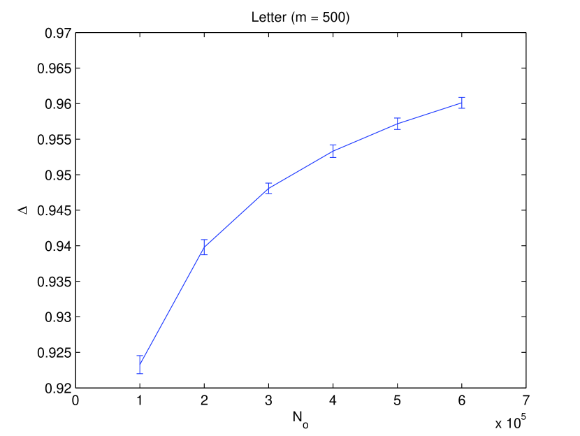
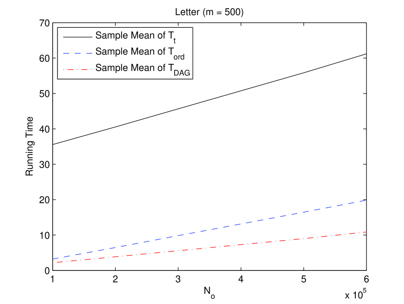
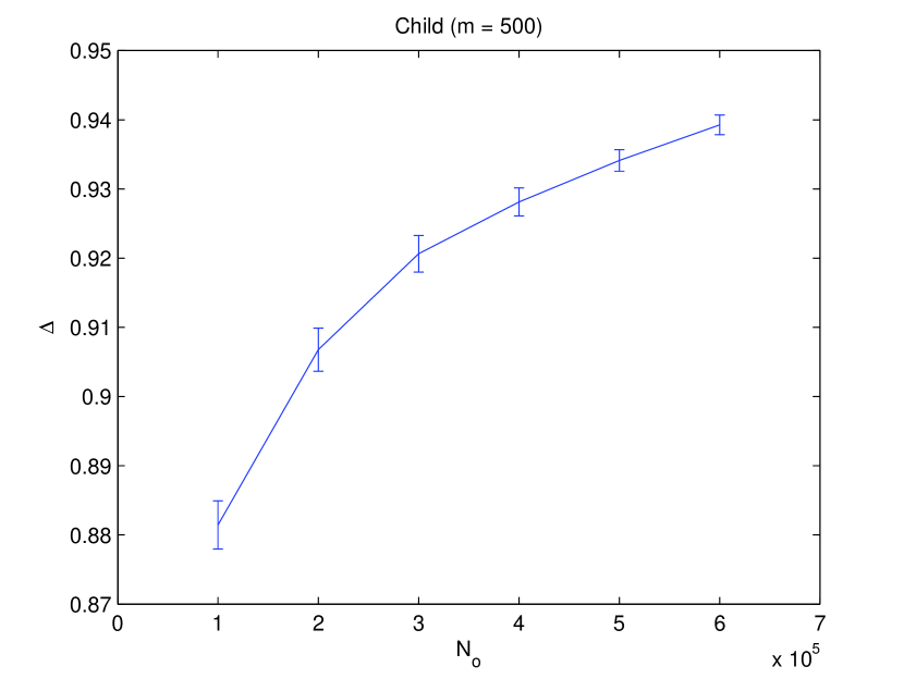
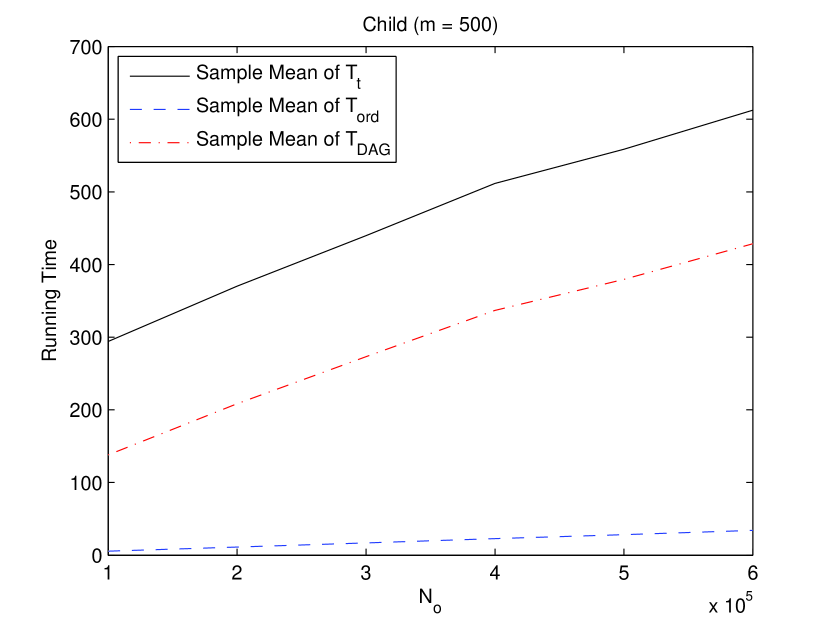
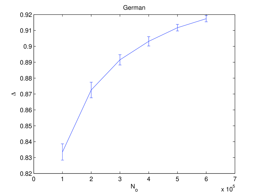
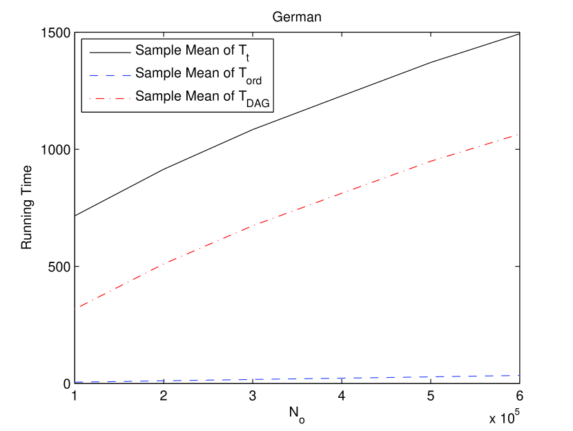
Finally, we present the experimental results for the IW-DDS by varying the sample size. Just as Section 4.1, the experiments were performed for the five data cases Tic-Tac-Toe, Wine, Letter with $m=500$, Child with $m=500$, and German. For the IW-DDS, we tried the sample size $N_{o}$ $=5,000\cdot i$, where $i\in\{1,2,\ldots,10\}$. For each $i$, we independently ran the IW-DDS $20$ times to get the sample mean and the sample standard deviation of SAD for the (directed) edge features. For the DP+MCMC, we ran totally $50,000\cdot i$ MCMC iterations, where $i\in\{1,2,\ldots,10\}$. For each $i$, we discarded the first $25,000\cdot i$ MCMC iterations for “burn-in” and set the thinning parameter to be $5$ so that $5,000\cdot i$ DAGs got sampled. Again, for each $i$, we independently ran the MCMC $20$ times to get the sample mean and the sample standard deviation of SAD for the edge features. As for the $K$-best, different experimental settings were used for different data cases due to the out-of-memory issue. For two data cases Tic-Tac-Toe and Wine, we ran the $K$-best program with $K=20\cdot i$, where $i\in\{1,2,\ldots,10\}$. (The setting of $K=20\cdot i$ guarantees that for these two data cases the running time of the $K$-best is longer than the running time of the IW-DDS at each $i$, which will be demonstrated soon.) For the data case Letter with $m=500$, we only ran the $K$-best with $K=162$ because the $K$-best program will run out of memory when $K>162$ due to its expensive space cost. The corresponding result of the $K$-best would be compared with the result of the IW-DDS at $i=10$ (i.e., the IW-DDS with $N_{o}=50,000$). For the same out-of-memory issue, we only set $K=20$ for Child with $m=500$ and set $K=9$ for German when running the $K$-best program. Note that since there is no randomness in the outcome of the $K$-best algorithm, we always ran the $K$-best program only once to get its fixed SAD for the edge features.

The experimental results of comparing the three methods based on the data case Tic-Tac-Toe are shown in Figures 10 and 10. Figure 10 shows the SAD performance of the three methods with each $i$ $\in\{1,2,\ldots,10\}$ in terms of the edge features, where an error bar represents one sample standard deviation $\hat{\sigma}$(SAD) across $20$ runs from the DP+MCMC or the IW-DDS at each $i$. Figure 10 shows $\hat{\mu}(T_{t})$ (the sample mean of the total running time) of the DP+MCMC and the IW-DDS as well as $T_{t}$ (the total running time) of the $K$-best with each $i$, where the running time is in seconds. The advantage of our IW-DDS can be clearly seen by combining Figures 10 and 10. Comparing with the DP+MCMC, for each $i\in\{1,2,\ldots,10\}$, the IW-DDS uses the shorter running time but has its real mean of SAD significantly smaller than the corresponding real mean of SAD from the DP+MCMC, with the p-value $<1\times 10^{-10}$ from the two-sample $t$ test with unequal variances. Comparing with the $K$-best, for each $i\in\{1,2,\ldots,10\}$, the IW-DDS uses the shorter running time than the $K$-best, but the IW-DDS has its real mean of SAD significantly smaller than the SAD from the $K$-best, with the p-value $<1\times 10^{-35}$ from the one-sample $t$ test. Therefore, the learning performance of the IW-DDS is significantly better than the performance of the other two methods at each $i$ for the data case Tic-Tac-Toe.

The experimental results based on the data case Letter with $m=500$ are shown in Figures 12 and 12. Just as the description for Figures 10 and 10, Figure 12 shows the SAD performance of the three methods in terms of the edge features, and Figure 12 shows the corresponding time costs of the three methods. The only difference is that in both Figure 12 and Figure 12, the corresponding result of the $K$-best with $K=162$ is marked as a star and compared with the one of the IW-DDS at $i=10$. The advantage of our IW-DDS can be clearly seen by combining Figures 12 and 12. Comparing with the DP+MCMC, for each $i\in\{1,2,\ldots,10\}$, the IW-DDS uses the much shorter running time but has its real mean of SAD significantly smaller than the corresponding real mean of SAD from the DP+MCMC, with the p-value $<0.013$ from the two-sample $t$ test with unequal variances. ($\hat{\mu}(T_{t})$ of the IW-DDS at $i=10$ is only $33.00$ seconds, which is even less than the running time of the DP phase of the DP+MCMC method ($39.58$ seconds).) Note that $\hat{\sigma}$(SAD) from the DP+MCMC is shown to be very large. The DP+MCMC has its $\hat{\sigma}$(SAD) even larger than its $\hat{\mu}$(SAD) (the sample mean of SAD) when $i\geq 8$, which indicates that the performance of the DP+MCMC is not stable based on the 500,000 MCMC iterations. Comparing with the $K$-best, the IW-DDS with $N_{o}=50,000$ uses the much shorter running time but has its real mean of SAD significantly smaller than the SAD from the $K$-best with $K=162$ since the p-value from the corresponding one-sample $t$ test is less than $1\times 10^{-35}$. Therefore, the learning performance of the IW-DDS is also significantly better than the performance of the other two methods for the data case Letter with $m=500$.

The experimental results for the other three data cases Wine, Child with $m=500$, and German are represented similarly in the supplementary material. The same conclusion about the learning performance can be clearly drawn by examining the figures shown in the supplementary material.

Figure 9: Plot of the SAD Performance of the DP+MCMC, the $K$-best and the IW-DDS for Tic-Tac-Toe

Figure 10: Plot of the Total Running Time of the DP+MCMC, the $K$-best and the IW-DDS for Tic-Tac-Toe

Figure 11: Plot of the SAD Performance of the DP+MCMC, the $K$-best and the IW-DDS for Letter ($m=500$)

Figure 12: Plot of the Total Running Time of the DP+MCMC, the $K$-best and the IW-DDS for Letter ($m=500$)

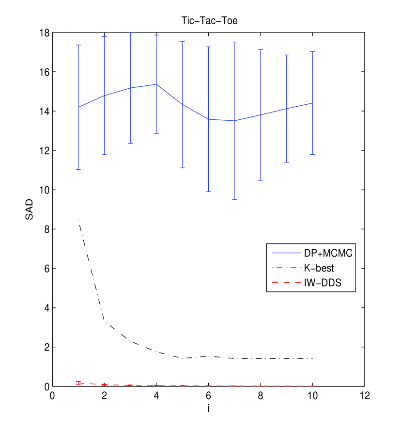
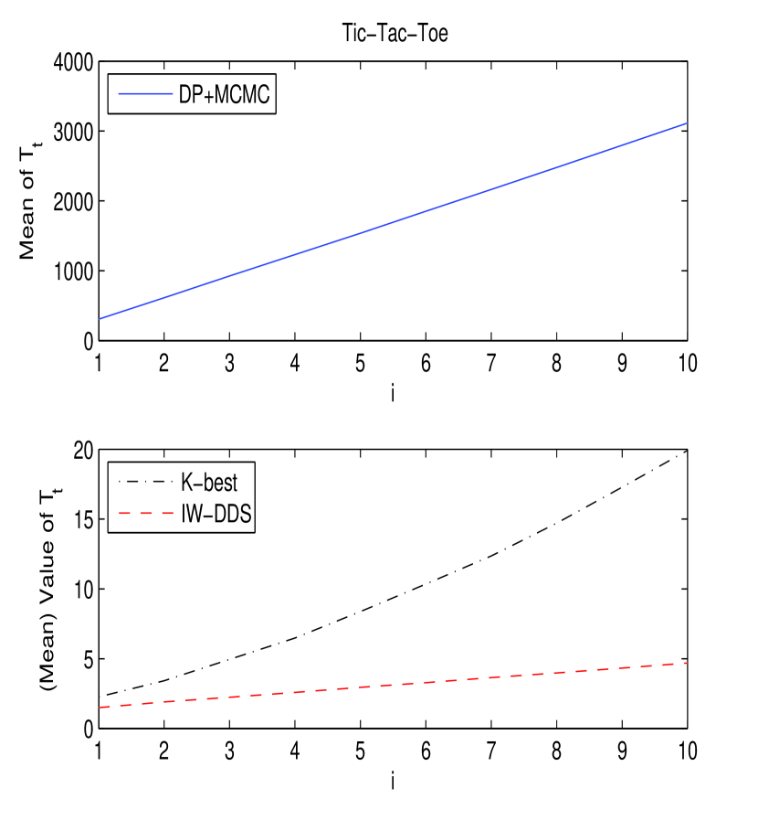
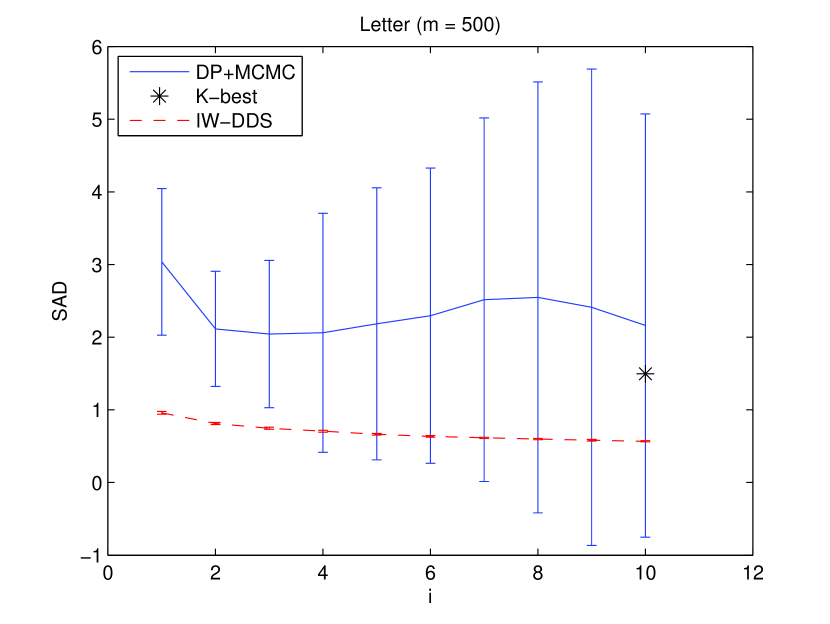
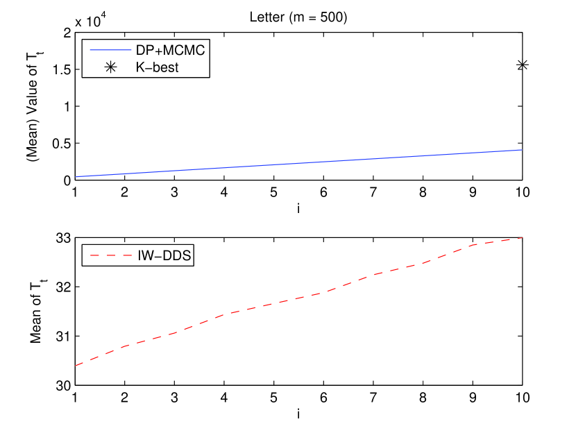
4.3 Learning Performance of Non-modular Features

In Sections 4.1 and 4.2 we did not provide experimental results on the learning performance of non-modular features. We did not do so in Section 4.2 because there is no known method to compute the true/exact posterior probability of any non-modular feature $p_{\nprec}(f|D)$ except by the brute force enumeration over all the (super-exponential number of) DAGs so that the quality of the corresponding $\hat{p}_{\nprec}(f|D)$ learned from any approximate method cannot be precisely measured. We did not do so in Section 4.1 because the current PO-MCMC tool (BEANDisco) only supports the estimation of the posterior of an edge feature so that the comparison of our method and the PO-MCMC can only be made for the edge feature. (Thus, we did not make the comparison for the path feature (which is one particular non-modular feature), though the DP algorithm of Parviainen and Koivisto (2011) can compute the exact posterior of a path feature $p_{\prec}(f|D)$.) Our idea is that by showing that our algorithms have significantly better performance in computing fundamental structural features (directed edge features), which should be due to the better quality of our DAG samples with respect to the corresponding $p_{\nprec}(G|D)$ or $p_{\prec}(G|D)$, we expect that they will also be superior in computing other complicated structural features using the same set of DAG samples.

To verify our expectation, we performed the experiments on the real data set “Iris” (with $n=5$) from the UCI Machine Learning Repository (Asuncion and Newman, 2007) and the well-studied data set “Coronary” (Coronary Heart Disease) (with $n=6$) (Edwards, 2000). Since $n$ is small, by enumerating all the DAGs, we were able to compute $p_{\nprec}(f|D)$, the true posterior probability for any interesting non-modular feature $f$. For the demonstration purpose, we investigated the following five interesting non-modular features. $f_{1}$, a directed path feature from node $x$ to node $y$, denoted by $x\sim>y$, represents the situation that variable $x$ eventually influences variable $y$. $f_{2}$, a limited-length directed path feature $x\sim>y$ that has its path length no more than $2$, represents that variable $x$ can influence variable $y$ via at most one intermediate variable. $f_{3}$, a combined path feature $x\sim>y\sim>z$, can be interpreted as the situation that variable $x$ eventually influences variable $y$ which in turn eventually influences variable $z$. $f_{4}$, a combined path feature $y<\sim x\sim>z$ with $y\neq z$, means that variable $x$ eventually influences both variable $y$ and variable $z$. $f_{5}$, a combined path feature $y<\sim x\nsim>z$ with $x\neq z$, represents that variable $x$ eventually influences variable $y$ but not variable $z$. Then we compared the SAD performance of the (directed) edge feature with the corresponding SAD performance of each feature $f_{j}$ ($j\in\{1,2,3,4,5\}$) from the DP+MCMC, the $K$-best and the IW-DDS. The experimental results on both data sets show that if the SAD of the IW-DDS is significantly smaller than the SAD of the competing method (the DP+MCMC or the $K$-best) for the edge feature, then the SAD of the IW-DDS will also be significantly smaller than the SAD of the competing method for each investigated non-modular feature $f_{j}$ using the same set of DAG samples. Thus, our expectation is supported by the experiments. The detailed experimental results are as follows.

Figure 13: SAD of the Learned Edge Features for Coronary

Figure 14: SAD of the Learned $f_{1}$ Features for Coronary

Figure 15: SAD of the Learned $f_{2}$ Features for Coronary

Figure 16: SAD of the Learned $f_{3}$ Features for Coronary

Figure 17: SAD of the Learned $f_{4}$ Features for Coronary

Figure 18: SAD of the Learned $f_{5}$ Features for Coronary

Figure 19: SAD of the Learned Edge Features for Iris

Figure 20: SAD of the Learned $f_{1}$ Features for Iris

Figure 21: SAD of the Learned $f_{2}$ Features for Iris

Figure 22: SAD of the Learned $f_{3}$ Features for Iris

Figure 23: SAD of the Learned $f_{4}$ Features for Iris

Figure 24: SAD of the Learned $f_{5}$ Features for Iris

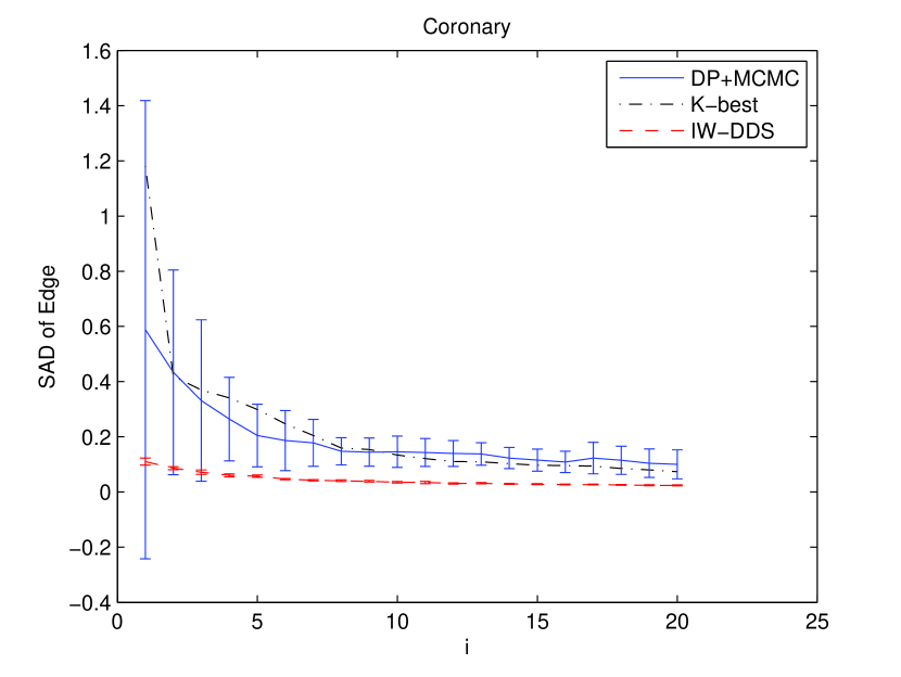
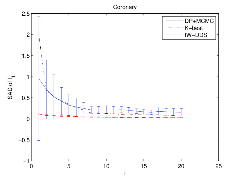
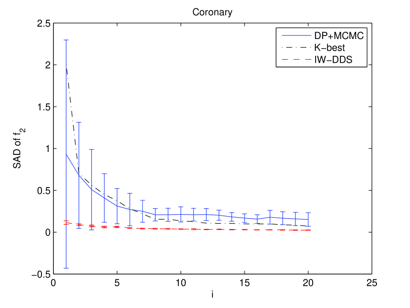
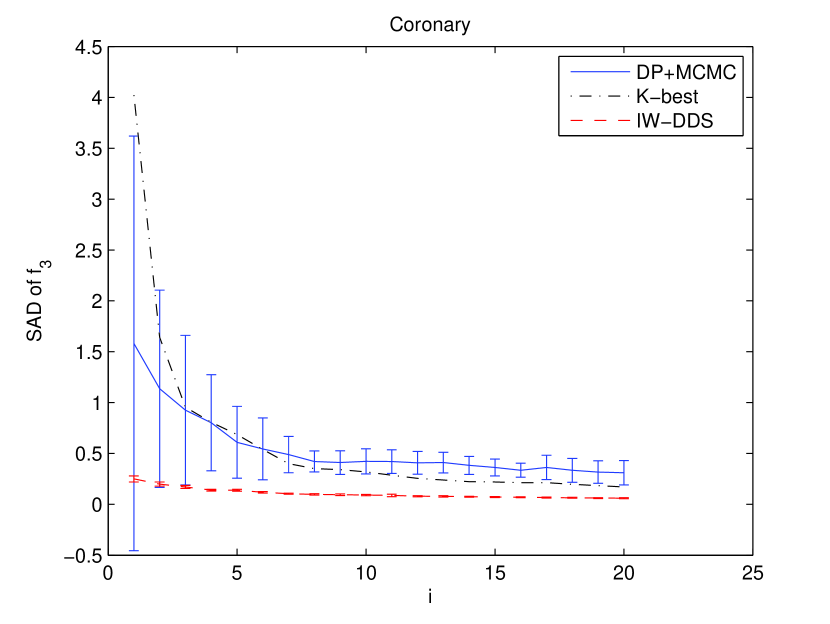
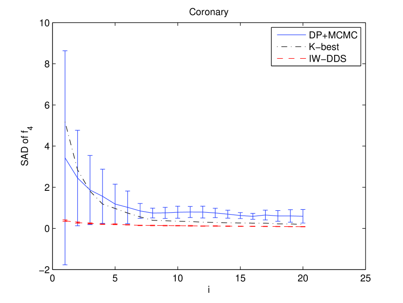
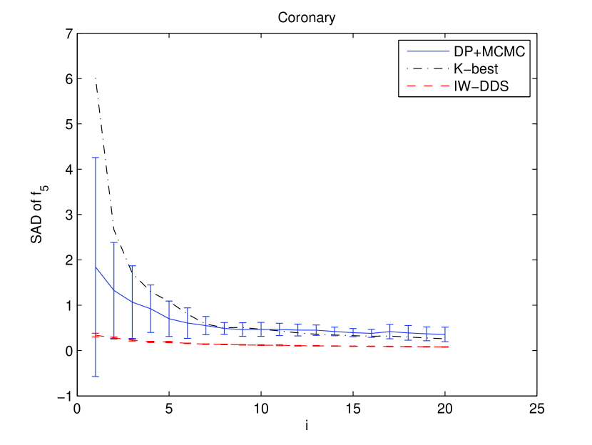
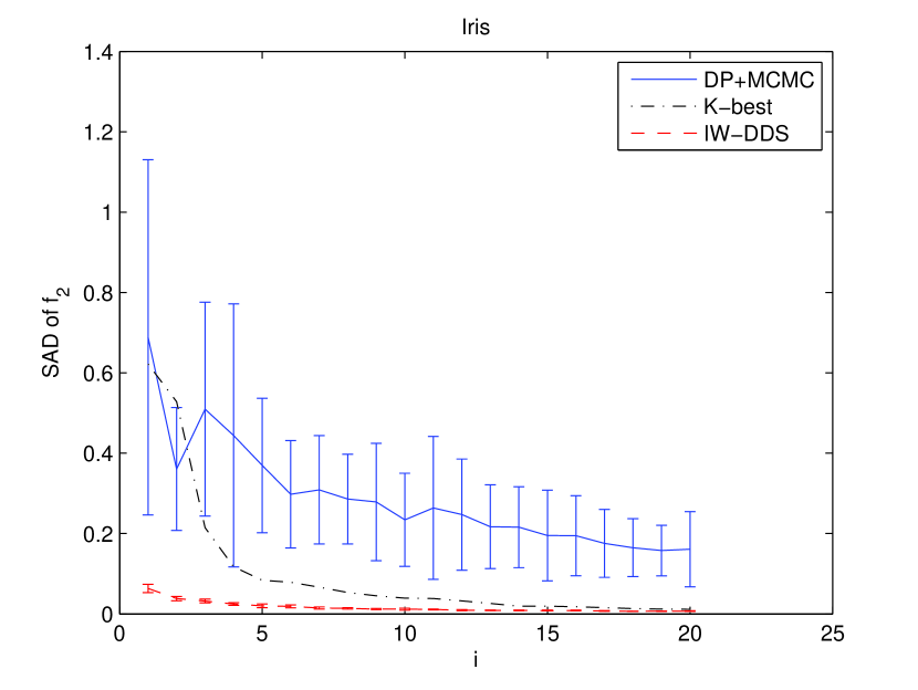
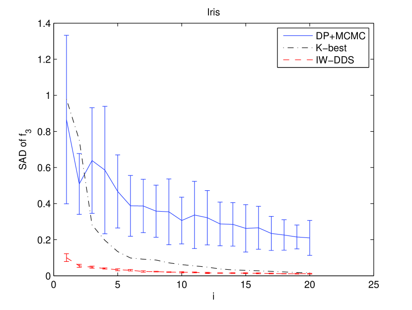
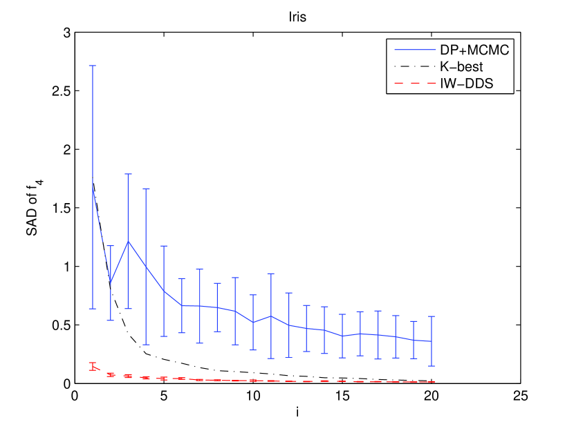
The following is our experimental design for the data set Coronary with $n=6$ and $m=1841$. For the IW-DDS, we tried the sample size $N_{o}$ $=2,500\cdot i$, where $i\in\{1,2,\ldots,20\}$. For each $i$, we independently ran the IW-DDS $20$ times to get the sample mean and the sample standard deviation of SAD for the (directed) edge feature and the five non-modular features ($f_{1}$, $f_{2}$, $f_{3}$, $f_{4}$ and $f_{5}$). For the DP+MCMC, we ran $25,000\cdot i$ MCMC iterations, where $i\in\{1,2,\ldots,20\}$. For each $i$, we discarded the first $12,500\cdot i$ MCMC iterations for “burn-in” and set the thinning parameter to be $5$ so that $2,500\cdot i$ DAGs got sampled. For each $i$, we independently ran the MCMC $20$ times to get the sample mean and the sample standard deviation of SAD for the edge feature, $f_{1}$, $f_{2}$, $f_{3}$, $f_{4}$ and $f_{5}$. For the $K$-best, we ran the $K$-best with $K=10\cdot i$, where $i\in\{1,2,\ldots,20\}$. For each $i$, we ran the $K$-best just once to get SAD for the edge feature, $f_{1}$, $f_{2}$, $f_{3}$, $f_{4}$ and $f_{5}$ since there is no randomness in the outcome of the $K$-best algorithm.

The experimental results for the data set Coronary are demonstrated from Figure 18 to Figure 18. Figure 18 shows the SAD performance of the three methods with each $i$ for the edge feature, where an error bar represents one sample standard deviation across $20$ runs for the DP+MCMC or the IW-DDS at each $i$. Correspondingly, Figure 18 to Figure 18 show the SAD performance of the three methods with each $i$ for the five investigated non-modular features ($f_{1}$, $f_{2}$, $f_{3}$, $f_{4}$ and $f_{5}$) respectively. Combining Figure 18 and each of Figures 18, 18, 18, 18, and 18, one can clearly see that if the SAD of the IW-DDS is significantly smaller than the SAD of the competing method (the DP+MCMC or the $K$-best) for the edge feature, then the SAD of the IW-DDS will also be significantly smaller than the SAD of the competing method for each of the five investigated non-modular features. More specifically, comparing with the DP+MCMC, at each $i\in\{1,2,\ldots 20\}$, for the edge feature, the real mean of SAD from the IW-DDS is significantly smaller than the corresponding one from the DP+MCMC with the p-value $<0.01$ from the two-sample $t$ test with unequal variances. Consistently, at each $i\in\{1,2,\ldots 20\}$, for each investigated non-modular feature $f_{j}$, the real mean of SAD from the IW-DDS is also significantly smaller than the corresponding one from the DP+MCMC with the p-value $<0.01$ from the same $t$ test. Comparing with the $K$-best, at each $i\in\{1,2,\ldots 20\}$, for the edge feature, the real mean of SAD from the IW-DDS is significantly smaller than the SAD from the $K$-best with the p-value $<1\times 10^{-20}$ from the one-sample $t$ test. Consistently, at each $i\in\{1,2,\ldots 20\}$, for each investigated non-modular feature $f_{j}$, the real mean of SAD from the IW-DDS is also significantly smaller than the SAD from the $K$-best with the p-value $<1\times 10^{-20}$ from the same $t$ test.

We also performed the same kind of experiments for the data set Iris with $n=5$ and $m=150$. The results are demonstrated from Figure 24 to Figure 24. Comparing with the DP+MCMC, at each $i\in\{1,2,\ldots 20\}$, just as the comparison result for the edge feature, for each investigated $f_{j}$, the real mean of SAD from the IW-DDS is also significantly smaller than the corresponding one from the DP+MCMC with the p-value $<1\times 10^{-5}$ from the two-sample $t$ test with unequal variances. Comparing with the $K$-best, at each $i\in\{1,2,\ldots 20\}$, just as the comparison result for the edge feature, for each investigated $f_{j}$, the real mean of SAD from the IW-DDS is also significantly smaller than the SAD from the $K$-best with the p-value $<1\times 10^{-9}$ from the one-sample $t$ test. Thus, a conclusion similar to the one from Coronary can be drawn: if the SAD of the IW-DDS is significantly smaller than the SAD of the competing method for the edge feature, then the SAD of the IW-DDS will also be significantly smaller than the SAD of the competing method for each of the five investigated non-modular features.

4.4 Performance Guarantee for the DDS Algorithm

To testify the quality guarantee for the estimator based on the DDS algorithm (Corollary 4 (iv)), we performed experiments based on two data cases (Letter with $m=100$ and Tic-Tac-Toe), which have relatively large $\hat{\mu}$(SAD) or $\hat{\mu}$(MAD) ( $=\hat{\mu}$(SAD) $/(n(n-1))$ ) from the DDS algorithm shown in Table 1. Based on the hypothesis testing approach, we can conclude with very strong evidence that the performance guarantee for our estimator holds for both data cases. The details of the experiments are as follows.

For the first set of experiments, we choose the data case Letter with $m=100$, which has the largest $\hat{\mu}$(SAD) ($=0.2948$) from the DDS among all the 33 data cases shown in Table 1. We first consider the setting of the parameters specified as $\epsilon$ $=0.02$ and $\delta$ $=0.05$, which serves as our performance requirement. By setting the DAG sample size $N_{o}$ $=\lceil(\ln(2/\delta))/(2\epsilon^{2})\rceil$ $=4612$, we intend to show that the estimator $\hat{p}_{\prec}(f|D)$ coming from our DDS has the performance guarantee such that the Hoeffding inequality $p(|\hat{p}_{\prec}(f|D)-p_{\prec}(f|D)|\geq\epsilon)\leq\delta$ holds. Each directed edge feature $f$ is investigated here since the posterior of each edge $p_{\prec}(f|D)$ can be easily obtained by using the DP algorithm of Koivisto (2006). For each edge $f$, we call the event of $|\hat{p}_{\prec}(f|D)-p_{\prec}(f|D)|\geq\epsilon$ as the event of violation (of the pre-specified estimation error bound) in the learning of $f$. Define the indication variable $W$ for the event of violation in the learning of $f$. Thus, $W$ is a Bernoulli random variable with the success probability $p_{vio}$ $=p(|\hat{p}_{\prec}(f|D)-p_{\prec}(f|D)|\geq\epsilon)$. We independently repeat the DDS algorithm (with the same $N_{o}$) $R=400$ times and use the average of $W$ as the estimator $\hat{p}_{vio}$ for each edge. Note that the mean of $\hat{p}_{vio}$ is $p_{vio}$ and the variance of $\hat{p}_{vio}$ is $p_{vio}(1-p_{vio})/R$ because $R\hat{p}_{vio}$ has a binomial distribution with the trial number $R$ and success probability $p_{vio}$. Since we expect that $p_{vio}$ will be small so that $p_{vio}(1-p_{vio})$ will be large relative to $p_{vio}$, we choose large $R=400$ to make the variance of $\hat{p}_{vio}$ relatively small with respect to the mean of $\hat{p}_{vio}$. Figure 26 shows the histogram of $\hat{p}_{vio}$ for each of all the $n(n-1)$ $=272$ directed edges. For each of the $272$ edges, it can be clearly seen that the corresponding $\hat{p}_{vio}$ is much smaller than $\delta=0.05$ marked by the vertical bar. For $240$ out of the $272$ edges, the corresponding $\hat{p}_{vio}$’s are exactly equal to $0$. Even for the largest $\hat{p}_{vio}$ $=0.015$, corresponding to $6$ successes among $400$ trials, we can use the one-sided hypothesis testing to reject the null hypothesis that $p_{vio}$ $\geq 0.05$ and to conclude that $p_{vio}$ $<0.05$ with the p-value less than $2\times 10^{-4}$. Therefore, the Hoeffding inequality holds for the learning of each edge in this parameter setting.

Next, we consider another setting of the parameters with $\epsilon$ $=0.01$ and $\delta$ $=0.02$, which has more demanding performance requirement. By setting the DAG sample size $N_{o}$ $=\lceil(\ln(2/\delta))/(2\epsilon^{2})\rceil$ $=23026$, we want to show that the estimator $\hat{p}_{\prec}(f|D)$ coming from our DDS has the performance guarantee satisfying the Hoeffding inequality. With the same logic, we independently repeat the DDS algorithm (with the same $N_{o}$) $R=1250$ times and use the average of $W$ as the estimator $\hat{p}_{vio}$ for each edge. (Here we choose even larger $R$ since we expect that $p_{vio}$ will be smaller in this parameter setting.) Figure 26 shows the histogram of $\hat{p}_{vio}$ for each of all the $272$ directed edges. For each edge, it can be clearly seen that the corresponding $\hat{p}_{vio}$ is much smaller than $\delta=0.02$. Even for the largest $\hat{p}_{vio}$ $=0.004$, corresponding to $5$ successes among $1250$ trials, we can use the one-sided hypothesis testing to reject the null hypothesis that $p_{vio}$ $\geq 0.02$ and to conclude that $p_{vio}$ $<0.02$ with the p-value less than $2\times 10^{-6}$. Therefore, the Hoeffding inequality also holds in this parameter setting.

For the second set of experiments, we choose the data case Tic-Tac-Toe, which has the largest $\hat{\mu}$(MAD) ($=\hat{\mu}$(SAD) $/(n(n-1))$ $=0.1547/90$) from the DDS among all the 33 data cases shown in Table 1. The same kind of experiments are performed for this data case. For the parameter setting with $\epsilon$ $=0.02$ and $\delta$ $=0.05$, the corresponding result is shown in Figure 28. For each of the $90$ edges, the corresponding $\hat{p}_{vio}$ is clearly much smaller than $\delta=0.05$. Even for the largest $\hat{p}_{vio}$ $=0.0125$, corresponding to $5$ successes among $400$ trials, we can use the one-sided hypothesis testing to conclude that $p_{vio}$ $<0.05$ with the p-value less than $6\times 10^{-5}$. For the parameter setting with $\epsilon$ $=0.01$ and $\delta$ $=0.02$, the corresponding result is shown in Figure 28. For each edge, the corresponding $\hat{p}_{vio}$ can be clearly seen to be much smaller than $\delta=0.02$. Even for the largest $\hat{p}_{vio}$ $=0.0056$, corresponding to $7$ successes among $1250$ trials, we can use the one-sided hypothesis testing to conclude that $p_{vio}$ $<0.02$ with the p-value less than $3\times 10^{-5}$. Thus, the Hoeffding inequality also holds in the set of experiments for this data case.

Finally, for the data case Tic-Tac-Toe, we fix $\epsilon$ $=0.02$ but increase $N_{o}$ from $2,000$ to $10,000$ by an increment of $1,000$ each time. For each $N_{o}$, we plot the Hoeffding bound $2e^{-2N_{o}\epsilon^{2}}$ for the probability of violation $p_{vio}$ $=p(|\hat{p}_{\prec}(f|D)-p_{\prec}(f|D)|\geq\epsilon)$ in Figure 29. (Note that the Hoeffding bound decreases at an exponential rate as $N_{o}$ increases.) Then for each $N_{o}$, we also plot both the maximum and the mean of all the $n(n-1)$ $\hat{p}_{vio}$’s in Figure 29. Again $\hat{p}_{vio}$ for each edge is the average of W by independently running the DDS algorithm (with the same $N_{o}$) $R$ times. We set $R=max\{400,\lceil 10/(e^{-2N_{o}\epsilon^{2}})\rceil\}$ and use the larger $R$ for the larger $N_{o}$ since we expect that $\hat{p}_{vio}$ will be smaller for the larger $N_{o}$. From Figure 29, we can clearly see that $\hat{p}_{vio}^{*}$, the maximum of all the $n(n-1)$ $\hat{p}_{vio}$’s, is always far below the Hoeffding bound for each $N_{o}$. Furthermore, for each $N_{o}$ we can use the one-sided hypothesis testing to reject the null hypothesis that $p_{vio}$ $\geq 2e^{-2N_{o}\epsilon^{2}}$ and to conclude that $p_{vio}$ $<2e^{-2N_{o}\epsilon^{2}}$ with the p-value less than $3\times 10^{-4}$. Therefore, the Hoeffding inequality holds for each $N_{o}$.

Figure 25: Histogram of Estimated Probabilities of Violation in Edge Learning for Letter ($m=100$) with $\epsilon=0.02$, $\delta=0.05$ and $N_{o}=4612$

Figure 26: Histogram of Estimated Probabilities of Violation in Edge Learning for Letter ($m=100$) with $\epsilon=0.01$, $\delta=0.02$ and $N_{o}=23026$

Figure 27: Histogram of Estimated Probabilities of Violation in Edge Learning for Tic-Tac-Toe with $\epsilon=0.02$, $\delta=0.05$ and $N_{o}=4612$

Figure 28: Histogram of Estimated Probabilities of Violation in Edge Learning for Tic-Tac-Toe with $\epsilon=0.01$, $\delta=0.02$ and $N_{o}=23026$

Figure 29: Plot of Probability of Violation versus $N_{o}$ for Tic-Tac-Toe with $\epsilon=0.02$

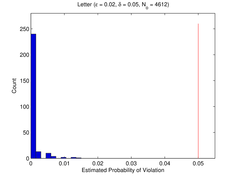
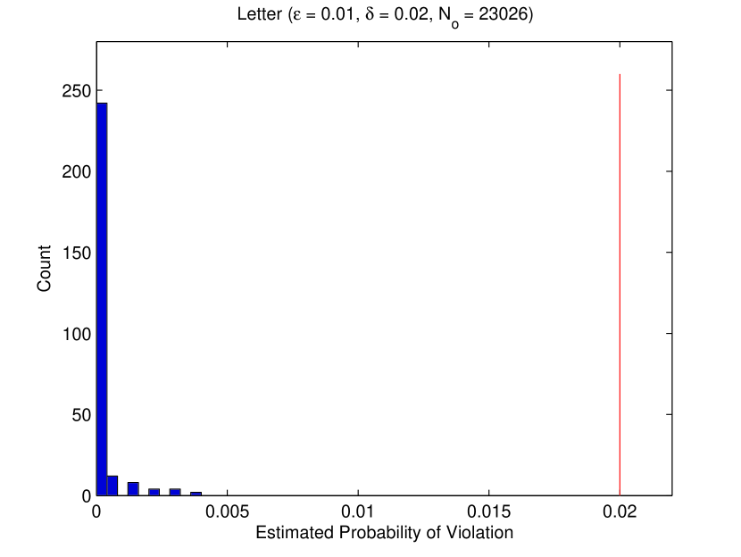
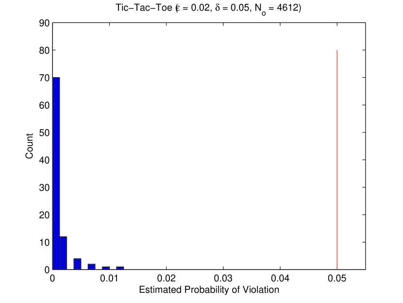
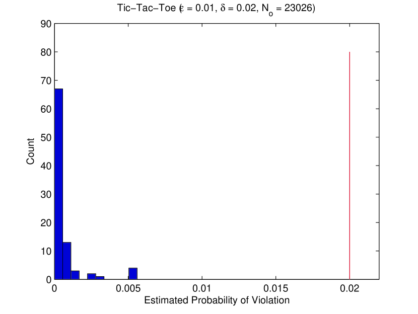
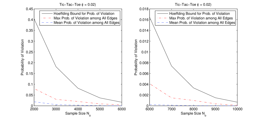
5 Conclusion

We develop new algorithms for efficiently sampling Bayesian network structures (DAGs). The sampled DAGs can then be used to build estimators for the posteriors of any features of interests. Theoretically we show that our estimators have several desirable properties. For example, unlike the existing MCMC algorithms, the estimators based on the DDS algorithm satisfy the Hoeffding bound and therefore enjoy the quality guarantee of the estimation with the given number of samples. Empirically we show that our estimators considerably outperform the previous state-of-the-art with or without assuming the order-modular prior.

Our algorithms are capable of estimating the posteriors of arbitrary (non-modular) features (the DDS under the order-modular prior, the IW-DDS under the structure-modular prior); while the exact algorithms are available for computing modular features under the order-modular prior with time $O(n^{k+1}C(m)+kn2^{n})$ and space $O(n2^{n})$ (Koivisto and Sood, 2004; Koivisto, 2006); computing path features under the order-modular prior with time $O(n^{k+1}C(m)+n3^{n})$ and space $O(3^{n})$ (Parviainen and Koivisto, 2011); and computing modular features under the structure-modular prior with time $O(n^{k+1}C(m)+kn2^{n}+3^{n})$ and space $O(n2^{n})$ (Tian and He, 2009). The bottleneck of our algorithms is their first computation step, the DP algorithm of Koivisto and Sood (2004) whose space cost is $O(n2^{n})$. Therefore the application of our algorithms is limited to the data sets on which the DP algorithm of Koivisto and Sood (2004) is able to run – up to around 25 variables in current desktops, while a parallel implementation of the DP algorithm has been demonstrated on a data set with 33 variables using a cluster including totally 2,048 processors and 8,192 GB memory (Chen et al., 2014).

A Proofs of Propositions, Theorems and Corollary

This appendix provides the proofs of the propositions, theorems and corollary in the paper.

A.1 Proof of Proposition 1

We first prove a lemma for Proposition 1.

Let an order $\prec$ be represented as $(\sigma_{1},\ldots,\sigma_{n})$ where $\sigma_{i}$ is the $i$th element in the order.

Lemma 8

The probability that the last $n-k+1$ elements along the order are $\sigma_{k},\sigma_{k+1},\ldots,\sigma_{n}$ respectively is given by

$$p(\sigma_{k},\sigma_{k+1},\ldots,\sigma_{n},D)=L^{\prime}(U^{\prec}_{\sigma_{k}})\prod_{i=k}^{n}\alpha^{\prime}_{\sigma_{i}}(U^{\prec}_{\sigma_{i}}),$$

where $U^{\prec}_{\sigma_{i}}=V-\{\sigma_{i},\sigma_{i+1},\ldots,\sigma_{n}\}$.

Proof 

$$p(\sigma_{k},\sigma_{k+1},\ldots,\sigma_{n},D)$$

$$=\sum_{\prec^{\prime}\in\mathcal{L}(U^{\prec}_{\sigma_{k}})}p(\prec^{\prime},\sigma_{k},\sigma_{k+1},\ldots,\sigma_{n},D)$$

$$=\prod_{i=k}^{n}\alpha^{\prime}_{\sigma_{i}}(U^{\prec}_{\sigma_{i}})\sum_{\prec^{\prime}\in\mathcal{L}(U^{\prec}_{\sigma_{k}})}\prod_{i\in U^{\prec}_{\sigma_{k}}}\alpha^{\prime}_{i}(U^{\prec}_{i})\quad(\textrm{from (\ref{eq-p_prec_D})})$$

$$=L^{\prime}(U^{\prec}_{\sigma_{k}})\prod_{i=k}^{n}\alpha^{\prime}_{\sigma_{i}}(U^{\prec}_{\sigma_{i}}).\quad(\textrm{from (\ref{eq-L_S})})$$

 

Proposition 1 can be directly proved from the conclusion of Lemma 8 according to the definition of conditional probability.

A.2 Proof of Proposition 2

Proof 

From Proposition 1 and $L^{\prime}(U^{\prec}_{\sigma_{1}}=\emptyset)=1$, we have

$$\prod_{k=1}^{n}p(\sigma_{k}|\sigma_{k+1},\ldots,\sigma_{n},D)$$

$$=\frac{\prod_{i=1}^{n}\alpha^{\prime}_{\sigma_{i}}(U^{\prec}_{\sigma_{i}})}{L^{\prime}(V)}$$

$$=\frac{p(\prec,D)}{p_{\prec}(D)}\quad(\textrm{from (\ref{eq-p_prec_D}) \& (\ref{eq-120330237}) })$$

$$=p(\prec|D),$$

which proves Eq. (20).  

A.3 Proof of Theorem 3

Proof 

First, we show that each DAG $G$ sampled according to our DDS algorithm has its pmf $p_{s}(G)$ equal to the exact posterior $p_{\prec}(G|D)$ by assuming the order-modular prior.

On one hand, from the following derivation, we can get the exact form for $p_{\prec}(G|D)$:

$$p_{\prec}(f|D)$$

$$=\sum_{\prec}p(\prec|D)p(f|\prec,D)$$

$$=\sum_{\prec}p(\prec|D)\sum_{G\subseteq\prec}f(G)p(G|\prec,D)$$

$$=\sum_{\prec}\sum_{G\subseteq\prec}f(G)p(\prec,G|D)$$

$$=\sum_{G}f(G)\sum_{\prec s.t.G\subseteq\prec}p(\prec,G|D).$$ (28)

Thus, for each possible DAG $G_{i}$, by setting $f(G)$ to be the indication function $I[G=G_{i}]$ and then relating Eq. (28) with Eq. (4), we know that $p_{\prec}(G_{i}|D)=\sum_{\prec s.t.G_{i}\subseteq\prec}p(\prec,G_{i}|D)$ for each $G_{i}$.

On the other hand, the event that a DAG $G$ gets sampled according to our DDS algorithm occurs if and only if one of the orders that $G$ is consistent with gets sampled in Step 2 of the DDS algorithm and then $G$ gets sampled from the sampled order in Step 3 of the DDS algorithm. Therefore, based on Total Probability Formula, $p_{s}(G)$ $=\sum_{\prec s.t.G\subseteq\prec}p(\prec|D)p(G|\prec,D)$ $=\sum_{\prec s.t.G\subseteq\prec}p(\prec,G|D)$ $=p_{\prec}(G|D)$.

Second, since $N_{o}$ orders are sampled independently and each DAG per sampled order is sampled independently, $p_{s}(G_{1},G_{2},\ldots,G_{N_{o}}|D)$ $=\prod_{i=1}^{N_{o}}[\sum_{\prec s.t.G\subseteq\prec}p(\prec|D)p(G_{i}|\prec,D)]$ $=\prod_{i=1}^{N_{o}}$ $p_{\prec}(G_{i}|D)$.

Therefore, Theorem 3 is proved.

 

A.4 Proof of Corollary 4

Proof 

For each $G_{i}$ in the DAG set $\{G_{1},$ $G_{2},\ldots,G_{N_{o}}\}$ sampled from the DDS algorithm, $f(G_{i})\in\{0,1\}$. Since $G_{1},$ $G_{2},\ldots,G_{N_{o}}$ are $iid$ with pmf $p_{\prec}(G|D)$ (by Theorem 3), $f(G_{1}),$ $f(G_{2}),\ldots,$ $f(G_{N_{o}})$ are $iid$ with Bernoulli pmf.

For each $G_{i}$, the following is true for $E(f(G_{i}))$, the expectation of $f(G_{i})$.

$$E(f(G_{i}))$$

$$=\sum_{G}f(G)p_{\prec}(G|D)$$

$$=p_{\prec}(f|D).$$

Thus, $f(G_{1}),$ $f(G_{2}),\ldots,f(G_{N_{o}})$ are $iid$ with Bernoulli($p_{\prec}(f|D)$). In other words, $f(G_{1}),$ $f(G_{2}),\ldots,$ $f(G_{N_{o}})$ are independent; and for each $G_{i}$, $P(f(G_{i})=1)=p_{\prec}(f|D)$ and $P(f(G_{i})=0)=1-p_{\prec}(f|D)$.

(i) Proof that $\hat{p}_{\prec}(f|D)$ is an unbiased estimator for $p_{\prec}(f|D)$, that is, $E(\hat{p}_{\prec}(f|D))$ $=p_{\prec}(f|D)$.

$$E\left(\hat{p}_{\prec}(f|D)\right)$$

$$=E\left(\frac{1}{N_{o}}\sum_{i=1}^{N_{o}}f(G_{i})\right)$$

$$=\frac{1}{N_{o}}\sum_{i=1}^{N_{o}}E\left(f(G_{i})\right)$$

$$=\frac{1}{N_{o}}N_{o}p_{\prec}(f|D)$$

$$=p_{\prec}(f|D).$$

(ii) Proof that $\hat{p}_{\prec}(f|D)$ converges almost surely to $p_{\prec}(f|D)$.

Since $f(G_{1}),$ $f(G_{2}),\ldots,f(G_{N_{o}})$ are $iid$ with $E(f(G_{i}))$ $=p_{\prec}(f|D)<\infty$, and since

$$\hat{p}_{\prec}(f|D)=\frac{1}{N_{o}}\sum_{i=1}^{N_{o}}f(G_{i}),$$

based on the Strong Law of Large Numbers (Theorem 5.5.9) (Casella and Berger, 2002), $\hat{p}_{\prec}(f|D)$ converges almost surely to $p_{\prec}(f|D)$ (as $N_{o}\rightarrow\infty$).

Note that, by Theorem 2.5.1 (Athreya and Lahiri, 2006), the property that $\hat{p}_{\prec}(f|D)$ converges almost surely to $p_{\prec}(f|D)$ implies that $\hat{p}_{\prec}(f|D)$ converges in probability to $p_{\prec}(f|D)$, that is, $\hat{p}_{\prec}(f|D)$ is a consistent estimator for $p_{\prec}(f|D)$.

(iii) Proof that if $0<p_{\prec}(f|D)<1$, then the random variable

$$\frac{\sqrt{N_{o}}(\hat{p}_{\prec}(f|D)-p_{\prec}(f|D))}{\sqrt{\hat{p}_{\prec}(f|D)(1-\hat{p}_{\prec}(f|D))}}$$

has a limiting standard normal distribution, denoted by

$$\frac{\sqrt{N_{o}}(\hat{p}_{\prec}(f|D)-p_{\prec}(f|D))}{\sqrt{\hat{p}_{\prec}(f|D)(1-\hat{p}_{\prec}(f|D))}}\longrightarrow^{d}\mathcal{N}(0,1).$$

Since $f(G_{1}),$ $f(G_{2}),\ldots,f(G_{N_{o}})$ are $iid$ with Bernoulli($p_{\prec}(f|D)$), for each $G_{i}$, the following is true for $Var(f(G_{i}))$, the variance of $f(G_{i})$.

$$Var(f(G_{i}))$$

$$=E(f(G_{i}))(1-E(f(G_{i})))$$

$$=p_{\prec}(f|D)(1-p_{\prec}(f|D))$$

$$<\infty.$$

Since $0<p_{\prec}(f|D)<1$, $Var(f(G_{i}))$ is also strictly greater than 0.

Again, we have already known that $E(f(G_{i}))$ $=p_{\prec}(f|D)<\infty$.

Thus, by the Central Limit Theorem (Theorem 5.5.15) (Casella and Berger, 2002),

$$\frac{\sqrt{N_{o}}(\hat{p}_{\prec}(f|D)-E(f(G)))}{\sqrt{Var(f(G))}}\longrightarrow^{d}\mathcal{N}(0,1),$$

that is,

$$\frac{\sqrt{N_{o}}(\hat{p}_{\prec}(f|D)-p_{\prec}(f|D))}{\sqrt{p_{\prec}(f|D)(1-p_{\prec}(f|D))}}\longrightarrow^{d}\mathcal{N}(0,1).$$

Since $\hat{p}_{\prec}(f|D)$ converges in probability to $p_{\prec}(f|D)$, denoted by $\hat{p}_{\prec}(f|D)$ $\longrightarrow^{p}$ $p_{\prec}(f|D)$, by the Continuous Mapping Theorem (Theorem 5.5.4) (Casella and Berger, 2002),

$$\sqrt{\hat{p}_{\prec}(f|D)(1-\hat{p}_{\prec}(f|D))}\longrightarrow^{p}\sqrt{p_{\prec}(f|D)(1-p_{\prec}(f|D))}.$$

Finally, by Slutsky’s Theorem (Theorem 5.5.17) (Casella and Berger, 2002),

$$\frac{\sqrt{N_{o}}(\hat{p}_{\prec}(f|D)-p_{\prec}(f|D))}{\sqrt{\hat{p}_{\prec}(f|D)(1-\hat{p}_{\prec}(f|D))}}\longrightarrow^{d}\mathcal{N}(0,1).$$

(iv) Proof that for any $\epsilon>0$, any $0<\delta<1$, if $N_{o}\geq(\ln(2/\delta))/(2\epsilon^{2})$, then $p(|\hat{p}_{\prec}(f|D)-p_{\prec}(f|D)|<\epsilon)$ $\geq 1-\delta$.

Since $f(G_{1}),$ $f(G_{2}),\ldots,f(G_{N_{o}})$ are $iid$ with Bernoulli($p_{\prec}(f|D)$), the Hoeffding bound (Hoeffding, 1963; Koller and Friedman, 2009) holds:

$$p(|\hat{p}_{\prec}(f|D)-p_{\prec}(f|D)|\geq\epsilon)\leq 2e^{-2N_{o}\epsilon^{2}}.$$

This is equivalent to

$$p(|\hat{p}_{\prec}(f|D)-p_{\prec}(f|D)|<\epsilon)\geq 1-2e^{-2N_{o}\epsilon^{2}},$$

and the conclusion is implied straightforward.

 

A.5 Proof of Equation (21)

Proof  For any $j$ $\in\{1,\ldots,n\}$:

$$P((\sigma_{j},U_{\sigma_{j}})|D)$$

$$\propto P((\sigma_{j},U_{\sigma_{j}}),D)$$

$$=\sum_{\begin{subarray}{c}(\sigma_{1},\ldots,\sigma_{j-1})\\ \in\mathcal{L}(U_{\sigma_{j}})\end{subarray}}\sum_{\begin{subarray}{c}(\sigma_{j+1},\ldots,\sigma_{n})\\ \in\mathcal{L}(V-U_{\sigma_{j}}-\{\sigma_{j}\})\end{subarray}}P(\sigma_{1},\ldots,\sigma_{j-1},\sigma_{j},\sigma_{j+1},\ldots,\sigma_{n},D)$$

$$=\sum_{\begin{subarray}{c}(\sigma_{1},\ldots,\sigma_{j-1})\\ \in\mathcal{L}(U_{\sigma_{j}})\end{subarray}}\sum_{\begin{subarray}{c}(\sigma_{j+1},\ldots,\sigma_{n})\\ \in\mathcal{L}(V-U_{\sigma_{j}}-\{\sigma_{j}\})\end{subarray}}\prod_{i=1}^{n}\alpha^{\prime}_{\sigma_{i}}(U_{\sigma_{i}})$$

$$=\alpha^{\prime}_{\sigma_{j}}(U_{\sigma_{j}})L^{\prime}(U_{\sigma_{j}})R^{\prime}(V-U_{\sigma_{j}}-\{\sigma_{j}\}).$$

 

A.6 Proof of Equation (22)

Proof 

$$p_{\prec}(G|D)$$

$$=\sum_{\prec s.t.G\subseteq\prec}p(\prec,G|D)$$

$$=\frac{1}{p_{\prec}(D)}\sum_{\prec s.t.G\subseteq\prec}p(\prec,G,D)$$

$$=\frac{1}{p_{\prec}(D)}\sum_{\prec s.t.G\subseteq\prec}p(\prec,G)p(D|G)$$

$$=\frac{1}{p_{\prec}(D)}\sum_{\prec s.t.G\subseteq\prec}(\prod_{i=1}^{n}q_{i}(U_{i})\rho_{i}(Pa_{i}))p(D|G)$$

$$=\frac{1}{p_{\prec}(D)}\sum_{\prec s.t.G\subseteq\prec}(\prod_{i=1}^{n}p_{i}(Pa_{i}))p(D|G)$$

$$=\frac{1}{p_{\prec}(D)}\sum_{\prec s.t.G\subseteq\prec}p(G)p(D|G)$$

$$=\frac{1}{p_{\prec}(D)}\cdot|\prec_{G}|\cdot p_{\nprec}(G,D)$$

$$=\frac{p_{\nprec}(D)}{p_{\prec}(D)}\cdot|\prec_{G}|\cdot p_{\nprec}(G|D).$$

Since both $p_{\nprec}(D)>0$ and $p_{\prec}(D)>0$, $p_{\prec}(G|D)\propto$ $|\prec_{G}|\cdot p_{\nprec}(G|D)$, which also has been shown by Ellis and Wong (2008).

 

A.7 Proof of Theorem 6

Proof 

Let $\Omega$ denote the set of all the DAGs. Define $\mathcal{U}^{+}$ $=$ $\{G\in\Omega:p_{\nprec}(G,D)>0\}$. $\mathcal{U}^{+}$ will equal $\Omega$ if the user chooses a prior such that $p(G)>0$ for every DAG $G$ (such as a uniform DAG prior $p(G)\equiv 1$). However, if the user has some additional domain knowledge so that he/she sets some prior to exclude some DAGs a priori, $\mathcal{U}^{+}$ will be a proper subset of $\Omega$. Note that $p_{\nprec}(f|D)$ $=p_{\nprec}(f,D)/p_{\nprec}(D)$, where $p_{\nprec}(f,D)$ $=\sum_{G}f(G)p_{\nprec}(G,D)$ $=\sum_{G\in\mathcal{U}^{+}}f(G)p_{\nprec}(G,D)$, and $p_{\nprec}(D)$ $=p_{\nprec}(f\equiv 1,D)$ $=\sum_{G}p_{\nprec}(G,D)$ $=\sum_{G\in\mathcal{U}^{+}}p_{\nprec}(G,D)$.

Let $I[]$ denote the indicator function. Rewrite $\hat{p}_{\nprec}(f|D)$ in Eq. (24) as $\hat{p}_{\nprec}(f,D)/\hat{p}_{\nprec}(D)$, where $\hat{p}_{\nprec}(f,D)$ $=\sum_{G\in\mathcal{G}}f(G)p_{\nprec}(G,D)$ $=\sum_{G}f(G)$ $p_{\nprec}(G,D)I[G\in\mathcal{G}]$ $=\sum_{G\in\mathcal{U}^{+}}f(G)p_{\nprec}(G,D)I[$ $G\in\mathcal{G}]$, and $\hat{p}_{\nprec}(D)$ $=\hat{p}_{\nprec}(f\equiv 1,D)$ $=\sum_{G\in\mathcal{G}}p_{\nprec}(G,D)$ $=\sum_{G}p_{\nprec}(G,D)I[G\in\mathcal{G}]$ $=\sum_{G\in\mathcal{U}^{+}}$ $p_{\nprec}(G,D)I[G\in\mathcal{G}]$.

Note that by Theorem 3, $P(G\in\mathcal{G})$ = $1-(1-p_{\prec}(G|D))^{N_{o}}$, where $p_{\prec}(G|D)$ is the exact posterior of $G$ under the order-modular prior assumption. Also note that by Eq. (22), $\forall G:(p_{\nprec}(G,D)>0)\Rightarrow(p_{\prec}(G|D)>0)$.

(i) Proof that $\hat{p}_{\nprec}(f|D)$ is an asymptotically unbiased estimator for $p_{\nprec}(f|D)$, that is,

$$\lim_{N_{o}\to\infty}E(\hat{p}_{\nprec}(f|D))=p_{\nprec}(f|D).$$ (29)

For notational convenience, let $\gamma$ denote $\hat{p}_{\nprec}(f,D)$, and let $\tau$ denote $\hat{p}_{\nprec}(D)$. Define $g(\gamma,\tau)$ $=\gamma/\tau$ so that $g(\gamma,\tau)$ is essentially $\hat{p}_{\nprec}(f|D)$.

Note that

$$E(\gamma)$$

$$=E(\hat{p}_{\nprec}(f,D))$$

$$=E\left(\sum_{G\in\mathcal{U}^{+}}f(G)p_{\nprec}(G,D)I[G\in\mathcal{G}]\right)$$

$$=\sum_{G\in\mathcal{U}^{+}}E(f(G)p_{\nprec}(G,D)I[G\in\mathcal{G}])$$

$$=\sum_{G\in\mathcal{U}^{+}}f(G)p_{\nprec}(G,D)P(G\in\mathcal{G})$$

$$=\sum_{G\in\mathcal{U}^{+}}f(G)p_{\nprec}(G,D)(1-(1-p_{\prec}(G|D))^{N_{o}}).$$

Thus,

$$\lim_{N_{o}\to\infty}E(\gamma)$$

$$=\lim_{N_{o}\to\infty}\left(\sum_{G\in\mathcal{U}^{+}}f(G)p_{\nprec}(G,D)(1-(1-p_{\prec}(G|D))^{N_{o}})\right)$$

$$=\sum_{G\in\mathcal{U}^{+}}f(G)p_{\nprec}(G,D)\lim_{N_{o}\to\infty}(1-(1-p_{\prec}(G|D))^{N_{o}})$$

$$=\sum_{G\in\mathcal{U}^{+}}f(G)p_{\nprec}(G,D)$$

$$=p_{\nprec}(f,D).$$

Similarly, by setting $f\equiv 1$, we have

$$E(\tau)$$

$$=E(\hat{p}_{\nprec}(D))$$

$$=\sum_{G\in\mathcal{U}^{+}}p_{\nprec}(G,D)(1-(1-p_{\prec}(G|D))^{N_{o}}),$$

and

$$\lim_{N_{o}\to\infty}E(\tau)=p_{\nprec}(D).$$

Next, by Taylor’s Theorem (with the Lagrange form of the remainder),

$$g(\gamma,\tau)$$

$$=g(E(\gamma),E(\tau))+\left[\frac{\partial g(\gamma,\tau)}{\partial\gamma}\right]_{\gamma=E(\gamma),\tau=E(\tau)}(\gamma^{*}-E(\gamma))$$

$$\;\;\;\;+\left[\frac{\partial g(\gamma,\tau)}{\partial\tau}\right]_{\gamma=E(\gamma),\tau=E(\tau)}(\tau^{*}-E(\tau)),$$

where $\gamma^{*}$ $=E(\gamma)+\theta(\gamma-E(\gamma))$, $\tau^{*}$ $=E(\tau)+\theta(\tau-E(\tau))$, and $\theta$ is a random variable such that $0<\theta<1$.

Examine the components separately:

$$g(E(\gamma),E(\tau))=E(\gamma)/E(\tau).$$

$$\left[\frac{\partial g(\gamma,\tau)}{\partial\gamma}\right]_{\gamma=E(\gamma),\tau=E(\tau)}$$

$$=\left[\tau^{-1}\right]_{\gamma=E(\gamma),\tau=E(\tau)}$$

$$=(E(\tau))^{-1}.$$

$$\left[\frac{\partial g(\gamma,\tau)}{\partial\tau}\right]_{\gamma=E(\gamma),\tau=E(\tau)}$$

$$=\left[-\gamma(\tau)^{-2}\right]_{\gamma=E(\gamma),\tau=E(\tau)}$$

$$=-E(\gamma)(E(\tau))^{-2}.$$

Since neither $E(\gamma)$ nor $E(\tau)$ is random,

$$E\left(g(\gamma,\tau)\right)$$

$$=E(\gamma)/E(\tau)+(E(\tau))^{-1}E(\gamma^{*}-E(\gamma))-E(\gamma)(E(\tau))^{-2}E(\tau^{*}-E(\tau))$$

$$=E(\gamma)/E(\tau)+(E(\tau))^{-1}E(\theta(\gamma-E(\gamma)))-E(\gamma)(E(\tau))^{-2}E(\theta(\tau-E(\tau))).$$

Consider the limit of each component separately:

$$\lim_{N_{o}\to\infty}\left(E(\gamma)/E(\tau)\right)$$

$$=\left(\lim_{N_{o}\to\infty}E(\gamma)\right)/\left(\lim_{N_{o}\to\infty}E(\tau)\right)$$

$$=p_{\nprec}(f,D)/p_{\nprec}(D)$$

$$=p_{\nprec}(f|D).$$

$$\lim_{N_{o}\to\infty}(E(\tau))^{-1}$$

$$=\left(\lim_{N_{o}\to\infty}E(\tau)\right)^{-1}$$

$$=(p_{\nprec}(D))^{-1}.$$

$$\lim_{N_{o}\to\infty}-E(\gamma)(E(\tau))^{-2}$$

$$=-\left(\lim_{N_{o}\to\infty}E(\gamma)\right)\left(\lim_{N_{o}\to\infty}E(\tau)\right)^{-2}$$

$$=-p_{\nprec}(f,D)(p_{\nprec}(D))^{-2}.$$

Note that both $(p_{\nprec}(D))^{-1}$ and $-p_{\nprec}(f,D)(p_{\nprec}(D))^{-2}$ are constant real numbers.

Finally, we intend to prove the following two equalities:

$$\lim_{N_{o}\to\infty}E(\theta(\gamma-E(\gamma)))=0,$$ (30)

$$\lim_{N_{o}\to\infty}E(\theta(\tau-E(\tau)))=0.$$ (31)

Once this is done,

$$\lim_{N_{o}\to\infty}E\left(g(\gamma,\tau)\right)$$

$$=\lim_{N_{o}\to\infty}\left(E(\gamma)/E(\tau)\right)+\lim_{N_{o}\to\infty}(E(\tau))^{-1}\cdot 0+\lim_{N_{o}\to\infty}\left(-E(\gamma)(E(\tau))^{-2}\right)\cdot 0$$

$$=p_{\nprec}(f|D).$$

The whole proof for Eq. (29) will then be done.

The proof for Eq. (30) is as follows.

Based on the definition of limit, proving Eq. (30) is equivalent to proving

$$\lim_{N_{o}\to\infty}\left|E(\theta(\gamma-E(\gamma)))\right|=0.$$ (32)

Since

$$\left|E(\theta(\gamma-E(\gamma)))\right|$$

$$\leq E\left(|\theta(\gamma-E(\gamma))|\right)$$

$$=E\left(|\theta|\cdot|\gamma-E(\gamma)|\right)$$

$$\leq E\left(|\gamma-E(\gamma)|\right)\quad(\textrm{due to $0<\theta<1$ }),$$

and $\left|E(\theta(\gamma-E(\gamma)))\right|\geq 0$, to prove Eq. (32), it is sufficient to prove

$$\lim_{N_{o}\to\infty}E\left(|\gamma-E(\gamma)|\right)=0.$$ (33)

$$E\left(|\gamma-E(\gamma)|\right)$$

$$=E\left(\left|\sum_{G\in\mathcal{U}^{+}}f(G)p_{\nprec}(G,D)I[G\in\mathcal{G}]\right.\right.\left.\left.-\sum_{G\in\mathcal{U}^{+}}f(G)p_{\nprec}(G,D)P(G\in\mathcal{G})\right|\right)$$

$$=E\left(\left|\sum_{G\in\mathcal{U}^{+}}f(G)p_{\nprec}(G,D)(I[G\in\mathcal{G}]-P(G\in\mathcal{G}))\right|\right)$$

$$\leq E\left(\sum_{G\in\mathcal{U}^{+}}f(G)p_{\nprec}(G,D)\left|I[G\in\mathcal{G}]-P(G\in\mathcal{G})\right|\right)$$

$$=\sum_{G\in\mathcal{U}^{+}}f(G)p_{\nprec}(G,D)E\left(\left|I[G\in\mathcal{G}]-P(G\in\mathcal{G})\right|\right)$$

$$=\sum_{G\in\mathcal{U}^{+}}f(G)p_{\nprec}(G,D)[(1-P(G\in\mathcal{G}))P(G\in\mathcal{G})$$

$$\;\;\;\;\;\;\;\;\;\;+(P(G\in\mathcal{G})-0)(1-P(G\in\mathcal{G}))]$$

$$=\sum_{G\in\mathcal{U}^{+}}f(G)p_{\nprec}(G,D)[2P(G\in\mathcal{G})(1-P(G\in\mathcal{G}))]$$

$$=\sum_{G\in\mathcal{U}^{+}}f(G)p_{\nprec}(G,D)[2(1-(1-p_{\prec}(G|D))^{N_{o}})\times(1-p_{\prec}(G|D))^{N_{o}}].$$

Since $\forall G\in\mathcal{U}^{+}:p_{\prec}(G|D)>0$,

$$\lim_{N_{o}\to\infty}\sum_{G\in\mathcal{U}^{+}}f(G)p_{\nprec}(G,D)[2(1-(1-p_{\prec}(G|D))^{N_{o}})\times(1-p_{\prec}(G|D))^{N_{o}}]$$

$$=\sum_{G\in\mathcal{U}^{+}}f(G)p_{\nprec}(G,D)\lim_{N_{o}\to\infty}[2(1-(1-p_{\prec}(G|D))^{N_{o}})\times(1-p_{\prec}(G|D))^{N_{o}}]$$

$$=\sum_{G\in\mathcal{U}^{+}}f(G)p_{\nprec}(G,D)\cdot 0$$

$$=0,$$

Eq. (33) is proved, and the proof for Eq. (30) is done.

Setting $f\equiv 1$ in Eq. (30) leads to Eq. (31).

Thus, the whole proof for Eq. (29) is done.

(ii) Proof that $\hat{p}_{\nprec}(f|D)$ converges almost surely to $p_{\nprec}(f|D)$, denoted by $\hat{p}_{\nprec}(f|D)\longrightarrow^{a.s.}p_{\nprec}(f|D)$.

Remember that $\Omega$ denotes the set of all the DAGs, that is, $\Omega$ $=\{G_{1},G_{2},\ldots,G_{W^{*}}\}$, where $W^{*}$ is $|\Omega|$, the number of all the DAGs. Note that $W^{*}$ is a finite positive integer though it is super-exponential in the number of variables $n$.

Let $\mathcal{F}$ be $\mathcal{P}(\Omega)$, the power set of $\Omega$. Thus, $\mathcal{F}$ is a $\sigma-$algebra on $\Omega$ (Athreya and Lahiri, 2006). Define for any $A\in\mathcal{F}$, $\mu(A)$ $=\sum_{G_{j}\in A}p_{\prec}(G_{j}|D)$. It is well-known that $\mu$ is a probability measure on $\mathcal{F}$ so that $(\Omega,\mathcal{F},\mu)$ is a probability space (Athreya and Lahiri, 2006).

For each $i\geq 1$, let $\Omega_{i}=\Omega$, $\mathcal{F}_{i}=\mathcal{F}$ and $\mu_{i}=\mu$. Let $\Omega^{\infty}$ $=\{(G^{(1)},G^{(2)},\ldots):G^{(i)}\in\Omega_{i},i\geq 1\}$. Let a cylinder set $\uwave{A}=$ $A_{1}\times A_{2}\times\ldots\times A_{k}\times\Omega_{k+1}\times\Omega_{k+2}\times\ldots$, where there exists $1\leq k<\infty$ such that $A_{i}\in\mathcal{F}_{i}$ for $1\leq i\leq k$ and $A_{i}=\Omega_{i}$ for $i>k$. Let $\mathcal{F}^{\infty}$ $=\sigma<\{\uwave{A}:\uwave{A}$ is a cylinder set $\}>$, that is, $\mathcal{F}^{\infty}$ is a $\sigma-$algebra generated by the set of all the $\uwave{A}$’s. $\mathcal{F}^{\infty}$ is a a $\sigma-$algebra on $\Omega^{\infty}$ and is called a product $\sigma-$algebra.

Define, for each $(A_{1},A_{2},\ldots,A_{k},\Omega_{k+1},\Omega_{k+2},\ldots)\in\mathcal{F}^{\infty}$, $\mu^{\infty}(A_{1},A_{2},\ldots,A_{k},\Omega_{k+1},\Omega_{k+2},$ $\ldots)$ $=\mu_{1}(A_{1})\times\mu_{2}(A_{2})\times\ldots\times\mu_{k}(A_{k})$. By Kolmogorov’s consistency theorem, $(\Omega^{\infty},\mathcal{F}^{\infty},\mu^{\infty})$ is a probability space (Athreya and Lahiri, 2006).

Let $\Omega^{\infty,0}$ $=\{(G^{(1)},G^{(2)},\ldots)\in\Omega^{\infty}:\exists G\in\mathcal{U}^{+}:\forall i\geq 1:G^{(i)}\neq G\}$. Let $\Omega^{\infty,1}$ $=\Omega^{\infty}-\Omega^{\infty,0}$. Thus, $\Omega^{\infty,1}$ $=\{(G^{(1)},G^{(2)},\ldots)\in\Omega^{\infty}:\forall G\in\mathcal{U}^{+}:\exists i\geq 1:G^{(i)}=G\}$.

Define, for each $\omega^{\infty}\in\Omega^{\infty}$,

$$\hat{p}_{\nprec}^{N_{o}}(\omega^{\infty})=\frac{\sum_{G\in\mathcal{U}^{+}}f(G)p_{\nprec}(G,D)I[G\in\mathcal{G}^{N_{o}}(\omega^{\infty})]}{\sum_{G\in\mathcal{U}^{+}}p_{\nprec}(G,D)I[G\in\mathcal{G}^{N_{o}}(\omega^{\infty})]},$$

where $\mathcal{G}^{N_{o}}(\omega^{\infty})$ is the DAG set including the first $N_{o}$ coordinates of $\omega^{\infty}$. By the definition, we know that $\hat{p}_{\nprec}^{N_{o}}(\omega^{\infty})$ $=\hat{p}_{\nprec}(f|D)$.

For each $\omega^{\infty}\in\Omega^{\infty,1}$, for each $G\in\mathcal{U}^{+}$, let $N(G,\omega^{\infty})$ be the smallest integer such that $G^{(N(G,\omega^{\infty}))}=G$. Let $N(\omega^{\infty})$ $=max_{G\in\mathcal{U}^{+}}N(G,\omega^{\infty})$. Then for each $N_{o}\geq N(\omega^{\infty})$, for each $G\in\mathcal{U}^{+}$, $I[G\in\mathcal{G}^{N_{o}}(\omega^{\infty})]$ $=1$.

Accordingly, for each $\omega^{\infty}\in\Omega^{\infty,1}$, there exists $N(\omega^{\infty})$ such that for each $N_{o}\geq N(\omega^{\infty})$:

$$\hat{p}_{\nprec}^{N_{o}}(\omega^{\infty})$$

$$=\frac{\sum_{G\in\mathcal{U}^{+}}f(G)p_{\nprec}(G,D)}{\sum_{G\in\mathcal{U}^{+}}p_{\nprec}(G,D)}$$

$$=p_{\nprec}(f|D).$$

This implies that $\lim_{N_{o}\to\infty}\hat{p}_{\nprec}^{N_{o}}(\omega^{\infty})=p_{\nprec}(f|D)$ for each $\omega^{\infty}\in\Omega^{\infty,1}$.

Finally, we intend to prove the following equality:

$$\mu^{\infty}(\Omega^{\infty,1})=1.$$ (34)

Once this is done, the whole proof for $\hat{p}_{\nprec}(f|D)$ $\longrightarrow^{a.s.}p_{\nprec}(f|D)$ is done.

Proving Eq. (34) is equivalent to proving

$$\mu^{\infty}(\Omega^{\infty,0})=0.$$ (35)

For any $G\in\Omega$, let $\Omega^{\infty,0,G}$ $=\{(G^{(1)},G^{(2)},\ldots)\in\Omega^{\infty}:\forall i\geq 1:G^{(i)}\neq G\}$. Thus, $\Omega^{\infty,0}$ $=\bigcup_{G\in\mathcal{U}^{+}}\Omega^{\infty,0,G}$. Accordingly, $\mu^{\infty}(\Omega^{\infty,0})$ $\leq\sum_{G\in\mathcal{U}^{+}}\mu^{\infty}(\Omega^{\infty,0,G})$.

For each $j\geq 1$, let $\Omega^{\infty,0,G,j}$ $=\{(G^{(1)},G^{(2)},\ldots)\in\Omega^{\infty}:\forall i\in\{1,\ldots,j\}:G^{(i)}\neq G\}$. Note $\Omega^{\infty,0,G,1}$ $\supseteq\Omega^{\infty,0,G,2}$ $\supseteq\ldots$ $\supseteq\Omega^{\infty,0,G,j-1}$ $\supseteq\Omega^{\infty,0,G,j}$ for each $j\geq 1$. Thus, $\Omega^{\infty,0,G}$ $=\bigcap_{j=1}^{\infty}\Omega^{\infty,0,G,j}$.

Finally, for any $G\in\mathcal{U}^{+}$,

$$\mu^{\infty}(\Omega^{\infty,0,G})$$

$$=\mu^{\infty}(\bigcap_{j=1}^{\infty}\Omega^{\infty,0,G,j})$$

$$=\lim_{j\to\infty}\mu^{\infty}(\Omega^{\infty,0,G,j})$$

$$=\lim_{j\to\infty}\mu_{1}(\Omega-\{G\})\times\mu_{2}(\Omega-\{G\})\times\ldots\times\mu_{j}(\Omega-\{G\})$$

$$=\lim_{j\to\infty}[1-\mu(\{G\})]^{j}$$

$$=\lim_{j\to\infty}[1-p_{\prec}(G|D)]^{j}$$

$$=0.$$

Thus, $\sum_{G\in\mathcal{U}^{+}}\mu^{\infty}(\Omega^{\infty,0,G})=0$, so that Eq. (35) is proved. The whole proof is done.

Note that, by Theorem 2.5.1 (Athreya and Lahiri, 2006), the property that $\hat{p}_{\nprec}(f|D)$ converges almost surely to $p_{\nprec}(f|D)$ implies that $\hat{p}_{\nprec}(f|D)$ converges in probability to $p_{\nprec}(f|D)$, that is, $\hat{p}_{\nprec}(f|D)$ is a consistent estimator for $p_{\nprec}(f|D)$.

(iii) Proof that the convergence rate of $\hat{p}_{\nprec}(f|D)$ is $o(a^{N_{o}})$ for any $0<a<1$.

In the proof for (ii), we have shown that for each $\omega^{\infty}\in\Omega^{\infty,1}$, there exists $N(\omega^{\infty})$ such that for each $N_{o}\geq N(\omega^{\infty})$, $\hat{p}_{\nprec}^{N_{o}}(\omega^{\infty})=p_{\nprec}(f|D)$. This means that for any $0<a<1$, $(a^{N_{o}})^{-1}[\hat{p}_{\nprec}^{N_{o}}(\omega^{\infty})-p_{\nprec}(f|D)]=0$. Thus, $\lim_{N_{o}\to\infty}(a^{N_{o}})^{-1}[\hat{p}_{\nprec}^{N_{o}}(\omega^{\infty})-p_{\nprec}(f|D)]=0$ so that the proof is done.

(iv) Proof that if the quantity $\Delta=\sum_{G\in\mathcal{G}}p_{\nprec}(G|D)$, then $\Delta\cdot\hat{p}_{\nprec}(f|D)\leq p_{\nprec}(f|D)\leq\Delta\cdot\hat{p}_{\nprec}(f|D)+1-\Delta$.

The proof is essentially the same as the proof for Proposition 1 of Tian et al. (2010) which proves Eq. (27), an equivalent form of Eq. (26). The direct proof for Eq. (26) is also provided in the supplementary material.

References

- Asuncion and Newman (2007) Arthur Asuncion and David J Newman. UCI machine learning repository, 2007.
- Athreya and Lahiri (2006) Krishna B. Athreya and Soumendra N. Lahiri. Measure Theory and Probability Theory. Springer, 2006.
- Binder et al. (1997) John Binder, Daphne Koller, Stuart Russell, and Keiji Kanazawa. Adaptive probabilistic networks with hidden variables. Machine Learning, 29(2-3):213–244, 1997.
- Brightwell and Winkler (1991) Graham Brightwell and Peter Winkler. Counting linear extensions is #P-complete. In Proceedings of the twenty-third annual ACM symposium on Theory of computing, pages 175–181, 1991.
- Casella and Berger (2002) George Casella and Roger L. Berger. Statistical Inference. Duxbury, 2002.
- Chen et al. (2014) Yetian Chen, Jin Tian, Olga Nikolova, and Srinivas Aluru. A parallel algorithm for exact Bayesian structure discovery in Bayesian networks. CoRR, abs/1408.1664, 2014. URL http://arxiv.org/abs/1408.1664.
- Cooper and Herskovits (1992) Gregory F. Cooper and Edward Herskovits. A Bayesian method for the induction of probabilistic networks from data. Machine Learning, 9:309–347, 1992.
- Cussens (2011) James Cussens. Bayesian network learning with cutting planes. In Proceedings of the Conference on Uncertainty in Artificial Intelligence (UAI), pages 153–160, 2011.
- Cussens and Bartlett (2013) James Cussens and Mark Bartlett. Advances in Bayesian network learning using integer programming. In Proceedings of the Conference on Uncertainty in Artificial Intelligence (UAI), pages 182 – 191, 2013.
- Dash and Cooper (2004) Denver Dash and Gregory F. Cooper. Model averaging for prediction with discrete Bayesian networks. Journal of Machine Learning Research, 5:1177–1203, 2004.
- Eaton and Murphy (2007) Daniel Eaton and Kevin Murphy. Bayesian structure learning using dynamic programming and MCMC. In Proceedings of the Conference on Uncertainty in Artificial Intelligence (UAI), pages 101–108, 2007.
- Edwards (2000) David Edwards. Introduction to Graphical Modelling. Springer, 2nd edition, 2000.
- Ellis and Wong (2008) Byron Ellis and Wing H. Wong. Learning causal Bayesian network structures from experimental data. Journal of the American Statistical Association, 103:778–789, 2008.
- Flerova et al. (2012) Natalia Flerova, Emma Rollon, and Rina Dechter. Bucket and mini-bucket schemes for m best solutions over graphical models. In Graph Structures for Knowledge Representation and Reasoning, volume 7205, pages 91–118. 2012.
- Friedman and Koller (2003) Nir Friedman and Daphne Koller. Being Bayesian about network structure: A Bayesian approach to structure discovery in Bayesian networks. Machine Learning, 50(1-2):95–125, 2003.
- Friedman et al. (1999) Nir Friedman, Moises Goldszmidt, and Abraham Wyner. Data analysis with Bayesian networks: A bootstrap approach. In Proceedings of the Conference on Uncertainty in Artificial Intelligence (UAI), pages 196–205, 1999.
- Grzegorczyk and Husmeier (2008) Marco Grzegorczyk and Dirk Husmeier. Improving the structure MCMC sampler for Bayesian networks by introducing a new edge reversal move. Machine Learning, 71:265–305, 2008.
- Heckerman et al. (1995) David Heckerman, Dan Geiger, and David M. Chickering. Learning Bayesian networks: The combination of knowledge and statistical data. Machine Learning, 20:197–243, 1995.
- Heckerman et al. (1999) David Heckerman, Christopher Meek, and Gregory Cooper. A Bayesian approach to causal discovery. In C. Glymour and G.F. Cooper, editors, Computation, Causation, and Discovery, pages 141–165, 1999.
- Hoeffding (1963) Wassily Hoeffding. Probability inequalities for sums of bounded random variables. Journal of the American Statistical Association, 58(301):pp. 13–30, 1963.
- Jaakkola et al. (2010) Tommi Jaakkola, David Sontag, Amir Globerson, and Marina Meila. Learning Bayesian network structure using LP relaxations. In Proceedings of the International Conference on Artificial Intelligence and Statistics (AISTATS), pages 358 – 365, 2010.
- Jerrum et al. (1986) Mark R. Jerrum, Leslie G. Valiant, and Vijay V. Vazirani. Random generation of combinatorial structures from a uniform distribution. Theoretical Computer Science, 43:169 – 188, 1986.
- Kennes and Smets (1991) Robert Kennes and Philippe Smets. Computational aspects of the Möbius transformation. In Proceedings of the Conference on Uncertainty in Artificial Intelligence (UAI), pages 401–416, 1991.
- Koivisto (2006) Mikko Koivisto. Advances in exact Bayesian structure discovery in Bayesian networks. In Proceedings of the Conference on Uncertainty in Artificial Intelligence (UAI), pages 241–248, 2006.
- Koivisto and Sood (2004) Mikko Koivisto and Kismat Sood. Exact Bayesian structure discovery in Bayesian networks. Journal of Machine Learning Research, 5:549–573, 2004.
- Koller and Friedman (2009) Daphne Koller and Nir Friedman. Probabilistic Graphical Models: Principles and Techniques. The MIT Press, 2009.
- Madigan and York (1995) David Madigan and Jeremy York. Bayesian graphical models for discrete data. International Statistical Review, 63:215–232, 1995.
- Malone and Yuan (2013) Brandon Malone and Changhe Yuan. Evaluating anytime algorithms for learning optimal Bayesian networks. In Proceedings of the Conference on Uncertainty in Artificial Intelligence (UAI), pages 381 – 390, 2013.
- Malone et al. (2011a) Brandon Malone, Changhe Yuan, and Eric Hansen. Memory-efficient dynamic programming for learning optimal Bayesian networks. In Proceedings of the AAAI Conference on Artificial Intelligence (AAAI), pages 1057 – 1062, 2011a.
- Malone et al. (2011b) Brandon Malone, Changhe Yuan, Eric A Hansen, and Susan Bridges. Improving the scalability of optimal Bayesian network learning with external-memory frontier breadth-first branch and bound search. In Proceedings of the Conference on Uncertainty in Artificial Intelligence (UAI), pages 479–488, 2011b.
- Meila and Jaakkola (2006) Marina Meila and Tommi Jaakkola. Tractable Bayesian learning of tree belief networks. Statistics and Computing, 16:77–92, 2006.
- Niinimaki and Koivisto (2013) Teppo Niinimaki and Mikko Koivisto. Annealed importance sampling for structure learning in Bayesian networks. In Proceedings of the International Joint Conference on Artificial Intelligence (IJCAI), pages 1579–1585, 2013.
- Niinimaki et al. (2011) Teppo Niinimaki, Pekka Parviainen, and Mikko Koivisto. Partial order MCMC for structure discovery in Bayesian networks. In Proceedings of the Conference on Uncertainty in Artificial Intelligence (UAI), pages 557–564, 2011.
- Parviainen and Koivisto (2010) Pekka Parviainen and Mikko Koivisto. Bayesian structure discovery in Bayesian networks with less space. In Proceedings of the International Conference on Artificial Intelligence and Statistics (AISTATS), pages 589–596, 2010.
- Parviainen and Koivisto (2011) Pekka Parviainen and Mikko Koivisto. Ancestor relations in the presence of unobserved variables. In Proceedings of the European conference on machine learning and knowledge discovery in databases (ECML PKDD), pages 581–596, 2011.
- Pearl (2000) Judea Pearl. Causality: Models, Reasoning, and Inference. Cambridge University Press, NY, 2000.
- Silander and Myllymaki (2006) Tomi Silander and Petri Myllymaki. A simple approach for finding the globally optimal Bayesian network structure. In Proceedings of the Conference on Uncertainty in Artificial Intelligence (UAI), pages 445–452, 2006.
- Spirtes et al. (2001) Peter Spirtes, Clark Glymour, and Richard Scheines. Causation, Prediction, and Search (2nd Edition). MIT Press, Cambridge, MA, 2001.
- Tian and He (2009) Jin Tian and Ru He. Computing posterior probabilities of structural features in Bayesian networks. In Proceedings of the Conference on Uncertainty in Artificial Intelligence (UAI), pages 538–547, 2009.
- Tian et al. (2010) Jin Tian, Ru He, and Lavanya Ram. Bayesian model averaging using the k-best Bayesian network structures. In Proceedings of the Conference on Uncertainty in Artificial Intelligence (UAI), pages 589–597, 2010.
- Tsamardinos et al. (2006) Ioannis Tsamardinos, Laura Brown, and Constantin Aliferis. The max-min hill-climbing Bayesian network structure learning algorithm. Machine Learning, 65:31–78, 2006.
- Yuan and Malone (2012) Changhe Yuan and Brandon Malone. An improved admissible heuristic for learning optimal Bayesian networks. In Proceedings of the Conference on Uncertainty in Artificial Intelligence (UAI), pages 924–933, 2012.
- Yuan and Malone (2013) Changhe Yuan and Brandon Malone. Learning optimal Bayesian networks: A shortest path perspective. Journal of Artificial Intelligence Research (JAIR), 48:23 – 65, 2013.
- Yuan et al. (2011) Changhe Yuan, Brandon Malone, and Xiaojian Wu. Learning optimal Bayesian networks using A* search. In Proceedings of the International Joint Conference on Artificial Intelligence (IJCAI), pages 2186–2191, 2011.