Entanglement entropy and negativity of disjoint intervals in CFT: Some numerical extrapolations

Abstract

The entanglement entropy and the logarithmic negativity can be computed in quantum field theory through a method based on the replica limit. Performing these analytic continuations in some cases is beyond our current knowledge, even for simple models. We employ a numerical method based on rational interpolations to extrapolate the entanglement entropy of two disjoint intervals for the conformal field theories given by the free compact boson and the Ising model. The case of three disjoint intervals is studied for the Ising model and the non compact free massless boson. For the latter model, the logarithmic negativity of two disjoint intervals has been also considered. Some of our findings have been checked against existing numerical results obtained from the corresponding lattice models.

1 Introduction

Entanglement measures have been the focus of an intense research activity in condensed matter theory, quantum information, quantum field theory and quantum gravity during the last decade. The most celebrated one among them is the entanglement entropy, which measures the entanglement between two complementary parts when the whole system is in a pure state [1]. Considering a quantum system in its ground state $|\Psi\rangle$, or in any other pure state, and assuming that its Hilbert space is factorized as $\mathcal{H}=\mathcal{H}_{A}\otimes\mathcal{H}_{B}$, the $A$’s reduced density matrix is defined as $\rho_{A}\equiv{\rm Tr}_{B}\rho$, being $\rho=|\Psi\rangle\langle\Psi|$ the density matrix of the whole system. The reduced density matrix $\rho_{A}$, which characterizes a mixed state, is normalized by requiring that ${\rm Tr}_{A}\rho_{A}=1$. The entanglement entropy $S_{A}$ is the Von Neumann entropy associated to $\rho_{A}$. Analogously, one can introduce $S_{B}$ and, since $\rho$ corresponds to a pure quantum state, we have that $S_{B}=S_{A}$. In quantum field theory, the entanglement entropy is usually computed by employing the replica limit, namely

$$S_{A}\equiv-\,{\rm Tr}(\rho_{A}\log\rho_{A})=\lim_{n\to 1}S_{A}^{(n)}\,,$$ (1.1)

where $S_{A}^{(n)}$ are the Rényi entropies, which are defined as follows

$$S_{A}^{(n)}\equiv\frac{\log{\rm Tr}(\rho_{A}^{n})}{1-n}\,.$$ (1.2)

From this expression and the normalization condition for $\rho_{A}$, it is straightforward to find that $S_{A}=-\partial_{n}{\rm Tr}(\rho_{A}^{n})|_{n=1}$. Typically, $S_{A}^{(n)}$ is known for positive integers $n$ and therefore it must be analytically continued to real values of $n$ in order to perform the replica limit (1.1).

In quantum field theory, the entanglement entropy is a divergent quantity when $a\to 0$, being $a$ the UV cutoff. In many cases the coefficient of the leading divergence is proportional to the area of $\partial A$ and this property is known as the area law for the entanglement entropy. This rule has some important exceptions and the main one is a generic two dimensional conformal field theory (CFT) at zero temperature. Considering an infinite line and an interval of length $\ell$ as the subsystem $A$, we have that $\partial A$ is made by the two endpoints of the interval and it is well known that $S_{A}=(c/3)\log(\ell/a)+\textrm{const}$, where $c$ is the central charge of the model [2, 3] (see also [4] for a review).

An important configuration to study is when the subsystem $A=A_{1}\cup A_{2}$ is made by two disjoint spatial regions $A_{1}$ and $A_{2}$ (see Fig. 1, top panel, for one spatial dimension). In this case, it is convenient to introduce the mutual information, which is defined as

$$I_{A_{1},A_{2}}\equiv S_{A_{1}}+S_{A_{2}}-S_{A_{1}\cup A_{2}}=\lim_{n\to 1}I_{A_{1},A_{2}}^{(n)}\,,$$ (1.3)

where in the last step we have emphasized that $I_{A_{1},A_{2}}$ can be found as the replica limit of the following combination of Rényi entropies

$$I_{A_{1},A_{2}}^{(n)}\equiv S^{(n)}_{A_{1}}+S^{(n)}_{A_{2}}-S^{(n)}_{A_{1}\cup A_{2}}=\frac{1}{n-1}\,\log R_{2,n}\,,\qquad R_{2,n}\equiv\frac{{\rm Tr}\rho^{n}_{A_{1}\cup A_{2}}}{{\rm Tr}\rho^{n}_{A_{1}}{\rm Tr}\rho^{n}_{A_{2}}}\,.$$ (1.4)

The subadditivity of the entanglement entropy guarantees that $I_{A_{1},A_{2}}\geqslant 0$ and the leading divergence of the different terms cancels in the combination (1.3) when the area law holds. Moreover, the mutual information (1.3) could contain more physical information with respect to the entanglement entropy of a single region. For instance, in two dimensional CFTs, while $S_{A}$ of a single interval depends only on the central charge, the mutual information $I_{A_{1},A_{2}}$ encodes all the CFT data of the model (conformal dimensions of the primaries and OPE coefficients) [5, 6, 7, 8, 9, 10, 11]. The mutual information has been studied also through the holographic approach [12, 13].

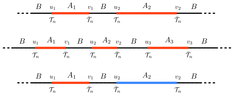
Figure 1: The configurations of intervals considered. Top and middle: the entanglement between a subsystem $A$ made by either two (top) or three (middle) disjoint intervals and the remainder $B$. Bottom: the entanglement between two disjoint intervals $A_{1}$ and $A_{2}$ embedded in a larger system in its ground state made by $A_{1}\cup A_{2}$ and the reminder $B$. In CFT correlation functions of branch-point twist fields $\mathcal{T}_{n}$ and $\bar{\mathcal{T}}_{n}$ placed at the endpoints of the intervals must be computed to get either the entanglement entropy (top and middle panels) or logarithmic negativity (bottom panel) through the proper replica limit.

Taking the limit $n\to 1$ in (1.1) and (1.3) in many interesting cases is highly non trivial. For instance, the analytic continuation of the Rényi entropies of a single interval for the excited states given by the primaries [14, 15] has been studied in [16]. For the excited states given by the descendants a closed expression for all the Rényi entropies is still not known [17]. Interesting features have been observed by considering the Rényi entropies of a single interval in critical one dimensional models for real $n$ but no singularities have been found [18].

In this paper we address the case of disjoint intervals for some models in one spatial dimension. The Rényi entropies for a subsystem $A$ made by $N$ disjoint intervals (see Fig. 1, middle panel for $N=3$) are given by the partition function of the model on a Riemann surface of genus $g=(N-1)(n-1)$. These partition functions can be computed for some simple CFTs like the massless compact boson and the Ising model [7, 8, 19] but finding the corresponding analytic continuations in the most generic case is still beyond our knowledge. For two spatial dimensions, already the simple case of the entanglement entropy of a disk could lead to a difficult replica limit [20].

Another interesting quantity to consider is the logarithmic negativity, which is a measure of entanglement for bipartite mixed states [21]. Let us consider a pure or mixed state characterized by the density matrix $\rho$ acting on a bipartite Hilbert space $\mathcal{H}=\mathcal{H}_{1}\otimes\mathcal{H}_{2}$ and the arbitrary bases $|e_{i}^{(1)}\rangle$ and $|e_{j}^{(2)}\rangle$ for $\mathcal{H}_{1}$ and $\mathcal{H}_{2}$ respectively. The important object to introduce is the partial transpose of $\rho_{A_{1}\cup A_{2}}$ with respect to one of the two parts. Considering e.g. the partial transposition with respect to the second part, the matrix element of $\rho_{A_{1}\cup A_{2}}^{T_{2}}$ is defined as follows

$$\langle e_{i}^{(1)}e_{j}^{(2)}|\rho_{A_{1}\cup A_{2}}^{T_{2}}|e_{k}^{(1)}e_{l}^{(2)}\rangle=\langle e_{i}^{(1)}e_{l}^{(2)}|\rho_{A_{1}\cup A_{2}}|e_{k}^{(1)}e_{j}^{(2)}\rangle\,.$$ (1.5)

Then, the logarithmic negativity is given by

$$\mathcal{E}\equiv\log{\rm Tr}|\rho_{A_{1}\cup A_{2}}^{T_{2}}|\,,$$ (1.6)

where ${\rm Tr}|\rho_{A_{1}\cup A_{2}}^{T_{2}}|$ is the trace norm of the hermitean matrix $\rho_{A_{1}\cup A_{2}}^{T_{2}}$, which is the sum of the absolute values of its eigenvalues. Taking into account the traces ${\rm Tr}(\rho_{A_{1}\cup A_{2}}^{T_{2}})^{n}$ of integer powers of $\rho_{A_{1}\cup A_{2}}^{T_{2}}$, it is not difficult to observe that a parity effect occurs. In particular, considering the sequence of the odd powers $n=n_{o}$ and the one of the even powers $n=n_{e}$, the logarithmic negativity (1.6) can be found through the following replica limit [22, 23]

$$\mathcal{E}=\lim_{n_{e}\to 1}\log{\rm Tr}\big{(}\rho_{A_{1}\cup A_{2}}^{T_{2}}\big{)}^{n_{e}}.$$ (1.7)

Notice that for $n_{o}\to 1$ one simply recovers the normalization condition ${\rm Tr}\rho_{A_{1}\cup A_{2}}^{T_{2}}=1$. For a bipartite pure state a relation occurs between ${\rm Tr}(\rho_{A_{1}\cup A_{2}}^{T_{2}})^{n}$ and the Renyi entropies which tells us that the logarithmic negativity reduces to the Rényi entropy of order $n=1/2$. However, we are interested in the logarithmic negativity of mixed states and the reduced density matrix is an important example. Thus, given a quantum system in a pure state and considering the reduced density matrix $\rho_{A_{1}\cup A_{2}}$ of two adjacent or disjoint spatial regions, while $S_{A_{1}\cup A_{2}}$ measures the entanglement between $A_{1}\cup A_{2}$ and the complementary region $B$, the logarithmic negativity in (1.6) measures the entanglement between $A_{1}$ and $A_{2}$ (see Fig. 1, bottom panel, for one spatial dimension).

In two dimensional CFTs, the logarithmic negativity has been studied in [22, 23] for zero temperature, at finite temperature [24] and also out of equilibrium (the time evolution after a global quench [25] and after a local quench [26] have been considered). For two disjoint intervals at zero temperature ${\rm Tr}(\rho_{A_{1}\cup A_{2}}^{T_{2}})^{n}$ must be computed case by case because it encodes all the CFT data. The replica limit (1.7) for these expressions turns out to be difficult to compute, like for the mutual information. Indeed, analytic results have not been found for all the possible configurations of intervals.

In this paper we numerically extrapolate the entanglement entropy and the logarithmic negativity through their replica limits, which are respectively (1.1) and (1.7), for simple two dimensional CFT models and for configurations of intervals whose analytic continuations for $S_{A}$ and $\mathcal{E}$ are not known. In particular, for the free massless boson, both compactified and in the decompactification regime, and for the Ising model, ${\rm Tr}\rho_{A}^{n}$ are known analytically for a generic number $N$ of disjoint intervals [7, 8, 19], while ${\rm Tr}(\rho_{A_{1}\cup A_{2}}^{T_{2}})^{n}$ is known analytically for two disjoint intervals [22, 23, 27, 28]. We consider some of these models for two or three disjoint intervals (only some configurations in the latter case) and employ a numerical method based on rational interpolations to get the corresponding entanglement entropy or logarithmic negativity. This extrapolating method has been first suggested in this context by [20] (see [29] for other numerical methods). We checked our extrapolations against numerical results found through the corresponding lattice models whenever they are available in the literature, finding very good agreement; otherwise the method provides numerical predictions that could be useful benchmarks for future studies.

The paper is organized as follows. In §2 we extrapolate the mutual information for the compact boson and for the Ising model comparing the results with the corresponding ones found for the XXZ spin chain [6] and the critical Ising chain [9]. In §3 the entanglement entropy of three disjoint intervals is considered for the non compact boson and for the Ising model. While the extrapolations for the former model can be checked against exact results for the periodic harmonic chain, there are no results in the literature about the entanglement entropy of three disjoint intervals for the critical Ising chain to compare with. In §4 we focus on the logarithmic negativity of two disjoint intervals for the non compact boson. The appendix §A contains a discussion about the rational interpolation method that has been employed throughout the paper.

2 Mutual information

In this section, after a quick review of the computation of $I_{A_{1},A_{2}}^{(n)}$ in CFT, we focus on the compactified boson and on the Ising model because $I_{A_{1},A_{2}}^{(n)}$ is known analytically in these cases. The numerical extrapolation of the analytic expressions for $I_{A_{1},A_{2}}^{(n)}$ to $n\to 1$ leads to the mutual information, which can be compared with the corresponding numerical results found from the XXZ spin chain and the Ising chain in a transverse field.

Let us consider a two dimensional CFT with central charge $c$ at zero temperature.
As first discussed in [3], ${\rm Tr}\rho_{A}^{n}$ for a subsystem $A$ made by $N$ disjoint intervals can be computed as the $2N$-point correlation function of branch-point twist fields $\mathcal{T}_{n}$ and $\bar{\mathcal{T}}_{n}$ placed at the endpoints of the intervals in an alternate sequence (see [30] for integrable quantum field theories). These fields have been largely studied in the early days of string theory [31] and their crucial role for the entanglement computations has been exploited during the last decade.

When the subsystem $A$ is a single interval $A=[u,v]$ with length $\ell=|u-v|$ on the infinite line, ${\rm Tr}\rho_{A}^{n}$ is given by the two-point function of branch-point twist fields [3]

$${\rm Tr}\rho_{A}^{n}=\langle\mathcal{T}_{n}(u)\bar{\mathcal{T}}_{n}(v)\rangle=\frac{c_{n}}{|u-v|^{2\Delta_{n}}}\,,\qquad\Delta_{n}=\frac{c}{12}\left(n-\frac{1}{n}\right),$$ (2.1)

where $\Delta_{n}$ are the scaling dimensions of the twist fields $\mathcal{T}_{n}$ and $\bar{\mathcal{T}}_{n}$, being $c_{n}$ a non universal constant such that $c_{1}=1$. Taking the replica limit (1.1) of (2.1) is straightforward and one gets the well known result for the entanglement entropy of an interval in the infinite line [2]

$$S_{A}=\frac{c}{3}\,\log(\ell/a)+c^{\prime}_{1}\,,$$ (2.2)

where $a$ is a UV cutoff. Thus, the entanglement entropy and the Rényi entropies for a single interval depend only on the central charge $c$ of the model.

When the subsystem $A=A_{1}\cup A_{2}$ is made by two disjoint intervals $A_{1}=[u_{1},v_{1}]$ and $A_{2}=[u_{2},v_{2}]$ (with the endpoints ordered as $u_{1}<v_{1}<u_{2}<v_{2}$), the Rényi entropies encode the full data of the CFT because ${\rm Tr}\rho_{A}^{n}$ is obtained as a four-point function of twist fields [7, 8]. By global conformal invariance we have that

$${{\rm Tr}}\rho_{A}^{n} = \langle\mathcal{T}_{n}(u_{1})\bar{\mathcal{T}}_{n}(v_{1})\mathcal{T}_{n}(u_{2})\bar{\mathcal{T}}_{n}(v_{2})\rangle$$ (2.3)

$$= c_{n}^{2}\left[\frac{(u_{2}-u_{1})(v_{2}-v_{1})}{(v_{1}-u_{1})(v_{2}-u_{2})(u_{2}-v_{1})(v_{2}-u_{1})}\right]^{2\Delta_{n}}\mathcal{F}_{2,n}(x)$$ (2.4)

where the four-point ratio reads

$$x=\frac{(u_{1}-v_{1})(u_{2}-v_{2})}{(u_{1}-u_{2})(v_{1}-v_{2})}\,,$$ (2.5)

and $x\in(0,1)$. Since ${{\rm Tr}}\rho_{A}=1$ holds, $\mathcal{F}_{2,1}(x)=1$ identically. The function $\mathcal{F}_{2,n}(x)$ depends on the details of the model and therefore it must be computed case by case. From (2.1) and (2.3), one gets that (1.4) for a CFT is given by

$$I_{A_{1},A_{2}}^{(n)}=-\,\frac{(n+1)c}{6n}\,\log(1-x)+\tilde{I}_{n}(x)\,,\qquad\tilde{I}_{n}(x)\equiv\frac{1}{n-1}\log[\mathcal{F}_{2,n}(x)]\,.$$ (2.6)

Since the mutual information $I_{A_{1},A_{2}}$ is the limit $n\to 1$ of (2.6), as stated in (1.3), it is the function of $x$ given by

$$I_{A_{1},A_{2}}=-\,\frac{c}{3}\,\log(1-x)+\tilde{I}_{1}(x)\,,\qquad\tilde{I}_{1}(x)\equiv\partial_{n}\mathcal{F}_{2,n}(x)\big{|}_{n=1}\,.$$ (2.7)

The explicit expression of $\mathcal{F}_{2,n}(x)$ is known for some simple models like the free compact boson and the Ising model. In these cases $\mathcal{F}_{2,n}(x)$ is written in terms of the Riemann theta function, which is defined as follows [32]

$$\Theta[\boldsymbol{e}](\boldsymbol{z}|\Omega)\equiv\sum_{\boldsymbol{m}\;\in\;\mathbb{Z}^{p}}\exp\left[\,\textrm{i}(\boldsymbol{m}+\boldsymbol{\varepsilon})^{\textrm{t}}\cdot\Omega\cdot(\boldsymbol{m}+\boldsymbol{\varepsilon})+2\pi\textrm{i}(\boldsymbol{m}+\boldsymbol{\varepsilon})^{\textrm{t}}\cdot(\boldsymbol{z}+\boldsymbol{\delta})\right]\,,$$ (2.8)

where $\Omega$ is a $p\times p$ symmetric complex matrix with positive immaginary part and $\boldsymbol{z}\in\mathbb{C}^{p}/(\mathbb{Z}^{p}+\Omega\mathbb{Z}^{p})$ is a complex $p$ dimensional vector. The vector $\boldsymbol{e}^{\textrm{t}}\equiv(\boldsymbol{\varepsilon^{\textrm{t}}},\boldsymbol{\delta}^{\textrm{t}})$ is the characteristic of the Riemann theta function (2.8), being $\boldsymbol{\varepsilon}$ and $\boldsymbol{\delta}$ two $p$ dimensional vectors whose elements are either $0$ or $1/2$. The characteristic provides the parity of (2.8) as function of $\boldsymbol{z}$, which is the same one of the integer number $4\boldsymbol{\varepsilon}^{\textrm{t}}\cdot\boldsymbol{\delta}$, indeed

$$\Theta[\boldsymbol{e}](-\boldsymbol{z}|\Omega)=(-1)^{4\boldsymbol{\varepsilon}\cdot\boldsymbol{\delta}}\,\Theta[\boldsymbol{e}](\boldsymbol{z}|\Omega)\,.$$ (2.9)

It is not difficult to realize that there are $2^{p-1}(2^{p}+1)$ even characteristics and $2^{p-1}(2^{p}-1)$ odd ones. Since in this paper we always deal with $\boldsymbol{z}=\boldsymbol{0}$, we find it convenient to lighten the formulas by introducing the notation $\Theta[\boldsymbol{e}](\Omega)\equiv\Theta[\boldsymbol{e}](\boldsymbol{0}|\Omega)$ and $\Theta(\Omega)\equiv\Theta[\boldsymbol{0}](\Omega)$. The Riemann theta functions throughout this paper have been evaluated by using Mathematica through the built-in function SiegelTheta.

As a first example, we consider the free boson compactified on a circle of radius $r$, which has $c=1$. The corresponding $\mathcal{F}_{2,n}(x)$ for any integer $n\geqslant 2$ is given by [7]

$$\mathcal{F}_{2,n}(x)=\frac{\Theta(\eta\tau_{2})\,\Theta(\tau_{2}/\eta)}{\Theta(\tau_{2})^{2}}\,,$$ (2.10)

where $\eta\propto r^{2}$ and $\tau_{2}=\tau_{2}(x)$ is the $(n-1)\times(n-1)$ purely imaginary period matrix of the Riemann surface which underlies the computation of ${{\rm Tr}}\rho_{A}^{n}$, whose elements read

$$(\tau_{2})_{ij}\,\equiv\,\textrm{i}\,\frac{2}{n}\sum_{k=1}^{n-1}\sin(\pi k/n)\,\frac{F_{k/n}(1-x)}{F_{k/n}(x)}\,\cos[2\pi(i-j)k/n]\,,$$ (2.11)

where $F_{s}(x)\equiv\,_{2}F_{1}(s,1-s;1;x)$, being ${}_{2}F_{1}$ the hypergeometric function. Notice that $\mathcal{F}_{2,n}(0)=1$. Moreover, $\mathcal{F}_{2,n}(x)$ is invariant under $\eta\rightarrow 1/\eta$ and $x\rightarrow 1-x$ separately. The latter symmetry is related to the well known property $S_{A}=S_{B}$ of the entanglement entropy for pure states in the case of $A$ made by two disjoint intervals. It is worth remarking that (2.10) holds for $x\in(0,1)$. Indeed, when $x\in\mathbb{C}$ and $x\notin(0,1)$ the corresponding expression is slightly more complicated [23] and it enters in the computation of the logarithmic negativity for the compact boson.

In order to find the analytic expression of the mutual information for the compact boson, one has to compute $\tilde{I}_{1}(x)$ in (2.7) with $\mathcal{F}_{2,n}(x)$ given by (2.10). Since performing this analytic computation is still an open problem, we employ the numerical extrapolation method suggested by [20] (see §A) to get a result that can be compared with the numerical data found in [6] from the XXZ spin chain.

Before entering in the numerical analysis, it is worth discussing the decompactification regime, which can be addressed analytically. The non compact boson corresponds to the regime $\eta\gg 1$ (or $\eta\ll 1$ because of the symmetry $\eta\leftrightarrow 1/\eta$) in the above expressions. In [7] it has been found that, for $\eta\ll 1$, the terms $\tilde{I}_{1}(x)$ in (2.7) becomes

$$\tilde{I}_{1}(x)\big{|}_{\eta\ll 1}=-\frac{1}{2}\log\eta+\frac{D(x)+D(1-x)}{2}\,,\qquad D(x)\equiv-\int_{-\textrm{i}\infty}^{\textrm{i}\infty}\frac{dz}{\textrm{i}}\,\frac{\pi z}{\sin(\pi z)}\log[F_{z}(x)]\,.$$ (2.12)

The Hamiltonian of the periodic XXZ spin $1/2$ chain in a magnetic field $h$ reads [33]

$$H_{\textrm{\tiny XXZ}}\equiv\sum_{j=1}^{L}\big{(}S^{x}_{j}S^{x}_{j+1}+S^{y}_{j}S^{y}_{j+1}+\Delta\,S^{z}_{j}S^{z}_{j+1}\big{)}-h\sum_{j=1}^{L}S^{z}_{j}\,,$$ (2.13)

where $S^{a}_{j}=\sigma^{a}_{j}/2$, being $\sigma^{a}_{j}$ the standard Pauli matrices acting on the spin at the $j$-th site. The chain has $L$ sites and $\Delta$ is the anisotropy. The mutual information for this lattice model has been computed in [6] by direct diagonalization for $L\leqslant 30$. When $h=0$ and $-1<\Delta\leqslant 1$ the model in the continuum is described by the $c=1$ compact boson with $\eta=1-(1/\pi)\arccos\Delta$, while for $h\neq 0$ an explicit formula providing $\eta$ does not exist and therefore it must be found numerically. The CFT formulas reviewed above can be applied also to the case of a finite system of length $L$ with periodic boundary conditions by employing a conformal mapping from the cylinder to the plane. As final result, the CFT formulas for this case are obtained by considering the expressions for the infinite line and replacing any length $\ell_{i}$ with the corresponding chord length $(L/\pi)\sin(\pi\ell_{i}/L)$ [3].

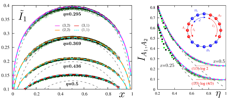
Figure 2: Mutual information for the XXZ model. The data points are extracted from [6] and the coloured curves are obtained from the rational interpolations of the analytic expressions (2.6) and (2.10) for the compact boson with the values of $(p,q)$ indicated in the left panel. The dashed grey lines correspond to the decompactification regime, where the analytic continuation (2.12) is known. Left: $\tilde{I}_{1}$, defined in (2.7), as function of $x$ for various values of $\eta$. Right: the mutual information $I_{A_{1},A_{2}}$ as function of $\eta$ for two fixed values of $x$.

Let us consider the mutual information of the compactified boson as first example of our extrapolation method. For any fixed value of $x$, we have that $I_{A_{1},A_{2}}^{(n)}$ are given analytically by (2.6) and (2.10) for any positive integer $n\geqslant 2$, while the corresponding analytic continuation to $n=1$ is estimated by performing a numerical extrapolation of the known data through a rational function. The latter one is characterized by two positive integer parameters $p$ and $q$, which are the degrees of the numerator and of the denominator respectively. As explained in §A, to perform a rational interpolation characterized by the pair $(p,q)$ we need at least $p+q+1$ known data. An important technical difficulty that one encounters is the evaluation of the Riemann theta functions for large genus period matrices, i.e. for high values of $n$. Given the computational resources at our disposal, we were able to compute Riemann theta functions containing matrices whose size is at most $12$. For the compactified boson this corresponds to $n_{\text{max}}=11$ and therefore $p+q+1\leqslant 10$.

In Fig. 2 we compared our numerical extrapolations of the analytic expressions of [7] with the numerical data for the XXZ spin chain computed in [6] by exact diagonalization, finding a very good agreement. In the left panel $\tilde{I}_{1}$ is shown as function of the four-point ratio $x$ for different values of the parameter $\eta$, while in the right panel the mutual information $I_{A_{1},A_{2}}$ is shown as function of $\eta$ for the two fixed configurations of intervals given by $\ell_{1}=\ell_{2}=d_{1}=d_{2}=L/4$ ($x=0.5$) and $2\ell_{1}=2\ell_{2}=d_{1}=d_{2}=L/3$ ($x=0.25$), being $L$ the total length of the periodic system. All the rational interpolations in the figure exhibit a good agreement with the numerical data, despite the low values of $p$ and $q$. Increasing these parameters, a better approximation is expected but the result is already stable for these values and we provided two rational interpolations for each curve as a check. Some rational interpolations may display some spurious bahaviour in some regimes of $x$. As discussed in detail in §A, this possibility increases with $q$. These results have been discarded and we showed only rational interpolations which are well-behaved in the whole domain $x\in(0,1)$. Notice that rational interpolations that are well-behaved for some $\eta$ and $x$ could display some bad behaviour changing them. Thus, the values of $(p,q)$ must be chosen case by case. In Fig. 2 the dashed grey lines are obtained from the analytic continuation (2.12) found in [7], which corresponds to the decompactification regime and therefore it reproduces the numerical data from the XXZ chain and from the rational interpolations only for small $\eta$, as expected.

Another important case where the Rényi entropies of two disjoint intervals have been found analytically is the Ising model [8]. The Hamiltonian of the one dimensional spin chain defining the Ising model in a transverse field is

$$H_{\textrm{\tiny Ising}}\equiv-\sum_{j=1}^{L}\big{(}\sigma^{x}_{j}\sigma^{x}_{j+1}+h\,\sigma^{z}_{j}\big{)}\,,$$ (2.14)

where periodic boundary conditions are imposed. This model has a quantum critical point at $h=1$ and in the continuum it is a free Majorana fermion with central charge $c=1/2$. The Rényi entropies for two disjoint intervals on the spin chain (2.14) have been studied in [9] through a Tree Tensor Network algorithm [34] and in [10] through the exact solution of the model in terms of free Majorana fermions. The former method allowed to find also the mutual information.

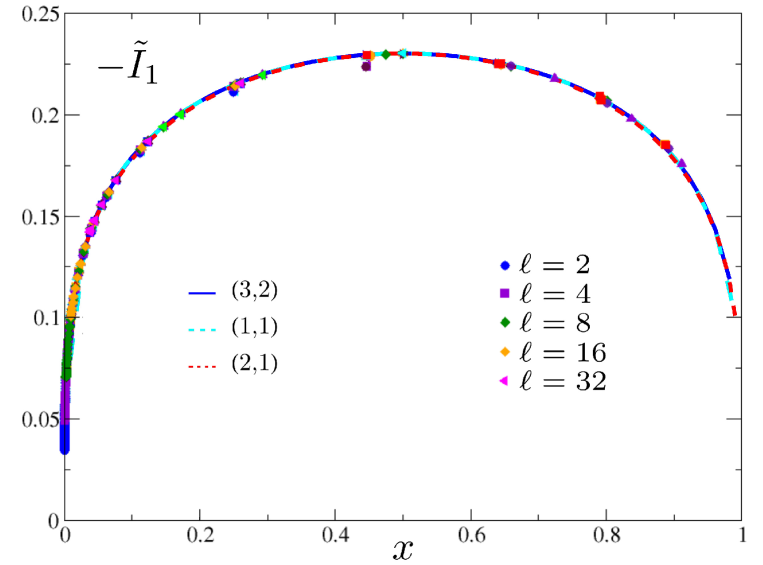
Figure 3: Extrapolations for $-\tilde{I}_{1}$, defined in (2.7), as function of $x$ for the Ising model. The data points are extracted from [9] while the coloured curves are obtained through the rational interpolations with $(p,q)$ indicated.

As for the Rényi entropies for two disjoint intervals in corresponding CFT, by employing known results about bosonization on higher genus Riemann surfaces for $c=1$ models [31], the expression of $\mathcal{F}_{2,n}(x)$ for the Ising model can be written in terms of Riemann theta functions (2.8) evaluated for the period matrix $\tau_{2}$ in (2.11). In particular, ${\rm Tr}\rho_{A_{1}\cup A_{2}}^{n}$ for the Ising model is given by (2.4) with $c=1/2$ and [8]

$$\mathcal{F}_{2,n}(x)=\frac{\sum_{\boldsymbol{e}}\left|\Theta[\boldsymbol{e}](\tau_{2})\right|}{2^{n-1}\left|\Theta(\tau_{2})\right|}\,,$$ (2.15)

where the sum is performed over all the possible characteristics $\boldsymbol{e}^{\textrm{t}}\equiv(\boldsymbol{\varepsilon^{\textrm{t}}},\boldsymbol{\delta}^{\textrm{t}})$, being $\boldsymbol{\varepsilon}$ and $\boldsymbol{\delta}$ two $n-1$ dimensional vectors whose elements are either $0$ or $1/2$. Let us remark that in the sum (2.15) only the $2^{n-2}(2^{n-1}+1)$ even characteristics occur. Thus, the mutual information for the Ising model is (2.7) with $\mathcal{F}_{2,n}(x)$ given by (2.15). Similarly to the case of the compact boson, also for the Ising model we are not able to compute $\tilde{I}_{1}(x)$ analytically and therefore we perform a numerical extrapolation through the rational interpolation method described in §A.

In Fig. 3 we show $-\tilde{I}_{1}(x)$ as function of $x\in(0,1)$, which can be found by considering two disjoint intervals of equal length, and compare the numerical data obtained in [9] with the curve found through the numerical extrapolation of the corresponding formula containing (2.15) through rational interpolations. Since (2.15) contains Riemann theta functions, we cannot consider high values for $n$, like for the compact boson. Moreover, in this case one faces an additional complication with respect to the compact boson because in (2.15) the sum over all the even characteristics occurs and the number of terms in the sum grows exponentially with $n$. Given our computational power, we have computed the Rényi entropies up to $n=7$ and in Fig. 3 we show the rational interpolations found by choosing three different pairs $(p,q)$ which are well-behaved among the available ones. Since the curves coincide, the final result is quite stable and, moreover, the agreement with the numerical data found in [9] through the Tree Tensor Network is very good.

3 Three disjoint intervals

In this section we partially extend the analysis done in §2 by considering the case of three disjoint intervals. After a brief review of the analytic results known for a generic number $N$ of disjoint intervals, we focus on $N=3$ and perform some numerical extrapolations for the non compact boson and for the Ising model.

Given a the spatial subsystem $A=\cup_{i=1}^{N}A_{i}$ made by the union of the $N$ disjoint intervals $A_{1}=[u_{1},v_{1}]$, $\dots$, $A_{N}=[u_{N},v_{N}]$, a generalization of (1.4) to $N\geqslant 2$ reads [19]

$$I^{(n)}_{A_{1},\cdots,A_{N}}\equiv\frac{(-1)^{N}}{n-1}\log R_{N,n}\,,\qquad R_{N,n}\equiv\prod_{p=1}^{N}\prod_{\sigma_{N,p}}\left({\rm Tr}\rho^{n}_{\sigma_{N,p}}\right)^{(-1)^{N-p}}\,,$$ (3.1)

where $\sigma_{N,p}$ denotes the union of a generic choice of $1\leqslant p\leqslant N$ intervals among the $N$ ones. It is straightforward to observe that the analytic continuation $n\to 1$ of (3.1), i.e.

$$I_{A_{1},\dots,A_{N}}\equiv\lim_{n\rightarrow 1}I_{A_{1},\dots,A_{N}}^{(n)}\,,$$ (3.2)

provides a natural generalization to $N\geqslant 2$ of the mutual information (1.3). We find it useful to normalise the quantities introduced in (3.1) and (3.2) by themselves evaluated for some fixed configuration of intervals, namely

$$R^{\textrm{\tiny{norm}}}_{N,n}\equiv\frac{R_{N,n}}{R_{N,n}\big{|}_{\textrm{\tiny{fixed}}}}\,,\qquad I^{\textrm{\tiny{sub}}}_{N}\equiv I_{N}-I_{N}\big{|}_{\textrm{\tiny{fixed}}}=\lim_{n\to 1}R^{\textrm{\tiny{norm}}}_{N,n}\,,$$ (3.3)

where we have adopted the shorthand notation $I_{N}\equiv I_{A_{1},\dots,A_{N}}$.

In two dimensional CFTs, the expression of ${\rm Tr}\rho_{A}^{n}$ for $N$ disjoint intervals can be written as a $2N$-point function of twist fields [3, 4]. Similarly to the two intervals case, the global conformal invariance cannot fix the dependence on $u_{i}$ and $v_{i}$. In particular, given the endpoints $u_{1}<v_{1}<\dots<u_{N}<v_{N}$, one can employ the following conformal map

$$w_{N}(z)=\frac{(u_{1}-z)(u_{N}-v_{N})}{(u_{1}-u_{N})(z-v_{N})}\,,$$ (3.4)

which sends $u_{1}\rightarrow 0$, $u_{N}\rightarrow 1$ and $v_{N}\rightarrow\infty$. The remaining endpoints are mapped into the $2N-3$ four-point ratios $x_{1}=w_{N}(v_{1}),\,x_{2}=w_{N}(u_{2}),\,x_{3}=w_{N}(v_{2}),\dots,x_{2N-3}=w_{N}(v_{N-1})$ which are invariant under $SL(2,\mathbb{C})$. Notice that $x_{j}\in\mathbb{R}$ and the order is preserved, namely $0<x_{1}<x_{2}<\dots<x_{2N-3}<1$.

The global conformal invariance allows us to write ${\rm Tr}\rho_{A}^{n}$ for $N$ disjoint intervals as follows [4]

$${\rm Tr}\rho_{A}^{n}=\langle\prod_{i=1}^{N}\mathcal{T}_{n}(u_{i})\mathcal{\bar{T}}_{n}(v_{i})\rangle=c_{n}^{N}\left|\frac{\prod_{i<j}(u_{j}-u_{i})(v_{j}-v_{i})}{\prod_{i,j}(v_{j}-u_{i})}\right|^{2\Delta_{n}}\mathcal{F}_{N,n}(\boldsymbol{x})\,,$$ (3.5)

where $i,j=1,\dots,N$, the scaling dimension $\Delta_{n}$ is given in (2.1) and $\boldsymbol{x}$ is the vector whose elements are the $2N-3$ four-point ratios introduced above. It is worth remarking that $\mathcal{F}_{N,n}(\boldsymbol{x})$ encodes the full operator content of the model and therefore its computation depends on the features of the model. From (3.1) and (3.5), one finds that $R_{N,n}$ and $R^{\textrm{\tiny{norm}}}_{N,n}$ in CFT become respectively [19]

$$R_{N,n}(\boldsymbol{x})=\prod_{p\,=\,2}^{N}\,\prod_{\sigma_{N,p}}\big{[}\mathcal{F}_{p,n}(\boldsymbol{x}^{\sigma_{N,p}})\big{]}^{(-1)^{N-p}}\,,\qquad R^{\textrm{\tiny{norm}}}_{N,n}(\boldsymbol{x})=\frac{R_{N,n}(\boldsymbol{x})}{R_{N,n}(\boldsymbol{x}_{\textrm{\tiny{fixed}}})}\,,$$ (3.6)

where $\boldsymbol{x}^{\sigma_{N,p}}$ is the vector made by the $2p-3$ four-point ratios obtained with the endpoints of the $p$ intervals selected by $\sigma_{N,p}$.

The function $\mathcal{F}_{N,n}(\boldsymbol{x})$ for the compactified boson has been studied in [19] by generalizing the construction of [7] and, again, it is written in terms of the Riemann theta function (2.8). For $N>2$ disjoint intervals the Riemann surface occurring in the computation of ${\rm Tr}\rho_{A}^{n}$ has genus $g=(N-1)(n-1)$. The corresponding $g\times g$ period matrix $\tau_{N}=\mathcal{R}+\textrm{i}\,\mathcal{I}$, which is symmetric and complex with positive imaginary part, is complicated and, since we do not find instructive to report it here, we refer to [19] for any detail about it. The expression of $\mathcal{F}_{N,n}(\boldsymbol{x})$ for the compactified boson reads [31, 19]

$$\mathcal{F}_{N,n}(\boldsymbol{x})=\frac{\Theta(T_{\eta})}{|\Theta(\tau_{N})|^{2}}\,,\qquad T_{\eta}\equiv\begin{pmatrix}\,\textrm{i}\,\eta\,\mathcal{I}&\mathcal{R}\\ \mathcal{R}&\textrm{i}\,\mathcal{I}/\eta\,\\ \end{pmatrix},$$ (3.7)

where $\eta$ is the parameter containing the compactification radius introduced in §2. Notice that (3.7) is invariant under $\eta\leftrightarrow 1/\eta$.

As done in §2 for the two intervals case, also for $N$ disjoint intervals it is interesting to consider the decompactification regime. When $\eta\gg 1$ the expression in (3.7) becomes

$$\mathcal{F}_{N,n}^{\eta\rightarrow\infty}(\boldsymbol{x})=\frac{\eta^{g/2}}{\sqrt{\textrm{det}(\mathcal{I})}\,|\Theta(\tau_{N})|^{2}}\equiv\eta^{g/2}\,\widehat{\mathcal{F}}_{N,n}(\boldsymbol{x})\,.$$ (3.8)

For computational purposes, it is important to observe that in (3.8) the Riemann theta function is evaluated for $\tau_{N}$, which is $g\times g$, while for finite $\eta$, when (3.7) holds, the matrix occurring in the Riemann theta function is $2g\times 2g$. This implies that for the non compact boson we can reach higher values of $n$ and therefore the corresponding numerical extrapolation is more precise. In the decompactification regime we can also appreciate the convenience of considering the normalization (3.3). Indeed, plugging (3.8) into (3.6) one obtains an expression which is $\eta$ independent

$$\widehat{R}^{\textrm{\tiny{norm}}}_{N,n}(\boldsymbol{x})\equiv\frac{R_{N,n}^{\eta\rightarrow\infty}(\boldsymbol{x})}{R_{N,n}^{\eta\rightarrow\infty}(\boldsymbol{x}_{\textrm{\tiny{fixed}}})}=\prod_{p\,=\,2}^{N}\,\prod_{\sigma_{N,p}}\left[\frac{\widehat{\mathcal{F}}_{p,n}(\boldsymbol{x}^{\sigma_{N,p}})}{\widehat{\mathcal{F}}_{p,n}(\boldsymbol{x}^{\sigma_{N,p}}_{\textrm{\tiny{fixed}}})}\right]^{(-1)^{N-p}}.$$ (3.9)

As for the Ising model, since the results of [31] about the bosonization on higher genus Riemann surfaces for $c=1$ models hold for a generic genus, we can straightforwardly write the generalization to $N\geqslant 2$ of the $N=2$ formula (2.15). Indeed, given the period matrix $\tau_{N}$ employed for the compact boson in (3.7), we have that ${\rm Tr}\rho_{A}^{n}$ for the Ising model is (3.5) with $c=1/2$ and [31, 19]

$$\mathcal{F}_{N,n}(\boldsymbol{x})=\frac{\sum_{\boldsymbol{e}}|\Theta[\boldsymbol{e}](\tau_{N})|}{2^{g}\,|\Theta(\tau_{N})|}\,.$$ (3.10)

The Riemann theta functions in this formula are evaluated for the $g\times g$ period matrix and a sum over all the characteristics occurs. It is worth remarking that the Riemann theta functions in (3.10) with odd characteristics vanish and therefore the sum contains $2^{g-1}(2^{g}+1)$ terms. In [19] the formula (3.10) has been checked numerically on the lattice for $n=2$, various $N$ and different configurations of intervals by employing the Matrix Product States. To our knowledge, numerical results for $I_{N}$ with $N\geqslant 3$ are not available in the literature for the critical Ising chain in transverse field.

In this paper, for simplicity, we consider only $N=3$ disjoint intervals and therefore let us specify some of the formulas given above to this case. The generalization of the mutual information to the case of three disjoint intervals is given by

$$I_{A_{1},A_{2},A_{3}}\equiv S_{A_{1}}+S_{A_{2}}+S_{A_{3}}-S_{A_{1}\cup A_{2}}-S_{A_{1}\cup A_{3}}-S_{A_{2}\cup A_{3}}+S_{A_{1}\cup A_{2}\cup A_{3}}=\lim_{n\to 1}I^{(n)}_{A_{1},A_{2},A_{3}}\,,$$ (3.11)

where $I^{(n)}_{A_{1},A_{2},A_{3}}$ can be written by specifying the expressions in (3.1) to $N=3$, namely

$$I^{(n)}_{A_{1},A_{2},A_{3}}\equiv\,\frac{\log(R_{3,n})}{1-n}\,=\,S^{(n)}_{A_{1}}+S^{(n)}_{A_{2}}+S^{(n)}_{A_{3}}-S^{(n)}_{A_{1}\cup A_{2}}-S^{(n)}_{A_{1}\cup A_{3}}-S^{(n)}_{A_{2}\cup A_{3}}+S^{(n)}_{A_{1}\cup A_{2}\cup A_{3}}\,,$$ (3.12)

with

$$R_{3,n}\equiv\frac{{\rm Tr}\rho^{n}_{A_{1}\cup A_{2}\cup A_{3}}\big{(}{\rm Tr}\rho^{n}_{A_{1}}{\rm Tr}\rho^{n}_{A_{2}}{\rm Tr}\rho^{n}_{A_{3}}\big{)}}{{\rm Tr}\rho^{n}_{A_{1}\cup A_{2}}{\rm Tr}\rho^{n}_{A_{1}\cup A_{3}}{\rm Tr}\rho^{n}_{A_{2}\cup A_{3}}}\,.$$ (3.13)

Considering CFTs, when $N=3$ the vector $\boldsymbol{x}=(x_{1},x_{2},x_{3})$ is made by three four-point ratios and (3.6) becomes

$$R_{3,n}(\boldsymbol{x})=\frac{\mathcal{F}_{3,n}(x_{1},x_{2},x_{3})}{\mathcal{F}_{2,n}(\frac{x_{1}(x_{3}-x_{2})}{x_{2}(x_{3}-x_{1})})\,\mathcal{F}_{2,n}(x_{1})\,\mathcal{F}_{2,n}(\frac{x_{3}-x_{2}}{1-x_{2}})}\,,$$ (3.14)

where $\mathcal{F}_{3,n}(\boldsymbol{x})$ is (3.5) for $N=3$ and $\mathcal{F}_{2,n}(x)$ has been introduced in (2.4).

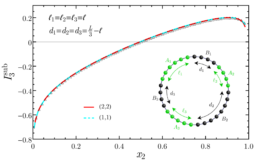
Figure 4: Extrapolations of $I^{\textrm{\tiny{sub}}}_{3}$ (see (3.3) with $N=3$) as function of the four-point ratio $x_{2}$ for the non compact boson. The points are the data obtained in [19] from the periodic harmonic chain (3.15) with $L=5000$ and $\omega L=10^{-5}$. The configuration chosen here is made by equal intervals separated by equal distances, while the fixed configuration normalizing $I^{\textrm{\tiny{sub}}}_{3}$ is given in the text. The coloured lines correspond to two different extrapolations obtained through rational interpolations with $(p,q)$ indicated.

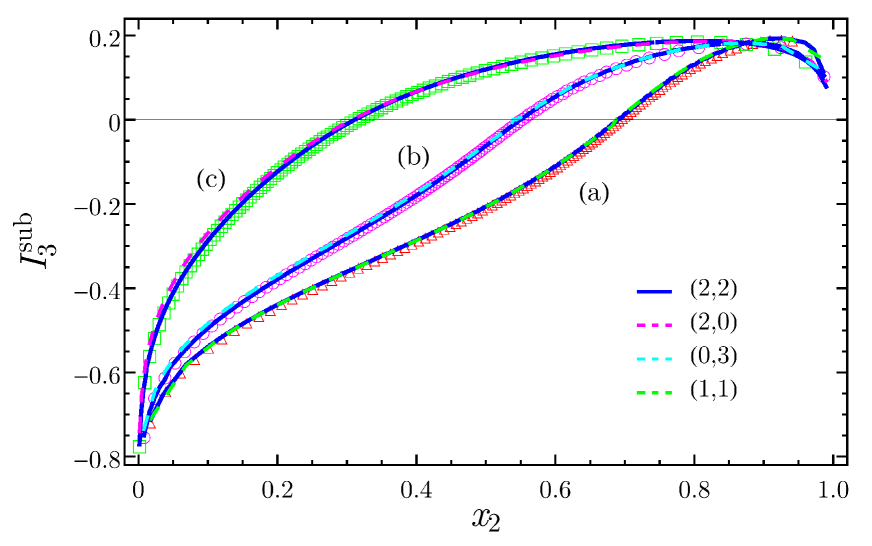
Figure 5: Extrapolations of $I^{\textrm{\tiny{sub}}}_{3}$ for the non compact boson. The harmonic chain is the same one of Fig. 4 while the configurations of intervals are given by (3.16). The data for the periodic harmonic chain have been extracted from [19].

The non compact boson is the CFT describing the massless harmonic chain in the continuum. The Hamiltonian of the harmonic chain with $L$ lattice sites and with nearest neighbour interaction reads

$$H=\sum_{n=0}^{L-1}\left(\frac{1}{2M}\,p_{n}^{2}+\frac{M\omega^{2}}{2}\,q_{n}^{2}+\frac{K}{2}(q_{n+1}-q_{n})^{2}\right),$$ (3.15)

where periodic boundary conditions are imposed. Rewriting (3.15) in terms of $a\equiv\sqrt{M/K}$ and $\omega$ through a canonical transformation, one can observe that it provides the lattice discretization of the free boson with mass $\omega$ and lattice spacing $a$. Thus, the continuum limit of the $\omega=0$ case is the decompactified boson discussed above. The method to compute Rényi entropies for the lattice model (3.15) is well known [35] and ${\rm Tr}\rho_{A}^{n}$ can be found from the correlators $\langle q_{r}q_{s}\rangle$ and $\langle p_{r}p_{s}\rangle$. Let us recall that setting $\omega$ to zero leads to a divergent expression for $\langle q_{r}q_{s}\rangle$ because of the zero mode occurring for periodic boundary conditions. In [19] the method discussed in [35] has been applied to perform various checks of the CFT formulas for the non compact boson at fixed $n$. Moreover, also $I^{\textrm{\tiny{sub}}}_{N}$ has been found from the harmonic chain data, but a comparison with the analytic results has not been done because the analytic continuation of the corresponding Rényi entropies is not known yet. Indeed, the Riemann theta function occurs in (3.8) and its analytic continuation in $n$ is still an open problem. As for the values of $\omega$, in [19] it has been checked that $\omega L=10^{-5}$ is small enough to capture the CFT regime through the periodic harmonic chain. The numerical data for the periodic harmonic chain have been found by setting $M=K=1$ and $\omega L=10^{-5}$ in (3.15). The same quantities evaluated for $\omega L=10^{-3}$ turned out to be indistinguishable.

In the remaining part of this section we focus on the case of three disjoint intervals and perform some numerical extrapolations of the analytic results reviewed above to $n=1$ through rational interpolations, comparing them with the corresponding numerical data from the lattice models, whenever they are available.

In Figs. 4 and 5 we consider $I^{\textrm{\tiny{sub}}}_{3}$ (see (3.3)) for the decompactified boson, comparing the results obtained for the periodic harmonic chain with the numerical extrapolations found for the corresponding configurations of intervals obtained through the rational interpolation (see §A). The dots are numerical data obtained in [19] from the periodic harmonic chain given by (3.15) with $L=5000$ and different sets of data correspond to different configurations of the three intervals. In particular, referring to the inset of Fig. 4 for the notation, the configuration considered in Fig. 4 is the one where all intervals are equal $\ell_{1}=\ell_{2}=\ell_{3}$ and they are placed at the same distance $d_{1}=d_{2}=d_{3}=L/3-\ell$. Varying the length $\ell$ of the intervals, one finds the result, which is plotted as function of the four-point ratio $x_{2}$. In Fig. 5, the data are labeled according to the following configurations of the three intervals:

$$\begin{array}[]{ccl}\textrm{(a)}&&\textrm{$\ell_{i}=\lambda_{i}\ell$, $d_{i}=(L-\sum_{i=1}^{3}\ell_{i})/3$ with $\lambda_{1}=1$, $\lambda_{2}=2$, $\lambda_{3}=8$;}\\ \textrm{(b)}&&\textrm{\phantom{$\ell_{i}=\lambda_{i}\ell$, $d_{i}=(L-\sum_{i=1}^{3}\ell_{i})/3$} with $\lambda_{1}=1$, $\lambda_{2}=11$, $\lambda_{3}=11$;}\\ \textrm{(c)}&&\textrm{$\ell_{i}=\gamma_{i}\ell$, $d_{i}=\gamma_{i}d$, $d=L/(\sum_{i=1}^{3}\gamma_{i})-\ell$ with $\gamma_{1}=1$, $\gamma_{2}=3$, $\gamma_{3}=6$;}\end{array}$$ (3.16)

where the parameter $\ell$ is varied and the results are plotted as functions of $x_{2}\in(0,1)$. As for the fixed configuration normalizing $I^{\textrm{\tiny{sub}}}_{3}$ in (3.3) we have chosen $\ell_{1}=\ell_{2}=\ell_{3}=d_{1}=d_{2}=\textrm{int}(L/6)$, where $\textrm{int}(\dots)$ denotes the integer part. The coloured curves in Figs. 4 and 5 are the numerical extrapolations of the CFT formulas for the non compact boson (3.8) and (3.9) through the rational interpolation method. For each set of data, we show two different rational interpolations which are well-behaved in order to check the stability of the result. The differences between different well-behaved rational interpolations are very small and the agreement with the numerical data from the harmonic chain is very good, supporting the validity of the extrapolating method. In Figs. 4 and 5 we have employed $2\leqslant n\leqslant 6$. It is worth remarking at this point that the Riemann theta functions occurring in the CFT expression (3.14) for the non compact boson contain at most $g\times g$ matrices ($g=2(n-1)$ for $N=3$) while for the compact boson their size is at most $2g\times 2g$ (see (3.7)). From the computational viewpoint, this is an important difference because the higher is $n$ that can be addressed, the higher is the number of different $(p,q)$ that can be considered in the rational interpolations. Thus, the maximum $n$ that we can deal with is related to the maximum size of the matrices in the Riemann theta functions occurring in the model. Nevertheless, from Figs. 4 and 5 we observe that, for this case, rational interpolations with low values of $(p,q)$ are enough to capture the result expected from the lattice data.

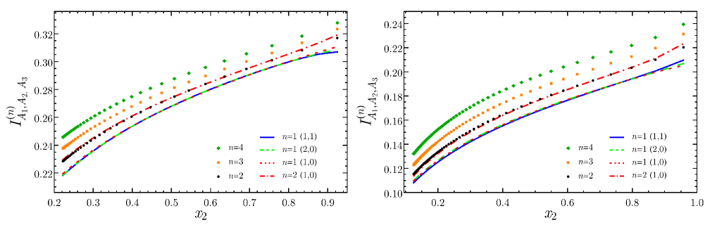
Figure 6: Extrapolations of $I_{A_{1},A_{2},A_{3}}$, defined in (3.11), for the Ising model. Two configurations of intervals have been considered, namely (3.17) with $\alpha=0.25$ (left) and $\alpha=2$ (right). The dots correspond to $I^{(n)}_{A_{1},A_{2},A_{3}}$ in (3.12) with $n\in\{2,3,4\}$ while the lines are the extrapolations obtained through the rational interpolation method with the values of $(p,q)$ indicated. The dot-dashed line is the extrapolation to $n=2$ performed as a check of the method, while the remaining lines correspond to $I_{A_{1},A_{2},A_{3}}$.

In Fig. 6 we show $I_{A_{1},A_{2},A_{3}}$, defined in (3.11), for the Ising model. We have considered the following configurations of three intervals specified by a parameter $\alpha$ (see the inset of Fig. 4 for the notation)

$$\begin{array}[]{ccl}\textrm{(d)}&&\textrm{$\ell_{i}=\ell$, $d_{1}=d_{2}=\alpha\ell$, $d_{3}=L-(3+2\alpha)\ell$\,.}\end{array}$$ (3.17)

In particular, the results in Fig. 6 correspond to $\alpha=0.25$ (left panel) and $\alpha=2$ (right panel), where the dots denote the values of $I^{(n)}_{A_{1},A_{2},A_{3}}$ for $n\in\{2,3,4\}$. Unfortunately, with the computational resources at our disposal, we could not compute Rényi entropies for higher values of $n$. Indeed, besides the problem of computing the Riemann theta function numerically for large period matrices, the additional obstacle occurring for the Ising model is that the number of elements in the sum (3.10) grows exponentially with $n$. Given the few $n$’s available, only few rational interpolations can be employed to approximate the analytic continuation to $n=1$ and they are depicted in Fig. 6 through solid and dashed lines (in general we never use $(p,q)=(0,1)$ because is often not well-behaved). It is interesting to observe that the three different rational interpolations provide the same extrapolation to $n=1$ for a large range of $x_{2}$ (they differ when $x_{2}$ is close to 1). Since, to our knowledge, numerical results about $I_{A_{1},A_{2},A_{3}}$ for the Ising model are not available in the literature, the curves in Fig. 6 are predictions that would be interesting to test through other methods.
In order to check the reliability of the numerical method, we have performed rational interpolations considering only $n\in\{3,4\}$ to extrapolate the value at $n=2$, which is known analytically. Since only two points are available, only the rational interpolation with $(p,q)=(1,0)$ can be done, which is given by the dot-dashed curve in Fig. 6. Despite the roughness of the extrapolation due to the few input points, the agreement with the expected values computed with the analytic expression (black dots) is very good.

4 Entanglement negativity of two disjoint intervals

In this section we consider the logarithmic negativity of two disjoint intervals for the non compact massless free boson, whose analytic formula is not known.

The method to compute the logarithmic negativity $\mathcal{E}$ in quantum field theory and in conformal field theory has been described in [22, 23] (see [24] for the finite temperature case) and we refer to these papers for all the details and the discussion of further cases. In order to briefly mention the main idea, let us consider a subsystem $A=\cup_{i=1}^{N}A_{i}$ made by $N$ disjoint intervals $A_{i}=[u_{i},v_{i}]$. The traces ${\rm Tr}\rho_{A}^{n}$ in CFT are given by the correlators of twist fields in (3.5). Denoting by $A_{0}\varsubsetneq A$ a set of $N_{0}<N$ disjoint intervals among the ones in $A$ and by $\rho_{A}^{T_{0}}$ the partial transpose of $\rho_{A}$ with respect to $A_{0}$, we have that ${\rm Tr}(\rho_{A}^{T_{0}})^{n}$ in CFT is the correlation function of twist fields obtained by placing $\mathcal{T}_{n}$ in $u_{i}$ and $\bar{\mathcal{T}}_{n}$ in $v_{i}$ when $A_{i}\in A\setminus A_{0}$, and $\bar{\mathcal{T}}_{n}$ in $u_{i}$ and $\mathcal{T}_{n}$ in $v_{i}$ when $A_{i}\in A_{0}$. The corresponding logarithmic negativity $\mathcal{E}$, which measures the entanglement between $A_{0}$ and $A\setminus A_{0}$, can be computed by considering the sequence of the even integers $n_{e}$ and taking the replica limit (1.7). Configurations containing adjacent intervals are obtained as limiting cases and the fields $\mathcal{T}_{n}^{2}$ and $\bar{\mathcal{T}}_{n}^{2}$ occur.

In the simplest example, starting from two disjoint intervals $A=A_{1}\cup A_{2}$, whose endpoints are ordered as $u_{1}<v_{1}<u_{2}<v_{2}$ like in §2, one considers e.g. the partial transpose with respect to $A_{2}$. In this case we have that [22, 23]

$${{\rm Tr}}(\rho_{A}^{T_{2}})^{n} = \langle\mathcal{T}_{n}(u_{1})\bar{\mathcal{T}}_{n}(v_{1})\bar{\mathcal{T}}_{n}(u_{2})\mathcal{T}_{n}(v_{2})\rangle$$ (4.1)

$$= c_{n}^{2}\left[\frac{(u_{2}-u_{1})(v_{2}-v_{1})}{(v_{1}-u_{1})(v_{2}-u_{2})(u_{2}-v_{1})(v_{2}-u_{1})}\right]^{2\Delta_{n}}\mathcal{G}_{n}(x)\,,$$ (4.2)

where $x\in(0,1)$ is the four-point ratio (2.5) and $\Delta_{n}$ has been introduced in (2.1). Since (4.1) is obtained from (2.3) by exchanging $\mathcal{T}_{n}\leftrightarrow\bar{\mathcal{T}}_{n}$ for the endpoints of $A_{2}$, the function $\mathcal{G}_{n}$ in (4.2) is related to the function $\mathcal{F}_{2,n}$ in (2.4) as follows

$$\mathcal{G}_{n}(x)\equiv(1-x)^{4\Delta_{n}}\,\mathcal{F}_{2,n}\big{(}x/(x-1)\big{)}\,,$$ (4.3)

where we remark that $x/(x-1)\in(-\infty,0)$. Plugging (4.3) into (4.2) and taking the replica limit (1.7) of the resulting expression, since $\Delta_{1}=0$ and $c_{1}=1$, we find that the logarithmic negativity of two disjoint intervals in CFT is given by

$$\mathcal{E}(x)=\lim_{n_{e}\rightarrow 1}\log\mathcal{G}_{n_{e}}(x)=\lim_{n_{e}\rightarrow 1}\log\mathcal{F}_{2,n_{e}}\big{(}x/(x-1)\big{)}\,,$$ (4.4)

telling us that the logarithmic negativity is scale invariant, being a function of the ratio $x$ only. In order to get rid of the prefactor in (4.2), it is convenient to consider the following ratio

$$\widetilde{R}_{n}\equiv\frac{{{\rm Tr}}(\rho_{A}^{T_{2}})^{n}}{{{\rm Tr}}(\rho_{A})^{n}}=\frac{\mathcal{G}_{n}(x)}{\mathcal{F}_{2,n}(x)}=(1-x)^{4\Delta_{n}}\,\frac{\mathcal{F}_{2,n}\big{(}x/(x-1)\big{)}}{\mathcal{F}_{2,n}(x)}\,,$$ (4.5)

where (4.3) has been employed in the last step. Since $\mathcal{F}_{2,1}(x)=1$ for $x\in(0,1)$ because of the normalization of $\rho_{A}$, the logarithmic negativity can be found also by taking the replica limit of (4.5), namely

$$\mathcal{E}(x)=\,\log\lim_{n_{e}\rightarrow 1}\widetilde{R}_{n_{e}}(x)\,,$$ (4.6)

Notice that, since for $n=2$ we have that $\mathcal{T}_{2}=\bar{\mathcal{T}}_{2}$, one concludes that $\widetilde{R}_{2}=1$ identically.

The simplest model we can deal with for which analytic expressions for ${{\rm Tr}}(\rho_{A}^{T_{2}})^{n}$ are available in the literature is the non compact free massless boson. For this model it has been found that [22, 23]

$$\widetilde{R}_{n}(x)=(1-x)^{(n-1/n)/3}\left[\frac{\prod_{k=1}^{n-1}F_{k/n}(x)F_{k/n}(1-x)}{\prod_{k=1}^{n-1}\textrm{Re}\big{(}F_{k/n}(\frac{x}{x-1})\bar{F}_{k/n}(\frac{1}{1-x})\big{)}}\right]^{1/2}.$$ (4.7)

When $n=n_{e}$ is even, it could be convenient to isolate the term $k/n=1/2$ in the product in order to get rid of the square root in the remaining part of the product because of the symmetry $k\leftrightarrow n-k$ in $F_{k/n}$. Notice that when $n=2$ we have that $\widetilde{R}_{2}(x)=1$ identically.

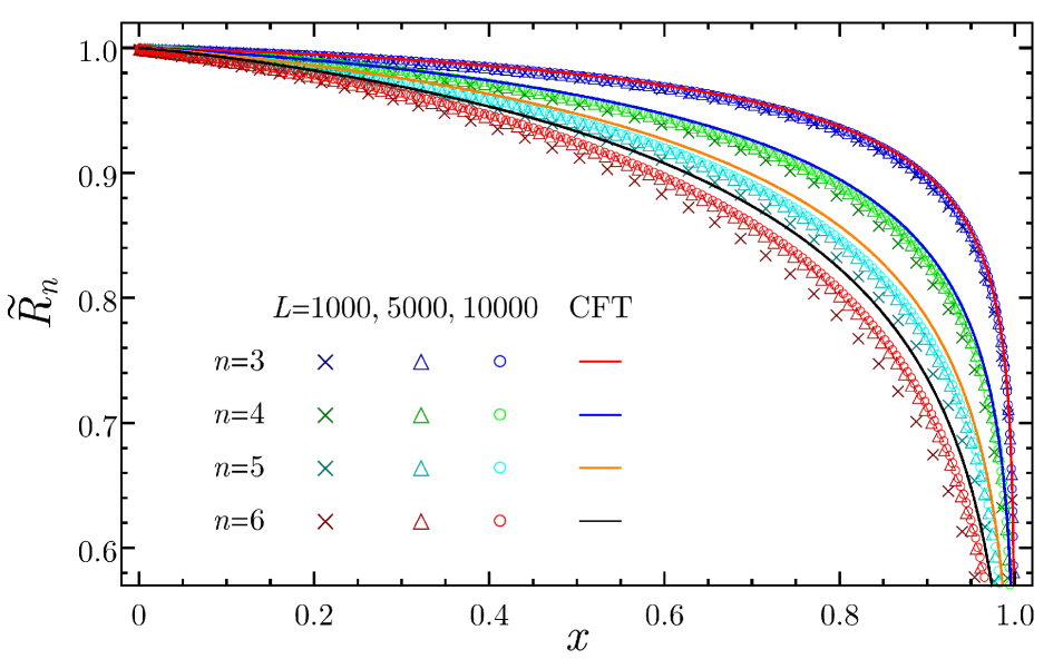
Figure 7: The ratio $\widetilde{R}_{n}(x)$ in (4.5) for the non compact boson. The data points come from the periodic harmonic chain with $\omega L=10^{-5}$, while the curves are given by CFT formula (4.7).

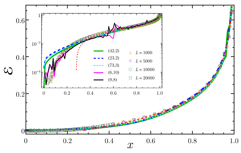
Figure 8: Logarithmic negativity of two disjoint intervals for the non compact boson (4.8) as function of the four-point ratio $x$. The dots are numerical data obtained for the periodic harmonic chains with $\omega L=10^{-5}$ and increasing total lengths. All data collapse on the same curve, which corresponds to the continuum limit. The red dashed curve is the analytic continuation found in [23] in the regime $x\to 1^{-}$. The remaining curves are extrapolations obtained from different rational interpolations having $(p,q)$ indicated. In the inset we show the same plot in logarithmic scale in order to highlight the behaviour of the different extrapolated curves when $x\sim 0$.

In Fig. 7 we compare the CFT result (4.7) for $\widetilde{R}_{n}(x)$ with the corresponding quantity computed for the periodic harmonic chain (3.15), where ${{\rm Tr}}(\rho_{A}^{T_{2}})^{n}$ is computed through the correlators $\langle q_{r}q_{s}\rangle$ and $\langle p_{r}p_{s}\rangle$ as explained in [35]. Notice that we have improved this check with respect to [23], indeed the data in Fig. 7 correspond to chains whose total length $L$ is significantly larger than the ones considered in [23], where $L\leqslant 300$. All the data reported in the figure have $\omega L=10^{-5}$. We have considered also harmonic chains with $\omega L=10^{-3}$ and $L=10000$, finding the same results reported in Fig. 7 for $L=10000$. For $n=3$ the agreement is very good, while it gets worse as $n$ increases. This is expected because of the unusual corrections to the scaling [36].

It is more convenient to consider (4.4) than (4.6) for the computation of the replica limit, and for the logarithmic negativity of the non compact boson we have that [23]

$$\mathcal{E}(x)\,=\,-\frac{1}{2}\log\big{[}K(x)K(1-x)\big{]}-\frac{3}{8}\log(1-x)+\log(\pi/2)-\lim_{n_{e}\rightarrow 1}\sum_{k=1}^{n_{e}/2-1}\log G_{k/n_{e}}(x)\,,$$ (4.8)

where

$$G_{\beta}(x)\,\equiv\,_{2}F_{1}(\beta,\beta,1;x)\left[\,\frac{\Gamma(1-2\beta)}{\Gamma(1-\beta)^{2}}\,(1-x)^{\beta}\,_{2}F_{1}(\beta,\beta,2\beta;1-x)-(\beta\leftrightarrow 1-\beta)\right],$$ (4.9)

being $K(x)$ the elliptic integral of the first kind. The sum in (4.8) is defined for $n_{e}\geqslant 4$ and for $n_{e}=2$ that term is zero. The analytic continuation in (4.8) is not known for the entire range $x\in(0,1)$. In [23] the analytic continuation has been found for the regime $x\to 1^{-}$, obtaining an expression that surprisingly works down to $x\sim 0.3$ (see the dashed red curve in Fig. 8).

Here we numerically extrapolate $\mathcal{E}(x)$ through the formula (4.8) by using the rational interpolation method, which has been discussed in §A and employed in the previous sections for the entanglement entropy of disjoint intervals. It is worth remarking that, since the replica limit (1.7) for $\mathcal{E}(x)$ involves only even $n$’s, to perform a rational interpolation characterized by some $(p,q)$ we need higher values of $n$ with respect to the ones employed for the entanglement entropy in the previous sections. In particular, for the logarithmic negativity $p+q+1\leqslant n_{e,\textrm{\tiny max}}/2$.

In Fig. 8 we report the extrapolations found for some values of $(p,q)$. Since the numerical data from the harmonic chain are accurate enough to provide the curve in the continuum limit that should be found through the analytic continuation (4.8), we can check the reliability of our numerical extrapolations against them. For the non compact boson the expression (4.9) is not difficult to evaluate numerically. Thus, we can deal with high values of $n$ and therefore we have many possibilities for $(p,q)$. It turns out that an accurate extrapolation for the logarithmic negativity requires high values of $p$ and $q$, in particular for the regime of small intervals $x\sim 0$ (see Fig. 11 in §A for extrapolations having low $p$ and $q$). As already remarked in [22, 23], the behaviour of $\mathcal{E}(x)$ when $x\sim 0$ is not power-like. We observed, as a general behaviour, that increasing $q$ leads to extrapolations which are closer to the numerical data, but spurious fluctuations or even singularities in some regimes of $x$ can occur (see the black and magenta curves in the inset of Fig. 8, and the dashed magenta and cyan curves in Fig. 11). This happens whenever one of the $q$ poles of the rational function is close to the range $(1,n_{\textrm{\tiny max}})$ of the interpolated data and not too far from $n=1$ (it may be real or have a small imaginary part). More details are reported in §A. Taking low $q$’s, one usually gets smooth curves but even high values of $p$’s are not sufficient to capture the behaviour of $\mathcal{E}(x)$ when $x\sim 0$.

Thus, the logarithmic negativity is more difficult to find through the rational interpolation method than the entanglement entropy. Indeed, while for the latter one few Rényi entropies are enough to capture the expected result in a stable way, for the logarithmic negativity more input data are needed to reproduce the regime of distant intervals. Maybe other numerical methods are more efficient. It is worth remarking that the fact that high values of $n$’s in ${{\rm Tr}}(\rho_{A}^{T_{2}})^{n}$ are required to perform accurate extrapolations of the logarithmic negativity leads to a computational obstacle whenever $\mathcal{G}_{n}(x)$ in (4.2) is written in terms of Riemann theta functions, like for the compact boson [23] and for the Ising model [27, 28]. Given our computational resources, we have not been able to deal with those analytic expressions for $n$ high enough to guarantee convincing extrapolations.

5 Conclusions

The analytic continuations leading to analytic expressions for the entanglement entropy and the logarithmic negativity of disjoint regions can be very difficult to perform, even for simple CFTs. In this paper we studied this problem numerically for the CFTs given by the free massless boson (compactified or in the decompactification regime) or by the Ising model, where ${\rm Tr}\rho_{A}^{n}$ for a generic number of disjoint intervals [7, 8, 19] and ${\rm Tr}(\rho_{A_{1}\cup A_{2}}^{T_{2}})^{n}$ are known analytically [22, 23, 27, 28].

The numerical extrapolations have been performed through a method based on rational interpolations, which has been first employed in this context by [20]. Its reliability has been checked by reproducing the existing results found from the corresponding lattice models through various techniques like exact diagonalizations [6, 19] and Tree Tensor Networks [9]. In our analysis, we observed that for the entanglement entropy one finds the same curve through different extrapolations already with small values of the degrees $p$ and $q$ of the polynomials occurring in the numerator and in the denominator respectively of the rational interpolation. Instead, for the logarithmic negativity higher values of $p$ and $q$ are needed for the regime of distant intervals, where it falls off faster than any power. Extrapolations having higher values of $q$ are more efficient in providing the expected result, but they can show some spurious behaviour in some parts of the domain. Our numerical analysis has been limited both by our computational resources (in the evaluation of the Riemann theta functions for large matrices) and by the features of the model (e.g. for the logarithmic negativity of distant intervals). These obstacles prevented us to treat some interesting cases like the logarithmic negativity of two disjoint intervals for the compact boson and for the Ising model because high values of $n$ are needed to get convincing extrapolations. We remark that lattice results for $\mathcal{E}(x)$ have been found in [28] for the Ising model through Tree Tensor Networks, while for the compact boson they are not available in the literature (see [37] for $\widetilde{R}_{3}$ obtained through Quantum Monte Carlo).

When singularities in $n$ occur (see e.g. [38]), the numerical method adopted here is expected to fail. As for the one dimensional systems that have been considered, given the good agreement with the lattice results, a posteriori we expect that there are no singularities in the ranges of $n$ that have been explored.

The rational interpolation method has been also employed to address some cases whose corresponding lattice results are not available in the literature (e.g. the $U(1)$ gauge theory in $2+1$ dimensions has been studied in [20] and the case of three disjoint intervals for the Ising model in §3). Thus, it is a useful tool that could be used in future studies to find numerically the entanglement entropy and the logarithmic negativity of disjoint regions (or for single regions whenever the analytic continuation is difficult to obtain) for other interesting situations like e.g. for CFTs in higher dimensions [39] and in the context of the holographic correspondence [12, 13, 40].

Appendices

Appendix A Rational interpolations

In this appendix we discuss the numerical method that we have employed throughout the paper, which is based on rational interpolations, and the issues we encountered to address the replica limits for the entanglement entropy and negativity considered in the main text. Its use in this context has been first suggested in [20].

The rational interpolation method consists in constructing a rational function which interpolates a finite set of given points labeled by a discrete variable. Once the rational function is written, one simply lets the discrete variable assume all real values. The needed extrapolation is found by just evaluating the rational function obtained in this way for the proper value of the variable.

For the quantities we are interested in, the discrete variable is an integer number $n$. As a working example, let us consider the case of two disjoint intervals, where the variable $x\in(0,1)$ characterizes the configuration of intervals. For any integer $n\geqslant 2$ we have a real function of $x$ and typically we have access only to $n\leqslant n_{\textrm{\tiny max}}$ for computational difficulties. The rational function interpolating the given data reads

$$W^{(n)}_{(p,q)}(x)\equiv\frac{P(x;n)}{Q(x;n)}\equiv\frac{a_{0}(x)+a_{1}(x)n+a_{2}(x)n^{2}+\cdots+a_{p}(x)n^{p}}{b_{0}(x)+b_{1}(x)n+b_{2}(x)n^{2}+\cdots+b_{q}(x)n^{q}}\,,$$ (A.1)

being $p\equiv\textrm{deg}(P)$ and $q\equiv\textrm{deg}(Q)$ the degrees of the numerator and of the denominator respectively as polynomials in $n$. The extrapolations are performed pointwise in the domain $x\in(0,1)$. Thus, for any given $x\in(0,1)$, in (A.1) we have $p+q+2$ coefficients to determine. Nevertheless, since we can divide both numerator and denominator by the same number fixing one of them to 1, the number of independent parameters to find is $p+q+1$. Once the coefficients in (A.1) have been found, the extrapolation is easily done by considering $n$ real and setting it to the needed value. It is important to stress that, having access only to a limited number $m$ of data points, we can only perform rational interpolations whose degrees $(p,q)$ are such that $p+q+1\leqslant m$. This method is implemented in Wolfram Mathematica through the Function Approximations package and the command RationalInterpolation.

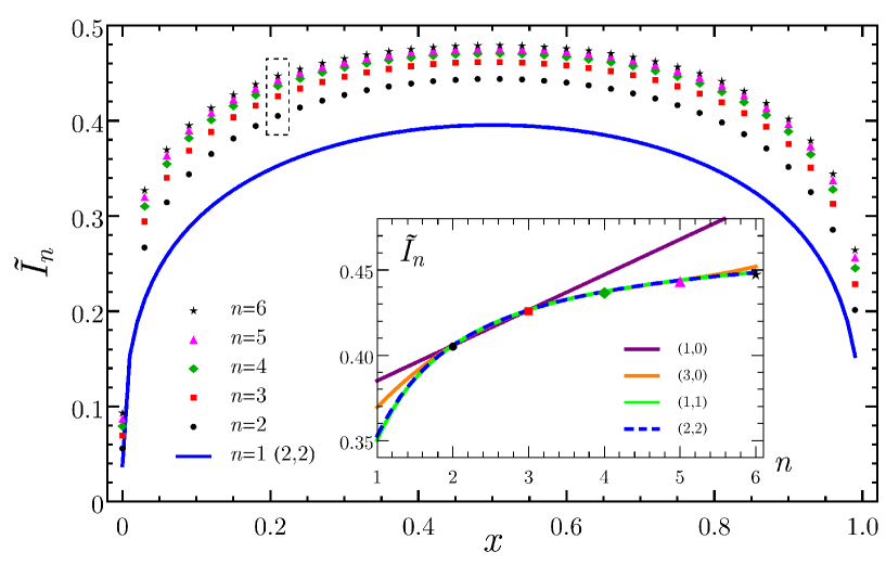
Figure 9: The quantity $\tilde{I}_{n}$ in (2.6) and the corresponding $n\to 1$ limit (2.7) for the compact boson ($c=1$) with $\eta=0.295$. The blue line is the extrapolation $n=1$ of the rational interpolation with $(p,q)=(2,2)$ obtained through the analytic expressions given by (2.10) and (2.11) with $2\leqslant n\leqslant 6$, whose values for $\tilde{I}_{n}$ are shown by points for some values of the four point ratio $x$. In the inset, considering the configuration having $x=0.2101$ (highlighted by the dashed rectangle in the main plot), we show $\tilde{I}_{n}$ as function of $n$ for rational interpolations having different $(p,q)$. The extrapolations having $q>0$ capture the expected value better than the ones having $q=0$.

In Fig. 9 we consider an explicit example where we extrapolate the $\tilde{I}_{1}(x)$ in (2.7) of the compact boson ($c=1$) for a particular value of the compactification radius corresponding to $\eta=0.295$ (see also Fig 2). For $n\geqslant 2$ the analytic expressions are (2.6) and (2.10) and we take into account $2\leqslant n\leqslant 6$ only (in Fig. 2 we employ also $n=7$). Given these data, we can perform rational interpolations with $p+q+1\leqslant 5$. The blue curve in Fig. 9 is the extrapolation to $n=1$ of the rational interpolation with $(p,q)=(2,2)$. We find it instructive to describe the details for a specific value of $x$. Let us consider, for instance, a configuration corresponding to $x=\tilde{x}\equiv 0.2101$ (see the dashed rectangle in Fig. 9). First one has to compute the rational interpolation with $(p,q)=(2,2)$, then the limit $n\to 1$ must be taken. For these two steps, we find respectively

$$W^{n}_{(2,2)}(\tilde{x})=\frac{0.358-0.480\,n+3.689\,n^{2}}{1+1.347\,n+7.870\,n^{2}}\,,\qquad\lim_{n\rightarrow 1}W^{n}_{(2,2)}(\tilde{x})=0.349\,.$$ (A.2)

In the inset of Fig. 9 we show how adding more data improves the final extrapolation and how it becomes stable. Focusing again on $x=\tilde{x}$, we can start by taking only $n\in\{2,3\}$, which allow to perform a rational interpolation with $(p,q)=(1,0)$ (a line). Since rational interpolations having $p=0$ often provide wrong predictions, we prefer to avoid them, if possible. The extrapolation to $n=1$ corresponding to $(p,q)=(1,0)$ cannot be trusted and therefore we consider four input data $n\in\{2,3,4,5\}$ which allow to consider a rational interpolation with, for instance, $(p,q)=(3,0)$ and also $(p,q)=(1,1)$. These two different rational interpolations do not provide the same extrapolation to $n=1$ and therefore we must take into account more input data. Considering $2\leqslant n\leqslant 6$ we can choose also $(p,q)=(2,2)$ finding that the corresponding rational interpolation basically coincides with the one with $(p,q)=(1,1)$ (their difference is of order $10^{-3}$). Thus, the extrapolation to $n=1$ obtained with $(p,q)=(2,2)$ is quite stable. Repeating this analysis for the whole range of $x\in(0,1)$, one can find the blue curve in Fig. 9. As a further check, in Fig. 2 we have used $(p,q)=(3,2)$ using more input data, finding that the final extrapolation is basically the same. Plots like the one shown in the inset of Fig. 9 are very useful to understand the stability of the extrapolation to $n=1$. Increasing the values of $p$ and $q$ in the rational interpolations leads to more precise extrapolations, as expected. Rational interpolations with $q>0$ provide extrapolations which are closer to the expected value with respect to the ones with $q=0$. When $q$ is strictly positive, $q$ poles occur in the complex plane parameterized by $n\in\mathbb{C}$. Nevertheless, if these poles are far enough from the real interval $(1,n_{\textrm{\tiny max}})$ containing all the $n$’s employed as input data for the interpolation, the extrapolations to $n=1$ are reliable. Increasing $q$, we have higher probability that one of the poles is close to the region of interpolation, spoiling the extrapolation. Plotting $W^{n}_{(p,q)}(x)$ as function of $n$ is useful to realize whether this situation occurs (see the inset of Fig. 10 for an explicit example).

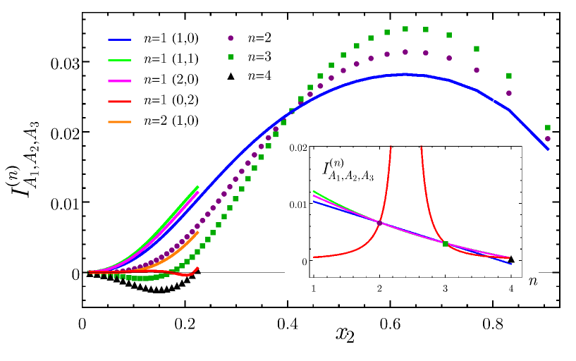
Figure 10: Three disjoint intervals: The quantity $I^{(n)}_{A_{1},A_{2},A_{3}}$ in (3.12) for the compact boson, computed through (3.14) and (3.7) for $n\geqslant 2$. Our limited computational power in evaluating Riemann theta functions for large matrices prevented us to consider $n=4$ in the whole range of configurations and this limits also the possible rational interpolations that can be employed. The blu line is the extrapolation found by using only $n\in\{2,3\}$, which should not be considered as a prediction because more $n$’s are needed to find stable extrapolations. The orange line is a check of the method for $n=2$: the fact that the expected points are not precisely recovered is due to low number of $n$’s ($n\in\{3,4\}$) available. In the inset, considering the configuration having $x_{2}=0.224$, we show $I^{(n)}_{A_{1},A_{2},A_{3}}$ as function of $n$ for rational interpolations having different $(p,q)$. The rational interpolation with $(p,q)=(0,2)$ (red line) shows a bad behaviour and the extrapolation to $n=1$ cannot be trusted; indeed, the red curve in the main plot is different from the other extrapolations.

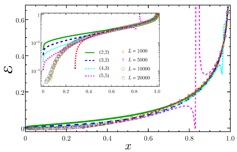
Figure 11: Logarithmic negativity of two disjoint intervals for the non compact boson: Extrapolations having low values of $p$ and $q$. This plot should be compared with Fig. 8, where higher values of $p$ and $q$ have been considered. Increasing $q$ improves the extrapolation but in some regimes of $x$ wrong results can be found. The dashed red curve is the analytic continuation for the regime $x\to 1^{-}$ found in [23], while the points are obtained through a periodic harmonic chain (3.15) with $L$ sites.

The issue of evaluating Riemann theta functions which involve large matrices becomes important when we want to compute $I_{A_{1},A_{2},A_{3}}$ (see (3.11) and (3.12)) for a compact boson. Indeed, $\mathcal{F}_{3,n}(\boldsymbol{x})$ in (3.14) is given by (3.7) for $N=3$ and therefore the matrix occurring in the Riemann theta function is $2g\times 2g$ with $g=2(n-1)$. Given our computational power, we computed $I^{(n)}_{A_{1},A_{2},A_{3}}$ for $n\in\{2,3\}$ for all the needed configurations of intervals, while for $n=4$ we got results only for small intervals. In Fig. 10 we show our data and some numerical extrapolations. In the whole range of $x_{2}$ we performed only the rational interpolation with $(p,q)=(1,0)$ (blue line) because only two input data are available, while for $x_{2}\in(0,0.22)$, where also $n=4$ is available, we could employ higher values of $p$ and $q$. When we have more extrapolations, unfortunately they do not overlap, indicating that we cannot trust these curves to give a prediction, even if they are quite close. Another indication that $n=4$ is not enough to get a precise extrapolation comes from the fact that, given the data with $n\in\{3,4\}$ and extrapolating to $n=2$ (orange curve in Fig. 10) we did not recover exactly the expected values (purple circles) found with the analytic expressions. In the inset we focus on a configuration of three intervals corresponding to $x_{2}=0.224$ and show the dependence of $I^{(n)}_{A_{1},A_{2},A_{3}}$ on $n$ for various $(p,q)$. While the extrapolations to $n=1$ associated to $(1,0)$ (for this one only $n\in\{2,3\}$ have been used), $(1,1)$ and $(2,0)$ are very close, the one corresponding to $(p,q)=(0,2)$ provides a completely different extrapolation to $n=1$. Considering the two poles of the interpolating function in the regime of $x_{2}$ where also $n=4$ is available, we find that they are real and at least one of them is inside the domain $n\in(1,4)$. Thus, the function cannot be considered a good approximation of the true analytic continuation and the extrapolation cannot be trusted. This behaviour does not occur for the case considered in the inset of Fig. 9. Thus, it is useful to plot the $n$ dependence of the functions obtained through the rational interpolation method in order to check the occurrence of singularities that could lead to wrong extrapolations.

We find it instructive to discuss some details about the extrapolations of the logarithmic negativity of two disjoint intervals (see §4). The simplest case we can deal with is the non compact boson and the replica limit to perform for this model is (4.8). The analytic expression (4.9) contains only hypergeometric functions and therefore it can be evaluated for high values of $n$. Some extrapolations performed through the rational interpolation method explained above are shown in Figs. 8 and 11. The first difference between the logarithmic negativity and the mutual information in the extrapolation process is that for the former quantity we need to consider higher values of $p$ and $q$ with respect to the latter one to recover the expected result. Moreover, in the regime of small intervals or large separation (i.e. $x\sim 0$), where the logarithmic negativity falls off to zero faster than any power, it is very difficult to capture its behaviour in a clean way, despite the high values of $p$ and $q$. In Fig. 11 we show some extrapolations characterized by low values of $p$ and $q$. The most difficult regime to capture is the one with $x\sim 0$. Thus, in Fig. 8 we show some extrapolations having higher values of $p$ and $q$. Comparing the curves in these figures, one observes that with low $q$’s it is difficult to capture the regime of small $x$, even for very high values of $p$. Increasing $q$, the agreement slightly improves for small $x$, but, as already remarked, it is more probable that the singularities of the rational interpolation fall close to the domain of the interpolated data. For example, in the case of the dashed magenta curve of Fig.11, all the poles of the rational function are real. Varying the parameter $x$, they move on the real axis and, whenever one of them comes close to the interpolation region $(1,n_{\textrm{\tiny max}})$ and it is not too far from $n=1$, the extrapolated function to $n=1$ cannot be trusted as approximation of the true analytic continuation. This leads to fluctuations or singularities in the extrapolation curve as function of $x$ (e.g. see also the dashed cyan curve in Fig. 11 and the black and magenta curves in Fig. 8).

References

References

-
[1]
L. Amico, R. Fazio, A. Osterloh, and V. Vedral,
Rev. Mod. Phys. 80, 517 (2008);
J. Eisert, M. Cramer, and M. B. Plenio, Rev. Mod. Phys. 82, 277 (2010);
P. Calabrese, J. Cardy, and B. Doyon Eds, J. Phys. A 42 500301 (2009). -
[2]
C. G. Callan and F. Wilczek,
Phys. Lett. B 333, 55 (1994);
C. Holzhey, F. Larsen, and F. Wilczek, Nucl. Phys. B 424, 443 (1994). - [3] P. Calabrese and J. Cardy, J. Stat. Mech. P06002 (2004).
- [4] P. Calabrese and J. Cardy, J. Phys. A 42, 504005 (2009).
- [5] M. Caraglio and F. Gliozzi, JHEP 0811: 076 (2008).
- [6] S. Furukawa, V. Pasquier, and J. Shiraishi, Phys. Rev. Lett. 102, 170602 (2009).
- [7] P. Calabrese, J. Cardy, and E. Tonni, J. Stat. Mech. P11001 (2009).
- [8] P. Calabrese, J. Cardy, and E. Tonni, J. Stat. Mech. P01021 (2011).
- [9] V. Alba, L. Tagliacozzo, and P. Calabrese, Phys. Rev. B 81 060411 (2010).
- [10] M. Fagotti and P. Calabrese, J. Stat. Mech. (2010) P04016.
-
[11]
F. Igloi and I. Peschel,
2010 EPL 89 40001;
V. Alba, L. Tagliacozzo, and P. Calabrese, J. Stat. Mech. (2011) P06012;
M. Rajabpour and F. Gliozzi, J. Stat. Mech. (2012) P02016;
M. Fagotti, EPL 97, 17007 (2012); P. Calabrese, J. Stat. Mech. (2010) P09013. -
[12]
S. Ryu and T. Takayanagi,
Phys. Rev. Lett. 96 (2006) 181602;
S. Ryu and T. Takayanagi, JHEP 0608: 045 (2006). - [13] M. Headrick, Phys. Rev. D 82, 126010 (2010).
-
[14]
F. Alcaraz, M. Berganza and G. Sierra,
Phys. Rev. Lett. 106 (2011) 201601;
M. Berganza, F. Alcaraz and G. Sierra, J. Stat. Mech. (2012) P01016. - [15] L. Taddia, J. Xavier, F. Alcaraz and G. Sierra, Phys. Rev. B 88, 075112 (2013).
-
[16]
F. Essler, A. Lauchli and P. Calabrese,
Phys. Rev. Lett. 110 (2013) 115701;
P. Calabrese, F. Essler and A. Lauchli, J. Stat. Mech. (2014) P09025. - [17] T. Pálmai, Phys. Rev. B 90, 161404 (2014).
- [18] F. Gliozzi and L. Tagliacozzo, J. Stat. Mech. (2010) P01002.
- [19] A. Coser, L. Tagliacozzo, and E. Tonni, J. Stat. Mech. (2014) P01008.
- [20] C. M. Agón, M. Headrick, D. L. Jafferis, S. Kasko, Phys. Rev. D 89, 025018 (2014).
-
[21]
G. Vidal and R. F. Werner, Phys. Rev. A 65, 032314 (2002);
G. Vidal, J. Mod. Opt. 47 (2000) 355;
K. Zyczkowski, P. Horodecki, A. Sanpera and M. Lewenstein, Phys. Rev. A 58, 883 (1998);
A. Peres, Phys. Rev. Lett. 77, 1413 (1996);
J. Eisert, quant-ph/0610253;
J. Eisert and M. B. Plenio, J. Mod. Opt. 46, 145 (1999);
H. Wichterich, J. Molina-Vilaplana and S. bose, Phys. Rev. A 80, 010304 (2009);
S. Marcovitch, A. Retzker, M. B. Plenio and B. Reznik, Phys. Rev. A 80, 012325 (2009). - [22] P. Calabrese, J. Cardy, and E. Tonni, Phys. Rev. Lett. 109, 130502 (2012).
- [23] P. Calabrese, J. Cardy, and E. Tonni, J. Stat. Mech. (2013) P02008.
- [24] P. Calabrese, J. Cardy, and E. Tonni, J. Phys. A48 (2015) 015006
- [25] A. Coser, E. Tonni and P. Calabrese, J. Stat. Mech. P12017 (2014).
-
[26]
V. Eisler and Z. Zimboras,
New J. Phys. 16 (2014) 123020;
M. Hoogeveen and B. Doyon, arXiv:1412.7568;
X. Wen, P.-Y. Chang and S. Ryu, arXiv:1501.00568. - [27] V. Alba, J. Stat. Mech. P05013 (2013).
- [28] P. Calabrese, L. Tagliacozzo and E. Tonni, J. Stat. Mech. P05002 (2013).
- [29] W. Press, S. Teukolsky, W. Vetterling and B. Flannery, Numerical Recipes: The Art of Scientific Computing Cambridge University Press 2007.
- [30] J. Cardy, O. Castro-Alvaredo, and B. Doyon, J. Stat. Phys. 130 (2008) 129.
-
[31]
L. J. Dixon, D. Friedan, E. J. Martinec and S. H. Shenker,
Nucl. Phys. B 282 (1987) 13;
Al. B. Zamolodchikov, Nucl. Phys. B 285 (1987) 481;
L. Alvarez-Gaumé, G. W. Moore and C. Vafa, Commun. Math. Phys. 106 1 (1986);
E. Verlinde and H. Verlinde, Nucl. Phys. B 288 (1987) 357;
V. G. Knizhnik, Commun. Math. Phys. 112, (1987) 567;
M. Bershadsky and A. Radul, Int. J. Mod. Phys. A02, 165 (1987);
R. Dijkgraaf, E. P. Verlinde and H. L. Verlinde, Commun. Math. Phys. 115 (1988) 649. -
[32]
J. Fay,
Theta functions on Riemann surfaces,
Lecture Notes in Mathematics 352,
Springer-Verlag, 1973;
D. Mumford, Tata lectures on Theta III, Progress in Mathematics 97, Birkhäuser, Boston 1991;
J. Igusa, Theta Functions, Springer-Verlag, 1972. - [33] T. Giamarchi, Quantum Physics in One Dimension, Oxford University Press, New York (2004).
- [34] L. Tagliacozzo, G. Evenbly, and G. Vidal, Phys. Rev. B 80 235127 (2009).
-
[35]
I. Peschel and M. C. Chung,
J. Phys. A 32, (1999) 8419;
K. Audenaert, J. Eisert, M. B. Plenio, and R. F. Werner, Phys. Rev. A 66, 042327 (2002);
I. Peschel, J. Phys. A 36, (2003) L205;
A Botero and B. Reznik, Phys. Rev. A 70, 052329 (2004).
M. B. Plenio, J. Eisert, J. Dressig and M. Cramer, Phys. Rev. Lett. 94, 060503 (2005);
M. Cramer, J. Eisert, M. B. Plenio, and J. Dreissig, Phys. Rev. A 73, 012309 (2006);
I. Peschel and V. Eisler, J. Phys. A 42, (2009) 504003. -
[36]
P. Calabrese, M. Campostrini, F. Essler and B. Nienhius,
Phys. Rev. L 104, 095701 (2010);
P. Calabrese and J. Cardy, J. Stat. Mech. P04023 (2010);
P. Calabrese and F. Essler, J. Stat. Mech. P08029 (2010). - [37] C. Chung, V. Alba, L. Bonnes, P. Chen, A. Lauchli, Phys. Rev. B 90, 064401 (2014).
- [38] M. Zaletel, J. Bardarson and J. Moore, Phys. Rev. Lett. 107 (2011) 020402.
-
[39]
J. Cardy,
J. Phys. A 46 (2013) 285402;
H. Casini and M. Huerta, JHEP 0903: 048 (2009);
N. Shiba, JHEP 1207:100 (2012).
H. Schnitzer, arXiv:1406.1161. -
[40]
V. E. Hubeny and M. Rangamani,
JHEP 0803: 006 (2008);
E. Tonni, JHEP 1105:004 (2011);
P. Hayden, M. Headrick and A. Maloney Phys. Rev. D 87, 046003 (2013).
T. Faulkner, arXiv:1303.7221;
T. Hartman, arXiv:1303.6955;
T. Faulkner, A. Lewkowycz, and J. Maldacena, JHEP 1311 (2013) 074.
P. Fonda, L. Giomi, A. Salvio and E. Tonni, arXiv:1411.3608.