Statistical fractal analysis of 25 young star clusters

Abstract

A large sample of young stellar groups is analysed aiming to investigate their clustering properties and dynamical evolution. A comparison of the $\mathcal{Q}$ statistical parameter, measured for the clusters, with the fractal dimension estimated for the projected clouds shows that 52% of the sample has substructures and tends to follow the theoretically expected relation between clusters and clouds, according to calculations for artificial distribution of points. The fractal statistics was also compared to structural parameters revealing that clusters having radial density profile show a trend of parameter $\overline{s}$ increasing with mean surface stellar density. The core radius of the sample, as a function of age, follows a distribution similar to that observed in stellar groups of Milky Way and other galaxies. They also have dynamical age, indicated by their crossing time, that is similar to unbound associations. The statistical analysis allowed us to separate the sample into two groups showing different clustering characteristics. However, they have the same dynamical evolution, since the whole sample has been revealed as expanding objects, for which the substructures seem to have not been erased. These results are in agreement with simulations that adopt low surface densities and models under supervirial conditions.

1 Introduction

It is widely accepted that the physical conditions for the formation and evolution of stellar clusters can be inferred on basis of embedded clusters structure, which depends on the distribution of dense gas of their original cloud. Numerous clusters embedded in clouds are found in the Galaxy. Lada & Lada (2003) suggested that most of them shall lose their dynamical equilibrium, been dissolved in a few tens of Myr. Based on the surface density profile of the distribution of members, they proposed two types of cluster structure: centrally concentrated and hierarchical.

Elmegreen & Falgarone (1996) demonstrated the fractal origin of the relations of size and mass distribution in the interstellar gas, determined from clouds surveys in the literature. More recently, Girichidis et al. (2012) used hydrodynamic simulations of formation of filaments and protostars, in different initial configurations, aiming to evaluate the statistical properties of embedded clusters in the early star-forming phases. They found that more substructures are formed by flat density profiles and compressive modes, instead of to produce centrally concentrated profiles.

Classical open clusters are characterized by a centrally concentrated surface distribution, whose radial profile is smooth and can be reproduced by a simple power law function. On the other hand, hierarchical type clusters show multiple peaks, or substructures in their surface density distribution, like NGC 1333 (Lada, Alves & Lada, 1996), for instance. More recently, Gutermuth et al. (2008) discussed the structure of this cluster based on Spitzer observations of 137 members, whose surface density map shows an elongated distribution, not centrally concentrated, suggesting a low velocity dispersion and that NGC 1333 is not in virial equilibrium.

In spite of the large number of different clusters found in the Galaxy, their relative occurrence remains to be verified, requiring the investigation of clustering properties in a as large as possible sample of studied objects.

For instance, Feigelson et al. (2011) studied the structure of a huge sample of young stars detected by ray-X observations in the Chandra Carina Complex Project (CCCP). They found three different types of clustering properties in their sample that includes previously known clusters and some additional smaller groups identified by CCCP. The classical, centrally concentrated clusters, present an unimodal stellar distribution. Objects showing several substructures, distributed in a circular boundary, are classified as multimodal clumpy structure, which is suggested to be an unequilibrated stage of cluster formation. The third type of cluster contains sparse compact groups, without any concentration that is possibly due to triggered star formation.

The effects of ionizing fronts on triggered star formation have been evaluated using numerical simulations by Walch et al. (2013), for instance.

Considering the rapid changes on the spatial distribution of forming stars shown by these simulations, it is expected a strong evolution of the clustering structure, that can be evaluated by the statistical parameter $\mathcal{Q}$ (Cartwright & Whitworth, 2004). Indeed, a rapid change of $\mathcal{Q}$ is noted in the simulations of ionization-induced star formation by Dale, Ercolano & Bonnell (2012, 2013). However, smooth evolution is also found in the simulations with- and without feedback of ionizing source, depending on the initial conditions (Parker & Dale, 2013; Parker et al., 2014).

Based on fractal statistics, in a previous work we discussed the formation and evolution conditions of four young clusters (Fernandes, Gregorio-Hetem & Hetem, 2012, hereafter FGH12). The preliminary results revealed that one object of the sample has radial stellar density profile that is not similar to the fractal characteristics of the nearby cloud, in a contrary way of the other three studied clusters.

Aiming to validate, refine and enlarge our previous investigation of fractal statistics and its possible relation to the initial conditions of cluster formation, in the present work the analysis is extended to a sample of 21 open star clusters, selected according to their youth and intermediate distances. The clusters were characterized by Santos-Silva & Gregorio-Hetem (2012, hereafter SG12) by using near-infrared data to derive their structural parameters based on stellar density maps, similar to the study developed by Bonatto & Bica (2009), for instance.

The dependence of fractal statistics on age and crossing time was also analysed, aiming to investigate the dynamical evolution that is expected for the star distribution in young clusters, which has been extensively modelled by theoretical simulations (e.g. Cartwright & Whitworth (2004); Goodwin & Whitworth (2004); Parker & Dale (2013); Gieles & Portegies Zwart (2011); Parker et al. (2014); Parker & Andersen (2014); among others). The results were also compared to the observational studies by Schmeja & Klessen (2006), Caballero (2008), Sánchez & Alfaro (2009), Portegies Zwart, McMillan & Gieles (2010, hereafter PZMG10) and Wright et al. (2014), for instance.

The paper is organized as follows. Section 2 is dedicated to present the characteristics of the selected clusters. Section 3 summarizes the adopted methodology, describing the calculations of fractal dimension of clouds, clustering statistics of surface stellar density, and error estimation by using the bootstrap method. Section 4 presents the results from the statistical analysis, and in Sect. 5 the dynamical evolution of the sample is discussed. Finally, the main conclusions are summarized in Sect. 6.

2 Selected star clusters

All the selected young clusters have similar angular sizes ($R<20$ arcmin), and intermediate distances, which is $d\leqslant$ 2 kpc for most of the objects. Since the observed E(B-V) is low, varying from 0.1 to 0.7, we assume that none of them can be considered an embedded cluster.

Table 1 lists the 25 young star clusters analysed in the present work, giving the information available in the literature. For comparison purposes, the four clusters previously studied by FGH12 have been included in the sample. The other 21 clusters have structural and fundamental parameters determined by SG12.

2.1 Observed radial density profile

SG12 used surface stellar density to derive the structural parameters of the clusters. Membership probabilities, evaluated according to proper movement (Dias et al., 2002), were used to identify the very-likely members. SG12 also adopted color-magnitude filters that enable to separate field-stars from candidate members, which were also included in the total number of objects ($N_{T}$) used to determine the stellar density maps.

Table 1 reproduces the structural parameters obtained by SG12 by fitting the observed radial density profile, based on the empirical model from King (1962): $\sigma(r)=\sigma_{bg}+{\sigma_{0}}/({1+(r/r_{c})^{2}})$, where $\sigma(r)$ is the stellar surface density (stars/arcmin²), $\sigma_{bg}$ is the average density measured in a reference region (background), $\sigma_{0}$ and $r_{c}$ are respectively the density and the radius of the cluster core. The cluster radius ($R$) is given by the point where $\sigma(r)=\sigma_{bg}$. The adopted errors are the uncertainties provided by the fitting method. In Sect. 4 these parameters are compared to the statistical fractal parameters obtained in the present work.

Table 1: Sample studied in the present work and informations from literature.

Cluster	$N_{T}$	Age	$d$	$n$	$R$	$r_{c}$
		(Myr)	(pc)	(pc-2)	(pc)	(pc)
Collinder 205	174	5	1800	4.8$\pm$1.9	3.4$\pm$1.2	0.30$\pm$0.03
Hogg 10	88	3	2200	7.6$\pm$1.7	1.9$\pm$0.4	0.46$\pm$0.28
Hogg 22	97	3	1700	9.0$\pm$3.8	1.9$\pm$0.5	1.9$\pm$1.1
Lynga 14	68	3	950	16.7$\pm$7.0	1.1$\pm$0.4	0.22$\pm$0.04
Markarian 38	57	6	1500	6.8$\pm$2.3	1.6$\pm$0.5	0.13$\pm$0.03
NGC 2302	70	3	1700	4.0$\pm$1.4	2.3$\pm$0.5	0.54$\pm$0.10
NGC 2362	124	4	1480	3.3$\pm$1.0	1.9$\pm$0.4	0.26$\pm$0.05
NGC 2367	60	3	2200	2.3$\pm$0.6	2.9$\pm$0.7	0.34$\pm$0.11
NGC 2645	104	5	1800	7.5$\pm$2.1	2.1$\pm$0.5	0.22$\pm$0.04
NGC 2659	215	5	2000	5.2$\pm$0.9	3.6$\pm$0.5	1.93$\pm$0.37
NGC 3572	149	3	1900	7.7$\pm$1.9	2.5$\pm$0.5	0.16$\pm$0.03
NGC 3590	79	3	1680	11.7$\pm$4.5	1.5$\pm$0.4	0.29$\pm$0.06
NGC 5606	98	3	2200	4.8$\pm$0.9	2.6$\pm$0.4	0.51$\pm$0.13
NGC 6178	106	5	1430	12.2$\pm$2.7	1.7$\pm$0.4	0.30$\pm$0.12
NGC 6604	90	6	1600	4.4$\pm$1.3	2.6$\pm$0.7	0.50$\pm$0.11
NGC 6613	133	5	1550	4.9$\pm$1.2	2.9$\pm$0.7	0.12$\pm$0.01
Ruprecht 79	174	5	2700	3.6$\pm$0.5	3.9$\pm$0.5	2.20$\pm$0.80
Stock 13	65	4	2000	3.8$\pm$0.9	2.3$\pm$0.3	0.11$\pm$0.05
Stock 16	139	7	2000	5.8$\pm$1.6	2.8$\pm$0.7	1.20$\pm$0.60
Trumpler 18	164	5	2850	2.5$\pm$0.4	4.6$\pm$0.8	0.38$\pm$0.10
Trumpler 28	73	2	1050	12.3$\pm$4.5	1.4$\pm$0.5	0.84$\pm$0.16
Berkeley 86	85	5	1585	3.4	2.8
NGC 2244	295	3	1660	1.9	7.0
NGC 2264	292	3	760	5.0	4.3
NGC 6530	62	3	1300	2.9	2.6

Note: Data for 21 clusters are given by SG12, and for the last four clusters are from FGH12 and references therein.

2.2 Mass and age

By comparing the cluster members with pre-MS (Siess, Dufour & Forestini, 2000) and main sequence (Girardi et al., 2002) models in the unreddened near-IR colour-magnitude diagrams, SG12 estimated fundamental parameters like age and mass. The mean ages are $\sim 5$ Myr, but some of the clusters have a bimodal age distribution, showing a second peak around 12 Myr (Hogg 22, Lynga 14, NGC 2302, NGC 2645, NGC 5606, and NGC 5606).

The observed mass distribution of each cluster was fitted with the mass function $\phi(m)\propto m^{-(1+\chi)}$ from Kroupa (2001). The $\chi$ values determined by the fitting method indicate that 33% of the sample have low power-law index, comparable to the slope $\chi=0.3\pm 0.5$ assumed by Kroupa (2001) for $M<0.5\rm{M}_{\odot}$. The other 67% of the clusters have deeper slopes $\chi\sim 0.8$ to 1.5 that are, within the errors, roughly similar to the Salpeter’s IMF ($\chi=1.35$), which is the index that Kroupa (2001) suggested for $M>1\rm{M}_{\odot}$. This result is also in agreement with the mass distribution with $\chi\sim 1.0$ that has been found for the initial cluster mass function of diverse clusters (e.g. Elmegreen, 2010; Oey, 2011).

The mean mass of the cluster members is $>1~{}\rm{M}_{\odot}$, indicating an incompleteness of low-mass stars, probably due to the 2MASS detection limit that constrains the presence of faint sources in the sample.

Considering the total mass, it is interesting to note that our sample corresponds to an intermediate range between the embedded clusters studied by Lada & Lada (2003) and the massive “leak” clusters having $R>$ 10 pc in the sample studied by Pfalzner (2011). All of them follow the same mass-radius relation given by $M\sim 118R^{1.3}$. SG12 (see their Fig. 4c) compare the sample with the distribution of clusters analysed by Pfalzner (2011) who proposed that these objects represent the ending of a time sequence, which mass-radius dependence is $M\sim 359R^{1.7}$. However, this power law fitting is significantly different of the distribution mentioned above, found by SG12 for our sample, as well as for the embedded clusters from Lada & Lada (2003) and also for clusters showing $R<$ 10 pc in the sample analysed by Pfalzner (2011).

The results from SG12 favour the interpretation given by Adams et al. (2006) and Adams (2010) suggesting that differences on mass-radius relations are more likely due to different formation conditions instead of a time sequence ending in the massive “leak” clusters proposed by Pfalzner (2011).

A similar conclusion was achieved by FG12 from the estimated volumetric density, which is correlated with cluster radius by $\rho=28R^{-1.7}$, where $\rho$ is given in M_⊙/pc³, which stands for our sample as well as for embedded clusters from Lada & Lada (2003), being quite similar to other studies, like $\rho\propto R^{-1.92}$ found by Camargo, Bonatto & Bica (2010), for instance.

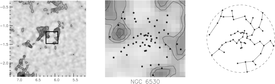
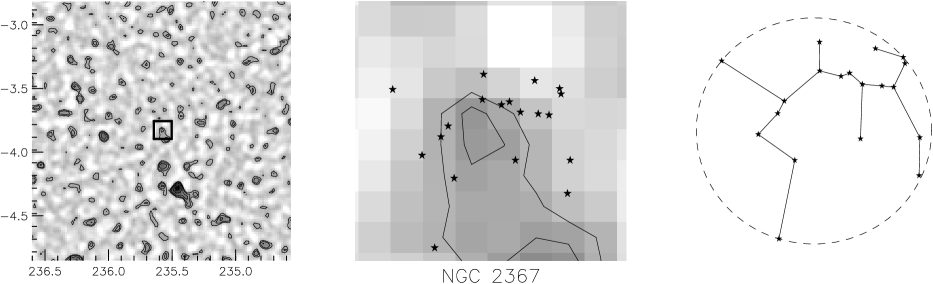
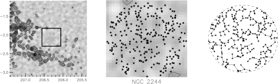
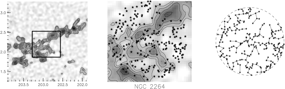
Figure 1: Left: Visual extinction ($A_{V}$) map (galactic coordinates) of nearby clouds of four objects of the sample. Contours represent $A_{V}$ levels with S/N $>$ 10. The location of the star clusters is indicated by the central rectangle. Middle: A zoom of the $A_{V}$ map showing the spatial distribution of the cluster members. Right: Minimal spanning tree and smallest circle (dashed line) that contains all members of the cluster. Upper panels show clusters with $\mathcal{Q}>$ 0.8 (NGC 6530 and NGC 2367), while small scale substructures (NGC 2244 and NGC 2264) are seen in lower panels.

3 Methodology

FGH12 performed fractal analysis of the clusters Berkeley 86, NGC 2244, NGC 2264 and NGC 6530. By comparing with the statistic derived from artificial data simulating stars distributions and parental clouds, the clustering parameters of three of the analysed clusters are compatible with the fractal dimension of the observed clouds. NGC 6530 is the only cluster showing a central concentration of stars that is different of the substructures found for the nearby cloud. In the present work our previous analysis is extended to a larger sample, following the same methodology adopted in FGH12, which is summarized in this section.

3.1 Fractal dimension of the nearby clouds

Visual extinction ($A_{V}$) maps were used to perform statistical analysis of the clouds. Aiming to investigate the interstellar matter distribution in the direction of the clusters, the $A_{V}$ maps were extracted from the Dark Clouds Catalogue presented by Dobashi et al. (2005).

For each cluster we searched for $2^{\rm o}\times 2^{\rm o}$ images containing the $A_{V}$ levels obtained from 2MASS data, with spacial resolution of $\sim 1^{\prime}$ per pixel. A threshold of S/N = 10 was chosen to define the minimum level of $A_{V}$ contour, avoiding low density regions in the calculations. Therefore, $A_{V}$ maps are useful to indicate the presence of dense clouds nearby the cluster.

Figure 1 shows some examples of $A_{V}$ maps and corresponding spatial distribution of cluster members, which were used in the fractal analysis discussed in Sect. 3.2.

Following Hetem & Lépine (1993), the fractal dimension $D_{2}$ of contour levels is measured by using the perimeter-area relation of the clouds $P=({A}^{1/2}/{K})^{D_{2}}$, where $P$ is the perimeter of a given $A_{V}$ contour level and $A$ is the area inside it, and $K$ is a parameter connected to the geometry (shape) of the objects under study. The uncertainties on the estimates of $D_{2}$ and $K$ of projected images of clouds were obtained by applying standard least squares methods (Press et al., 1992).

Since this method uses bi-dimensional projected maps, the comparison of $D_{2}$ with the values of fractal dimension from literature ($D_{3}$), determined from three-dimensional distributions, requires a $3{\rm D}\times 2{\rm D}$ transforming function ($D_{3}={\mathcal{F}}(D_{2})$). Following Falconer (1990), we adopt the relation $D_{3}=D_{2}+1$, which is a good approximation for $D_{3}<2.5$ (Cartwright, Whitworth & Nutter, 2006). However, the relationship between fractal dimension of a cloud projection and three dimensional calculations may depend on a more complex inference of $D_{3}={\mathcal{F}}(D_{2})$ that is not clearly established (Sánchez, Alfaro & P´erez, 2005).

3.2 Clustering statistics

The parameter $\mathcal{Q}$, which carries information about the cluster fractal structure, is a dimensionless quantity given by $\mathcal{Q}=\overline{m}/\overline{s}$, where $\overline{m}$ and $\overline{s}$ are statistical parameters that depend on the geometric distribution of data points (Cartwright & Whitworth, 2004).

The parameter $\overline{m}$ is the normalized mean edge length, related to the surface density of cluster members projected position, defined by:

$$\overline{m}=\frac{1}{(A_{N}N)^{1/2}}\sum_{i=1}^{N-1}{m_{i}}$$

where $N$ is the total number of considered points, $m_{i}$ is the length of edge $i$ in the minimum spanning tree (described below) and $A_{N}$ is the area of the smallest circle that contains all points projected on the plane of the cluster. Each smallest circle was determined by adopting the algorithm proposed by Megiddo (1983).

The minimal spanning tree is defined as the unique network of straight lines that can connect a set of points without closed loops, such that the sum of all the lengths of these lines (or edges) is the minimal possible. Figure 1 gives examples of smallest circle and respective spanning tree, which were constructed using the method described by Gower & Ross (1969) in order to obtain $\overline{m}$ for each cluster.

The value of $\overline{s}$ represents the mean separation of the points, and is given by

$$\overline{s}=\frac{2}{N(N-1)R_{N}}\sum_{i=1}^{N-1}{}\sum_{j=1+i}^{N}|\overrightarrow{r}_{i}-\overrightarrow{r}_{j}|$$

where $r_{i}$ is the vector position of point $i$, and $R_{N}$ is the radius of the smallest circle that contains all points.

Studies of the hierarchical structure in young clusters have used the $\mathcal{Q}$ parameter to distinguish fragmented from smooth distributions (e.g. Elmegreen, 2010). Comparing the cluster physical structure with the geometry of its possible parental cloud may tell us about the original gas distribution of the star forming region and how the particular cloud may have evolved during the cluster formation.

Using artificial distributions of points, Lomax, Whitworth & Cartwright (2011) adopted the technique proposed by Cartwright & Whitworth (2004) to perform a statistical analysis that gives inferences on the fractal dimension measured on grey-scale images generated by models of stars clusters and clouds. They used data sets varying from 64 to 65536 points, which give a parameters space of $\mathcal{Q}$ as a function of radial profiles (index $\alpha$) and fractal dimension ($D_{3}$) that are similar to, but larger than the calculations performed by Cartwright & Whitworth (2004) and Sánchez & Alfaro (2009), for instance. In Sect. 4.2 the results are compared with these theoretical models.

3.3 Standard deviation estimated with bootstrapping

The bootstrap method was adopted in order to estimate the standard deviation of the statistical parameters. This numerical method, introduced by Efron (1979), is independent of model or calculations; is not based on asymptotic results; and is simple enough to be automatized as an algorithm. The method creates a set of simulated data by considering each parameter of the model as varying in a chosen confidence level according to a given distribution. Then, this artificial set is treated as a real sample (as those obtained by observations) and the standard deviation is calculated from these data.

In the present work, the bootstrapping algorithm was implemented as proposed by Press et al. (1992). The algorithm generates synthetic distributions of cluster members based on the original positions of the stars. A number of stars is moved from their original positions, being replaced by random points within a box, around the star, with side equals to the cluster radius. Then, the parameters $\overline{m}$, $\overline{s}$ and $\mathcal{Q}$ are calculated for each synthetic distribution. By adopting a fraction $f=1/e\sim 37\%$ of replaced stars in a symmetric normal distribution, it was possible to derive $1\sigma$ deviation for $\mathcal{Q}$, $\overline{m}$ and $\overline{s}$.

Figure 2: Distribution of $\mathcal{Q}$ as a function of number of stars (top axis) and membership probability (bottom axis) calculated for members and candidate members of NGC 2244. The limiting values adopted in the present work, $N=256$ and $P=50\%$, are shown by a dashed line.

4 Analysis of fractal statistics

4.1 Membership dependence

In spite of the whole set of stars (candidates and members) had been used by SG12 to determine the cluster structural parameters, in the present work we preferred to constrain the statistical analysis to confirmed members only. Based on the probability membership ($P\%$), the stars were separated in two sub-samples: the very likely members of the cluster have $P\geq 50\%$ (denoted by $P_{m}$), while the candidate members (called $P_{c}$) have $P<50\%$ .

Aiming to evaluate the effect on the fractal statistics by considering different numbers of stars and to explore the validity in choosing $P_{m}$ to represent the very likely members, Fig. 2 shows the variation of $\mathcal{Q}$ as a function of $N$ for the cluster NGC 2244. The adopted result $\mathcal{Q}=0.74$ obtained for $N=256$ members is plotted with error bars. It can be seen that this result stands as a representative value for almost the whole data set, with a smooth decreasing for low numbers of stars. A significant change in $\mathcal{Q}$ occurs only for $N=14$ members with $P>80\%$, but the main conclusion about the clustering structure of NGC 2244 remains the same.

Figure 2 also displays the variation of $\mathcal{Q}$ as a function of the membership probability. This distribution shows that the choice of $P_{m}$ is good enough to avoid large errors due to a small data set (low $N$), also excluding possible field-stars contamination (low $P\%$).

For each set of stars ($P_{m}$ and $P_{c}$ sub-samples), we performed the calculation of the parameters $\overline{m}$ and $\overline{s}$, which are displayed in Fig. 3. It can be seen that the distribution of $P_{m}$ members in this plot tend to follow the expected correlation between $\overline{m}$ and $\overline{s}$, while the candidate members do not follow the same distribution, probably due to field-stars contamination.

For comparison with literature, other objects are also included in Fig. 3, like $\rho$ Oph, Taurus, Chamaeleon, IC 348, Serpens (Schmeja & Klessen, 2006), and IC 2391 which was analysed by Cartwright & Whitworth (2004) along with the first four clusters mentioned above. In spite of the agreement on the $\mathcal{Q}$ values between both works, their results on $\overline{m}$ and $\overline{s}$ differ in almost 20%, excepting Taurus for which the $\overline{m}$ values are 50% discrepant.

Since the cluster $\sigma$ Ori (Caballero, 2008) has available parameters that can be used in several of our comparative plots, a different symbol is used distinguishing it of other clusters from literature.

Figure 3: Trend of $\overline{m}$ increasing with $\overline{s}$ shown by the very likely members of the sample (SG12 and FGH12). Candidate members ($P_{c}$) do not follow this trend that is illustrated by $\mathcal{Q}=0.8$ (full line) and 10% deviation (dashed lines). Data for other clusters from literature are also plotted for comparison (see Sect. 4.1). Filled symbols represent $\mathcal{Q}<0.8$.

4.2 Cluster structure compared with projected clouds

Table 2 gives the statistical parameters, along with the number of studied stars in each cluster, and an estimation of galactic coordinates (l,b).

Aiming to derive the size of the area occupied by the $P_{m}$ members, we determined the mean (l,b) that give the center of the stellar spatial distribution. The respective dispersion is used to estimate the observed sizes, which show a circular symmetry ($\Delta l\sim\Delta b$) suggesting that our objects are not elongated.

In Fig. 4 the parameter $\mathcal{Q}$, obtained from the $P_{m}$ spatial distribution, is compared with the fractal dimension of the nearby clouds (discussed in Sect. 3.1). The locus of statistical parameters calculated for artificial data points (Lomax, Whitworth & Cartwright, 2011) is shown as a shaded area. Above $\mathcal{Q}$ = 0.8 (dotted line) the shaded area shows the dependence on radial profiles (index $\alpha$), while the variation of fractal dimension ($D_{3}$) is found below this line. Since the index $\alpha$ was not estimated for our objects, the upper region of Fig. 4 is displayed only for comparison with other theoretical results (Sánchez & Alfaro, 2009)(full lines). They are also comparable to simulations for cluster types F2.0 to F3.0 and 3D0 to 3D2.9 from Cartwright & Whitworth (2004), which respectively correspond to fractal and radial distributions.

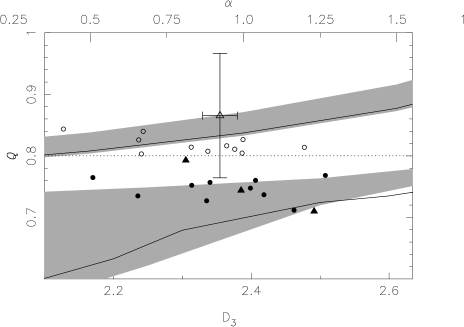
Figure 4: Parameter $\mathcal{Q}$, estimated from the spatial distribution of cluster members, as a function of fractal dimension ($D_{3}$) of projected clouds. Typical error bars are shown for NGC 6530. For comparison, clustering statistics obtained for artificial data (shaded areas) and other theoretical results (full lines) are also shown.

It can be noted that 43% of the sample is found around the bottom shaded area of Fig. 4, meaning that substructures observed for these clusters ($\mathcal{Q}<$ 0.8) coincide with the fractal characteristics of the projected clouds ($D_{3}<2.5)$. It is important to stress that this is not necessarily a clue for physical relation with the nearby cloud. The meaning of these clusters coinciding with the theoretically expected $\mathcal{Q}\times D_{3}$ parameters space is a possible similarity of the substructures found for the clusters and the clouds that are projected in their direction.

The opposite occurs for the clusters that have $\mathcal{Q}>0.8$ (empty circles), including NGC 6530 (indicated by error bars), which do not show the same clustering structure observed in the projected clouds. The values of $\mathcal{Q}$ obtained for these clusters suggest they are more centrally concentrated, while the nearby clouds have small scale substructures.

In fact, the original geometric structure of the gas distribution is expected no longer be the same of the remaining cloud after the cluster formation. It also depends on the initial conditions of the star-forming environment. Furthermore, the investigation of clusters evolution requires an estimate of their dynamical age, in order to verify if their initial structure should have been erased or not (see discussion in Sect. 5).

Figure 5: Mean surface density compared to $\overline{s}$, which varies more with radial clustering. Symbols are the same as Fig. 3. A trend of $\overline{s}$ increasing with $n$ is observed only for clusters with $\mathcal{Q}>0.8$.

4.3 Surface density

The structural parameters calculated by SG12 were compared to $\mathcal{Q}$, but no special trend was found for most of them.

We also searched for correlations among structural parameters compared to the clustering parameters $\overline{m}$ and $\overline{s}$ in separate. With the exception of NGC 3572 and $\sigma$ Orion, a trend was found for clusters having $\mathcal{Q}>0.8$, which show $\overline{s}$ increasing with average surface density $n$ (number of stars per pc²). The same does not occur for the other clusters that have substructures, as seen in the $n\times\overline{s}$ plot of Fig. 5. Also, no trend was found in the comparisons with $\overline{m}$. These are expected results, since $\overline{s}$ is more sensitive to radial clustering, while $\overline{m}$ varies more under the presence of substructures (Cartwright & Whitworth, 2004).

In order to investigate if clustering is related to the cluster concentration parameter, which is given by tidal radius over core radius, the results were compared to the relation $\mathcal{Q}$ vs. $log(R_{t}/r_{c})$ obtained by Sánchez & Alfaro (2009).

According to the definition, $r_{c}$ is the radius at which the surface brightness drops by a factor of two from the central value (PZMG10).

The tidal radius of the sample was estimated by using the relation suggested by Saurin, Bica & Bonatto (2012): $R_{t}=({M}/{M_{gal}})^{1/3}d_{GC}$, with $M_{gal}={V^{2}_{GC}d_{GC}}/{G}$, where $d_{GC}$ is the distance of the cluster to the Galactic center, $V_{GC}$ = 254 km/s and $R_{GC}$ = 8.4 kpc (Reid et al., 2009). The values of $R_{t}$ are in the range of 7.6 to 13 pc, which give concentration parameter $log(R_{t}/r_{c})$ that varies from 0.7 to 2, independently of $\mathcal{Q}$.

Sánchez & Alfaro (2009) analysed a sample of Galactic open clusters. For the subsample with $\mathcal{Q}>$ 0.8 they found a correlation that is not confirmed by our clusters. Contrary to their results, the distribution of all objects in the sample is not distinguished, having a behaviour similar to the fractal-like subsample analysed by them. The same is noted for $\sigma$ Ori (Caballero, 2008) that has $R_{t}$=21 pc, $r_{c}$=1 pc and $\mathcal{Q}$=0.88. These results possibly indicate that our sample is not tidally limited, meaning that tidal radius is not well defined for them. Yet, $R_{t}$ estimates depend on many assumptions having large error bars. For this reason, we preferred not using tidal radius in the present analysis.

Table 2: Results from fractal analysis

cluster	$l^{\rm o}$	$\Delta l$	$b^{\rm o}$	$\Delta b$	$N$	$\mathcal{Q}$	$\overline{m}$	$\overline{s}$	$D_{2}$	$T_{cr}$ (Myr)
Collinder 205	269.21	0.12	-1.85	0.11	34	0.84$\pm$0.12	0.65$\pm$0.21	0.77$\pm$0.30	1.13$\pm$0.05	47.4
Hogg 10	290.8	0.05	0.08	0.05	18	0.80$\pm$0.12	0.79$\pm$0.40	0.98$\pm$0.53	1.24$\pm$0.09	26.5
Hogg 22	338.56	0.07	-1.14	0.06	23	0.81$\pm$0.11	0.76$\pm$0.38	0.94$\pm$0.49	1.38$\pm$0.03	23.1
Lynga 14	340.92	0.07	-1.09	0.07	15	0.75$\pm$0.18	0.74$\pm$0.32	0.99$\pm$0.53	1.40$\pm$0.03	15.3
Markarian 38	11.98	0.06	-0.93	0.06	15	0.75$\pm$0.19	0.67$\pm$0.22	0.89$\pm$0.35	1.31$\pm$0.06	25.8
NGC 2302	219.3	0.07	-3.12	0.07	30	0.76$\pm$0.15	0.67$\pm$0.25	0.88$\pm$0.42	1.17$\pm$0.05	40.2
NGC 2362	238.17	0.07	-5.55	0.06	22	0.81$\pm$0.11	0.74$\pm$0.30	0.91$\pm$0.37	1.34$\pm$0.07	21.4
NGC 2367	235.59	0.07	-3.83	0.07	19	0.81$\pm$0.14	0.69$\pm$0.25	0.84$\pm$0.36	1.48$\pm$0.04	59.2
NGC 2645	264.8	0.07	-2.9	0.08	28	0.80$\pm$0.12	0.72$\pm$0.29	0.90$\pm$0.43	1.39$\pm$0.04	29.4
NGC 2659	264.18	0.11	-1.65	0.11	55	0.83$\pm$0.12	0.73$\pm$0.27	0.88$\pm$0.40	1.39$\pm$0.04	45.8
NGC 3572	290.71	0.07	0.2	0.07	29	0.83$\pm$0.13	0.64$\pm$0.17	0.77$\pm$0.26	1.24$\pm$0.10	30.6
NGC 3590	291.21	0.05	-0.17	0.05	13	0.84$\pm$0.17	0.83$\pm$0.44	0.99$\pm$0.45	1.24$\pm$0.09	20.7
NGC 5606	314.85	0.06	0.99	0.07	32	0.82$\pm$0.14	0.75$\pm$0.32	0.92$\pm$0.47	1.36$\pm$0.04	38.6
NGC 6178	338.41	0.08	1.21	0.07	21	0.76$\pm$0.15	0.72$\pm$0.29	0.95$\pm$0.48	1.34$\pm$0.03	22.3
NGC 6604	18.25	0.09	1.7	0.1	33	0.74$\pm$0.19	0.65$\pm$0.19	0.89$\pm$0.40	1.42$\pm$0.03	37.5
NGC 6613	14.18	0.11	-1.01	0.1	31	0.73$\pm$0.21	0.71$\pm$0.28	0.98$\pm$0.55	1.34$\pm$0.02	39.7
Ruprecht 79	277.1	0.08	-0.82	0.09	53	0.77$\pm$0.15	0.72$\pm$0.27	0.93$\pm$0.45	1.51$\pm$0.04	53.6
Stock 13	290.5	0.06	1.59	0.07	9	0.71$\pm$0.17	0.79$\pm$0.44	1.12$\pm$0.63	1.46$\pm$0.04	38.9
Stock 16	306.15	0.09	0.06	0.08	19	0.76$\pm$0.16	0.73$\pm$0.32	0.96$\pm$0.52	1.41$\pm$0.05	43.9
Trumpler 18	290.98	0.09	-0.14	0.09	86	0.73$\pm$0.19	0.67$\pm$0.19	0.91$\pm$0.40	1.24$\pm$0.10	65.1
Trumpler 28	356.01	0.07	-0.31	0.07	17	0.81$\pm$0.11	0.87$\pm$0.55	1.06$\pm$0.69	1.31$\pm$0.04	18.5
Berkeley 86	76.66	0.08	1.28	0.08	48	0.79$\pm$0.14	0.73$\pm$0.30	0.92$\pm$0.47	1.31$\pm$0.04
NGC 2244	206.31	0.25	-2.06	0.24	256	0.74$\pm$0.14	0.68$\pm$0.13	0.91$\pm$0.27	1.39$\pm$0.05
NGC 2264	202.92	0.36	2.18	0.33	225	0.71$\pm$0.16	0.66$\pm$0.14	0.93$\pm$0.30	1.49$\pm$0.03
NGC 6530	6.08	0.13	-1.32	0.12	55	0.87$\pm$0.10	0.66$\pm$0.20	0.77$\pm$0.28	1.35$\pm$0.03

Notes: The center of the spatial distribution of the cluster members is indicated in Columns 2-5 showing average galactic coordinates and respective $2\sigma$ deviations ($\Delta l$ and $\Delta b$), which roughly indicate the cluster radius.

5 Dynamical Evolution

No special trend was found when comparing statistical parameters with mass and age of the clusters from SG12. This unexpected lack of correlation is probably due to the similarities observed in their fundamental parameters.

Therefore, the analysis of age dependence on cluster structure is better illustrated by comparing the sample with objects spread in a larger range of fundamental parameters values, like the young massive clusters (YMC) and stellar associations of Milky Way and other galaxies, using data available in Tables 2 to 4 of PZMG10, for instance. Also in this section, the $\mathcal{Q}$ evolution and the crossing time as a function of age are compared with observations and theoretical results from literature.

5.1 Core radius vs Age

It is noted in Fig. 6 that the sample has age and core radius consistent with the Milky Way YMCs, but a large dispersion is observed. The inclusion of our objects, as well as $\sigma$ Ori, in this distribution makes less clear the expected trend of $r_{c}$ increasing with age. However, our results confirm the prediction by PZMG10 that young clusters with large $r_{c}$ probably were missing in their sample, due to a selection bias.

It is also interesting to note that our sample tends to fill the upper region in Fig. 6 (large $r_{c}$ values) that is the expected locus of unbound associations, for which there are more available data of size than $r_{c}$ (see Fig. 8 (left) of PZMG10).

The hypothesis that our clusters probably are expanding objects can be confirmed based on their dynamical evolution. In the following subsection, the size and mass estimated by SG12, were used to investigate how many crossing times the clusters have undergone, which gives an indication on how dynamically evolved they are.

Figure 6: Core radius as a function of age of our clusters (SG12, filled symbols for $\mathcal{Q}<$0.8) and $\sigma$ Ori, compared to Associations and Young Massive Clusters of Milky Way (MW), and clusters of other galaxies of the Local Group (LG) and outside the LG.

5.2 Crossing time

By using the total mass ($M$) and cluster radius ($R$) from SG12, the crossing time of the clusters were estimated adopting the expression $T_{cr}=10({R^{3}}/{GM})^{1/2}$ from Gieles & Portegies Zwart (2011). They suggested a boundary distinguishing stellar groups under different dynamical conditions that is expressed by the “dynamical age”, also called parameter $\Pi$, which is given by the ratio of age and crossing time. Unbound associations (expanding objects) have $\Pi<$ 1, while bound star clusters have $\Pi>$ 1.

For comparison among different samples, in Fig. 7 the dynamical time ($T_{dyn}$) given by PZMG10 was adopted, assuming that $T_{cr}=2.8T_{dyn}$ (Gieles & Portegies Zwart, 2011). The Milky Way stellar groups are presented in two distinct distributions: Associations ($\Pi<1$) and YMCs ($\Pi>1$). In general, the objects in other Local Group galaxies, like LMC, SMC and M31, as well as outside the Local Group, seem to follow the same distribution as YMCs of Milky Way, but are more scattered.

Figure  7 clearly shows that all clusters of the sample are more likely associations, following the same trend of Milky Way objects having $\Pi<$ 1 that corresponds to unbound expanding groups. No differences are found when comparing $\Pi$ with the clustering characteristics of our sample, meaning that both fractal and smooth radial density profile types of objects follow the same age vs. crossing time correlation.

Among the clusters studied by Cartwright & Whitworth (2004), Taurus ($\Pi$ = 0.1) coincides with the distribution shown by our sample and other associations, while $\rho$ Oph ($\Pi$ = 1.5) and Chamaeleon ($\Pi$ = 0.74) are closer to IC 348, which is in the transition region ($\Pi$ = 1). IC 2391 ($\Pi$ = 21.2) is found in the region occupied by older clusters of other galaxies. The scattering observed in this region is probably due to observational difficulties to determine accurate effective radius of distant objects. Our sample is not affected by this observational constraint.

5.3 Clustering Evolution

The values of $\mathcal{Q}$ and age, observed in the sample, were compared with different YSOs classes analysed by Schmeja & Klessen (2006). We noted that $\mathcal{Q}$ values of our clusters are systematically above those obtained with 3D calculations ($\mathcal{Q}\sim 0.7$) for the YSOs in the same range of ages (2 to 7 Myr). Schmeja & Klessen (2006, see their Fig. 5) suggest that 3D-$\mathcal{Q}$ values tend to be lower than the projected 2D calculations. Indeed, a better agreement is found by comparing the results with the calculations for the projections in 2D plans presented by Schmeja & Klessen (2006).

Figure 7: Distribution of age vs. crossing time. The sample is compared to results from Cartwright & Whitworth (2004) (✩) and from PZMG10 (same symbols as Fig. 6). The groups of Milky Way show two distributions: bound YMCs ($+$) and unbound associations ($\times$), separated by a dotted line ($\Pi=1$).

Figure 8: Distribution of $\mathcal{Q}$ as a function of age for the sample and other clusters (same as Fig. 3). Cygnus OB2 is indicated with error bars. The results are compared to the simulations with feedback (solid lines) and without feedback (dashed lines), indicating the initial densities (number of stars per pc²) for some of the models adapted from Parker & Dale (2013).

Considering that the evolution of clustering structure may be affected by the initial star-forming conditions, in Fig. 8 the results are compared with the calculations from Parker & Dale (2013, see their Fig. 3) that used models with- and without feedback to simulate the effects of the presence (or not) of ionizing sources affecting the star formation (Dale, Ercolano & Bonnell, 2012, 2013). Even taking in account the large error bars on $\mathcal{Q}$, as illustrated in Fig. 4, the distribution of $\mathcal{Q}$ values in the sample, as a function of age, is consistent with feedback models, in particular those assuming low initial densities ($\Sigma_{1}$ = 0.6 to 83 stars pc^-2). Parker & Dale (2013) suggest that the lowest density models are the mostly affected by feedback, which are the only ones retaining some substructure for 5 to 10 Myr. Since clusters with low densities have longer relaxation times, their substructures are not erased due to negligible stellar mixing.

Other young clusters from literature were also included in Fig. 8. Excepting Cygnus OB2 (Wright et al., 2014), the other clusters like $\rho$ Oph, Taurus, Chamaeleon, IC348 (Schmeja & Klessen, 2006), and $\sigma$ Ori (Caballero, 2008) are similar to our sample, coinciding with low density feedback models from Dale, Ercolano & Bonnell (2012, 2013).

The results are also comparable to those from Parker et al. (2014) for the evolution of $\mathcal{Q}$ based on simulations of different values of virial ratio $\alpha_{vir}$, the total kinetic energy over the potential energy. Our clusters have a distribution very similar to the simulation of $\alpha_{vir}$ = 1.5 (see their Fig. 3g,h,i), which represents a globally supervirial fractal that is “hot” and unbound, according the terminology introduced by them. The same is found for Cygnus OB2, a very substructured cluster ($\mathcal{Q}=0.4$), which is better represented by calculations for unbound regions under supervirial conditions (Wright et al., 2014).

6 Conclusions

In the present work, the methodology used by FGH12 was adopted to perform a fractal analysis of the sample studied by SG12, aiming to enlarge our previous study for the clusters NCG 6530, Berkeley 86, NGC 2244, and NGC 2264. About half of the sample (52%) shows substructures, indicated by the measured parameter $\mathcal{Q}<0.8$, while the other 48% of the objects are centrally concentrated ($\mathcal{Q}>0.8$). According to Parker et al. (2014), regions having low $\mathcal{Q}$ ($\mathcal{Q}<0.8$ or 1) must be dynamically young.

The projected spatial distribution of very likely members, which have membership probability $P>50\%$, shows a $\overline{m}$ vs. $\overline{s}$ correlation that is confirmed by results from literature for other young clusters. On the other hand, the sub-sample of candidate members ($P<50\%$) do not follow this trend.

Centrally concentrated clusters of the sample have $\overline{s}$ increasing with the mean spatial density (n), which is an expected result since $\overline{s}$ shows more variation for radial clustering. This could also be the explanation for the lack of trend in the n vs. $\overline{s}$ for objects with fractal clustering. However, $\sigma$ Ori shows a too high surface density, being out of the correlation with $\overline{s}$ found by us. This discrepancy is possibly due to uncertainties on the parameters adopted for $\sigma$ Ori ($N_{T}$ = 340 or $R$ = 3 pc).

Visual extinction maps of clouds nearby the clusters were used in order to study the geometric structure of gas and dust distribution, by measuring their fractal dimension $D_{2}$. A transform function was adopted to compare the results, measured on projected 2D maps, with simulations based on 3D models. Intermediate values $2.1<D_{3}<2.5$ were found, which correspond more likely to substructures than to smooth radial profiles.

The distribution of fractal dimension $D_{3}$ (estimated for the observed clouds) as a function of $\mathcal{Q}$ parameter (measured for the clusters) shows that half of the sample tends to follow a theoretically expected $\mathcal{Q}$ $\times~{}D_{3}$ relation, calculated for artificial data (Cartwright & Whitworth, 2004; Sánchez & Alfaro, 2009). These clusters have $\mathcal{Q}<0.78$ that indicates the presence of substructures, similar to those observed in the nearby clouds. On the other hand, 12 clusters (48%), among them NGC 6530, have $\mathcal{Q}>0.8$, which corresponds to radial distribution of stars that does not coincide with the structure of the clouds.

It should be expected that these two groups of clusters could have had different virial conditions in the early formation, which are related to different thermal paths: cold collapse for objects centrally concentrated, or warm collapse for those showing substructures (Delgado et al., 2013). Therefore, differences on dynamical evolution could also be expected, but they were not observed for these two subsamples.

The analysis of dependence of age on parameters like core radius and crossing time show that our clusters have many similarities among each other. They are also similar to other young stellar groups of Milky Way, in particular the unbound associations, as indicated by the dynamical ages $\Pi<1$ found for the entire sample.

By comparing the evolution of $\mathcal{Q}$ with theoretical studies, the clusters show a distribution similar to simulations that include feedback of ionizing source in the models adopted by Parker & Dale (2013). According these authors, the calculations using low values of density are the mostly affected by feedback, corresponding to the only simulations retaining some substructure for 5 to 10 Myr, which appears to be the case of our sample. Other young clusters from literature also coincide with these models. A slight tendency is observed for objects that have smooth density profile ($\mathcal{Q}>0.8$), like IC 348 and $\rho$ Oph, being more similar to the calculation with $\Sigma_{i}$ = 24 stars pc^-2. On the other side, Taurus, which shows fractal structure, coincides with the $\Sigma_{i}$ = 0.6 stars pc^-2 model. Our objects are found in between this range of densities.

The observed distribution of $\mathcal{Q}$ as a function of age was also compared to the simulations by Parker et al. (2014) assuming different values of virial ratio ($\alpha_{vir}$). The results are quite similar to the calculations that use $\alpha_{vir}=1.5$, corresponding to “supervirial” fractal.

Since no difference concerning the $\mathcal{Q}$ evolution is noted for our objects, independently if they are fractal or have radial density profile, it is not evident to state if they had or not similar conditions in the early formation.

Additional discussions on the cluster formation conditions must include the initial density distribution of parental clouds, as well as the effects of turbulence. According Girichidis et al. (2012), compressive modes in a flat density profiles tend to form substructures, instead of centrally concentrated distributions of stars. The fractal dimension calculated for clouds, projected in the direction of the studied clusters, allow us to infer the geometric distribution of the dense regions. A more detailed study on dynamical conditions of the gas is required to better understand the scenario of clusters formation and their relation with their parental clouds.

References

- Adams et al. (2006) Adams, F. C., Porszkow, E. M., Fatuzzo, M., Myers, P. C., 2006, APJ 641, 504
- Adams (2010) Adams, F. C. 2010, ARA&A 48, 47
- Bonatto & Bica (2009) Bonatto, C., Santos, J. F. C., Bica, E. 2006, A&A 445, 567
- Caballero (2008) Caballero, J. A. 2008, MNRAS 383, 375-382
- Camargo, Bonatto & Bica (2010) Camargo, D.; Bonatto, C.; Bica, E. 2010, A&A 521, A42
- Cartwright & Whitworth (2004) Cartwright, A., & Whitworth, A. P., 2004, MNRAS 348, 589
- Cartwright, Whitworth & Nutter (2006) Cartwright, A., Whitworth, A. P., Nutter, D. 2006, MNRAS, 369, 1411
- Dale, Ercolano & Bonnell (2012) Dale, J. E., Ercolano, B., Bonnell, I. A. 2012, MNRAS 424, 377
- Dale, Ercolano & Bonnell (2013) Dale, J. E., Ercolano, B., Bonnell, I. A. 2013, MNRAS 430, 234
- Delgado et al. (2013) Delgado, A. J., Djupvik, A. A., Costado, M. T., Alfaro, E.J., 2013 MNRAS 435, 429
- Dias et al. (2002) Dias, W. S., Alessi, B. S., Moitinho, A., & Lépine, J. R. D. 2002, A&A 389, 871
- Dobashi et al. (2005) Dobashi, K., Uehara, H., Kandori, R., Sakurai, T., Kaiden, M., Umemoto, T., & Sato, F. 2005, PASJ, 57, 1
- Efron (1979) Efron, B. 1979, Bootstrap Methods: Another Look At the Jackknife, The Annals of Statistics 7, 126.
- Elmegreen (2010) Elmegreen, B. G., 2010, in Star Clusters: basic galactic building blocks, Proceedings of IAU Symp. No. 266, 2009, R. de Grijs & J. R. D. Lépine, eds., p. 3