Optimal Signaling of MISO Full-Duplex Two-Way Wireless Channel

Abstract

We model the self-interference in a multiple input single output (MISO) full-duplex two-way channel and evaluate the achievable rate region. We formulate the boundary of the achievable rate region termed as the Pareto boundary by a family of coupled, non-convex optimization problems. Our main contribution is decoupling and reformulating the original non-convex optimization problems to a family of convex semidefinite programming problems. For a MISO full-duplex two-way channel, we prove that beamforming is an optimal transmission strategy which can achieve any point on the Pareto boundary. Furthermore, we present a closed-form expression for the optimal beamforming weights. In our numerical examples we quantify gains in the achievable rates of the proposed beamforming over the zero-forcing beamforming.

I Introduction

A node in full-duplex mode can simultaneously transmit and receive in the same frequency band. Therefore, the wireless channel between two full-duplex nodes can be bidirectional, having the potential to double the spectral efficiency when compared to the half-duplex network. Due to the proximity of the transmitters and receivers on a node, the overwhelming self-interference becomes the fundamental challenge in implementing a full-duplex network. The mitigation of the self-interference signal can be managed at each step of the communication network by passive and active cancellation methods [1]. In recent results [2, 3, 4], the feasibility of the single input single output (SISO) full-duplex communication has been experimentally demonstrated. However, the performance is limited by the residual self-interference which is considered in [1, 4, 5, 6] to be induced by the imperfection of the transmit front-end chain.

The bottleneck from imperfect transmit front-end chain has motivated recent research in full-duplex channel with transmit front-end noise. The performance of the SISO full-duplex two-way channel has been thoroughly analyzed in [7, 1]. The multiple input multiple output (MIMO) full-duplex two-way channel with transmit front-end noise is considered in [5, 6] (in [5, 6] termed as MIMO full-duplex bidirectional channel). In [5] Vehkapera et al. studied the effect of time-domain cancellation and spatial-domain suppression on the channel, while in [6] Day et al. derived the lower bound of achievable sum-rate for the channel and proposed a numerical search for optimal signaling. In this paper, we focus on the multiple input single output (MISO) full-duplex two-way channel in presence of the transmit front-end noise. Compared with [6], we derive the tight boundary of the achievable rate region for the channel and present the analytical closed-form solution of the optimal signaling. Note that the achievable rate region includes the achievable sum-rate as a point and provides the additional asymmetric performance metric.

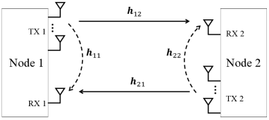
Figure 1: The MISO point-to-point full-duplex network under study. The solid line denotes the desired channel and the dashed line denotes the self-interference channel.

In this paper, we consider the optimal signaling structure for the MISO full-duplex two-way channel, by which all rate pairs on the boundary of the achievable rate region can be achieved. We introduce the channel model that includes transmit front-end noise. We leverage our model to characterize the achievable rate region for the full-duplex channel. The boundary of the region is described by a family of non-convex optimization problems. Rendering the computation tractable, we decouple the original non-convex problems to the family of convex optimization problems. The decoupling method was first developed in the field of game theory [8] and recently introduced to communications in [9, 10, 11, 12, 13]. By employing the semi-definite programing (SDP) reformulation, we numerically solve the optimal signaling and prove the optimality of transmit beamforming. That is to say, for a MISO full-duplex two-way channel, all the points on the boundary of the achievable rate region can be achieved by restricting to transmit beamforming scheme. Furthermore, we derive the closed-form optimal beamforming weights. Finally, through simulations we show the achievable rate regions for the MISO full-duplex two-way channels and evaluate the performance of the traditional zero-forcing beamforming with our optimal beamforming.

Notation: We use $(\cdot)^{{\dagger}}$ to denote conjugate transpose. For a scalar $a$, we use $|a|$ to denote the absolute value of $a$. For a vector $\boldsymbol{a}\in\mathbb{C}^{M\times 1}$, we use $\|\boldsymbol{a}\|$ to denote the norm, $\boldsymbol{a}^{(k)}$ to denote the $k^{th}$ element of $\boldsymbol{a}$, $\text{Diag}(\boldsymbol{a})$ to denote the square diagonal matrix with the elements of vector $\boldsymbol{a}$ on the main diagonal. For a matrix $\boldsymbol{A}\in\mathbb{C}^{M\times M}$, we use $\boldsymbol{A}^{-1}$, $\textbf{tr}(\boldsymbol{A})$ and $\text{rank}(\boldsymbol{A})$ to denote the inverse, the trace and the rank of $\boldsymbol{A}$, respectively. We use $\text{diag}(\boldsymbol{A})$ to denote the diagonal matrix with the same diagonal elements as $\boldsymbol{A}$. $\boldsymbol{A}\succeq 0$ means that $\boldsymbol{A}$ is a positive semidefinite Hermitian matrix. We denote expectation, variance and covariance by $\text{E}\{\cdot\}$, $\text{Var}\{\cdot\}$ and $\text{Cov}\{\cdot\}$, respectively. Finally, $\mathbb{C}$ and $\mathbb{H}$ denotes the complex field and the Hermitian symmetric space, respectively.

II Channel Model

We present the channel model for a MISO full-duplex network with two nodes as illustrated in Fig. 1. Assume two nodes indexed by $i,j\in\{1,2\}$ share the same single frequency band for transmission. Each node is equipped with $M$ transmit antennas and a single receive antenna. The signal from transmitter $i$ is collected as the signal of interest by receiver $j,j\neq i$, while appears at its own receiver $i$ as the self-interference signal.

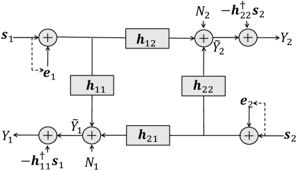
Figure 2: The model of the MISO full-duplex two-way channel under study.

Fig. 2 summarizes our model of the MISO full-duplex two-way channel. Denote the wireless channel from transmitter $i$ to receiver $j$ by the complex vector $\boldsymbol{h}_{ij}\in\mathbb{C}^{M\times 1}$. The signal at receiver $i$ is given by

$$\widetilde{Y}_{i}=\boldsymbol{h}_{ji}^{{\dagger}}(\boldsymbol{s}_{j}+\boldsymbol{e}_{j})+\boldsymbol{h}_{ii}^{{\dagger}}(\boldsymbol{s}_{i}+\boldsymbol{e}_{i})+N_{i}$$ (1)

where $\boldsymbol{s}_{i}\in\mathbb{C}^{M\times 1}$ denotes the transmit signal prior to the transmit front-end chain at transmitter $i$. An additional transmit front-end noise $\boldsymbol{e}_{i}$ is propagated over the same channel as $\boldsymbol{s}_{i}$. At receiver $i$, the thermal noise is modeled as a complex Gaussian noise $N_{i}\sim\mathcal{CN}(0,\sigma_{N}^{2})$.

The transmit front-end noise $\boldsymbol{e}_{i}$ is induced by the imperfect transmit front-end chain [4, 5]. More precisely $\boldsymbol{e}_{i}$ statistically relates to the transmit signal $\boldsymbol{s}_{i}$ due to the limited dynamic range of the transmit front-end chain [4, 6]. Denote the covariance of $\boldsymbol{s}_{i}$ by $\boldsymbol{Q}_{i}\triangleq\text{Cov}\{\boldsymbol{s}_{i}\}$. Note that the diagonal elements of $\boldsymbol{Q}_{i}$ represent the transmit signal power. Following the results in [14, 6, 15], we model $\boldsymbol{e}_{i}$ as the independent Gaussian vector with zero mean and covariance $\text{Cov}\{\boldsymbol{e}_{i}\}=\beta\text{diag}(\boldsymbol{Q}_{i})$ where $\beta$ is a constant depending on the distortion level of the transmit front-end chain [1].

At receiver $i$, the signal of interest $\boldsymbol{h}_{ji}^{{\dagger}}\boldsymbol{s}_{j},j\neq i$ is received along with the self-interference signal $\boldsymbol{h}_{ii}^{{\dagger}}\boldsymbol{s}_{i}$ and the transmit front-end noise $\boldsymbol{h}_{ji}^{{\dagger}}\boldsymbol{e}_{j}$, $\boldsymbol{h}_{ii}^{{\dagger}}\boldsymbol{e}_{i}$. The power level of $\boldsymbol{h}_{ji}^{{\dagger}}\boldsymbol{e}_{j},j\neq i$ is typically much lower than that of the thermal noise $N_{i}$ and thus can be neglected[5]. However, $\boldsymbol{h}_{ii}^{{\dagger}}\boldsymbol{e}_{i}$ is in the power level close to the signal of interest and needs to be considered for the analysis, since the gain of the self-interference channel $\boldsymbol{h}_{ii}$ may be $100$dB higher than the gain of the cross-node channel $\boldsymbol{h}_{ji}$ [6]. In addition to the strength, transmitters and receivers on a same node are relatively static, resulting in long coherence time of self-interference channels, thus receiver $i$ is assumed to have the perfect knowledge of its own self-interference channel $\boldsymbol{h}_{ii}$ [5]. Note that receiver $i$ also knows its own transmitted signal $\boldsymbol{s}_{i}$. Then we can eliminate the self-interference $\boldsymbol{h}_{ii}^{{\dagger}}\boldsymbol{s}_{i}$ before decoding. The signal after cancellation is given by

$$Y_{i}=\boldsymbol{h}_{ji}^{{\dagger}}\boldsymbol{s}_{j}+\boldsymbol{h}_{ii}^{{\dagger}}\boldsymbol{e}_{i}+N_{i}$$ (2)

where $\boldsymbol{h}_{ii}^{{\dagger}}\boldsymbol{e}_{i}$ represents the residual self-interference. By defining the aggregate noise term $V_{i}\triangleq\boldsymbol{h}_{ii}^{{\dagger}}\boldsymbol{e}_{i}+N_{i}$, the received signal model can be further simplified as

$$\begin{split}Y_{i}=\boldsymbol{h}_{ji}^{{\dagger}}\boldsymbol{s}_{j}+V_{i}\\ \end{split}$$ (3)

where $V_{i}$ is Gaussian noise with zero mean and variance $\text{Var}\{V_{i}\}=\sigma_{N}^{2}+\beta\boldsymbol{h}_{ii}^{{\dagger}}\text{diag}(\boldsymbol{Q}_{i})\boldsymbol{h}_{ii}$.

III Boundary of Achievable Rate Region

We present the achievable rate region for the MISO full-duplex two-way channel and characterize the boundary points of this region by a family of coupled nonconvex optimization problems. Next, we show that the boundary points can be alternatively obtained by solving a family of convex optimization problems that are the results of the transformation of the original nonconvex optimization problems.

III-A Achievable Rate Region and Pareto Boundary

As shown in (3), the channel model for the wireless link from node $2$ to node $1$ is equivalent to a Gaussian channel. It follows from the results of [16, 17] that by employing a Gaussian codebook at node $2$, we can achieve the maximum rate for the channel from node $2$ to node $1$

$$R_{1}(\boldsymbol{Q}_{1},\boldsymbol{Q}_{2})=\log\Bigg{(}1+\frac{\boldsymbol{h}_{21}^{{\dagger}}\boldsymbol{Q}_{2}\boldsymbol{h}_{21}}{\sigma_{N}^{2}+\beta\boldsymbol{h}_{11}^{{\dagger}}\text{diag}(\boldsymbol{Q}_{1})\boldsymbol{h}_{11}}\Bigg{)}$$ (4)

where $(\boldsymbol{Q}_{1},\boldsymbol{Q}_{2})$ are the given transmit covariance matrices. Similarly, the maximum rate for the channel from node $1$ to node $2$ is equal to

$$R_{2}(\boldsymbol{Q}_{1},\boldsymbol{Q}_{2})=\log\Bigg{(}1+\frac{\boldsymbol{h}_{12}^{{\dagger}}\boldsymbol{Q}_{1}\boldsymbol{h}_{12}}{\sigma_{N}^{2}+\beta\boldsymbol{h}_{22}^{{\dagger}}\text{diag}(\boldsymbol{Q}_{2})\boldsymbol{h}_{22}}\Bigg{)}.$$ (5)

Any rate pair $(r_{1},r_{2})$ with $r_{1}\leq R_{1},r_{2}\leq R_{2}$, is achievable for the MISO full-duplex two-way channel.

Define the achievable rate region for the MISO full-duplex two-way channel to be the set of all achievable rate pairs under the transmit power constraint $P_{i}$:

$$\mathcal{R}\triangleq\bigcup_{\scriptstyle\textbf{tr}(\boldsymbol{Q}_{i})\leq P_{i},\atop\scriptstyle\boldsymbol{Q}_{i}\succeq 0,i=1,2}\left\{\begin{split}&(r_{1},r_{2}):\\ &0\leq r_{1}\leq R_{1}(\boldsymbol{Q}_{1},\boldsymbol{Q}_{2})\\ &0\leq r_{2}\leq R_{2}(\boldsymbol{Q}_{1},\boldsymbol{Q}_{2})\end{split}\right\}.$$ (6)

A rate pair is on the boundary of the rate region $\mathcal{R}$ if and only if it is Pareto optimal which is defined as follows (A similar definition can be found in [18, 12, 13]).

Definition 1: (Pareto optimality) A rate pair $(R_{1}^{*},R_{2}^{*})\in\mathcal{R}$ is Pareto optimal if there does not exist another rate pair $(R_{1},R_{2})\in\mathcal{R}$ such that $(R_{1},R_{2})\geq(R_{1}^{*},R_{2}^{*})$ and $(R_{1},R_{2})\neq(R_{1}^{*},R_{2}^{*})$ where the inequality is component-wise.

Accordingly, the set of all boundary points of the achievable rate region $\mathcal{R}$ is called Pareto boundary and defined as

$$\mathcal{R}^{*}=\bigcup\;\{\text{all the Pareto optimal rate pairs}\;\;(R_{1}^{*},R_{2}^{*})\}.$$ (7)

It is shown in [9, 10] that $\mathcal{R}^{*}$ can be derived by solving a family of nonconvex optimization problems:

$$\begin{split}\max\;\;&{\mu_{1}R_{1}(\boldsymbol{Q}_{1},\boldsymbol{Q}_{2})+\mu_{2}R_{2}(\boldsymbol{Q}_{1},\boldsymbol{Q}_{2})}\\ \text{subject to}\;\;&\textbf{tr}(\boldsymbol{Q}_{i})\leq P_{i},\boldsymbol{Q}_{i}\succeq 0,i=1,2\end{split}$$ (8)

where $0\leq\mu_{1}<\infty$ and $0\leq\mu_{2}<\infty$. However, the non-convexity of problem (8) implies that we must go through all possible transmit covariance matrices $\boldsymbol{Q}_{1}$ and $\boldsymbol{Q}_{2}$ to find the optimal solution for each $(\mu_{1},\mu_{2})$ pair. What is worse, the complexity of such exhaustive search exponentially increases with the dimensions of $\boldsymbol{Q}_{1}$ and $\boldsymbol{Q}_{2}$, which renders the computation intractable [10]. Next, we present an alternative approach more suitable for deriving the Pareto boundary for the MISO full-duplex two-way channel.

III-B Decoupled Optimization Problems

The difficulty in deriving Pareto boundary $\mathcal{R}^{*}$ is caused by the non-convexity and the coupled high-dimensional nature of problem (8). To reduce the computationally complexity, we need to decouple problem (8) in terms of lower-dimensional variables. Using the decoupling procedure in [9, 10, 13] we introduce an auxiliary variable $z_{i}$ for node $i$ which denotes the power of the signal of interest at node $j$ i.e., $z_{i}\triangleq{\boldsymbol{h}_{ij}^{{\dagger}}\boldsymbol{Q}_{i}\boldsymbol{h}_{ij}}$. Consider the following optimization problem for node $i$ with the transmit power constraint $P_{i}$:

$$\begin{split}\min\;\;&{\boldsymbol{h}_{ii}^{{\dagger}}\text{diag}(\boldsymbol{Q}_{i})\boldsymbol{h}_{ii}}\\ \text{subject to}\;\;&{\boldsymbol{h}_{ij}^{{\dagger}}\boldsymbol{Q}_{i}\boldsymbol{h}_{ij}}=z_{i}\\ &\textbf{tr}(\boldsymbol{Q}_{i})\leq P_{i},\boldsymbol{Q}_{i}\succeq 0\end{split}$$ (9)

where $i,j\in\{1,2\}$ and $i\neq j$. We require

$$0\leq z_{i}\leq\max\limits_{\textbf{tr}(\boldsymbol{Q}_{i})\leq P_{i},\boldsymbol{Q}_{i}\succeq 0}\boldsymbol{h}_{ij}^{{\dagger}}\boldsymbol{Q}_{i}\boldsymbol{h}_{ij}=P_{i}\|\boldsymbol{h}_{ij}\|^{2}$$ (10)

so that problem (9) always has a feasible solution. Denote the optimal value of problem (9) as $\Gamma_{i}^{*}(z_{i})$. Then, we define a set in terms of $z_{i}$ and $\Gamma_{i}^{*}(z_{i})$ as follows:

$$\overline{\mathcal{R}}\triangleq\bigcup_{\scriptstyle z_{1}\in[0,P_{1}\|\boldsymbol{h}_{12}\|^{2}],\atop\scriptstyle z_{2}\in[0,P_{2}\|\boldsymbol{h}_{21}\|^{2}]}\left\{\begin{split}&(r_{1},r_{2}):\\ &r_{1}=\log\Bigg{(}1+\frac{z_{2}}{\sigma_{N}^{2}+\beta\Gamma_{1}^{*}(z_{1})}\Bigg{)}\\ &r_{2}=\log\Bigg{(}1+\frac{z_{1}}{\sigma_{N}^{2}+\beta\Gamma^{*}_{2}(z_{2})}\Bigg{)}\end{split}\right\}.$$

Any rate pair in the above set $\overline{\mathcal{R}}$ can be achieved by the optimal solution $\boldsymbol{Q}_{1}^{*}$ and $\boldsymbol{Q}_{2}^{*}$ for problem (9) with some $z_{1}$ and $z_{2}$, thus $\overline{\mathcal{R}}$ is a subset of the achievable rate region $\mathcal{R}$ in (6). In Lemma 1 we show that $\overline{\mathcal{R}}$ includes the Pareto boundary $\mathcal{R}^{*}$ for the region $\mathcal{R}$.

Lemma 1: Under the transmit power constraint $P_{i}$, any point on the Pareto boundary $\mathcal{R}^{*}$ for the achievable rate region $\mathcal{R}$ in (6) can be achieved by the optimal solution $\boldsymbol{Q}_{i}^{*}$ for problem (9) with some $z_{i}$. That is to say, $\mathcal{R}^{*}\subseteq\overline{\mathcal{R}}$.

Proof:

For any point $(R_{1}^{*},R_{2}^{*})$ on the Pareto boundary, assume that it is achieved by $\boldsymbol{Q}_{1}^{*}$ and $\boldsymbol{Q}_{2}^{*}$. $\boldsymbol{Q}_{i}^{*}$ is a feasible solution for problem (9) with $z_{i}=z_{i}^{*}=\boldsymbol{h}_{ij}^{{\dagger}}\boldsymbol{Q}_{i}^{*}\boldsymbol{h}_{ij}$ where $i,j\in\{1,2\}$ and $i\neq j$. Let $i=1$, if $\boldsymbol{Q}_{1}^{*}$ is not an optimal solution for problem (9) i.e., $\boldsymbol{h}_{11}^{{\dagger}}\text{diag}(\boldsymbol{Q}_{1}^{*})\boldsymbol{h}_{11}>\Gamma_{1}^{*}(z_{1}^{*})$ then

$$R_{1}^{*}<\log\Bigg{(}1+\frac{z_{2}^{*}}{\sigma_{N}^{2}+\beta\Gamma_{1}^{*}(z_{1}^{*})}\Bigg{)}=\overline{R_{1}},$$

while

$$R_{2}^{*}\leq\log\Bigg{(}1+\frac{z_{1}^{*}}{\sigma_{N}^{2}+\beta\Gamma_{2}^{*}(z_{2}^{*})}\Bigg{)}=\overline{R_{2}}.$$

As $(\overline{R_{1}},\overline{R_{2}})$ belongs to $\overline{\mathcal{R}}$ and thus belongs to $\mathcal{R}$, $R_{1}^{*}<\overline{R_{1}}$ and $R_{2}^{*}\leq\overline{R_{2}}$ contradict to the Pareto optimality of $(R_{1}^{*},R_{2}^{*})$. Therefore $\boldsymbol{Q}_{1}^{*}$ is an optimal solution for problem (9). In the same way we can show that $\boldsymbol{Q}_{2}^{*}$ is an optimal solution for problem (9). ∎

We stress that the set $\overline{\mathcal{R}}$ is not necessarily equivalent to the Pareto boundary $\mathcal{R}^{*}$, since $\overline{\mathcal{R}}$ may include the rate pairs inside the region $\mathcal{R}$. However, the relationship $\mathcal{R}^{*}\subseteq\overline{\mathcal{R}}$ implies that any approach of obtaining the set $\overline{\mathcal{R}}$ will suffice to derive the entire Pareto boundary $\mathcal{R}^{*}$. Furthermore, any result applying to $\overline{\mathcal{R}}$ also works for $\mathcal{R}^{*}$. Hence, we proceed to explore the optimal signaling for the MISO full-duplex two-way channel by the study of the set $\overline{\mathcal{R}}$.

IV Optimal Signaling

By solving problem (9), we show the optimality of transmit beamforming for the MISO full-duplex two-way channel. In other words, all the points on the Pareto boundary $\mathcal{R}^{*}$ of the achievable rate region $\mathcal{R}$ can be achieved by transmit beamforming. To better understand the optimal signaling, we provide the closed form of the optimal beamforming weights.

IV-A Semidefinite Programming Reformulation

Problem (9) is not a common optimization problem since the objective function includes the non-linear operator $\text{diag}(\cdot)$. By setting $\boldsymbol{A}_{i}=\boldsymbol{h}_{ij}\boldsymbol{h}_{ij}^{\dagger}$, $\boldsymbol{C}_{i}=\text{Diag}(|\boldsymbol{h}_{ii}^{(1)}|^{2},\dots,|\boldsymbol{h}_{ii}^{(M)}|^{2})$ and using the equivalent relationship $\boldsymbol{h}_{ii}^{{\dagger}}\text{diag}(\boldsymbol{Q}_{i})\boldsymbol{h}_{ii}=\textbf{tr}(\boldsymbol{C}_{i}\boldsymbol{Q}_{i})$, we reformulate problem (9) to the semi-definite programming (SDP) problem as follows (See more details about SDP in [19]):

$$\begin{split}\min\;\;&{\textbf{tr}(\boldsymbol{C}_{i}\boldsymbol{Q}_{i})}\\ \text{subject to}\;\;&\textbf{tr}(\boldsymbol{A}_{i}\boldsymbol{Q}_{i})=z_{i},\\ &\textbf{tr}(\boldsymbol{Q}_{i})\leq P_{i},\boldsymbol{Q}_{i}\succeq 0\\ \end{split}$$ (11)

where $\boldsymbol{C}_{i},\boldsymbol{A}_{i}\in\mathbb{H}^{M}$.

The above SDP reformulation reveals the hidden convexity of problem (9) so that we can solve it by employing the well-developed interior-point algorithm within polynomial time. Furthermore, we can numerically characterize the Pareto boundary for the MISO full-duplex two-way channel in efficiency.

IV-B Optimal Beamforming

The optimal solutions for problem (11) determine the signaling structure to achieve the rate pairs in the set $\overline{\mathcal{R}}$. In Theorem 1, we explore the rank of optimal solutions $\boldsymbol{Q}^{*}_{i}$ for problem (11) where $i,j\in\{1,2\}$ and $i\neq j$.

Theorem 1: For problem (11) with $P_{i}\geq 0$ and $0\leq z_{i}\leq P_{i}\|\boldsymbol{h}_{ij}\|^{2}$, there always exists an optimal solution $\boldsymbol{Q}_{i}^{*}$ with $\text{rank}(\boldsymbol{Q}^{*}_{i})=1$.

Proof:

See the Appendix. ∎

Note that the transmit signal with the rank-one covariance matrix can be implemented by transmitter beamforming. It follows from Theorem 1 that all points in the set $\overline{\mathcal{R}}$, which include the entire Pareto boundary, can be achieved by the transmitter beamforming. Therefore, we conclude that transmitter beamforming is an optimal scheme for the MISO full-duplex two-way channel. In Lemma 2 we derive the closed-form optimal weights for transmitter beamforming.

Lemma 2: For node $i$ in the MISO point-to point full-duplex wireless network with the transmit power constraint $P_{i}$ and complex channels $\boldsymbol{h}_{ii},\boldsymbol{h}_{ij},i,j\in\{1,2\},i\neq j$, the optimal beamforming weights have the following form:

$$\boldsymbol{w}_{i}^{*}=\frac{\sqrt{z_{i}}(\boldsymbol{C}_{i}+\epsilon\boldsymbol{I})^{-1}\boldsymbol{h}_{ij}}{\boldsymbol{h}_{ij}^{\dagger}(\boldsymbol{C}_{i}+\epsilon\boldsymbol{I})^{-1}\boldsymbol{h}_{ij}}$$ (12)

where $\boldsymbol{C}_{i}=\text{Diag}(|\boldsymbol{h}_{ii}^{(1)}|^{2},\dots,|\boldsymbol{h}_{ii}^{(M)}|^{2})$, constant $z_{i}$ is within the range $0\leq z_{i}\leq P_{i}\|\boldsymbol{h}_{ij}\|^{2}$ and $\boldsymbol{I}$ denotes the $M\times M$ identical matrix. For a fixed $z_{i}$, nonnegative constant $\epsilon$ is adjusted to satisfy the transmit power constraint $\|\boldsymbol{w}_{i}\|^{2}\leq P_{i}$. Specially, $\epsilon=0$ if

$$z_{i}\leq\frac{P_{i}(\boldsymbol{h}_{ij}^{{\dagger}}\boldsymbol{C}_{i}^{-1}\boldsymbol{h}_{ij})^{2}}{\boldsymbol{h}_{ij}^{{\dagger}}\boldsymbol{C}_{i}^{-2}\boldsymbol{h}_{ij}}.$$ (13)

Proof:

The optimal beamforming weights can be obtained by solving problem (11) with the rank-one constraint $\boldsymbol{Q}_{i}=\boldsymbol{w}_{i}\boldsymbol{w}_{i}^{{\dagger}}$ as follows:

$$\begin{split}\min\;\;&{\boldsymbol{w}_{i}^{{\dagger}}\boldsymbol{C}_{i}\boldsymbol{w}_{i}}\\ \text{subject to}\;\;&|\boldsymbol{w}_{i}^{{\dagger}}\boldsymbol{h}_{ij}|^{2}=z_{i},\|\boldsymbol{w}_{i}\|^{2}\leq P_{i}.\end{split}$$ (14)

The above problem has the general closed-form optimal solution (12) (see details in [20]). Without the transmit power constraint $\|\boldsymbol{w}_{i}\|^{2}\leq P_{i}$, problem (14) has the following optimal solution (shown in [20])

$$\boldsymbol{w}_{i}^{*}=\frac{\sqrt{z_{i}}\boldsymbol{C}_{i}^{-1}\boldsymbol{h}_{ij}}{\boldsymbol{h}_{ij}^{\dagger}\boldsymbol{C}_{i}^{-1}\boldsymbol{h}_{ij}}.$$

Combining with the condition (13), we obtain

$$\|\boldsymbol{w}_{i}^{*}\|^{2}=\frac{z_{i}\boldsymbol{h}_{ij}^{{\dagger}}\boldsymbol{C}_{i}^{-2}\boldsymbol{h}_{ij}}{(\boldsymbol{h}_{ij}^{{\dagger}}\boldsymbol{C}_{i}^{-1}\boldsymbol{h}_{ij})^{2}}\leq P_{i}.$$

Hence, we conclude that $\epsilon=0$ under the condition (13). ∎

We remark that the optimal beamforming weights for node $i$ are closely parallel to the cross-node channel $\boldsymbol{h}_{ij}$, beamforming the signal of interest at node $j$. While the transmit front-end noise corresponding to the stronger self-interference channel is largely suppressed via the matrix $(\boldsymbol{C}_{i}+\epsilon\boldsymbol{I})^{-1}$.

V Numerical Examples

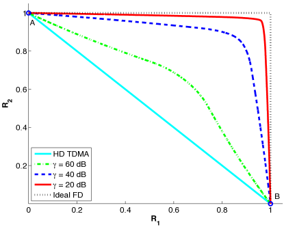
Figure 3: The achievable rate regions for the symmetric MISO full-duplex two-way channels with $\beta=-40\;\text{dB}$, $\|\boldsymbol{h}_{12}\|=\|\boldsymbol{h}_{21}\|=1$, $P_{1}=P_{2}=1$. As plotted for comparison is the half-duplex TDMA achievable rate region.

We present the achievable rate regions for the MISO full-duplex two-way channels in Fig. 3 where the channels are symmetric i.e., $\boldsymbol{h}_{12}=\boldsymbol{h}_{21}$ and $\boldsymbol{h}_{11}=\boldsymbol{h}_{22}$. Each node is equipped with $M=3$ transmit antennas and single receive antenna with the transmit power constraints $P_{1}=P_{2}$ and the receiver noise $\sigma_{N}^{2}=1$. Define $\gamma=\frac{\|\boldsymbol{h}_{11}\|}{\|\boldsymbol{h}_{21}\|}=\frac{\|\boldsymbol{h}_{22}\|}{\|\boldsymbol{h}_{12}\|}$ (in dB) to represent the ratio of the self-interference channel gain to the cross-node channel gain. Note that $\gamma$ can be reduced by the passive suppression [3]. The transmit front-end noise level is fixed with $\beta=-40$dB. Each colored line represents the Pareto boundary of the achievable rate region for the channel with corresponding $\gamma$. We conclude from the numerical results that the achievable rate region shrinks as $\gamma$ varies from $20$dB to $60$dB. However, the full-duplex channel always outperforms than the half-duplex TDMA channel if the optimal beamforming is employed. The extreme points $A,B$ of the rate regions on the axes represent the maximum rates in the case that only one-way of the two-way channel is working. It follows that the points $A,B$ are only determined by the transmit power constraints $P_{i}$. The ideal MISO full-duplex two-way channel sets the outer bound for the achievable rate regions of all channels, doubling that of the half-duplex TDMA channel.

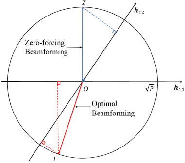
Figure 4: The geometric comparison of the full-duplex optimal beamforming with the zero-forcing beamforming

The rate pair with the maximum sum-rate corresponds to the point with $R_{1}=R_{2}$ on the Pareto boundary and can be achieved by certain weights in the set of optimal beamforming weights defined in Lemma 2. In Fig. 4 we compare the optimal weights $\overline{OF}$ which corresponds to the maximum sum-rate with the zero-forcing (ZF) beamforming weights $\overline{OZ}$. For simplicity, we assume all channel vectors to be $2\times 1$ real vectors with $\boldsymbol{h}_{11}=\boldsymbol{h}_{22}$ and $\boldsymbol{h}_{12}=\boldsymbol{h}_{21}$. Assume the transmit power constraints $P_{1}=P_{2}=P$. Then all possible beamforming weights are contained in the disc with radius $\sqrt{P}$. $\overline{OZ}$ restricts the transmit signal orthogonal to the self-interference channel $\boldsymbol{h}_{ii}$, whereas $\overline{OF}$ is not orthogonal to $\boldsymbol{h}_{ii}$ but has greater length of projection on the cross-node channel $\boldsymbol{h}_{ij}$.

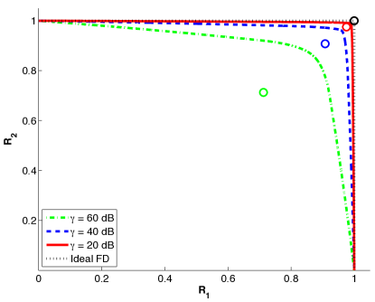
Figure 5: The achievable rate regions for the symmetric MISO two-way full-duplex channel with $\beta=-60\;\text{dB}$. Circles denote the respective ZF beamforming rates for $\gamma=20\;\text{dB},\gamma=40\;\text{dB},\gamma=60\;\text{dB}$ and the ideal full-duplex network.

In Fig. 5, we evaluate the performance of the ZF beamforming for the same full-duplex channels as in Fig. 3 but with $\beta=-60$ dB. Comparing the channel with the same $\gamma$ in Fig. 3 and Fig. 5, the achievable rate region is increased due to reduction of $\beta$. The circles, which represent the rate pairs achieved by the ZF beamforming, are below the corresponding Pareto boundaries except for the ideal full-duplex channel. It follows that the ZF beamforming is not optimal for the MISO full-duplex channel in presence of the residual self-interference. As shown in Fig. 4, the ZF beamforming generates no interference at the unintended receiver if the interference equals to the projection of the transmit signal on the interference channel. However, for the full-duplex case in (2), the residual self-interference signal statistically depends on the transmit signal power rather than being the projection of the transmit signal on $\boldsymbol{h}_{ii}$. Therefore, the ZF beamforming is inefficient in the suppression of the residual self-interference. With $\gamma$ decreasing, the residual self-interference signal is gradually weaker and thus the ZF beamforming is closer to the optimal beamforming and is exactly optimal in the ideal full-duplex network.

VI Conclusion

We considered the MISO point-to-point full-duplex wireless network. We derived the achievable rate region and the characterization of the Pareto boundary for the MISO two-way full-duplex channel in presence of the transmit front-end noise. Using the decoupling technique and SDP reformulation, we proposed a new method to obtain the entire Pareto boundary by solving a family of convex SDP problems, rather than the original non-convex problems. We showed that any rate pair on the Pareto boundary can be achieved by the beamforming transmission strategy. Finally, we provided the closed-form solution for the optimal beamforming weights of the MISO full-duplex two-way channel.

Appendix

Proof of Theorem 1: We prove Theorem 1 by the primal-dual method. Note that problem (11) is feasible and bounded. It follows that its dual problem is also feasible and bounded [19]. Assume $\boldsymbol{Q}^{*}$ is an optimal solution for problem (11). From [19], problem (11) has the dual problem as follows:

$$\begin{split}\min_{\lambda_{1},\lambda_{2}}\;\;&{\lambda_{1}z_{i}+\lambda_{2}P}\\ \hskip 20.0pt\text{subject to}\;\;&\boldsymbol{Z}=\boldsymbol{C}_{i}-{\lambda_{1}\boldsymbol{A}_{i}}-{\lambda_{2}\boldsymbol{I}}\succeq 0.\\ \end{split}$$ (15)

where $P=\textbf{tr}(\boldsymbol{Q}^{*})$. Assume $((\lambda_{1}^{*},\lambda_{2}^{*}),\boldsymbol{Z}^{*})$ are the optimal solutions for (15). We denote the rank of $\boldsymbol{Q}^{*}$ by $r$. We assume $r>1$. Following that $\boldsymbol{Q}^{*}$ is positive semi-definite, $\boldsymbol{Q}^{*}$ can then be written as $\boldsymbol{Q}^{*}=\boldsymbol{V}\boldsymbol{V}^{{\dagger}}$ via the singular-value decomposition where $\boldsymbol{V}\in\mathbb{C}^{M\times r}$.

Next, we consider the following two linear equations defined by $\boldsymbol{A}_{i}$ and $\boldsymbol{V}$:

$$\left\{\begin{split}&\textbf{tr}(\boldsymbol{V}^{{\dagger}}\boldsymbol{A}_{i}\boldsymbol{V}\boldsymbol{X})=0\\ &\textbf{tr}(\boldsymbol{V}^{{\dagger}}\boldsymbol{V}\boldsymbol{X})=0\\ \end{split}\right.$$ (16)

where the unknown matrix $\boldsymbol{X}\in\mathbb{H}^{r}$ contains $r^{2}$ real-valued unknowns, that is, $\frac{r(r+1)}{2}$ for the real part and $\frac{r(r-1)}{2}$ for the imaginary part.

The linear system (16) must have a non-zero solution, denoted by $\boldsymbol{X}^{*}$, since it has $r^{2}$ unknowns where $r\geq 2$. By decomposing the Hermitian matrix ${\boldsymbol{X}^{*}}$, we obtain ${\boldsymbol{X}^{*}}=\boldsymbol{U}\boldsymbol{\Sigma}\boldsymbol{U}^{{\dagger}}$, where $\boldsymbol{U}$ is an $r$ dimensional unitary matrix and $\boldsymbol{\Sigma}$ is the diagonal matrix, $\boldsymbol{\Sigma}=\text{Diag}(\sigma_{1},\dots,\sigma_{r})$. Without loss of generality, we assume $|\sigma_{1}|\geq|\sigma_{2}|\dots\geq|\sigma_{r}|$. Non-zero matrix $\boldsymbol{X}^{*}$ has at least one non-trivial eigenvalue, thus $|\sigma_{1}|>0$. Next, we construct a new matrix as follows:

$${\boldsymbol{Q}^{*}_{(1)}}=\boldsymbol{V}(\boldsymbol{I}-\frac{1}{\sigma_{1}}{\boldsymbol{X}^{*}})\boldsymbol{V}^{{\dagger}}.$$ (17)

Note that $\boldsymbol{I}-\frac{1}{\sigma_{1}}{\boldsymbol{X}^{*}}\succeq 0$. It follows that $\boldsymbol{Q}^{*}_{(1)}$ is positive semi-definite. Next, we show that $\boldsymbol{Q}^{*}_{(1)}$ is also an optimal solution for problem (11). Note that $\boldsymbol{Q}^{*}_{(1)}$ is optimal for problem (11) if and only if $(\boldsymbol{Q}^{*}_{(1)},(\lambda_{1}^{*},\lambda_{2}^{*}),\boldsymbol{Z}^{*})$ satisfies the KKT conditions, including the primal feasibility, the dual feasibility and the complementarity [21]. As $((\lambda_{1}^{*},\lambda_{2}^{*}),\boldsymbol{Z}^{*})$ is unchanged, the dual feasibility is automatically satisfied. Therefore, we need only to prove the primal feasibility and the complementarity of $\boldsymbol{Q}^{*}_{(1)}$.

$\boldsymbol{Q}^{*}_{(1)}$ is a feasible solution for problem (11), since the following two equations hold for $\boldsymbol{Q}^{*}_{(1)}$,

$$\begin{split}\textbf{tr}(\boldsymbol{A}_{i}\boldsymbol{Q}^{*}_{(1)})&=\textbf{tr}(\boldsymbol{A}_{i}\boldsymbol{V}(\boldsymbol{I}-\frac{1}{\sigma_{1}}{\boldsymbol{X}^{*}})\boldsymbol{V}^{{\dagger}})\\ &=\textbf{tr}(\boldsymbol{V}^{{\dagger}}\boldsymbol{A}_{i}\boldsymbol{V}\boldsymbol{I})-\frac{1}{\sigma_{1}}\textbf{tr}(\boldsymbol{V}^{{\dagger}}\boldsymbol{A}_{i}\boldsymbol{V}{\boldsymbol{X}^{*}})=z_{i},\end{split}$$

$$\begin{split}\textbf{tr}(\boldsymbol{Q}^{*}_{(1)})&=\textbf{tr}(\boldsymbol{V}(\boldsymbol{I}-\frac{1}{\sigma_{1}}{\boldsymbol{X}^{*}})\boldsymbol{V}^{{\dagger}})\\ &=\textbf{tr}(\boldsymbol{V}^{{\dagger}}\boldsymbol{V}\boldsymbol{I})-\frac{1}{\sigma_{1}}\textbf{tr}(\boldsymbol{V}^{{\dagger}}\boldsymbol{V}{\boldsymbol{X}^{*}})=P.\end{split}$$

To show the complementarity, note that $\textbf{tr}(\boldsymbol{Q}^{*}\boldsymbol{Z}^{*})=\textbf{tr}(\boldsymbol{V}^{{\dagger}}\boldsymbol{Z}^{*}\boldsymbol{V})=0$ and $\boldsymbol{V}^{{\dagger}}\boldsymbol{Z}^{*}\boldsymbol{V}\succeq 0$ implies that $\boldsymbol{V}^{{\dagger}}\boldsymbol{Z}^{*}\boldsymbol{V}=0$. It follows that

$$\textbf{tr}(\boldsymbol{Q}^{*}_{(1)}\boldsymbol{Z}^{*})=\textbf{tr}(\boldsymbol{V}(\boldsymbol{I}-\frac{1}{\sigma_{1}}{\boldsymbol{X}}^{*})\boldsymbol{V}^{{\dagger}}\boldsymbol{Z}^{*})\\ =\textbf{tr}((\boldsymbol{I}-\frac{1}{\sigma_{1}}{\boldsymbol{X}^{*}})\boldsymbol{V}^{{\dagger}}\boldsymbol{Z}^{*}\boldsymbol{V})=0.$$ (18)

Therefore, $\boldsymbol{Q}^{*}_{(1)}$ is an optimal solution for problem (11). Furthermore, the rank of $\boldsymbol{Q}^{*}_{(1)}$ is strictly smaller than $r$ since $\text{rank}(\boldsymbol{Q}^{*}_{(1)})=\text{rank}(\boldsymbol{I}-\frac{1}{\sigma_{1}}{\boldsymbol{X}^{*}})<r$.

We can repeat this process as $\boldsymbol{Q}^{*},\boldsymbol{Q}^{*}_{(1)},\boldsymbol{Q}^{*}_{(2)},\cdots$, until $\text{rank}(\boldsymbol{Q}^{*}_{(k)})\leq\sqrt{2}$. In other words, the rank of the optimal solution can be strictly decreasing to $\text{rank}(\boldsymbol{Q}^{*}_{(k)})\leq\sqrt{2}$, that is, $\text{rank}(\boldsymbol{Q}^{*}_{(k)})=1$.

References

- [1] A. Sahai, G. Patel, c. dick, and A. Sabharwal, “On the impact of phase noise on active cancelation in wireless full-duplex,” IEEE Trans. Vel. Technol., vol. 62, no. 9, pp. 4494–4510, Nov. 2013.
- [2] E. Everett, D. Dash, C. Dick, and A. Sabharwal, “Self-interference cancellation in multi-hop full-duplex networks via structured signaling,” in Proc. 49th Annu. Allerton Conf. Commun., Control, Comput., Monticello, IL, Sep. 2011, pp. 1619–1626.
- [3] E. Everett, M. Duarte, C. Dick, and A. Sabharwal, “Empowering full-duplex wireless communication by exploiting directional diversity,” in Proc. 45th Asilomar Conf. Signals, Syst., Comput., Pacific Grove, CA, Nov. 2011, pp. 2002–2006.
- [4] D. Bharadia, E. McMilin, and S. Katti, “Full duplex radios,” in Proc. ACM SIGCOMM. Hong Kong, China: ACM, 2013, pp. 375–386.
- [5] M. Vehkapera, T. Riihonen, and R. Wichman, “Asymptotic analysis of full-duplex bidirectional MIMO link with transmitter noise,” in IEEE Proc. 24th Int. Symp. Personal Indoor, Mobile Radio Commun. (PIMRC). IEEE, 2013, pp. 1265–1270.
- [6] B. Day, A. Margetts, D. Bliss, and P. Schniter, “Full-duplex bidirectional MIMO: Achievable rates under limited dynamic range,” IEEE Trans. Signal Process., vol. 60, no. 7, pp. 3702–3713, Jul. 2012.
- [7] M. Duarte, C. Dick, and A. Sabharwal, “Experiment-driven characterization of full-duplex wireless systems,” IEEE Trans. Wireless Commun., vol. 11, no. 12, pp. 4296–4307, Dec. 2012.
- [8] M. J. Osborne, An introduction to game theory, 1st ed. Cambridge, U.K.: Oxford University Press, 2004.
- [9] X. Shang and B. Chen, “Achievable rate region for downlink beamforming in the presence of interference,” in Proc. 41st Asilomar Conf. Signals, Syst., Comput., Nov. 2007, pp. 1684–1688.
- [10] X. Shang, B. Chen, and H. Poor, “Multiuser MISO interference channels with single-user detection: Optimality of beamforming and the achievable rate region,” IEEE Trans. Inf. Theory, vol. 57, no. 7, pp. 4255–4273, Jul. 2011.
- [11] E. Larsson and E. Jorswieck, “Competition versus cooperation on the MISO interference channel,” IEEE J. Sel. Areas Commun., vol. 26, no. 7, pp. 1059–1069, Sep. 2008.
- [12] E. A. Jorswieck, E. G. Larsson, and D. Danev, “Complete characterization of the pareto boundary for the MISO interference channel,” IEEE Trans. Signal Process., vol. 56, no. 10, pp. 5292–5296, 2008.
- [13] R. Zhang and S. Cui, “Cooperative interference management with MISO beamforming,” IEEE Trans. Signal Process., vol. 58, no. 10, pp. 5450–5458, 2010.
- [14] G. Santella and F. Mazzenga, “A hybrid analytical-simulation procedure for performance evaluation in m-qam-ofdm schemes in presence of nonlinear distortions,” IEEE Trans. Vel. Technol., vol. 47, no. 1, pp. 142–151, Feb. 1998.
- [15] H. Suzuki, T. V. A. Tran, I. Collings, G. Daniels, and M. Hedley, “Transmitter noise effect on the performance of a MIMO-OFDM hardware implementation achieving improved coverage,” IEEE J. Sel. Areas Commun., vol. 26, no. 6, pp. 867–876, Aug. 2008.
- [16] E. Telatar, “Capacity of multi-antenna gaussian channels,” European Trans. on Telecommun., vol. 10, no. 6, pp. 585–595, 1999.
- [17] T. M. Cover and J. A. Thomas, Elements of information theory, 2nd ed. Hoboken, NJ: John Wiley & Sons, 2006.
- [18] R. Mochaourab and E. Jorswieck, “Optimal beamforming in interference networks with perfect local channel information,” IEEE Trans. Signal Process., vol. 59, no. 3, pp. 1128–1141, Mar. 2011.
- [19] S. Boyd and L. Vandenberghe, Convex optimization. Cambridge, U.K.: Cambridge University Press, 2004.
- [20] H. Cox, R. M. Zeskind, and M. M. Owen, “Robust adaptive beamforming,” IEEE Trans. Acoust., Speech, Signal Process., vol. 35, no. 10, pp. 1365–1376, 1987.
- [21] Y. Huang and D. Palomar, “Rank-constrained separable semidefinite programming with applications to optimal beamforming,” IEEE Trans. Signal Process., vol. 58, no. 2, pp. 664–678, Feb. 2010.