Kondo dynamics in one-dimensional doped ferromagnetic insulators

Abstract

Some well-established examples of itinerant-electron ferromagnetism in one dimension occur in a Mott-insulating phase. We examine the consequences of doping a ferromagnetic insulator and coupling magnons to gapless charge fluctuations. Using a bosonization scheme for strongly interacting electrons, we derive an effective field theory for the magnon-holon interaction. When the magnon momentum matches the Fermi momentum of the holons, the backscattering of the magnon at low energies gives rise to a Kondo effect of a pseudospin defined from the chirality degree of freedom (right- or left-moving particles). The crossover between weak-coupling and strong-coupling fixed points of the effective mobile-impurity model is then investigated using a numerical renormalization group approach.

I Introduction

Ferromagnetism remains a challenging problem in physics, despite having been investigated ever since (and even before) the advent of quantum mechanics. It was Heisenberg who first realized that the phenomenon results from an interplay between electron-electron interactions and the Pauli exclusion principle: Heisenberg (1928) when two spin-polarized electrons occupy two orthogonal orbitals, their wave function must be spatially antisymmetric and vanishes when they occupy the same position. This leads to a lower expectation value of the Coulomb repulsion for electrons with the same spin. The dependence of energy levels on the relative spin orientation is often cast as an effective exchange interaction, which in this case is ferromagnetic as it favors parallel alignment of spins.

The mechanism of direct exchange can be generalized to the many-electron problem. However, its implications for the ground state are not so clear. On the one hand, mean-field arguments predict that a gas of itinerant electrons with local repulsive interactions will spontaneously break spin rotational symmetry and become ferromagnetic for sufficiently strong interaction. The precise condition for the transition is given by the Stoner criterion: $U\rho(E_{F})>1$, where $U$ is the interaction strength and $\rho(E_{F})$ is the density of states at the Fermi level. Fazekas (1999)

On the other hand, the Stoner criterion is not entirely reliable because the putative transition occurs in a nonperturbative regime of large $U$. Experimentally, the criterion remains controversial. In transition metal oxides, the existence of a ferromagnetic phase depends on detailed information about the band structure.Fazekas (1999) Recent observations in cold-atom systems have concluded first in favor of and later against an interaction-driven ferromagnetic transition. Jo et al. (2009); Sanner et al. (2012)

Itinerant ferromagnetism has proved hard to establish in microscopic models beyond mean-field approximations. For many years, explicit proofs relied on peculiar conditions such as the limit of vanishing hole doping Nagaoka (1966) or the presence of flat bands. Mielke (1991) In the domain of one-dimensional systems, there are even more constraints: a theorem due to Lieb and MattisLieb and Mattis (1962) rules out a ferromagnetic ground state for a number of models, including the paradigmatic Hubbard model.

The Lieb-Mattis theorem does not hold for models with hopping beyond nearest neighbors. In fact, TasakiTasaki (1995) proposed a two-band one-dimensional model whose ground state can be shown to be fully polarized for a wide range of hopping parameters and finite repulsion. Remarkably, the proof relies on the condition of quarter-filling, for which the model was conjectured to be a Mott insulator. One might then wonder whether ferromagnetic order survives in the metallic phase, reached by electron or hole doping. It is believed that it does, but the evidence relies mostly on variational methods and exact diagonalization for small chains.Penc et al. (1996); Fazekas (1999) There is stronger evidence based on density matrix renormalization group (DMRG) results for the single-band Hubbard model with next-nearest-neighbor hopping. Daul and Noack (1998) Only in the infinite-repulsion limit has metallic ferromagnetism been rigorously established, for a multi-band model with no flat bands.Tanaka and Tasaki (2007)

The nature of the ferromagnetic transition in one dimension has also been studied. Paramagnetic one-dimensional metals behave as Luttinger liquids, in which charge and spin excitations are described by two independent charge and spin bosonic fields. Haldane (1981) As the interaction increases and transition to a ferromagnetic phase supposedly occurs, the spin velocity must become negative. Daul and Noack (1998); Yang (2004); Wang et al. (2005) Theories have been proposed to describe second-order transitions for Ising Yang (2004); Bartosch et al. (2003) and $SU(2)$ Sengupta and Kim (2005) symmetries. First-order transitions are also a possibility. Nishimoto et al. (2008); Takayoshi et al. (2010)

In this work, we investigate the stability of doped Mott-insulating ferromagnets in one dimension at zero temperature by considering the creation of a magnon and its interaction with gapless charge fluctuations. This approach follows the spirit of current experiments designed to investigate phase transitions in cold atomic gases. Koschorreck et al. (2012); Fukuhara et al. (2013)

We organize our presentation as follows. Our starting point in Sec. II is a generalized version of the models proposed in Refs. Tasaki, 1995 and Penc et al., 1996. In the weakly interacting regime, we bosonize the model and show that the charge sector is a Mott insulator for quarter-filling while the Luttinger liquid in the spin sector remains stable. Section  III considers the model for the ferromagnetic phase in the strongly interacting regime. We use an alternative bosonization scheme Matveev et al. (2007); Akhanjee and Tserkovnyak (2007) to identify the spin and charge excitations in the large-$U$ limit as magnons and fermionic holons, respectively. In Sec. IV we analyze the low-doping limit of the metallic phase using an effective field theory with magnon-holon interactions dictated by symmetry considerations. A similar approach has been used to study magnons in a spinor Bose liquid. Kamenev and Glazman (2009) We find that, when the magnon momentum is commensurate with the holon Fermi surface, the scattering between opposite Fermi points gives rise to infrared singularities akin to the Kondo effect.Hewson (1997) This phenomenon has been previously discussed in the context of a mobile impurity in a Luttinger liquid.Lamacraft (2009); Schecter et al. (2012) In Sec. V, we proceed to studying the low-energy fixed points of our effective model using the numerical renormalization group.Krishna-murthy et al. (1980a); Bulla et al. (2008) Finally, Section VI summarizes our results.

II Weakly Interacting Regime

In Sec. I, we briefly mentioned Tasaki’s model, a one-dimensional model for which ferromagnetism has been rigorously established. Tasaki (1995) Tasaki’s Hamiltonian is

$$H=\sum_{i,j,\sigma}t_{ij}c^{\dagger}_{i,\sigma}c_{j,\sigma}+U\sum_{i}n_{i,\uparrow}n_{i,\downarrow},$$ (1)

where $c_{i,\sigma}$ is the annihilation operator for an electron with spin $\sigma=\uparrow,\downarrow$ at site $i$, $n_{i,\sigma}=c^{\dagger}_{i,\sigma}c^{\phantom{\dagger}}_{i,\sigma}$ is the number operator, $U\geq 0$ is the on-site repulsion, and the hopping amplitudes $t_{ij}$ are defined as follows:

$$t_{i,i+1} =t^{\prime}, \forall\,i,$$

$$t_{i,i+2} =t, \text{if $i$ is even},$$

$$t_{i,i+2} =-s, \text{if $i$ is odd},$$

$$t_{i,i} =V, \text{if $i$ is odd},$$

$$t_{i,j} =0,$$ otherwise.

Fig. 1 illustrates the Tasaki lattice. For $t\neq-s$, the lattice has two sites per unit cell. Tasaki demonstrated the existence of a ferromagnetic phase at quarter-filling when $t$ and $U$ are sufficiently large compared to $s$ and for the particular choices $V=0$ and $t^{\prime}=\sqrt{2}\left(t+s\right)$. Under these conditions, it can be shown that the expectation value of the Hamiltonian in an arbitrary state satisfies the inequality $\langle H\rangle\geq-2\left(s+t\right)N$, where $2N$ is the total number of sites. The lower bound happens to be precisely the energy of the fully polarized state, which proves that the latter is one of the ground states.Tasaki (1995) The ground state is $(2S_{tot}+1)$-fold degenerate, with $S_{tot}=N/2$ at quarter-filling, due to spontaneous symmetry breaking of the $SU(2)$ symmetry.

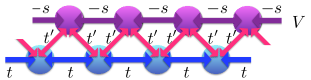
Figure 1: (color online) Tasaki’s one-dimensional model. The hopping between nearest neighbors is $t^{\prime}$. The hopping between next-nearest neighbors is $t$ ($-s$) for the even (odd) sublattice. The odd sublattice has chemical potential $V$. The on-site electronic repulsion in both sublattices is $U$.

Let us describe the low-energy excitations of Tasaki’s model, starting with the paramagnetic phase at weak coupling. As a first step, we diagonalize the Hamiltonian for $U=0$, which we denote by $H_{0}$. Using the momentum representation defined on the even and the odd sublattices

$$c_{2j,\sigma} = \frac{1}{\sqrt{N}}\sum_{k}e^{ik(2j)}a_{k,\sigma},$$ (2)

$$c_{2j+1,\sigma} = \frac{1}{\sqrt{N}}\sum_{k}e^{ik(2j+1)}b_{k,\sigma},$$ (3)

with $k\in[-\pi/2,\pi/2]$ in the first Brillouin zone, we can rewrite $H_{0}$ as

$$H_{0} = \displaystyle\sum_{k,\sigma}\left[2t\cos(2k)a_{k,\sigma}^{\dagger}a_{k,\sigma}-2s\cos(2k)b_{k,\sigma}^{\dagger}b_{k,\sigma}\right.$$ (4)

$$\left.+2t^{\prime}\cos k(b_{k,\sigma}^{\dagger}a_{k,\sigma}+{\text{H.\ c.}})\right].$$

We see now that Tasaki’s model is a particular case of a model of the form

$$H_{0} = \displaystyle\sum_{k,\sigma}\left[\epsilon_{a}(k)a_{k,\sigma}^{\dagger}a_{k,\sigma}+\epsilon_{b}(k)b_{k,\sigma}^{\dagger}b_{k,\sigma}\right.$$ (5)

$$\left.+\alpha(k)(b_{k,\sigma}^{\dagger}a_{k,\sigma}+h.c.)\right].$$

This model can be diagonalized through a rotation

$$a_{k,\sigma}=\cos\left(\frac{\theta_{k}}{2}\right)g_{+,k,\sigma}-\sin\left(\frac{\theta_{k}}{2}\right)g_{-,k,\sigma},$$ (6)

$$b_{k,\sigma}=\sin\left(\frac{\theta_{k}}{2}\right)g_{+,k,\sigma}+\cos\left(\frac{\theta_{k}}{2}\right)g_{-,k,\sigma},$$ (7)

where

$$\tan\theta_{k}\equiv\frac{2\alpha(k)}{\epsilon_{a}(k)-\epsilon_{b}(k)}.$$ (8)

We obtain two bands

$$H_{0}=\sum_{k,\sigma}\left[\epsilon_{+}(k)g_{+,k,\sigma}^{\dagger}g_{+,k,\sigma}+\epsilon_{-}(k)g_{-,k,\sigma}^{\dagger}g_{-,k,\sigma}\right],$$ (9)

with dispersion relations

$$\epsilon_{\pm}(k)=\displaystyle\frac{\epsilon_{a}(k)+\epsilon_{b}(k)}{2}\pm\sqrt{\alpha^{2}(k)+\left[\frac{\epsilon_{a}(k)-\epsilon_{b}(k)}{2}\right]^{2}}.$$ (10)

The noninteracting ground state is paramagnetic. At quarter-filling the single-particle states in the lower band with $|k|\leq k_{F}=\pi/4$ are occupied (corresponding to half-filling of the lower band). The neutral excitations are electron-hole pairs on top of this ground state.

Now we consider the weakly interacting regime $U\ll v_{F}$, where $v_{F}=\left.\frac{d\epsilon_{-}}{dk}\right|_{k=k_{F}}$ is the Fermi velocity. The weak-coupling condition justifies linearizing the low-energy spectrum around $\pm k_{F}$. Through bosonization,von Delft and Schoeller (1998); Miranda (2003) one can map the linearized version of the kinetic energy $H_{0}$ onto an effective Hamiltonian

$$H_{LL}^{0}=\sum_{\nu=c,s}\int dx\leavevmode\nobreak\ \frac{v_{F}}{2}\left[\Pi_{\nu}^{2}+\left(\partial_{x}\phi_{\nu}\right)^{2}\right],$$ (11)

where $\phi_{c}$ and $\Pi_{c}$ ($\phi_{s}$ and $\Pi_{s}$) are the charge (spin) canonically-conjugated bosonic fields. It can be shown that $\partial_{x}\phi_{c}(x)\sim\rho(x)$ and $\partial_{x}\phi_{s}(x)\sim m(x)$, where $\rho(x)$ is the charge density and $m(x)$ is the local magnetization. The remarkable feature of bosonization is that, once the interacting term is bosonized as well, charge and spin fields remain noninteracting, the Hamiltonian of Eq. (11) being only slightly modified:Miranda (2003)

$$H_{LL}=\sum_{\nu=c,s}\int dx\leavevmode\nobreak\ \frac{v_{\nu}}{2}\left[K_{\nu}\Pi_{\nu}^{2}+\frac{1}{K_{\nu}}\left(\partial_{x}\phi_{\nu}\right)^{2}\right].$$ (12)

Hamiltonian $H_{LL}$ is known as the Luttinger model; $v_{c}$ and $v_{s}$ are the charge and spin velocities; and $K_{c}$ and $K_{s}$ are the Luttinger parameters in the charge and spin sectors, respectively. In the noninteracting case, $v_{c}=v_{s}=v_{F}$ and $K_{c}=K_{s}=1$. For repulsive interactions, we have $K_{c}<1$, while spin SU(2) symmetry fixes $K_{s}=1$.Giamarchi (2004) The interaction has the effect of modifying the velocities and Luttinger parameters, leading to the phenomenon of spin-charge separation: in the low-energy limit, the elementary excitations are independent charge and spin collective modes.

At weak coupling, we can determine the $U$ dependence of charge and spin velocities by directly bosonizing the interaction term in Eq. (1). For this purpose, we first promote the site operators to fields. Defining a field is not straightforward as the expressions for $c_{2j,\sigma}$ and $c_{2j+1,\sigma}$ are different. Combining Eqs. (2), (3), (6) and (7) to express the site operators in terms of $g_{\pm,k,\sigma}$ yields

$$c_{2j,\sigma}\sim-\sum_{k}\frac{e^{ik(2j)}}{\sqrt{N}}\sin\left(\frac{\theta_{k}}{2}\right)g_{-,k,\sigma}+\cdots,$$ (13)

$$c_{2j+1,\sigma}\sim\sum_{k}\frac{e^{ik(2j+1)}}{\sqrt{N}}\cos\left(\frac{\theta_{k}}{2}\right)g_{-,k,\sigma}+\cdots,$$ (14)

where we have omitted terms proportional to $g_{+,k,\sigma}$ because the latter involve high-energy excitations, in the upper band.

We can combine Eqs. (13) and (14) into a single field as follows

$$\psi_{\sigma}(x)\sim\sum_{k}e^{ikx}f(k,x)g_{-,k,\sigma},$$ (15)

where we have introduced the function

$$f(k,x)=\frac{1+e^{i\pi x}}{2}\cos\left(\frac{\theta_{k}}{2}\right)-\frac{1-e^{i\pi x}}{2}\sin\left(\frac{\theta_{k}}{2}\right),$$ (16)

which reduces to $f(k,x)=\cos(\theta_{k}/2)$ [$f(k,x)=\sin(\theta_{k}/2)$] for the positions $x$ belonging to the even (odd) sublattice.

The next step is to expand the electron field into right and left movers

$$\psi_{\sigma}(x)\sim f(k_{F},x)\left[e^{-ik_{F}x}\psi_{L,\sigma}(x)+e^{ik_{F}x}\psi_{R,\sigma}(x)\right],$$ (17)

where

$$\psi_{(R,L),\sigma}(x)\sim\frac{1}{\sqrt{N}}\sum_{p=-\infty}^{+\infty}e^{\pm ipx}g_{(R,L),p,\sigma}.$$ (18)

Here $g_{(R,L),p,\sigma}$ are the annihilation operators of the linearized branches around the right and left Fermi points.

In the continuum limit, the interaction term in Eq. (1) becomes $U\sum_{j}n_{j,\uparrow}n_{j,\downarrow}\approx U\int dx\,\psi^{\dagger}_{\uparrow}\psi^{\phantom{\dagger}}_{\uparrow}\psi^{\dagger}_{\downarrow}\psi^{\phantom{\dagger}}_{\downarrow}$. The procedure to bosonize the interaction is now almost identical with that for the Hubbard model,Giamarchi (2004) except for the alternation between even and odd sublattices that introduces the factor of $f(k_{F},x)$. From now on, we follow the same steps as for the Hubbard model, but must be careful to take into account the oscillations of $f(k_{F},x)$.

The uniform part of the density operator, combined with the $x$-independent part of $f(k_{F},x)$, gives rise to terms in the effective Hamiltonian which are quadratic in the bosonic fields, as in Eq. (12). Compared with the result for the Hubbard model, the effective $U$ is renormalized into an effective $\tilde{U}=\frac{1}{4}\left[5+\cos(2\theta_{k_{F}})\right]U$. (The proportionality factor actually depends on the choice of $f(k,x)$ introduced in Eq. (16), but the important result is that $\tilde{U}\sim U$.) Therefore, one must just replace $U$ by $\tilde{U}$ in the expressions for the Luttinger parameters of the Hubbard model. In particular, the spin velocity for $U\ll v_{F}$ is known to be Giamarchi (2004)

$$v_{s}\approx v_{F}\left(1-\frac{U}{\pi v_{F}}\right)^{1/2}\to v_{F}\left(1-\frac{\tilde{U}}{\pi v_{F}}\right)^{1/2}.$$ (19)

The Luttinger liquid phase becomes unstable when $v_{s}\to 0$, which we can interpret as a sign of a phase transition to a state with spontaneous magnetization.Yang (2004) In principle, one could search for this instability by extrapolating the result in Eq. (19). However, the condition $\tilde{U}=\pi v_{F}$ is not compatible with $U\ll v_{F}$, required for weak-coupling bosonization to hold. In the next section we shall consider the effective field theory in the strong-coupling limit. Before doing so, we now argue that the model is a Mott insulator at quarter-filling, even at arbitrarily small $U$.

The insulating behavior is due to Umklapp scattering, which becomes commensurate in the two-sublattice system when $k_{F}=\pi/4$. The Umklapp operator stems from the interaction term $\sim U\int dx[f(k_{F},x)]^{4}e^{i4k_{F}x}\psi^{\dagger}_{L,\uparrow}\psi^{\phantom{\dagger}}_{R,\uparrow}\psi^{\dagger}_{L,\downarrow}\psi^{\phantom{\dagger}}_{R,\downarrow}+{\text{H.\ c.}}$. The oscillating component of $f(k_{F},x)$ can be combined with the oscillations of the fermionic field to generate terms proportional to $e^{i\left(\pi\pm 4k_{F}\right)x}$. Often one argues that these terms oscillate rapidly and can be neglected in the low-energy Hamiltonian. However, precisely for quarter-filling, the oscillations cease and these terms must be kept. The bosonized version of the nonoscillating Umklapp process is

$$H_{Umklapp}=g\int dx\leavevmode\nobreak\ \cos\left({\sqrt{8\pi}\phi_{c}}\right),$$ (20)

where $g$ is the coupling constant. From the renormalization-group analysis of the sine-Gordon model,Coleman (1975); Gogolin et al. (2004) it is known that this operator has scaling dimension $2K_{c}$ and is relevant for arbitrarily weak repulsive interactions. Its effect is to open up a gap $\Delta_{c}$ in the charge sector, which for small $g$ scales as $\Delta_{c}\sim|g|^{1/(2-2K_{c})}$.

A particularly simple result is obtained at the Luther-Emery point $K_{c}=1/2$, in which the sine-Gordon model can be refermionized into noninteracting spinless fermions.Luther and Emery (1974); Schulz (1980) The gap can be seen explicitly in the massive relativistic dispersion

$$\epsilon_{c,\pm}(p)=\pm\sqrt{(v_{c}p)^{2}+\Delta_{c}^{2}}.$$ (21)

The positive (negative) energy, as measured from the chemical potential, refers to a completely empty (filled) band of free fermions which are the elementary excitations in the charge sector. The gap between the bands at the Luther-Emery point is $2\Delta_{c}\sim|g|$.

In our case, a caveat is necessary. Setting $k_{F}=\pi/4$ in Eq. (16) yields $g=0$ since $\theta_{k=\pi/4}=\frac{\pi}{2}\textrm{sgn}(t^{\prime})$ for Tasaki’s model (see Eq. (8)). However, this bosonization procedure only predicts the coupling constants correctly to first order in $U$. Since the Umklapp operator is not forbidden by any symmetries in Tasaki’s model, we expect it to be generated at higher order, most likely $g\sim\mathcal{O}(U^{2})$. Therefore, the effective field theory predicts the system to be paramagnetic at weak coupling, i. e., a Luttinger liquid in the spin sector, and to become a charge insulator at quarter filling.

III Strongly interacting regime

We have seen in Sec. II that there is no ferromagnetic transition for the model of Eq. (5) at small $U$. On the other hand, at least for Tasaki’s model at quarter-filling we know that the ground state becomes a fully polarized ferromagnet at sufficiently large $U$.Tasaki (1995) Since we expect the charge gap to increase monotonically with $U$, there should be a transition from a paramagnetic Mott insulator (with gapless spin excitations described by the Luttinger model) to a ferromagnetic Mott insulator (with gapless magnons due to the broken $SU(2)$ symmetry). Without discussing the nature of the transition (whether first or second orderYang (2004); Sengupta and Kim (2005); Nishimoto et al. (2008); Takayoshi et al. (2010)), we now consider the strongly interacting regime and take the existence of a ferromagnetic ground state for granted. We shall start from the insulating phase at quarter-filling, but also investigate the consequences of doping into the metallic phase.

The difficulty in treating the problem in the strongly interacting regime is that standard bosonization is not applicable. Nonetheless, an alternative bosonization scheme for strongly interacting electrons has been developed.Matveev et al. (2007) This approach starts from the picture that, in the limit of infinite repulsion, electrons cannot move past each other; as a result, the spin of each electron is confined and therefore frozen. One then writes down an effective model for spinless fermions (holons) in the charge sector. Including corrections due to forward scattering at large, finite $U$ gives rise to an exchange interaction $J$, which allows one to treat the spin degrees of freedom as an effective spin chain. In this scenario, spin-charge separation still holds.Matveev et al. (2007)

We follow this strategy, but adapt it to the problem considered here. The main difference is that, in the presence of next-nearest-neighbor hopping, an electron can hop around another electron that occupies a nearest-neighbor site. Therefore, the spin is not confined even for infinite repulsion. To apply the picture of Ref. Matveev et al., 2007, we consider the more general Hamiltonian in Eq. (1) with chemical potential $V\neq 0$. Recall that Tasaki’s proof of a ferromagnetic ground state only applies to the case $V=0$, $t^{\prime}=\sqrt{2}(t+s)$. However, adding the staggered chemical potential does not change the symmetry of the Hamiltonian, and it has been argued that the ferromagnetic phase is observed also for $V\neq 0$.Penc et al. (1996); Fazekas (1999)

Here, we take $V$ to be negative and large, $|V|\gg t^{\prime},t,s$, to constrain the electrons to move within the odd sublattice, with hopping amplitude $-s$. Together with a strong on-site repulsion, $U\gg s$, this condition suppresses exchange processes, freezing the electron spin degree of freedom in the limit $|V|,U\to\infty$. The charge sector can then be described by spinless fermions, which we call holons from now on. In this regime it is easy to see that the system is a Mott insulator at quarter filling, since it corresponds to half-filling of the odd sublattice, with a gap in the charge excitation spectrum of order $U\gg s$. At the same time, we can think that these gapped holons descend from the fermions for the sine-Gordon model at the Luther-Emery point discussed in Sec. II. Extending the dispersion in Eq. (21) to the large-gap regime and expanding for $|p|\ll\Delta_{c}\sim U$, we have

$$\epsilon_{c,\pm}(p)\approx\pm(\Delta_{c}+\gamma_{\pm}p^{2}).$$ (22)

Here $\gamma_{+}$ and $\gamma_{-}$ are parameters inversely proportional to the holon mass in the upper and lower Hubbard bands, respectively. In contrast with Eq. (21), we allow for $\gamma_{+}\neq\gamma_{-}$ because the effective model in the large-$U$ limit has no Lorentz invariance nor particle-hole symmetry. In fact, we expect $\gamma_{-}\sim s$ and $\gamma_{+}\sim t$ from hopping of holes in the odd sublattice and particles in the even sublattice.

Now we take into account that the repulsion and the chemical potential are finite and allow spin fluctuations. Treating virtual hopping processes by perturbation theory leads to an effective spin exchange interaction, as illustrated in Fig. 2. The resulting Hamiltonian is $H_{s}=J\sum_{i}\mathbf{S}_{i}\cdot\mathbf{S}_{i+1}$, where $\mathbf{S}_{i}$ is the spin operator of the $i$-th electron in the chain, and the exchange constant is given by Penc et al. (1996); Fazekas (1999)

$$J=4\left(\frac{s^{2}}{U}-\frac{st^{\prime 2}}{V^{2}}\right).$$ (23)

Note that $J$ can be ferromagnetic only if $s>0$ (recall that the hopping amplitude in the odd sublattice is $-s$, hence negative). We will take $J<0$ from now on. In this case, the ground state of the effective spin chain is a fully polarized ferromagnet.

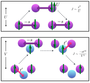
Figure 2: (color online) Spin exchange mechanisms for the Tasaki lattice. The first mechanism is the same that takes place in the Hubbard model and is always antiferromagnetic. The spin flip occurs through an intermediate state of additional energy $U$, as represented in the upper box. In the second mechanism, represented in the lower box, an electron moves to the other sub-lattice, creating a vacancy in the first sub-lattice for another electron. Next, the second electron takes that vacancy. Finally, the first electron occupy the site of the second one. The exchange constant is ferromagnetic if $-s<0$ .

Taking the ground state to be fully polarized along the $z$ direction, the spin Hamiltonian can be mapped into magnon excitations through the Holstein-Primakoff transformation: Holstein and Primakoff (1940)

$$S_{j}^{z} = S-B_{j}^{\dagger}B^{\phantom{\dagger}}_{j},$$ (24)

$$S_{j}^{-} = B_{j}^{\dagger}\left(2S-B_{j}^{\dagger}B^{\phantom{\dagger}}_{j}\right)^{1/2}\approx\sqrt{2S}B_{j}^{\dagger},$$ (25)

$$S_{j}^{+} = \left(2S-B_{j}^{\dagger}B^{\phantom{\dagger}}_{j}\right)^{1/2}B^{\phantom{\dagger}}_{j}\approx\sqrt{2S}B^{\phantom{\dagger}}_{j},$$ (26)

where $S$ is the spin quantum number ($S=1/2$ for electrons), and the magnon operators $B_{j}$ obey a bosonic algebra. We see from Eq. (24) that the number of magnons is directly related to the magnetization.

Within standard linear spin-wave theory, the spin Hamiltonian describes noninteracting magnons and takes the form

$$H_{s}\approx\sum_{k}\omega(k)B_{k}^{\dagger}B^{\phantom{\dagger}}_{k},$$ (27)

with $\omega(k)=2JS(1-\cos k)\approx JSk^{2}$ for $k\ll 1$. The dispersion is gapless because the magnon is the Goldstone mode of the spontaneously broken $SU(2)$ symmetry. From now on, we write simply $\omega(k)\approx\lambda k^{2}$ at low energies. More generally, the effective $\lambda$ away from the strong-coupling limit can be determined within a random phase approximation for the spin-spin correlation function.Mattis (2006) Neglecting interactions between magnons and gapped charge fluctuations, the ferromagnetic Mott-insulating phase at quarter-filling is stable as long as $\lambda>0$.

We are interested in the effects of coupling magnons to gapless charge excitations which arise when we move away from quarter-filling. Since the density of holons is directly related to the density of electrons, adding electrons imply adding holons to the upper Hubbard band. The configurations before and after doping are illustrated in Fig. 3. The doping introduces two Fermi points at $\pm p_{F}$, where $p_{F}$ is related to the average charge density $\rho=\sum_{j,\sigma}\langle n_{j,\sigma}\rangle$ by $p_{F}=\pi(\rho-1/2)$. At energy scales below the charge gap, we can ignore the lower band. Moreover, in the low-doping regime (described by the theory of the commensurate-incommensurate transitionSchulz (1980)) we can neglect holon-holon interactions, which are weak even when $K_{c}\neq 1/2$. The charge Hamiltonian is then simply

$$H_{c} \approx \sum_{p}\epsilon_{c}(p)c_{p}^{\dagger}c_{p},$$ (28)

where $c^{\dagger}_{p}$ creates holons in the upper band and $\epsilon_{c}(p)\approx\gamma p^{2}$ (omitting the constant $\Delta_{c}$ in the energy), with $\gamma\equiv\gamma_{+}$. (Likewise, removing electrons would create holes in the lower band. In this case one would have to replace $\gamma_{+}$ by $\gamma_{-}$ for the low-energy excitations.) We recall that in the strongly interacting regime we expect $\gamma\sim t$, whereas $\lambda\sim J$ with $J$ given in Eq. (23). Therefore, our analysis is valid in the regime $\lambda\ll\gamma$, i.e. when the magnon mass (in the Galilean sense of a quadratic dispersion) is larger than the holon mass.

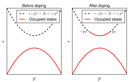
Figure 3: (color online) Holon bands before and after doping the ferromagnetic insulator. At low energies, the dispersion is approximately parabolic. The doping introduces two Fermi points, $-p_{F}$ and $p_{F}$.

We now discuss the interaction between magnons and holons. The form of the interaction can be guessed from symmetry, but before doing so we propose a physical mechanism from which it can be derived. In general, the exchange constant $J$ is a function of the average charge density, $J=J(\rho)$. Following Refs. Matveev, 2004a, b, we consider that in the metallic phase the exchange interaction between neighboring spins is a function of the local density: $H_{s}=\sum_{i}J(\rho_{i})\mathbf{S}_{i}\cdot\mathbf{S}_{i+1}$. In our case, $\rho_{i}$ can fluctuate due to the motion of the dilute electron gas in the even sublattice. Next, we expand $J(\rho_{i})$ around the average density before doping ($\rho_{0}=1/2$): $J(\rho_{i})\approx J(\rho_{0})+\frac{\delta J}{\delta\rho_{i}}\big{|}_{\rho_{i}=\rho_{0}}\delta\rho_{i}$. The term proportional to the derivate of $J$ leads to the spin-charge interaction

$$H_{cs}=\sum_{i}\frac{\delta J(\rho_{i})}{\delta\rho_{i}}\bigg{|}_{\rho_{i}=\rho_{0}}\delta\rho_{i}\mathbf{S}_{i}\cdot\mathbf{S}_{i+1}.$$ (29)

Replacing $\delta\rho_{i}$ by the holon density operator of the upper band, we can write

$$H_{cs}=-\alpha\sum_{i}c^{\dagger}_{i}c^{\phantom{\dagger}}_{i}\mathbf{S}_{i}\cdot\mathbf{S}_{i+1},$$ (30)

where $\alpha\equiv-\left.\frac{\partial J}{\partial\rho}\right|_{\rho_{0}}$ and $c_{i}$ is the Fourier transform of $c_{p}$ in Eq. (28). Using the Holstein-Primakoff transformation again and switching to the momentum representation, we obtain the quartic magnon-holon interaction $H_{I}=\sum_{k,q,p}\zeta(k,p,q)c_{p-q}^{\dagger}c_{p}B_{k+q}^{\dagger}B_{k}$, with

$$\zeta(k,p,q) = -\alpha\left[e^{ik}+e^{-i(k+q)}-e^{-iq}-1\right]$$ (31)

$$\approx \alpha k(k+q).$$

Note that the coupling function is proportional to the momenta of the incoming and the outgoing magnons. Next we discuss how the same form is enforced by symmetry.

Due to spin $SU(2)$ symmetry, the total magnetization $S^{z}_{tot}=\sum_{j}S_{j}^{z}$ is a conserved quantity in our model. Therefore, according to Eq. (24), the number of magnons must also be conserved. This implies that the magnon-holon interaction vertex $\zeta$ must contain one incoming and one outgoing magnon legs (in contrast with the more often encountered coupling between electrons and phonons or photons). By charge conservation, there is also one incoming and one outgoing holon.

Let $p$ and $k$ be the momenta of the incoming holon and magnon, respectively, and $p-q$ and $k+q$ the momenta of the outgoing holon and magnon. In principle, the coupling function $\zeta$ can depend on $p$, $k$ and $q$. Parity symmetry requires that the expansion of $\zeta$ for small $p,k,q$ contains only even powers of momenta. Furthermore, there should be no coupling to magnons with zero momentum (Goldstone bosons) since their presence only amounts to a uniform rotation of the magnetization. Thus, $\zeta\to 0$ if $k\to 0$ or $k+q\to 0$. This rules out a constant term in $\zeta$. The lowest-order term is then a product of two momenta, so we must have $\zeta\propto k(k+q)$. Therefore, the generic form of the magnon-holon interaction in the long-wavelength limit is indeed

$$H_{I}=\alpha\sum_{k,p,q}k(k+q)c^{\dagger}_{p-q}c^{\phantom{\dagger}}_{p}B_{k+q}^{\dagger}B^{\phantom{\dagger}}_{k}.$$ (32)

This result is summarized in Fig. 4.

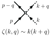
Figure 4: Magnon-holon interaction. Solid (dashed) lines represent holons (magnons). The momentum dependence of the coupling function $\zeta$ is dictated by symmetry.

Our complete Hamiltonian is $H=H_{c}+H_{s}+H_{I}$. To find out how the interaction affects the magnon spectrum, we calculate the magnon self-energy at first and second order in $\alpha$. The corresponding diagrams are illustrated in Fig. 5. In the first-order (“tadpole”) diagram, the holon loop is proportional to the holon density and the interaction vertex contributes with a factor of $k^{2}$. Therefore, the first order diagram only renormalizes the magnon mass, with $\delta\lambda\sim\mathcal{O}(\alpha)$.

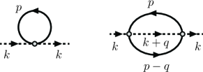
Figure 5: First- and second-order diagrams in the magnon self-energy due to magnon-holon interaction.

The second-order diagram is more interesting. To make the integrals well defined, we introduce a momentum cutoff $D$ around the Fermi points $-p_{F}$ and $p_{F}$ for magnons and holons. We divide the self-energy into two contributions, $\Sigma^{(2)}(k,\omega)=\Sigma_{0}^{(2)}(k,\omega)+\Sigma_{2p_{F}}^{(2)}(k,\omega)$. Both contributions contain logarithmic singularities in their real parts:

$$\Re\Sigma_{0}^{(2)} \sim \alpha^{2}\left(\omega-\lambda k^{2}\right)\log\left(\frac{D}{\omega-\lambda k^{2}}\right),$$

$$\Re\Sigma_{2p_{F}}^{(2)} \sim \alpha^{2}[\omega-\lambda\left(k-2p_{F}\right)^{2}]\log\left[\frac{D}{\omega-\lambda\left(k-2p_{F}\right)^{2}}\right]$$ (33)

$$+(p_{F}\to-p_{F}).$$

The first contribution arises from low-momentum scattering and is typical of the orthogonality catastrophe, which has already been studied in the case of bosons. Zvonarev et al. (2007); Kamenev and Glazman (2009) The second contribution corresponds to a momentum transfer of $2p_{F}$; it diverges on-shell only if $|k\pm 2p_{F}|\approx|k|$, where $k$ is the magnon momentum. These singularities tell us some important mechanism is taking place when magnons and holons scatter around the Fermi points.

IV Effective field theory for magnon-holon interaction

In this section, we derive an effective field theory for the scattering between holons and magnons with momentum close to the Fermi points $\pm p_{F}$. Our goal is to enlighten the mechanism behind the infrared singularities encountered in Sec. III and to set the stage for going beyond perturbation theory using the numerical renormalization group in Sec. V.

IV.1 Chirality Kondo effect

We start by rewriting the free Hamiltonians of Eq. (27) and (28) in the continuum limit in terms of holon and magnon fields:

$$H_{c}=\gamma\int dx\leavevmode\nobreak\ \partial_{x}\psi^{\dagger}(x)\partial_{x}\psi(x),$$ (34)

$$H_{s}=\lambda\int dx\leavevmode\nobreak\ \partial_{x}B^{\dagger}(x)\partial_{x}B(x).$$ (35)

where $\psi(x)=\frac{1}{\sqrt{L}}\sum_{p}c_{p}e^{ipx}$ and $B(x)=\frac{1}{\sqrt{L}}\sum_{k}B_{k}e^{ikx}$, with $L$ the system size.

We now restrict to low energies compared with the holon Fermi energy $\lambda p_{F}^{2}$. In this regime holons can only be scattered in the vicinity of the Fermi points. We expand the holon fields in terms of left movers and right movers,

$$\psi(x)\approx e^{-ip_{F}x}\psi_{L}(x)+e^{ip_{F}x}\psi_{R}(x).$$ (36)

We also focus on magnon states with momentum near $\pm p_{F}$, and expand

$$B(x)\approx e^{-ip_{F}x}B_{L}(x)+e^{ip_{F}x}B_{R}(x).$$ (37)

We define two-component spinor fields which combine right and left movers

$$\Psi(x)=\left(\begin{array}[]{c}\psi_{R}(x)\\ \psi_{L}(x)\end{array}\right),\quad\Omega(x)=\left(\begin{array}[]{c}B_{R}(x)\\ B_{L}(x)\end{array}\right).$$ (38)

Linearizing both holon and magnon dispersion for $k,p\approx\pm p_{F}$ (and measuring the holon dispersion from the Fermi energy), we can write

$$H_{c} \approx \int dx\leavevmode\nobreak\ \Psi^{\dagger}(x)\left(-iv\tau^{z}\partial_{x}\right)\Psi(x),$$ (39)

$$H_{s} \approx \int dx\leavevmode\nobreak\ \Omega^{\dagger}(x)\left[\omega(p_{F})-iu\tau^{z}\partial_{x}\right]\Omega(x),$$ (40)

where $v=2\gamma p_{F}$ and $u=2\lambda p_{F}$ are the holon and magnon velocities, respectively, and $\tau^{z}$ is the $z$ Pauli matrix in the internal chirality space. As discussed in Sec. III, we expect $\lambda\ll\gamma$ in the limit $J\ll s,t$. Thus, we are in a “slow magnon” regime $u\ll v$. The spinor representation suggests regarding the chirality indices as pseudospins, $R=\leavevmode\nobreak\ \uparrow$ and $L=\leavevmode\nobreak\ \downarrow$ (not to be confused with the original electron spin $\sigma$). We will see soon that this picture is useful to interpret the interaction, but it is important to keep in mind that the physical meaning of $R$ ($L$) is that the particle carries momentum close to $p_{F}$ ($-p_{F}$).

Now we must propose the form of the magnon-holon interaction. As before, we appeal to symmetries. As we discussed in Sec. III, conservation of magnetization implies that a local interacting term must have the general form $\psi_{r_{1}}^{\dagger}(x)\psi^{\phantom{\dagger}}_{r_{2}}(x)B^{\dagger}_{r_{3}}(x)B^{\phantom{\dagger}}_{r_{4}}(x)$ in order to conserve the number of magnons. In this notation, $r$ represents a pseudospin index ($R$ or $L$). Momentum conservation impose constraints on the $r$’s: only combinations such that $r_{1}-r_{2}+r_{3}-r_{4}=0$ are allowed. These are: $LLLL$ and $RRRR$; $LLRR$ and $RRLL$; and $LRRL$ and $RLLR$. We split them into pairs related by a parity transformation (where $L\leftrightarrow R$). To ensure parity symmetry, coupling constants for each element of a pair must be the same. The corresponding scattering processes are illustrated in Fig. 6.

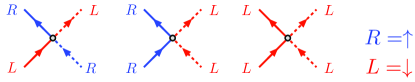
Figure 6: (color online) Different kinds of fermion-magnon scattering around the Fermi levels. The indices $L$ and $R$ indicate whether the particle momentum is closest to $-p_{F}$ or $p_{F}$. By defining a chirality pseudospin such that $R=\leavevmode\nobreak\ \uparrow$ and $L=\leavevmode\nobreak\ \downarrow$, the scattering can be identified with pseudospin exchange interaction (as represented by the diagrams on the bottom). The solid line represent holons and the dashed line represent magnons. There are in fact six diagrams, but the remaining ones can be obtained from the ones presented through a parity transformation.

With these restrictions, it is not difficult to show that, in the spinor representation, the interacting part of the Hamiltonian assumes the form

$$H_{I} = V\int dx\leavevmode\nobreak\ \Psi^{\dagger}\Psi\Omega^{\dagger}\Omega+\frac{J_{\parallel}}{4}\int dx\leavevmode\nobreak\ \Psi^{\dagger}\tau^{z}\Psi\Omega^{\dagger}\tau^{z}\Omega$$ (41)

$$+\frac{J_{\perp}}{8}\int dx\leavevmode\nobreak\ (\Psi^{\dagger}\tau^{+}\Psi\,\Omega^{\dagger}\tau^{-}\Omega+{\text{H.\ c.}}),$$

where $V,J_{\parallel},J_{\perp}$ are three independent coupling constants. Since this interaction term must arise from linearizing Eq. (52), we expect the coupling constants to be of the order of $\alpha p_{F}^{2}$.

In terms of pseudospins, the first term in Eq. (41) describes the potential scattering between holons and magnons, while the remaining terms describe an anisotropic exchange interaction between holon and magnon pseudospins. Recognizing $\mathbf{S}_{F}(x)\equiv\Psi^{\dagger}(x)\frac{\boldsymbol{\tau}}{2}\Psi(x)$ and $\mathbf{S}_{M}(x)\equiv\Omega^{\dagger}(x)\frac{\boldsymbol{\tau}}{2}\Omega(x)$ as pseudospin vector densities, we further rewrite $H_{I}$ as

$$H_{I} = V\int dx\leavevmode\nobreak\ \Psi^{\dagger}\Psi\Omega^{\dagger}\Omega+J_{\parallel}\int dx\leavevmode\nobreak\ S_{F}^{z}(x)S_{M}^{z}(x)$$ (42)

$$+\frac{J_{\perp}}{2}\int dx\leavevmode\nobreak\ \left[S_{F}^{+}(x)S_{M}^{-}(x)+{\text{H.\ c.}}\right],$$

where the label $F$ is for (fermionic) holons and the label $M$ is for magnons.

The Hamiltonian in Eq. (42) can be viewed as a Kondo interactionHewson (1997) between a finite density of fermions (represented by the holons) and a number of mobile impurities (represented by the magnons). The connection with the Kondo model is made more clear in the limit of vanishing magnon density (which is the interesting regime to investigate the stability of the ferromagnetic state against infinitesimal perturbations). Since magnetization is conserved, we may restrict our problem to the subspace with a single magnon. In this case we can rewrite the Hamiltonian using first quantization for magnon operators:

$$H_{s} = \omega(p_{F})+2uS_{M}^{z}\hat{P},$$ (43)

$$H_{I} = V\Psi^{\dagger}(\hat{X})\Psi(\hat{X})+J_{\parallel}S_{F}^{z}(\hat{X})S_{M}^{z}$$ (44)

$$+\frac{J_{\perp}}{2}\left[S_{F}^{+}(\hat{X})S_{M}^{-}+{\text{H.\ c.}}\right],$$

where $\hat{X}$ and $\hat{P}$ are the position and momentum operators of the magnon, respectively, obeying $[\hat{X},\hat{P}]=i$. Note that the Hamiltonian is translationally invariant, but the interaction is local at the position of the magnon. This kind of dynamics has been encountered in the coupling of a mobile impurity with a Luttinger liquid.Lamacraft (2009)

Next, we apply a Galilean transformation to the magnon reference frame.Lee et al. (1953); Castro Neto and Fisher (1996) The transformation is

$$U\equiv e^{-i\hat{X}\int dx\,\Psi^{\dagger}(-i\partial_{x})\Psi},$$ (45)

and is such that

$$\tilde{\Psi}(x) = U^{\dagger}\Psi(x)U=\Psi(x-\hat{X}),$$ (46)

$$\tilde{P} = U^{\dagger}\hat{P}U=\hat{P}-\int dx\,\Psi^{\dagger}(-i\partial_{x})\Psi.$$ (47)

As a result, the transformed interaction $\tilde{H}_{I}=U^{\dagger}H_{I}U$ becomes

$$\tilde{H}_{I} = V\Psi^{\dagger}(0)\Psi(0)+J_{\parallel}S^{z}_{F}(0)S^{z}_{M}$$ (48)

$$+\frac{J_{\perp}}{2}\left[S^{+}_{F}(0)S^{-}_{M}+{\text{H.\ c.}}\right].$$

The magnon-holon interaction is now restricted to $x=0$, since we are in a frame whose origin moves along with the magnon. For consistency, we must also transform the kinetic energy terms $H_{c}$ and $H_{s}$. The free holon Hamiltonian remains unchanged, i. e., $\tilde{H}_{c}=H_{c}$. However, the magnon term in Eq. (43) gets modified:

$$\tilde{H}_{s} = U^{\dagger}H_{s}U$$ (49)

$$= \omega(p_{F})+2uS_{M}^{z}\hat{P}+2iuS_{M}^{z}\int dx\,\Psi^{\dagger}\partial_{x}\Psi.$$

At this point we have eliminated the magnon position $\hat{X}$ from the transformed Hamiltonian $\tilde{H}=\tilde{H}_{c}+\tilde{H}_{s}+\tilde{H}_{I}$. Therefore, $[\tilde{H},\hat{P}]=0$, implying that $\tilde{H}$ and $\hat{P}$ can be simultaneously diagonalized. This is a consequence of translational invariance of the original Hamiltonian.Lee et al. (1953); Castro Neto and Fisher (1996) We shall focus on the subspace with eigenvalue $P=0$, which corresponds to a magnon with energy exactly equal to $\omega(p_{F})$. In this case the first term in Eq. (49) vanishes. Deviations from the $P=0$ condition amount to an extra term proportional to $S_{M}^{z}$, which is equivalent to an effective magnetic field acting on the magnon pseudospin. While we have got rid of $\hat{X}$, the price we paid is the introduction of the second term in Eq. (49). This term couples the magnon pseudospin to the total momentum operator for holons.

We can now add $\tilde{H}_{s}$ for $P=0$ to the free holon Hamiltonian $\tilde{H}_{c}$:

$$\tilde{H}_{c}+\tilde{H}_{s} = \omega(p_{F})+\int dx\,\psi^{\dagger}_{R}(v-2uS_{M}^{z})(-i\partial_{x})\psi^{\phantom{\dagger}}_{R}$$ (50)

$$+\int dx\,\psi^{\dagger}_{L}(v+2uS_{M}^{z})(i\partial_{x})\psi^{\phantom{\dagger}}_{L}.$$

We further rewrite the right-hand side of Eq. (50) by taking $\psi_{L}(x)\to\psi_{L}(-x)$ (this is equivalent to relabeling holon states with momentum $p$ as $-p$ for the left branch):

$$\tilde{H}_{c}+\tilde{H}_{s}=\omega(p_{F})+\int dx\,\Psi^{\dagger}(v-2uS^{z}_{M}\tau^{z})(-i\partial_{x})\Psi.$$ (51)

We emphasize that $\tau^{z}$ in Eq. (51) acts in the holon pseudospin space. Recall that $v$ is the holon velocity around the Fermi points $\pm p_{F}$. Eq. (51) shows that the holon velocity in the transformed Hamiltonian is now given by $v\pm u$ depending on whether the holon and magnon have the same or opposite pseudospins, i. e. move in the same or opposite directions.

Finally, dropping the constant $\omega(p_{F})$ and adding the transformed interaction of Eq. (48), we arrive at our effective Kondo-type Hamiltonian for the scattering of a single magnon with momentum close to $\pm p_{F}$ by low-energy holons:

$$\tilde{H} = \sum_{k=-\infty}^{+\infty}\Psi_{k}^{\dagger}\left(v-2uS^{z}_{M}\tau^{z}\right)k\leavevmode\nobreak\ \Psi_{k}$$ (52)

$$+\frac{J_{\perp}}{2}[S^{+}_{F}(0)S^{-}_{M}+{\text{H.\ c.}}]$$

$$+J_{\parallel}S^{z}_{F}(0)S^{z}_{M}+V\Psi^{\dagger}(0)\Psi(0).$$

IV.2 Perturbative renormalization group analysis

If the magnon had zero velocity, i. e., $u=0$, the model of Eq. (52) would correspond precisely to the Kondo model, which describes a Fermi sea of electrons coupled to a spin-$1/2$ impurity at the origin through an anisotropic exchange interaction. Hewson (1997) Here the model also includes the potential scattering $V$, which is generally present in the absence of particle-hole symmetry. It is well known that perturbation theory in the Kondo interaction gives rise to infrared divergences like the ones we encountered in Eq. (III). The Kondo model has been investigated non-perturbatively using the numerical renormalization group (NRG) Krishna-murthy et al. (1980a); Bulla et al. (2008) and solved exactly through Bethe ansatz.Andrei et al. (1983) From the renormalization group (RG) point of view, the logarithmic singularities that arise in perturbation theory can be recast in the renormalization of effective coupling constants at the appropriate energy scale. For $u=0$, the exchange coupling constants flow to strong coupling if $J_{\perp}>-J_{\parallel}$. The low-energy fixed point of the model can be understood in terms of the formation of a singlet between the localized impurity and one electron from the conduction band, which decouples from the remaining electrons. In other words, the fermion spin screens the impurity spin.

In our case, the renormalization of the effective exchange interactions decides the fate of the magnon in the low-energy limit. We first approach the problem by applying a perturbative RG approach to interaction (41) with $u>0$. The procedure is similar to Anderson’s poor man’s scaling,Anderson (1970) generalized to include a momentum cutoff in the magnon sub-band and to respect total momentum conservation in the virtual magnon-holon scattering process. We obtain the set of RG equations:

$$\frac{dJ_{\perp}}{d\ell} = \frac{vJ_{\perp}(J_{\parallel}-V)}{2\pi(v^{2}-u^{2})},$$ (53)

$$\frac{d(J_{\parallel}-V)}{d\ell} = \frac{J_{\perp}^{2}}{2\pi(v+u)},$$ (54)

$$\frac{d(J_{\parallel}+V)}{d\ell} = \frac{J_{\perp}^{2}}{2\pi(v-u)},$$ (55)

$$\frac{du}{d\ell} = -\frac{uJ_{\perp}^{2}}{8\pi(v^{2}-u^{2})},$$ (56)

where $d\ell=d\Lambda/\Lambda$ denotes the infinitesimal reduction of the ultraviolet cutoff in the RG step.

To analyze the RG flow, we first note that to second order in perturbation theory the renormalization of $J_{\parallel}+V$ is controlled by $J_{\perp}$ and does not feed back into the beta functions for $J_{\perp}$ and $J_{\parallel}-V$. We can then focus on Eqs. (53) and (54). In the slow magnon regime $u<v$, these coupled equations define a Kosterlitz-Thouless type flow diagram in the $(J_{\perp},J_{\parallel}-V)$ plane, with a flow to strong coupling for $J_{\perp}>-(J_{\parallel}-V)$. Furthermore, Eq. (56) implies that the magnon velocity decreases with the RG flow. Here we should remark that we can follow the flow to arbitrarily low energies only in the case $P=0$, i. e. when the magnon momentum exactly matches the holon Fermi momentum $p_{F}$. As discussed in Sec. IV.1, deviations from this condition are equivalent to an effective magnetic field coupled to the magnon pseudospin, which cuts off the RG flow at the scale set by $P$.

The enhancement of the effective couplings suggests that in the low-energy limit the magnon is strongly backscattered between states with momentum $\pm p_{F}$, and its group velocity may eventually vanish as suggested by Eq. (56). By analogy with the original Kondo effect, we expect that at the low-energy fixed point the magnon will form a “chirality singlet” with one holon, as represented by the state $|\Phi\rangle=\frac{1}{\sqrt{2}}\int dx[B^{\dagger}_{R}(x)\psi^{\dagger}_{L}(x)-B^{\dagger}_{L}(x)\psi^{\dagger}_{R}(x)]|0\rangle$. This singlet involves a pair of (distinguishable) particles which are delocalized in space and move with opposite momenta — somewhat akin to a Cooper pair in BCS theory. Note that the particle-hole symmetry of our model is broken both by $V\neq 0$ and $u\neq 0$; thus, the putative low-energy fixed point should contain a marginal potential scattering operator that accounts for a non-universal phase shift in the remaining holon states. In Sec. V we shall investigate the nature of the low-energy fixed point using the NRG method.

V Numerical renormalization group

The numerical diagonalization of the Hamiltonian (52) follows the standard NRG method. The procedure having been thoroughly detailed, Krishna-murthy et al. (1980a); Bulla et al. (2008) only cursory description is necessary, meant to prepare the discussion of the flow in renormalization-group space that constitutes the central object of this section.

V.1 Procedure

To diagonalize the Hamiltonian (52), we will rely on the numerical renormalization-group procedure, an approximate iterative method that depends on strictly controllable approximations to yield a set of eigenvalues and eigenvectors from which essentially exact physical properties. More important from our perspective, the iterative diagonalization can be regarded as a sequence of renormalization-group transformations and therefore accurately describes the flow of the Hamiltonian in renormalization-group space.

To define the renormalization-group transformation, we need a scaled truncated version of the Hamiltonian. Our initial goal is to project Eq. (52) on a finite basis. Relative to the basis of the holon and magnon states, the new basis will of course be incomplete. Special care will be taken to preserve the magnon states and their interaction with the holons. Only the first term on the right-hand side of Eq. (52) will be affected by the projection, which comprises three steps.

V.1.1 Logarithmic discretization of the conduction band

The first step is controlled by an arbitrary dimensionless parameter $\Lambda>1$. Given $\Lambda$, we split the conduction band into two segments, one above and the other below the Fermi level, and divide each segment into an infinite logarithmic sequence of intervals

$$\mathcal{I}_{m\pm}=\pm D\big{(}\Lambda^{-m-1},\Lambda^{-m}\big{)}\qquad(m=0,1,\ldots),$$ (57)

where the positive segment runs from $\epsilon_{k}=\epsilon_{F}\equiv 0$ to $\epsilon_{k}=D$, and the negative one from $\epsilon_{k}=-D$ to $\epsilon_{k}=0$.

For each interval $\mathcal{I}_{m\pm}$, we define the normalized Fermi operator

$$a_{m\pm}=\dfrac{\Lambda^{m/2}}{\sqrt{1-\Lambda^{-1}}}\sum_{k\in\mathcal{I}_{m\pm}}\Psi_{k}\qquad(m=0,1,\ldots).$$ (58)

It follows that the operator $\Psi(0)$ is a linear combination of the $a_{m\pm}$:

$$\Psi(0)=\sqrt{1-\Lambda^{-1}}\sum_{m=0}^{\infty}\Lambda^{-m/2}\left(a_{m+}+a_{m-}\right)\equiv\sqrt{2}f_{0}^{\phantom{\dagger}},$$ (59)

where we have defined the normalized Fermi operator $f_{0}^{\phantom{\dagger}}$, so that Eq. (52) can be written in the exact form

$$\tilde{H}= \sum_{k}\Psi_{k}^{\dagger}(v-2uS^{z}_{M}\tau^{z})\Psi_{k}+J_{\perp}\left(f_{0\uparrow}^{\dagger}f_{0\downarrow}^{\phantom{\dagger}}S^{-}_{M}+{\text{H.\ c.}}\right)$$

$$+2J_{\parallel}\left(f_{0\uparrow}^{\dagger}f_{0\uparrow}^{\phantom{\dagger}}-f_{0\downarrow}^{\dagger}f_{0\downarrow}^{\phantom{\dagger}}\right)S^{z}_{M}$$

$$+2V\left(f_{0\uparrow}^{\dagger}f_{0\uparrow}^{\phantom{\dagger}}+f_{0\downarrow}^{\dagger}f_{0\downarrow}^{\phantom{\dagger}}\right).$$ (60)

Here $\uparrow=R$ and $\downarrow=L$ refer to the chirality pseudospins defined in Sec. IV. From now on we shall call these simply “holon spins”, whereas $\mathbf{S}_{M}$ is the “magnon spin”.

Next, we project the first term on the right-hand side of Eq. (60) on the basis of the $a_{m\pm}^{\phantom{\dagger}}$, which yields the approximate equality

$$\tilde{H} = \sum_{m}\mathcal{E}_{m}\left[v(a_{m\uparrow}^{\dagger}a_{m\uparrow}^{\phantom{\dagger}}+a_{m\downarrow}^{\dagger}a_{m\downarrow}^{\phantom{\dagger}})\right.$$ (61)

$$\left.-2u(a_{m\uparrow}^{\dagger}a_{m\uparrow}^{\phantom{\dagger}}-a_{m\downarrow}^{\dagger}a_{m\downarrow}^{\phantom{\dagger}})S^{z}_{M}\right]$$

$$+J_{\perp}\left(f_{0\uparrow}^{\dagger}f_{0\downarrow}^{\phantom{\dagger}}S^{-}_{M}+{\text{H.\ c.}}\right)$$

$$+2J_{\parallel}\left(f_{0\uparrow}^{\dagger}f_{0\uparrow}^{\phantom{\dagger}}-f_{0\downarrow}^{\dagger}f_{0\downarrow}^{\phantom{\dagger}}\right)S^{z}_{M}$$

$$+2V\left(f_{0\uparrow}^{\dagger}f_{0\uparrow}^{\phantom{\dagger}}+f_{0\downarrow}^{\dagger}f_{0\downarrow}^{\phantom{\dagger}}\right),$$

where

$$\mathcal{E}_{m}=\dfrac{1-\Lambda^{-1}}{\log\Lambda}\Lambda^{-m}$$ (62)

is the average momentum in the interval $\mathcal{I}_{m}$.Campo and Oliveira (2005)

The projection on the incomplete basis introduces deviations in computed physical properties of $\mathcal{O}[\exp(-\dfrac{\pi^{2}}{\log\Lambda})]$,Krishna-murthy et al. (1980a) which are insignificant for $\Lambda\lesssim 3$.

V.1.2 Lanczos transformation

Numerical treatment of the Hamiltonian (61) calls for truncation of the infinite basis. To preserve the interaction terms on the right-hand side, before truncation we define a new infinite basis $\{f_{n}^{\phantom{\dagger}}\}$ ($n=0,1,\ldots$), where the Fermi operators $f_{n}^{\phantom{\dagger}}$ form an orthonormal sequence of linear combinations of the $a_{m\pm}^{\phantom{\dagger}}$,

$$f_{n}^{\phantom{\dagger}}=\sum_{m=0}^{\infty}\alpha_{nm}\Big{[}a_{m+}+(-1)^{n}a_{m-}\Big{]}.$$ (63)

In the new basis, $f_{0}^{\phantom{\dagger}}$ is the operator defined by Eq. (59), so that

$$\alpha_{0m}=\sqrt{\dfrac{1-\Lambda^{-1}}{2}}\Lambda^{-m/2},$$ (64)

and the remaining Fermi operators are tailored to the requirement that

$$\sum_{m=0}^{\infty}\mathcal{E}_{m}(a_{m+}^{\dagger}a_{m+}^{\phantom{\dagger}}-a_{m-}^{\dagger}a_{m-}^{\phantom{\dagger}})=\sum_{n=0}^{\infty}t_{n}(f_{n}^{\dagger}f_{n+1}^{\phantom{\dagger}}+{\text{H.\ c.}}).$$ (65)

Wilson has shown that Eq. (65) is satisfied withWilson (1975)

$$t_{n}=\dfrac{\mathcal{E}_{0}(1-\Lambda^{-n-1})\Lambda^{-n/2}}{\sqrt{(1-\Lambda^{-2n-1})(1-\Lambda^{-2n-3})}}\qquad(n=0,1,\ldots)$$ (66)

and determined the coefficients $\alpha_{nm}$. In particular, for $n=1$,

$$\alpha_{1m}=\sqrt{\dfrac{1-\Lambda^{-3}}{2}}\Lambda^{-3m/2}.$$ (67)

We now substitute the right-hand side of Eq. (65) for the kinetic terms on the right-hand side of Eq. (61), to obtain the Lanczos transformed Hamiltonian

$$\tilde{H}= \sum_{n=0}^{\infty}t_{n}\left[v(f_{n\uparrow}^{\dagger}f_{n+1\uparrow}^{\phantom{\dagger}}+f_{n\downarrow}^{\dagger}f_{n+1\downarrow}^{\phantom{\dagger}})\right.$$

$$\left.-2u(f_{n\uparrow}^{\dagger}f_{n+1\uparrow}^{\phantom{\dagger}}-f_{n\downarrow}^{\dagger}f_{n+1\downarrow}^{\phantom{\dagger}})S^{z}_{M}+{\text{H.\ c.}}\right]$$

$$+J_{\perp}\left(f_{0\uparrow}^{\dagger}f_{0\downarrow}^{\phantom{\dagger}}S^{-}_{M}+{\text{H.\ c.}}\right)$$

$$+2J_{\parallel}\left(f_{0\uparrow}^{\dagger}f_{0\uparrow}^{\phantom{\dagger}}-f_{0\downarrow}^{\dagger}f_{0\downarrow}^{\phantom{\dagger}}\right)S^{z}_{M}$$

$$+2V\left(f_{0\uparrow}^{\dagger}f_{0\uparrow}^{\phantom{\dagger}}+f_{0\downarrow}^{\dagger}f_{0\downarrow}^{\phantom{\dagger}}\right),$$ (68)

which leaves us in position to truncate the infinite basis.

V.1.3 Truncation and scaling

Inspection of Eq. (66) shows that the fraction on the right-hand side rapidly approaches unity as $n$ grows, so that to an excellent approximation,

$$t_{n}=\mathcal{E}_{0}\Lambda^{-n/2}\qquad(n\ \mathrm{such\ that}\ \Lambda^{-n}\ll 1).$$ (69)

If we are interested in physical properties at the energy scale $E$, it is safe to truncate the infinite series on the right-hand side of Eq. (68) at $n=N$, where $N$ is the smallest integer satisfying $t_{N}<\epsilon_{IR}E$ for a specified dimensionless infrared cutoff $\epsilon_{IR}^{\phantom{\dagger}}\ll 1$. Given an energy $E$ and an infrared cutoff $\epsilon_{IR}^{\phantom{\dagger}}$, we define the truncated, scaled Hamiltonian

$$H_{N}\equiv\dfrac{1}{\mathcal{D}_{N-1}}\Bigg{\{} \sum_{n=0}^{N-1}t_{n}\left[v(f_{n\uparrow}^{\dagger}f_{n+1\uparrow}^{\phantom{\dagger}}+f_{n\downarrow}^{\dagger}f_{n+1\downarrow}^{\phantom{\dagger}})\right.$$

$$\left.-2u(f_{n\uparrow}^{\dagger}f_{n+1\uparrow}^{\phantom{\dagger}}-f_{n\downarrow}^{\dagger}f_{n+1\downarrow}^{\phantom{\dagger}})S^{z}_{M}+{\text{H.\ c.}}\right]$$

$$+J_{\perp}\left(f_{0\uparrow}^{\dagger}f_{0\downarrow}^{\phantom{\dagger}}S^{-}_{M}+{\text{H.\ c.}}\right)$$

$$+2J_{\parallel}\left(f_{0\uparrow}^{\dagger}f_{0\uparrow}^{\phantom{\dagger}}-f_{0\downarrow}^{\dagger}f_{0\downarrow}^{\phantom{\dagger}}\right)S^{z}_{M}$$

$$+2V\left(f_{0\uparrow}^{\dagger}f_{0\uparrow}^{\phantom{\dagger}}+f_{0\downarrow}^{\dagger}f_{0\downarrow}^{\phantom{\dagger}}\right)\Bigg{\}},$$ (70)

where $\mathcal{D}_{n}$ denotes the right-hand side of Eq. (69), i. e., $\mathcal{D}_{n}\equiv\mathcal{E}_{0}\Lambda^{-n/2}$.

V.1.4 Iterative diagonalization

The truncated form (V.1.3) is convenient for iterative diagonalization.Krishna-murthy et al. (1980a) With $N=1$, only the magnon spin and the operators $f_{0}^{\phantom{\dagger}}$ and $f_{1}^{\phantom{\dagger}}$ contributing to the right-hand side, the Hamiltonian $H_{N=1}$ is equivalent to a $32\times 32$ matrix that is easily diagonalized, numerically. The next Hamiltonian in the iterative procedure, $H_{N=2}$ is then projected on the basis $\mid r\rangle_{1}$, $f_{N+2\uparrow}^{\dagger}\mid r\rangle_{1}$, $f_{N+2\downarrow}^{\dagger}\mid r\rangle_{1}$, $f_{N+2\uparrow}^{\dagger}f_{N+2\downarrow}^{\dagger}\mid r\rangle_{1}$ ($r=1,2,\ldots,32$), where $\mid r\rangle_{1}$ is one of the eigenstates resulting from the diagonalization of $H_{N=1}$, and the resulting $128\times 128$ matrix is numerically diagonalized. This completes the first iterative cycle ($N=2$).

More generally, given the eigenstates $\mid r\rangle_{N}$ of $H_{N}$, the Hamiltonian $H_{N+1}$ is projected on the basis resulting from the operators $\mathds{1}$, $f_{N+1\uparrow}^{\dagger}$, $f_{N+1\downarrow}^{\dagger}$, and $f_{N+1\uparrow}^{\dagger}f_{N+1\downarrow}^{\dagger}$ applied to the $\mid r\rangle_{N}$ and diagonalized. The number of eigenstates of $H_{N}$ in the first few iterations is $N_{r}=2^{1+2N}$. To keep the rapidly growing $N_{r}$ under control, only the eigenstates of $H_{N}$ corresponding to eigenvalues below a fixed ultraviolet cutoff $E_{uv}$ are computed at each iteration, so that the computational cost grows linearly, instead of exponentially, with the number of iterations. The ultraviolet cutoff $E_{uv}$, the discretization parameter $\Lambda$ and the infrared cutoff $\epsilon_{IR}^{\phantom{\dagger}}$ control the computational cost and the accuracy of the physical properties calculated from the eigenstates and eigenvalues of $H_{N}$.

V.1.5 Renormalization-group transformation

The factor $1/\mathcal{D}_{N-1}$ on the right-hand side of Eq. (V.1.3) expresses the Hamiltonian $H_{N}$ in units of its smallest matrix element, $t_{N-1}\approx\mathcal{D}_{N-1}$ and defines a renormalization-group transformation $\mathcal{T}$, which turns a scaled truncated Hamiltonian into another scaled Hamiltonian, one that is truncated at a finer scale. More specifically, from Eq. (V.1.3) we have that

$$H_{N+2}= \Lambda H_{N}+\sum_{n=N}^{N+1}\dfrac{t_{n}}{\mathcal{D}_{N+1}}\Big{[}v(f_{n\uparrow}^{\dagger}f_{n+1\uparrow}^{\phantom{\dagger}}+f_{n\downarrow}^{\dagger}f_{n+1\downarrow}^{\phantom{\dagger}})$$

$$-2u(f_{n\uparrow}^{\dagger}f_{n+1\uparrow}^{\phantom{\dagger}}-f_{n\downarrow}^{\dagger}f_{n+1\downarrow}^{\phantom{\dagger}})S^{z}_{M}+{\text{H.\ c.}}\Big{]},$$ (71)

which defines the transformation $\mathcal{T}[H_{N}]=H_{N+2}$.

At first sight, it may seem more natural to step $N\to N+1$. Nonetheless, the $H_{N}\to H_{N+1}$ transformation is unwieldy, because successive applications almost invariably generate two-point limit cycles.Krishna-murthy et al. (1980a) The $H_{N}\to H_{N+2}$ transformation, by contrast, has simple fixed points.

V.2 Fixed points

As first shown by Wilson,Wilson (1975) the spin-flip term on the right-hand side of Eq. (52) is a marginally relevant operator. To identify the fixed points of $\mathcal{T}[H_{N}]$ we will therefore consider two forms of the Hamiltonian that remain invariant under scaling of $J_{\perp}$. For weak coupling between the magnon and the holons, for small $N$ the scaled truncated Hamiltonian $H_{N}$ in Eq. (V.1.3) tends to be close to one of them. As $N$ grows, our numerical analysis shows that $H_{N}$ flows towards the second fixed point. We will therefore refer to the former (latter) as the weak-coupling (strong-coupling) fixed points.

V.2.1 Weak-coupling fixed points ($J_{\perp}=0$)

Without the spin-flip term, the Hamiltonian (V.1.3) reads

$$\mathcal{D}_{N-1}H_{N}^{0}= \sum_{n=0}^{N-1}t_{n}\left[v(f_{n\uparrow}^{\dagger}f_{n+1\uparrow}^{\phantom{\dagger}}+f_{n\downarrow}^{\dagger}f_{n+1\downarrow}^{\phantom{\dagger}})\right.$$

$$\left.-2u(f_{n\uparrow}^{\dagger}f_{n+1\uparrow}^{\phantom{\dagger}}-f_{n\downarrow}^{\dagger}f_{n+1\downarrow}^{\phantom{\dagger}})S^{z}_{M}+{\text{H.\ c.}}\right]$$

$$+2J_{\parallel}\left(f_{0\uparrow}^{\dagger}f_{0\uparrow}^{\phantom{\dagger}}-f_{0\downarrow}^{\dagger}f_{0\downarrow}^{\phantom{\dagger}}\right)S^{z}_{M}$$

$$+2V\left(f_{0\uparrow}^{\dagger}f_{0\uparrow}^{\phantom{\dagger}}+f_{0\downarrow}^{\dagger}f_{0\downarrow}^{\phantom{\dagger}}\right),$$ (72)

a form that commutes with $S^{z}_{M}$.

The spectrum of $H_{N}^{0}$ can therefore be classified by the $z$ component $s^{z}_{M}$ of the magnon spin. It can be divided, in other words, into an $s^{z}_{M}=1/2$ sector and another with $s^{z}_{M}=-1/2$.

For each magnon-spin component, the Hamiltonian in Eq. (72) splits into an $\uparrow$ and a $\downarrow$ terms, labeled by the holon spin. For $s^{z}_{M}=+1/2$, we have that

$$H_{N}^{0}=H_{N,\uparrow}^{0+}+H_{N,\downarrow}^{0+},$$ (73)

where

$$\mathcal{D}_{N-1}H_{N,\uparrow}^{0+}= (v-u)\sum_{n=0}^{N-1}t_{n}(f_{n\uparrow}^{\dagger}f_{n+1\uparrow}^{\phantom{\dagger}}+{\text{H.\ c.}})$$

$$+(2V+J_{\parallel})f_{0\uparrow}^{\dagger}f_{0\uparrow}^{\phantom{\dagger}}$$ (74)

and

$$\mathcal{D}_{N-1}H_{N,\downarrow}^{0+}= (v+u)\sum_{n=0}^{N-1}t_{n}(f_{n\downarrow}^{\dagger}f_{n+1\downarrow}^{\phantom{\dagger}}+{\text{H.\ c.}})$$

$$+(2V-J_{\parallel})f_{0\downarrow}^{\dagger}f_{0\downarrow}^{\phantom{\dagger}}.$$ (75)

With $s^{z}_{M}=-1/2$, the Hamiltonian (73) likewise splits in two terms:

$$H_{N}^{0}=H_{N,\uparrow}^{0-}+H_{N,\downarrow}^{0-},$$ (76)

where

$$\mathcal{D}_{N-1}H_{N,\uparrow}^{0-}= (v+u)\sum_{n=0}^{N-1}t_{n}(f_{n\uparrow}^{\dagger}f_{n+1\uparrow}^{\phantom{\dagger}}+{\text{H.\ c.}})$$

$$+(2V-J_{\parallel})f_{0\uparrow}^{\dagger}f_{0\uparrow}^{\phantom{\dagger}},$$ (77)

and

$$\mathcal{D}_{N-1}H_{N,\downarrow}^{0-}= (v-u)\sum_{n=0}^{N-1}t_{n}(f_{n\downarrow}^{\dagger}f_{n+1\downarrow}^{\phantom{\dagger}}+{\text{H.\ c.}})$$

$$+(2V+J_{\parallel})f_{0\downarrow}^{\dagger}f_{0\downarrow}^{\phantom{\dagger}}.$$ (78)

Comparison of the right-hand sides of Eqs. (V.2.1) and (V.2.1) shows that $H_{N,\uparrow}^{0+}$ and $H_{N,\downarrow}^{0-}$ transform into each other under the inversion $f_{n\uparrow}^{\phantom{\dagger}}\leftrightarrow f_{n\downarrow}^{\phantom{\dagger}}$ and therefore have the same spectrum. Likewise, $H_{N,\uparrow}^{0-}$ and $H_{N,\downarrow}^{0+}$ transform into each other under the same inversion and have identical spectra.

In fact, the four Hamiltonians, $H_{N,\uparrow}^{0\pm}$ and $H_{N,\downarrow}^{0\pm}$, have the same general form

$$H^{D,W}_{N}=D\sum_{n=0}^{N-1}t_{n}(f_{n}^{\dagger}f_{n+1}^{\phantom{\dagger}}+{\text{H.\ c.}})+Wf_{0}^{\dagger}f_{0}^{\phantom{\dagger}},$$ (79)

where $D$ and $W$ are constants.

It has long been established that, as $N$ grows so that $N\to N+2$, the Hamiltonian $H_{D,W}^{N}$ rapidly approaches a single-particle fixed point labeled by a phase shift $\delta$.Krishna-murthy et al. (1980b) Although the fixed-point Hamiltonians depends on the parity of $N$, the structures for even and for odd $N$ are similar. If $N$ is even, for example, the fixed-point Hamiltonian is given by the expression

$$H_{\delta}^{*}=D\left[\eta_{0}g_{0}^{\dagger}g_{0}+\sum_{m=1}^{\infty}(\eta_{m+}g_{m+}^{\dagger}g_{m+}^{\phantom{\dagger}}-\eta_{m-}g_{m-}^{\dagger}g_{m-}^{\phantom{\dagger}})\right],$$ (80)

where $\eta_{0}$ is a number between $-\sqrt{\Lambda}$ and $\sqrt{\Lambda}$ that has to be determined numerically, and to a good approximation (within $\mathcal{O}(\Lambda^{-2m})$ relative deviation),

$$\eta_{m\pm}=\Lambda^{m-\frac{1}{2}\mp\frac{\delta}{\pi}}\qquad(m=1,2,\ldots)$$ (81)

with a phase shift $\delta$ dependent on the ratio $W/D$:

$$\tan\delta=-\pi\dfrac{W}{2D}.$$ (82)

Equations (80), (81), and (82) show that, as the even integer $N$ grows to infinity, the scaled truncated Hamiltonian $H_{N}^{0}$ flows to a fixed point comprising two infinite sets of eigenvalues $\{\varepsilon_{m\pm}^{+}\}$ and $\{\varepsilon_{m\pm}^{-}\}$ ($m=0,1,2,\ldots$) associated with holon spins that are parallel or antiparallel to the magnon spin, respectively.

The eigenvalues $\varepsilon_{m\pm}^{\pm}$ form the infinite logarithmic sequence

$$\varepsilon_{m\pm}^{\pm}=(v-u)\Lambda^{m-\frac{1}{2}-\frac{\delta_{\pm}}{\pi}},$$ (83)

where

$$\tan\delta_{\pm}=-\pi\dfrac{V\pm J_{\|}/2}{v\mp u}$$ (84)

Since the phase shifts $\delta_{\pm}$ can take any value from $-\pi/2$ to $\pi/2$, depending on $V$ and $J_{\perp}$, Eq. (80) defines a line of (weak-coupling) fixed points. Physically, the two sequences corresponds to the two bands discussed in Sec. IV, with velocities $v\pm u$ in the magnon reference frame. Each band is phase shifted. The phase shift is $\delta_{+}$ for holon spins that are parallel to the magnon spin, and $\delta_{-}$ for spins that are antiparallel. Since $\delta_{+}\neq\delta_{-}$ each flip of the magnon spin triggers two Anderson orthogonality catastrophes, one for each component of the holon spin. We will come back to this issue in Sec. V.5. Before that, however, we have to examine the other set of fixed points.

V.2.2 Strong-coupling fixed points ($J_{\perp}\to\infty$)

As the coupling $J_{\perp}$ on the right-hand side of Eq. (V.1.3) grows, the magnon and the $f_{0}^{\phantom{\dagger}}$ orbital lock into a singlet, with energy $J_{\perp}$ below the other configurations of the magnon $f_{0}^{\phantom{\dagger}}$-orbital pair. As $J_{\perp}\to\infty$, the other configurations cannot contribute to the physical properties of the Hamiltonian. The degrees of freedom associated with both the magnon and $f_{0}^{\phantom{\dagger}}$ are lost at this strong-coupling fixed point. At iteration $N$ the basis is therefore reduced to the operators $f_{n\mu}^{\phantom{\dagger}}$ ($n=1,\ldots,N$, $\mu=\uparrow,\downarrow$). The scaled truncated Hamiltonian can again be split into two decoupled components, i. e., we have that

$$H_{N}^{\infty}=H_{N,\uparrow}^{\infty}+H_{N,\downarrow}^{\infty},$$ (85)

where both components are of the general form (79). Specifically, we have that

$$H_{N,\mu}^{\infty}=D_{\infty}\sum_{n=0}^{N-2}t_{n}(f_{n\mu}^{\dagger}f_{n+1\mu}^{\phantom{\dagger}}+{\text{H.\ c.}})+W_{\infty}f_{0\mu}^{\dagger}f_{0\mu}^{\phantom{\dagger}},$$ (86)

where $\mu=\uparrow,\downarrow$ and $D_{\infty}$ and $W_{\infty}$ are constants that must be extracted from the iterative diagonalization of $H_{N}$.

The series on the right-hand side  of Eq. (86) runs from 0 to $N-2$ because we have shifted the summation index $n\to n+1$. The coefficients $D_{\infty}$ and $W_{\infty}$ are independent of the spin index $\mu$, because $H^{\infty,*}$ must have the symmetry of $H_{N}$, which remains invariant under $z$-inversion. It follows that the single-particle spectra of $H_{N,\uparrow}^{\infty}$ and $H_{N,\downarrow}^{\infty}$ are both constituted by energies $D_{\infty}\hat{\eta}_{m\pm}$ ($m=0,1,\ldots$), where $\hat{\eta}_{0,\pm}$ are numbers between 0 and $\sqrt{\Lambda}$, and

$$\hat{\eta}_{m\pm}=\Lambda^{m+\frac{1}{2}\mp\frac{\delta}{\pi}}\qquad(m=1,2,\ldots).$$ (87)

Here again, $\delta$ is a phase shift, given by the expression

$$\tan\delta=-\pi\dfrac{W_{\infty}}{D_{\infty}},$$ (88)

Again we have a line of fixed points. In contrast with the weak-coupling fixed points, however, each strong-coupling fixed points comprises a single, spin-degenerate band, with the phase shift $\delta$. This is consistent with the expectation that the magnon velocity, which controls the difference between the velocities $v\pm u$ in the magnon frame, flows to zero as $J_{\parallel},J_{\perp}$ flow to strong coupling, as discussed in Sec. IV.2.

V.3 Deviations from the weak-coupling fixed point

V.3.1 Deviations

Before discussing the behavior of the Hamiltonian $H_{N,0}$ in the vicinity of the weak-coupling fixed point, brief recapitulation of NRG linearization seems appropriate. Given a fixed point $h^{*}$, the renormalization-group flow of a Hamiltonian $h_{N}$ in the vicinity of $h^{*}$, to linear order in the deviation between $h_{N}$ and $h^{*}$ is described by the approximate form

$$\mathcal{D}_{N-1}\,\delta h_{N}=\sum_{p=1,2,\dots}w_{p}\mathcal{O}_{p},$$ (89)

where the coefficients $w_{p}$ depend on $\delta h_{N}$, and the $\mathcal{O}_{p}$ are the eigenoperators of the renormalization-group transformation $\mathcal{T}[h_{N}]$, i. e., each $\mathcal{O}_{p}$ is an operator with the symmetry of $h_{N}$ satisfying the equality

$$\mathcal{T}[\mathcal{O}_{p}]=\lambda_{p}\mathcal{O}_{p},$$ (90)

with eigenvalue $\lambda_{p}$, at the fixed point.

In practice, the eigenoperators are constructed from an infinite sequence of Fermi operators $\phi_{n}$ ($n=0,1,\ldots$) defined by the equality

$$\phi_{n}=\sum_{m}\alpha_{nm}\Big{[}g_{m+}+(-1)^{n}g_{m-}\Big{]},$$ (91)

where the $g_{m\pm}$ are the operators that diagonalize $H_{\delta}^{*}$, defined by Eq. (80), and the coefficients $\alpha_{nm}$ are those in Eq. (63); for particle-hole symmetric $h^{*}$, the $\phi_{n}$ coincide with the $f_{n}^{\phantom{\dagger}}$.

Each operator $\mathcal{O}_{p}$ is a linear combination of products of $\phi_{n}^{\phantom{\dagger}}$’s and $\phi_{n}^{\dagger}$’s respecting the symmetry of $h^{*}$. The resulting eigenvalue is given by a simple rule:Wilson (1975); Krishna-murthy et al. (1980a) each operator $\phi_{n}^{\phantom{\dagger}}$ or $\phi_{n}^{\dagger}$ with even (odd) index $n$ contributes a factor $\Lambda^{-(n+1)/4}$ ($\Lambda^{-(2n+1)/4}$) to the operators on the right-hand side of Eq. (89). The index $n$ of the $\phi_{n}^{\phantom{\dagger}}$ operators therefore defines a hierarchy; the most relevant $\mathcal{O}_{p}$’s are the bilinear forms $\phi_{0}^{\dagger}\phi_{0}^{\phantom{\dagger}}/\mathcal{D}_{-1}$ compatible with the symmetry of $h^{*}$, which have eigenvalue $\lambda=1$, next come the bilinear forms $\mathcal{D}_{-1}(\phi_{0}^{\dagger}\phi_{1}^{\phantom{\dagger}}+{\text{H.\ c.}})$, with $\lambda=\Lambda^{-1/2}$, then $\mathcal{D}_{-1}(\phi_{0}^{\dagger}\phi_{2}^{\phantom{\dagger}}+{\text{H.\ c.}})$ and $\mathcal{D}_{-1}(\phi_{1}^{\dagger}\phi_{1}^{\phantom{\dagger}}+{\text{H.\ c.}})$, with $\lambda=\Lambda^{-1}$, and so successively.

V.3.2 Weak-coupling fixed point

Given the symmetry of the weak-coupling fixed points, which conserve charge and $S_{tot}^{z}$ and remains invariant under $z$-inversion, its most relevant eigenoperators are

$$\mathcal{O}^{wc}_{1} =\dfrac{1}{\mathcal{D}_{N-1}}(\sum_{\mu\nu}\phi_{0\mu}^{\dagger}\phi_{0\nu}^{\phantom{\dagger}}\boldsymbol{\sigma}_{\mu\nu}\cdot\mathbf{S}_{M}+{\text{H.\ c.}}),$$ (92)

$$\mathcal{O}^{wc}_{2} =\dfrac{1}{\mathcal{D}_{N-1}}(\phi_{0\uparrow}^{\dagger}\phi_{0\uparrow}^{\phantom{\dagger}}-\phi_{0\downarrow}^{\dagger}\phi_{0\downarrow}^{\phantom{\dagger}})S^{z}_{M},$$ (93)

and

$$\mathcal{O}^{wc}_{3} =\dfrac{1}{\mathcal{D}_{N-1}}(\phi_{0\uparrow}^{\dagger}\phi_{0\uparrow}^{\phantom{\dagger}}+\phi_{0\downarrow}^{\dagger}\phi_{0\downarrow}^{\phantom{\dagger}}).$$ (94)

The operator $\dfrac{1}{\mathcal{D}_{N-1}}(\phi_{0\uparrow}^{\dagger}\phi_{0\downarrow}^{\phantom{\dagger}}S^{-}_{M}+{\text{H.\ c.}})$, by contrast, is not an eigenoperator, since it is the linear combination of $\mathcal{O}_{1}^{wc}$ e $\mathcal{O}_{2}^{wc}$, which have distinct eigenvalues: as Sec. V.5 will show, the eigenvalue $\lambda_{1}$ of $\mathcal{O}_{1}^{wc}$ depends on the parameters of the Hamiltonian, while $\lambda_{2}=1$.

The deviations of the Hamiltonian $H_{N}$ from $H_{\delta}^{*}$ for small $N$ are therefore approximately described by the corrections due to the perturbation $\delta H^{wc}_{N}$ defined by the equality

$$\delta H^{wc}_{N}=w_{1}\mathcal{O}_{1}^{wc}+w_{2}\mathcal{O}_{2}^{wc}+w_{3}\mathcal{O}_{3}^{wc},$$ (95)

with coefficients $w_{i}$ ($i=1,2,3$) that depend on the coupling constant $J_{\perp}$ and on the fixed-point phase shifts $\delta_{\pm}$.

V.3.3 Lanczos operators

Equations (92)-(94) relate the $\mathcal{O}_{j}$ ($j=1,2,3$) to the Fermi operators $\phi_{n}^{\phantom{\dagger}}$ ($n=0,1,\ldots$). As Eq. (91) shows, the latter are linear combinations of the Lanczos operators $f_{n}^{\phantom{\dagger}}$. In particular, as explained in Sec. V.3.1, in the vicinity of particle-hole symmetric fixed points, with phase shifts $\delta=0$ or $\delta=\pi/2$, we have that $\phi_{n}^{\phantom{\dagger}}=f_{n}^{\phantom{\dagger}}$ ($n=0,1,2,\ldots$). Since the weak-coupling fixed point is particle-hole asymmetric, we instead have that

$$f_{m}^{\phantom{\dagger}}=\sum_{n}\gamma_{m,n}\phi_{n}^{\phantom{\dagger}},$$ (96)

with coefficients $\gamma_{m,n}$ dependent on the fixed-point phase shifts. For instance, $\gamma_{0,0}\approx\cos\delta$, while $\gamma_{1,0}\approx\sin\delta$.

It follows from Eq. (96) that

$$f_{0}^{\dagger}f_{0}^{\phantom{\dagger}}= \gamma_{0,0}^{2}\,\phi_{0}^{\dagger}\phi_{0}^{\phantom{\dagger}}+[\gamma_{0,0}\gamma_{0,1}(\phi_{1}^{\dagger}\phi_{0}^{\phantom{\dagger}}+{\text{H.\ c.}})$$

$$+\mathrm{other\leavevmode\nobreak\ irrelevant\leavevmode\nobreak\ terms}],$$ (97)

which shows that $(1/\mathcal{D}_{N-1})f_{0}^{\dagger}f_{0}^{\phantom{\dagger}}$ is marginal.

Analogous considerations apply to operators of the form $(1/\mathcal{D}_{N-1})f_{m}^{\dagger}f_{m+1}^{\phantom{\dagger}}$ ($m=0,1,\ldots$), for which we have that

$$f_{m}^{\dagger}f_{m+1}^{\phantom{\dagger}}= \gamma_{m,0}\gamma_{m+1,0}\,\phi_{0}^{\dagger}\phi_{0}^{\phantom{\dagger}}$$

$$+(\gamma_{m,0}\gamma_{m+1,1}\,\phi_{0}^{\dagger}\phi_{1}^{\phantom{\dagger}}+\gamma_{m,1}\gamma_{m+1,0}\,\phi_{1}^{\dagger}\phi_{0}^{\phantom{\dagger}}$$

$$+\mathrm{other\leavevmode\nobreak\ irrelevant\leavevmode\nobreak\ terms}).$$ (98)

Under particle-hole symmetry, $\gamma_{m,0}$ vanishes unless $m=0$. It follows that the first term on the right-hand side of Eq. (V.3.3) is zero and that $(1/\mathcal{D}_{N-1})f_{m}^{\dagger}f_{m+1}^{\phantom{\dagger}}$ is irrelevant in the vicinity of a particle-hole symmetric fixed point. If the fixed point is particle-hole asymmetric, by contrast, $\gamma_{m,0}\gamma_{m+1,0}\neq 0$ and $(1/\mathcal{D}_{N-1})f_{m}^{\dagger}f_{m+1}^{\phantom{\dagger}}$ will be marginal.

V.4 Weak-coupling fixed point with $u=0$

For small parameter $u$, an alternative view of the scaled truncated Hamiltonian $H_{N}$ proves valuable. Recall that this condition is satisfied in the “slow magnon” regime $u\ll v$, as discussed in Sec. IV.1. Under this condition, we can regard both the terms proportional to $u$ and $J_{\perp}$ on the right-hand side of Eq. (V.1.3) as perturbations. The unperturbed Hamiltonian is then given by the expression

$$H_{N}^{0}\equiv\dfrac{1}{\mathcal{D}_{N-1}}\Bigg{\{} \sum_{n=0}^{N-1}t_{n}\left[v(f_{n\uparrow}^{\dagger}f_{n+1\uparrow}^{\phantom{\dagger}}+f_{n\downarrow}^{\dagger}f_{n+1\downarrow}^{\phantom{\dagger}})+{\text{H.\ c.}}\right]$$

$$+2J_{\parallel}\left(f_{0\uparrow}^{\dagger}f_{0\uparrow}^{\phantom{\dagger}}-f_{0\downarrow}^{\dagger}f_{0\downarrow}^{\phantom{\dagger}}\right)S^{z}_{M}$$

$$+2V\left(f_{0\uparrow}^{\dagger}f_{0\uparrow}^{\phantom{\dagger}}+f_{0\downarrow}^{\dagger}f_{0\downarrow}^{\phantom{\dagger}}\right)\Bigg{\}}.$$ (99)

As $N$ grows, $H_{N}^{0}$ approaches a fixed point of the form (80). Consider, now, the effect of the perturbation

$$\delta H_{N,u}=-\dfrac{2u}{\mathcal{D}_{N-1}}\sum_{m=0}^{N-1} \left[t_{m}(f_{m\uparrow}^{\dagger}f_{m+1\uparrow}^{\phantom{\dagger}}-f_{m\downarrow}^{\dagger}f_{m+1\downarrow}^{\phantom{\dagger}})S^{z}_{M}\right.$$

$$\left.+{\text{H.\ c.}}\right].$$ (100)

Since $H_{N,0}$ is particle-hole asymmetric, every term on the right-hand side of Eq. (V.4) is marginal, as shown by Eq. (V.3.3). Given that the coefficients $\gamma_{m,0}$ decay rapidly with $m$, the contribution of $(f_{0\uparrow}^{\dagger}f_{1\uparrow}^{\phantom{\dagger}}-f_{0\downarrow}^{\dagger}f_{1\downarrow}^{\phantom{\dagger}})S^{z}_{M}$ to the matrix elements of $\delta H_{N,u}$ is substantially larger than those of the terms with $m>0$. To a good approximation, therefore, we can rewrite Eq. (V.4) in the form

$$\delta H_{N,u}=-\dfrac{2ut_{0}}{\mathcal{D}_{N-1}}\left[(f_{0\uparrow}^{\dagger}f_{1\uparrow}^{\phantom{\dagger}}-f_{0\downarrow}^{\dagger}f_{1\downarrow}^{\phantom{\dagger}})S^{z}_{M}+{\text{H.\ c.}}\right].$$ (101)

Substitution of Eq. (101) on the right-hand side of Eq. (V.1.3) yields the following approximate expression for the scaled truncated Hamiltonian

$$\mathcal{D}_{N-1}\tilde{H}_{N}=\leavevmode\nobreak\ v\sum_{n=0}^{N-1}t_{n}(f_{n\uparrow}^{\dagger}f_{n+1\uparrow}^{\phantom{\dagger}}+f_{n\downarrow}^{\dagger}f_{n+1\downarrow}^{\phantom{\dagger}}+{\text{H.\ c.}})$$

$$-2ut_{0}\Big{(}f_{0\uparrow}^{\dagger}f_{1\uparrow}^{\phantom{\dagger}}-f_{0\downarrow}^{\dagger}f_{1\downarrow}^{\phantom{\dagger}}+{\text{H.\ c.}}\Big{)}S^{z}_{M}$$

$$+J_{\perp}\left(f_{0\uparrow}^{\dagger}f_{0\downarrow}^{\phantom{\dagger}}S^{-}_{M}+{\text{H.\ c.}}\right)$$

$$+2J_{\parallel}\left(f_{0\uparrow}^{\dagger}f_{0\uparrow}^{\phantom{\dagger}}-f_{0\downarrow}^{\dagger}f_{0\downarrow}^{\phantom{\dagger}}\right)S^{z}_{M}$$

$$+2V\left(f_{0\uparrow}^{\dagger}f_{0\uparrow}^{\phantom{\dagger}}+f_{0\downarrow}^{\dagger}f_{0\downarrow}^{\phantom{\dagger}}\right).$$ (102)

Section V.6 presents numerical data resulting from the iterative diagonalization of the Hamiltonian (V.4). Preliminary to that, however, it seems appropriate to qualitatively discuss the renormalization-group flow on the basis of perturbative results.

V.5 Qualitative discussion of the renormalization-group flow

To visualize the flow of the Hamiltonian (V.4) in renormalization-group space, it is convenient to split $H_{N}$ into an unperturbed term and a perturbation defined by a linear combination of the eigenoperators $\mathcal{O}_{n}^{wc}$ ($n=0,1,2$) defined in Sec. V.3. Inspection of Eq. (V.4) identifies on the right-hand side the spin-flip term, that is, the term proportional to $J_{\perp}$, in the absence of which the Hamiltonian $H_{N}$ can be easily diagonalized, as Sec. V.2.1 explained. The spin-flip term can be regarded as (proportional to) a part of the operator $\mathcal{O}_{1}^{wc}$. In order to split the right-hand side of Eq. (V.4) into an unperturbed part and a perturbation proportional to $\mathcal{O}_{1}^{w}$ we can choose either

$$\mathcal{D}_{N-1}\delta H_{N}=\leavevmode\nobreak\ J_{\parallel}\left[(f_{0\uparrow}^{\dagger}f_{0\downarrow}^{\phantom{\dagger}}S^{-}_{M}+{\text{H.\ c.}})\right.$$

$$\left.+2(f_{0\uparrow}^{\dagger}f_{0\uparrow}^{\phantom{\dagger}}-f_{0\downarrow}^{\dagger}f_{0\downarrow}^{\phantom{\dagger}})S^{z}_{M}\right]$$ (103)

or

$$\mathcal{D}_{N-1}\delta\tilde{H}_{N}=\leavevmode\nobreak\ J_{\parallel}\left[(f_{0\uparrow}^{\dagger}f_{0\downarrow}^{\phantom{\dagger}}S^{-}_{M}+{\text{H.\ c.}})\right.$$

$$\left.-2(f_{0\uparrow}^{\dagger}f_{0\uparrow}^{\phantom{\dagger}}-f_{0\downarrow}^{\dagger}f_{0\downarrow}^{\phantom{\dagger}})S^{z}_{M}\right]$$ (104)

as the perturbation.

With $f_{0}^{\phantom{\dagger}}\to\phi_{0}^{\phantom{\dagger}}$, the Hamiltonian in Eq. (V.5) is evidently proportional to $\mathcal{O}_{1}^{wc}$. To show that the Hamiltonian in Eq. (V.5) is also proportional to $\mathcal{O}_{1}^{wc}$ one only has to let $S^{\pm}_{M}\to-S^{\pm}_{M}$, a gauge transformation that switches the sign of the first term on the right-hand side without affecting the second. We therefore have two choices. To decide between them, we have to examine the unperturbed part of the Hamiltonian resulting from each alternative. Comparison of Eq. (V.4) with Eqs. (V.5) and (V.5) shows that the coefficient of the term proportional to $(f_{0\uparrow}^{\dagger}f_{0\uparrow}^{\phantom{\dagger}}-f_{0\downarrow}^{\dagger}f_{0\downarrow}^{\phantom{\dagger}})S^{z}_{M}$ in the unperturbed Hamiltonian stemming from Eq. (V.5) is smaller than the coefficient in the unperturbed Hamiltonian associated with Eq. (V.5). It results that $\delta\tilde{H}_{N}$ is more relevant than $\delta H_{N}$ and, therefore, that Eq. (V.5) prevails over Eq. (V.5).

The unperturbed Hamiltonian is, then,

$$\mathcal{D}_{N-1}\tilde{H}_{N}^{0}=\leavevmode\nobreak\ v\sum_{n=0}^{N-1}t_{n}(f_{n\uparrow}^{\dagger}f_{n+1\uparrow}^{\phantom{\dagger}}+f_{n\downarrow}^{\dagger}f_{n+1\downarrow}^{\phantom{\dagger}}+{\text{H.\ c.}})$$

$$-2u\,t_{0}\Big{(}f_{0\uparrow}^{\dagger}f_{1\uparrow}^{\phantom{\dagger}}-f_{0\downarrow}^{\dagger}f_{1\downarrow}^{\phantom{\dagger}}+{\text{H.\ c.}}\Big{)}S^{z}_{M}$$

$$+2(J_{\parallel}+J_{\perp})\left(f_{0\uparrow}^{\dagger}f_{0\uparrow}^{\phantom{\dagger}}-f_{0\downarrow}^{\dagger}f_{0\downarrow}^{\phantom{\dagger}}\right)S^{z}_{M}$$

$$+2V\left(f_{0\uparrow}^{\dagger}f_{0\uparrow}^{\phantom{\dagger}}+f_{0\downarrow}^{\dagger}f_{0\downarrow}^{\phantom{\dagger}}\right),$$ (105)

and the perturbation,

$$\mathcal{D}_{N-1}\delta\tilde{H}_{N}=2J_{\perp}\sum_{\mu\nu}f_{0\mu}^{\dagger}f_{0\nu}^{\phantom{\dagger}}\,\vec{\sigma}_{\mu\nu}\cdot\vec{S}_{M},$$ (106)

so that $\tilde{H}_{N}=\tilde{H}_{N0}+\delta\tilde{H}_{N}$.

In view of Eqs. (92), after the irrelevant contributions on the right-hand side of Eq. (V.3.3) are disregarded, Eq. (106) can be written in the form

$$\mathcal{D}_{N-1}\delta\tilde{H}_{N}=2J_{\perp}\gamma_{0,0}^{2}\mathcal{O}_{1}^{wc}.$$ (107)

Like the Hamiltonian (72), $\tilde{H}_{N0}$ is easily diagonalized. Since $S^{z}_{M}$ is conserved, its eigenvectors can be classified by the $z$ component of the magnon spin. Given the eigenvalue $s^{z}_{M}$, the right-hand side of Eq. (V.5) is quadratic and hence numerically diagonalizable. Alternatively, we can split the right-hand side of Eq. (V.5) into an $\uparrow$ and a $\downarrow$ terms:

$$\tilde{H}_{N0}=\tilde{H}_{N0,\uparrow}+\tilde{H}_{N0,\downarrow},$$ (108)

where

$$\tilde{H}_{N0,\mu}=\leavevmode\nobreak\ v\sum_{n=0}^{N-1}t_{n}(f_{n\mu}^{\dagger}f_{n+1\mu}^{\phantom{\dagger}}+{\text{H.\ c.}})$$

$$+2Vf_{0\mu}^{\dagger}f_{0\mu}^{\phantom{\dagger}}-u\theta_{z}t_{0}\Big{(}f_{0\mu}^{\dagger}f_{1\mu}^{\phantom{\dagger}}+{\text{H.\ c.}}\Big{)}$$

$$+(J_{\parallel}+J_{\perp})\theta_{z}f_{0\mu}^{\dagger}f_{0\mu}^{\phantom{\dagger}}\qquad(\theta_{z}=\pm 1),$$ (109)

and we have introduced the shorthand

$$\theta_{z}\equiv(2s^{z}_{M})(2\mu),$$ (110)

so that $\theta_{z}=1$ ($\theta_{z}=-1$) when the magnon and holon spins are parallel (antiparallel).

For each $\theta_{z}$, we can now let $f_{n}^{\phantom{\dagger}}\to f_{n-1}^{\phantom{\dagger}}$ ($n=1,2,\dots,N$) and $f_{0}^{\phantom{\dagger}}\to c_{0}$ to identify $H_{N0\mu}$ with a resonant-level Hamiltonian, i. e., a spinless $U=0$ Anderson Hamiltonian in which $c_{0}$ represents the impurity level and the remaining Lanczos operators $f_{n}^{\phantom{\dagger}}$ represent the holons. In this picture, the impurity has energy $2V+\theta_{z}(J_{\parallel}-J_{\perp})$ and its coupling to the conduction band is $t_{0}(v-u\theta_{z})$. It follows that, for each product $(2s^{z}_{M})(2\mu)=+1$ or $(2s^{z}_{M})(2\mu)=-1$, the conduction levels form a conduction band with uniform phase shifts given by the expression

$$\tan\delta(\theta_{z})=-\pi v\dfrac{V+\theta_{z}(J_{\parallel}+J_{\perp})/2}{(v-\theta_{z}u)^{2}}\qquad(\theta_{z}=\pm 1).$$ (111)

The weak-coupling fixed point comprises distinct phase shifts. For instance, if the magnon spin is $\Uparrow$ ($\Downarrow$), the $\uparrow$ holons have the phase shifts in Eq. (111) with $\theta_{z}=1$ ($\theta_{z}=-1$). Equation (111) is the analogue of Eq. (84). While the latter determines the phase shifts of the weak-coupling fixed point for the scaled truncated Hamiltonian (V.1.3), the former determines the phase shifts for the approximate Hamiltonian (V.4). With $u=J_{\perp}=0$, the two expressions for the phase shifts coincide. For small $u/v$ the first-order expansion of Eq. (84) reads

$$\tan\delta_{\pm}=-\pi\dfrac{V\pm J_{\|}/2}{v}\left(1\pm\dfrac{u}{v}\right),$$ (112)

while the first-order expansion of Eq. (111) for $J_{\perp}=0$ yields

$$\tan\delta(\theta_{z})=-\pi\dfrac{V+\theta_{z}J_{\|}/2}{v}\left(1+2\theta_{z}\dfrac{u}{v}\right).$$ (113)

Compared with Eq. (112), Eq. (113) shows that the truncation leading to Eq. (V.4) leads to renormalization of the anomalous velocity $u$, so that $u\to 2u$. Otherwise, to first order in $u/v$, the conduction-band phase shifts are identical. We will next show that the phase shifts $\delta(\theta_{z})$ control the renormalization-group flow of $H_{N}$ to insure that the numerical results in Sec. V.6, computed with the approximate form of the scaled truncated Hamiltonian in Eq. (V.4), yield quantitatively reliable conclusions concerning the magnon-holon interactions.

V.5.1 Perturbative treatment of the deviations from the weak-coupling fixed point

The perturbation (106) couples states with different $s^{z}_{M}$ and hence breaks the degeneracy between $s^{z}_{M}=\Uparrow$, $\mu=\downarrow$ states and $s^{z}_{M}=\Downarrow$, $\mu=\uparrow$ states. Consider for example the following degenerate eigenstates of the unperturbed Hamiltonian:

$$\mid\downarrow,\Uparrow\rangle=g_{1+\downarrow}^{\dagger}\mid\Omega,\Uparrow\rangle,$$ (114)

and

$$\mid\uparrow,\Downarrow\rangle=g_{1+\uparrow}^{\dagger}\mid\Omega,\Downarrow\rangle,$$ (115)

where $\Uparrow$ and $\Downarrow$ indicate the $z$ component of the magnon spin, and $g_{1+\mu}^{\dagger}$ creates an holon at the first level above Fermi level with spin component $\mu$.

To compute the first-order correction to the energies of the two states, we have to diagonalize the matrix

$$\mathcal{D}_{N-1}\mathcal{\delta H}_{N}^{wc}=$$

$$=2J_{\perp}\gamma_{0,0}^{2}\begin{bmatrix}\langle\downarrow,\Uparrow|\,\mathcal{O}_{1}^{wc}\,|\downarrow,\Uparrow\rangle&\langle\downarrow,\Uparrow|\,\mathcal{O}_{1}^{wc}\,|\uparrow,\Downarrow\rangle\\ \langle\uparrow,\Downarrow|\,\mathcal{O}_{1}^{wc}\,|\downarrow,\Uparrow\rangle&\langle\downarrow,\Uparrow|\,\mathcal{O}_{1}^{wc}\,|\downarrow,\Uparrow\rangle\end{bmatrix},$$ (116)

where $\gamma_{0,0}=\cos\delta(-)$, because the holon states $g_{1+}^{\dagger}$ and the magnon spin are antiparallel both for $\mid\downarrow,\Uparrow\rangle$ and $\mid\uparrow,\Downarrow\rangle$.

The two diagonal elements are identical. Straightforward computation shows that

$$\langle\downarrow,\Uparrow|\,\mathcal{O}_{1}^{wc}\,|\downarrow,\Uparrow\rangle_{N}^{\phantom{\dagger}}=\leavevmode\nobreak\ \langle\uparrow,\Downarrow|\,\mathcal{O}_{1}^{wc}\,|\uparrow,\Downarrow\rangle_{N}^{\phantom{\dagger}}$$

$$= -\dfrac{\alpha_{01}^{2}}{2}\Lambda^{-\frac{N-1}{2}},$$ (117)

with the coefficient $\alpha_{01}$ defined by Eq. (64).

The two off-diagonal matrix elements are also identical. Each can be factored into a matrix elements with holon spin components $\mu=\uparrow$ and another with $\mu=\downarrow$. We for instance have that

$$\langle\downarrow,\Uparrow|\,\mathcal{O}_{1}^{wc}\,|\uparrow,\Downarrow\rangle_{N}^{\phantom{\dagger}}=\leavevmode\nobreak\ \langle\uparrow,\Downarrow|\,\mathcal{O}_{1}^{wc}\,|\downarrow,\Uparrow\rangle_{N}^{\phantom{\dagger}}$$

$$=\leavevmode\nobreak\ \langle\Omega_{\uparrow},-|\,g_{1+\uparrow}^{\phantom{\dagger}}\phi_{0\uparrow}^{\dagger}\,|\Omega_{\uparrow},+\rangle_{N}^{\phantom{\dagger}}$$

$$\times\langle\Omega_{\downarrow},+|\,\phi_{0\downarrow}^{\phantom{\dagger}}g_{1+\downarrow}^{\dagger}\,|\Omega_{\downarrow},-\rangle_{N}^{\phantom{\dagger}},$$ (118)

where $\mid\Omega_{\mu},\theta_{z}\rangle$ ($\mu=\uparrow,\downarrow$, $\theta_{z}=\pm$) denotes the ground state of the $\mu$ component of the conduction band with phase shift $\delta(\theta_{z})$, given by Eq. (111).

The two factors on the right-hand side of Eq. (V.5.1) being equal, we only have to consider the first one. Since the states $\mid\Omega_{\uparrow},+\rangle$ and $\mid\Omega_{\uparrow},-\rangle$ have distinct phase shifts, the matrix element expresses an Anderson orthogonality catastrophe and decays with $N$ following the power lawOliveira and Wilkins (1981)

$$\langle\Omega_{\uparrow},-|\,g_{1+\uparrow}^{\phantom{\dagger}}\phi_{0\uparrow}^{\dagger}\,|\Omega_{\uparrow},+\rangle_{N}=\alpha(\mathrm{bar}\delta)\Lambda^{-\frac{N-1}{4}(1-\mathrm{bar}\delta/\pi)^{2}},$$ (119)

where $\mathrm{bar}\delta=\delta(-)-\delta(+)$, and the $N$-independent coefficient $\alpha(\mathrm{bar}\delta)$ satisfies $\alpha(\mathrm{bar}\delta=0)=\alpha_{01}$; for $\mathrm{bar}\delta\neq 0$ the coefficient can only be computed numerically.

The phase-shift difference $\mathrm{bar}\delta$ depends on the Hamiltonian parameters. From Eq. (111), it follows that $\mathrm{bar}\delta>0$ for

$$J_{\perp}+J_{\|}>\dfrac{4uv}{u^{2}+v^{2}}V.$$ (120)

Equations (V.5.1) and (119), determine the two eigenvalues of the perturbative matrix (V.5.1):

$$\delta\varepsilon_{\pm}=-\dfrac{J_{\perp}}{\mathcal{D}_{1}}\cos^{2}\delta(-)\left[\alpha_{01}^{2}\pm\alpha^{2}(\mathrm{bar}\delta)\Lambda^{\frac{N-1}{4}\frac{\mathrm{bar}\delta}{\pi}(2-\frac{\mathrm{bar}\delta}{\pi})}\right],$$ (121)

where the eigenvalues $\delta\epsilon_{+}$ and $\delta\epsilon_{-}$ correspond to the triplet and singlet combinations of $\mid\downarrow,\Uparrow\rangle$ and $\mid\uparrow,\Downarrow\rangle$, respectively.

If the parameters are such that inequality (120) is satisfied, $\mathrm{bar}\delta$ will be positive. Equation (121) then shows that the splitting between the triplet and the singlet will grow as a small positive power of the inverse energy scale $1/\mathcal{D}_{N-1}$. The operator $\mathcal{O}_{wc}^{1}$ is therefore relevant and will drive the scaled truncated Hamiltonian away from the weak-coupling fixed point.

The renormalization-group evolution expressed by Eq. (121) differs only quantitatively from the evolution for the standard Kondo model. We therefore expect the Hamiltonian to cross over from the weak-coupling to the strong-coupling fixed points under the influence of $\mathcal{O}_{1}^{wc}$. Nonetheless, since perturbation theory is only reliable in the vicinity of the fixed point and hence inadequate to describe the crossover, numerical treatment becomes necessary.

V.6 Numerical results

The numerical diagonalization of the approximate expression for the scaled truncated Hamiltonian $H_{N}$ in Eq. (V.4) follows the procedure outlined in Sec. V.1.4. We choose the discretization parameter $\Lambda=3$ and start out with $N=1$, i. e., with the basis of 32 many-body states defined by the magnon-spin operator $S^{z}_{M}$ and the Lanczos operators $f_{0}$ and $f_{1}$. The conservations of charge and $z$-component of the total spin, and the invariance of the Hamiltonian under $z\leftrightarrow-z$ inversion reduce the projection of $H_{1}$ onto this basis to a block-diagonal form that yields to easy numerical diagonalization. The resulting eigenvalues and eigenvectors seed the iterative cycle, which is stopped at $N=49$, when $\mathcal{D}_{N-1}$ becomes smaller than $10^{-10}D$.

Ultraviolet truncation starts at iteration $N=4$, when the highest scaled energies first exceed the ultraviolet cutoff $E_{uv}=20$ and are discarded. Our discussion being focused on renormalization-group flows, not on the computation of physical properties, the infrared cutoff $\epsilon_{IR}^{\phantom{\dagger}}$ needs not be defined. The iterative procedure is very efficient: with $\Lambda=3$ and $E_{uv}=20$, in a standard desktop computer a complete run takes times of the order of 100 seconds.

V.6.1 Flow in renormalization-group space

To describe the trajectory of the scaled truncated Hamiltonian in renormalization-group space, this section presents numerical data for the $N$ dependence of illustrative scaled many-body energies resulting from the iterative diagonalization of $H_{N}$ for various choices of the model parameters $u$, $J_{\perp}$, $J_{\parallel}$, and $V$. All parameters are expressed in units of $v$. Given that $\mathcal{T}[H_{N}]$ transforms $H_{N}$ into $H_{N+2}$, we plot the energies as a function of even iteration number $N$. With $N=\mathrm{even}$ the spectrum of the strong-coupling fixed point is split into $N/2$ positive and $N/2$ negative single-particle energies, which makes deviations from particle-hole symmetry more visible than with $N=\mathrm{odd}$.

For clarity, for each run we show the $N$ dependence of the lowest scaled energies $E_{N}$ in the $(q=1,s_{z}=1/2)$ and $(-1,1/2)$ sectors of the Fock space, where the charge $q$ is measured from the charge of the half-filled band, the energies are measured from the ground state, and $s_{z}$ denotes the $z$ component of the total spin. At the weak-coupling and strong-coupling fixed points, the two states correspond to simple holon configurations, as illustrated by Figs. 7 and 8.

Figure 7 shows the two many-body states at the weak-coupling particle-hole symmetric fixed point. Since the number of single-particle states is $N+1$, one of the levels lies at $\epsilon=0$ and has ground-state occupation $n_{0}=1$. A second holon (no holon) occupies the $\epsilon=0$ level in panel (a) [panel (b)], which represents the lowest-energy state in the $(1,1/2)$ [$(-1,1/2)$] sector. The two states are degenerate with the ground state.

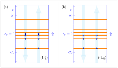
Figure 7: (color online) Lowest-energy eigenstates in two sectors of the even-$N$ particle-hole symmetric weak-coupling fixed-point Hamiltonian with $J_{\|}=u=V=0$. Panels (a) and (b) show the lowest many-body eigenstate in the $(q=1,s=1/2)$ and $(-1,1/2)$ sectors, respectively. The horizontal lines represent the single-particle energies resulting from the diagonalization of $H_{N}$, the blue spheres mark the filled levels, and the symbol $\Uparrow$ indicates the $z$ component of the magnon spin. Measured from the ground state, the many-body energies of both states are zero.

Figure 8 shows the two states at the corresponding strong-coupling fixed point. The magnon spin now being locked into a singlet with a holon, the remaining $N$ single-particle levels are symmetrically distributed around the Fermi level. The minimum-energy state in the $(1,1/2)$ [$(-1,1/2)$] sector contains a single particle (hole) at the lowest (highest) level above (below) the Fermi level. The two states are degenerate, with scaled energy $\hat{\eta}_{1+}=\hat{\eta}_{1-}$ relative to the ground-state energy. The energies $\hat{\eta}_{1\pm}$ are approximately described by Eq. (81), with $\delta=\pm\pi/2$. For $\Lambda=3$, in particular, $\hat{\eta}_{1\pm}=0.8$.

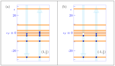
Figure 8: (color online) Lowest-energy eigenstates in two sectors of the even-$N$ particle-hole symmetric strong-coupling fixed-point Hamiltonian with $u=V=0$. Panel (a) shows the lowest many-body eigenstate at the $(q=1,s=1/2)$ sector, and panel (b) shows the lowest many-body eigenstate of the $(-1,1/2)$ sector. The horizontal lines are the single-particle energies resulting from the diagonalization of $H_{N}$, and the blue spheres indicate the filled levels. Measured from the ground state, in which all negative levels are filled, both states have scaled energy $\eta_{1}^{*}\approx 0.8$, for discretization parameter $\Lambda=3$.

The following sections describe the $N$ dependence of the lowest many-body energies in the $(\pm,1/2$) sectors for various model parameters. For subsequent reference, we start out with an example of particle-hole symmetry.

V.6.2 Particle-hole symmetric Hamiltonians ($u=V=0$)

With $u=V=0$, Equation (52) describes a particle-hole symmetric, anisotropic Kondo Hamiltonian, the renormalization-group trajectory of which has long been known to merge onto that of an isotropic Hamiltonian.Tsvelick and Wiegmann (1983) We therefore expect $H_{N}$ to flow from the vicinity of the particle-hole weak-coupling fixed point to the strong-coupling fixed point. Figure 9 shows an example, with $J_{\perp}=0.2v$ and $J_{\parallel}=0.01v$. The particle-like eigenstates in the $(1,1/2)$ sector are degenerate with the hole-like eigenstates in the $(-1,1/2)$ sector. The open circles depicting the lowest-energy eigenvalue of $H_{N}$ in the $(1,1/2)$ sector therefore coincide with the $+$ signs depicting the lowest-energy eigenvalue in the $(-1,1/2)$ sector as the Hamiltonian crosses over from near the weak-coupling fixed point to the strong-coupling fixed point. For comparison, the crossover for the isotropic model with $J_{\perp}=J_{\parallel}=0.2\,v$ is also shown. The inset shows that the crossover is universal, a horizontal shift $\Delta N=-9.1$ of the anisotropic curve being sufficient to make the two plots coincide.

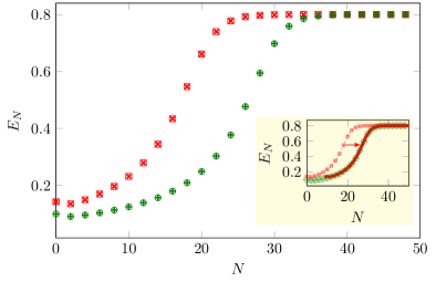
Figure 9: (color online) Scaled lowest energies $E_{N}$ as functions of iteration number $N$ for sectors $(1,1/2)$ (open circles) and $(-1,1/2)$ (crosses). The green circles and crosses represent eigenvalues of the Hamiltonian (V.4) with $u=V=0$, $J_{\perp}=0.2\,v$, and $J_{\parallel}=0.01\,v$. As $N$ grows, the renormalization-group transformation $\mathcal{T}[H_{N}]$ drives the Hamiltonian from the vicinity of the weak-coupling fixed point, where $E_{N}^{*}=0$, to the strong-coupling fixed point, where $E_{N}^{*}=0.8$. For comparison, the evolution of the eigenvalues for a symmetric Hamiltonian, with $J_{\parallel}=J_{\perp}=0.2\,v$, is also shown. The inset shows that, horizontally shifted by $\Delta{N}=9.1$, the isotropic curve (red solid line) coincides with the anisotropic curve (green crosses and open circles).

V.6.3 Particle-hole asymmetry

Figure 10 shows the $N$ dependence of the minimum energies in the $(1,1/2)$ and $(-1,1/2)$ sectors for $J_{\perp}=0.2\,v$, $J_{\parallel}=0.01\,v$, and $V=0.10\,v$, with $u=0$. The term proportional to $V$ on the right-hand side of Eq. (V.4) breaks the degeneracy between the $(1,1/2)$ and $(-1,1/2)$ energies and shifts the phases of the fixed-point single-particle levels, as discussed in Section V.2. The phase shifts at the weak-coupling fixed point affect the renormalization-group flow and delay the crossover to the strong-coupling fixed point. Universality is nonetheless preserved, as indicated by the congruence in the inset, which compares the isotropic curve in Fig. 9 with the two particle-hole asymmetric curves, both shifted horizontally by $\Delta N=-11.7$ and displaced vertically to insure agreement at large $N$.

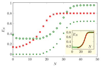
Figure 10: (color online) Scaled lowest energies in sectors $(\pm 1,1/2)$ as a function of iteration number for the indicated Hamiltonian parameters. As in Fig. 9, the corresponding energies for the isotropic, particle-hole symmetric Hamiltonian are shown for comparison. The symbol convention follows Fig. 9. The scattering potential $V$ breaks particle-hole symmetry and shifts the $(1,1/2)$ [$(-1,1/2)$] energies up (down). The crossover between the weak-coupling and the strong-coupling fixed points nonetheless follows the universal behavior in Fig. 9, as evidenced by the inset, which show the particle-hole symmetric, isotropic curve (red, solid line), horizontally displaced by $\Delta N=11.7$, and the asymmetric curves (green open circles and crosses) shifted vertically to make the large $N$ energies match the particle-hole symmetric fixed-point energies.

Figure 11 shows results for $u\neq 0$. The minimum energies in the $(\pm 1,1/2)$ sectors for $J_{\perp}=0.2\,v$, $J_{\parallel}=0.2\,v$, and $V=0.10\,v$, with $u=0.2\,v$ are plotted as functions of the iteration number $N$. Comparison with the flow in Fig. 10 show that the spin-dependent contribution to the bandwibandwidthdth, i. e., the term proportional to $u$ on the right-hand side of Eq. (V.4) perturbs two features of the renormalization-group flow: the weak-coupling (strong-coupling) phase shifts $\delta_{wc}$ ($\delta_{sc}$) is closer to its isotropic value $\delta_{wc}=0$ ($\delta_{sc}=\pi/2$), and the crossover from the weak-coupling to the strong-coupling fixed point is shifted to the right. The delayed crossover indicates that the operator $\mathcal{O}_{1}^{wc}$, defined in Sec. V.3, is less relevant. This conclusion agrees with Eq. (111), which shows that $u$ reduces $\delta(-)$ and increases $\delta(+)$ and therefore diminishes the difference $\mathrm{bar}\delta$, which controls the exponent on the right-hand side of Eq. (121). The $u$-dependent ground-state phase shifts and the universal crossover confirm that the term proportional to $u$ in the Hamiltonian is a marginal operator, which displaces the high-energy and the ground-state Hamiltonians along the lines of weak- and strong-coupling fixed points, respectively.

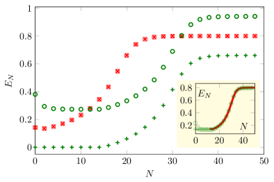
Figure 11: (color online) Scaled minimum energies in the sectors $(\pm 1,1/2)$ as functions of the iteration number for the indicated Hamiltonian parameters. We follow the symbol convention in Fig. 9 and for comparison reproduce the isotropic curve in Fig. 9. As in Fig. 10, the energies in the $(1,1/2)$ [$(-1,1/2)$] sector are shifted up (down) relative to the particle-hole symmetric energies. To show that universality is preserved, the inset shows the particle-hole symmetric curve (red, solid line) displaced horizontally by $\Delta N=12$, superimposed upon the particle-hole asymmetric curves (green, open circles and crosses) displaced vertically to insure agreement at the large $N$ limit.

Analogous results are obtained for other parametrical choices. In particular, as $u$ grows at fixed $J_{\perp}$, $J_{\parallel}$, and $V$, the crossover is displaced to progressively higher $N$, while the strong-coupling phase shifts $\delta_{sc}$ are slightly displaced to higher or lower values, chiefly depending on $V$. Figure 12 shows $\delta_{sc}$ as a function of the ratio $u/v$ for fixed $J_{\perp}=0.2v$ and illustrative choices of $J_{\|}$ and $V$. For $u=0$, we expect the weak-coupling phase shifts $\delta(\theta_{z})$ to be given by Eq. (121), and from the Friedel sum rule, expect the strong-coupling phase shift to differ from $\delta(\theta_{z})$ by $\pi/2$. We therefore expect $\delta_{sc}$ to obey the relation

$$\cot\delta_{sc}=-\pi\dfrac{V}{v},$$ (122)

which is approximately satisfied for all data in Fig. 12.

As $u$ grows, $\delta_{sc}$ diminishes for small $V$ and grows as $V$ exceeds $0.05v$. In all cases, however, $\delta_{sc}$ depends weakly on $u$ and is nearly independent of either $J_{\perp}$ or $J_{\|}$. Roughly speaking, therefore, the strong-coupling phase shifts are approximately described by Eq. (122) over the parametrical space of the Hamiltonian. Although the approximation distinguishing Eq. (V.4) from the scaled truncated Hamiltonian (V.1.3) restrict our analysis to small $u$, these results ratify the conclusion that the anomalous velocity is a marginal operator whose effect upon the physical properties of the system under study is limited to reducing the Kondo temperature and (slightly) displacing the low-temperature Hamiltonian along the line of strong-coupling fixed points.

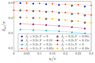
Figure 12: (color online) Strong-coupling fixed-point phase shifts as a function of the anomalous velocity $u$ at fixed $J_{\perp}=0.2\,v$, $J_{\parallel}=0.1\,v$, and $V=0.1\,v$. The phase shifts are obtained from Eq. (87), the single-particle energies $\eta_{m\pm}$ being identified as the limit to which the eigenvalue of the many-body state $g_{m}^{\dagger}$ ($m=2$) —sector $(1,1/2)$ tends as $N$ grows past the crossover. The isotropic limit of the phase shift, not shown, is $\delta/\pi=0.5$.

VI Conclusions

In this work, we considered the physics of doping a one-dimensional ferromagnetic insulator. Assuming spin-charge separation in the strongly interacting regime, we modelled the charge excitations by spinless fermions (holons) and the spin excitations by magnons.

The interaction between magnons and gapless holons in the limit of small doping gives rise to infrared singularities in perturbation theory. The mechanism behind these singularities is clarified by mapping to an effective field theory equivalent to an anisotropic Kondo model. In our case, the holons play the role of the conduction electrons and a magnon with momentum commensurate with the holon Fermi momentum $p_{F}$ plays the role of a mobile impurity. The internal degree of freedom of the impurity is a chirality pseudospin, which indicates whether the momentum is closest to $p_{F}$ or $-p_{F}$. A pseudospin flip corresponds to a $2p_{F}$ scattering process. Another difference from the conventional Kondo model is that the impurity (magnon) is mobile rather than localized. By applying a Galilean transformation to the frame moving with the magnon velocity $u$, we find that the effective Hamiltonian contains two holon bands with velocities $v+u$ or $v-u$ depending on whether the holons move in the same or opposite direction as the magnon.

We investigated the effects of the magnon-holon interaction in the nonperturbative, low-energy regime using the numerical renormalization group. We generalized the numerical method to treat the effects of a new marginal perturbation proportional to the magnon velocity $u$. The renormalization group flow takes the Hamiltonian from a line of weak-coupling fixed points characterized by two distinct phase shifts (related to scattering between the moving magnon and the two holon bands) to another line of strong-coupling fixed points with a single phase shift $\delta_{sc}$. The existence of only one phase shift can be interpreted in terms of the vanishing group velocity of the single-magnon excitation when the magnon momentum approaches $p_{F}$. By analogy with the original Kondo effect, we expect that at the strong-coupling fixed point the magnon pairs up with a holon to form a singlet of the chirality pseudospin. On the other hand, we should stress that, since the total magnetization is conserved, the real spin carried by the magnon is not screened. The residual potential scattering between the remaining holons and the magnon-holon pseudospin singlet accounts for the nonuniversal phase shift at the strong-coupling fixed point. Finally, we showed that the initial value of $u$ at the weak-coupling fixed point has a similar effect to the potential scattering term, namely it drives the phase shift away from the particle-hole symmetric value $\delta_{sc}=\pi/2$.

The results of this work suggest that it would be interesting to study dynamical response functions probing the spin excitation spectrum of one-dimensional itinerant ferromagnets when the magnon momentum approaches the holon Fermi momentum. In particular, the single phase shift $\delta_{sc}$ should have consequences for the power-law singularity at the single-magnon threshold in the transverse spin structure factor, which is equivalent to the magnon spectral function.Kamenev and Glazman (2009) Another interesting question is whether the Kondo effect discussed here can drive a nontrivial instability of the metallic ferromagnetic phase of a lattice model such as Tasaki’s model in Eq. (1), since it is expected to lower the energy of the single-magnon excitation. The behavior of the magnon spectral function in lattice models, such as Tasaki’s model in Eq. (1), could be investigated numerically using time-dependent density matrix renormalization group methods.White and Feiguin (2004); Schollwöck (2011)