Kenneth Wilson and lattice QCD

Abstract

We discuss the physics and computation of lattice QCD, a space-time lattice formulation of quantum chromodynamics, and Kenneth Wilson’s seminal role in its development. We start with the fundamental issue of confinement of quarks in the theory of the strong interactions, and discuss how lattice QCD provides a framework for understanding this phenomenon. A conceptual issue with lattice QCD is a conflict of space-time lattice with chiral symmetry of quarks. We discuss how this problem is resolved. Since lattice QCD is a non-linear quantum dynamical system with infinite degrees of freedom, quantities which are analytically calculable are limited. On the other hand, it provides an ideal case of massively parallel numerical computations. We review the long and distinguished history of parallel-architecture supercomputers designed and built for lattice QCD. We discuss algorithmic developments, in particular the difficulties posed by the fermionic nature of quarks, and their resolution. The triad of efforts toward better understanding of physics, better algorithms, and more powerful supercomputers have produced major breakthroughs in our understanding of the strong interactions. We review the salient results of this effort in understanding the hadron spectrum, the Cabibbo-Kobayashi-Maskawa matrix elements and CP violation, and quark-gluon plasma at high temperatures. We conclude with a brief summary and a future perspective.

1 Introduction

In early 1974, Kenneth Wilson circulated a preprint entitled ”Confinement of Quarks”. The paper was received by Physical Review D on 12 June 1974, and was published in the 15 October issue of that journal Wilson1974 . In this paper, Wilson formulated gauge theories on a space-time lattice. Using an expansion in inverse powers of the bare gauge coupling constant, Wilson demonstrated that lattice gauge theories at strong coupling confine charged states. He also argued that the absence of Lorentz invariance (or Euclidean invariance for the imaginary time used for the lattice formulation) is not a hindrance if there is a second order phase transition at some value of the gauge coupling constant, for in the vicinity of such a phase transition the lattice spacing can be taken to zero while fixing the physical correlation length at a finite value.

This paper laid the conceptual foundation for understanding the quark confinement phenomenon. It showed that large quantum fluctuations of gauge fields at strong coupling can generate a force between charged states which stays constant at arbitrary distances. This is a novel type of force, essentially different from the Yukawa force due to exchange of particles which tends to zero at large distances.

Initially, Wilson’s idea did not catch on rapidly. Techniques were hard to come by which allowed calculations of physical quantities such as hadron masses and connect them to physical predictions in the continuum space-time. The situation changed dramatically around 1979–1980 when Creutz, Jacobs and Rebbi CreutzJacobsRebbi1979 , and Wilson himself Wilson1979 , showed the possibility of numerically calculating the observables on a computer. Particularly dramatic was the calculation of the static quark-antiquark potential by Creutz for SU(2) gauge group in 1979 Creutz1979 , and the calculations in 1981 of hadron masses by Weingarten Weingarten1982 and by Hamber and Parisi HamberParisi1981 .

Traditional quantum field theory until that time could only deal with weakly coupled bound states such as hydrogen. The possibility of a technique which enables calculation of the properties of relativistic and strongly coupled bound states such as pion and proton was entirely new.

The timing was also perfect from computational point of view. The CRAY-1 supercomputer which appeared in 1976 had revolutionized scientific computing, and lattice QCD computation could quickly exploit vector supercomputers in the 80’s. Perhaps more important in retrospect, rapid development of microprocessors in the 70’s stimulated more than a few groups of particle theorists around the world to start developing parallel computers for lattice QCD.

The development of lattice QCD has been continuous since then. With large-scale numerical simulations on parallel supercomputers, understanding of physics of lattice QCD progressed, which in turn led to better algorithms for computation. These algorithms allowed a better exploitation of the next generation of more powerful computers, which brought even more progress of physics.

In the four decades of progress, lattice QCD has brought a deep understanding on the physics of the strong interactions. It has matured to the point where one can make calculations with the physical values of quark masses, on lattices with sufficiently large sizes, at lattice spacings small enough so that a continuum limit can be carried out with confidence.

In this article we review lattice QCD from four perspectives in the following four chapters. In Chapter 2, we discuss the foundation of lattice QCD, touching upon the connection between quantum field theory in Euclidean space time and statistical mechanics which was consciously exploited by Wilson. We show how it led to a conceptual breakthrough in the understanding of confinement. We also explain the issues related with chiral symmetry. In Chapter 3, we discuss the computational aspects. We review how lattice QCD embodies an ideal case of massively parallel computation, and how this led to the development of parallel supercomputers for lattice QCD, which impacted seriously on the history of supercomputers up to the present time. Also discussed is a special computational difficulty posed by the fermionic nature of quark fields, and how overcoming that difficulty has led to the algorithm in use today. In Chapter 4 we discuss some major physics results achieved so far in lattice QCD. The themes include the hadron mass spectrum, the determination of the Cabibbo-Kobayashi-Maskawa matrix and CP violation in the Standard Model, and the properties of quark gluon plasma at high temperatures and densities. Finally, in Chapter 5 we collect some thoughts on how Kenneth Wilson’s thinking and vision helped develop the subject.

The tone of this article is partly historical, describing the development of lattice QCD and the role Kenneth Wilson played in it. It also reviews the achievements made in the four decades since its inception in 1974.

2 Quantum chromodynamics on a space-time lattice

2.1 Hadrons, Quarks, Quantum Chromodynamics

If one looks up the Reviews of Particle Physics web page PDG , one finds there an entire list of particles and their properties experimentally discovered to date. In addition to “Gauge and Higgs Bosons”, “Leptons” and “Quarks”, there are two lists named “Mesons” and “Baryons”, each of which contains hundreds of particles. Protons and neutrons, which make up atomic nuclei, are two representative particles belonging to the family of baryons. Pions and K mesons are less familiar, but important particles for binding protons and neutrons into nuclei, and they belong to the family of mesons. The mesons and baryons are collectively called “hadrons”. Their chief characteristic is that they participate in the strong interactions in addition to the electromagnetic and weak interactions, while leptons participate only in the latter two interactions.

Many of hadrons were discovered in the accelerator experiments in the 50’s and 60’s. In 1964 Gell-Mann and Zweig proposed that hadrons are composed of more fundamental particles, which Gell-Mann named quarks. Quarks were predicted to have unusual properties such as fractional charge in units of electron charge. Evidence has gradually built up, however, that quarks are real entities. Yet experimental efforts for detecting them in isolation have been unsuccessful. This situation is often called “quark confinement”.

Quantum chromodynamics (QCD) proposes to explain the constitution of hadrons from quarks and their interactions. It is a quantum field theory with local SU(3) gauge invariance in which the quark field $q(x)$, with $x$ the space-time coordinate, transforms under the fundamental ${\bf 3}$ representation of SU(3). The SU(3) quantum numbers are called color since the basic premise of the theory is that only color neutral states, trivial under SU(3), carry finite energy and hence exist as physical states. This is a general statement of ”quark confinement”.

Local gauge invariance is a requirement that the frame of reference of an internal symmetry may be freely rotated at each space-time point without altering the content of the theory. Thus QCD as a gauge theory is to remain invariant under the transformation $q(x)\to V(x)q(x)$ where $V(x)\in{\rm SU(3)}$ may vary from point to point in space-time. This invariance requires the existence of a vector gluon field $A_{\mu}(x)$ with values in the Lie algebra of SU(3) which tells how the local frame at a point $x$ and at a different point $y$ are related.

QCD as field theory thus contains gluon as well as quark fields. It is defined by the Lagrangian density given by

$$\cal{L}_{\rm QCD} = \frac{1}{2g^{2}}{\rm Tr}\left(F_{\mu\nu}(x)^{2}\right)+\overline{q}(x)\left(i\gamma_{\mu}D_{\mu}+m\right)q(x).$$ (1)

Here, $q(x)=(q_{1}(x),\cdots,q_{N_{f}})$ is a spin 1/2 Dirac spinor field for quarks, $N_{f}$ denotes the number of quark flavors with $m=(m_{1},\cdots,m_{N_{f}})$ the quark mass matrix, and $D_{\mu}=\partial_{\mu}-iA_{\mu}(x)$ is the covariant derivative with $F_{\mu\nu}=\partial_{\mu}A_{\nu}-\partial_{\nu}A_{\mu}+[A_{\mu},A_{\nu}]$ the gluon field strength, and $g$ is the QCD coupling constant.

The discovery of asymptotic freedom GrossWilczek ; Politzer in 1974 showed that the coupling strength of non-Abelian gauge theories decreases toward zero at large momenta. Since deep inelastic electron nucleon scattering experiments carried out in the late 60’s indicated just such a behavior called scaling, the discovery boosted QCD to the leading candidate of the theory of strong interactions.

A beautiful prediction of asymptotic freedom is the existence of logarithmic violation of scaling which can be quantitatively calculated via renormalization group methods. The prediction was later confirmed by experiments, thus establishing the validity of QCD beyond doubt at high energies.

Since asymptotic freedom at high energies means that the coupling strength increases in the opposite limit of low energies, it was natural to speculate that QCD also provided a solution to the long standing puzzle that quarks had never been observed in experiments. However, quantum field theory at the time, though quite sophisticated, did not possess means to analyze the behavior of QCD for large coupling constant expected at low energies.

2.2 Formulation of QCD on a space-time lattice

An essential ingredient for a strong coupling analysis is a mathematically well-defined formulation of QCD in which ultraviolet divergences are controlled. Kenneth Wilson approached this problem with three key ideas: (i) use Euclidean space-time with imaginary time rather than Minkowski space-time with physical time, (ii) replace Euclidean space-time continuum by a discrete 4-dimensional lattice to control ultraviolet divergence, and (iii) maintain local gauge invariance as the guiding principle to construct field variables and action on the lattice.

The use of Euclidean space-time brings out a beautiful and powerful connection between quantum field theory and statistical mechanics. This connection was realized in the 60’s by Kurt Symanzik and others from the viewpoint of rigorously defining quantum field theory Symanzik1969 . The explosive development in the theory of critical phenomena due to Leo Kadanoff, Michael Fisher, Wilson himself and others in the late 60’s and early 70’s brought the importance of the concept to the foreground WilsonKogut1973 . A formal proof that quantum field theory in real time can be recovered from that in imaginary time under a set of axioms was given in the first half of 70’s OsterwalderSchrader1973 . This connection, then, was a hot topic at the time and Wilson consciously exploited it in his work on lattice QCD.

Let us consider a simple cubic 4-dimensional lattice in Euclidean space-time. The lattice points, called sites, are labeled by an integer component 4-vector $n=(n_{1},n_{2},n_{3},n_{4})\in{\bf Z}^{4}$, and have a physical coordinate $x=na$ with $a$ the lattice spacing. A pair of neighboring sites at $n$ and $n+\hat{\mu}$ with $\hat{\mu}$ the unit vector in the direction $\mu=1,2,3,4$ are connected by the link between the two sites which may be denoted as $\ell=(n,\mu),n\in{\bf Z}^{4},\mu=1,2,3,4$. An elementary square, or plaquette, on the lattice is then labelled by $P=(n,\mu,\nu)$ with $n$ the lowest corner and the two directions spanning the square denoted by $\mu$ and $\nu$. The lattice construction is illustrated in Fig. 1.

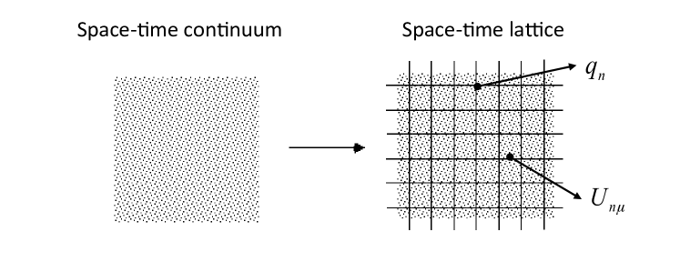
Figure 1: Replacing continuum space-time by a space-time lattice. Quark fields are placed at lattice sites, and gluon fields on links.

It is natural to place a quark field $q(x)$ on each site $q(x)=q_{n}$ with $x=na$. If one replaces the derivative $\partial_{\mu}q(x)$ by a finite difference $(q_{n+\hat{\mu}}-q_{n-\hat{\mu}})/2a$, the quark Lagrangian on a lattice will contain a bilocal term $\overline{q}_{n}q_{n\pm\hat{\mu}}$.

In the continuum space-time, bilocal quantities such as $\overline{q}(y)q(x)$ are rendered gauge invariant by inserting a path ordered phase factor $U(y,x)=P\exp(i\int_{x}^{y}A_{\mu}(x)dx_{\mu})$, which transforms as $U(y,x)\to V^{\dagger}(y)U(y,x)V(x)$ under the local gauge transformation. Wilson proposed to employ the phase factor along the lattice link $U_{n\mu}\sim P\exp(i\int_{na}^{(n+\hat{\mu})a}A_{\mu}(x)dx_{\mu})$ as the fundamental gluon field variable on the lattice. The lattice quark action can then be made invariant by inserting appropriate $U_{n\mu}$’s to the bilocal terms. One thus finds for the quark action on the lattice,

$$S_{\rm quark}=\frac{a^{3}}{2}\sum_{n\mu}\left(\overline{q}_{n}\gamma_{\mu}U_{n\mu}q_{n+\hat{\mu}}-\overline{q}_{n}\gamma_{\mu}U_{n-\hat{\mu}\,\mu}^{\dagger}q_{n-\hat{\mu}}\right)+a^{4}\sum_{n}\overline{q}_{n}m_{0}q_{n},$$ (2)

with $m_{0}$ the bare quark mass matrix.

A classical action for gluons which reduces to the continuum action in the limit $a\to 0$ can be constructed by taking the product of $U_{n\mu}$’s around the boundary of a plaquette $P$ Wilson1974 :

$$S_{\rm gluon} = \frac{1}{g_{0}^{2}}\sum_{P}{\rm Tr}\left[\prod_{n\mu\in\partial P}U_{n\mu}\right],$$ (3)

where ${\rm Tr}$ stands for trace over SU(3) indices. Here $g_{0}$ is the bare gauge coupling constant at the energy scale of the lattice cutoff $1/a$.

Lattice QCD as quantum theory is defined by the Feynman path integral. If $O(U,q,\overline{q})$ is an operator corresponding to some physical quantity, the vacuum expectation value over the quantum average is given by

$$\left<O(U,q,\overline{q})\right>=\frac{1}{Z_{\rm QCD}}\int\prod_{n\mu}dU_{n\mu}\int\prod_{n}d\overline{q}_{n}dq_{n}O(U,q,\overline{q})\exp(S_{\rm QCD})$$ (4)

with

$$Z_{\rm QCD}=\int\prod_{n\mu}dU_{n\mu}\int\prod_{n}d\overline{q}_{n}dq_{n}\exp(S_{\rm QCD}),$$ (5)

where

$$S_{\rm QCD}=S_{\rm gluon}+S_{\rm quark}.$$ (6)

The gluon link variable $U_{n\mu}$ takes values in the group SU(3) rather than the Lie algebra for the vector gluon field $A_{\mu}(x)$. The integration over $U_{n\mu}$’s should be defined as invariant integration over the group SU(3). Since SU(3) has a finite volume under this integration, the lattice Feynman path integral is well-defined without gauge fixing.

The integration over the quark fields also requires some care. Since quarks are fermions, the path integral has to be defined in terms of Grassmann numbers which anticommute under exchange, i.e., $q_{n}q_{m}=-q_{m}q_{n}$. These points are clearly spelled out in the Wilson’s original paper in 1974 Wilson1974 .

2.3 Confinement of color

Whether quarks are confined in QCD can be examined if one knows how to calculate the energy of an isolated quark in interaction with the gluon fields: an isolated quark would exist only if the energy of that state is finite. An elegant method invented by Wilson is to consider a pair of static quark and antiquark, which is created at some point in space-time, then separated to some distance, stays in that configuration for some time, and finally is brought together to a point and annihilated. Geometrically, the space-time trajectory of the pair forms an oriented closed loop $C$. Since the color charge of the quark interacts with gluon fields, the creation and annihilation of the pair inserts a phase factor

$$W\left[C\right]=P\exp\left(i\oint_{C}dx_{\mu}A_{\mu}(x)\right)$$ (7)

in the path integral where $P$ indicates ordering along the path. This is the Wilson loop operator.

If the loop has the shape of a rectangle of a width $R$ in the spatial direction and an extent $T$ in the temporal direction as shown in the left panel of Fig. 2, the quantum average of the Wilson loop operator measures the energy $E(R)$ of the quak-antiquark pair relative to the vacuum over a temporal length $T$ so that

$$\left<W\left[R\times T\right]\right>\propto\exp\left(-E(R)T\right),\quad T\to\infty.$$ (8)

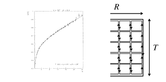
Figure 2: Left panel: Wilson loop for a temporal size $T$ and a spatial size $R$ measures the potential energy for a pair of static quark and antiquark. Right panel: The leading order of the strong coupling expansion is obtained by tiling the Wilson loop by plaquettes.

Wilson speculated that for large values of the gauge coupling, fluctuations of gluon fields would be large, leading to a significant cancellation among the contributions to the Wilson loop. This would mean that the Wilson loop average rapidly decreases for larger loops, or equivalently the probability decreases that the quark and antiquark are found in a well-separated configuration. This would mean confinement. Another equivalent statement would be that the energy $E(R)$ grows for larger separations $R$, so that separating quark from antiquark is not possible.

An amazingly simple calculation suffices to verify this picture if one employs lattice QCD. Let us assume, following Wilson, that quark fields do not play an essential role. When the bare coupling $g_{0}$ becomes large, the gluon path integral in (4) can be calculated by an expansion in inverse powers of $g_{0}^{2}$. The leading term is obtained when one tiles the $R\times T$ surface of the Wilson loop by a set of plaquettes from the expansion of the gluon part of the weight $\exp\left(S_{\rm gluon}\right)$, as shown in the right panel of Fig 2. We then find that

$$\left<W\left[R\times T\right]\right>=N_{c}\left(\frac{1}{N_{c}g_{0}^{2}}\right)^{RT/a^{2}}\left(1+O(g_{0}^{-8})\right),\quad g_{0}^{2}\to\infty,$$ (9)

with $N_{c}=3$ for SU(3) so that

$$E(R)\to\sigma R,\quad R\to\infty\quad{\rm with}\quad\sigma=\frac{1}{a^{2}}\left(\log\left(N_{c}g_{0}^{2}\right)+O(g_{0}^{-8})\right),$$ (10)

namely, a static pair of quark and antiquark are bound by a potential linearly rising with the separation. Hence they cannot be separated to infinite distance with any finite amount of energy.

A closed loop $C$ has two geometrical characteristics, the length of the loop $L[C]$ and the area of the minimal surface $A[C]$ spanned by the loop. The confinement behavior corresponds to an area decay for large loop;

$$\left<W\left[C\right]\right>\propto\exp\left(-\sigma A[C]\right).$$ (11)

If, on the other hand, the Wilson loop expectation value decays with the loop length,

$$\left<W\left[C\right]\right>\propto\exp\left(-\mu L[C]\right),$$ (12)

the energy of a quark-antiquark pair saturates to a constant $E(R)\to\mu$ for large separation $R\to\infty$. Hence there is no longer confinement. The confining and non-confining phases of gauge theories are thus distinguished by the behavior of the Wilson loop expectation value.

The possibility that there can be both confining and non-confining phases raises an interesting question whether a confining phase can turn into a non-confining phase if some parameters of the theory are varied. Temperature is such an important parameter. As we discuss in more detail in Sec. 4.4, the confining property becomes lost through a phase transition when the temperature is raised sufficiently.

2.4 Continuum limit

Let us go back to the strong coupling result in (10). If one uses the phenomenological value $\sqrt{\sigma}\approx 440{\rm MeV}$, and if one assumes that a value $\log\left(N_{c}g_{0}^{2}\right)\sim O(1)$ is sufficient for the strong coupling expansion to converge, the corresponding value of the lattice spacing equals $a\sim 0.5$ fm with 1 fm$=10^{-15}$ m. This value is comparable to a typical length scale of the strong interactions, e.g., the charge radius of proton $R_{p}\sim 0.9$ fm. We certainly know that space-time is continuous well below such length scales. Thus one need to know if confinement holds for smaller lattice spacings.

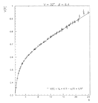
Figure 3: Monte Carlo result for the static potential energy $E(R)$ calculated in pure gluon theory showing a linearly rising term at long distances and a Coulomb term at short distances. From Ref. BaliShilling1993 .

In Fig. 3 we show the static potential $E(R)$ calculated by Monte Carlo simulation of the pure gluon theory BaliShilling1993 . We observe a linearly rising potential $E(R)\sim\sigma R$ at large distances. There is also a Coulomb behavior $V(R)\sim\alpha/R$ at short distances, which is consistent with a perturbative one gluon exchange expected from asymptotic freedom. The lattice spacing estimated from the phenomenological value $\sqrt{\sigma}\approx 440$ MeV is $a\approx 0.0544(4)$ fm. This is one of many evidences that the property of confinement holds not just at strong coupling but also toward weak couplings with small lattice spacings.

The question then is whether the confinement property really persists as the lattice spacing is taken toward the limit of continuous space-time $a\to 0$. For Wilson, who elucidated critical phenomena with his renormalization group ideas, this was not a conceptually difficult issue. The strong coupling calculation demonstrates that the system of gluons without quarks is in a confining phase. When one decreases the coupling constant $g_{0}$, this property persists as long as one does not encounter a phase transition to a non-confining phase characterized by perimeter decay (12). Suppose that there is such a second-order phase transition at $g_{0}^{2}=g_{c}^{2}$. Close to the critical point, the correlation length measured in lattice units diverges $\xi(g_{0})/a\to\infty$ as $g_{0}\to g_{c}$. This means that one should be able to hold the physical correlation length $\xi(g_{0})$ fixed to a physical value observed in experiment while sending the lattice spacing to zero $a\to 0$, recovering physics in the space-time continuum.

One can define lattice gauge theory for a variety of groups and space-time dimensions. As with the case for spin systems, the existence and position of second-order phase transition points would depend on them. For the group SU(3) in 4 dimensions, a particularly attractive possibility is $g_{c}=0$. In fact, this is the only possibility if confinement at low energies and asymptotic freedom at high energies are to coexist in the same phase.

The renormalization group allows a more concrete discussion. The change of gauge coupling $g_{0}\to g_{0}+dg_{0}$ under a change of cutoff scale $a\to a+da$ while fixing a physical scale constant defines a renormalization group $\beta$ function

$$a\frac{dg_{0}(a)}{da}=-\beta(g_{0}),$$ (13)

where the minus sign is inserted to be compatible with the conventional definition using momentum slicing. The strong coupling result (10) shows that $\beta(g_{0})$ is large and negative for large $g_{0}$. For small values of $g_{0}$, one can employ perturbation theory to confirm the asymptotic freedom result,

$$\beta(g_{0})=-b_{0}g_{0}^{3}-b_{1}g_{0}^{5}+O(g_{0}^{7})$$ (14)

with

$$b_{0} = \frac{1}{(4\pi)^{2}}\left(\frac{11}{3}N_{c}-\frac{2}{3}N_{f}\right),$$ (15)

$$b_{1} = \frac{1}{(4\pi)^{4}}\left(\frac{34}{3}N_{c}^{2}-\frac{N_{c}^{2}-1}{N_{c}}N_{f}-\frac{10}{3}N_{c}N_{f}\right),$$ (16)

for $SU(N_{c})$ gauge group and $N_{f}$ flavors of fermions in the fundamental representation. The first two coefficients are negative for our world with $N_{c}=3$ and $N_{f}=6$. A natural supposition is that the beta function is negative for all values of the coupling, with the only zero residing at $g_{c}=0$.

Wilson started a numerical Monte Carlo calculation to check this by a block spin renormalization group for gauge group SU(2) Wilson1979 . This attempt was followed by several serious calculations with SU(3) gauge group in the 80’s. The results, though mostly restricted to the pure gluon theory and had fairly large errors, showed that the beta function stayed negative and became consistent with the two-loop result (14) toward weak coupling (see, e.g., Refs. Bowleretal1986 ; Guptaetal1988 ).

Figure 4: Running of renormalized coupling constant $\alpha(q^{2})=g^{2}(q^{2})/4\pi$ in the Schrödinger functional scheme as a function of momenta scale $q$. Dashed and dotted lines are two- and one-loop evolution starting from the right-most point. The physical scale is fixed by the Sommer scale $r_{0}=0.5$ fm. From Ref. Luscheretal1994 .

A different, and perhaps a more elegant, approach was developed in the 90’s by the Alpha Collaboration Luscheretal1994 . Their method of step scaling function defines the renormalized coupling constant at a scale $1/L$ through the Schrödinger functional on a lattice of a finite size $L^{3}\times T$ with a prescribed boundary condition in time, and follows the evolution of the coupling under a change of scale by a factor 2. The continuum limit is systematically taken in this process. Therefore, the end result is the evolution of the renormalized coupling from low to high energies in the continuum theory.

In Fig. 4 we show the result for the pure gluon theory (solid circles) and a comparison with perturbation theory (dashed and dotted lines). The full evolution runs from 10 GeV down to a few hundred MeV, where the system is in a strong coupling non-perturbative regime. Thus the confining behavior at large distance is continuously connected with the asymptotically free behavior at short distances. The full evolution runs almost parallel to the two-loop evolution. Similar results have been obtained in full QCD with $N_{f}=2,3,4$ dynamical quarks ALpha2005 ; PACS-CS2009a ; AlphaNf4 .

Based on the results described above, one can state, though a mathematically rigorous proof is yet lacking, that QCD is in the confining phase over the entire range of coupling from zero to infinity.

2.5 Quarks and chiral symmetry

2.5.1 Chiral symmetry

An important feature of the strong interaction which was recognized in the late 50’s and early 60’s is chiral symmetry. Studies in this period led to the concept of spontaneous breakdown of symmetry, and a realization that it is accompanied by the emergence of massless bosons, called Nambu-Goldstone bosons today.

In QCD language, chiral symmetry is invariance under the global transformation $q(x)\to Wq(x)$, where $W=\exp(i\alpha\gamma_{5})\in{\rm SU(N_{f})}$ acts on the Dirac-flavor indices and rotates left and right handed chiral components of $q(x)$ in the opposite direction. This symmetry is explicitly broken by the quark mass term. Hence it holds approximately for three light quarks, up, down and strange. It is not very relevant for the heavier quarks, charm, bottom and top. The octet of pseudo scalar mesons, $\pi,K,\eta$, are identified as the Nambu-Goldstone bosons corresponding to spontaneous breakdown of chiral symmetry. With a strongly interacting dynamics at large distances, QCD should dynamically explain spontaneously broken chiral symmetry and its physical consequences.

2.5.2 chiral symmetry on a space-time lattice

Introduction of a space-time lattice affects bosons and fermions in different ways. This is most easily seen by looking at the kinetic term in the free field case. For a boson field $\phi_{n}$, the second-order derivative $-\partial_{\mu}^{2}\phi(x)$ is discretized as $-(\phi_{n+\hat{\mu}}+\phi_{n-\hat{\mu}}-2\phi_{n})/2a^{2}$, whereas for a fermion field $q(x)$, the first order derivative $\gamma_{\mu}\partial_{\mu}q(x)$ is discretized as $\gamma_{\mu}(q_{n+\hat{\mu}}-q_{n-\hat{\mu}})/2a$. The momentum space expression then becomes $2(1-\cos(p_{\mu}a))/a^{2}$ and $i\gamma_{\mu}\sin(p_{\mu}a)$, respectively. There is a crucial difference in the location of the zeros in the Brillouin zone: the boson case has a zero only at $p_{\mu}=0$ for all $\mu$ whereas the fermion case has a set of zeros for $p_{\mu}=0$ or $\pi/a$ for each $\mu$. Since the zeros gives rise to poles in the propagator, a naive fermion discretization leads to multiple copies of the state at $p_{\mu}=0$. This is the fermion species doubling problem.

Building upon a pioneering work by Karsten and Smit KarstenSmit1981 , Nielesen and Ninomiya NielsenNinomiya1981 proved that essentially the same conclusion holds under a set of rather general conditions. The theorem states that if the fermion action satisfies (i) chiral symmetry $q_{n}\to\exp(i\alpha\gamma_{5})q_{n}$, (ii) invariance under unit translation on the lattice, (iii) Hermiticity, and (iv) locality, then the spectrum of fermions contains even number of particles, half of them left handed and the other half right handed.

An elegant topological proof runs as follows karsten . If we write a Dirac fermion action on a lattice in a general form, $S_{F}=\sum_{n,m}\overline{q}_{n}D_{n,m}q_{m}$, the assumptions (i) and (ii) imply that $D_{n,m}=\sum_{\mu}\gamma_{\mu}F_{\mu}(n-m)$ where $F_{\mu}(n)$ is a vector function which, by (iii) satisfies $F_{\mu}^{\dagger}(n)=F_{\mu}(-n)$, and by (iv) rapidly decreases as $|n|$ becomes large. The Fourier transform $\tilde{F}_{\mu}(p)$ is, therefore, a well-defined real vector field over the Brillouin zone in momentum space. Let $p=p^{(i)},i=1,2,\cdots$ be the zeros of the vector field $\tilde{F}_{\mu}(p)=f_{\mu\nu}(p_{\nu}-p^{(i)}_{\nu})+O((p-p^{(i)})^{2})$. They correspond to the poles of the propagator $D^{-1}(p)$, and hence to the particle states. The relative chirality of these states are determined by the index, ${\rm sign}(\det f_{\mu\nu})$. Since the sum of index of a vector field over the 4-dimension torus vanishes by the Poincaré-Hopf theorem, there has to be an equal number of fermion states with opposite chirality.

The Nielsen-Ninomiya theorem indicates that one either has to abandon chiral symmetry or one has to allow for the presence of species doubling. Wilson’s choice, which he actually wrote down Wilson1975 prior to the publication of the theorem, was to add a term which softly breaks the chiral symmetry of the naive lattice action in (2):

$$\delta S_{\rm W} = \frac{a^{3}}{2}\sum_{n\mu}\left(2\overline{q}_{n}q_{n}-\overline{q}_{n}U_{n\mu}q_{n+\hat{\mu}}-\overline{q}_{n}U_{n-\hat{\mu},\mu}^{\dagger}q_{n-\hat{\mu}}\right).$$ (17)

For the free field case, this term adds $\sum_{\mu}(1-\cos p_{\mu}a)/a$ to the kinetic term $i\sum_{\mu}\gamma_{\mu}\sin p_{\mu}a$, and hence removes the zeros at $p_{\mu}=\pi/a$.

Let us add that toward the continuum limit $a\to 0$ the Wilson’s added term becomes of form $a\overline{q}(x)D_{\mu}^{2}q(x)$ relative to the original term $\overline{q}(x)i\gamma_{\mu}D_{\mu}q(x)$ in (2), i.e., higher order in $a$. Apart from removing the doublers, the effect of the added term disappears in the continuum limit.

Chiral breaking effects of the Wilson’s added term can be analyzed by the method of Ward identities Bochicchioetal1985 . In particular, a definition of quark mass can be given that satisfies the PCAC relation Bochicchioetal1985 ; ItohIwasakiOyanagiYoshie1986 . A detailed analysis of the phase structure on the $(g_{0},m_{0})$ plane was made Kawamoto1981 , and the existence of a massless pion, in spite of chiral symmetry breaking, was explained as due to spontaneous breakdown of parity Z(2) symmetry Aoki1984 . With these analytical developments, Wilson’s formulation provides a quantitative framework for the computation of physical observables, and is used extensively in Monte Carlo studies.

A variant of Wilson’s formulation is to consider two flavors of quarks as a pair and add a twisted mass term to the naive action (2) tmQCD2001 :

$$\delta S_{\rm tm}=a^{4}\sum_{n}\overline{q}_{n}i\mu_{q}\gamma_{5}\tau_{3}q_{n},$$ (18)

where $\tau_{3}$ acts on the flavor index. This formulation has an attractive feature that one can twist the angle $\alpha=\arctan\mu_{q}/m_{0}$ in such a way that $O(a)$ lattice artifacts are absent in physical observables tmQCD2004 ; AokiBaer2006 . Large-scale simulations are being made using such ”maximally” twisted QCD.

There is a different method, called the staggered formulation Susskind1977 , which retains a U(1) chiral symmetry at the cost of a four fold species doubling. In the 4-dimensional Euclidean formulation SharatchandraThusWeisz1981 , it starts with a single component fermion field $\chi_{n}$ at each site, and reconstructs four species of Dirac fields $\psi=(\psi_{1},\cdots,\psi_{4})$ from 16 $\chi$’s on the 16 vertices of a 4-dimensional unit hypercube KlubergSternetal1981 . The original action is invariant under an even-odd U(1) symmetry $\chi_{n}\to\exp(i(-1)^{|n|}\alpha)\chi_{n}$, which translates into an axial U(1) transformation on the four Dirac fields of form $\psi\to\exp(i\alpha\gamma_{5}\otimes\xi_{5})\psi$ where $\xi_{5}$ acts on the species index $\alpha$ of the Dirac field $\psi_{\alpha},\,\alpha=1,\cdots,4$.

It is generally believed that lattice QCD with the staggered fermion formalism converges to continuum QCD with $N_{f}=4$ degenerate flavors of quarks Sharpe2006 . An elaborate effective theory description has been developed to control the breaking of the full 4 ”flavor” chiral symmetry down to the U(1) subgroup at finite lattice spacing LeeSharpe1999 . On these theoretical bases, the staggered formalism is also extensively used in Monte Carlo simulations.

2.5.3 Lattice fermion action with chiral symmetry

In 1981, a year after Nielsen and Ninomiya presented their theorem, Wilson revisited the issue of chiral symmetry from a different perspective with Ginsparg Wilson1981 . He asked what would be the relation satisfied by a lattice Dirac operator $D_{n,m}$ if it were derived by a (chiral symmetry breaking) block spin transformation from a chiral invariant theory. The answer turned out to be remarkably simple; it is given by

$$\gamma_{5}D_{n,m}+D_{n,m}\gamma_{5}=a\sum_{k}D_{n,k}\gamma_{5}D_{k,m}.$$ (19)

Since $D$ does not anticommute with $\gamma_{5}$, assumption (i) of the Nielsen-Ninomiya theorem is not satisfied, and so the conclusion of the theorem does not hold. In fact, there is no species doubling. Furthermore, the axial vector current for this action has the correct U(1) anomaly.

One can rewrite (19) in terms of the propagator $G=D^{-1}$ as

$$\gamma_{5}G_{n,m}+G_{n,m}\gamma_{5}=a\delta_{nm}\gamma_{5}.$$ (20)

Hence the breaking of chiral symmetry is a local effect. One may expect then that a modified form of symmetry may exist. This was found almost 20 years later Luescher1998 . Fermion actions that satisfy the Ginzparg-Wilson relation (19) are invariant under an infinitesimal transformation given by

$$\delta\overline{\psi}=\overline{\psi}(1-\frac{1}{2}aD)\gamma_{5},\quad\delta\psi=\gamma_{5}(1-\frac{1}{2}aD)\psi.$$ (21)

Several forms of fermion action which satisfy the Ginsparg-Wilson relation were discovered in the 90’s. One form is a domain-wall formalism Kaplan1992 ; FurmanShamir1995 in which the 4-dimensional fermion field is constructed as the zero mode of a 5-dimensional theory generated by a mass defect at the boundary in a fictitious fifth dimension. Another form is given by the overlap formalism NarayananNeuberger1995 ; Neuberger1998 . In this case an explicit form of the operator $D$ is given by

$$D=\frac{1}{a}\left(1+\gamma_{5}H(H^{\dagger}H)^{-1/2}\right),\quad H=\gamma_{5}(aD_{W}-1)$$ (22)

with $aD_{W}+m_{0}$ the operator for the Wilson fermion action with a negative mass $m_{0}=-1$. The two forms are equivalent in the limit of infinite fifth dimension Neuberger1998-2 ; Borici1999 .

Yet another form is the perfect action HasenfratzNiedermeyer1998 , so named because it is defined as the fixed point of a block spin transformation of renormalization group for QCD. This form follows from the line of reasoning of Ginsparg and Wilson, but it was pursued and arrived at independently almost two decades later.

All forms of action, particularly the domain wall and overlap actions, have come to be used extensively in the last decade. The domain wall formalism has been exploited by RBC-UKQCD Collaborations (see, e.g., RBCUKQCDDomainwall2013 ), and the overlap formalism by JLQCD (see KEKOverlap2012 for a recent review). The situation with the perfect action is reported in Hasenfratzetal2005 .

2.5.4 Spontaneous breakdown of chiral symmetry

Spontaneous breakdown of chiral symmetry is best studied by examining the behavior of the order parameter of chiral symmetry. This is given by the quark bilinear operator $\Sigma=\left<\overline{q}_{n}q_{n}\right>$. If $\Sigma\neq 0$ after sending the spatial volume to infinity $V\to\infty$ followed by the limit of quark mass to zero $m_{q}\to 0$, then chiral symmetry is spontaneously broken.

In Fig. 5 we show the result for $\Sigma$ as a function of the degenerate up-down quark mass $m_{ud}$ in lattice units obtained with the overlap formulation for $N_{f}=2+1$ lattice QCD. We choose these data since the overlap formalism is the cleanest regarding the chiral aspect among lattice fermion formulations. The terminology $N_{f}=2+1$ refers to the fact that the up and down quark masses are taken degenerate, while the strange quark mass has a separate value. Strictly speaking, the values shown in Fig. 5 are obtained from the eigenvalue distribution of the Dirac operator and not by calculating the condensate directly.

The concave curvature as a function of $m_{ud}$ is consistent with the presence of a logarithm term predicted by chiral perturbation theory. Extrapolating to $m_{ud}=0$ including the effect of the logarithm yields a non-zero value, supporting spontaneous breakdown of chiral symmetry. The dependence of the pion mass is consistent with $m_{\pi}^{2}\propto m_{ud}$ (up to logarithmic corrections), as follows from the Nambu-Goldstone theorem.

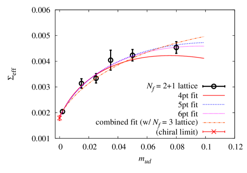
Figure 5: Chiral order parameter $\Sigma=\left<\overline{q}_{n}q_{n}\right>$ as a function of degenerate up-down quark mass in lattice units in $N_{f}=2+1$ flavor lattice QCD with overlap fermion formalism. The strange quark mass is held fixed at a value close to experiment. From Ref. KEKOverlap2012 . Color online.

Similar results have been obtained for the staggered fermion formalism which has U(1) chiral symmetry. The analysis is more complicated for the Wilson fermion formulation, since one needs to carry out a subtractive renormalization for both chiral condensate and quark mass due to the soft chiral symmetry breaking induced by the Wilson term (17). Once these subtractions are done, one finds the signatures expected for spontaneous breakdown of chiral symmetry, such as the relation $m_{\pi}^{2}\propto m_{ud}$ for an appropriately defined quark mass Bochicchioetal1985 ; ItohIwasakiOyanagiYoshie1986 .

2.6 Heavy quarks on a lattice

The three light quark quantum numbers, i.e., up, down and strange, have been known from 1930’s and 1950’s. In contrast, heavier quarks were discovered more recently, i.e., charm quark in 1974, bottom quark in 1977, and top quark in 1995. These heavy quarks occupied the central place in the experimental and theoretical studies toward establishing the Standard Model, particularly with the construction of B factories in the 90’s and experiments with them in the 2000’s.

Studying heavy quarks with lattice QCD poses the problem that for a large value of a heavy quark mass $m_{h}$, the dimensionless combination $m_{h}a$ is also large, leading to an amplification of lattice discretization errors, especially if $m_{h}a\gg 1$. This situation applies to the bottom quark with a mass $m_{b}\approx 5$ GeV, since lattice QCD simulations to date have been made with inverse lattice spacings in the range $a^{-1}\approx 2-4$ GeV.

Several methods have been formulated and employed to deal with this problem. The static approximation Eichten88 is an expansion in $1/m_{h}$, NRQCD LepageThacker88 is a reformulation of QCD for non-relativistic quarks with an expansion in powers of the quark velocity $v$, and a relativistic formalism ElKahdra1997 ; AokiKuramashi2003 ; ChristLin2007 modifies the Wilson quark action so as to systematically reduce the effects of large $m_{h}a$.

All three methods have been extensively used to calculate physical quantities involving charm or bottom quark. In particular, matrix elements such as the pseudoscalar decay constants and form factors calculated with these methods have been playing an important role in constraining the Cabibbo-Kobayashi-Maskawa matrix elements including the CP violation phase.

It should be mentioned that with increasingly smaller lattice spacings becoming accessible with progress of algorithms and computer power, direct simulations are replacing calculations with effective heavy quark theories. This has already occurred for charm quark, and it may not be too far into the future that bottom quark becomes treated in a similar way.

3 Lattice QCD as computation

3.1 Numerical simulation and lattice QCD

Lattice QCD offered a framework for conceptually understanding the dynamics of non-Abelian gauge fields. In particular, it elucidated the mechanism of confinement in a way which would have been impossible in the perturbative framework of field theory. Nonetheless, calculation methods to obtain physical results did not really exist; for example, higher order strong coupling expansions were very cumbersome and hard to extrapolate to the continuum limit expected at $g_{0}\to 0$.

Monte Carlo simulations offered a new approach to solve this impasse. Of course Monte Carlo methods had been known since the pioneering era of electronic computers in the late 40’ and early 50’s. The Metropolis algorithm to handle multi-dimensional integrations for statistical mechanical systems was formulated in 1953 Metropolis . Applications to spin systems in statistical mechanics started to appear in the 60’s and was pursued increasingly in the 70’s.

It is in this context that Creutz, Jacobs and Rebbi carried out a Monte Carlo study of Ising gauge theory with Z(2) gauge group in 4 dimensions in 1979, finding a first-order phase transition CreutzJacobsRebbi1979 . Creutz extended the application to SU(2) gauge group Creutz1979 , and extracted the string tension $\sigma$ in front of the area decay of the Wilson loop. The dependence of $\sigma$ on the gauge coupling $g_{0}$ turned out to be consistent with the scaling law predicted by the renormalization group. This suggested the possibility that a continuum limit could be successfully taken, giving rise to a hope that the confinement problem could be solved in a numerical way.

Wilson’s interest in numerical analyses and computer applications started early in his career Wilson2005 . He often used numerical methods to carry out his analyses. In his 1979 lecture at the Cargése Summer School Wilson1979 , Wilson reported a block-spin renormalization group analysis for SU(2) gauge group using Monte Carlo methods to evaluate the necessary path integral averages.

These attempts introduced a method hitherto unknown in field theory. The method looked very promising, and immediately attracted attention of particle theorists. In particular, it was applied to calculate masses of hadrons directly from quarks and gluons. The method was based on the observation that if $O_{\rm H}(t)$ is an operator at a time slice $t$ corresponding to a hadron H, e.g., $\pi^{+}\sim\overline{u}\gamma_{5}d$ for pion or $p\sim({}^{t}uC\gamma_{5}d)d$ for proton, then the 2-point Green’s function for this operator behaves for large times as

$$\left<O_{\rm H}(t)O_{\rm H}^{\dagger}(0)\right>\to Z\exp\left(-m_{\rm H}at\right),\quad t\to\infty,$$ (23)

where $m_{\rm H}$ denotes the mass of hadron H. Therefore, calculating the two-point function by a Monte Carlo simulation and extracting the slope of the exponential decay would yield the mass of hadron H.

This program was carried out by Weingarten Weingarten1982 , and by Hamber and Parisi HamberParisi1981 in 1981. The lattice size employed was $12^{4}$ for the Icosahedral subgroup of SU(2) for the former, and $6^{3}\times 12$ for SU(3) for the latter work. Albeit very modest in today’s standards, their studies clearly demonstrated the feasibility of their approach, which accelerated an explosive development of Monte Carlo simulations in lattice QCD.

3.2 Massive parallelism and lattice QCD

Monte Carlo simulation of lattice QCD is based on the method of importance sampling. Let $\phi_{n}$ be a field variable at a site $n$ on a lattice $\Lambda$ with $V$ lattice points, and $O(\phi)$ an operator. In field theory, one wishes to calculate the average value of $O(\phi)$ weighted with the action $S[\phi]$ according to,

$$\left<O(\phi)\right>=\frac{1}{Z}\int\prod_{n}d\phi_{n}O(\phi)\exp\left(S[\phi]\right),$$ (24)

where

$$Z=\int\prod_{n}d\phi_{n}O(\phi)\exp\left(S[\phi]\right).$$ (25)

Let us define a configuration $C$ as a point $C=(\phi_{1},\cdots,\phi_{V})$ in the integration space of all fields on the lattice $\Lambda$. Monte Carlo evaluation of the integral proceeds by setting up a stochastic chain of configurations $C_{1}\to C_{2}\to\cdots\to C_{N}$ such that the distribution of configurations converges to the weight of the integral:

$$\rho_{N}(C)=\frac{1}{N}\sum_{i=1}^{N}\delta(C-C_{i})\to\frac{\exp\left(S[C]\right)}{Z},\quad N\to\infty.$$ (26)

In the well-known Metropolis algorithm, the convergence is guaranteed by accepting or rejecting a new trial configuration $C_{\rm trial}$ according to the probability $P_{\rm acc}={\rm Min}\left(1,\exp(S[C_{\rm trial}]-S[C_{\rm old}])\right)$ where $C_{\rm old}$ is the latest configuration of the chain.

A very important property in Monte Carlo calculations of field theoretical systems is locality. A field variable $\phi_{n}$ at a site $n$ interacts only with those variables $\phi_{m}$’s in a limited neighborhood of the site $n$. In creating a trial configuration $C_{\rm trial}$ from an old configuration $C_{\rm old}$, and in calculating the difference of the action $S[C_{\rm trial}]-S[C_{\rm old}]$, the numerical operations at a site $n$ can be carried out independently of those at a site $m$ unless the pair is within the limited neighborhood of each other.

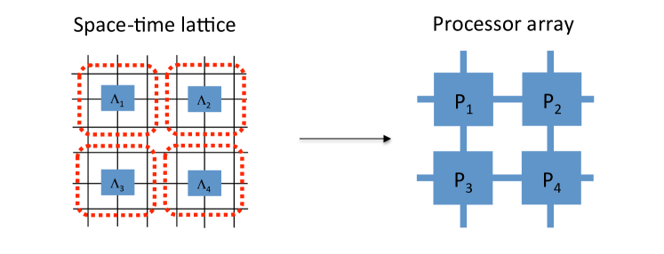
Figure 6: Mapping of space-time lattice $\Lambda=\cup_{\alpha=1}^{N_{P}}\Lambda_{\alpha}$ to an array of processors $P_{\alpha},\alpha=1,\cdots,N_{P}$ interconnected according to the space-time lattice topology. Color online.

As shown in Fig. 6, let us divide the entire lattice $\Lambda$ into a set of sub-lattices $\Lambda_{\alpha},\alpha=1,2,\cdots,N_{P}$, and assign each sub-lattice $\Lambda_{\alpha}$ to a processor $P_{\alpha}$. Because of locality, calculations by the processor $P_{\alpha}$ can be carried out independently of those by the other processors, except that the processors with overlapping boundaries have to exchange values of $\phi_{k}$’s in the boundaries before and/or after the calculations in each sub lattice. This means that, for a fixed lattice size, the computation time can be reduced by a factor $N_{P}$, and for a fixed sub-lattice size, one can enlarge the total lattice size proportionately to the number of processors $N_{P}$ without increasing the computation time.

This is an ideal case of the parallel computation paradigm. The locality property, which is one of the fundamental premises of field theoretic description of our universe, allows a mapping of calculations on a space-time lattice to a parallel array of processors interconnected with each other according to the connection of space-time sub-lattices.

3.3 Parallel computers for lattice QCD

Immediately after Monte Carlo calculations started in lattice QCD, several groups started to plan the building of a parallel computer for lattice QCD calculations. A crucial factor which helped push such an activity was a rapid development of microprocessors in the 70’s. As shown in Table 1, starting with a 4 bit Intel 4004 in 1971, increasingly more powerful microprocessors were developed and were put out on the market at prices affordable by academic scientific projects.

In Table 2 we list the parallel computers developed by physicists for lattice QCD in the 80’s. Typically, these machines employed a commercial microprocessor such as those listed in Table 1 as the control processor, and combined it with a floating point unit to enhance numerical computation capabilities.

Table 1: Representative microprocessors developed in the 70’s. Price/chip is from Wikipedia.

year	name	bit	price/chip
1971	Intel 4004	4 bit	$ 60
1972	Intel 8008	8 bit	$120
1974	Intel 8080	8 bit	$360
1974	Motorola 6800	8 bit	$360
1978	Intel 8086	16 bit	$320
1979	Motorola 68000	32 bit

Table 2: Parallel computers dedicated to lattice QCD developed in the 80’s. ”year” marks the completion date.

name	year	authors	CPU	FPU	peak speed
PAX-32*	1980	Hoshino-Kawai	M6800	AM9511	0.5 MFlops
Columbia	1984	Christ-Terrano	PDP11	TRW	–
Columbia-16	1985	Christ et al	Intel 80286	TRW	0.25 GFlops
APE1	1988	Cabibbo-Parisi	3081/E	Weitek	1 GFlops
Columbia-64	1987	Christ et al	Intel 80286	Weitek	1 GFlops
Columbia-256	1989	Christ et al	M68020	Weitek	16 GFlops
ACPMAPS	1991	Mackenzie et al	micro VAX	Weitek	5 Gflops
QCDPAX	1991	Iwasaki-Hoshino	M68020	LSI-logic	14 GFlops
GF11	1992	Weingarten	PC/AT	Weitek	11 GFlops
*not for lattice QCD

The famous CRAY-1 vector supercomputer came on the market in 1976. Vector supercomputers developed rapidly, and dominated the market in the 70’ and 80’s. However, the progress of parallel computers was even faster. By the end of the 80’s, parallel computers caught up and even overtook vector computers in speed. We can observe this trend by tracking blue and green symbols (vector computers) and red and violet symbols (parallel computers) from the 80’s to early 90’s in Fig. 7.

Table 3: Parallel computers developed for lattice QCD in the 90’s and later. ”year” marks the completion date.

name	year	authors	CPU	vendor	peak speed
APE100	1994	APE Collab.	custom	–	0.1Tflops
CP-PACS	1996	Iwasaki et al	PA-RISC	Hitachi(SR2201)	0.6TFlops
QCDSP	1998	Christ et al	TI DSP	–	0.6TFlops
APEmille	2000	APE Collab.	custom	–	0.8Tflops
QCDOC	2005	Christ et al	PPC-based	IBM(BG/L)	10TFlops
PACS-CS	2006	Ukawa et al	Intel Xeon	Hitachi	14TFlops
QCDCQ	2011	Christ et al	PPC-based	IBM(BG/Q)	500TFlops
QPACE	2012	Wettig et al	PowerXCell	–	200TFlops

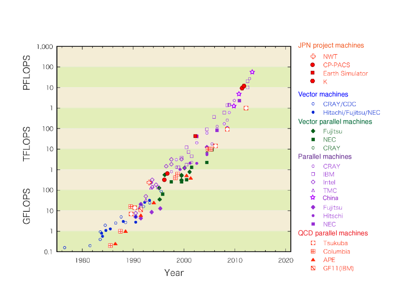
Figure 7: Peak speed of supercomputers. The circle at the bottom left is CRAY-1. Red fancy symbols show parallel machines developed for QCD. Color online.

In Table 3 we list the parallel computers developed in the 90’s and later for lattice QCD. Big success continued with CP-PACS in Japan, which occupied the top position in the Top 500 list of supercomputers in November 1996, and QCDSP in USA. We observe an increasing involvement of major vendors such as Hitachi and IBM. This was necessary to secure advanced technology and computer building knowhow to develop those fast computers. Probably the most well-known of this trend is the QCDOC project, which gave rise to the IBM BlueGene/L, and the QCDCQ project which ran parallel with the IBM BlueGene/Q development. In this way lattice QCD has seriously influenced the development of parallel supercomputers for scientific computing. Another trend one can observe in Table 3 is the use of commodity processors such as Intel Xeon for a quick machine building. This was the option adopted by PACS-CS and QPACE.

Today, the fastest supercomputers have reached the peak speed of $O(50)$ Pflops top500 . This has been achieved in two ways. The K computer in Japan and Sequoia (BlueGene/Q) in USA connected $O(10^{5})$ multi-core processors running at $O(100)$ Gflops. Tianhe-2 in China and Titan in USA boosted the computing power by adding multiples of GPGPU’s running at $O(1)$ Tflops to each node. Further increase of computing speed faces a serious issue that the memory cannot supply data fast enough to the processing units and the power consumption is becoming too large for large systems. Serious effort is already going on, however, to overcome these problems.

3.4 Fermion problem and hybrid Monte Carlo method

Monte Carlo calculation for the gluon fields, though somewhat complicated by the SU(3) nature of the field variable, is straightforward. Calculations for the quark fields, on the other hand, cannot be directly put on a computer since quark fields are represented by anticommuting Grassmann numbers. Instead one uses the identity 

$$\int\prod_{n}d\overline{q}_{n}dq_{n}\exp\left(\sum_{n,m}\overline{q}_{n}D_{n,m}(U)q_{m}\right)$$ (27)

$$= \int\prod_{n}d\phi^{\dagger}_{n}d\phi_{n}\exp\left(-\sum_{n,m}\phi^{\dagger}_{n}D^{-1}_{n,m}(U)\phi_{m}\right),$$ (28)

where $D$ represents the lattice Dirac operator and $\phi_{n}$ represents a bosonic field with 4 Dirac and 3 color indices to rewrite

$$Z_{\rm QCD}=\int\prod_{n\mu}dU_{n\mu}\int\prod_{n}d\phi^{\dagger}_{n}d\phi_{n}\exp\left(S_{\rm gluon}-\sum_{n,m}\phi^{\dagger}_{n}D^{-1}_{n,m}(U)\phi_{m}\right).$$ (29)

with which the fundamental variables $U_{n\mu}$’s and $\phi_{n}$’s are all bosonic.

The inverse $D^{-1}_{n,m}(U)$ is a non-local quantity. A change of a $\phi_{n}$ spreads across the lattice through the inverse. Therefore preparing a trial configuration whose acceptance can be controlled is not straightforward. A number of methods were developed in the 80’s including the micro canonical CallawayRahman1982 ; PolonyiWyld1983 and Langevin UkawaFukugita1985 methods. The latter was also explored by the group at Cornell including Wilson Wilson1985 . The standard method has settled on the hybrid Monte Carlo (HMC) method proposed in 1987 DuaneKennedyPendleton1987 , which we now discuss.

The first step of HMC is to introduce an SU(3)-algebra valued momentum $P_{n\mu}$ conjugate to $U_{n\mu}$, and rewrite the path integral (29) of full QCD as a partition function of a fictitious classical system of $U_{n\mu}$’s and $P_{n\mu}$’s as

$$Z_{\rm QCD}=\int\prod_{n\mu}dP_{n\mu}\prod_{n\mu}dU_{n\mu}\int\prod_{n}d\phi^{\dagger}_{n}d\phi_{n}\exp\left(-H\right),$$ (30)

where $H$ is a fictitious Hamiltonian defined by

$$H=\frac{1}{2}\sum_{n\mu}\mathrm{Tr}\left(P_{n\mu}^{2}\right)-S_{\rm gluon}(U)+\sum_{n,m}\phi^{\dagger}_{n}D^{-1}_{n,m}(U)\phi_{m}.$$ (31)

We now wish to generate a set of configurations distributed according to the weight $\exp(-H)/Z_{\rm QCD}$ by a Monte Carlo procedure. For this purpose, one introduces a fictitious time $\tau$ conjugate to the Hamiltonian $H$. Starting with a given configuration of $U_{n\mu}$ and $\phi_{n}$ at $\tau=0$, we solve Hamilton’s equations for the canonical pair,

$$\frac{d}{d\tau}U_{n_{\mu}} = iU_{n\mu}P_{n\mu},$$ (32)

$$\frac{d}{d\tau}P_{n\mu} = \frac{\partial}{\partial U_{n\mu}}S_{gluon}(U)$$ (33)

$$+ \sum_{n,k,l,m}\phi_{n}^{\dagger}D_{n,k}^{-1}(U)\frac{\partial}{\partial U_{n\mu}}D_{k,l}(U)D_{l,m}^{-1}(U)\phi_{m}$$

over some interval of $\tau$. The configuration at a final time $\tau$ is used as a new configuration in the Monte Carlo procedure.

In numerical implementations, a continuous fictitious time evolution is discretized with a finite step size $\delta\tau$. Since the Hamiltonian is no longer conserved, the configuration generated after a number of steps $\tau_{n}=n\delta\tau$ suffers from a bias. This is corrected by accepting or rejecting the generated configuration according to the Metropolis probability $P_{\rm acc}={\rm min}(1,\exp(-\delta H))$ where $\delta H=H(P(\tau_{n}),U(\tau_{n}))-H(P(0),U(0))$ is the difference of Hamiltonian over the trajectory of length $\tau_{n}=n\delta\tau$.

Hybrid Monte Carlo is an elegant method. It is (i) exact, (ii) allows control of acceptance, i.e., the probability that a trial configuration is accepted, through the magnitude of $\delta\tau$, and (iii) solving Hamltion’s equations can be executed in a parallel fashion. However, at every discretized step $\delta\tau$ in updating the fields according to the Hamilton’s equation, it requires the inverse of the lattice Dirac operator of form $x_{n}=\sum_{m}D_{n,m}^{-1}(U)\phi_{m}$ for given $U_{n\mu}$ and $\phi_{n}$.

The inverse can be obtained by solving the lattice Dirac equation,

$$\sum_{m}D_{n,m}(U)x_{m}=\phi_{n}.$$ (34)

This is a linear equation for a large but sparse matrix $D_{n,m}$, which can be obtained by iterative algorithms such as the conjugate gradient method. The number of iterations $N_{\rm iter}$ needed to reach an approximate solution is controlled by the condition number $\kappa(D)$ of the matrix $D$. It is given by $\kappa(D)=\lambda_{\rm max}/\lambda_{\rm min}$ where $\lambda_{\rm max}$ and $\lambda_{\rm min}$ are the maximum and minimum value of the eigenvalues of $D$. Typically, the iteration number $N_{\rm iter}$ is inversely proportional to the condition number. Since the minimum eigenvalue for the lattice Dirac operator is of the order of quark mass $m_{q}a$ in lattice units, and the maximum eigenvalue is $O(1)$, one finds $N_{\rm iter}\propto 1/m_{q}a$.

Among the six types of quarks known experimentally, the lightest up and down quarks have masses of the order of a few MeV. This is three orders of magnitude smaller than the typical hadronic scale of 1 GeV. The condition number of the lattice Dirac operator for these quarks is large, and therefore, hybrid Monte Carlo simulation slows down considerably as one tries to approach the physical values of quark masses.

3.5 Physical point calculation

Lattice QCD simulations including quark effects through hybrid Monte Carlo algorithm developed rapidly toward the end of the 90’s. By the turn of the century, there was enough experience accumulated to empirically estimate how much computing is needed to calculate observables with a quotable error for a given quark mass. In Fig. 8 is shown a typical plot Ukawa2001 , taking the case of $N_{f}=2$ flavor simulations for a lattice box of a size 3 fm, a minimum value to contain a hadron such as a nucleon within the box. The vertical axis shows the amount of computing in units of Tflops$\times$year, i. e., 1 year of running a computer executing 1 Tflop$=10^{12}$ floating point operations per second. The horizontal axis is the ratio of $\pi$ meson to $\rho$ meson masses, which varies with up and down quark masses and equals $m_{\pi}/m_{\rho}=0.18$ in experiment. The three curves correspond to the inverse lattice spacing $1/a=1,2,3$ GeV, with $1/a=2$ GeV or larger being needed for a reliable continuum extrapolation. We observe a sharp rise of the curves toward the physical value of $m_{\pi}/m_{\rho}=0.18$. This is a critical slowing down of the hybrid Monte Carlo algorithm, primarily arising from the slowdown of the Dirac solver toward $m_{q}a\to 0$.

Figure 8: Computational cost for generating 1000 independent configurations for $N_{f}=2$ flavor full QCD as a function of $m_{\pi}/m_{\rho}$ whose physical value equals $0.18$. The three curves correspond to the lattice spacing $a^{-1}=1,2,3$ GeV. Units is Tflops$\times$years, i.e., 1 year of time with the average speed of 1 Tflops. From Ref. Ukawa2001 .

The rapid increase presented a major problem for lattice QCD simulations. Without overcoming this problem, one could only compute at quark masses much heavier than the physical values. The results had to be extrapolated to the physical point, but such an extrapolation involved large systematic errors because of the existence of logarithmic terms of the form $\sim m_{q}\log m_{q}/\Lambda$ expected at vanishing quark mass.

The difficulty was resolved in the middle of the 2000’s Luescher2005 . Since the force in the Hamilton’s equation (33) involves $D^{-1}_{nm}(U)$, there are contributions coming from the short-distance neighborhood of the link $n\mu$ being updated and from those further away. It is possible to rewrite the quark determinant $\det D(U)$ such that these two types of contributions are separated. It was shown in Luescher2005 that, decomposing the lattice $\Lambda$ into a set of sub-lattices $\Lambda_{i},i=1,2,\cdots$, one can write

$$\det D(U)=\prod_{i}\det D_{i}(U)\cdot\det R(U),$$ (35)

where $D_{i}(U)$ is the Dirac operator restricted to a sub-lattice $\Lambda_{i}$ and $R$ couples sites belonging to different sub-lattices. Rewriting each determinant factor on the right hand side as a bosonic integral, one can write the force term as

$$F_{n\mu}=F_{n\mu}^{\rm gluon}+F_{n\mu}^{\rm UV}+F_{n\mu}^{\rm IR},$$ (36)

where $F_{n\mu}^{\rm gluon}$ is the term coming from the gluon action, $F_{n\mu}^{\rm UV}$ those arising from $D_{i}(U)$’s, and hence represents short-distance contributions, and $F_{n\mu}^{\rm IR}$ is the term from $R(U)$ giving long-distance contributions.

In Fig. 9 we show the magnitude of the three terms observed in a hybrid Monte Carlo run Luescher2005 . There is a clear separation of magnitude for the gluon, and UV and IR quark contributions. Therefore, the step size $\delta\tau_{\rm IR}$ for the IR part $F_{n\mu}^{\rm IR}$ can be taken much larger than $\delta\tau_{\rm UV}$ for the UV part, which in turn can be taken much larger than $\delta\tau_{\rm gluon}$ for the gluon part. An evolution with different step sizes for different parts of the force can be realized by a multi-time step integrator originally developed in SextonWeingarten .

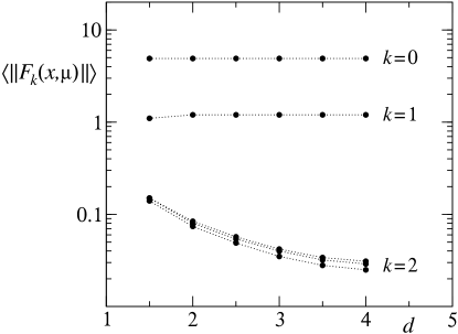
Figure 9: Magnitude of the force term $F_{n\mu}^{\rm gluon}(k=0)$, $F_{n\mu}^{\rm UV}(k=1)$, and $F_{n\mu}^{\rm IR}(k=2)$ as a function of distance from sub lattice boundary. From Ref. Luescher2005 .

Since inverting the long-distance part of the operator $R$ is the computationally most intensive, using different step sizes for the three parts of the force lead to acceleration of the evolution by a large factor of order $\delta\tau_{\rm IR}/\delta\tau_{\rm gluon}\approx 10-50$. Simulations incorporating such an acceleration technique were first carried out in the late 2000’s PACS-CS2009 , and reached the physical quark masses for the up and down quarks.

The separation of UV and IR parts of the quark force can be realized in a different manner Hasenbusch by rewriting the Dirac operator for a quark mass $m_{0}$ as a product of ratios of successively heavier masses,

$$D(U,m_{0})=\prod_{i=0}^{N}\left(D(U,m_{i})D^{-1}(U,m_{i+1})\right)\cdot D(U,m_{N}),$$ (37)

where $m_{i+1}$ is taken larger than $m_{i}$. Qualitatively speaking, one is separating the contributions to the force according to the eigenvalues in the range $[m_{i},m_{i+1}]$ with $m_{N+1}$ equal to the largest eigenvalue.

A somewhat different method to accelerate the hybrid Monte Carlo algorithm is provided by the rational hybrid Monte Carlo algorithm Horvathetal1999 . One writes

$$\det D=\left[\det D^{1/n}\right]^{n}=\int\prod_{i=1}^{n}d\phi^{i\dagger}d\phi^{i}\exp\left[-\sum_{i=1}^{n}\phi^{i\dagger}D^{-1/n}\phi^{i}\right]$$ (38)

for some positive integer $n$, and applies a rational approximation to the fractional power $x^{-1/n}$. If $\kappa$ is the condition number of $D$, the n-th root $D^{1/n}$ will have a smaller condition number $\kappa^{1/n}$. The magnitude of the force, compared with that of the hybrid Monte carlo method, will be reduced by a factor $\kappa^{1-1/n}$. Hence the step size can be increased by the corresponding factor, leading to an acceleration of the molecular dynamics evolution.

A final comment concerns the iterative inversion of the lattice Dirac operator (34). Since the increase of the number of iterations toward small quark masses is the cause of the slowdown of the hybrid Monte Carlo algorithm, an ultimate optimization of the algorithm would be realized if one could remove the critical slowdown. This has recently been achieved by understanding the modes corresponding to the small eigenvalues of the lattice Dirac operator. One can either construct these modes explicitly and ”deflate” (i.e., remove) them from the inversion Luescher2007 , or employ multi-grid techniques to adaptively generate and incorporate these modes in the inversion Babichietal2010 ; Frommeretal2013 .

Over the years, the improvements as described here plus the development of an increasingly powerful computers have made it possible to carry out lattice QCD calculations at the physical quark masses. Such calculations are now routinely done. This is an impressive achievement. It also carries an aesthetic appeal; with the physical quark masses, one is no longer simulating, but rather calculating, the physical processes of the strong interactions as they are taking place in our universe.

4 Physics results

4.1 Light Hadron spectrum

4.1.1 Mass spectrum of light mesons and baryons

Since the masses of hadrons are dynamical quantities, whether lattice QCD can quantitatively explain the experimentally known mass spectrum provides a stringent test of the validity of QCD at low energies. Furthermore, the success of such a calculation forms the basis on which the reliability of lattice QCD predictions of other physical quantities are to be built. For these reasons, the calculation of the hadron mass spectrum, in particular those of the ground states of light mesons and baryons composed of up, down, and strange quarks, has been pursued since the beginning of lattice QCD and numerical simulations.

A precise determination of the mass spectrum has to control a number of sources of errors. They are (i) statistical error due to the Monte Carlo nature of the calculation, (ii) systematic error due to extrapolation to the physical quark masses, (iii) systematic error due to finite lattice sizes, (iv) systematic error due to finite lattice spacings. In addition, until the late 90’s, most calculations were carried out with the so-called quenched approximation in which effects of quark-antiquark pair creation and annihilation are entirely ignored by dropping the quark determinant $\det D$ from the path integral. This was due to a high cost of including the quark effects into the simulations.

The first systematic attempt at a precision calculation of the light hadron spectrum was carried out by Weingarten and his colleagues within the quenched approximation in 1993 gf11 . The calculation took 1 year of dedicated computer time on GF11 computer developed by him at IBM. This was a landmark calculation in that a controlled extrapolation to the physical quark masses, to infinite volume and to zero lattice spacing, was systematically attempted. The masses of $\pi$, $\rho$ and $K$ mesons were employed to fix degenerate up and down, and strange quark masses. The masses of $K^{*}$ and $\phi$ for the meson octet, nucleon $N$ for the baryon octet, and $\Delta,\Sigma^{*},\Xi^{*}$ and $\Omega$ for the baryon decuplet were obtained as predictions. They are plotted by filled circles in the left panel of Fig. 10. The masses of $\Lambda,\Sigma$ and $\Xi$ of the baryon octet were not reported. The horizontal bars show the experimental values. We observe that the calculated values are consistent with experiment within one standard deviation. However, for baryons, a sizable magnitude of the errors of O(10$\%$) make it difficult to conclude if there is a precise agreement.

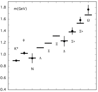
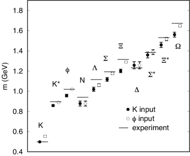
Figure 10: The left panel shows the result of the first systematic quenched light hadron mass spectrum calculation gf11 published in 1993. The right panel shows the definitive quenched result CP-PACS reported in 2000.

A definitive calculation of the hadron spectrum within the quenched calculation followed in 2000 CP-PACS . This work took half a year of CP-PACS computer which was 55 times faster than GF11. The results for the light meson and baryon ground states are shown in the right panel of Fig. 10. As one clearly sees there, the quenched spectrum systematically deviates from the experimental spectrum. If one uses the K meson mass $m_{K}$ as input to fix the strange quark mass (filled data points), the vector meson masses $m_{K^{*}}$ and $m_{\phi}$ are smaller by 4%($4\sigma$) and 6% ($5\sigma$), the octet baryon masses are smaller by 6% – 9% ($4-7\sigma$), and the decuplet mass splittings are smaller by 30% on average. Alternatively, if the $\phi$ meson mass $m_{\phi}$ is employed (open circles), $m_{K^{*}}$ agrees with experiment within 0.8% ($2\sigma$) and the discrepancies for baryon masses are much reduced. However, $m_{K}$ is larger by 11% ($6\sigma$). In other words, there is no way to match the entire spectrum beyond 5 to 10% precision in quenched QCD.

The CP-PACS calculation heralded the end of the era of quenched calculations. Efforts toward full QCD simulations, which had already been taking shape in the late 90’s, intensified. A first systematic calculation in full QCD was made by the CP-PACS Collaboration with dynamical up and down quarks ($N_{f}=2$) CP-PACS2000 . With the algorithmic development in the middle of the 2000’s, which we described in Sec. 3.5, calculations around the physical quark masses became possible. The PACS-CS Collaboration carried out $N_{f}=2+1$ flavor calculations in which the strange quark mass was taken close to the physical value and the pion mass was decreased down to $m_{\pi}=155$ MeV as compared to the physical value of 135 MeV PACS-CS2009 .

Finally, the BMW Collaboration carried out an infinite volume and continuum limit extrapolated calculation in 2008 BMW2008 . We reproduce their results in Fig. 11. There is good agreement with the experimental spectrum within the errors of 2–5% except for $\Delta$ for which the error is 13%.

Some of hadrons, including $\rho$ and $\Delta$, are resonances which decay for physical quark masses and infinite volume. A general relation between energy levels of two body states at finite volume and scattering phase shift, from which resonance parameters can be extracted, was established by Lüscher some time ago Luescher1991 . The BMW Collaboration assumed the Breit-Wigner form for the phase shift, and used this relation to correct the measured masses for the effects of decay coupling.

A more rigorous approach in which the phase shift is first extracted from measured energy levels and Lüscher’s formula, and resonance masses and widths are subsequently determined from the phase shift, was pioneered in Ishizuka2007 . Because of severe computational cost, it will take more time before physical point calculations can treat resonances numerically precisely in this way.

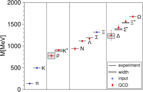
Figure 11: Light hadron mass spectrum in $N_{f}=2+1$ flavor QCD BMW2008 reported in 2008. Masses of $\pi$, $K$ and $\Xi$ are used to fix the degenerate up-down and strange quark masses as well as scale. Boxes of shaded grey show resonance masses and widths. Color online.

4.1.2 Isospin splittings of light hadron masses

The isospin multiplets of hadrons exhibit small mass differences of a few MeV. These tiny effects are nonetheless very important to understand our universe. For example, neutron with a mass $m_{n}=939.565379(21)$ MeV is heavier than proton of a mass $m_{p}=938.272046(21)$ MeV by $m_{n}-m_{p}=1.2933322(4)$ MeV. Because of this difference, neutron undergoes a $\beta$ decay with a mean life of $880.3(1.1)$ sec, which has important consequences in nucleosynthesis after the Big Bang, and the composition of nuclei as we see them today.

Since isospin mass splittings arise from the mass difference of up and down quarks, $N_{f}=1+1+1$ simulations with different masses for up, down, and strange quarks become necessary. Once we take the quark mass difference into account, one also likes to consider the electromagnetic effects, since the magnitude of the effect, expected at the order of a few MeV, is similar to those arising from the up-down quark mass difference.

A pioneering work on isospin breaking effects was carried out in the mid-90’s DuncanEichtenThacker1996 . The RBC Collaboration rekindled interest by pointing out its importance Blumetal2010 . Both quenched QED Blumetal2010 and full QED Ishikawaetal2012 ; PACS-CS2012 have been attempted. The most recent calculation has been reported by the BMW Collaboration BMW2014 . They carried out $N_{f}=1+1+1+1$ QCD and QED simulations with independent up, down, strange, and charm quark masses and three values of QED coupling for a variety of lattice sizes and spacings. A careful analysis of finite size effects due to the infinite range of photon was made. The infinite volume and continuum limit extrapolation was carried out. The final result is

$$m_{n}-m_{p}=+1.51(28){\rm~{}MeV}$$ (39)

in good agreement with experiment. Treating the hadron mass differences to first order in $m_{u}-m_{d}$ and QED coupling $\alpha$, they could separate QCD and QED contributions with the result,

$$m_{n}-m_{p}=+2.52(30)_{\rm QCD}-1.00(16)_{\rm QED}{\rm~{}MeV}.$$ (40)

There is a delicate cancellation between the QCD and QED effects before the final number settles on the experimental value.

4.2 Fundamental constants of the strong interaction

4.2.1 Quark masses

Table 4: Light quark masses in MeV units in the $\overline{\rm MS}$ scheme at $\mu=2$ GeV.

year		action	$\frac{m_{u}+m_{d}}{2}$	$m_{u}$	$m_{d}$	$m_{s}$
quenched QCD				1) $m_{K}$ input 2) $m_{\phi}$ input
2000	CP-PACS CP-PACS	Wilson	4.57(18)	–	–	115.6(2.3)1)
						143.7(5.8)2)
$N_{f}=2$ QCD				1) $m_{K}$ input 2) $m_{\phi}$ input
2000	CP-PACS CP-PACS2000	Wilson	$3.45^{+0.14}_{-0.20}$	–	–	$89^{+3}_{-6}$$\,\,{}^{1)}$
						$90^{+5}_{-10}$2)
$N_{f}=2+1$ QCD
2010	MILC MILC09	staggered	3.19(18)	1.96(14)	4.53(32)	89.0(4.8)
2010	BMW BMW2010	Wilson	3.469(67)	2.15(11)	4.79(14)	95.5(1.9)
2012	RBC/	domain	3.37(12)	–	–	92.3(2.3)
	UKQCD RBCUKQCDDomainwall2013	wall
Reviews of Particle Physics
1998	PDG PDG1998		2–6	1.5–5	3–9	60–170
2012	PDG PDG2012		$3.5^{+0.9}_{-0.2}$	$2.3^{+0.7}_{-0.5}$	$4.8^{+0.5}_{-0.3}$	$95\pm 5$

Table 5: Heavy quark masses in GeV units in the $\overline{\rm MS}$ scheme at $\mu=m_{h}$.

year		action	$m_{c}$	$m_{b}$	$m_{t}$
$N_{f}=2+1$ QCD
2010	HPQCD HPQCD2010	staggered	1.273(6)	4.164(27)	–
1998	PDG PDG1998		1.1–1.4	4.1–4.4	173.8(5.2)
2012	PDG PDG2012		1.275(25)	4.18(3)	173.07(89)

The determination of quark masses is a very important consequence of hadron mass spectrum calculations with lattice QCD. Since quarks are confined unlike leptons, lattice QCD provides the only reliable way for finding the values of this set of fundamental constants of our universe.

In Table 4 we list representative lattice results as well as estimates by Particle Data Group over the years. Even as late as 1998, the Review of Particle Physics listed quite a wide band of values as shown in this table. This exemplifies how uncertain quark masses were only a decade and a half ago. Two years later, the CP-PACS quenched spectrum calculation narrowed the range considerably. However, the limitation of quenched QCD is manifest in a large discrepancy of the strange quark mass depending on the input.

The $N_{f}=2$ full QCD calculation CP-PACS2000 including dynamical up and down quarks but treating strange quark in the quenched approximation showed that (i) quark masses are significantly smaller than indicated by the quenched results, and (ii) the discrepancy of strange quark mass depending on the input almost disappears.

The recent results from $N_{f}=2+1$ full QCD listed in Table 4 covers 3 types of fermion actions. All three calculations carry out infinite volume and continuum extrapolations, albeit the degree of sophistication differs among the three. The separate values of up and down quark masses are estimated using additional input on isospin breaking such as the $K^{0}-K^{+}$ mass difference and estimations on electromagnetic effects. The three sets of results are reasonably consistent. The 2012 Review of Particle Physics values reflect this progress.

In Table 5 we list the masses of charm and bottom quarks as determined by lattice QCD, together with those in Reviews of Particle Physics over the years. We also list the value for the top quark for completeness.

Lattice QCD is rapidly moving into the era when all three light quarks are treated independently, and dynamical effects of charm quark is also included. It will be soon that such calculations yield a direct calculation of each of the quark masses with a few % error.

4.2.2 Strong coupling constant

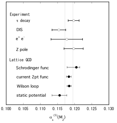
Figure 12: Strong coupling constant $\alpha_{s}^{(5)}(M_{Z})$ obtained from experiment and from lattice QCD. Here experiment means determinations from scattering and decay data combined with perturbative QCD. For further explanations, see text.

The value of the strong coupling constant $\alpha_{s}(\mu)=g^{2}(\mu)/4\pi$ defined in terms of the QCD coupling $g(\mu)$ at some prescribed scale $\mu$ is another fundamental constant of our universe, on a par with the fine structure constant $\alpha=e^{2}/4\pi$ for electromagnetism with the famous value $\alpha^{-1}=137.035999074(44)$.

In Fig 12 we plot the determinations obtained from scattering and decay data combined with perturbative QCD as of Fall 2013 PDG2013revision , and compare them with lattice QCD values from recent $N_{f}=2+1$ calculations. By convention, the scale is taken to be the Z boson mass $m_{Z}=91.1876(21)$ GeV, and five flavors of quarks excluding top is incorporated in the running of the coupling. Lattice QCD determinations employ experimental quantities at low energies such as hadron masses and decay constants for fixing the scale. The methods employed range from step scaling function using the Schrödinger functional by PACS-CS PACS-CS2009 , current 2-point function and Wilson loops by HPQCD HPQCD2010 , to static quark antiquark potential by Bazavov et al Bazavov2012 . The vertical band corresponds to the average over the four experimental determinations PDG2013revision , $\alpha_{s}^{(5)}(M_{Z})=0.1183(12)$.

The determinations with perturbative QCD still show some scatter and relatively large errors, and so do lattice QCD determinations depending on the method, the ones from current 2-point function and Wilson loops having the smallest error. There is consistency with experiment at 1% level, and the precision of lattice determinations will steadily improve.

4.3 CP violation in the Standard Model

4.3.1 CKM matrix elements

The connection between six types of quarks and CP violation is a salient feature of the Standard Model. The complex phase characterizing CP violation is encoded in the Cabibbo-Kobayashi-Maskawa matrix $V$ which appears in the weak interaction Lagrangian as

$$L_{int}=ig\left(\begin{array}[]{ccc}\overline{u},\overline{c},\overline{t}\end{array}\right)_{L}\gamma_{\mu}V\left(\begin{array}[]{c}d\\ s\\ b\end{array}\right)_{L}W_{\mu}^{-}+{\rm h.c.}$$ (45)

In the Wolfenstein parametrization, the matrix takes the form,

$$V=\left(\begin{array}[]{ccc}V_{ud},V_{us},V_{ub}\\ V_{cd},V_{cs},V_{cb}\\ V_{td},V_{ts},V_{tb}\\ \end{array}\right)=\left(\begin{array}[]{ccc}1-\lambda^{2}/2,\lambda,A\lambda^{3}(\rho-i\eta)\\ -\lambda,1-\lambda^{2}/2,A\lambda^{2}\\ A\lambda^{3}(1-\rho-i\eta),-A\lambda^{2},1\\ \end{array}\right)+O(\lambda^{4}),$$ (52)

with three real parameters $A,\lambda,\rho$ and an imaginary term $i\eta$ characterizing CP violation.

Constraining the CKM matrix requires matching experimental data on weak processes of hadrons to the theoretical expressions for the transition amplitudes which follow from the interaction Lagrangian above. Since quarks interact strongly according to QCD, the weak transition amplitudes are dressed by QCD corrections. These corrections can be calculated by lattice QCD.

One of weak processes which plays an important role is the CP violating mixing of neutral $K^{0}$ and $\overline{K}^{0}$ mesons. The experimentally measured state mixing amplitude $\epsilon$ can be written as

$$\epsilon=C\hat{B}_{K}\left\{\eta_{1}S(x_{c}){\rm Im}(\lambda_{c}^{2})+\eta_{2}S(x_{t}){\rm Im}(\lambda_{t}^{2})+2\eta_{3}S(x_{c},x_{t}){\rm Im}(\lambda_{c}\lambda_{t})\right\}.$$ (53)

Here $C$, $\eta_{1,2,3}$, $S(x,y)$, $S(x)=S(x,x)$ are known constants and functions, $x_{q}=m_{q}^{2}/m_{W}^{2}$ with $m_{q}$ and $m_{W}$ the mass of quark $q$ and W boson, and $\lambda_{q}=V_{qs}^{*}V_{qd}$ is the product of CKM matrix elements. The K meson bag parameter $B_{K}$ is defined as

$$B_{K}=\frac{\left<\overline{K}^{0}|\left(\overline{s}\gamma_{\mu}d\right)_{L}\left(\overline{s}\gamma_{\mu}d\right)_{L}|K^{0}\right>}{\frac{8}{3}f_{K}^{2}m_{K}^{2}},$$ (54)

where the expectation value is taken for QCD, and $\hat{B}_{K}$ is its renormalization group invariant value. We see then that the precision with which we can compute $B_{K}$ directly reflects in the precision in the determination of the CKM matrix elements through the products $\lambda_{q}=V_{qs}^{*}V_{qd}$.

Similarly, for the mixing of $B_{q}^{0}$ and $\overline{B}_{q}^{0}$ mesons with $q=d$ or $s$, the oscillation frequency $\Delta m_{q}$ is proportional to the $B_{q}$ meson decay constant $f_{B_{q}}$ and the bag parameter $B_{B_{q}}$ defined by

$$B_{B_{q}}=\frac{\left<\overline{B}^{0}|\left(\overline{b}\gamma_{\mu}q\right)_{L}\left(\overline{b}\gamma_{\mu}q\right)_{L}|B^{0}\right>}{\frac{8}{3}f_{B_{q}}^{2}m_{B_{q}}^{2}}.$$ (55)

In addition, the decays of $B$ mesons in the leptonic ($B\to\ell\nu$) and semi-leptonic (such as $B\to\pi\ell\nu$ and $B\to D^{*}\ell\nu$) channels are used to constrain the matrix elements $|V_{ub}|$ and $|V_{cb}|$.

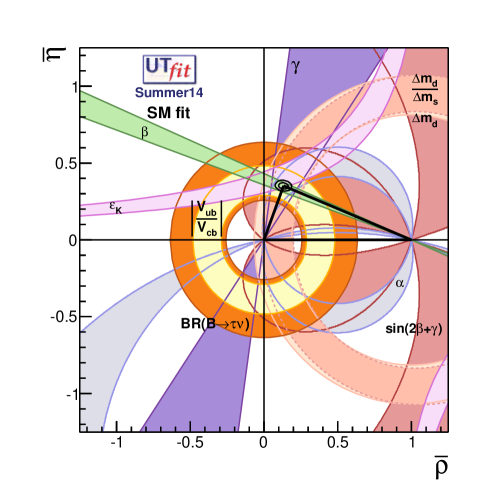
Figure 13: Latest constraints on the CKM matrix element expressed in the $(\overline{\rho},\overline{\eta})$ plane. From Ref. CKMfitter . Color online.

The constraint on the CKM matrix is usually written on the complex $(\overline{\rho},\overline{\eta})$ plane defined by

$$\overline{\rho}+i\overline{\eta}=\left(1-\frac{\lambda^{2}}{2}\right)\left(\rho+i\eta\right).$$ (56)

In Fig. 13 we show the latest result compiled by the UTfit Group UTfitter . The result by the CKMfitter group CKMfitter is similar. The inside of various regions are allowed from each of the constraints. There has to be a common overlap region if the Standard Model is to be consistent with experiment. Fitting data to the Standard Model, UTfit finds

$$\overline{\rho}=0.132(23),\quad\overline{\eta}=0.351(13).$$ (57)

Table 6: CP violating observables and relevant matrix elements. Percentage values of errors are also listed. See text for explanations.

observable	PDG PDG /		matrix	FLAG FLAG2014
	HFAG HFAG		element
$\epsilon$	$2.228(11)\times 10^{-3}$	0.49%	$\hat{B}_{K}$	0.7661(99)	1.3%
$\Delta m_{s}/\Delta m_{d}$	$34.8(2)$	0.60%	$\frac{f_{B_{s}}\sqrt{B_{B_{s}}}}{f_{B_{d}}\sqrt{B_{B_{d}}}}$	$1.268(63)$ FNAL2012	5.0%
${\cal B}(B\to\tau\nu)$	$1.14(27)\times 10^{-4}$	24%	$f_{B}({\rm MeV})$	$190.5(4.2)$	2.2%
${\cal B}(B\to\pi\ell\nu)^{1)}$	$0.38(2)\times 10^{-4}$	5%	$\Delta\zeta^{B\to\pi}$	2.16(50) HPQCD2006 ; FNAL2008	23%
$B\to D^{*}\ell\nu$	$35.85(45)\times 10^{-3}$	1.3%	$F^{B\to D^{*}}(1)$	0.906(13) FNAL2014	1.4%
1) integral over $16{\rm GeV}^{2}\leq q^{2}\leq q_{\rm max}^{2}$

For each region in Fig. 13 the width of the allowed band represents experimental uncertainties as well as those of lattice QCD determinations. In the two left columns of Table 6, we list the experimental inputs, and their percentage errors, used for constraining the allowed regions. The quantities and percentage errors listed in the two right columns are the QCD matrix elements which are needed to convert the experimental inputs to constraints in the $(\overline{\rho},\overline{\eta})$ plane.

The experimental values are taken from Reviews of Particle Physics PDG and a compilation of heavy flavor data by the Heavy Flavor Averaging Group HFAG . The lattice QCD values for hadronic matrix elements are taken from a recent compilation by the Flavor Lattice Averaging Group (FLAG) FLAG2014 . We select the values quoted for $N_{f}=2+1$ calculations that passes FLAG criteria for the control of systematics errors including the continuum extrapolation. In some cases, only a few calculations are available, in which cases we quote the original references.

We observe that B meson related quantities still has a significant margin for improvement, both on the experimental and lattice QCD sides. The SuperKEKB experiment, which will start in a few years, is expected to reduce the experimental error by another order of magnitude. Improvements in lattice QCD values should keep pace. We should also remark that the large error in the $B$ decay measurement affects the determination of $V_{cb}$, which in turn broadens the band for $\epsilon$. The determination of $B_{K}$ itself is already quite precise.

4.3.2 CP violation in the two pion decays of K meson

Historically, CP violation was discovered through an observation of K mesons decaying into two pions in 1964. The strength of direct CP violation relative to that in the state mixing is measured by the ratio

$$\frac{\epsilon^{\prime}}{\epsilon}=\frac{\omega}{\sqrt{2}|\epsilon|}\left[\frac{{\rm Im}A_{2}}{{\rm Re}A_{2}}-\frac{{\rm Im}A_{0}}{{\rm Re}A_{0}}\right],$$ (58)

where $A_{I}$ denotes the decay amplitude with isospin $I$ in the final state, and

$$\omega^{-1}=\frac{{\rm Re}A_{0}}{{\rm Re}A_{2}}.$$ (59)

Two heroic experiments, NA48 at CERN NA48 and KTEV at FNAL KTeV , spanning two decades from the 80’s to early 2000’s, measured $\epsilon^{\prime}/\epsilon$ with the result,

$$\frac{\epsilon^{\prime}}{\epsilon}=\left\{\begin{array}[]{ll}18.5(7.3)\times 10^{-4},&\quad{\rm NA48}\\ &\\ 20.7(2.8)\times 10^{-4},&\quad{\rm KTeV}\\ \end{array}\right.$$ (63)

It has also been a long standing puzzle that the amplitude for the $I=0$ final state is sizably larger than that for $I=2$, namely $\omega^{-1}\approx 22$. This is called the $\Delta I=1/2$ rule. Whether the Standard Model can successfully explain these features of $K\to 2\pi$ decay has been a major problem in particle physics. Since the issue boils down to calculating the strong interaction corrections to the effective weak interaction Hamiltonian, this has been an important challenge to lattice QCD since the 80’s.

There are three obstacles to a successful calculation of the $K\to\pi\pi$ amplitudes in lattice QCD. The first obstacle is chiral symmetry. Chirality plays an essential role in weak interactions. The effective 4-quark weak interaction Hamiltonian obtained at a lattice cutoff scale of a few GeV starting from a much higher weak interaction scale has a definite chiral structure Buras . Thus one has to employ a lattice fermion formulation which has chiral symmetry. If, on the other hand, one uses non-chiral formulations such as Wilson’s, one has to carefully control chiral symmetry violation effects under renormalization. The former option was not available until the late 90’s when domain-wall and overlap formulations were proposed. The latter problem was successfully resolved for the Wilson fermion action only recently, with an enticing conclusion that the renormalization structure is the same as in the continuum for $K\to\pi\pi$ decay Doninietal1999 ; Ishizuka2013 .

The second obstacle stems from the fact that, in the Euclidean Green’s function for the $K\to\pi\pi$ transition by the weak Hamiltonian, the two-pion state with zero relative momentum, being the state with lowest energy in this channel, dominates for large times. This contradicts the physical kinematics of the decay; the two pions decaying from a K meson at rest should have an equal and opposite momentum $p=\sqrt{m_{K}^{2}/4-m_{\pi}^{2}}$. Thus a naive calculation does not yield physical results. A resolution was found in 2001 LelloucheLuscher . One makes a calculation for a finite lattice volume chosen such that the energy of the two pion state matches the energy of the K meson. The physical amplitude for infinite volume can then be obtained by the following formula,

$$|A_{phys}(K\to\pi\pi)|^{2}=8\pi\frac{E_{\pi\pi}}{p}\left\{p\frac{d\delta_{\pi\pi}(p)}{dp}+q\frac{d\phi(q)}{dq}\right\}|\left<K|H_{W}|\pi\pi\right>_{lat}|^{2}.$$ (64)

Here $p$ is the pion momentum, $\delta_{\pi\pi}(p)$ the elastic $\pi\pi$ phase shift at momentum $p$, $q=pL/(2\pi)$, and $\phi(q)$ is defined by

$$\tan\phi(q)=-\frac{q\pi^{3/2}}{Z_{00}(1;q^{2})},\quad Z_{00}(1;q^{2})=\frac{1}{\sqrt{4\pi}}\sum_{\vec{n}\in Z^{3}}\frac{1}{\vec{n}^{2}-q^{2}}.$$ (65)

The third issue is specific to the $I=0$ channel and computational in character. In this channel, there are diagrams with disconnected quark loops, e.g., quarks from the pions annihilate themselves. In addition, the so-called Penguin diagrams in which a pair of quarks from the weak Hamiltonian forms a loop are also present. These diagrams suffer from large statistical fluctuations, rendering the statistical average difficult. This problem is gradually being overcome with efficient algorithms for computing disconnected and Penguin contributions, and with increase of computing power which allows a large number of Monte Carlo ensembles.

Recently there has been significant progress assembling these developments together. The RBC Collaboration has developed applications of the domain-wall formulation of QCD having chiral symmetry. It has succeeded in calculating the $I=2$ amplitude for the physical pion mass RBRC2012 . Their result, obtained at a lattice spacing of $a\approx 0.14$ fm, is given by

$${\rm Re}A_{2} = +1.381(46)_{\rm stat}(258)_{\rm syst}\times 10^{-8}{\rm GeV},$$ (66)

$${\rm Im}A_{2} = -6.54(46)_{\rm stat}(120)_{\rm syst}\times 10^{-13}{\rm GeV}.$$ (67)

The real part is in good agreement with experiment: ${\rm Re}A_{2}^{\rm exp}=1.479(4)\times 10^{-8}$ GeV.

The RBC Collaboration has been attacking the much more difficult $I=0$ channel, using a special $G$-periodic boundary condition to force the pions to carry momentum so that an energy matching is realized between the K meson and 2 pions. Preliminary results have been presented at Lattice 2014 Conference this year.

Another group at Tsukuba has been pursuing the problem using the Wilson fermion formulation Ishizuka2013 . The renormalization structure for the operator relevant for $K\to\pi\pi$ decay turned out to be the same as in the continuum except for the mixing with dimension 3 operator $\overline{s}\gamma_{5}d$, which is subtracted non-perturbatively. Their calculation so far does not achieve physical kinematics. The $\pi$ meson mass is artificially taken large so that $2m_{\pi}=m_{K}$ is satisfied. Nonetheless they reported an encouraging first result for $I=0$ channel as well as for $I=2$ at Lattice 2014 Conference.

It is hoped that progress in the near future brings definitive results on the $I=0$ amplitude $A_{0}$. This will put an independent constraint on the CP violating phase $\bar{\eta}$ in Fig. 13 as the ratio $\epsilon^{\prime}/\epsilon$ is proportional to $\bar{\eta}$.

4.4 Quark-gluon matter at high temperature and density

Confinement of quarks and spontaneous breakdown of chiral symmetry are both dynamical consequences of QCD. A very interesting question then is how these properties may or may not change if parameters (or dials) external to QCD are varied. One of important dials is temperature, which increases toward the Big Bang in the Early Universe. Another dial is baryon number density, which has a large value in extreme conditions such as in the core of neutron stars.

In both cases one is interested in an aggregate of hadrons, rather than individual hadrons, and wants to understand how its properties change at extremely high temperature or density. As we discuss below, a general conclusion from lattice studies is that a gas of hadrons turns into a different state in which quark and gluon degrees of freedom becomes manifest. The novel state of matter is often called quark-gluon plasma (QGP).

4.4.1 Phase diagram of QCD at finite temperature:analytical considerations

The Euclidean formulation adopted for lattice QCD is well suited for studies of its properties at finite temperatures. If one considers a lattice with $N_{t}$ sites in the temporal direction, and imposes periodic and antiperiodic boundary condition for gluon and quark fields, respectively, the lattice path integral (5) is equal to the canonical partition function

$$Z_{\rm QCD}={\rm Tr}\left[\exp\left(-H_{\rm QCD}/T\right)\right],$$ (68)

at a physical temperature

$$T=\frac{1}{N_{t}a}.$$ (69)

This connection shows that methods developed for zero temperature studies, including Monte Carlo calculations, are readily applicable to the finite temperature case.

In order to discuss what happens as the temperature is raised from zero, it is helpful to consider a two-dimensional plane of the average up-down quark mass $m_{ud}$ and the strange quark mass $m_{s}$, often dubbed Columbia Plot, as depicted in Fig. 14 Columbia1990 . One can examine various limiting cases as follows.

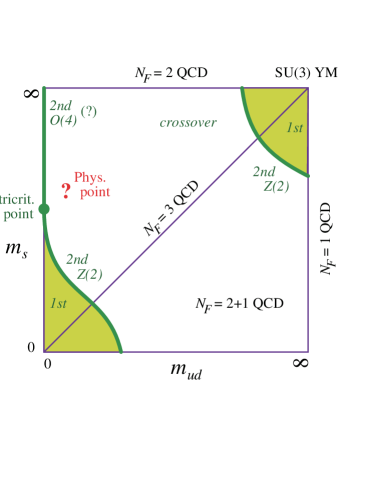
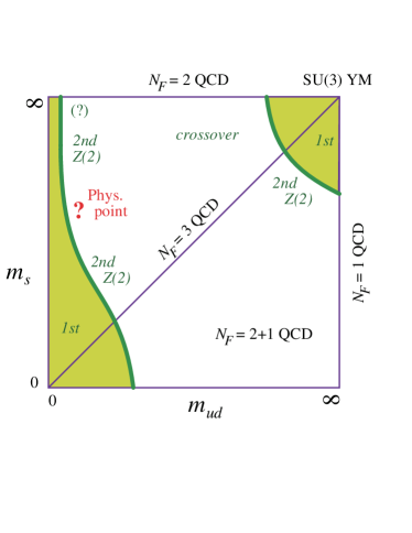
Figure 14: Phase digram in 2+1 flavor QCD as a function of the degenerate $u$ and $d$ quark mass $m_{ud}$ and the $s$ quark mass $m_{s}$. Left panel shows the case for a second order chiral transition for two-flavor QCD. Right panel shows the case for a first order two-flavor chiral transition. From Ref. Kanaya2010 . Color online.

(i) Pure gluon theory:

The top right corner in Fig. 14 for $m_{ud}=m_{s}=\infty$ corresponds to the pure gluon theory without quark degrees of freedom. This case is important, nonetheless, since confinement is a dynamical consequence of the gluon fields.

The pure gluon theory possesses a center $Z(3)$ symmetry defined by the transformation

$$U_{n4}\to\zeta U_{n4},\quad\zeta\in Z(3),$$ (70)

for the sites $n$ on some fixed time slice $t$. The corresponding order parameter is the Wilson loop winding around the space-time in the time direction at a fixed spatial site $\vec{n}$ defined by

$$\Omega(\vec{n})={\rm Tr}\left(\prod_{n_{t}=1}^{N_{t}}U_{(\vec{n},n_{t})4}\right).$$ (71)

This operator, often called Polyakov loop, transforms under the center Z(3) symmetry as

$$\Omega(\vec{n})\to\zeta\Omega(\vec{n}).$$ (72)

PolyakovPolyakov and Susskind Susskind argued that the center Z(3) symmetry is intact at low temperatures with $\left<\Omega(\vec{n})\right>=0$, but becomes spontaneously broken beyond a certain temperature $T=T_{c}$ with a non-zero expectation value $\left<\Omega(\vec{n})\right>\neq 0$.

The connection with deconfinement is most easily understood in the following way. The 2-point correlation function of Polyakov loops defined by $\left<\Omega(\vec{n})\Omega^{\dagger}(\vec{m})\right>$ is connected with the free energy $F(|\vec{n}-\vec{m}|)$ of a static quark at site $\vec{n}$ and an antiquark at site $\vec{m}$ by

$$\exp\left(-F(r)/T\right)=\left<\Omega(\vec{n})\Omega^{\dagger}(\vec{m})\right>,\quad r=|\vec{n}-\vec{m}|.$$ (73)

Assuming the presence of a mass gap $\mu$, the 2-point function on the right hand side is expected to behave for large $r$ as

$$\left<\Omega(\vec{n})\Omega^{\dagger}(\vec{m})\right>\to\left<\Omega(\vec{n})\right>\cdot\left<\Omega^{\dagger}(\vec{m})\right>+O\left(\exp\left(-\mu r\right)\right),\quad r\to\infty.$$ (74)

Depending on the expectation value $\left<\Omega\right>$, one finds for $r\to\infty$ that

$$F(r) \to \left\{\begin{array}[]{ll}\sigma r,&\quad\left<\Omega\right>=0,\quad T<T_{c}\\ &\\ c+O(\exp\left(-\mu_{D}r\right)),&\quad\left<\Omega\right>\neq 0,\quad T>T_{c}\\ \end{array}\right.$$ (78)

where $\sigma=T\mu$ for $T<T_{c}$, and $c$ is a constant and $\mu_{D}=\mu$ is a color electric Debye screening mass for $T>T_{c}$.

Analytical considerations indicate that this deconfinement phase transition should be of first order YaffeSvetitsky . If this is the case, the first-order transition will extend into the region of large but finite quark masses BanksUkawa , terminating at a line of second-order transition as depicted in Fig. 14.

(ii) $N_{f}=2$ and $N_{f}=3$ massless QCD:

The top left corner of Fig. 14 corresponds to $N_{f}=2$ massless QCD with $m_{ud}=0$ but $m_{s}=\infty$, and the bottom left corner to $N_{f}=3$ massless QCD with $m_{ud}=0$ and $m_{s}=0$.

For $N_{f}$ flavors of massless quarks, QCD is invariant under a global $SU(N_{f})\otimes SU(N_{f})$ chiral symmetry, which is spontaneously broken down to vector $SU(N_{f})$ symmetry with a non-zero vacuum expectation value of the order parameter $\Sigma=\left<\overline{q}_{n}q_{n}\right>\neq 0$. The $N_{f}^{2}-1$-plet of pseudo scalar mesons are the corresponding Nambu-Goldstone bosons.

When one raises the temperature, thermal fluctuations tend to destabilize the chiral order parameter $\Sigma$. Thus one expects a phase transition restoring chiral symmetry at some temperature. A more detailed examination is possible using an effective non-linear sigma model for the order parameter field $\Phi_{n}^{ij}=\overline{q}_{n}^{i}q_{n}^{j}$ with $i,j=1,\cdots,N_{f}$ and renormalization group methods. The result PisarskiWilczek indicates that (i) for $N_{f}=3$ or larger, chiral symmetry is restored through a first order phase transition, while (ii) for $N_{f}=2$ the phase transition is of first or of second order depending on whether flavor singlet $U(1)$ axial symmetry is effectively restored or not at $T>T_{c}$.

(iii) Connecting $N_{f}=2$ and $N_{f}=3$ massless QCD:

One can interpolate between the $N_{f}=2$ and $3$ cases by changing the strange quark mass $m_{s}$ from $\infty$ to $0$. If the $N_{f}=2$ transition is of second order, the first order transition for $N_{f}=3$ at $m_{s}=0$ has to change to a second order transition at a tricritical point at some $m_{s}=m_{s}^{c}$.

(iv) $N_{f}=3$ symmetric QCD:

In general, a first order phase transition is stable under symmetry breaking perturbations up to a critical value where it terminates with a second order phase transition. For the second order case, the phase transition immediately disappears if symmetry breaking perturbations are turned on. Thus one expects a sheet of first order transition extending from the bottom left corner corresponding to $N_{f}=3$ massless QCD to the interior of the phase diagram. The sheet should terminate at a line of second order phase transitions, which is expected to belong to the Ising universality class GavinGokschPisarski .

If the $N_{f}=2$ transition at $m_{ud}=0$ is of second order, this line of second order transitions will hit the vertical axis at $m_{s}=m_{s}^{c}$ with a power law $m_{ud}\propto(m_{s}^{c}-m_{s})^{5/2}$ Rjagopal1995 , as depicted in the left panel of Fig. 14. If, on the other hand, the $N_{f}=2$ transition is of first order, the line will go up to the top horizontal line (the right panel of Fig. 14).

4.4.2 Monte Carlo study of the finite-temperature phase diagram

Lattice QCD simulations are carried out for a fixed temporal lattice size $N_{t}$. One then regulates the temperature indirectly by varying the bare gauge coupling constant $g_{0}^{2}$; since the continuum limit $a=0$ is located at $g_{0}^{2}=0$, weaker couplings correspond to smaller lattice spacing, and hence to higher temperatures, and vice versa for stronger couplings and to lower temperatures.

The basic tool for studying the phase diagram is finite size scaling theory developed in the late 60’s and 70’s FSS . This theory helps to analyze how singularities marking phase transitions develop from numerical data obtained at finite volumes.

(i) Pure gluon theory:

The first instance where finite size scaling method was crucially effective was the deconfinment transition of the pure gluon theory. Early simulations quickly found that the Polyakov loop expectation value exhibited a rapid increase from $\left<\Omega\right>\approx 0$ to non-zero values over a narrow range of temperature as expected. A subtle issue is if a rapid increase actually signifies a phase transition, and if so, whether it is a first order phase transition with a discontinuous jump of $\left<\Omega\right>$ at $T_{c}$ or a second order phase transition with a continuous $\left<\Omega\right>$ but having a singular derivative.

The susceptibility of Polyakov loop is defined by

$$\chi_{\Omega}=\frac{1}{L^{d}}\sum_{\vec{n},\vec{m}}\left<\Omega(\vec{n})\Omega^{\dagger}(\vec{m})\right>$$ (79)

with $L$ the linear extent of the system, and $d$ the space dimension. For a finite volume, the susceptibility exhibits a peak. The infinite behavior of the peak height $\chi_{\Omega}^{\rm max}$ distinguishes the order of the phase transition. According to finite size scaling theory, if one parametrizes the volume dependence by a power law,

$$\chi_{\Omega}^{\rm max}(L)\propto L^{\alpha},\quad L\to\infty,$$ (80)

the value $\alpha=d$, i.e., the dimensionality of space, signals a first order transition, while values $\alpha<d$ characterizes a second order transition in which case $\alpha$ is related to the critical exponents. Similar criterion holds for the volume dependence of the width of the peak.

These criteria were utilized to establish the first order nature of the deconfinement transition in the pure gluon theory FukugitaOkawaUkawa , in agreement with the analytical considerations.

(ii) Chiral transition with quarks:

The chiral phase transition in the presence of quarks has also be studied extensively. Ideally one would like to use a fermion formulation preserving chiral symmetry such as the domain-wall or overlap. They became available only in the early 2000’s, and are computationally very costly, however. For these reasons, most of the calculations have utilized, and still use, the staggered fermion formulation and, to a lesser extent, the Wilson formulation.

Broadly speaking, results accumulated to date are as follows. For $N_{f}=3$ degenerate flavors, the phase transition is consistent with being of first order for small quark masses. Increasing the quark mass, the transition weakens and terminates at a second order transition whose exponents are consistent with the Ising universality class (see Refs. Kayaetal1999 ; Karschetal2001 for early representative work and references). These calculations are made at most for $N_{t}=6$ lattices, and the continuum limit is yet to be taken Dingetal2011 .

For $N_{f}=2$, the situation is more complicated. Early simulations were consistent with a second order phase transition both with the staggered JLQCDNf2Thermo and with the Wilson CP-PACSThermoNf2001 fermion formulations. For the staggered case, however, the critical exponents did not come out consistent with either $O(4)$ nor $O(2)$ values. There have also been simulations suggesting consistency with a first order transition Bonatietal2009 .

As already pointed out in Ref. PisarskiWilczek , the order of the $N_{f}=2$ chiral transition is connected with the $U_{A}(1)$ anomaly. Recently, a theoretical argument has been put forward AokiFukayaTaniguchi that the anomaly effects disappear for certain sets of correlation functions if chiral symmetry is restored. At the moment, the order of the $N_{f}=2$ transition is not settled completely.

4.4.3 Thermodynamics with physical quark masses

Physically, the crucial issue is where the point with physical quark masses lies on the phase diagram in Fig. 14. The staggered results are unanimous that it lies beyond the line of critical end points. Hence there is only a continuous crossover and no phase transition with a singular behavior. The basis for this conclusion includes an extensive study at physical quark masses with infinite volume and continuum extrapolations using susceptibilities of various physical observable WB2006 .

Since the transition is a continuous crossover, the transition temperature is not uniquely determined but depends on the quantity used. For example WBTc2010 , one finds $T_{c}=147(2)(3)$ MeV if one uses the susceptibility peak of chiral order parameter, and $T_{c}=157(4)(5)$ MeV from the inflection point of the energy density. An independent calculation HotQCD2012 reported $T_{c}=154(9)$ MeV from $O(4)$ scaling analysis of chiral susceptibility. The results are consistent, and altogether indicate $T\approx 150-160$ MeV as the temperature range across which the physical chiral transition takes place.

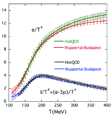
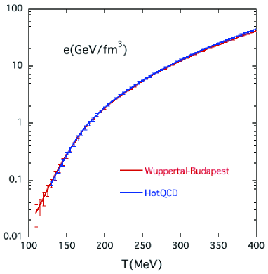
Figure 15: Thermodynamic quantities in the continuum limit in 2+1 flavor QCD as a function of temperature. Left panel shows the energy density $e/T^{4}$ and interaction measure $I/T^{4}=(e-3p)/T^{4}$ in units of $T^{4}$, and right panel shows energy density $e$ in units of GeV/fm³. From Refs. WBEoS2014 ; HotQCD2014 . Color online.

In the left panel of Fig. 15 we show the energy density $e/T^{4}$ and interaction measure $I/T^{4}=(e-3p)/T^{4}$, with $p$ the pressure, in units of $T^{4}$ calculated in the staggered quark formalism by two groups WBEoS2014 ; HotQCD2014 . They are obtained at the physical quark masses, and infinite volume and continuum extrapolations are made. We observe very good agreement up to about 200 MeV beyond which a one standard deviation difference appears. Physically important is the feature that the Stefan-Boltzmann value for free gluons and quarks, $e_{\rm SB}/T^{4}=\pi^{2}(8+21N_{f}/4)/15=15.62\cdots$ for $N_{f}=3$, is reached only slowly, with significant deviations remaining at $T/T_{c}\sim 2-3$. This indicates that the quark-gluon matter is strongly interacting at these temperature ranges. The right panel shows the energy density in units of GeV/fm³.

Experimental effort toward detection of quark-gluon plasma through heavy ion collisions in accelerators has been going on for a long time. It started with the Bevalac at Berkeley in the 70’s, the AGS at BNL and the SPS at CERN in the 80’s, with RHIC at BNL since 2000 and with the LHC at CERN most recently.

Let us see how lattice QCD predictions compare with heavy ion experiments at RHIC and the LHC. Phenomenological estimates on the energy density reached at the initial stage of the collision range from $e\approx 5.6$ GeV/fm³ for Au–Au collisions at RHIC with $\sqrt{s_{NN}}=200$ GeV PHENIX2005 , to $e\approx 15$ GeV/fm³ for Pb–Pb collisions at the LHC with $\sqrt{s_{NN}}=2.76$ TeV CMS2012 . Looking at the right panel of Fig. 15 we read out a temperature of order $T\approx 200$ MeV and $300$ MeV, respectively, for these energy densities which are high enough for the collision product to be in the high temperature phase. For comparison, an experimental estimate of the temperature using the low $p_{T}$ excess of direct photons that are supposed to come from the initial thermalized state gave $T=221(27)$ MeV at RHIC PHENIX2010 and $T=304(51)$ MeV at the LHC ALICE2012 .

The initial fireball rapidly cools as it expands, and hadrons are formed once the temperature falls below the transition temperature $T_{c}$. It has been known that the yield of various hadrons from the collision could be well fitted with statistical thermal distribution parametrized by a chemical freeze out temperature $T_{f}$. This temperature increases with the collision energy and saturates at $T_{f}\approx 160$ MeV at RHIC energies Andronic2009 , though slightly decreasing at LHC energies.

Furthermore, the azimuthal anisotropy in the transverse hadron yields, quantified in terms of the elliptic flow $v_{2}$ and higher moments where $v_{n}=\langle\cos n\phi\rangle$, is well described by hydrodynamical models with no or small viscosity and using the equation of state from lattice QCD.

Thus, while small viscosity was a surprise, the experimental data are broadly consistent with the production of strongly interacting high temperature quark-gluon matter with the properties as predicted by lattice QCD. It is interesting to note that small shear viscosity close to the quantum limit $\eta/s=1/4\pi$ Kovtunetal2005 is observed by lattice QCD calculations of transport coefficients in the pure gluon case NakamuraSakai2006 ; Meyer2007 .

From a heavy-ion collision point of view, the transition temperature and equation of state are only indirectly reflected in the characteristics of the final hadronic state. The moments of conserved charges such as electric charge $Q$, strangeness $S$, and baryon number $B$ provide interesting quantities which are calculable in lattice QCD and are directly observable in experiments. Thus they have been attracting much interest recently Stephanovetal1999 ; EjiriKarschRedlich2006 ; Karsch2012 ; Bazabovetal2012 ; Borsanyietal2014 .

4.4.4 Dynamics at finite baryon number density

Theoretical expectations on the phases of QCD at finite temperature $T$ and finite baryon number density $\rho_{B}$ is depicted in Fig. 16. The chiral crossover transition at $T_{c}\approx 150-160$ MeV continues into the finite $\rho_{B}$ region, and hits a second order critical point at some $(T_{E},\rho_{E})$ beyond which the transition turns into a first order phase transition. For sufficiently large baryon number density, one expects novel phases such as a color superconductor.

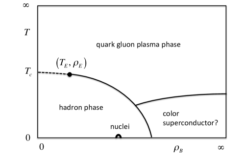
Figure 16: Schematic phase diagram of QCD on the temperature baryon density plane..

Finite baryon number density can be introduced by adding a quark chemical potential $\mu$ to the Hamiltonian. On a lattice, this is achieved by multiplying the positive temporal hopping term of the quark action by $\exp(\mu a)$, and the negative hopping term by $\exp(-\mu a)$.

Solid quantitative results are still not available on the phase diagram. The main reason is that for non-zero quark chemical potential, the quark Dirac determinant $\det D(U,\mu)$ is complex, so that the Monte Carlo methods based on a probability interpretation of the weight $\det D\cdot\exp(-S_{G}(U))$ no longer work in general.

One can see the difficulty by defining the phase of the determinant by

$$\theta(U,\mu)=-i\log\frac{\det D(U,\mu)}{|\det D(U,.\mu)|},$$ (81)

and rewriting expectation values in the following way:

$$\left<O\right> = \frac{\left<O\exp\left(i\theta(U,\mu)\right)\right>_{||}}{\left<\exp\left(i\theta(U,\mu)\right)\right>_{||}},$$ (82)

where $\left<\cdot\right>_{||}$ means the average with respect to the phase quenched determinant $|\det D(U,\mu)|$. The quenched average of the phase factor in the denominator is a ratio of the two partition functions:

$$\left<\exp\left(i\theta(U,\mu)\right)\right>_{||} = \frac{Z(\mu)}{Z_{||}(\mu)},$$ (83)

$$Z_{||}(\mu) = \int\prod_{n\mu}dU_{n\mu}|\det D(U,\mu)|\exp(S_{\rm gluon}(U)).$$ (84)

If the quenched average defines a statistical system with a free energy density $f_{||}(\mu)$, one can write

$$\left<\exp\left(i\theta(U,\mu)\right)\right>_{||}=\exp\left(-\frac{V(f(\mu)-f_{||}(\mu)}{T}\right),$$ (85)

with $f(\mu)$ the free energy density of the original system. The right hand side vanishes exponentially fast for large spatial volumes $V\to\infty$. This is one way of explaining the sign problem.

A variety of methods have been devised and explored to overcome this problem. Besides the phase quenched calculation described above, they include reweighting of the determinant FodorKatz2001 , analytic continuation from imaginary chemical potential RobergeWeiss1986 ; ForcrandPhilipsen2002 , Taylor expansion in powers of $\mu/T$ Alltonetal2003 ; Ejirietal2012 , canonical ensemble simulation Lietal , complex Langevin simulation Aartsetal ; Sexty2013 , and others. These methods have yielded some success for not too large values of $\mu/T$. The main problem, however, has been the difficulty of controlling errors in the results. The precise location of the critical point E and physics of finite density QCD for larger baryon number density is still largely open at present.

5 Conclusions

Lattice QCD is a major contribution of Kenneth Wilson to physics. In our view, it is on a par in significance with his renormalization group theory of critical phenomena which won him Nobel Prize in Physics in 1982. Conceptually, it clarified how quantum fluctuations of gauge fields give rise to a confining force which is essentially distinct in its origin from the forces arising from exchange of a particle such as the electromagnetic force. At the same time, coupled with supercomputers, it opened a way to calculate the physical predictions from its first principles, making possible detailed comparisons with experiment.

In 2004, Kenneth Wilson delivered a talk entitled “The Origins of Lattice Gauge Theory” at International Symposium on Lattice Field Theory held at Fermi National Accelerator Laboratory Wilson2005 . Looking back on the development of lattice QCD, he said that “The lattice gauge theory was a discovery waiting to happen, once asymptotic freedom was established.”, and went on to describe works of his contemporaries who could have preceded or shared the discovery. Nonetheless it is clear that, because of his previous studies leading to his encounter with statistical mechanics and phase transitions, he was in a unique position to be the first to grasp the deep significance of strongly coupled gauge dynamics in relation to confinement.

In the same article, he commended on the vast progress in lattice QCD in the thirty years since 1974, the year of his seminal paper Wilson1974 , due “in part to improved algorithms, in part to increased computing power, and in part to the increased scale of the research effort underway today”, but urged on that “this does not mean that the present state of lattice gauge computations is fully satisfactory. The knowledge and further advances that will likely accumulate over the next thirty years should be just as profound”.

As if corroborating his view, in just a decade since then, the physical point computation was realized, and many beautiful physics results ensued, as summarized in Sec. 4.

The past decade, then, was a turning point of lattice QCD in our view; prior to this event, despite the premise that it provided a first-principle calculation, it remained a method of uncertain reliability, requiring chiral extrapolations which were difficult to control. We are now able to calculate and understand many properties of hadron states including masses and matrix elements, at the physical quark masses and controlling errors of calculations. The precision of the calculation has now reached the level of a few % or better in many quantities. Consequently, important constraints are now available on the CKM matrix elements and CP violation in the Standard Model.

This is not to say that progress has been uniform in all fronts. In thermodynamics of QCD, while some basic quantities such as the transition temperature and equation of state have been calculated, the region of finite baryon number density is still largely unexplored. A major methodological breakthrough will be needed to extend our understanding to the entire phase diagram of QCD.

One area which did not even exist at the time of Wilson’s talk in 2004 is nuclear physics based on lattice QCD. In fact, while there were pioneering studies on H di-baryon in the late 80’s Mackenzie1985 ; Iwasaki1988 and nucleon scattering lengths in 1994 Fukugitaetal1994 , it is in 2007 that the two nucleon potential was first extracted from lattice QCD Ishiietal2007 , and in 2009 that the binding energy of Helium was calculated directly from Helium correlation function  Yamazakietal2009 . This is a challenging area in terms of physics as well as in calculational techniques; one has to deal with a small energy scale of 0(10) MeV, the number of Wick contractions for quark fields increases factorially fast with the mass number, and so does the statistical error of nuclei propagators for large time separations.

In theoretical physics, theory and computing go hand in hand. Calculations are indispensable in order to confirm the validity of theory, and even more so to explore the consequences of theory which help us better understand why our world works the way it does. Lattice QCD is a prime example of such a relationship between theory and computing. Kenneth Wilson clearly foresaw the importance and future potential of supercomputing in this connection, and many of his thoughts and vision in the early 80’s Lax1982 came to be realized since then. Looking toward future, as he prophesied Wilson1983 , our understanding of the strong interactions will become more profound as the computing power increases toward exascale and possibly beyond in the decades to come.

References

- (1) K. G. Wilson, Confinement of Quarks, Cornell preprint CLNS-262 (Feb 1974), published in Phys. Rev. D10 (1974) 2445.
- (2) K. G. Wilson, Future Directions in Particle Theory, in Proceedings of the 1983 Lepton Photon Symposium at High Energies, p.812 (Cornell University Press, 1983).
- (3) K. G. Wilson, The Origins of Lattice Gauge Theory, Nucl. Phys. B (Proc. Suppl.) 140 (2005) 3.
- (4) M. Creutz, L. Jacobs, C. Rebbi, Experiments with a Gauge Invariant Ising System, Phys. Rev. Lett. 42 (1979) 1390.
- (5) K. G. Wilson, Monte Carlo Calculations for the Lattice Gauge Theory, in Proceedings of the 1979 Cargese Summer Institute, NATO Sci. Ser. B59 (1980) 363.
- (6) M. Creutz, Solving Quantized SU(2) Gauge Theory, Brookhaven National Laboratory Print-79-0919 (Sep 1979); Monte Carlo Study of Quantized SU(2) Gauge Theory, Phys. Rev. D21 (1980) 2308.
- (7) D. Weingarten, Monte Carlo Evaluation of Hadron Masses in Lattice Gauge Theories with Fermions, Phys. Lett. B109 (1982) 57.
- (8) H. Hamber and G. Parisi, Numerical Estimates of Hadronic Masses in a Pure SU(3) Gauge Theory, Phys. Rev. Lett. 47 (1981) 1792.
- (9) Particle Data Group web page http://pdg.lbl.gov
- (10) D. J. Gross and F. Wilczek, Ultraviolet Behavior of non-Abelian Gauge Theories, Phys. Rev. Lett. 30 (1974) 1343.
- (11) H. D. Politzer, Reliable Perturbative Results for Strong Interactions?, Phys. Rev. Lett. 30 (1974) 1346.
- (12) K. Symanzik, Euclidean quantum field theory, in Local quantum field theory, p. 152, edited by R. Jost (New York: Academic Press 1969).
- (13) K. G. Wilson and J. Kogut, The Renormalization Group and the Expansion, Phys. Rep. 12 (1974) 75.
- (14) K. Osterwalder, R. Schrader, Axioms for Euclidean Green’s Functions, Commun. Math. Phys. 31 (1973) 83; Axioms for Euclidean Green’s Functions II, Commun. Math. Phys. 42 (1975) 281.
- (15) G. S. Bali, K. Schilling, Running Coupling and the Lambda Parameter from SU(3) Lattice Simulations, Phys. Rev. D47 (1993) 661.
- (16) K. C. Bowler, A. Hasenfratz, P. Hasenfratz, U. M. Heller, F. Karsch, R. D. Kenway, G. S. Pawley, D. J. Wallace, The SU(3) Beta Function at Large Beta, Phys. Lett. B179 (1986) 375.
- (17) R. Gupta, G. W. Kilcup, A. Patel , S. R. Sharpe, The Beta Function for Pure Gauge SU(3), Phys. Lett. B211 (1988) 132.
- (18) M. Lüscher, R. Sommer, P. Weisz. U. Wolff, A Precise Determination of the Running Coupling in the SU(3) Yang-Mills Theory, Nucl. Phys. B413 (1994) 481.
- (19) ALPHA Collaboration, M. Della Morte, R. Frezzotti, J. Heitger, J. Rolf, R. Sommer, U. Wolff, Computation of the Strong Coupling in QCD with Two Dynamical Flavours, Nucl. Phys. B713 (2005) 378.
- (20) PACS-CS Collaboration, S. Aoki, K. I. Ishikawa, N. Ishizuka, T. Izubuchi, D. Kadoh, K. Kanaya, Y. Kuramashi, K. Murano, Y. Namekawa, M. Okawa, Y. Taniguchi, A. Ukawa, N. Ukita, T. Yoshié, Precise Determination of the Strong Coupling Constant in Lattice QCD with the Schrödinger Functional Scheme, JHEP 0910 (2009) 053.
- (21) R. Sommer, F. Tekin, U. Wolff, Running of the SF-coupling with Four Massless Flavours, PoS(Lattice 2010) (2010) 241.
- (22) L. H. Karsten, J. Smit, Lattice Fermions, Species Dubling, Chiral Invariance and the Triangle Anomaly, Nucl. Phys. B183 (1981) 103.
- (23) H. B. Nielesen and M. Ninomiya, Absence of Neutrinos on a Lattice. 1. Proof by Homotopy Theory, Nucl. Phys. B185 (1981) 20; Erratum-ibid. B195 (1982) 541.
- (24) L. H. Karsten, Lattice Fermions in Euclidean Space-time, Phys. Lett. B104 (1981) 315.
- (25) K. G. Wilson, Quarks and strings on a lattice, in New Phenomena in Subnuclear Physics, Proceedings of the 14th Course of the International School of Subnuclear Physics, Erice, 1975, edited by A. Zichichi (Plenum, New York, 1977).
- (26) M. Bochicchio, L. Maiani, G. Martinelli, G. C. Rossi, M. Testal, Chiral Symmetry on the Lattice with Wilson Fermions, Nucl. Phys. B262 (1985) 331.
- (27) S. Itoh, Y. Iwasaki, Y. Oyanagi, T. Yoshié, Hadron Spectrum in Quenched QCD on a Lattice With Renormalization Group Improved Lattice SU(3) Gauge Action, Nucl. Phys. B274 (1986) 33.
- (28) N. Kawamoto, Towards the Phase Structure of Euclidean Lattice Gauge Theories with Fermions, Nucl. Phys. B190 (1981) 617.
- (29) S. Aoki, New Phase Structure for Lattice QCD with Wilson Fermions, Phys. Rev. D30 (1984) 2653.
- (30) R. Frezzotti, P. Grassi, S. Sint, P. Weisz, Lattice QCD with a Chirally Twisted Mass Term, JHEP 0108 (2001) 058.
- (31) R. Frezzotti, G. C. Rossi, Chirally improving Wilson Fermions - I. O(a) Improvement, JHEP 08 (2004) 007.
- (32) S. Aoki, O. Baer, Automatic Improvement for Twisted Mass QCD in the Presence of Spontaneous Symmetry Breaking, Phys. Rev. D74 (2006) 034511.
- (33) L. Susskind, Lattice Fermions, Phys. Rev. D16 (1977) 3031.
- (34) H. S. Sharatchandra, H. J. Thus, P. Weisz, Susskind Fermions on a Euclidean lattice, Nucl. Phys. B192 (1981) 205.
- (35) H. Kluberg-Stern, A. Morel, O. Napoly, B. Petersson, Flavors of Lagrangian Susskind Fermions, Nucl. Phys. B220 (1983) 447.
- (36) S. R. Sharpe, Rooted Staggered Fermions: Good, Bad or Ugly?, PoS (Lattice 2006) (2006) 022.
- (37) W.-J. Lee, S. R. Sharpe, Partial Flavor Symmetry Restoration for Chiral Staggered Fermions, Phys. Rev. D60 (1999) 114503.
- (38) P. H. Ginsparg and K. G. Wilson, A Remnant of Chiral Symmetry on the Lattice, Phys. Rev. D25 (1982) 2649.
- (39) M. Lüscher, Exact Chiral Symmetry on the Lattice and the Ginsparg-Wilson Relation, Phys. Lett. B428 (1998) 342.
- (40) D. B. Kaplan, A Method for Simulating Chiral Fermions on the Lattice, Phys. Lett. B288 (1992) 342.
- (41) V. Furman, Y. Shamir, Axial Symmetries in Lattice QCD with Kaplan Fermions, Nucl. Phys. B439 (1995) 54.
- (42) R. Narayanan and H. Neuberger A Construction of Lattice Chiral Gauge Theories, Nucl. Phys. B443 (1995) 305.
- (43) H. Neuberger, Exactly Massless Quarks on the Lattice, Phys. Lett. B417 (1998) 141.
- (44) H. Neuberger, Vector-like Gauge Theories with Almost Massless Fermions on the Lattice, Phys. Rev. D57 (1998) 5417.
- (45) A. Borici, Truncated Overlap Fermions, Nucl. Phys. B(Proc. Suppl.) 83 (2000) 771.
- (46) P. Hasenfratz, V. Laliena, F. Niedermayer, The Index Theorem in QCD with a Finite Cut-Off , Phys. Lett. B427 (1998) 125.
- (47) R. Arthur, T. Blum, P. A. Boyle, N. H. Christ, N. Garron, R. J. Hudspith, T. Izubuchi, C. Jung, C. Kelly, A. T. Lytle, R. D. Mawhinney, D. Murphy, S. Ohta , C. T. Sachrajda, A. Soni, J. Yu, and J. M. Zanotti (RBC and UKQCD Collaborations), Domain Wall QCD with Near-Physical Pions, Phys. Rev. D87 (2013) 094514.
- (48) S. Aoki, T.-W. Chiu, G. Cossu, X. Feng, H. Fukaya, S. Hashimoto, T.-H. Hsieh, T. Kaneko, H. Matsufuru, J. Noaki, Simulation of Quantum Chromodynamics on the Lattice with Exactly Chiral Lattice Fermions, PTEP 2012 (2012) 01A106.
- (49) A. Hasenfratz, P. Hasenfratz, F. Niedermayer, Simulating Full QCD with the Fixed Point Action, Phys. Rev. D72 (2005) 114508.
- (50) E. Eichten, Heavy Quarks on the Lattice, Nucl. Phys. Proc. Suppl. 4 (1988) 170.
- (51) G. P. Lepage and B. A. Thacker, Effective Lagrangians for Simulating Heavy Quark Systems, Nucl. Phys. Proc. Suppl. 4 (1988) 199.
- (52) A. X. El-Khadra, A. S. Kronfeld, P. B. Mackenzie Massive Fermions in Lattice Gauge Theory, Phys. Rev. D55 (1997) 3933.
- (53) S. Aoki, Y. Kuramashi, S. Tominaga, Relativistic Heavy Quarks on the Lattice, Prog. Theor. Phys. 109 (2003) 383.
- (54) N. H. Christ, M. Li, H.-W. Lin, Relativistic Heavy Quark Effective Action, Phys. Rev. D76 (2007) 074505.
- (55) N. Metropolis, A. W. Rosenbluth, M. N. Rosenbluth, A. H. Teller, and E. Teller, Equation of State Calculations by Fast Computing Machines, Journal of Chemical Physics 21 (1953) 1087.
- (56) K. G. Wilson, The Renormalization Group: Critical Phenomena and the Kondo Problem, Rev. Mod. Phys. 47 (1975) 773.
- (57) N. Andrei, J.H. Lowenstein, Scales and Scaling in the Kondo Model, Phys. Rev. Lett. 46 (1981) 356.
- (58) http://www.top500.org/lists/2014/11/
- (59) D. J. E. Callaway, A. Rahman, Microcanonical Ensemble Formulation of Lattice Gauge Theory, Phys. Rev. Lett. 49 (1982) 613.
- (60) J. Polonyi, H. W. Wyld, Microcanonical Simulation of Fermionic Systems, Phys. Rev. Lett. 51 (1983) 2257.
- (61) A. Ukawa. M. Fukugita, Langevin Simulation including Dynamical Quark Loops, Phys. Rev. Lett. 55 (1985) 1854.
- (62) G. G. Batrouni, G. R. Katz, A. S. Kronfeld, G. P. Lepage, B. Svetitsky, K. G. Wilson, Langevin Simulations of Lattice Field Theories, Phys. Rev. D32 (1985) 2736.
- (63) S. Duane, A. D. Kennedy, B. J. Pendleton, D. Roweth, Hybrid Monte Carlo, Phys. Lett. B195 (1987) 216.
- (64) A. Ukawa for CP-PACS and JLQCD Collaborations, Computational Cost of Full QCD Simulations experienced by CP-PACS and JLQCD Collaborations, Nucl. Phys. B(Proc. Suppl.) 106 (2002) 195.
- (65) M. Lüscher, Schwarz-preconditioned HMC Algorithm for Two-Flavour Lattice QCD, Comput. Phys. Commun. 165 (2005) 199.
- (66) J.C. Sexton and D.H. Weingarten, Hamiltonian Evolution for the Hybrid Monte Carlo Algorithm, Nucl. Phys. B380 (1992) 665.
- (67) S. Aoki, K.-I. Ishikawa, N. Ishizuka, T. Izubuchi, D. Kadoh, K. Kanaya, Y. Kuramashi, Y. Namekawa, M. Okawa, Y. Taniguchi, A. Ukawa, N. Ukita, and T. Yoshié (PACS-CS Collaboration), 2+1 Flavor Lattice QCD toward the Physical Point, Phys. Rev. D79 (2009) 034503.
- (68) M.Hasenbusch, Speeding up the Hybrid Monte Carlo Algorithm for Dynamical Fermions, Phys. Lett. B519 (2001) 177.
- (69) I. Horvath, A. D. Kennedy, S. Sint, A New Exact Method for Dynamical Fermion Computations with Non-local Actions , Nucl. Phys. B(Proc. Suppl.) 73 (1999) 834.
- (70) M. Lüscher, Local Coherence and Deflation of the Low Quark Modes in Lattice QCD, JHEP 0707 (2007) 081.
- (71) R. Babich, J. Brannick, R. C. Brower, M. A. Clark, T.A. Manteuffel, S. F. McCormick, J. C. Osborn, C. Rebbi, Adaptive Multigrid Algorithm for the Lattice Wilson-Dirac Operator, Phys. Rev. Lett. 105 (2010) 201602.
- (72) A. Frommer, K. Kahl, S. Krieg, B. Leder, M. Rottmann, Adaptive Aggregation Based Domain Decomposition Multigrid for the Lattice Wilson Dirac Operator, e-Print: arXiv:1303.1377 [hep-lat]
- (73) F. Butler, H. Chen, J. Sexton, A. Vaccarino, D. Weingarten, Hadron Mass Predictions of the Valence Approximation to Lattice QCD, Phys. Rev. Lett. 70 (1993) 2849.
- (74) CP-PACS Collaboration: S. Aoki, G. Boyd, R. Burkhalter, S. Ejiri, M. Fukugita, S. Hashimoto, Y. Iwasaki, K. Kanaya, T. Kaneko, Y. Kuramashi, K. Nagai, M. Okawa, H. P. Shanahan, A. Ukawa, T. Yoshié, Quenched Light Hadron Spectrum, Phys. Rev. Lett. 84 (2000) 238.
- (75) CP-PACS Collaboration: A. Ali Khan, S. Aoki, G. Boyd, R. Burkhalter, S. Ejiri, M. Fukugita, S. Hashimoto, N. Ishizuka, Y. Iwasaki, K. Kanaya, T. Kaneko, Y. Kuramashi, T. Manke, K. Nagai, M. Okawa, H.P. Shanahan, A. Ukawa, T. Yoshié, Dynamical Quark Effects on Light Quark Masses, Phys. Rev. Lett. 85 (2000) 4674; Erratum-ibid. 90 (2003) 029902.
- (76) S. Durr, Z. Fodor, J. Frison, C. Hoelbling, R. Hoffmann, S. D. Katz, S. Krieg, T. Kurth, L. Lellouch, T. Lippert, K. K. Szabo, G. Vulvert, Ab-Initio Determination of Light Hadron Masses, Science 322 (2008) 1224.
- (77) Martin Lüscher, Two Particle States on a Torus and their Relation to the Scattering Matrix, Nucl. Phys. B354 (1991) 531; Signatures of Unstable Particles in Finite Volume, Nucl. Phys. B364 (1991) 237.
- (78) A. Duncan, E. Eichten, H. Thacker, Electromagnetic Splittings and Light Quark Masses in Lattice QCD, Phys. Rev. Lett. 76 (1996) 3894.
- (79) T. Blum, R. Zhou, T. Doi, M. Hayakawa, T. Izubuchi, S. Uno, N. Yamada, Electromagnetic Mass Splittings of the Low Lying Hadrons and Quark Masses from 2+1 Flavor Lattice QCD+QED, Phys. Rev. D82 (2010) 094508.
- (80) T. Ishikawa, T. Blum, M. Hayakawa, T. Izubuchi, C. Jung, R. Zhou, Full QED+QCD Low-Energy Constants through Reweighting, Phys. Rev. Lett. 109 (2012) 072002.
- (81) S. Aoki, K.-I. Ishikawa, N. Ishizuka, K. Kanaya, Y. Kuramashi, Y. Nakamura, Y. Namekawa, M. Okawa, Y. Taniguchi, A. Ukawa, N. Ukita, T. Yoshié (PACS-CS Collaboration), 1+1+1 flavor QCD + QED Simulation at the Physical Point, Phys. Rev. D86 (2012) 034507.
- (82) S. Borsanyi, S. Durr, Z. Fodor, C. Hoelbling, S. D. Katz, S. Krieg, L. Lellouch, T. Lippert, A. Portelli, K. K. Szabo, Ab initio Calculation of the Neutron-Proton Mass Difference, arXiv:1406.4088 (2014).
- (83) S. Aoki, M. Fukugita, K-I. Ishikawa, N. Ishizuka, K. Kanaya, Y. Kuramashi, Y. Namekawa, M. Okawa, K. Sasaki, A. Ukawa, and T. Yoshié, Lattice QCD Calculation of the Meson Decay Width, Phys. Rev. D 76 (2007) 094506; Meson Decay in Flavor Lattice QCD, Phys. Rev. D84 (2011) 094505.
- (84) A. Bazavov, C. Bernard, C. DeTar, X. Du, W. Freeman, S. Gottlieb, U. M. Heller, J. E. Hetrick, J. Laiho, L. Levkova, M. B. Oktay, J. Osborn, R. Sugar, D. Toussaint, R. S. Van de Water (The MILC Collaboration), MILC Results for Light Pseudo Scalars, PoS (CD09) (2009) 007.
- (85) S. Durr, Z. Fodor, C. Hoelbling, S. Katz, S. Krieg et al., Lattice QCD at the Physical Point: Light Quark Masses, Phys. Lett. B701 (2011) 265.
- (86) Particle Data Group Collaboration (C. Caso et al.), Review of Particle Physics, Eur. Phys. J. C3 (1998) 1.
- (87) Particle Data Group Collaboration (J. Beringer et al.), Review of Particle Physics, Phys. Rev. D86 (2012) 010001.
- (88) ”Quantum Chromodyamics” section in http://pdg.lbl.gov/2013/reviews/.
- (89) C. McNeile, C. T. H. Davies, E. Follana, K. Hornbostel, G. P. Lepage, High-Precision c and b Masses and QCD Coupling from Current-Current Correlators in Lattice and Continuum QCD, Phys. Rev. D82 (2010) 034512.
- (90) A. Bazavov, N. Brambilla, X. Garcia i Tormo, P. Petreczky, J. Soto, A. Vairo, Determination of from the QCD Static Energy, Phys. Rev. D86 (2012) 114031.
- (91) http://www.utfit.org/UTfit/
- (92) http://http://ckmfitter.in2p3.fr
- (93) http://www.slac.stanford.edu/xorg/hfag/
- (94) FLAG Working Group, S. Aoki, Y. Aoki, C. Bernard, T. Blum, G. Colangelo, M. Della Morte, S. Durr, A. X. El-Khadra, H. Fukaya, R. Horsley, A. Juttner, T. Kaneko, J. Laiho, L. Lellouch, H. Leutwyler, V. Lubicz, E. Lunghi, S. Necco, T. Onogi, C. Pena, C. T. Sachrajda, S. R. Sharpe, S. Simula, R. Sommer, R. S. Van de Water, A. Vladikas, U. Wenger, H. Wittig, Review of Lattice Results concerning Low Energy Particle Physics, ArXive:1310.8555 ( August 2014).
- (95) A. Bazavov, C. Bernard, C. M. Bouchard, C. DeTar, M. Di Pierro, A. X. El-Khadra, R. T. Evans, E. D. Freeland, E. Gamiz, S. Gottlieb, U. M. Heller, J. E. Hetrick, R. Jain, A. S. Kronfeld, J. Laiho, L. Levkova, P. B. Mackenzie, E. T. Neil, M. B. Oktay, J. N. Simone, R. Sugar, D. Toussaint, R. S. Van de Water, Neutral B-meson Mixing from Three-Flavor Lattice QCD: Determination of the SU(3)-Breaking Ratio , Phys. Rev. D86 (2012) 034503.
- (96) E. Gulez, A. Gray, M. Wingate, C. T. H. Davies, G. P. Lepage, J. Shigemitsu, B Meson Semileptonic Form Factors from Unquenched Lattice QCD, Phys. Rev. D73 (2006) 074502.
- (97) J. A. Bailey, C. Bernard, C. DeTar, M. Di Pierro, A. X. El-Khadra, R. T. Evans, E. D. Freeland, E. Gamiz, S. Gottlieb, U. M. Heller, J. E. Hetrick, A. S. Kronfeld, J. Laiho, L. Levkova, P. B. Mackenzie, M. Okamoto, J. N. Simone, R. Sugar, D. Toussaint, R. S. Van de Water, The Semi-Leptonic Form Factor from Three-Flavor Lattice QCD: A Model-Independent Determination of , Phys. Rev. D79 (2009) 054507.
- (98) J. A. Bailey, A. Bazavov, C. Bernard, C. M. Bouchard, C. DeTar, D. Du, A. X. El-Khadra, J. Foley, E. D. Freeland, E. Gámiz, S. Gottlieb, U. M. Heller, A. S. Kronfeld, J. Laiho, L. Levkova, P. B. Mackenzie, E. T. Neil, S.-W. Qiu, J. Simone, R. Sugar, D. Toussaint, R. S. Van de Water, R. Zhou, Update of from the Form Factor at Zero Recoil with Three-Flavor Lattice QCD, Phys. Rev. D89 (2014) 114504.
- (99) V. Fanti et al, A New Measurement of Direct CP Violation in Two Pion Decays of the Neutral Kaon, Phys. Lett. B465 (1999) 335.
- (100) A. Arabi-Harati et al, Measurements of Direct CP Violation, CPT Symmetry, and Other Parameters in the Neutral Kaon System, Phys. Rev. D67 (2003) 012005.
- (101) G. Buchalla, A. J. Buras, M. K. Harlander, The Anatomy of in the Standard Model , Nucl. Phys. B337 (1990) 313; G. Buchalla, A. J. Buras, M. E. Lautenbacher, Weak Decays beyond Leading Logarithms, Rev. Mod. Phys. 68 (1996) 1125.
- (102) A. Donini, V. Gimenez, G. Martinelli, M. Talevi, A. Vladikas, Non-Perturbative Renormalization of Lattice Four-Fermion Operators without Power Subtractions, Eur. Phys. J. C10 (1999) 121.
- (103) N. Ishizuka, K. I. Ishikawa, A. Ukawa, T. Yoshié, Calculation of Decay Amplitudes with Improved Wilson Fermion, arXiv:1311.0958(2013).
- (104) L. Lellouch, M. Lüscher, Weak Transition Matrix Elements from Finite Volume Correlation Functions, Commun. Math. Phys. 219 (2001) 31.
- (105) T. Blum, P. A. Boyle, N. H. Christ, N. Garron, E. Goode, T. Izubuchi, C. Jung, C. Kelly, C. Lehner, M. Lightman, The Decay Amplitude from Lattice QCD, Phys. Rev. Lett. 108 (2012) 141601; Phys. Rev. D86 (2012) 074513.
- (106) F. R. Brown, F. P. Butler, H. Chen, N. H. Christ, Z.-H. Dong, W. Schaffer, L. I. Unger, A. Vaccarino, On the Existence of a Phase Transition for QCD with Three Light Quarks, Phys. Rev. Lett. 65 (1990) 2491.
- (107) K. Kanaya, Finite Temperature QCD on the Lattice – Status 2010, PoS (Lattice 2010) (2010) 012.
- (108) A. M. Polyakov, Thermal Properties of Gauge Fields and Quark Liberation, Phys. Lett. 72B (1978) 477.
- (109) L. Susskind, Hot Quark Soup, Phys. Rev. D20 (1979) 2610.
- (110) L. G. Yaffe, B. Svetitsky, First Order Phase Transition in the SU(3) Gauge Theory at Finite Temperature, Phys. Rev. D26 (1982) 963.
- (111) T. Banks, A. Ukawa, Deconfining and Chiral Phase Transitions in Quantum Chromodynamics at Finite Temperature, Nucl. Phys. B225 (1983) 145.
- (112) R. D. Pisarski, F. Wilczek, Remarks on the Chiral Phase Transition in Chromodynamics, Phys. Rev. D29 (1984) 338.
- (113) S. Gavin, A. Gocksch, R. D. Pisarski, QCD and the Chiral Critical Point , Phys. Rev. D49 (1994) 3079.
- (114) K. Rajagopal, The Chiral Phase Transition in QCD: Critical Phenomena and Long Wavelength Pion Oscillations, Quark-gluon plasma vol.2 (1995) (arXiv: hep-ph/9504310).
- (115) For example, see, M. N. Barber, Finite Size Scaling, Phase Transitions and Critical Phenomena Vol. 8 (1973), edited by C. Domb and J. Lewobitz (Academic Press).
- (116) M. Fukugita, M. Okawa, A. Ukawa, Order of the Deconfining Phase Transition in SU(3) Lattice Gauge Theory, Phys. Rev. Lett. 63 (1989) 1768; Finite Size Scaling Study of the Deconfining Phase Transition in Pure SU(3) Lattice Gauge Theory, Nucl. Phys. B337 (1990) 181.
- (117) JLQCD Collaboration: S. Aoki, M. Fukugita, S. Hashimoto, K-I. Ishikawa, N. Ishizuka, Y. Iwasaki, K. Kanaya, T. Kaneda, S. Kaya , Y. Kuramashi, M. Okawa, T. Onogi, S. Tominaga, N. Tsutsui, A. Ukawa, N. Yamada, T. Yoshié, Phase Structure of Lattice QCD at Finite Temperature for 2+1 Flavors of Kogut-Susskind Quarks, Nucl. Phys. B (Proc.Suppl.) 73 (1999) 459.
- (118) F. Karsch, E. Laermann, C. Schmidt, The Chiral Critical Point in Three-Flavor QCD, Phys. Lett. B520 (2001) 41.
- (119) H.-T. Ding, A. Bazavov, P. Hegde, F. Karsch, S. Mukherjee, P. Petreczky, Exploring Phase Diagram of QCD at with HISQ Fermions, PoS (Lattice 2011) (2011) 191.
- (120) S. Aoki, M. Fukugita, S. Hashimoto, N. Ishizuka, Y. Iwasaki, K. Kanaya, Y. Kuramashi, H. Mino, M. Okawa, A. Ukawa, and T. Yoshié (JLQCD Collaboration), Scaling Study of the Two Flavor Chiral Phase Transition with the Kogut-Susskind Quark Action in Lattice QCD, Phys. Rev. D57 (1998) 3910.
- (121) A. Ali Khan, S. Aoki, R. Burkhalter, S. Ejiri, M. Fukugita, S. Hashimoto, N. Ishizuka, Y. Iwasaki, K. Kanaya, T. Kaneko, Y. Kuramashi, T. Manke, K. Nagai, M. Okamoto, M. Okawa, A. Ukawa, and T. Yoshié (CP-PACS Collaboration)), Phase Structure and Critical Temperature of Two Flavor QCD with Renormalization Group Improved Gauge Action and Clover improved Wilson Quark Action, Phys. Rev. D63 (2001) 034502.
- (122) C. Bonati, G. Cossu, M. D’Elia, A. Di Giacomo, C. Pica, The Order of the QCD Transition with Two Light Flavors, Nucl. Phys. A820 (2009) 243C.
- (123) S. Aoki, H. Fukaya, Y. Taniguchi, Chiral Symmetry Restoration, the Eigenvalue Density of the Dirac Operator, and the Axial U(1) Anomaly at Finite Temperature, Phys. Rev. D 86 (2012) 114512.
- (124) C. Bernard, T. Blum, C. DeTar, S. Gottlieb, U. M. Heller, J. E. Hetrick, K. Rummukainen, R. Sugar, D. Toussaint, M. Wingate, Which Chiral Symmetry is Restored in High Temperature Quantum Chromodynamics?, Phys. Rev. Lett. 78 (1997) 598.
- (125) S. Chandrasekharan, D. Chen, N. Christ, W. J. Lee, R. Mawhinney, P. Vranas, Anomalous Chiral Symmetry Breaking above the QCD Phase Transition, Phys. Rev. Lett. 82 (1999) 2463.
- (126) Y. Aoki, G. Endrodi, Z. Fodor, S. D. Katz, K. K. Szabo, The Order of the Quantum Chromodynamics Transition predicted by the Standard Model of Particle Physics, Nature 443 (2006) 675.
- (127) Y. Aoki, Z. Fodor, S.D. Katz, K.K. Szabo, The QCD Transition Temperature: Results with Physical Masses in the Continuum Limit, Phys. Lett. B643 (2006) 46; Wuppertal-Budapest Collaboration, S. Borsanyi, Z. Fodor, C. Hoelbling, S. D. Katz, S. Krieg, C. Ratti, K. K. Szabo, Is There still any Mystery in Lattice QCD? Results with Physical Masses in the Continuum Limit III, JHEP 1009 (2010) 073.
- (128) S. Borsanyi, Z. Fodor, C. Hoelbling, S. D. Katz, S. Krieg. K. K. Szabo, Full Result for the QCD Equation of State with 2+1 Flavors, Phys. Lett. B730 (2014) 99.
- (129) A. Bazavov, T. Bhattacharya, M. Cheng, C. DeTar, H.-T. Ding, S. Gottlieb, R. Gupta, P. Hegde, U. M. Heller, F. Karsch, E. Laermann, L. Levkova, S. Mukherjee, P. Petreczky, C. Schmidt, R. A. Soltz, W. Soeldner, R. Sugar, D. Toussaint, W. Unger, and P. Vranas (HotQCD Collaboration), Chiral and Deconfinement Aspects of the QCD Transition, Phys. Rev. D 85 (2012) 054503.
- (130) HotQCD Collaboration, A. Bazavov, T. Bhattacharya, C. DeTar, H.-T. Ding, S. Gottlieb, R. Gupta, P. Hegde, U. M. Heller, F. Karsch, E. Laermann, L. Levkova, S. Mukherjee, P. Petreczky, C. Schmidt, C. Schroeder, R. A. Soltz, W. Soeldner, R. Sugar, M. Wagner, P. Vranas, The Equation of State in 2+1-Flavor QCD, e-Print: arXiv:1407.6387 (2014)
- (131) PHENIX Collaboration, S. S. Adler et al., Systematic Studies of the Centrality and Dependence of the and in Heavy Ion Collisions at Mid-rapidity, Phys. Rev. C71 (2005) 034908.
- (132) CMS Collaboration, S. Chatrchyan et al., Measurement of the Pseudorapidity and Centrality Dependence of the Transverse Energy Density in Pb–Pb Collisions at TeV, Phys. Rev. Lett. 109 (2012) 152303.
- (133) PHENIX Collaboration, Enhanced Production of Direct Photons in Au+Au Collisions at GeV and Implications for the Initial Temperature, Phys. Rev. Lett. 104 (2010) 132301.
- (134) M. Wilde for ALICE Collaboration, Measurement of Direct Photons in pp and Pb-Pb Collisions with ALICE, arXiv.1210.5958 (2012)
- (135) A. Andronica, P. Braun-Munzinger, J. Stachel, Thermal Hadron Production in Relativistic Nuclear Collisions: The Hadron Mass Spectrum, the Horn, and the QCD Phase Transition, Phys. Lett. B673 (2009) 142.
- (136) P. Kovtun, D. T. Son, A. O. Starinets, Viscosity in Strongly Interacting Quantum Field Theories from Black Hole Physics, Phys. Rev. Lett. 94 (2005) 111601.
- (137) A. Nakamura, S. Sakai, Lattice Study of Gluon Viscosities: A Step towards RHIC Physics, Acta Phys. Polon. B37 (2006) 3371.
- (138) H. B. Meyer, A Calculation of the Shear Viscosity in SU(3) Gluodynamics, Phys. Rev. D76 (2007) 101701(R).
- (139) M. Stephanov, K. Rajagopal, E. Shyuriak, Event-by-Event Fluctuations in Heavy Ion Collisions and the QCD Critical Point, Phys. Rev. D60 (1999) 114028.
- (140) S. Ejiri, F. Karsch, K. Redlich, Hadronic Fluctuations at the QCD Phase Transition, Phys. Lett. B 633 (2006) 275.
- (141) F. Karsch, Determination of Freeze-out Conditions from Lattice QCD Calculations, Centr. Eur. J. phys. 10 (2102) 1234.
- (142) A. Bazavov, H.-T. Ding, P. Hegde, O. Kaczmarek, F. Karsch,E. Laermann, S. Mukherjee, P. Petreczky, C. Schmidt, D. Smith, W. Soeldner, M. Wagner, Freeze-Out Conditions in Heavy Ion Collisions from QCD Thermodynamics, Phys. Rev. Lett. 109 (2012) 192302.
- (143) S. Borsanyi, Z. Fodor, S. D. Katz, S. Krieg, C. Ratti, K. K. Szabo, Freeze-Out Parameters from Electric Charge and Baryon Number Fluctuations: Is There Consistency?, Phys. Rev. Lett. 113 (2014) 052301.
- (144) Z. Fodor, S. D. Katz, A New Method to Study Lattice QCD at Finite Temperature and Chemical Potential, Phys. Lett. B534 (2002) 87; Lattice Determination of the Critical Point of QCD at Finite T and , JHEP 0203 (2002) 014.
- (145) A. Roberge, N. Weiss, Gauge Theories with Imaginary Chemical Potential and the Phases of QCD, Nucl. Phys. B275 (1986) 734.
- (146) P. de Forcrand, O. Philipsen, The QCD Phase Diagram for Small Densities from Imaginary Chemical Potential, Nucl. Phys. B642 (2002) 290.
- (147) C. R. Allton, S. Ejiri, S. J. Hands, O. Kaczmarek, F. Karsch, E. Laermann, C. Schmidt, The Equation of State for Two Flavor QCD at Non-zero Chemical Potential, Phys. Rev. D68 (2003) 014507.
- (148) S. Ejiri, K. Kanaya, T. Umeda, Ab Initio Study of the Thermodynamics of Quantum Chromodynamics on the Lattice at Zero and Finite Densities, PTEP 2012 (2012) 01A104.
- (149) A. Li, A. Alexandru, K.-F. Liu, X. Meng, Finite Density Phase Transition of QCD with and using Canonical Ensemble Method, Phys. Rev. D82 (2010) 054502; A. Li, A. Alexandrou, K.-F. Liu, Critical Point of Nf=3 QCD from Lattice Simulations in the Canonical Ensemble, Phys. Rev. D84 (2011) 071503.
- (150) G. Aarts, I.-O. Stamatescu, Stochastic Quantization at Finite Chemical Potential, JHEP 0809 (2008) 018; G. Aarts, E. Seiler, I.-O. Stamatescu, The Complex Langevin Method: When can It be trusted?, Phys. Rev. D81 (2010) 054508.
- (151) D. Sexty, Simulating full QCD at Non-zero Density using the Complex Langevin Equation, Phys. Lett. B729 (2014) 108.
- (152) P. B. Mackenzie and H. B. Thacker, Evidence Against a Stable Dibaryon from Lattice QCD, Phys. Rev. Lett. 55 (1985) 2539.
- (153) Y. Iwasaki,T. Yoshié, Y. Tsuboi, The H Dibaryon in Lattice QCD, Phys. Rev. Lett. 60 (1988) 1371.
- (154) M. Fukugita, Y. Kuramashi, H. Mino, M. Okawa, A. Ukawa, An Exploratory Study of Nucleon-Nucleon Scattering Lengths in Lattice QCD, Phys. Rev. Lett. 73 (1994) 2176; M. Fukugita, Y. Kuramashi, M. Okawa, H. Mino, A. Ukawa, Hadron Scattering Lengths in Lattice QCD, Phys. Rev. D52 (1995) 3003.
- (155) N. Ishii, S. Aoki, T. Hatsuda, The Nuclear Force from Lattice QCD, Phys. Rev. Lett. 99 (2007) 022001.
- (156) T. Yamazaki, Y. Kuramashi, and A. Ukawa (PACS-CS Collaboration), Helium Nuclei in Quenched Lattice QCD, Phys. Rev. D81 (2010) 111504.
- (157) P. D. Lax, chairman, report of the panel on Large Scale Computing in Science and Engineering, 1982 (scanned pdf file is found at http://www.pnl.gov/scales/docs/lax_report1982.pdf).