A note on boundary kernels for distribution function estimation

Abstract

The use of second order boundary kernels for distribution function estimation was recently addressed in the literature (C. Tenreiro, 2013, Boundary kernels for distribution function estimation, REVSTAT–Statistical Journal, 11, 169–190). In this note we return to the subject by considering an enlarged class of boundary kernels that shows it self to be especially performing when the classical kernel distribution function estimator suffers from severe boundary problems.

Keywords: Distribution function estimation; kernel estimator; boundary kernels.

AMS 2010 subject classifications: 62G05, 62G20

1 Introduction

Given $X_{1},\dots,X_{n}$ independent copies of an absolutely continuous real random variable with unknown density and distribution functions $f$ and $F$, respectively, the classical kernel estimator of $F$ introduced by authors such as Tiago de Oliveira (1963), Nadaraya (1964) or Watson and Leadbetter (1964), is defined, for $x\in\mathbb{R}$, by

$$\bar{F}_{nh}(x)=\frac{1}{n}\sum_{i=1}^{n}\bar{K}\left(\frac{x-X_{i}}{h}\right),$$ (1)

where, for $u\in\mathbb{R}$,

$$\bar{K}(u)=\int_{-\infty}^{u}K(v)dv,$$

with $K$ a kernel on $\mathbb{R}$, that is, a bounded and symmetric probability density function with support $[-1,1]$ and $h=h_{n}$ a sequence of strictly positive real numbers converging to zero when $n$ goes to infinity. For some recent references on this classical estimator see Giné and Nickl (2009), Chacón and Rodríguez-Casal (2010), Mason and Swanepoel (2011) and Chacón, Monfort and Tenreiro (2014).

If the support of $f$ is known to be the finite interval $[a,b]$, the previous kernel estimator suffers from boundary problems if $F_{+}^{\prime}(a)\neq 0$ or $F_{-}^{\prime}(b)\neq 0$. This question is addressed in Tenreiro (2013) by extending to the distribution function estimation framework the approach followed in nonparametric regression and density function estimation by authors such as Gasser and Müller (1979), Rice (1984), Gasser et al. (1985) and Müller (1991). Specially, the author considers the boundary modified kernel distribution function estimator given by

$$\tilde{F}_{nh}(x)=\left\{\begin{array}[]{ll}0,&x\leq a\\ {\displaystyle\frac{1}{n}\sum_{i=1}^{n}\bar{K}_{x,h}\left(\frac{x-X_{i}}{h}\right)},&a<x<b\\ 1,&x\geq b,\\ \end{array}\right.$$ (2)

where $0<h\leq(b-a)/2$ and

$$\bar{K}_{x,h}(u)=\left\{\begin{array}[]{ll}\bar{K}^{L}(u;(x-a)/h),&a<x<a+h\\ \bar{K}(u),&a+h\leq x\leq b-h\\ \bar{K}^{R}(u;(b-x)/h),&b-h<x<b,\\ \end{array}\right.$$

with

$$\bar{K}^{L}(u;\alpha)=\int_{-\infty}^{u}K^{L}(v;\alpha)dv\quad\mbox{and}\quad\bar{K}^{R}(u;\alpha)=1-\int_{u}^{+\infty}K^{R}(v;\alpha)dv,$$

where $K^{L}(\cdot;\alpha)$ and $K^{R}(\cdot;\alpha)$ are, respectively, left and right boundary kernels for $\alpha\in\,]0,1[$, that is, their supports are contained in the intervals $[-1,\alpha]$ and $[-\alpha,1]$, respectively, and $|\mu_{0,\ell}|(\alpha)=\int|K^{\ell}(u;\alpha)|\,du<\infty$ for all $\alpha\in\,]0,1[$ and $\ell=L,R$ (here and bellow integrals without integrations limits are meant over the whole real line).

For ease of presentation, from now on we assume that the right boundary kernel $K^{R}$ is given by $K^{R}(u;\alpha)=K^{L}(-u;\alpha)$, the reason why only the left boundary kernel is mentioned in the following discussion. By assuming that $K^{L}(\cdot;\alpha)$ is a second order kernel, that is,

$$\mu_{0,L}(\alpha)=1,\;\mu_{1,L}(\alpha)=0\mbox{ and }\mu_{2,L}(\alpha)\neq 0,\mbox{ for all }\alpha\in\,]0,1[,$$ (3)

where we denote

$$\mu_{k,L}(\alpha)=\int u^{k}K^{L}(u;\alpha)\,du,\mbox{ for }k\in\mathbb{N},$$

Tenreiro (2013) shows that the previous estimator is free of boundary problems and that the theoretical advantage of using boundary kernels is compatible with the natural property of getting a proper distribution function estimate. In fact, it is easy to see that the kernel distribution function estimator based on each one of the second order left boundary kernels

$$K^{L}_{1}(u;\alpha)=(2\bar{K}(\alpha)-1)^{-1}K(u)I(-\alpha\leq u\leq\alpha),$$ (4)

where we assume that $K$ is such that $\int_{0}^{\alpha}K(u)du>0$ for all $\alpha>0$, and

$$K^{L}_{2}(u;\alpha)=K(u/\alpha)/\alpha,$$ (5)

is, with probability one, a continuous probability distribution function (see Tenreiro, 2013, Examples 2.2 and 2.3). Additionally, the author shows that the Chung-Smirnov law of iterated logarithm is valid for the new estimator and has presented an asymptotic expansion for its mean integrated squared error, from which the choice of $h$ is discussed (see Tenreiro, 2013, Theorems 3.2, 4.1 and 4.2).

A careful analysis of the asymptotic expansions presented in Tenreiro (2013, p. 171, 178) for the local bias and the integrated squared bias of estimator (1), suggests that the previous properties may still be valid for all the boundary kernels satisfying the less restricted condition

$$\alpha\left(1-\mu_{0,L}(\alpha)\right)+\mu_{1,L}(\alpha)=0,\mbox{ for all }\alpha\in\,]0,1[,$$ (6)

which is in particular fulfilled by the left boundary kernel

$$K^{L}_{3}(u;\alpha)=\alpha K(u)I(-1\leq u\leq\alpha)\big{/}(\alpha\mu_{0,\alpha}(K)-\mu_{1,\alpha}(K)),$$ (7)

where we denote $\mu_{k,\alpha}(K)=\int_{-1}^{\alpha}u^{k}K(u)\,du$, for $k\in\mathbb{N}$ (see Figure 1). If $K$ is a continuous density function, it is not hard to prove that the kernel distribution function estimator based on this left boundary kernel is, with probability one, a continuous probability distribution function.

$K^{L}_{1}(u;\alpha)$
$K^{L}_{2}(u;\alpha)$
$K^{L}_{3}(u;\alpha)$

Figure 1: Left boundary kernels $K^{L}_{q}(u;\alpha)$ (left column) and $\bar{K}^{L}_{q}(u;\alpha)$ (right column) for $q=1,2,3$, where $K$ is the Epanechnikov kernel $K(t)=\frac{3}{4}(1-t^{2})I(|t|\leq 1)$.

The main purpose of this note is to show that the results presented in Tenreiro (2013) for the class of second order boundary kernels are still valid for the enlarged class of boundary kernels that satisfy assumption (6). This objective is achieved in Sections 2 and 3 where we study the boundary and global behaviour of the boundary modified kernel distribution function estimator $\tilde{F}_{nh}$. In Section 4 we present exact finite sample comparisons between the distribution function kernel estimators based on the left boundary kernels $K^{L}_{q}(u;\alpha)$, for $q=1,2,3$, given by (4), (5) and (7), respectively. We conclude that the boundary kernel $K_{3}^{L}$ is especially performing when the classical kernel estimator suffers from severe boundary problems. All the proofs can be found in Section 5. The plots and simulations in this paper were carried out using the R software (R Development Core Team, 2011).

2 Boundary behaviour

In this section we study the boundary behaviour of the kernel distribution function estimator $\tilde{F}_{nh}(x)$ by presenting asymptotic expansions for its bias and variance with $x$ in the boundary region. We will restrict our attention to the left boundary region $]a,a+h[$. However, similar similar results are valid for the right boundary region $]b-h,b[$.

Theorem 1.

If $K^{L}(u;\alpha)$ satisfies condition (6) with

$$\sup_{\alpha\in\,]0,1[}|\mu_{0,L}|(\alpha)<\infty,$$

and the restriction of $F$ to the interval $[a,b]$ is twice continuously differentiable, we have:

a)

$$\sup_{x\in\,]a,a+h[}\left|\mathrm{E}\tilde{F}_{nh}(x)-F(x)-\frac{h^{2}}{2}F^{\prime\prime}(x)\mu_{L}\big{(}(x-a)/h\big{)}\right|=o(h^{2}).$$

where

$$\mu_{L}(\alpha)=\mu_{2,L}(\alpha)-\alpha\mu_{1,L}(\alpha),\;\alpha\in\,]0,1[;$$

b)

$$\sup_{x\in\,]a,a+h[}\left|\mathrm{Var}\tilde{F}_{nh}(x)-\frac{F(x)\big{(}1-F(x)\big{)}}{n}+\frac{h}{n}\,F^{\prime}(x)\nu_{L}\big{(}(x-a)/h\big{)}\right|=O(n^{-1}h^{2}),$$

where

$$\nu_{L}(\alpha)=m_{1,L}(\alpha)+\alpha(1-\mu_{0,L}(\alpha)^{2}),\;\alpha\in\,]0,1[,$$

with $m_{1,L}(\alpha)=\int uB^{L}(u;\alpha)\,du,$ and $B^{L}(u;\alpha)=2\bar{K}^{L}(u;\alpha)K^{L}(u;\alpha)$.

Remark 1.

The previous expansions for the bias and variance of $\tilde{F}_{nh}(x)$ extend those presented in Tenreiro (2013, p. 174) for second order boundary kernels, in which case $\mu_{L}(\alpha)=\mu_{2,L}(\alpha)$ and $\nu_{L}(\alpha)=m_{1,L}(\alpha)$, for $\alpha\in\,]0,1[$.

Theorem 1 enables us to undertake a first asymptotic comparison between the boundary kernels $K_{q}^{L}$ given by (4), (5) and (7), respectively. In Figure 2 we plot the functions $\mu_{L}^{2}$ and $-\nu_{L}$ which respectively correspond to the coefficients of the most significant terms in the expansions of the local variance and square bias of estimator $\tilde{F}_{nh}(x)$ for $x$ in the left boundary region. We take for $K$ the Bartlett or Epanechnikov kernel $K(t)=\frac{3}{4}(1-t^{2})I(|t|\leq 1)$, but similar conclusions are valid for other polynomial kernels such as the uniform (in this case $K_{1}^{L}=K_{2}^{L}$), the biweight or the triweight kernels (for the definition of these kernels see Wand and Jones, 1995, p. 31).

Figure 2: Functions $\mu_{L}^{2}$ and $-\nu_{L}$ for the left boundary kernels $K_{q}^{L}$, with $q=1,2,3$, where $K$ is the Epanechnikov kernel.

From the plots we conclude that the boundary kernel $K^{L}_{3}$ has, uniformly over the boundary region, the biggest asymptotic squared bias but also the lowest asymptotic variance among the considered boundary kernels. The lowest asymptotic bias is obtained by $K^{L}_{1}$, but this kernel has also the largest asymptotic variance among the considered kernels. We postpone to Section 4 the analysis of the combined effect of bias and variance which depends on the underlying distribution $F$, specially throughout $F^{\prime\prime}(x)^{2}$ and $F^{\prime}(x)$ that enter as coefficients of the terms $\mu_{L}^{2}((x-a)/h)$ and $-\nu_{L}((x-a)/h)$, respectively, in the asymptotic expansions stated in Theorem 1 for the bias and variance of $\tilde{F}_{nh}(x)$.

3 Global behaviour

A widely used measure of the quality of the kernel estimator is the mean integrated squared error given by

$$\mathrm{MISE}(F;h) =\mathrm{E}\int\{\tilde{F}_{nh}(x)-F(x)\}^{2}dx$$

$$=\int\mathrm{Var}\tilde{F}_{nh}(x)dx+\int\{\mathrm{E}\tilde{F}_{nh}(x)-F(x)\}^{2}dx$$

$$=:\mathbf{V}(F;h)+\mathbf{B}(F;h).$$

Next we extend Theorems 4.1 and 4.2 of Tenreiro (2013) by showing that the MISE expansion obtained by Jones (1990) for the classical kernel estimator (1) is also valid for the boundary modified kernel estimator (2) when the left boundary kernel satisfies condition (6). As before we assume that the right boundary kernel $K^{R}$ is given by $K^{R}(u;\alpha)=K^{L}(-u;\alpha)$, for $u\in\mathbb{R}$ and $\alpha\in\,]0,1[$.

Theorem 2.

If $K^{L}(u;\alpha)$ satisfies condition (6) with

$$\int_{0}^{1}|\mu_{0,L}|(\alpha)^{2}d\alpha<\infty,$$ (8)

and the restriction of $F$ to the interval $[a,b]$ is twice continuously differentiable, we have:

$$\mathbf{V}(F;h)=\frac{1}{n}\int F(x)(1-F(x))dx-\frac{h}{n}\int uB(u)du+O\left(n^{-1}h^{2}\right)$$

and

$$\mathbf{B}(F;h)=\frac{h^{4}}{4}\,\left(\int u^{2}K(u)du\right)^{2}\int F^{\prime\prime}(x)^{2}dx+o\left(h^{4}\right).$$

Moreover, if $F$ is not the uniform distribution function on $[a,b]$, the asymptotically optimal bandwidth, in the sense of minimising the MISE expansion leading terms, is given by

$$h_{0}=\delta(K)\left(\int F^{\prime\prime}(x)^{2}dx\right)^{-1/3}n^{-1/3},$$

where

$$\delta(K)=\left(\int uB(u)\,du\right)^{1/3}\left(\int u^{2}K(u)du\right)^{-2/3}.$$

A classical measure of a distribution function estimator performance is the supremum distance between such an estimator and the underlying distribution function $F$. Next we extend Theorems 3.1 and 3.2 of Tenreiro (2013) by establishing the almost complete uniform convergence and the Chung-Smirnov law of iterated logarithm for kernel estimator (2). These properties have been first obtained for estimator (1) by Nadaraya (1964), Winter (1973, 1979) and Yamato (1973). We denote by $||\cdot||$ the supremum norm.

Theorem 3.

If $K^{L}(u;\alpha)$ is such that

$$\sup_{\alpha\in\,]0,1[}|\mu_{0,L}|(\alpha)<\infty,$$

we have

$$||\tilde{F}_{nh}-F||\rightarrow 0\quad\mbox{almost completely}.$$

Additionally, if $F$ is Lipschitz on $[a,b]$ and $(n/\log\log n)^{1/2}h\rightarrow 0$, then $\tilde{F}_{nh}$ has the Chung-Smirnov property, i.e.,

$$\limsup_{n\rightarrow\infty}\,(2n/\log\log n)^{1/2}||\tilde{F}_{nh}-F||\leq 1\;\mbox{ almost surely}.$$

The same is true under the less restrictive condition $(n/\log\log n)^{1/2}h^{2}\rightarrow 0$, whenever $K^{L}$ satisfies (6) and $F^{\prime}$ is Lipschitz on $[a,b]$.

Remark 2.

The asymptotically optimal bandwidth $h_{0}$ given in Theorem 2 satisfies condition $(n/\log\log n)^{1/2}h^{2}\rightarrow 0$, but not condition $(n/\log\log n)^{1/2}h\rightarrow 0$.

4 Exact finite sample comparisons

In this section we compare the boundary performance of the kernel estimator $\tilde{F}_{nh}$ when we take for $K^{L}$ one of the left boundary kernels given by (4), (5) and (7), respectively. For that, we have used as test distributions some beta mixtures of the form $wB(1,2)+(1-w)B(2,b),$ where $w\in\,[0,1]$ and the shape parameter $b$ is such that $b\geq 2$. Four values of $w=0,0.25,0.5,0.75$ were considered, which lead to distributions with $F_{+}^{\prime}(0)=0,0.5,1,1.5$, respectively. For each one of the previous weights $w$, two values for the shape parameter $b$ were taken in order to get a second order derivative $F^{\prime\prime}_{+}(0)$ equal to $6$ and $30$. The considered set of test distributions is shown in Figure 3.

	$F^{\prime\prime}_{+}(0)=6$	$F^{\prime\prime}_{+}(0)=30$
$F_{+}^{\prime}(0)=0$
$F_{+}^{\prime}(0)=0.5$
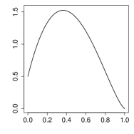
$F_{+}^{\prime}(0)=1$
$F_{+}^{\prime}(0)=1.5$

Figure 3: Beta mixture densities $wB(1,2)+(1-w)B(2,b)$ with $F_{+}^{\prime}(0)=0,0.5,1,1.5$ and $F^{\prime\prime}_{+}(0)=6$ (left column) and $F^{\prime\prime}_{+}(0)=30$ (right column).

	$F^{\prime\prime}_{+}(0)=6$	$F^{\prime\prime}_{+}(0)=30$
$F_{+}^{\prime}(0)=0$
$F_{+}^{\prime}(0)=0.5$
$F_{+}^{\prime}(0)=1$
$F_{+}^{\prime}(0)=1.5$

Figure 4: $\mathrm{MSE}(\alpha)$ for $K^{L}_{q}$, $q=1,2,3$, with $K$ the Epanechnikov kernel, where $F$ is the beta mixture distribution $wB(1,2)+(1-w)B(2,b)$ with $F^{\prime}_{+}(0)=0,0.5,1,1.5$, $F^{\prime\prime}_{+}(0)=6$ (left column) and $F^{\prime\prime}_{+}(0)=30$ (right column). The sample size is $n=50$.

For each one of these test distributions we present in Figure 4 the exact mean square error of $\tilde{F}_{nh}(x)$, for $x=\alpha h$ and $\alpha\in\,]0,1[$, given by

$$\mathrm{MSE}(\alpha)=\mathrm{V}(\alpha)+\mathrm{B}(\alpha)^{2},$$

where

$$n\mathrm{V}(\alpha) :=n\mathrm{Var}\tilde{F}_{nh}(a+\alpha h)=\!\int F(a+(\alpha-u)h)B^{L}(u;\alpha)du-\big{(}\mathrm{E}\tilde{F}_{nh}(a+\alpha h)\big{)}^{2}$$

and

$$\mathrm{B}(\alpha) :=\mathrm{E}\tilde{F}_{nh}(a+\alpha h)-F(a+\alpha h)=\!\int F(a+(\alpha-u)h)K^{L}(u;\alpha)\,du-F(a+\alpha h)$$

(on these expressions see Section 5 below). The global bandwidth $h$ that determines the boundary region was always taken equal to the asymptotically optimal bandwidth $h_{0}$ given in Theorem 2, and we have considered the sample size $n=50$. Similar pictures were generated for sample sizes $n=100$ and $n=200$, but they were not included here to save space. As before, we have taken for $K$ the Epanechnikov kernel.

From the graphics we conclude that the boundary behaviour of the kernel estimator based on the boundary kernels $K^{L}_{q}$, for $q=1,2,3$, is dominated by the magnitude of the underlying density $f=F^{\prime}$ over the boundary region. For large values of $F_{+}^{\prime}(0)$ we see that the boundary kernel $K_{3}^{L}$ is superior to both $K_{1}^{L}$ and $K_{2}^{L}$, being the advantage over the second order boundary kernels bigger for large than for small values of $F_{+}^{\prime\prime}(0)^{2}$. Notice that this latter conclusion is in accordance with the asymptotic comparisons presented in Section 2. Although less performing than $K_{3}^{L}$, the kernel $K_{1}^{L}$ is, in this case, superior to $K_{2}^{L}$. When the underlying density is such that $F_{+}^{\prime}(0)=0$, in which case the classical kernel estimator does not suffer from boundary problems, we see that the boundary kernels $K_{1}^{L}$ and $K_{2}^{L}$ perform similarly being both slightly better than $K_{3}^{L}$. Finally, for intermediate values of $F_{+}^{\prime}(0)$ the three considered left boundary kernels are equally performing. Based on this analysis, we conclude that none of the considered boundary kernels is the best over the considered set of test distributions. However, the kernel $K_{3}^{L}$ shows to be particularly interesting because it is especially performing when the classical boundary kernel estimator suffers from severe boundary problems.

Figure 5: $\mathrm{ISE}$ distributions for the boundary corrected estimators with left boundary kernels $K^{L}_{q}$, $q=1,2,3$, and for the classical estimator with kernel $K$ over the regions $[0,h]$ (left), $[0,1-h]$ (center) and $[0,1]$ (right). $F$ is the beta mixture distribution $wB(1,2)+(1-w)B(2,b)$ with $F^{\prime}_{+}(0)=1.5$ and $F^{\prime\prime}_{+}(0)=6$. The boxplots are based on 500 generated samples of size $n=50$ and $K$ is the Epanechnikov kernel.

We finish this section with a cautionary note that aims to call the attention of the reader to the fact that, due to the continuity of $F$ on $\mathbb{R}$, the boundary effects for kernel distribution function estimation may not have the same impact in the global performance of the estimator as in probability density or regression function estimation frameworks (see Gasser and Müller, 1979). However, one may have cases where the local behaviour dominates the global behaviour of the estimator which stresses the relevance in using boundary corrections for the classical kernel distribution function estimator. We illustrate this fact by taking the above considered beta mixture distribution with $F^{\prime}_{+}(0)=1.5$ and $F^{\prime\prime}_{+}(0)=6$ (see Figure 3). In Figure 5 we present the empirical distribution of the integrated square error of the classical estimator with kernel $K$ and of the boundary corrected estimators with boundary kernels $K^{L}_{q}$, $q=1,2,3$, over the boundary regions $[0,h]$ (left boundary ISE) and $[1-h,1]$ (right boundary ISE), and over the all interval $[0,1]$ (ISE). The boxplots are based on 500 generated samples of size $n=50$. We conclude that the local behaviour of the estimator over the left boundary region has a clear impact on the global performance of the estimator which supports the use of boundary corrections for the classical kernel distribution function estimator.

5 Proofs

We limit ourselves to present the proof of Theorem 1. The proofs of Theorems 2 and 3 follow straightforward from the proofs of the corresponding results given in Tenreiro (2013) and the asymptotic expansions for bias and variance of $\tilde{F}_{nh}(x)$ we present below.

Proof of Theorem 1.a): For $x\in\,]a,a+h[$, the expectation of $\tilde{F}_{nh}(x)$ is given by

$$\mathrm{E}\tilde{F}_{nh}(x) =\int F(x-uh)K^{L}(u;(x-a)/h)\,du,$$

(see Tenreiro, 2013, p. 186). By the continuity of the second derivative of $F$ on $[a,b]$ and Taylor’s formula, we have

$$F(x-uh)=F(x)-uhF^{\prime}(x)+u^{2}h^{2}\int_{0}^{1}(1-t)F^{\prime\prime}(x-tuh)\,dt,$$ (9)

for $-1\leq u\leq(x-a)/h$ , from which we deduce that

$$\mathrm{E}\tilde{F}_{nh}(x)-F(x)-\frac{h^{2}}{2}F^{\prime\prime}(x)\mu_{L}((x-a)/h)=A(x,h)+B(x,h),$$ (10)

where

$$A(x,h) =F(x)\big{(}\mu_{0,L}((x-a)/h)-1\big{)}-hF^{\prime}(x)\mu_{1,L}((x-a)/h)$$

$$\quad+\frac{h^{2}}{2}F^{\prime\prime}(x)((x-a)/h)\mu_{1,L}((x-a)/h),$$

and

$$B(x,h)=h^{2}\iint_{0}^{1}(1-t)\big{(}F^{\prime\prime}(x-tuh)-F^{\prime\prime}(x)\big{)}dt\,u^{2}K^{L}(u;(x-a)/h)\,du,$$

is such that

$$\sup_{x\in\,]a,a+h[}|B(x,h)|\leq\frac{h^{2}}{2}\sup_{\alpha\in\,]0,1[}|\mu_{0,L}|(\alpha)\sup_{y,z\in[a,b]:\,|y-z|\leq h}|F^{\prime\prime}(y)-F^{\prime\prime}(z)|.$$ (11)

On the other hand, taking into account that $F(a)=0$ and using condition (6) and the Taylor’s expansions

$$F(x) =(x-a)F^{\prime}(a)+\frac{1}{2}(x-a)^{2}F^{\prime\prime}(a)$$

$$\quad+(x-a)^{2}\int_{0}^{1}(1-t)\big{(}F^{\prime\prime}(a+(x-a)t)-F^{\prime\prime}(a)\big{)}dt$$ (12)

and

$$F^{\prime}(x)=F^{\prime}(a)+(x-a)F^{\prime\prime}(a)+(x-a)\int_{0}^{1}\big{(}F^{\prime\prime}(a+(x-a)t)-F^{\prime\prime}(a)\big{)}dt,$$ (13)

we get

$$\sup_{x\in\,]a,a+h[}|A(x,h)|\leq h^{2}\sup_{\alpha\in\,]0,1[}|\mu_{0,L}|(\alpha)\sup_{y,z\in[a,b]:\,|y-z|\leq h}|F^{\prime\prime}(y)-F^{\prime\prime}(z)|.$$ (14)

Part a) of Theorem 1 follows now from (10), (11) and (14), and the fact that

$$\sup_{y,z\in[a,b]:\,|y-z|\leq h}|F^{\prime\prime}(y)-F^{\prime\prime}(z)|=o(1). \blacksquare$$

Proof of Theorem 1.b): From Part a), the variance of $\tilde{F}_{nh}(x)$ is given by

$$n\mathrm{Var}\tilde{F}_{nh}(x) =\int\bar{K}^{L}(z;(x-a)/h)^{2}hf(x-uh)dz-\big{(}\mathrm{E}\tilde{F}_{nh}(x)\big{)}^{2}$$

$$=F(x)(1-F(x))+C(x,h)+O\big{(}h^{2}\big{)},$$

uniformly in $x\in\,]a,a+h[$, where

$$C(x,h)=\int\bar{K}^{L}(u;(x-a)/h)^{2}hf(x-uh)du-F(x).$$

Moreover, using (9) and the fact that

$$\lim_{u\rightarrow-\infty}\bar{K}^{L}(u;\alpha)=0\quad\mbox{and }\lim_{u\rightarrow+\infty}\bar{K}^{L}(u;\alpha)=\mu_{0,L}(\alpha),\mbox{ for }\alpha\in\,]0,1[,$$

we deduce that

$$C(x,h) =\int F(x-zh)B^{L}(z;(x-a)/h)dz-F(x)$$

$$=F(x)\big{(}\mu_{0,L}((x-a)/h)^{2}-1\big{)}-hF^{\prime}(x)m_{1,L}((x-a)/h)$$

$$\quad+h^{2}\iint_{0}^{1}(1-t)F^{\prime\prime}(x-tuh)dtu^{2}B^{L}(u;(x-a)/h)du$$

$$=F(x)\big{(}\mu_{0,L}((x-a)/h)^{2}-1\big{)}-hF^{\prime}(x)m_{1,L}((x-a)/h)+O(h^{2}),$$ (15)

uniformly in $x\in\,]a,a+h[$, as $\sup_{\alpha\in\,]0,1[}\int|u^{2}B^{L}(u;\alpha)|du<\infty$.

Finally, from (15) and Taylor’s expansions (5) and (13) we get

$$\sup_{x\in\,]a,a+h[}\left|C(x,h)+h\,F^{\prime}(x)\nu_{L}\big{(}(x-a)/h\big{)}\right|=O(h^{2}),$$

which concludes the proof. $\blacksquare$

Acknowledgments. Research partially supported by Centro de Matemática da Universidade de Coimbra (funded by the European Regional Development Fund through the program COMPETE and by the Portuguese Government through the FCT–Fundação para a Ciência e Tecnologia under the project PEst-C/MAT/UI0324/2011).

References

• Chacón, Monfort and Tenreiro (2014) Chacón, J.E., Monfort, P., Tenreiro, C. (2014). Fourier methods for smooth distribution function estimation. Statist. Probab. Lett. 84, 223–230.
• Chacón and Rodríguez-Casal (2010) Chacón, J.E., Rodríguez-Casal, A. (2010). A note on the universal consistency of the kernel distribution function estimator. Statist. Probab. Lett. 80, 1414–1419.
• Gasser and Müller (1979) Gasser, T., Müller, H.-G. (1979). Kernel estimation of regression functions. In Smoothing techniques for curve estimation (T. Gasser and M. Rosenblatt, Eds.), Lecture Notes in Mathematics 757, 23–68.
• Gasser et al. (1985) Gasser, T., Müller, H.-G., Mammitzsch, V. (1985). Kernels for nonparametric curve estimation. Journal of the Royal Statistical Society. Series B. Methodological 47, 238–252.
• Giné and Nickl (2009) Giné, E., Nickl, R. (2009). An exponential inequality for the distribution function of the kernel density estimator, with applications to adaptive estimation. Probab. Theory Related Fields 143, 569–596.
• Jones (1990) Jones, M.C. (1990). The performance of kernel density functions in kernel distribution function estimation. Statis. Probab. Lett. 9, 129–132.
• Mason and Swanepoel (2011) Mason, D.M., Swanepoel, J.W.H. (2011). A general result on the uniform in bandwidth consistency of kernel-type function estimators. TEST 20, 72–94.
• Müller (1991) Müller, H.-G. (1991). Smooth optimum kernel estimators near endpoints. Biometrika 78, 521–530.
• Nadaraya (1964) Nadaraya, E.A. (1964). Some new estimates for distribution functions. Theory Probab. Appl. 9, 497–500.
• R Development Core Team (2011) R Development Core Team (2011). R: A Language and Environment for Statistical Computing. R Foundation for Statistical Computing, Vienna, Austria. URL http://www.R-project.org
• Rice (1984) Rice, J. (1984). Boundary modification for kernel regression. Communications in Statistics – Theory and Methods 13, 893–900.
• Tenreiro (2013) Tenreiro, C. (2013). Boundary kernels for distribution function estimation. REVSTAT–Statistical Journal 11, 169–190.
• Tiago de Oliveira (1963) Tiago de Oliveira, J. (1963). Estatística de densidades: resultados assintóticos. Rev. Fac. Ciên. Lisboa 9, 111–206.
• Wand and Jones (1995) Wand, M.P., Jones, M.C. (1995). Kernel Smoothing. London: Chapman & Hall.
• Watson and Leadbetter (1964) Watson, G.S., Leadbetter, M.R. (1964). Hazard analysis II. Sankhyā Ser. A 26, 101–116.
• Winter (1973) Winter, B.B. (1973). Strong uniform consistency of integrals of density estimators. Canad. J. Statist. 1, 247–253.
• Winter (1979) Winter, B.B. (1979). Convergence rate of perturbed empirical distribution functions. J. Appl. Probab. 16, 163–173.
• Yamato (1973) Yamato, H. (1973). Uniform convergence of an estimator of a distribution function. Bull. Math. Statist. 15, 69–78.