Inverted approach to the inverse scattering problem: complete solution of the Marchenko equation for a model system

Abstract

An example of full solution of the inverse scattering problem on the half line (from 0 to $\infty$) is presented. For this purpose, a simple analytically solvable model system (Morse potential) is used, which is expected to be a reasonable approximation to a real potential. First one calculates all spectral characteristics for the fixed model system. This way one gets all the necessary input data (otherwise unobtainable) to implement powerful methods of the inverse scattering theory. In this paper, the multi-step procedure to solve the Marchenko integral equation is described in full details. Excellent performance of the method is demonstrated and its combination with the Marchenko differential equation is discussed. In addition to the main results, several important analytic properties of the Morse potential are unveiled. For example, a simple analytic algorithm to calculate the phase shift is derived.

I Introduction

Strict mathematical criteria for the unique solution of the one-dimensional inverse scattering problem have been formulated long ago, thanks to the outstanding contributions by many researchers Levinson1 ; Levinson2 ; Bargmann1 ; Bargmann2 ; GL ; Jost1 ; Jost2 ; Marchenko1 ; Marchenko2 ; Krein1 ; Krein2 (see Chadan for a historical overview). However, in spite of the perfect consistency and mathematical beauty of the concept, these rigorous criteria have rarely been used in practice, because the necessary input data are very difficult to obtain. Indeed, one has to know the full energy spectrum of the bound states $E_{n}<0$ ($n=0,1,2,...,N-1$) and the full energy dependence (from 0 to $\infty$) of the phase shift $\delta(E)$ for the scattering states ($E>0$). Even if the mentioned obligatory requirements were fulfilled (which is never the case), this would only be sufficient to construct an $N$-parameter family of phase-equivalent and isospectral potentials. One has to somehow fix $N$ additional parameters, the so-called norming constants, in order to ascertain the potential uniquely.

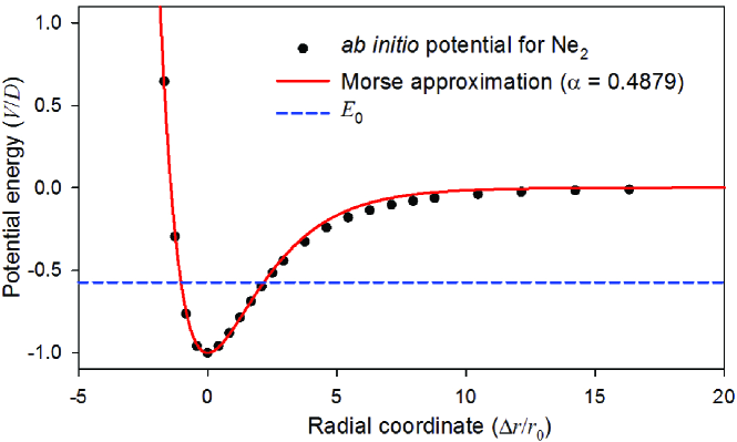
Figure 1: An illustration to the physical background of the proposed approach.

On the other hand, the shape of a real potential is not arbitrary, but often it looks like the curve in Fig. 1. In this figure, a comparison is made between an ab initio potential for Ne₂ molecule NePot and its Morse approximant, calculated according to the formula Morse29

$$\frac{V(r)}{D}=\exp\left[-\frac{2\alpha\left(r-R_{e}\right)}{r_{0}}\right]-2\exp\left[-\frac{\alpha\left(r-R_{e}\right)}{r_{0}}\right],$$ (1)

taking $D=42.153$ K NePot ; Merkt and $R_{e}=3.0895$ Å NePot . The Morse curve in Fig. 1 was calculated with $r_{0}\equiv\sqrt{\hbar^{2}/(2mD)}=0.2388$ Å, $\alpha=0.4879/r_{0},$ and $\Delta r\equiv r-R_{e}$. It has only one bound state: $E_{0}/D=-0.5716,$ and practically the same value has been determined for the single discrete level of the Ne₂ molecule, both theoretically NePot and experimentally Merkt .

Fig. 1 was presented for illustrative purposes, to continue the above discussion. Namely, in principle, the unknown norming constants for a real potential can be treated as variational parameters. One may try to guess their correct values by fitting to Eq. (1). Moreover, one might even think about using this simple model potential to examine different solution schemes of the inverse scattering theory, and this is the main idea developed in this paper. Morse potential has many unique analytic properties, which makes it especially suitable for modelling. In particular, for this model system one can ascertain all the necessary spectral characteristics to any desired accuracy. Thereafter, one can use them as input data, instead of getting these data from real experiments.

The idea to invert an inverse problem is, of course, tautological but not at all meaningless. Indeed, despite the immense computational power which is now available to the researchers, one hardly could find any example of complete solution of the inverse scattering problem on the half line. The main reason for this deficiency is the lack of the necessary input data, and consequently, there seems to be no motivation to perform such studies. Then, what is the motivation for the present study? First of all, in author’s opinion there is a debt of honor to be paid to the researchers who developed this beautiful theory. Nowadays people tend to consider the inverse scattering a ’pedagogical’ problem which is of little scientific interest. Unfortunately, such an ignorant view is not based on the real knowledge, but is a mere belief. Implementation of the methods of the inverse scattering theory is not at all a trivial task. On the contrary, this is a complex and computationally demanding multi-step procedure which has to be performed with utmost accuracy. In this paper, we are going to describe this procedure for a very simple model system, to make it understandable for a wide audience of potential readers. This can be considered a first step towards the real implementation of the method. Another, more specific motive for this work is the obvious need to clarify some conceptual details, as will be explained in Sec. II.

Performing an applicability test of the Marchenko method is not the only issue addressed in this paper. In author’s opinion, the model system itself deserves special attention. Useful properties of the Morse potential, as well as the solution to the related Schrödinger equation already given by Philip Morse himself Morse29 , are well known to physicists. Since the potential is shape-invariant, this solution can even be found by pure algebraic means, using the Gendenshtein’s recipe Gendenshtein . However, in this context we are talking about the physically correct linear combination of the two special solutions to the Schrödinger equation. There are lots of systems which can be analyzed in exactly the same way (the simplest one is the harmonic oscillator), but within this pattern the feature which makes Morse potential really unique is overlooked. Namely, for a Morse potential the two linearly independent solutions to the Schrödinger equation can always be easily ascertained analytically (even if $D<0$!). This is not the case for a harmonic oscillator or any other popular model system.

Consequently, the approach based on Eq. (1) is not just an option among many others, but it is often the most appropriate choice for modelling a real quantum system. Moreover, one may construct a more reliable model consisting of several Morse-type components, still preserving the exact solubility of the Schrödinger equation. Such technically rather complex developments are not analyzed in this paper (see, e.g., Selg2001 and SelgJCP for more details), because here we concentrate on solving the inverse not the direct Schrödinger problem. For this reason, the model has been chosen to be as simple as possible.

Nevertheless, as a matter of fact, the scattering properties of the Morse potential have not found much attention so far, and there still is some work to do. In Sec. III, a simple analytic formula for calculating the phase shift is derived. Unexpectedly, in addition to this specific result, there is a pure mathematical outcome which is directly related to Eq. (1). Namely, a very accurate algorithm for evaluating the Riemann-Siegel function (see Edwards ) was obtained, as a kind of bonus for calculating the phase shift.

The remaining parts of the paper are organized as follows. The details of calculating the kernel of the Marchenko equation are described in Sec. IV and the solution method itself is under examination in Sec. V. Finally, Sec. VI concludes the work.

II Marchenko integral equation

The basis for this paper is the integral equation

$$A(r,t)=A_{0}(r+t)+\int\limits_{r}^{\infty}A(r,s)A_{0}(s+t)ds,\ t\geq r,$$ (2)

derived by Marchenko Marchenko1 . The Marchenko method is preferred, because the kernel of Eq. (2) is directly related to the main spectral characteristics of the system, while an alternative approach, the Gelfand-Levitan method GL , requires an additional calculation of the Jost function.

The kernel of Eq. (2) reads

$$A_{0}(x)=\frac{1}{2\pi}\int\limits_{-\infty}^{\infty}\left[S(k)-1\right]\exp(ikx)dk-\sum_{n}s_{n}^{2}\exp(-\gamma_{n}x),$$ (3)

$$k\equiv\sqrt{E/C},\ \gamma_{n}\equiv\sqrt{-E_{n}/C},\ S(k)\equiv\exp\left[2i\delta(k)\right],$$

where $C\equiv\hbar^{2}/(2m)$ and $s_{n}$ are the norming constants for the Jost solution of the related Schrödinger equation:

$$f(i\gamma_{n},r)=\exp(-\gamma_{n}r)+\int\limits_{r}^{\infty}A(r,x)\exp(-\gamma_{n}x)dx,$$ (4)

so that $f(i\gamma_{n},r)\rightarrow\exp(-\gamma_{n}r)$ as $r\rightarrow\infty$, and

$$s_{n}^{2}\int\limits_{0}^{\infty}\left[f(i\gamma_{n},r)\right]^{2}dr=1.$$ (5)

If one is able to solve Eq. (2) then the potential can be easily determined:

$$V(r)=-2C\frac{dA(r,r)}{dr}.$$ (6)

The key formulas were given in full detail, in order to clarify the issue mentioned above. Namely, in several highly appreciated overviews either the Marchenko equation itself or its kernel or both of them are given incorrectly (see Refs. Chadan1, , p. 73; Chadan, , p. 79; Chadan2, , p. 732; Chadan3, , p. 178). The dispute concerns the sign of the second term in Eq. (3), which is ’plus’ in all these overviews. According to Marchenko’s original works (see, e.g., Refs. AgrMarch, , p. 62; Marchenko, , p. 218), on the contrary, there should be ’minus’ as in Eq. (3), and this is definitely true. Indeed, the original Marchenko equation can be rewritten as

$$A(r,t) = -B_{0}(r+t)-\int\limits_{r}^{\infty}A(r,s)B_{0}(s+t)ds,$$

$$B_{0}(x) = \frac{1}{2\pi}\int\limits_{-\infty}^{\infty}\left[1-S(k)\right]\exp(ikx)dk+\sum_{n}s_{n}^{2}\exp(-\gamma_{n}x).$$

Consequently, taking $A_{0}(x)\equiv-B_{0}(x)$, one comes to Eqs. (2)-(3). Most likely, the wrong sign given in Refs. Chadan, , Chadan1, -Chadan3, is just a human error. However, it is misleading (especially in the pedagogical context) and should be corrected. On the other hand, it is quite surprising that this error has not even been noticed until now. Indirectly, it means that no one has attempted to put the Marchenko method into practice, which provides another motivation for the present study.

Let us specify the problem and the scheme for its solution. First, one calculates the spectral characteristics for a simple model potential described by Eq. (1). Then one determines the kernel of the Marchenko equation according to Eq. (3). Finally, one solves Eq. (2) and calculates the related potential according to Eq. (6). If the procedure is successful then the initial potential is recovered. Throughout this paper, dimensionless units for the energy and radial coordinate will be used, taking $r_{0}\equiv\sqrt{\hbar^{2}/(2mD)}=1,$ $D=1,$ and consequently, $C=1.$

For a Morse potential, the norming constants $s_{n}$ can be easily ascertained analytically. Let us fix, for example, $\alpha=2/3.$ Then the system has only one bound state:

$$E_{n}=-D(1-\frac{n+1/2}{a})^{2}\rightarrow E_{0}=-D(1-\frac{1}{2a})^{2},$$ (7)

where $a\equiv\sqrt{D/C}/\alpha.$ Consequently, in our unit system, $a=1/\alpha$ and $\gamma_{0}=2/3=\alpha.$ Therefore, this particular case is especially suitable for illustrative purposes and only this case will be examined further on. (The same approach, with minor adjustments concerning the different values for $\alpha$ and $\gamma_{0}$, can be applied to the model potential shown in Fig. 1). To conclusively fix the model, let us assume that the minimum of the potential is located at $R_{e}=2.5r_{0}$.

At first sight it may seem that the system has another level exactly at the zero point. Indeed, if one takes $\alpha=2/3$ then $a=3/2$ and, according to Eq. (7), $E_{1}=0$. Actually, however, this is not the case, because the coordinate here ranges from 0 to $\infty$, not from $-\infty$ to $\infty$ as for a classical Morse oscillator. Therefore, as can be easily proved, the possible additional level is shifted slightly above (not below) the dissociation limit, becoming a scattering state. Another nuance is that, strictly speaking, one should form a linear combination of both solutions of the Schrödinger equation, to fix the correct regular solution. Again, it can be shown (see, e.g., Selg2006 ) that the second special solution is of next to no importance, so that the physical solution reads

$$\Psi_{0}=N_{0}\exp(-y/2)y$$ (8)

as in the ’normal’ Morse case. Here $N_{0}$ is the related norming constant and a new dimensionless coordinate $y\equiv 2a\exp\left[-\alpha\left(r-R_{e}\right)\right]$ was introduced.

The parameter $N_{0}$ as well as the norming constant for the Jost solution (4) can be easily determined:

$$s_{0}^{2}=\frac{y_{0}^{2}\alpha}{1-\int\limits_{y_{0}}^{\infty}\exp(-y)ydy},\ y_{0}\equiv 2a\exp\left(\alpha R_{e}\right).$$ (9)

The second term in the denominator is negligible, so that, to a high accuracy, $s_{0}^{2}=y_{0}^{2}\alpha=6\exp(10/3)$. This is the value which we are trying to recover. However, to clarify the sign problem described above, the quantity $s_{0}^{2}$ will be treated as a variational (not definitely positive!) parameter. We will see that its expected value is indeed the correct value.

III Phase shift for the Morse potential

Let us see how to determine the full energy dependence of the phase shift, subjected to a strong constraint

$$\delta(0)-\delta(\infty)=N\pi$$ (10)

($N=1$ in our case), according to the Levinson theorem Levinson1 ; Levinson2 . The analytic background of the problem has been described elsewhere SelgJCP (see Eqs. (23) to (29) there). There are several formally equivalent approaches to building the regular solution of the Schrödinger equation for a scattering state. For example, we may proceed from Eq. (25) of Ref. SelgJCP, . Then, after some analytical work, we get the following special solutions:

$$\Psi_{1}(k,r) = \left|S\left(a,i\beta;y\right)\right|\cos\left\{\alpha_{0}+\arg\left[S\left(a,i\beta;y\right)\right]-kr\right\},$$ (11)

$$\Psi_{2}(k,r) = \left|S\left(a,i\beta;y\right)\right|\sin\left\{\alpha_{0}+\arg\left[S\left(a,i\beta;y\right)\right]-kr\right\},$$

with

$$S(a,i\beta;y) = \sum_{n=0}^{\infty}B_{n},B_{0}=1,B_{1}=-\frac{ay}{2i\beta+1},\ \beta\equiv k/\alpha,$$

$$\ B_{n} = \frac{y}{n(2i\beta+n)}(-aB_{n-1}+\frac{y}{4}B_{n-2}),\ n=2,3,...,$$ (12)

$$\alpha_{0}\equiv\beta\ln(2a)+\beta_{N}-B+kR_{e},$$ (13)

$\beta_{N}\equiv\arg\left[\left(i\beta+1\right)\left(i\beta+2\right)...\left(i\beta+N\right)\right]$, and

$$B\equiv\arg\left[\frac{\Gamma(2i\beta)}{\Gamma(i\beta)}\right],$$ (14)

($N=1$ in our case), $\Gamma$ being the gamma function.

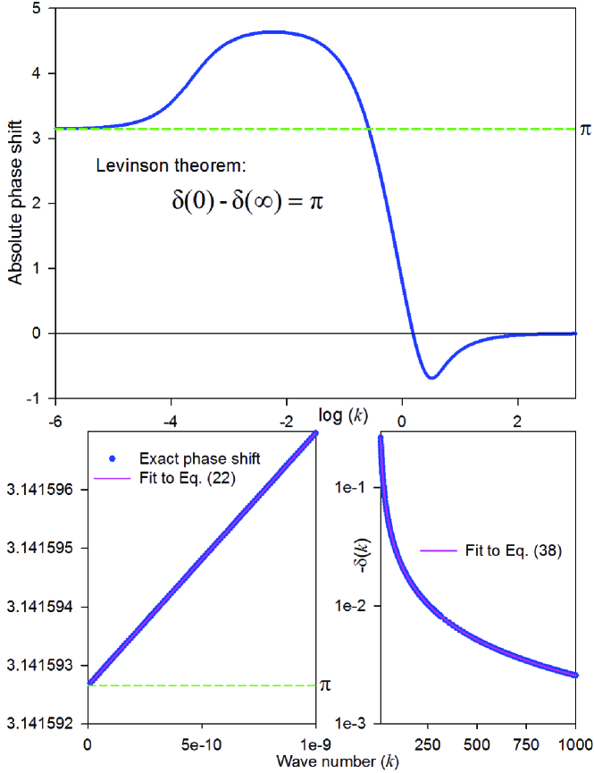
Figure 2: Phase shift for the potential Eq. (1) depending on the wave number (parameters are specified in Sec. II). Lower graphs demonstrate the asymptotic behavior of $\delta(k)$.

Figure 3: Wave functions for the scattering states at extremely small energies. The same set of wave functions is shown in all graphs and their insets, but note that the coordinate ranges are essentially different.

From the regularity requirement $\Psi(0)=A_{1}\Psi_{1}(0)+A_{2}\Psi_{2}(0)=0,$ one gets the ratio of the coefficients

$$\frac{A_{1}}{A_{2}}=-\tan\left[\alpha_{0}+\arg\left(S_{0}\right)\right],\ S_{0}\equiv S\left(a,i\beta;y_{0}\right).$$ (15)

On the other hand, since $S(a,i\beta;y)\rightarrow 1$ as $r\rightarrow\infty$ SelgJCP , one gets a formula for the phase shift:

$$\tan\left[\delta(k)\right]=\frac{\frac{A_{1}}{A_{2}}\cos\alpha_{0}+\sin\alpha_{0}}{\frac{A_{1}}{A_{2}}\sin\alpha_{0}-\cos\alpha_{0}},$$ (16)

and consequently, a general expression for the wave function $\Psi=A_{1}\Psi_{1}+A_{2}\Psi_{2}$ (for simplicity we drop the arguments of the $S$-functions)

$$\Psi(k,r)=-\frac{A_{2}\left|S\right|}{\cos\left[\alpha_{0}+\arg\left(S_{0}\right)\right]}\sin\left[kr+\arg\left(S_{0}\right)-\arg\left(S\right)\right].$$

The last formula is valid for any $r$, and also in the limit $r\rightarrow\infty$. From this one immediately concludes that $A_{2}=-\cos\left[\alpha_{0}+\arg\left(S_{0}\right)\right]$ and $A_{1}=\sin\left[\alpha_{0}+\arg\left(S_{0}\right)\right],$ which means that

$$\Psi(k,r)=\left|S\right|\sin\left\{kr+\arg\left(S_{0}\right)-\arg\left(S\right)\right\},$$ (17)

and most importantly,

$$\delta(k)=\arg\left(S_{0}\right).$$ (18)

This is the simple formula mentioned in Sec. I. Combined with Eq. (12), it enables to easily ascertain the phase shift for any scattering state and thus, its full dependence on energy (or wave number). The result for the specified Morse potential is shown in Fig. 2 (main graph). Note that the k-scale there is logarithmic, so that the figure involves 18 orders of magnitude in the energy space. Full agreement with the Levinson theorem (10) can be seen as well.

Fig. 3 demonstrates the behavior of the scattering wave functions as $E\rightarrow 0.$ In general, the wave functions can be calculated using Eqs. (12), (17) and (18). Note, however, that the $S$-functions are defined as Selg2001

$$S(a,c;x)\equiv\exp(-x/2)\Phi(-a+c+1/2,2c+1;x),$$ (19)

where

$$\Phi(a,c;x)=1+\frac{ax}{1!c}+\frac{a(a+1)x^{2}}{2!c(c+1)}+....$$ (20)

Therefore, if $E\rightarrow 0$ and consequently, $i\beta\rightarrow 0$, then it is more appropriate to explicitly use Eq. (20). As a result, one gets the following rapidly converging expression:

$$S(a,i\beta;y)=\exp(-y/2)\left\{1-y+i\beta y\left[3-\frac{0!}{\left(2!\right)^{2}}y-\frac{1!}{\left(3!\right)^{2}}y^{2}-\frac{2!}{\left(4!\right)^{2}}y^{3}-...\right]\right\},$$

which was actually used to compose Fig. 3.

As the energy is extremely low, linear coordinate dependence can be seen in a wide region, which is in full agreement with the well-known rule

$$\delta(k)=N\pi-\arctan(ka_{0}),$$ (21)

where $a_{0}$ is the scattering length. From Eqs. (17), (18) and (21) it follows that

$$\Psi(k,r)\rightarrow\sin\left[kr+\delta(k)\right]\rightarrow\sin\left(kr\right)+\tan\left[\delta(k)\right]\rightarrow k\left(r-a_{0}\right),$$

and this is indeed the case, while $a_{0}=-4312.06224.$

Practically the same scattering length is obtained from the real k-dependence of the phase shift (see the lower left graph in Fig. 2), using Eqs. (12), (18) and (19)-(21).

III.1 An algorithm for the Riemann-Siegel function

Usually, to calculate $\delta(k)$ there is no need to make any use of Eqs. (13)-(14). In some special cases, however, the convergence of the series (12) may be slow. Then it may be appropriate to combine Eqs. (25) and (28) from Ref. SelgJCP, . As a result, again after some analytical work, one comes to the following expression:

$$\tan\left[\alpha_{0}+\arg\left(S\right)\right]=\frac{\alpha_{N}^{2}\beta}{y^{2N+1}}\exp(y)F\left(N,i\beta;y\right),$$ (22)

where $\alpha_{N}\equiv\left|\left(i\beta+1\right)\left(i\beta+2\right)...\left(i\beta+N\right)\right|,$

$$F\left(N,i\beta;y\right)\equiv\frac{1-\frac{N^{2}+\beta^{2}}{1!y}+\frac{\left(N^{2}+\beta^{2}\right)\left[\left(N-1\right)^{2}+\beta^{2}\right]}{2!y^{2}}+...}{1+\frac{\left(N+1\right)^{2}+\beta^{2}}{1!y}+\frac{\left[\left(N+1\right)^{2}+\beta^{2}\right]\left[\left(N+2\right)^{2}+\beta^{2}\right]}{2!y^{2}}+...},$$ (23)

and we assumed that $N=a-1/2$.

To exploit Eqs. (22)-(23), one takes $y=y_{0}$, uses Eq. (13), and finally gets the phase shift according to Eq. (18). The only problem is how to ascertain the parameter $B$ defined by Eq. (14). Fortunately, we can apply to the theory of gamma functions (see Bateman , Sec. 1.2):

$$\Gamma(1/2+z)\Gamma(1/2-z)=\frac{\pi}{\cos\left(\pi z\right)},$$

$$\Gamma(2z)=\frac{2^{2z-1}}{\sqrt{\pi}}\Gamma(z)\Gamma(1/2+z)=\frac{2^{2z-1}\sqrt{\pi}}{\cos\left(\pi z\right)}\cdot\frac{\Gamma(z)}{\Gamma(1/2-z)}.$$ (24)

Taking here $2z=1/2+i\beta$, one easily gets the desired result:

$$B=\arg\left[\frac{\Gamma(2i\beta)}{\Gamma(i\beta)}\right]=\arg\left[\Gamma(i\beta+1/2)\right]+2\beta\ln 2=\beta\ln\left(8\pi\right)+\arctan\left[\tanh\left(\frac{\beta\pi}{2}\right)\right]+2\theta(\beta),$$ (25)

where

$$\theta(\beta)\equiv\arg\left[\Gamma(1/4+i\beta/2)\right]-\beta/2\ln\pi$$ (26)

is the Riemann–Siegel theta function, whose behavior is well known as $\beta\rightarrow 0$ or $\beta\rightarrow\infty.$ Namely Edwards ,

$$\beta\rightarrow 0:\theta(\beta)=-\frac{\beta}{4}\left[2\gamma+\pi+2\ln\left(8\pi\right)\right]+\frac{\beta^{3}}{24}\left[\pi^{3}+28\zeta(3)\right]-\beta^{5}\left[\frac{\pi^{5}}{96}+\frac{31\zeta(5)}{10}\right]+...$$ (27)

and

$$\beta\rightarrow\infty:\theta(\beta)=-\frac{\beta}{2}\ln\left(\frac{2\pi}{\beta}\right)-\frac{\beta}{2}-\frac{\pi}{8}+\frac{1}{48\beta}+\frac{7}{5760\beta^{3}}+\frac{31}{80640\beta^{5}}+...$$ (28)

Here $\gamma=0.5772156649...$ is the Euler-Mascheroni constant and $\zeta(3)=1.2020569032...,\zeta(5)=1.0369277551...$ are the corresponding values of the Riemann zeta function. In practice, Eq. (27) can be used if $\beta<0.1,$ while Eq. (28) is recommended for $\beta>20$. For the intermediate region $\beta\in\left[0.1,20\right]$ an innovation can be introduced. Namely, combining Eq. (25) with a useful formula for calculating $\arg\left[\Gamma(i\beta+1/2)\right]$ Chebotarev , we get

$$2\theta(\beta)=\beta\left[\ln\left(\frac{\sqrt{(1+4\beta^{2})}}{4\pi}\right)-1\right]-\arctan\left[\tanh\left(\frac{\beta\pi}{2}\right)\right]-\frac{I(\beta)}{2},$$ (29)

where Selg2001

$$I(\beta)\equiv\int\limits_{0}^{\infty}\left(\coth t-\frac{1}{t}\right)e^{-t}\sin(2\beta t)\frac{dt}{t}=\int\limits_{0}^{T}e^{-t}\sin(\pi\frac{t}{T})f(t)dt,\qquad T=\frac{\pi}{2\beta},$$

$$f(t)=\frac{\coth t-\frac{1}{t}}{t}-e^{-T}\frac{\coth(t+T)-\frac{1}{t+T}}{t+T}+e^{-2T}\frac{\coth(t+2T)-\frac{1}{t+2T}}{t+2T}-...$$

The integral $I(\beta)$ can be conveniently evaluated numerically or even analytically Selg2003 :

$$I(\beta)=\sum_{n=1}^{\infty}I_{n},I_{n}=\frac{(-1)^{n-1}2^{2n}B_{n}}{(2n)(2n-1)(1+4\beta^{2})^{2n-1}}\sum_{k=0}^{n-1}(-1)^{k}\left(\begin{array}[]{c}2n-1\\ 2k+1\end{array}\right)(2\beta)^{2k+1}.$$ (30)

Here $B_{n}$ denotes the $n$-th order Bernoulli number ($B_{1}=1/6,$ $B_{2}=1/30,$ etc.).

Thus, returning to the main subject of this section, we have found another option for calculating the phase shift, based on Eqs. (18), (13), (22), (25) and (29)-(30):

$$\delta(k)=\arctan\left[\frac{F_{0}\alpha_{N}^{2}\beta\exp(y_{0})y_{0}^{-(2N+1)}-\tan(\alpha_{0})}{1-\tan\left(\alpha_{0}\right)}\right],\ F_{0}\equiv F\left(N,i\beta;y_{0}\right).$$ (31)

This little excursion once again demonstrates wonderful analytic properties of the Morse potential, providing an instructive example how purely physical considerations may lead to a pure mathematical result.

IV Scattering part of the kernel

As the necessary spectral data are now available, we can start solution of the inverse problem. First step is to perform the Fourier transform to fix the scattering part of the kernel (3):

$$A_{s}(x)\equiv\frac{1}{2\pi}\int\limits_{-\infty}^{\infty}\left[S(k)-1\right]\exp(ikx)dk=-\frac{f(x)+g(x)}{\pi},$$ (32)

$$f(x)\equiv\int\limits_{0}^{\infty}\sin\left[2\delta(k)\right]\sin(kx)dk,\ g(x)\equiv 2\int\limits_{0}^{\infty}\sin^{2}\left[\delta(k)\right]\cos(kx)dk.$$ (33)

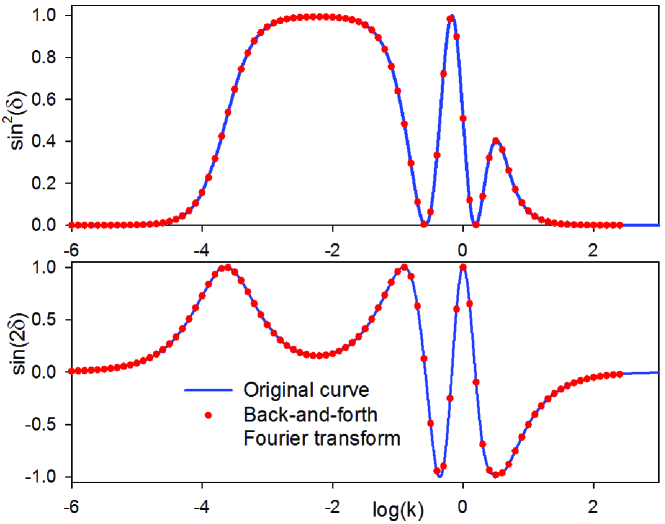
Figure 4: Demonstration of the excellent accuracy of the Fourier transforms performed according to Eqs. (32)-(34).

It can be shown that $A_{s}(-x)=\left[f(x)-g(x)\right]/\pi,$ so that the inverse Fourier transform would result in the following formulas:

$$\sin^{2}\left[\delta(k)\right]=\frac{1}{\pi}\int\limits_{0}^{\infty}g(x)\cos(kx)dx,\ \sin\left[2\delta(k)\right]=\frac{2}{\pi}\int\limits_{0}^{\infty}f(x)\sin(kx)dx.$$ (34)

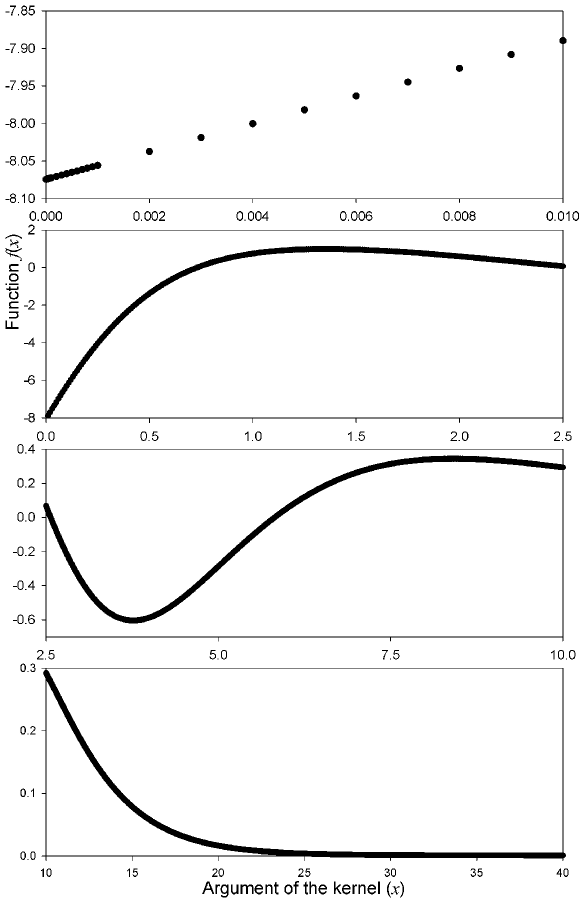
Figure 5: Coordinate dependence of the function $f(x)$ calculated according to Eq. (33).

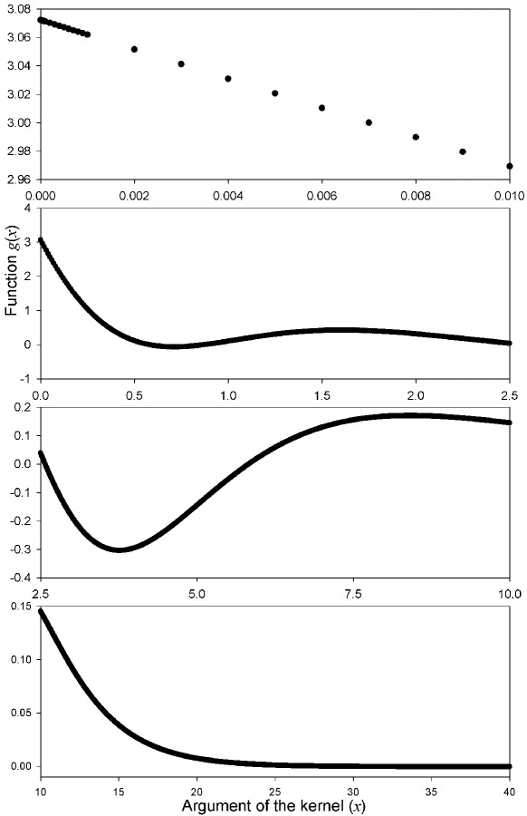
Figure 6: Coordinate dependence of the function $g(x)$ calculated according to Eq. (33).

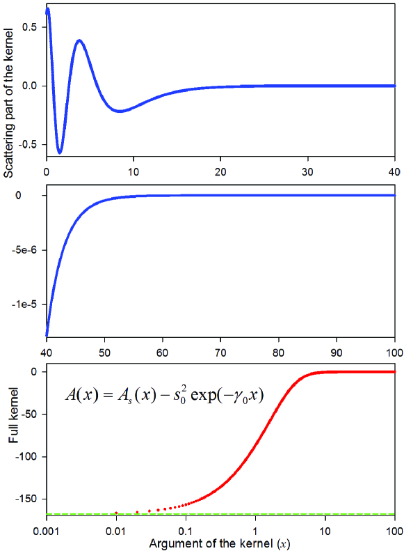
Figure 7: Coordinate dependence of the scattering part of the kernel according to Eq. (3) (two upper graphs) and the full kernel for the examined Marchenko equation (bottom graph).

Calculations according to Eqs. (32)-(33) represent the most challenging part of the overall procedure, because the functions $f(x)$ and $g(x)$ must be ascertained in a wide range with an extreme accuracy. It means, in particular, that the fast Fourier transform techniques are useless for our purposes. Fortunately, one can use an asymptotic formula Selg2006

$$\delta(k)=\frac{a_{1}}{k}+\frac{a_{3}}{k^{3}}+\frac{a_{5}}{k^{5}}+...,\qquad k\rightarrow\infty,$$ (35)

where the coefficients $a_{1},a_{3},a_{5},...$ are directly related to the potential and its derivatives (for example, $a_{1}=-(2C)^{-1}\int\limits_{0}^{\infty}V(r)dr$). Thus the asymptotic part of the integrals (33) can be calculated analytically. In addition, one can make use of the Filon’s quadrature formulas (see Ref. AbrSteg, , p. 890), which are perfectly suitable if $x$ is large. The Filon’s formulas have been used for the range $k\in\left[20,100\right]$ when $x\geq 20,$ while for $x<20$ a more common (but very accurate) approach was used. Namely, the domain was divided into sufficiently small intervals where 64-point Gauss-Legendre quadrature formula is appropriate to the purpose.

The described procedure ensures the correct asymptotic behavior of both functions defined in Eq. (33). Namely,

$$f(x)\approx\frac{\pi}{4}y_{0}\exp(-\frac{\alpha x}{2})+b\exp(-cx),\ g(x)\approx\frac{\pi}{4}y_{0}\exp(-\frac{\alpha x}{2})-b\exp(-cx),$$ (36)

where $b=7.252681534782$e-4, $c=2.315574387346$e-4 are some characteristic constants. Quite remarkably, these formulas hold to better than 10^-10 accuracy for $x\geq 30.$ The second terms in Eq. (36) are not important for the following analysis, since they mutually compensate each other. On the other hand, without these additional terms one cannot correctly perform the inverse Fourier transform according to Eq. (34). In fact, there is no need for this inverse transform as well, but it is recommended, to be sure that the calculated functions $f(x)$ and $g(x)$ are reliable. Fig. 4 demonstrates that this is indeed the case.

Figures 5, 6 and 7 give more detailed information about the solution procedure. (Although the curves in these figures may look like solid lines, they are assemblies of dots which represent the actual results of calculations). Looking at Figs. 5-7, one can understand why the utmost accuracy is needed in performing the Fourier transform. This is most clearly seen in the lowest graph of Fig. 7 (the green dashed line there shows $A(0)$). Indeed, if the Fourier transform is not sufficiently correct then the important information about the scattering properties of the system (shown in figures 5, 6 and in the two upper graphs of Fig. 7) may easily be lost against the background of the bound states’ contribution to the kernel, which dominates at small values of the argument. Thus the whole procedure would become meaningless.

As the result of the Fourier transform according to Eq. (33), one gets two smooth functions that can be very accurately (with absolute error less than 10^-6) approximated by piecewise rational functions

$$\left\{\begin{array}[]{c}f(x)\\ g(x)\end{array}\right.=\frac{a+bx+cx^{2}+dx^{3}+ex^{4}+fx^{5}}{1+gx+hx^{2}+ix^{3}+jx^{4}+kx^{5}+lx^{6}},$$

whose parameters are given in Tables 1 and 2. Using these parameters and applying Eq. (36) for larger arguments, one can reproduce all curves shown in Figs. 5-7.

Table 1: The fitting parameters for the curves shown in Fig. 5.

	Parameters of the rational fit for the function $f(x)$
	$0\leq x\leq 0.2$	$0.2<x\leq 2.5$	$2.5<x\leq 10$	$10<x\leq 30$
$a$	-8.0742834752365	-8.07451927770804	0.710177479533	-1.318246783662
$b$	-139.70663281	21.09396832161	0.078971528944	0.350978767195
$c$	-1964.01791531	-20.103272203664	-0.276506389451	-0.025997992558
$d$	9295.18176575	10.475159850219	0.065047583073	8.813724334413e-4
$e$	-8951.34532192	-2.595277468302	-4.695098041353e-3	-1.492795622311e-5
$f$	0	0.196451244097	1.138463611195e-4	1.117794694102e-7
$g$	19.59774821	-0.316168857071	-0.711060782617	-0.345296699762
$h$	287.27716444	0.804977555407	0.277492349329	0.068087218353
$i$	-511.76899191	-0.412291982417	-0.053313022152	-6.848766446371e-3
$j$	-357.91228265	0.355627589898	6.620633459645e-3	4.849331544015e-4
$k$	-747.01469965	-0.117132459825	-3.875251671984e-4	-1.655209945751e-5
$l$	0	0.024943017758	1.561945583680e-5	4.455108455684e-7

Table 2: The fitting parameters for the curves shown in Fig. 6.

	Parameters of the rational fit for the function $g(x)$
	$0\leq x\leq 0.25$	$0.25<x\leq 2.42$	$2.42<x\leq 9.2$	$9.2<x\leq 42$
$a$	3.072175507081882	3.070830178732	-4.755191843506e-5	-0.350846307261
$b$	19665382.109603	-0.08759364482	0.149350091364	0.087431813456
$c$	-57958653.686259	-24.726764443843	-0.015988794423	-5.295698261860e-3
$d$	37126643.692319	34.416513599217	-0.032070876143	1.228492194728e-4
$e$	14117338.25322	-13.367864496127	6.826423264373e-3	-7.497417661209e-7
$f$	-11218702.142292	1.423672500917	-2.754362667700e-4	-9.379725943814e-9
$g$	6400798.980337	3.338766375967	-1.199750111544	-0.403835495838
$h$	2752650.386055	0.570620534536	0.712576159696	0.082504174267
$i$	3804036.247907	1.953451792127	-0.216463815475	-8.976469204382e-3
$j$	-49419.924115	-0.164502127028	0.03998655984	6.288995558866e-4
$k$	-268374.263668	0.34471652522	-3.895572554791e-3	-2.318297714188e-5
$l$	1638562.625682	0.011395750684	2.046893098608e-4	5.388478464471e-7

V Solution of Marchenko equation

Having completed the preliminary work, there remains the last step - the actual solution of the Marchenko equation (2). To some surprise, this is technically much easier than determining the kernel (3). For any fixed $r,$ let us define $T(x)\equiv A(r,r+x),$ $t\equiv r+x$, and $s\equiv r+y.$ Eq. (2) can then be rewritten as

$$T(x)=A_{0}(2r+x)+\int\limits_{0}^{\infty}A_{0}(2r+x+y)T(y)dy\approx A_{0}(2r+x)+\sum\limits_{i}W_{i}F(X_{i}),$$ (37)

where $F(y)\equiv A_{0}\left(2r+x+y\right)T\left(y\right),$ while $X_{i}$ and $W_{i}$ are the nodes and weights of an appropriate quadrature formula, respectively.

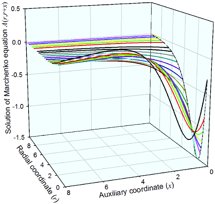
Figure 8: 3D depiction of a solution to Eq. (2) (see the explanations in the text).

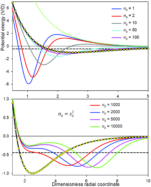
Figure 9: A family of phase-equivalent isospectral potentials calculated according to Eqs. (2)-(6). The black solid line shows the initial Morse potential, yellow circles correspond to the exact theoretical norming constant $s_{0}^{2}=y_{0}^{2}\alpha=168.18975,$ black dashed line indicates the position of the energy level $E_{0}=-\gamma_{0}^{2}=4/9,$ and green dotted line demonstrates the result of ’removing’ this level ($s_{0}=0$).

Eq. (37) has been solved using the Nyström method (see, e.g., Ref. NumRec, , p. 782), which is perfectly suitable for our purposes. As the asymptotic behavior of the kernel is known, a good idea is to split the integral into two parts and discretize them differently. Namely, for $I_{1}\equiv\int\limits_{0}^{R}F(y)dy$ the 64-point Gauss-Legendre quadrature formula can be successfully used. More specifically, the family of isospectral potentials in Fig. 9 has been calculated with $R=15,$ and splitting the range $\left[0,R\right]$ into two subdomains, so that there are 128 nodes within this region.

To discretize the asymptotic integral $I_{2}\equiv\int\limits_{R}^{\infty}F(y)dy,$ a useful trick is to change the variable Delves : $y=R+\alpha_{0}(1-u)/(1+u),$ where $\alpha_{0}>0$ is an arbitrary constant. Correspondingly, the domain of integration reduces to $\left[-1,1\right],$ where one can again use the 64-point Gauss-Legendre quadrature formula. Thus

$$I_{2}=2\alpha_{0}\int\limits_{-1}^{1}\frac{F(u)}{\left(u+1\right)^{2}}du=\sum\limits_{i}w_{i}^{\prime}F(x_{i}^{\prime}),$$ (38)

where $x_{i}^{\prime}\equiv R+\alpha_{0}(1-x_{i})/(1+x_{i}),$ $w_{i}^{\prime}\equiv 2\alpha_{0}w_{i}/\left(x_{i}+1\right)^{2}$, and $x_{i},w_{i}$ are the nodes and weights of the Gauss-Legendre formula, respectively.

The computational procedure itself is simple. Namely, using the discretized version of Eq. (37) at the specified node points $x_{n}$, one gets a system of linear algebraic equations for the quantities $T_{n}\equiv T(x_{n})$. Such a system can be easily solved. In this paper, the Householder reduction algorithm Householder was used for this purpose, because it is numerically more stable than Gaussian elimination. Having found the solution, one uses Eq. (37) once again, taking $x=0$ to get $T(0)=A(r,r).$ Finally, one calculates the potential according to Eq. (6).

The results of solving the Marchenko equation are shown in Figs. 8 and 9. The curves there were calculated with $\alpha_{0}=\Delta\cdot(1+x_{0})/(1-x_{0})$ and $\Delta=10000$ (this parameter characterizes the width of the domain). As can be seen, discretization of Marchenko equation with only 192 nodes related to the relevant quadrature formulas is sufficient to accurately solve the inverse problem. In addition, one can convince himself/herself that the sign of the second term in Eq. (3) is indeed ’minus’, while $s_{0}^{2}=y_{0}^{2}\alpha=6\exp(10/3)$, as expected.

Fig. 8 demonstrates the dependence of the solution $A(r,r+x)$ on both arguments, $r$ and $x$. In this case, the exact theoretical value for the norming constant ($s_{0}^{2}=y_{0}^{2}\alpha$) was used to fix the kernel. Actually, to calculate the potential according to Eq. (6), one only needs the solution at $x=0,$ which is shown as a background contour (dash-dot line).

In Fig. 9, a family of isospectral potentials can be seen. It was obtained by varying the norming constant $s_{0}$ in a wide range (from 0 to 100), while the scattering part of the kernel remains exactly the same for all these curves. Looking at Fig. 9, one can imagine that if the real norming constant is not known, a criterion of ’reasonableness’ could be used to fix it. For example, assuming that the potential has only one extremum point (minimum) and only one inflection point (as the Morse potential), the correct norming constant can be determined with reasonable accuracy.

VI Conclusion

In this paper, a detailed description of the full solution procedure of the Marchenko integral equation was given. To this end, the complete set of the necessary input data was used, which was obtained by accurately solving the direct Schrödinger problem for a model system. Such a tautological combination of the direct and inverse scattering problems may seem useless for practical purposes, but one has to bear in mind that otherwise the full set of necessary data cannot be obtained at all. Unfortunately, the methods of the inverse scattering theory are still not implemented as planned. These methods have mainly been used to construct families of isospectral potentials AM ; Pursey , and they have many interesting applications in the soliton theory (see, e.g., EvH ; Ablowitz ), but their capabilities have not been fully exploited. Hopefully, the results of this work clearly demonstrate the real power of the Marchenko method, albeit the necessary input data were obtained computationally, not experimentally. On the other hand, the model system used for this purpose, the well-known Morse potential, continues to surprise us by its undiscovered analytical properties. For example, in this paper a simple formula for calculating the phase shift was derived, along with the new analytic algorithm for calculating the Riemann-Siegel function, which is a pure mathematical result.

How could the results of this work be useful for further studies? An interesting option is to combine Eq. (2) with the Marchenko differential equation (see, e.g., Ref. Chadan, , p. 78), assuming that the real potential can be expressed as a sum $V(r)=V_{0}(r)+\Delta V$, where $V_{0}(r)$ is a known model potential whose spectral characteristics are known as well. Thus according to Eq. (6), $V_{0}(r)=-2\left[A_{0}(r,r)\right]^{\prime},$ where $A_{0}(r,t)$ is the corresponding solution to Eq. (2). Then, assuming that $V(r)=-2\left[A(r,r)\right]^{\prime}$ and $A(r,t)=A_{0}(r,t)+\Delta A$, one gets an equation

$$\left(\frac{\partial^{2}}{\partial r^{2}}-\frac{\partial^{2}}{\partial t^{2}}\right)\Delta A(r,t)=V_{0}(r)\Delta A(r,t)+\Delta V(r)A_{0}(r,t).$$ (39)

If $V_{0}(r)$ is sufficiently close to the real potential, the right side of Eq. (39) would contain two small quantities, $\Delta V$ and $\Delta A$, which, in principle, can be determined self-consistently along with solving this equation.

References

- (1) N. Levinson, K. Danske Vidensk. Selsk. Mat-fys. Medd. 25, 9 (1949).
- (2) N. Levinson, Mat. Tidsskr. B 13, 25 (1949).
- (3) V. Bargmann, Phys. Rev. 75, 301 (1949).
- (4) V. Bargmann, Rev. Mod. Phys. 21, 488 (1949).
- (5) I. M. Gel’fand and B. M. Levitan, Izv. Akad. Nauk SSSR. Ser. Mat. 15, 309 (1951) [Am. Math. Soc. Transl. (ser. 2) 1, 253 (1955)].
- (6) R. Jost and W. Kohn, Phys. Rev. 87, 977 (1952).
- (7) R. Jost and W. Kohn, Phys. Rev. 88, 382 (1952).
- (8) V. A. Marchenko, Dokl. Akad. Nauk SSSR 72, 457 (1950).
- (9) V. A. Marchenko, Dokl. Akad. Nauk SSSR 104, 695 (1955).
- (10) M. G. Krein, Dokl. Akad. Nauk SSSR 76, 21 (1951).
- (11) M. G. Krein, Dokl. Akad. Nauk SSSR 111, 1167 (1956).
- (12) K. Chadan and P. C. Sabatier, Inverse Problems in Quantum Scattering Theory (2nd edn.), Springer, New York, 1989.
- (13) R. Hellmann, E. Bich, and E. Vogel, Mol. Phys. 106, 133 (2008).
- (14) P. M. Morse, Phys. Rev. 34, 57 (1929).
- (15) A. Wüest and F. Merkt, J. Chem. Phys. 118, 8807 (2003).
- (16) L. Gendenshtein, Pis’ma v ZETF 38, 299 (1983).
- (17) M. Selg, Phys. Rev. E 64, 056701 (2001).
- (18) M. Selg, J. Chem. Phys. 136, 114113 (2012).
- (19) H. M. Edwards, Riemann’s Zeta Function, Academic Press, New York, 1974, Chapter 7.
- (20) K. Chadan and P. C. Sabatier, Inverse Problems in Quantum Scattering Theory, Springer, New York, 1977.
- (21) R. Pike and P. Sabatier (Eds.), Scattering and Inverse Scattering in Pure and Applied Science, Academic Press, San Diego, 2002.
- (22) K. Chadan, D. Coltort, L. Päivarinta, and W. Rundell, An Introduction to Inverse Scattering and Inverse Spectral Problems, SIAM, Philadelphia, 1997.
- (23) Z. S. Agranovitz and V. A. Marchenko, The Inverse Problem of Scattering Theory, Gordon and Breach, New York, 1963.
- (24) V. A. Marchenko, Sturm-Liouville Operators and Applications, Birkhäuser, Basel, 1986.
- (25) M. Selg, Mol. Phys. 104, 2671 (2006).
- (26) V. Chebotarev, Am. J. Phys. 66, 1086 (1998).
- (27) H. Bateman and A. Erdélyi. Higher Transcendental Functions. Vol. 1, Mc Graw-Hill, New York (1953).
- (28) M. Selg, J. Mol. Spectrosc. 220, 187 (2003).
- (29) M. Abramowitz and I. A. Stegun, Handbook of Mathematical Functions (10th printing), Dover, New York, 1972.
- (30) W. H. Press, S. A. Teukolsky, W. T. Vetterling, and B. P. Flannery, Numerical Recipes in Fortran 77, The Art of Scientific Computing (2nd edn.), Vol. 1, Cambridge University Press (1997).
- (31) L. M. Delves and J. L. Mohamed, Computational Methods for Integral Equations, Cambridge University Press, Cambridge, 1985, p. 43.
- (32) A. S. Householder, J. ACM 5, 339 (1958).
- (33) P. B. Abraham and H. E. Moses, Phys. Rev. A 22, 1333 (1980).
- (34) D. L. Pursey, Phys. Rev. D 33, 1048 (1986).
- (35) W. Eckhaus and A. van Harten, The Inverse Scattering Transformation and The Theory of Solitons, North-Holland, Amsterdam, 1981.
- (36) M. J. Ablowitz and P. A. Clarkson, Solitons, Nonlinear Evolution Equations and Inverse Scattering, Cambridge University Press, 1991.