An improved algorithm for reconstructing reflectionless potentials

Abstract

A fully algebraic approach to reconstructing one-dimensional reflectionless potentials is described. A simple and easily applicable general formula is derived, using the methods of the theory of determinants. In particular, useful properties of special determinants – the alternants – have been exploited. The main formula takes an especially simple form if one aims to reconstruct a symmetric reflectionless potential. Several examples are presented to illustrate the efficiency of the method.

I Introduction

Formulation and solution of inverse problems is an increasingly important field of scientific research. However, compared with a well-posed (in Hadamard’s sense) direct or forward problem, the corresponding inverse problem is much more difficult and, as a rule, ill-posed. Inverse scattering problem can be considered an exception to this rule. Namely, in the simplest one-dimensional case, the inverse scattering theory provides strict mathematical criteria for the existence, uniqueness and stability of the solution. It means that in this particular case the inverse problem is well-posed as well.

The related forward problem is the solution of the simplest time-independent Schrödinger equation

$$\Psi^{\prime\prime}(x)=\frac{V(x)-E}{C}\Psi(x),~{}C\equiv\frac{\hbar^{2}}{2m}$$ (1)

for a given potential $V(x)$, and subjected to appropriate physical boundary conditions. Eq. (1) can be easily solved numerically and thus, in principle, all spectral characteristics of the potential $V(x)$ can be accurately ascertained.

The inverse problem is to determine the unknown potential starting from the known spectral characteristics. This is a serious task even in this simple case for the following reasons:

• It is not obvious what kind of input information is actually needed to solve the problem uniquely.

• There must be a theoretical basis (a fundamental equation) which enables to solve the problem.

• Apart from the theoretical difficulties, another important question arises: how to obtain the necessary input data?

• Even if the mentioned principal barriers could be overcome, the computational-technical solution of the problem is not at all trivial.

Issues 1 and 2 have been successfully resolved in early 1950s for the class of potentials on the half line: $x\in\left[0,\infty\right)$. The necessary and sufficient conditions for the unique solution of the inverse problem have been formulated in a series of outstanding theoretical works by Marchenko Marchenko1 ; Marchenko2 , Gelfand, Levitan GL , Krein Krein1 ; Krein2 and others (see, e.g., CS , section III.7 for a brief overview). In addition, three different methods to solve the problem have been worked out, based on the integral equations by Gelfand-Levitan GL , Marchenko Marchenko2 and Krein Krein2 .

Solution of the inverse scattering problem on the full line ($-\infty<x<\infty$) is a more challenging problem, which was first addressed by Kay Kay , Moses Moses , and few years later in a series of papers by Faddeev Faddeev58 ; Faddeev59 ; Faddeev64 ; Faddeev74 . These fundamental studies provide full description of the solution procedure, while the correct necessary and sufficient criteria for the uniqueness of the solution were given by Marchenko (see MarchenkoBook , section III.5). These criteria apply to the following pair of integral equations Moses ; Faddeev74 ; MarchenkoBook :

$$K_{1}(x,y)+A_{1}(x+y)+\int\limits_{x}^{\infty}A_{1}(z+y)K_{1}(x,z)dz=0,$$ (2)

$$K_{2}(x,y)+A_{2}(x+y)+\int\limits_{-\infty}^{x}A_{2}(z+y)K_{2}(x,z)dz=0,$$ (3)

which are formally very similar to the Marchenko equation on the half line (see MarchenkoBook , p. 218). On the other hand, their operator-theoretical content is closer to the Gelfand-Levitan approach. Therefore, as a kind of compromise, Eqs. (2)-(3) are often called Gelfand-Levitan-Marchenko (GLM) equations. The kernel $A_{1}$ in Eq. (2) (where $y>x$) is completely specified by the so-called right scattering data, while the kernel $A_{2}$ in Eq. (3) ($y<x$) is determined by the left scattering data. These two sets of input data are equivalent: the left data are uniquely determined by the right ones and vice versa. In the following analysis we will rely on Eq. (2). If one is able to solve this integral equation then the potential is given by

$$V(x)=-2C\frac{dK_{1}(x,x)}{dx}.$$ (4)

Now, let us briefly discuss Point 3 in the above list. Unfortunately, the criteria for the uniqueness of the solution are so strict that it is nearly impossible to get all the necessary input data experimentally. However, if one sets an additional constraint that the resulting potential must be reflectionless then the inverse scattering problem can be solved much more easily. Moreover, a symmetric reflectionless potential is uniquely determined if its full spectrum of bound states is known. In the following analysis it is assumed that the potential $V(x)$ that corresponds to Eq. (4) is reflectionless by definition.

As the general principles of building confining reflectionless potentials are long known Faddeev74 ; Thacker , a natural question arises: is there any need to revisit the topic? A motivation comes from Point 4 stated above: if the total number of bound states is large then the technical side of the procedure becomes important. This in turn motivates development of more efficient algorithms. In this paper, a new analytic algorithm is derived, which enables to easily calculate a reflectionless potential with an arbitrary number ($N$) of bound states.

The paper is organized as follows. In Sec. II, the general principles are briefly described, which form the overall basis for the approach.  Secs. III and IV make an excursion to the theory of determinants, the benefits of which are described and illustrated in Sec. V. Finally, Sec. VI concludes the work.

II Reconstruction of reflectionlesss potentials: universal recipe

Suppose we are given $2N$ parameters for an unknown reflectionless potential $V(x)$: the positions of $N$ discrete energy levels $E_{n}=-C\kappa_{n}^{2}$ and $N$ norming constants$\ C_{n}$ ($n=1,2,...,N$) for the Jost solution $\Psi_{1}(i\kappa_{n},x)\$of Eq. (1), so that $\Psi_{1}(i\kappa_{n},x)\rightarrow\exp(-\kappa_{n}x)$ as $x\rightarrow+\infty,$ and

$$\int\limits_{-\infty}^{\infty}\Psi_{n}^{2}(x)dx=1,\text{ }\Psi_{n}\equiv C_{n}\Psi_{1}(i\kappa_{n},x).$$ (5)

Then it can be shown Thacker that

$$\Psi_{n}(x)=-\dfrac{1}{\Lambda_{n}(x)}\dfrac{\det\left[A^{(n)}\right]}{\det\left(A\right)}.$$ (6)

Here $A$ is a symmetric matrix with the following elements:

$$A_{mn}=\delta_{mn}+\dfrac{\Lambda_{m}(x)\Lambda_{n}(x)}{\kappa_{m}+\kappa_{n}},$$ (7)

$A^{(n)}$ is obtained from $A$ by replacing the $n$th column with its derivative, and

$$\Lambda_{n}(x)\equiv C_{n}\exp(-\kappa_{n}\,x).$$ (8)

A simple formula can also be obtained for the potential Faddeev74 ; Thacker :

$$V(x)=-2C\dfrac{d^{2}}{dx^{2}}\left\{\ln\left[\det(A)\right]\right\},$$ (9)

which is uniquely determined by parameters $\kappa_{n}$ and $C_{n}.$

Note that the potential remains unchanged if $\det\left(A\right)$ is multiplied by a function $\exp\left(\alpha x+\beta\right)$, where $\alpha$ and $\beta$ are arbitrary constants. Consequently, we can multiply, for example, any row of the initial matrix by a function $\exp\left[\kappa_{n}(x-x_{n})\right]$ ($n=1,2,...,N$), where $x_{n}$ are new parameters, equivalent to norming constants:

$$\exp\left(2\kappa_{n}x_{n}\right)\equiv\dfrac{C_{n}^{2}}{2\kappa_{n}},$$ (10)

and thus, according to definition (8),

$$\dfrac{\Lambda_{n}^{2}(x)}{2\kappa_{n}}=\exp\left[-2\kappa_{n}(x-x_{n})\right].$$ (11)

As a result, we get another matrix which contains full information for reconstructing the potential according to Eq. (9):

$$\begin{array}[]{c}\tilde{A}_{N}=\tilde{B}_{N}+\tilde{C}_{N},\\ V(x)=-2C\dfrac{d^{2}}{dx^{2}}\left\{\ln\left[\det(\tilde{A}_{N})\right]\right\}.\end{array}$$ (12)

Here

$$\tilde{B}_{N}\equiv\left(\begin{array}[]{cccc}e^{\kappa_{1}(x-x_{1})}&0&...&0\\ 0&e^{\kappa_{2}(x-x_{2})}&...&0\\ 0&...&...&...\\ 0&...&...&e^{\kappa_{N}(x-x_{N})}\end{array}\right)$$ (13)

and

$$\tilde{C}_{N}\equiv\left(\begin{array}[]{cccc}e^{-\kappa_{1}(x-x_{1})}&\frac{2\sqrt{\kappa_{1}\kappa_{2}}}{\kappa_{1}+\kappa_{2}}e^{-\kappa_{2}(x-x_{2})}&...&\frac{2\sqrt{\kappa_{1}\kappa_{N}}}{\kappa_{1}+\kappa_{N}}e^{-\kappa_{n}(x-x_{N})}\\ \frac{2\sqrt{\kappa_{1}\kappa_{2}}}{\kappa_{1}+\kappa_{2}}e^{-\kappa_{1}(x-x_{1})}&e^{-\kappa_{2}(x-x_{2})}&...&\frac{2\sqrt{\kappa_{2}\kappa_{N}}}{\kappa_{2}+\kappa_{N}}e^{-\kappa_{n}(x-x_{N})}\\ ...&...&...&...\\ \frac{2\sqrt{\kappa_{1}\kappa_{N}}}{\kappa_{1}+\kappa_{N}}e^{-\kappa_{1}(x-x_{1})}&\frac{2\sqrt{\kappa_{2}\kappa_{N}}}{\kappa_{2}+\kappa_{N}}e^{-\kappa_{2}(x-x_{2})}&...&e^{-\kappa_{N}(x-x_{N})}\end{array}\right).$$ (14)

Remark: A subscript was added to denote the number of the bound states (and the rank of the matrix).

From now on, the determinants having the structure $\det(A)\cdot\exp\left(\alpha x+\beta\right)$ with the elements $A_{mn}$ defined in Eq. (7), will be sometimes called $\tau$-functions (as is common in soliton theory). In the next two sections it will be shown that such determinants can be easily calculated even for an arbitrarily large $N$.

III General formula for the $\tau$-functions

To evaluate a non-trivial determinant, one can use the Laplace expansion (see Meyer , p. 487) in terms of the fixed row (or column) indices. For example, choosing a set of indices $m_{1},$ $m_{2},...,m_{k}$ for an arbitrary $N\times N$-matrix $A_{N}$, so that $1\leq m_{1}<m_{2}<...\leq N$, we get

$$\det\left(A_{N}\right)=\sum\limits_{1\leq n_{1}<n_{2}<...\leq N}\det A\left(m_{1}m_{2}...m_{k}\right|n_{1}n_{2}...n_{k})\times$$ (15)

$$\det\widehat{A}\left(m_{1}m_{2}...m_{k}\right|n_{1}n_{2}...n_{k}).$$

Here $A\left(m_{1}m_{2}...m_{k}\right|n_{1}n_{2}...n_{k})$ is a $k\times k$-submatrix of $A_{N}$ that lies on the intersection of rows $m_{1},$ $m_{2},...,m_{k}$ and columns $n_{1},$ $n_{2},...,n_{k}$, while

$$\det\widehat{A}\left(m_{1}m_{2}...m_{k}\right|n_{1}n_{2}...n_{k})=$$

$$(-1)^{m_{1}+...+m_{k}+n_{1}...+n_{k}}M\left(m_{1}m_{2}...m_{k}\right|n_{1}n_{2}...n_{k}),$$

and $M\left(m_{1}m_{2}...m_{k}\right|n_{1}n_{2}...n_{k})$ is a minor obtained from $\det\left(A_{N}\right)$ by deleting rows $m_{1},$ $m_{2},...,m_{k}$ and columns $n_{1},$ $n_{2},...,n_{k}$.

Consequently, applying Eq. (15) to the $\tau$-function defined by Eqs. (12)-(14),

$$\tau_{N}\equiv\det\left(\tilde{A}_{N}\right)=a_{0}\exp(\alpha_{0})+\sum_{i=1}^{N}a_{i}\exp(\alpha_{i})+$$ (16)

$$\sum_{1\leq i<j\leq N}a_{ij}\exp(\alpha_{ij})+\sum\limits_{1\leq i<j<k\leq N}a_{ijk}\exp(\alpha_{ijk})+$$

$$...+a_{123...N}\exp(\alpha_{123...N}),$$

where the coefficients $a_{0},$ $a_{i},$ $a_{ij},$ $a_{ijk}$,… as well as the corresponding arguments of the exponents can be easily fixed with the help of Eqs. (12)-(14). Indeed,

$$\alpha_{0}=\sum_{l=1}^{N}\kappa_{l}(x-x_{l}),\ \alpha_{i}=\sum_{l=1}^{N}(-1)^{\delta_{il}}\kappa_{l}(x-x_{l}),$$ (17)

$$\alpha_{ij}=\sum_{m=1}^{N}(-1)^{\delta_{im}+\delta_{jm}}\kappa_{m}(x-x_{m}),$$

$$\alpha_{ijk}=\sum\limits_{n=1}^{N}(-1)^{\delta_{in}+\delta_{jn}+\delta_{kn}}\kappa_{n}(x-x_{n}),$$

$$...\alpha_{123...N}=\sum\limits_{n=1}^{N}(-1)^{\delta_{1n}+\delta_{2n}+...\delta_{Nn}}\kappa_{n}(x-x_{n})=-\alpha_{0},$$

$\delta_{il}$ being the Kronecker’s symbol.

To further simplify Eq. (16), let us group the terms into pairs, so that the arguments of the corresponding exponents differ only by sign. For example, the first pair is formed of the terms with coefficients

$$a_{0}=1$$

and

$$a_{123...N}\equiv A_{0}^{2}=$$

$$\left|\begin{array}[]{cccc}1&\frac{2\sqrt{\kappa_{1}\kappa_{2}}}{\kappa_{1}+\kappa_{2}}&...&\frac{2\sqrt{\kappa_{1}\kappa_{N}}}{\kappa_{1}+\kappa_{N}}\\ \frac{2\sqrt{\kappa_{1}\kappa_{2}}}{\kappa_{1}+\kappa_{2}}&1&...&\frac{2\sqrt{\kappa_{2}\kappa_{N}}}{\kappa_{2}+\kappa_{N}}\\ ...&...&...&...\\ \frac{2\sqrt{\kappa_{1}\kappa_{N}}}{\kappa_{1}+\kappa_{N}}&\frac{2\sqrt{\kappa_{2}\kappa_{N}}}{\kappa_{2}+\kappa_{N}}&...&1\end{array}\right|.$$

Note that

$$\det\left(\tilde{B}_{N}\right)=a_{0}\exp(\alpha_{0}),\ \det\left(\tilde{C}_{N}\right)=a_{123...N}\exp(-\alpha_{0}).$$

Here we defined a new coefficient $A_{0}$, whose subscript ”0” emphasizes that the expression $-\alpha_{0}=-\kappa_{1}(x-x_{1})-\kappa_{2}(x-x_{2})-...-\kappa_{N}(x-x_{N})$ contains no terms (0 terms) with plus sign. The same logic can be applied to all terms of Eq. (16). For example, the appropriate partner for the term $a_{1}\exp(\alpha_{1})$ is $a_{234...N}\exp(-\alpha_{1}),$ where

$$a_{1}=1,$$

$$a_{234...N}\equiv A_{1}^{2}=$$

$$\left|\begin{array}[]{cccc}1&\frac{2\sqrt{\kappa_{2}\kappa_{3}}}{\kappa_{2}+\kappa_{3}}&...&\frac{2\sqrt{\kappa_{2}\kappa_{N}}}{\kappa_{2}+\kappa_{N}}\\ \frac{2\sqrt{\kappa_{2}\kappa_{3}}}{\kappa_{2}+\kappa_{3}}&1&...&\frac{2\sqrt{\kappa_{3}\kappa_{N}}}{\kappa_{3}+\kappa_{N}}\\ ...&...&...&...\\ \frac{2\sqrt{\kappa_{2}\kappa_{N}}}{\kappa_{2}+\kappa_{N}}&\frac{2\sqrt{\kappa_{3}\kappa_{N}}}{\kappa_{3}+\kappa_{N}}&...&1\end{array}\right|.$$

Analogously, we can form a pair from $a_{12}\exp(\alpha_{12})$ and $a_{345...N}\exp(-\alpha_{12})$, where

$$a_{12}=\left|\begin{array}[]{cc}1&\frac{2\sqrt{\kappa_{1}\kappa_{2}}}{\kappa_{1}+\kappa_{2}}\\ \frac{2\sqrt{\kappa_{1}\kappa_{2}}}{\kappa_{1}+\kappa_{2}}&1\end{array}\right|,$$

$$a_{345...N}=\left|\begin{array}[]{cccc}1&\frac{2\sqrt{\kappa_{3}\kappa_{4}}}{\kappa_{3}+\kappa_{4}}&...&\frac{2\sqrt{\kappa_{3}\kappa_{N}}}{\kappa_{3}+\kappa_{N}}\\ \frac{2\sqrt{\kappa_{3}\kappa_{4}}}{\kappa_{3}+\kappa_{4}}&1&...&\frac{2\sqrt{\kappa_{4}\kappa_{N}}}{\kappa_{4}+\kappa_{N}}\\ ...&...&...&...\\ \frac{2\sqrt{\kappa_{3}\kappa_{N}}}{\kappa_{3}+\kappa_{N}}&\frac{2\sqrt{\kappa_{4}\kappa_{N}}}{\kappa_{4}+\kappa_{N}}&...&1\end{array}\right|.$$

The principle is simple: for any $a_{n_{1}n_{2}...n_{i}}\exp(\alpha_{n_{1}n_{2}...n_{i}})$ the partner is $a_{n_{i+1}n_{i+2}...n_{N}}\exp(-\alpha_{n_{1}n_{2}...n_{i}}).$ In addition, as we will see below, it is convenient to define a relevant coefficient

$$A_{n_{1}n_{2}...n_{i}}^{2}\equiv a_{n_{1}n_{2}...n_{i}}\cdot a_{n_{i+1}n_{i+2}...n_{N}},$$ (18)

where the indices point at the terms with plus sign on the right side of the expression

$$-\alpha_{n_{1}...n_{i}}=\kappa_{n_{1}}(x-x_{n_{1}})+...$$ (19)

$$+\kappa_{n_{i}}(x-x_{n_{i}})-\kappa_{n_{i+1}}(x-x_{n_{i+1}})-...$$

Looking at the structure of the matrix $\tilde{A}_{N}$, it is obvious that all these plus sign terms can only originate from the expansion of $\det\left(\tilde{B}_{N}\right)$ and they correspond to the product $(\tilde{B}_{N})_{n_{1}n_{1}}\cdot(\tilde{B}_{N})_{n_{2}n_{2}}\cdot...\cdot(\tilde{B}_{N})_{n_{i}n_{i}}.$ The terms with minus sign on the right side of Eq. (19) are related to the expansion of $\det\left(\tilde{C}_{N}\right),$ without any contribution from $\det\left(\tilde{B}_{N}\right).$

On the basis of the above arguments, the following conclusions can be made:

• All terms on the right side of Eq. (16) can be grouped into pairs. There is only one term, $a_{123...N}\exp(-\alpha_{0})=\det\left(\tilde{C}_{N}\right)$ (with partner $\det\left(\tilde{B}_{N}\right)=a_{0}\exp(\alpha_{0})$) which is entirely formed of the elements of the matrix $\tilde{C}_{N}$. Any other term (both partners) contains some diagonal elements of the matrix $\tilde{B}_{N}$ as well.

• Any term $a_{n_{1}n_{2}...n_{i}}\exp(\alpha_{n_{1}n_{2}...n_{i}})$ ($i=1,2,...$) can be obtained by replacing all elements of the rows and columns $n_{i+1},n_{i+2},...n_{N}$ of the matrix $\tilde{C}_{N}$ with corresponding elements of the matrix $\tilde{B}_{N}$ (mostly with zeros). As a result, one gets a modified matrix $\widehat{C}_{N}$, while $a_{n_{1}n_{2}...n_{i}}\exp(\alpha_{n_{1}n_{2}...n_{i}})=\det\left(\widehat{C}_{N}\right).$ The Laplace expansion (15) of this determinant for the fixed rows $n_{i+1},n_{i+2},...n_{N}$ contains only one term!

• For any term $a_{n_{1}n_{2}...n_{i}}\exp(\alpha_{n_{1}n_{2}...n_{i}})$ of the expansion (16) there is a partner

  $$a_{n_{i+1}n_{i+2}...n_{N}}\exp(-\alpha_{n_{1}n_{2}...n_{i}})=\det\left(\overline{C}_{N}\right),$$

  where $\overline{C}_{N}$ can be obtained by replacing all elements of the rows and columns $n_{1},n_{2},...n_{i}$ of the matrix $\tilde{C}_{N}$ with corresponding elements of the matrix $\tilde{B}_{N}$. The Laplace expansion of $\det\left(\overline{C}_{N}\right)$ for the rows $n_{1},n_{2},...n_{i}$ also contains only one term:

  $$\det\left(\overline{C}_{N}\right)=\exp(-\alpha_{12...i})\times$$ (20)

  $$\left|\begin{array}[]{cccc}1&\frac{2\sqrt{\kappa_{n_{i+1}}\kappa_{n_{i+2}}}}{\kappa_{n_{i+1}}+\kappa_{n_{i+2}}}&...&\frac{2\sqrt{\kappa_{n_{i+1}}\kappa_{n_{N}}}}{\kappa_{n_{i+1}+}\kappa_{n_{N}}}\\ \frac{2\sqrt{\kappa_{n_{i+1}}\kappa_{n_{i+2}}}}{\kappa_{n_{i+1}}+\kappa_{n_{i+2}}}&1&...&\frac{2\sqrt{\kappa_{n_{i+2}}\kappa_{n_{N}}}}{\kappa_{n_{i+2}+}\kappa_{n_{N}}}\\ ...&...&...&...\\ \frac{2\sqrt{\kappa_{n_{i+1}}\kappa_{n_{N}}}}{\kappa_{n_{i+1}+}\kappa_{n_{N}}}&\frac{2\sqrt{\kappa_{n_{i+2}}\kappa_{n_{N}}}}{\kappa_{n_{i+2}+}\kappa_{n_{N}}}&...&1\end{array}\right|.$$ (25)

  It means, for example, that

  $$A_{12...i}^{2}=a_{12...i}\cdot a_{i+1,i+2,...N}=$$ (26)

  $$\left|\begin{array}[]{cccc}1&\frac{2\sqrt{\kappa_{1}\kappa_{2}}}{\kappa_{1}+\kappa_{2}}&...&\frac{2\sqrt{\kappa_{1}\kappa_{i}}}{\kappa_{1}+\kappa_{i}}\\ \frac{2\sqrt{\kappa_{1}\kappa_{2}}}{\kappa_{1}+\kappa_{2}}&1&...&\frac{2\sqrt{\kappa_{2}\kappa_{i}}}{\kappa_{2}+\kappa_{i}}\\ ...&...&...&...\\ \frac{2\sqrt{\kappa_{1}\kappa_{i}}}{\kappa_{1}+\kappa_{i}}&\frac{2\sqrt{\kappa_{2}\kappa_{i}}}{\kappa_{2}+\kappa_{i}}&...&1\end{array}\right|\times$$ (31)

  $$\left|\begin{array}[]{cccc}1&\frac{2\sqrt{\kappa_{i+1}\kappa_{i+2}}}{\kappa_{i+1}+\kappa_{i+2}}&...&\frac{2\sqrt{\kappa_{i+1}\kappa_{N}}}{\kappa_{i+1}+\kappa_{N}}\\ \frac{2\sqrt{\kappa_{i+1}\kappa_{i+2}}}{\kappa_{i+1}+\kappa_{i+2}}&1&...&\frac{2\sqrt{\kappa_{n_{i+2}}\kappa_{n_{N}}}}{\kappa_{n_{i+2}+}\kappa_{n_{N}}}\\ ...&...&...&...\\ \frac{2\sqrt{\kappa_{i+1}\kappa_{N}}}{\kappa_{i+1}+\kappa_{N}}&\frac{2\sqrt{\kappa_{n_{i+2}}\kappa_{n_{N}}}}{\kappa_{n_{i+2}+}\kappa_{n_{N}}}&...&1\end{array}\right|.$$ (36)

• One should avoid re-use of the terms: an already existing pair must not be included again! It means that the members of the modified expansion (16) are identified by no more than $\left[N/2\right]$ indices (square brackets denote integer part of $N/2$). It is convenient to group the members on the basis of the number of indices, so that there will be $0,1,2,...,$ $\left[N/2\right]$ different indices.

As the final result of the above analysis, we get the following general formula:

$$\tau_{N}=\det\left(\tilde{A}_{N}\right)=\sum\limits_{i=0}^{N}A_{i}\left[\exp(\alpha_{i}+\beta_{i})+\exp(-\alpha_{i}-\beta_{i})\right]+$$

$$...+\sum\limits_{1\leq i_{1}<...<i_{\left[N/2\right]}\leq N}A_{i_{1}...i_{\left[N/2\right]}}[\exp(\alpha_{i_{1}...i_{\left[N/2\right]}}+\beta_{i_{1}...i_{\left[N/2\right]}})+$$

$$\exp(-\alpha_{i_{1}..i_{\left[N/2\right]}}-\beta_{i_{1}...i_{\left[N/2\right]}})]=\sum\limits_{i=0}^{N}2A_{i}\cosh(\alpha_{i}+\beta_{i})+$$

$$\sum\limits_{1\leq i_{1}<i_{2}\leq N}2A_{i_{1}i_{2}}\cosh(\alpha_{i_{1}i_{2}}+\beta_{i_{1}i_{2}})+...+$$ (37)

$$\sum\limits_{1\leq i_{1}<...<i_{\left[N/2\right]}\leq N}2A_{i_{1}i_{2}...i_{\left[N/2\right]}}\cosh(\alpha_{i_{1}i_{2}...i_{\left[N/2\right]}}+\beta_{i_{1}i_{2}...i_{\left[N/2\right]}}),$$

where

$$\exp(\beta_{n_{1}n_{2}...n_{i}})\equiv\dfrac{a_{n_{1}n_{2}...n_{i}}}{a_{n_{i+1}n_{i+2}...n_{N}}}.$$ (38)

It is easy to be convinced that the expansion (37) contains $2^{N-1}$ members in total (apart from inessential factor $2$). Indeed, according to Newton’s binomial theorem

$$\begin{pmatrix}N\\ 0\end{pmatrix}+\begin{pmatrix}N\\ 1\end{pmatrix}+\begin{pmatrix}N\\ 2\end{pmatrix}+\begin{pmatrix}N\\ 3\end{pmatrix}+...+=\frac{\left(1+1\right)^{N}}{2}=2^{N-1},$$

where we took into consideration that only half of this formal series is actually needed.

IV Alternants of $\tau$-functions

We have shown that not only $\det\left(\tilde{A}_{N}\right)$ itself but also the coefficients $A_{i},A_{i_{1}i_{2}},...,A_{i_{1}i_{2}...i_{\left[N/2\right]}}$ in the expansion (37) are $\tau$-functions. Consequently, the solution of the inverse scattering problem has been reduced to evaluating a number of determinants

$$D(\kappa_{1},\kappa_{2},..,\kappa_{n})\equiv\left|\begin{array}[]{cccc}1&\frac{2\sqrt{\kappa_{1}\kappa_{2}}}{\kappa_{1}+\kappa_{2}}&...&\frac{2\sqrt{\kappa_{1}\kappa_{n}}}{\kappa_{1}+\kappa_{n}}\\ \frac{2\sqrt{\kappa_{1}\kappa_{2}}}{\kappa_{1}+\kappa_{2}}&1&...&\frac{2\sqrt{\kappa_{2}\kappa_{n}}}{\kappa_{2}+\kappa_{n}}\\ ...&...&...&...\\ \frac{2\sqrt{\kappa_{1}\kappa_{n}}}{\kappa_{1}+\kappa_{n}}&\frac{2\sqrt{\kappa_{2}\kappa_{n}}}{\kappa_{2}+\kappa_{n}}&...&1\end{array}\right|,$$ (39)

fixed by the parameters $\kappa_{1}<\kappa_{2}<$ $...<\kappa_{n}$, $n$ being an appropriate natural number. We are now going to derive a simple formula for calculating such $\tau$-functions. First, let us set a one-to-one correspondence between each row of the determinant and a fixed parameter

$$q_{i}=\sqrt{\kappa_{i}}\ \left(i=1,2,...,n\right).$$ (40)

For example, the modified elements of the first row of Eq. (39) will be

$$1=\frac{2q_{1}\sqrt{\kappa_{1}}}{q_{1}^{2}+\kappa_{1}},\text{ }\frac{2\sqrt{\kappa_{1}\kappa_{2}}}{\kappa_{1}+\kappa_{2}}=\frac{2q_{1}\sqrt{\kappa_{2}}}{q_{1}^{2}+\kappa_{2}},...,\frac{2\sqrt{\kappa_{1}\kappa_{n}}}{\kappa_{1}+\kappa_{n}}=\frac{2q_{1}\sqrt{\kappa_{n}}}{q_{1}^{2}+\kappa_{n}}.$$

The usefulness of this trick soon becomes evident, although there seems to be only a formal change:

$$D(\kappa_{1},\kappa_{2},..,\kappa_{n})\equiv\left|\begin{array}[]{cccc}\frac{2q_{1}\sqrt{\kappa_{1}}}{q_{1}^{2}+\kappa_{1}}&\frac{2q_{1}\sqrt{\kappa_{2}}}{q_{1}^{2}+\kappa_{2}}&...&\frac{2q_{1}\sqrt{\kappa_{n}}}{q_{1}^{2}+\kappa_{n}}\\ \frac{2q_{2}\sqrt{\kappa_{1}}}{q_{2}^{2}+\kappa_{1}}&\frac{2q_{2}\sqrt{\kappa_{2}}}{q_{2}^{2}+\kappa_{2}}&...&\frac{2q_{2}\sqrt{\kappa_{n}}}{q_{2}^{2}+\kappa_{n}}\\ ...&...&...&...\\ \frac{2q_{n}\sqrt{\kappa_{1}}}{q_{n}^{2}+\kappa_{1}}&\frac{2q_{n}\sqrt{\kappa_{2}}}{q_{n}^{2}+\kappa_{2}}&...&\frac{2q_{n}\sqrt{\kappa_{n}}}{q_{n}^{2}+\kappa_{n}}\end{array}\right|=$$ (45)

$$2^{n}\cdot\kappa_{1}\kappa_{2}...\kappa_{n}\left|\begin{array}[]{cccc}\frac{1}{q_{1}^{2}+\kappa_{1}}&\frac{1}{q_{1}^{2}+\kappa_{2}}&...&\frac{1}{q_{1}^{2}+\kappa_{n}}\\ \frac{1}{q_{2}^{2}+\kappa_{1}}&\frac{1}{q_{2}^{2}+\kappa_{2}}&...&\frac{1}{q_{2}^{2}+\kappa_{n}}\\ ...&...&...&...\\ \frac{1}{q_{n}^{2}+\kappa_{1}}&\frac{1}{q_{n}^{2}+\kappa_{2}}&...&\frac{1}{q_{n}^{2}+\kappa_{n}}\end{array}\right|.$$ (50)

Here we separated a factor $2q_{i}$ from each row and $\sqrt{\kappa_{i}}$ from each column, i.e., $2q_{i}\sqrt{\kappa_{i}}=2\kappa_{i}$ ($i=1,2,...,n$) from each such pair.

Next, let us transform Eq. (50) into a polynomial, multiplying each row by

$$\prod\limits_{j}\left(q_{i}^{2}+\kappa_{j}\right)\ \left(i=1,2,...,n\right).$$

The result is

$$D(\kappa_{1},\kappa_{2},..,\kappa_{n})=\dfrac{1}{\prod\limits_{1\leq i<j\leq n}\left(\kappa_{i}+\kappa_{j}\right)^{2}}\times D_{n},$$ (51)

where a new determinant

$$D_{n}\equiv\left|\begin{array}[]{cccc}\prod\limits_{j\neq 1}\left(q_{1}^{2}+\kappa_{j}\right)&\prod\limits_{j\neq 2}\left(q_{1}^{2}+\kappa_{j}\right)&...&\prod\limits_{j\neq n}\left(q_{1}^{2}+\kappa_{j}\right)\\ \prod\limits_{j\neq 1}\left(q_{2}^{2}+\kappa_{j}\right)&\prod\limits_{j\neq 2}\left(q_{2}^{2}+\kappa_{j}\right)&...&\prod\limits_{j\neq n}\left(q_{2}^{2}+\kappa_{j}\right)\\ ...&...&...&...\\ \prod\limits_{j\neq 1}\left(q_{n}^{2}+\kappa_{j}\right)&\prod\limits_{j\neq 2}\left(q_{n}^{2}+\kappa_{j}\right)&...&\prod\limits_{j\neq n}\left(q_{n}^{2}+\kappa_{j}\right)\end{array}\right|$$ (52)

was introduced. As can be seen, the factor $2^{n}\cdot\kappa_{1}\kappa_{2}...\kappa_{n}$ was canceled out from Eq. (51).

We can see that the elements of the columns of $D_{n}$ correspond to different values of the same function, while any row is characterized by a single fixed parameter. Indeed, Eq. (52) can be expressed as

$$D_{n}=\left|\begin{array}[]{cccc}F_{1}(q_{1})&F_{2}(q_{1})&...&F_{n}(q_{1})\\ F_{1}(q_{2})&F_{2}(q_{2})&...&F_{n}(q_{2})\\ ...&...&...&...\\ F_{1}(q_{n})&F_{2}(q_{n})&...&F_{n}(q_{n})\end{array}\right|,$$ (53)

where

$$F_{1}(x) \equiv \left(x^{2}+\kappa_{2}\right)\left(x^{2}+\kappa_{3}\right)...\left(x^{2}+\kappa_{n}\right),$$ (54)

$$F_{2}(x) \equiv \left(x^{2}+\kappa_{1}\right)\left(x^{2}+\kappa_{3}\right)...\left(x^{2}+\kappa_{n}\right),$$

$$F_{3}(x) \equiv \left(x^{2}+\kappa_{1}\right)\left(x^{2}+\kappa_{2}\right)\left(x^{2}+\kappa_{4}\right)...\left(x^{2}+\kappa_{n}\right),$$

$$...$$

$$F_{n}(x) \equiv \left(x^{2}+\kappa_{1}\right)\left(x^{2}+\kappa_{2}\right)\left(x^{2}+\kappa_{3}\right)...\left(x^{2}+\kappa_{n-1}\right).$$

A determinant that has a structure of Eq. (53) is called alternant (see Muir , p. 161). The best known alternant is Vandermonde’s determinant (for the same set of variables)

$$V_{n}\equiv\left|\begin{array}[]{ccccc}1&q_{1}&q_{1}^{2}&...&q_{1}^{n-1}\\ 1&q_{2}&q_{2}^{2}&...&q_{2}^{n-1}\\ ...&...&...&...&...\\ 1&q_{n-1}&q_{n-1}^{2}&...&q_{n-1}^{n-1}\\ 1&q_{n}&q_{n}^{2}&...&q_{n}^{n-1}\end{array}\right|,$$ (55)

which can be easily evaluated (see Korn , p. 16):

$$V_{n}(q_{1},q_{2},...,q_{n})=\prod\limits_{1\leq i<j\leq n}\left(q_{j}-q_{i}\right).$$ (56)

An important point is that the factor $V_{n}(q_{1},q_{2},...,q_{n})$ can be separated from any $n$th-order alternant. Indeed, the argument $q_{n}$ may only appear in the $n$th row of Eq. (53): if we put it into any other row then the determinant would be identically zero. It means that $D_{n}$ has a factor $\prod\limits_{i=1}^{n-1}\left(q_{n}-q_{i}\right).$ Analogous reasoning applied to $q_{n-1}$ shows that $D_{n}$ also has a factor $\prod\limits_{i=1}^{n-2}\left(q_{n-1}-q_{i}\right)$, etc. Putting it all together, we conclude that an $n$th-order alternate always has a factor $V_{n}(q_{1},q_{2},...,q_{n}).$

To continue the analysis, let us recall some useful properties of the elementary symmetric functions:

$$\sigma_{0} \equiv 1,$$ (57)

$$\sigma_{1} \equiv q_{1}+q_{2}+...+q_{n},$$

$$...$$

$$\sigma_{k} \equiv \sum_{1\leq i_{1}<i_{2}\cdot\cdot\cdot<i_{k}\leq n}q_{i_{1}}q_{i_{2}}\cdot\cdot\cdot\ q_{i_{k}},$$

$$...$$

$$\sigma_{n} \equiv q_{1}q_{2}\cdot\cdot\cdot\ q_{n}.$$

Here $\sigma_{k}$ ($k\geq 2$) is a sum of all possible products of exactly $k$ variables arranged in ascending order of their indices. According to the Fundamental Theorem for symmetric polynomials (see CLO , p. 312), any such polynomial can be uniquely expressed as a polynomial in $\sigma_{1},\sigma_{2},...,\sigma_{n}.$ This in turn is a basis for the following important theorem:

Theorem 1: Let $\left|A_{n}\right|$ be an $n$th order alternant generated by the functions

$$F_{j}(x) = a_{0j}+a_{1j}\cdot x+a_{2j}\cdot x^{2}+...+a_{nj}\cdot x^{n},$$ (58)

$$\ j = 1,2,...,n,$$

where the parameters $a_{ij}$ do not depend on $x$, and define

$$S_{k}\equiv\left(-1\right)^{k}\sigma_{k}(q_{1},q_{2},...,q_{n}).$$ (59)

Then

$$\dfrac{\left|A_{n}\right|}{V_{n}(q_{1},q_{2},...,q_{n})}=\left|\begin{array}[]{ccccc}a_{01}&a_{11}&a_{21}&...&a_{n1}\\ a_{02}&a_{12}&a_{22}&...&a_{n2}\\ ...&...&...&...&...\\ a_{0n}&a_{1n}&a_{2n}&...&a_{nn}\\ S_{n}&S_{n-1}&S_{n-2}&...&S_{0}\end{array}\right|\equiv\Delta_{n+1}.$$ (60)

Proof: Let us introduce an auxiliary polynomial

$$F(x)\equiv(x-q_{1})(x-q_{2})...(x-q_{n})$$ (61)

and form an $(n+1)$th order Vandermonde’s determinant, adding a new (arbitrary) variable $q_{n+1}$, so that

$$V_{n+1}(q_{1},q_{2},...,q_{n},q_{n+1})=\left|\begin{array}[]{ccccc}1&1&...&1&1\\ q_{1}&q_{2}&...&q_{n}&q_{n+1}\\ ...&...&...&...&...\\ q_{1}^{n-1}&q_{2}^{n-1}&...&q_{n}^{n-1}&q_{n+1}^{n-1}\\ q_{1}^{n}&q_{2}^{n}&...&q_{n}^{n}&q_{n+1}^{n}\end{array}\right|$$

(compared with Eq. (55), the row and column indices are interchanged). Multiplying $\Delta_{n+1}\$by $V_{n+1}$ and using Eqs. (58), (59), (61), we get

$$\Delta_{n+1}\times V_{n+1}=\left|\begin{array}[]{ccccc}F_{1}(q_{1})&F_{1}(q_{2})&...&F_{1}(q_{n})&F_{1}(q_{n+1})\\ F_{2}(q_{1})&F_{2}(q_{2})&...&F_{2}(q_{n})&F_{2}(q_{n+1})\\ ...&...&...&...&...\\ F_{n}(q_{1})&F_{n}(q_{2})&...&F_{n}(q_{n})&F_{n}(q_{n+1})\\ F(q_{1})&F(q_{2})&...&F(q_{n})&F(q_{n+1})\end{array}\right|=$$

$$\left|\begin{array}[]{ccccc}F_{1}(q_{1})&F_{1}(q_{2})&...&F_{1}(q_{n})&F_{1}(q_{n+1})\\ F_{2}(q_{1})&F_{2}(q_{2})&...&F_{2}(q_{n})&F_{2}(q_{n+1})\\ ...&...&...&...&...\\ F_{n}(q_{1})&F_{n}(q_{2})&...&F_{n}(q_{n})&F_{n}(q_{n+1})\\ 0&0&...&0&F(q_{n+1})\end{array}\right|$$

or, in a more compact form,

$$\Delta_{n+1}\times V_{n+1}=(q_{n+1}-q_{1})...(q_{n+1}-q_{n})\times\left|A_{n}\right|,$$ (62)

where we took into consideration that $F(q_{i})=0$ if $i=1,2,...,n.$

From Eq. (56) one concludes that

$$V_{n+1}=(q_{n+1}-q_{1})(q_{n+1}-q_{2})...(q_{n+1}-q_{n})\cdot V_{n},$$

so that both sides of Eq. (62) contain a common divisor $(q_{n+1}-q_{1})(q_{n+1}-q_{2})...(q_{n+1}-q_{n})\neq 0$. Consequently, $\Delta_{n+1}V_{n}=\left|A_{n}\right|,$ Q. E. D.

IV.1 Relationship to the inverse scattering problem

Let us apply Theorem 1 to the alternant (53) generated by the functions (54), which are polynomials in a variable $x^{2}$. Using Eqs. (58) and (59), one gets

$$a_{01} = \sigma_{n-1}(\kappa_{2},\kappa_{3},...,\kappa_{n}),$$

$$\ a_{11} = \sigma_{n-2}(\kappa_{2},\kappa_{3},...,\kappa_{n}),...,a_{n-1,1}=1,\ a_{n1}=0,$$

$$a_{02} = \sigma_{n-1}(\kappa_{1},\kappa_{3},...,\kappa_{n}),$$

$$\ a_{12} = \sigma_{n-2}(\kappa_{1},\kappa_{3},...,\kappa_{n}),...,a_{n-1,2}=1,\ a_{n2}=0,$$

$$...$$

$$a_{0n} = \sigma_{n-1}(\kappa_{1},\kappa_{2},...,\kappa_{n-1}),$$

$$a_{1n} = \sigma_{n-2}(\kappa_{1},\kappa_{2},...,\kappa_{n-1}),...,a_{n-1,n}=1,\ a_{nn}=0.$$

Consequently,

$$D_{n}=V_{n}(q_{1},q_{2},...,q_{n})\times\left|R_{n}\right|,~{}\left|R_{n}\right|\equiv$$ (63)

$$\left|\begin{array}[]{ccccc}\sigma_{n-1}(\kappa_{2},\kappa_{3},...,\kappa_{n})&\sigma_{n-2}(\kappa_{2},\kappa_{3},...,\kappa_{n})&...&1&0\\ \sigma_{n-1}(\kappa_{1},\kappa_{3},...,\kappa_{n})&\sigma_{n-2}(\kappa_{1},\kappa_{3},...,\kappa_{n})&...&1&0\\ ...&...&...&...&...\\ \sigma_{n-1}(\kappa_{1},\kappa_{2},...,\kappa_{n-1})&\sigma_{n-2}(\kappa_{1},\kappa_{2},...,\kappa_{n-1})&...&1&0\\ S_{n}&S_{n-1}&...&S_{1}&S_{0}\end{array}\right|=$$ (69)

$$\left|\begin{array}[]{cccc}\sigma_{n-1}(\kappa_{2},\kappa_{3},...,\kappa_{n})&\sigma_{n-2}(\kappa_{2},\kappa_{3},...,\kappa_{n})&...&1\\ \sigma_{n-1}(\kappa_{1},\kappa_{3},...,\kappa_{n})&\sigma_{n-2}(\kappa_{1},\kappa_{3},...,\kappa_{n})&...&1\\ ...&...&...&...\\ \sigma_{n-1}(\kappa_{1},\kappa_{2},...,\kappa_{n-1})&\sigma_{n-2}(\kappa_{1},\kappa_{2},...,\kappa_{n-1})&...&1\end{array}\right|.$$ (74)

Here we defined a new determinant $\left|R_{n}\right|$ which seems to be another alternant, so we can apply Theorem 1 to evaluate it. To be convinced that $\left|R_{n}\right|$ is indeed an alternant, we have to specify the generating functions. Obviously,

$$F_{n}(x) = 1=\sigma_{0}(\kappa_{1},\kappa_{2},...,\kappa_{n}),$$ (75)

$$F_{n-1}(x) = \sigma_{1}(\kappa_{1},\kappa_{2},...,\kappa_{n})-x.$$

Also, it is easy to prove that

$$F_{n-2}(x)=\sigma_{2}-xF_{n-1}(x)=\sigma_{2}-\sigma_{1}x+x^{2},$$ (76)

where we dropped the arguments to get a more compact formula. Let us agree that if no arguments are explicitly given then the corresponding function depends on $n$ arguments: $\kappa_{1},\kappa_{2},...,\kappa_{n}$.

Taking, e.g., $x=\kappa_{1}$ we can check the validity of Eq. (76). Indeed,

$$F_{n-2}(\kappa_{1})=\sigma_{2}-\sigma_{1}\kappa_{1}+\kappa_{1}^{2}=$$

$$\sum_{1\leq i_{1}<i_{2}\leq n}\left(\kappa_{i_{1}}\kappa_{i_{2}}\right)-\kappa_{1}\left(\kappa_{1}+\kappa_{2}+...+\kappa_{n}\right)+\kappa_{1}^{2}=$$

$$\sigma_{n-1}(\kappa_{2},\kappa_{3},...,\kappa_{n}),$$

as needed according to Eq. (63). Continuing in the same manner, we get the following result:

$$F_{n-3}(x) = \sigma_{3}-xF_{n-2}(x)=\sigma_{3}-\sigma_{2}x+\sigma_{1}x^{2}-x^{3},$$

$$...$$

$$F_{n-i}(x) = \sigma_{n-i}-xF_{n-i-1}(x)=\sum_{j=0}^{i}(-1)^{j}\sigma_{i-j}x^{j}\rightarrow$$

$$F_{k}(x) = \sum_{j=0}^{n-k}(-1)^{j}\sigma_{n-k-j}x^{j}=\sum_{j=0}^{n-k}a_{jk}x^{j},$$ (77)

$$a_{jk} = \left\{\begin{array}[]{l}(-1)^{j}\sigma_{n-k-j},\text{ if }j\leq n-k,\\ 0,\text{ if }j>n-k.\end{array}\right.$$ (80)

Thus $\left|R_{n}\right|$ is indeed an alternant with generating functions (58). Consequently, according to Eqs. (59), (60) and (80),

$$\frac{\left|R_{n}\right|}{V_{n}}=\left|\begin{array}[]{ccccc}a_{01}&a_{11}&a_{21}&...&a_{n1}\\ a_{02}&a_{12}&a_{22}&...&a_{n2}\\ ...&...&...&...&...\\ a_{0n}&a_{1n}&a_{2n}&...&a_{nn}\\ S_{n}&S_{n-1}&S_{n-2}&...&S_{0}\end{array}\right|=$$

$$\left|\begin{array}[]{ccccccc}\sigma_{n-1}&-\sigma_{n-2}&\sigma_{n-3}&...&\left(-1\right)^{n-2}\sigma_{1}&\left(-1\right)^{n-1}&0\\ \sigma_{n-2}&-\sigma_{n-3}&\sigma_{n-4}&...&\left(-1\right)^{n-2}&0&0\\ \sigma_{n-3}&-\sigma_{n-4}&\sigma_{n-5}&...&0&0&0\\ ...&...&...&...&0&0&0\\ \sigma_{1}&-1&0&...&0&0&0\\ 1&0&0&...&0&0&0\\ \left(-1\right)^{n}\sigma_{n}&\left(-1\right)^{n-1}\sigma_{n-1}&\left(-1\right)^{n-1}\sigma_{n-2}&...&\sigma_{2}&-\sigma_{1}&1\end{array}\right|=$$

$$\left|\begin{array}[]{cccccc}\sigma_{n-1}&-\sigma_{n-2}&\sigma_{n-3}&...&\left(-1\right)^{n-2}\sigma_{1}&\left(-1\right)^{n-1}\\ \sigma_{n-2}&-\sigma_{n-3}&\sigma_{n-4}&...&\left(-1\right)^{n-2}&0\\ \sigma_{n-3}&-\sigma_{n-4}&\sigma_{n-5}&...&0&0\\ ...&...&...&...&0&0\\ \sigma_{1}&-1&0&...&0&0\\ 1&0&0&...&0&0\end{array}\right|,$$ (81)

which means that

$$\dfrac{\left|R_{n}\right|}{V_{n}}=1.$$ (82)

Indeed, we can transform Eq. (81), repeatedly using cofactor expansion in terms of the last column and applying the general definition

$$\det(A)=\sum\limits_{p}\sigma(p)a_{1p_{1}}a_{2p_{2}}...a_{np_{n}}.$$ (83)

Here the sum involves all possible permutations $p=\left(p_{1},p_{2},...,p_{n}\right)$ of the indices$\ \left(1,2,...,n\right),$ $\sigma(p)=(-1)^{N_{p}}$ and $N_{p}$ is the number of pairwise interchanges needed to restore the natural order $\left(1,2,...,n\right)$. For example, $\sigma\left(3,2,1\right)=-1$, but $\sigma\left(4,3,2,1\right)=1.$ As a result of the described operation, we obtain

$$\dfrac{\left|R_{n}\right|}{V_{n}}=\sigma(n,n-1,...,1)\cdot(-1)^{\left[n/2\right]}.$$

On the other hand, $\sigma(n,n-1,...,1)=(-1)^{\left[n/2\right]}$, since $N_{p}=\left[n/2\right]$. Consequently,

$$\left|R_{n}\right|=V_{n}\cdot(-1)^{\left[n/2\right]}\cdot(-1)^{\left[n/2\right]}=V_{n}.$$

In summary, we have obtained a very simple and universal recipe for calculating determinants defined by Eq. (52):

$$D_{n}=\left(V_{n}\right)^{2}=\prod\limits_{1\leq i<j\leq n}\left(\kappa_{j}-\kappa_{i}\right)^{2}.$$ (84)

Combining Eqs. (51) and (84), we can formulate a general and important result:

Theorem 2: Let $\kappa_{1},\kappa_{2},..,\kappa_{n}$ be arbitrary positive real numbers arranged in the ascending order, so that $\kappa_{1}<\kappa_{2}<$ $...<\kappa_{n},$ and let $D(\kappa_{1},\kappa_{2},..,\kappa_{n})$ be a determinant, defined by Eq. (39). Then

$$D(\kappa_{1},\kappa_{2},..,\kappa_{n})=\prod\limits_{1\leq i<j\leq n}\left(\dfrac{\kappa_{j}-\kappa_{i}}{\kappa_{j}+\kappa_{i}}\right)^{2},$$ (85)

where the product contains all possible combinations of the pairs $\left(\kappa_{j},\kappa_{i}\right)$ satisfying the condition $1\leq i<j\leq n.$

V Symmetric reflectionless potentials

The excursion to theory of determinants concluded with a surprisingly simple final result. Indeed, as is seen from Eqs. (18), (26) and (38), all coefficients in Eq. (37) can be evaluated with the help of Eq. (85), which means that the general formula for $\tau$-functions can be essentially simplified. For example,

$$A_{0}=\sqrt{D(\kappa_{1},\kappa_{2},..,\kappa_{n})}=\prod\limits_{1\leq i<j\leq n}\left(\frac{\kappa_{j}-\kappa_{i}}{\kappa_{j}+\kappa_{i}}\right),$$ (86)

$$\frac{A_{i}}{A_{0}}=\sqrt{\frac{D(\kappa_{1},\kappa_{2},..,\kappa_{i-1}\kappa_{i+1}\kappa_{i+2}...\kappa_{n})}{D(\kappa_{1},\kappa_{2},..,\kappa_{n})}}=\prod\limits_{j\neq i}\left|\frac{\kappa_{j}+\kappa_{i}}{\kappa_{j}-\kappa_{i}}\right|,$$ (87)

etc. Thus Eq. (37) transforms to

$$\tau_{N}=\frac{\det\left(\tilde{A}_{N}\right)}{2A_{0}}=\cosh(\alpha_{0}+\beta_{0})+\sum_{i}\prod\limits_{j\neq i}\left|\frac{\kappa_{j}+\kappa_{i}}{\kappa_{j}-\kappa_{i}}\right|\cosh(\alpha_{i}+\beta_{i})+$$ (88)

$$\sum_{1\leq i_{1}<i_{2}\leq N}\ \prod\limits_{j\neq i_{1},i_{2}}\left|\frac{\kappa_{j}+\kappa_{i_{1}}}{\kappa_{j}-\kappa_{i_{1}}}\right|\cdot\left|\frac{\kappa_{j}+\kappa_{i_{2}}}{\kappa_{j}-\kappa_{i_{2}}}\right|\cosh(\alpha_{i_{1}i_{2}}+\beta_{i_{1}i_{2}})+...+$$

$$\sum\limits_{\begin{subarray}{c}1\leq i_{1}...\\ <i_{\left[N/2\right]\leq N}\end{subarray}}\ \prod\limits_{\begin{subarray}{c}j\neq i_{1},i_{2},\\ ...,i_{\left[N/2\right]}\end{subarray}}\left|\dfrac{\kappa_{j}+\kappa_{i_{1}}}{\kappa_{j}-\kappa_{i_{1}}}\right|\cdot\left|\dfrac{\kappa_{j}+\kappa_{i_{2}}}{\kappa_{j}-\kappa_{i_{2}}}\right|...\left|\dfrac{\kappa_{j}+\kappa_{i_{\left[N/2\right]}}}{\kappa_{j}-\kappa_{i_{\left[N/2\right]}}}\right|\cosh(\alpha_{i_{1}...i_{\left[N/2\right]}}+\beta_{i_{1}...i_{\left[N/2\right]}}),$$

and Eq. (12) can be rewritten as

$$V(x)=-2C\dfrac{d^{2}}{dx^{2}}\left\{\ln\tau_{N}(x)\right\}.$$ (89)

In general, as mentioned, the reflectionless potential is uniquely determined if $2N$ parameters $\kappa_{n}$ and $C_{n}$ ($n=1,2,...,N$) are known. However, if one sets an additional constraint

$$V(-x)=-V(x)$$

then the number of necessary input parameters is twofold reduced. In other words, a symmetric reflectionless potential is uniquely determined by its $N$ binding energies Fermi $E_{n}=-C\kappa_{n}^{2}$. Let us analyze this in more detail.

Obviously, Eq. (88) can only be symmetric if the arguments of all $\cosh$ functions are of the linear form $ax+b$ with $b\equiv 0$. It means, for example, that

$$\sum_{i=1}^{N}\kappa_{i}\,x_{i}=\beta_{0}=\sum_{1\leq i<j\leq N}c_{ij},$$ (90)

$$\kappa_{1}\,x_{1}-\kappa_{2}\,x_{2}-...-\kappa_{N}\,x_{N}=2\kappa_{1}\,x_{1}-\beta_{0}=-\beta_{1}=\sum_{j=2}^{N}c_{1j}-\beta_{0},$$ (91)

where

$$c_{ij}\equiv\ln\left|\frac{\kappa_{j}+\kappa_{i}}{\kappa_{j}-\kappa_{i}}\right|,$$ (92)

and consequently,

$$2\kappa_{1}\,x_{1}=\sum_{j=2}^{N}c_{1j}.$$

Using Eqs. (17) and Eq. (38), we get a similar expression for any other combination $\kappa_{i}\,x_{i}.$ From Eqs. (10) and (92) we therefore obtain the following symmetricity conditions:

$$\exp\left(2\kappa_{i}\,x_{i}\right)=\dfrac{C_{i}^{2}}{2\kappa_{n}}=\prod\limits_{j\neq i}^{N}\left|\dfrac{\kappa_{j}+\kappa_{i}}{\kappa_{j}-\kappa_{i}}\right|,\ i=1,2,...,N\geq 2.$$ (93)

If $N=1$ then

$$\exp\left(2\kappa_{1}\,x_{1}\right)=\dfrac{C_{1}^{2}}{2\kappa_{1}}=1.$$ (94)

It can be easily shown that Eqs. (93) are indeed the symmetricity conditions for $\tau_{N}$ and $V(x)$. To this end, in full analogy with Eq. (91), we can write

$$\kappa_{1}\,x_{1}-\kappa_{2}\,x_{2}-...-\kappa_{N}\,x_{N}=\sum_{j\neq 1}^{N}c_{1j}-\beta_{0},$$ (95)

$$-\kappa_{1}\,x_{1}+\kappa_{2}\,x_{2}-...-\kappa_{N}\,x_{N}=\sum_{j\neq 2}^{N}c_{2j}-\beta_{0},$$

$$...$$

$$-\kappa_{1}\,x_{1}+\kappa_{2}\,x_{2}-...+\kappa_{N}\,x_{N}=\sum_{j\neq N}^{N}c_{Nj}-\beta_{0}.$$

Summing these equations, we get

$$-(N-2)\sum_{i=1}^{N}\kappa_{i}\,x_{i}=-(N-2)\beta_{0},$$

which coincides with Eq. (90).

Remark: If $N=2$ then first two equations of the system (95) are not linearly independent, since

$$\beta_{1}=\beta_{0}-\sum_{j\neq 1}^{N}c_{1j}=\beta_{0}-\sum_{j\neq 2}^{N}c_{2j}=\beta_{2}=0,$$

so that $\kappa_{1}\,x_{1}=\kappa_{2}\,x_{2}.$ Consequently, in this (and only in this) special case Eqs. (90)-(91) must be treated as the actual symmetricity conditions, while Eq. (93) still remains valid.

The next step is to complement Eq. (95), for example, with another condition

$$2\left(\kappa_{1}\,x_{1}+\kappa_{2}\,x_{2}\right)=\sum_{j\neq 1}^{N}c_{1j}+\sum_{j\neq 2}^{N}c_{2j},$$ (96)

which is a direct conclusion from Eq. (93). Thus

$$2\left(\kappa_{1}\,x_{1}+\kappa_{2}\,x_{2}\right)-\sum_{i=1}^{N}\kappa_{i}\,x_{i}=\kappa_{1}\,x_{1}+\kappa_{2}\,x_{2}-\kappa_{3}\,x_{3}-...-\kappa_{N}\,x_{N}=$$

$$\sum_{j\neq 1}^{N}c_{1j}+\sum_{j\neq 2}^{N}c_{2j}-\beta_{0}=\beta_{12},$$

which means that

$$\cosh(\alpha_{12}+\beta_{12})=\cosh\left[\left(\kappa_{1}\,+\kappa_{2}\,-\kappa_{3}\,-...-\kappa_{N}\,\right)\,x\right]$$

is a symmetric function. Analogously, one can prove that any other term $\cosh(\alpha_{i_{1}i_{2}...}+\beta_{i_{1}i_{2}...})$ in Eq. (88) is a symmetric function as well. This in turn proves that the norming constants $C_{n}$ of a symmetric reflectionless potential are uniquely determined by the given binding energies $E_{n}$.

V.1 Few practical examples

To illustrate the results, let us take, for example, $N=4.$ Then Eq. (88) reads

$$T_{4}=\cosh(\alpha_{0}+\beta_{0})+\left(\frac{\kappa_{2}+\kappa_{1}}{\kappa_{2}-\kappa_{1}}\right)\left(\frac{\kappa_{3}+\kappa_{1}}{\kappa_{3}-\kappa_{1}}\right)\left(\frac{\kappa_{4}+\kappa_{1}}{\kappa_{4}-\kappa_{1}}\right)\cosh(\alpha_{1}+\beta_{1})+$$

$$\left(\frac{\kappa_{2}+\kappa_{1}}{\kappa_{2}-\kappa_{1}}\right)\left(\frac{\kappa_{3}+\kappa_{2}}{\kappa_{3}-\kappa_{2}}\right)\left(\frac{\kappa_{4}+\kappa_{2}}{\kappa_{4}-\kappa_{2}}\right)\cosh(\alpha_{2}+\beta_{2})+\left(\frac{\kappa_{3}+\kappa_{1}}{\kappa_{3}-\kappa_{1}}\right)\left(\frac{\kappa_{3}+\kappa_{2}}{\kappa_{3}-\kappa_{2}}\right)\times$$

$$\left(\frac{\kappa_{4}+\kappa_{3}}{\kappa_{4}-\kappa_{3}}\right)\cosh(\alpha_{3}+\beta_{3})+\left(\frac{\kappa_{4}+\kappa_{1}}{\kappa_{4}-\kappa_{1}}\right)\left(\frac{\kappa_{4}+\kappa_{2}}{\kappa_{4}-\kappa_{2}}\right)\left(\frac{\kappa_{4}+\kappa_{3}}{\kappa_{4}-\kappa_{3}}\right)\cosh(\alpha_{4}+\beta_{4})+$$

$$\left(\frac{\kappa_{3}+\kappa_{1}}{\kappa_{3}-\kappa_{1}}\right)\left(\frac{\kappa_{4}+\kappa_{1}}{\kappa_{4}-\kappa_{1}}\right)\left(\frac{\kappa_{3}+\kappa_{2}}{\kappa_{3}-\kappa_{2}}\right)\left(\frac{\kappa_{4}+\kappa_{2}}{\kappa_{4}-\kappa_{2}}\right)\cosh(\alpha_{12}+\beta_{12})+$$ (97)

$$\left(\frac{\kappa_{2}+\kappa_{1}}{\kappa_{2}-\kappa_{1}}\right)\left(\frac{\kappa_{4}+\kappa_{1}}{\kappa_{4}-\kappa_{1}}\right)\left(\frac{\kappa_{3}+\kappa_{2}}{\kappa_{3}-\kappa_{2}}\right)\left(\frac{\kappa_{4}+\kappa_{3}}{\kappa_{4}-\kappa_{3}}\right)\cosh(\alpha_{13}+\beta_{13})+$$

$$\left(\frac{\kappa_{2}+\kappa_{1}}{\kappa_{2}-\kappa_{1}}\right)\left(\frac{\kappa_{3}+\kappa_{1}}{\kappa_{3}-\kappa_{1}}\right)\left(\frac{\kappa_{4}+\kappa_{2}}{\kappa_{4}-\kappa_{2}}\right)\left(\frac{\kappa_{4}+\kappa_{3}}{\kappa_{4}-\kappa_{3}}\right)\cosh(\alpha_{14}+\beta_{14}),$$

while the symmetricity conditions, according to Eqs. (91)-(93), can be given as

$$\kappa_{1}x_{1}-\kappa_{2}x_{2}-\kappa_{3}x_{3}-\kappa_{4}x_{4} = -\beta_{1}=\ln\left(\frac{\kappa_{3}-\kappa_{2}}{\kappa_{3}+\kappa_{2}}\frac{\kappa_{4}-\kappa_{2}}{\kappa_{4}+\kappa_{2}}\frac{\kappa_{4}-\kappa_{3}}{\kappa_{4}+\kappa_{3}}\right),$$ (98)

$$-\kappa_{1}x_{1}+\kappa_{2}x_{2}-\kappa_{3}x_{3}-\kappa_{4}x_{4} = -\beta_{2}=\ln\left(\frac{\kappa_{3}-\kappa_{1}}{\kappa_{3}+\kappa_{1}}\frac{\kappa_{4}-\kappa_{1}}{\kappa_{4}+\kappa_{1}}\frac{\kappa_{4}-\kappa_{3}}{\kappa_{4}+\kappa_{3}}\right),$$

$$-\kappa_{1}x_{1}-\kappa_{2}x_{2}+\kappa_{3}x_{3}-\kappa_{4}x_{4} = -\beta_{3}=\ln\left(\frac{\kappa_{2}-\kappa_{1}}{\kappa_{2}+\kappa_{1}}\frac{\kappa_{4}-\kappa_{1}}{\kappa_{4}+\kappa_{1}}\frac{\kappa_{4}-\kappa_{2}}{\kappa_{4}+\kappa_{2}}\right),$$

$$-\kappa_{1}x_{1}-\kappa_{2}x_{2}-\kappa_{3}x_{3}+\kappa_{4}x_{4} = -\beta_{4}=\ln\left(\frac{\kappa_{2}-\kappa_{1}}{\kappa_{2}+\kappa_{1}}\frac{\kappa_{3}-\kappa_{1}}{\kappa_{3}+\kappa_{1}}\frac{\kappa_{3}-\kappa_{2}}{\kappa_{3}+\kappa_{2}}\right).$$

Summing the corresponding sides of Eq. (98) we get

$$\kappa_{1}x_{1}+\kappa_{2}x_{2}+\kappa_{3}x_{3}+\kappa_{4}x_{4}+\beta_{0}=0,$$

which means that

$$\cosh(\alpha_{0}+\beta_{0})=\cosh\left[(\kappa_{1}+\kappa_{2}+\kappa_{3}+\kappa_{4})\,x\right]$$

is a symmetric function.

Analogously, substructing the sides of the last two equations from the corresponding sides of the first two equations of (98), we get

$$\kappa_{1}x_{1}+\kappa_{2}x_{2}-\kappa_{3}x_{3}-\kappa_{4}x_{4}+\beta_{12}=0,$$

which means that $\cosh(\alpha_{12}+\beta_{12})$ is a symmetric function. Continuing in a similar manner, it is easy to be convinced that $\cosh(\alpha_{13}+\beta_{13})$ and $\cosh(\alpha_{14}+\beta_{14})$ are symmetric functions as well.

Example 1: To be more specific, let $x_{0}=1/\kappa_{1}$ be the length unit and $E_{0}=C\kappa_{1}^{2}$, the energy unit (i.e., $x_{0}=1$ and $E_{0}=1$). The simplest and the best known symmetric potential then corresponds to

$$\kappa_{n}=n,\ n=1,2,3,4.$$

Therefore, according to Eq. (97),

$$T_{4}=\cosh\left[(\kappa_{1}+\kappa_{2}+\kappa_{3}+\kappa_{4})\,x\right]+\frac{3\cdot 4\cdot 5}{1\cdot 2\cdot 3}\cosh\left[(\kappa_{1}-\kappa_{2}-\kappa_{3}-\kappa_{4})\,x\right]+\frac{3\cdot 5\cdot 6}{1\cdot 1\cdot 2}\times$$ (99)

$$\cosh\left[(\kappa_{2}-\kappa_{1}-\kappa_{3}-\kappa_{4})\,x\right]+\frac{4\cdot 5\cdot 7}{2\cdot 1\cdot 1}\cosh\left[(\kappa_{3}-\kappa_{1}-\kappa_{2}-\kappa_{4})\,x\right]+\frac{5\cdot 6\cdot 7}{3\cdot 2\cdot 1}\times$$

$$\cosh\left[(\kappa_{4}-\kappa_{1}-\kappa_{2}-\kappa_{3})\,x\right]+\frac{4\cdot 5\cdot 5\cdot 6}{2\cdot 3\cdot 1\cdot 2}\cosh\left[(\kappa_{1}+\kappa_{2}-\kappa_{3}-\kappa_{4})\,x\right]+\frac{3\cdot 5\cdot 5\cdot 7}{1\cdot 3\cdot 1\cdot 1}\times$$

$$\cosh\left[(\kappa_{1}+\kappa_{3}-\kappa_{2}-\kappa_{4})\,x\right]+\frac{3\cdot 4\cdot 6\cdot 7}{1\cdot 2\cdot 2\cdot 1}\cosh\left[(\kappa_{1}+\kappa_{4}-\kappa_{2}-\kappa_{3})\,x\right]=$$

$$\cosh\left(10x\right)+10\cosh\left(8x\right)+45\cosh\left(6x\right)+120\cosh\left(4x\right)+210\cosh\left(2x\right)+126.$$

At first sight Eq. (99) may seem impractical. However, with the help of standard transformation formulas (obtained from corresponding trigonometric formulas by replacing $x\rightarrow ix)$:

$$\cosh\left(10x\right)=512\cosh^{10}(x)-1280\cosh^{8}(x)+1120\cosh^{6}(x)-400\cosh^{4}(x)+50\cosh^{2}(x)-1,$$

$$\cosh\left(8x\right)=128\cosh^{8}(x)-256\cosh^{6}(x)+160\cosh^{4}(x)-32\cosh^{2}(x)+1,$$

$$\cosh\left(6x\right)=32\cosh^{6}(x)-48\cosh^{4}(x)+18\cosh^{2}(x)-1,$$

$$\cosh\left(4x\right)=8\cosh^{4}(x)-8\cosh^{2}(x)+1,\ \cosh\left(2x\right)=2\cosh^{2}(x)-1,$$

the result is as follows:

$$T_{4}=512\cosh^{10}(x).$$

Thus

$$\left[\ln T_{4}(x)\right]^{\prime}=\frac{T_{4}^{\prime}}{T_{4}}=10\tanh(x)$$

and

$$V(x)=-\frac{20}{\cosh^{2}(x)}=-\frac{N(N+1)}{\cosh^{2}(x)},$$

exactly as needed.

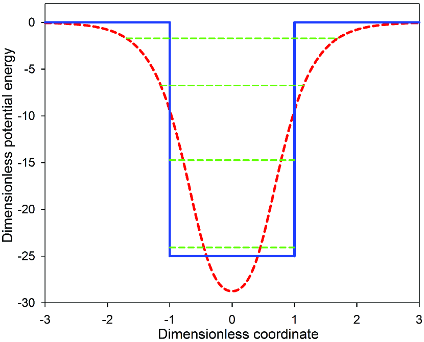
Figure 1: The isospectral reflectionless approximant (red dashed line) to a symmetric rectangular potential (blue solid line). The common energy levels are shown by green dashed lines.

Example 2: Next, let us construct a reflectionless approximant to a symmetric rectangular potential with four energy levels (see Fig. 1). These levels can be determined from (see, e.g., Schiff , Sect. II.9)

$$\kappa_{i}\,x_{i}\tan\left(\kappa_{i}\,x_{i}\right) = \sqrt{\frac{U_{0}a^{2}}{C}-\left(\kappa_{i}\,x_{i}\right)^{2}},$$ (100)

$$-\frac{\kappa_{i}\,x_{i}}{\tan\left(\kappa_{i}\,x_{i}\right)} = \sqrt{\frac{U_{0}a^{2}}{C}-\left(\kappa_{i}\,x_{i}\right)^{2}},$$ (101)

where $a$ and $U_{0}$ denote the half-width and the depth of the potential well, respectively. Eq. (100) fixes the symmetric and (101) – the antisymmetric solutions to the Schrödinger equation. Again, it is convenient to use dimensionless units for the length and energy, taking $x_{0}=a=1$ and $E_{0}=C/a^{2}=1.$ In addition, let us fix

$$\sqrt{\frac{U_{0}a^{2}}{C}}=5.$$

Then the system has four discrete levels (as assumed) corresponding to

$$\kappa_{1} = 1.3064400089,$$

$$\kappa_{2} = 2.5957390789,$$ (102)

$$\kappa_{3} = 3.8374671080,$$

$$\kappa_{4} = 4.9062951521.$$

In this case Eq. (97) cannot be further simplified, but this is not any serious problem. Indeed, let us define the coefficients $A_{i}$ and $B_{i}$, such that

$$T_{4}=\sum_{i}A_{i}\cosh(B_{i}\,x).$$

Then the corresponding potential becomes

$$V(x)=-2C\left\{\frac{\sum\limits_{i}A_{i}B_{i}^{2}\cosh(B_{i}\,x)}{\sum\limits_{i}A_{i}\cosh(B_{i}\,x)}-\left[\frac{\sum\limits_{i}A_{i}B_{i}\sinh(B_{i}\,x)}{\sum\limits_{i}A_{i}\cosh(B_{i}\,x)}\right]^{2}\right\}.$$ (103)

The result for the input data (102) can be seen in Fig. 1.

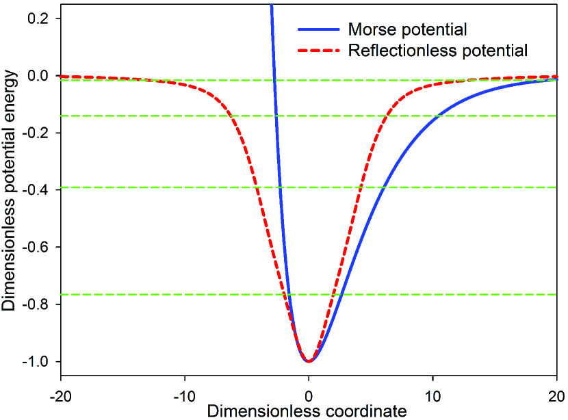
Figure 2: The isospectral reflectionless substitute to a Morse potential (see the explanations to Example 3). The common energy levels are shown by green dashed lines.

Example 3: Fig. 2 demonstrates two isospectral potentials corresponding to the following set of input parameters:

$$\kappa_{1}=1/8,\ \kappa_{2}=3/8,\ \kappa_{3}=5/8,\ \kappa_{4}=7/8,$$ (104)

the four energy levels being $E_{n}=-C\kappa_{n}^{2}$ ($n=1,2,3,4$) as previously. The solid curve in this figure corresponds to a Morse potential Morse29

$$\frac{V(x)}{D}=\exp\left(-\frac{2\alpha x}{x_{0}}\right)-2\exp\left(-\frac{\alpha x}{x_{0}}\right),$$ (105)

taking $x_{0}\equiv\sqrt{\hbar^{2}/(2mD)}=1,$ $E_{0}=D=1,$ and consequently, $C=1.$ The energy eigenvalues read

$$E_{n}=-D(1-\frac{n+1/2}{a})^{2},$$ (106)

where $a\equiv\sqrt{D/C}/\alpha.$ In Fig. 2, the value $a=4$ has been chosen, so that $\alpha=1/4$ in our dimensionless units. As in the previous example, the red dashed curve shows the symmetric reflectionless potential derived by Eq. (103) from the input parameters (104).

VI Conclusion

The main result of this work is a general formula for calculating $\tau$-functions. This important formula, Eq. (88), is a direct conclusion from Theorem 2 that has been proved with the help of well-known methods of the theory of determinants. We demonstrated that $\tau$-functions can be expanded in terms of special determinants called alternants Muir . Any alternant has a divisor – the Vandermonde’s determinant of the same order, while the quotient can be uniquely expressed as a polynomial in elementary symmetric functions (57) (see Theorem 1). Moreover, in the case of alternants related to the inverse scattering problem this quotient equals unity, i.e., the alternant itself equals the Vandermonde’s determinant. These useful properties of alternants is the key to a very simple final result expressed by Eq. (88).

Using Eqs. (88)-(89), one can uniquely reconstruct any reflectionless one-dimensional potential on the full line ($-\infty<x<\infty$), provided that the $2N$ input parameters $\kappa_{n}$ and $C_{n}$ ($n=1,2,...,N$) are known. Moreover, if the result is expected to be a symmetric function of the coordinate $x$ then the problem can be uniquely solved on the basis of the $N$ binding energies $E_{n}=-C\kappa_{n}^{2}$. Compared with the direct use of Eq. (9), the described approach significantly reduces computational efforts. Indeed, the expansions (37) and (88) contain only $2^{N-1}$ members, while Eq. (9) requires evaluation of a determinant with $N!$ members.

The efficiency of the method has been explicitly demonstrated for the case $N=4$, and there is no doubt that the algorithm can be successfully applied to a much higher number (in principle, to an arbitrary number) of given binding energies. The described approach can also be applied to building $N$-soliton solutions to the Korteweg-de Vries equation, but this would be a subject for another paper.

References

- (1) V. A. Marchenko, “Some problems of the theory of differential operators of the second order,” Dokl. Akad. Nauk SSSR 72, 457-460 (1950).
- (2) V. A. Marchenko, “Recovery of the potential energy from the scattering wave phases,” Dokl. Akad. Nauk SSSR 104, 695-698 (1955).
- (3) I. M. Gel’fand and B. M. Levitan, “Determination of a differential equation in terms of its spectral function,” Izv. Akad. Nauk SSSR. Ser. Mat. 15, 309-360 (1951) [Am. Math. Soc. Transl. (ser. 2) 1, 253 (1955)].
- (4) M. G. Krein, “On the transfer function of a one-dimensional boundary value problem of the second-order,” Dokl. Akad. Nauk SSSR 88, 405-408 (1953).
- (5) M. G. Krein, “On integral equations generating differential equations of 2nd order,” Dokl. Akad. Nauk SSSR 97, 21-24 (1954).
- (6) K. Chadan and P. C. Sabatier, Inverse Problems in Quantum Scattering Theory, 2nd ed. (Springer, New York, 1989).
- (7) I. Kay, The Inverse Scattering Problem (New York University, Institute of Mathematical Sciences, Research Report No. EM-74, 1955).
- (8) I. Kay and H. E. Moses, “The determination of the scattering potential from the spectral measure function. III,” Nuovo Cimento 3, 276-304 (1956).
- (9) L. D. Faddeev, “Relation of S-matrix and the potential for the one-dimensional Schrödinger operator,” Dokl. Akad. Nauk SSSR 121, 63-66 (1958) [Math. Rev. 20, 773 (1959)].
- (10) L. D. Faddeev, “Inverse problem of quantum scattering theory,” Usp. Mat. Nauk 14, 57-119 (1959) [J. Math. Phys. 4, 72 (1963)].
- (11) L. D. Faddeev, “Properties of the S-matrix of the one-dimensional Schrödinger equation,” Trudy Mat. Inst. Akad. Nauk SSSR 73, 314 (1964) [Amer. Math. Soc. Ser. 2 65, 139 (1967)].
- (12) L. D. Faddeev, “Inverse problem of quantum scattering theory. II,” Itogi Nauki i Tekhniki. Sovremennye Problemy Matematiki 3, 93-180 (1974) [Soviet J. Math. 5 (1976)].
- (13) V. A. Marchenko, Sturm-Liouville Operators and Applications (Naukova Dumka, Kiev, 1977) (in Russian) [Birkhäuser, Basel, 1986; revised ed.: AMS, 2011].
- (14) H. B. Thacker, C. Quigg, and J. L. Rosner, “Inverse problem for quarkonium systems. I. One-dimensional formalism and methodology,” Phys. Rev. D 18, 274-286 (1978).
- (15) C. D. Meyer, Matrix Analysis and Applied Linear Algebra (SIAM, Philadelphia, 2000).
- (16) T. Muir, A Treatise on the Theory of Determinants (Macmillan, London, 1882).
- (17) G. A. Korn and T. M. Korn, Mathematical Handbook for Scientists and Engineers (Dover, New York, 2000).
- (18) D. Cox, J. Little, and D. O’Shea, Ideals, Varieties and Algorithms, 2nd ed. (Springer, New York, 1997).
- (19) J. F. Schonfeld, W. Kwong, and J. L. Rosner, “On the convergence of reflectionless approximations to confining potentials,” Ann. Phys. 128, 1-28 (1980).
- (20) L. I. Schiff, Quantum Mechanics (McGraw-Hill, New York, 1949).
- (21) P. M. Morse, “Diatomic Molecules According to the Wave Mechanics. II. Vibrational Levels,” Phys. Rev. 34, 57-64 (1929).